VAMO: Efficient Large-Scale Nonconvex Optimization via Adaptive Zeroth Order Variance Reduction

Abstract

Optimizing large-scale nonconvex problems, common in machine learning, demands balancing rapid convergence with computational efficiency. First-order (FO) stochastic methods like SVRG provide fast convergence and good generalization but incur high costs due to full-batch gradients in large models. Conversely, zeroth-order (ZO) algorithms reduce this burden using estimated gradients, yet their slow convergence in high-dimensional settings limits practicality. We introduce VAMO (VAriance-reduced Mixed-gradient Optimizer), a stochastic variance-reduced method combining FO mini-batch gradients with lightweight ZO finite-difference probes under an SVRG-style framework. VAMO’s hybrid design uses a two-point ZO estimator to achieve a dimension-agnostic convergence rate of $\mathcal{O}(1/T+1/b)$, where $T$ is the number of iterations and $b$ is the batch-size, surpassing the dimension-dependent slowdown of purely ZO methods and significantly improving over SGD’s $\mathcal{O}(1/\sqrt{T})$ rate. Additionally, we propose a multi-point ZO variant that mitigates the $O(1/b)$ error by adjusting number of estimation points to balance convergence and cost, making it ideal for a whole range of computationally constrained scenarios. Experiments including traditional neural network training and LLM finetuning show VAMO outperforms established FO and ZO methods, offering a faster, more flexible option for improved efficiency.

1 Introduction

First-order (FO) optimization methods, particularly Stochastic Gradient Descent (SGD), have been applied in training a wide range of machine learning models. For large-scale problems, variance-reduced (VR) techniques, such as the Stochastic Variance Reduced Gradient (SVRG) algorithm allen2016improved ; reddi2016stochastic ; johnson2013accelerating , offer significant improvements, achieving faster convergence rates, $O(1/T)$, compared to the rate of SGD $O(1/\sqrt{T})$ reddi2016stochastic . However, in recent years, extremely large models—such as Large Language Models (LLMs) with billions of parameters—have become increasingly prevalent in machine learning. When training these models, traditional variance reduction methods like SVRG face a major challenge: they require periodically computing the full gradient over the entire dataset, which is often impractical for such large-scale models reddi2016stochastic . For LLMs, this step results in prohibitive computational and memory overhead, severely hindering efficient training of large models.

Zeroth-order (ZO) optimization methods present an appealing alternative in this context, as they completely bypass the need for explicit gradient calculations, estimating gradients using only function value queries nesterov2017random ; liu2018zeroth . This gradient-free characteristic drastically reduces per-iteration computational cost and memory footprint, making ZO methods attractive for resource-constrained training of LLMs malladi2023fine ; gautam2024variance . Despite these advantages, ZO methods typically exhibit slower theoretical convergence rates than FO methods and, critically, often suffer from a strong dependence on the model dimension $d$ nesterov2017random ; duchi2015optimal . Given the vast dimensionality of modern LLMs, this dependence can render pure ZO approaches impractically slow. This creates a clear dilemma for large model training: FO methods offer desirable convergence, but suffer from high gradient costs, while ZO methods are cheaper per step but often too slow and scale poorly with model size. This naturally raises the question: can we devise a hybrid strategy that combines the strengths of both FO and ZO methods, thereby overcoming their individual limitations for efficient training of large models?

In this work, we propose VAMO (VAriance-reduced Mixed-gradient Optimizer), a new adaptive hybrid algorithm specifically designed to navigate this dilemma in large-scale non-convex optimization. Our approach integrates FO and ZO techniques within the SVRG framework, aiming to maintain SVRG’s fast convergence while substantially mitigating its computational burden. A major breakthrough here is the replacement of the prohibitively expensive full FO gradient $\nabla f(\hat{\mathbf{x}})$ at SVRG checkpoints with an efficient ZO gradient estimate $\hat{\nabla}f(\hat{\mathbf{x}})$, which significantly reduces computation. This leads to a convergence rate of $O(1/T+1/b)$, significantly outperforming both ZO methods and FO-SGD, matching the rate of FO-SVRG only with an additional complexity of $O(1/b)$, which we could further decrease by increasing computational budget. The adaptability of VAMO is then enhanced through several key innovations proposed in this work. First, we introduce a novel mixing coefficient into the update rule, which enables fine-grained control over the balance between the FO stochastic gradient and the ZO variance correction term. This mechanism allows practitioners to optimize performance based on the specific characteristics of the problem and the available computational budget. Secondly, we propose a configurable ZO gradient estimation strategy for the checkpoint gradient $\hat{\nabla}f(\hat{\mathbf{x}})$, which offers a choice between the standard two-point estimator and a more robust multi-point estimator. This flexibility introduces an additional degree of control, enabling users to balance the trade-off between estimation accuracy and the number of function evaluations. Together, these innovations make VAMO highly adaptable to a wide range of optimization scenarios. Crucially, despite this hybrid and adaptive nature, our gradient estimator is designed to maintain the unbiased property inherent to FO-SVRG, distinguishing our method from many biased ZO approaches and facilitating a rigorous convergence analysis for stronger theoretical guarantees.

2 Related Work

First-order optimization. While Stochastic Gradient Descent (SGD) robbins1951stochastic remains a foundational algorithm in machine learning, its convergence can be slow in large-scale settings due to high gradient variance johnson2013accelerating . Addressing this, variance-reduced (VR) methods gower2020variance , notably SVRG allen2016improved ; reddi2016stochastic ; johnson2013accelerating and SAGA defazio2014saga , represent a significant theoretical advancement. These algorithms reduce variance by leveraging gradients from past iterates or periodically computing full-batch gradients and achieve faster convergence rates (e.g., linear convergence under certain assumptions) compared to SGD reddi2016stochastic ; johnson2013accelerating . Despite these theoretical benefits, a primary practical limitation is the substantial computational and memory cost associated with full-batch gradients. This overhead can become prohibitive as model sizes and datasets scale. Another common extension of SGD is the use of adaptive step-sizes, as in ADAM kingma2014adam and Adagrad duchi2011adaptive . However, the convergence properties of these adaptive methods remain debated and can be highly sensitive to hyper-parameter choices reddi2019convergence ; defossez2020simple ; zhang2022adam .To provide a clearer and more interpretable comparison, we focus on standard baselines such as SGD and SVRG, which better isolate the effects of our proposed modifications. Notably, our algorithm can be readily combined with adaptive step-size techniques if needed.

Zeroth-order optimization. Zeroth-order (ZO) optimization methods approximate gradients using function evaluations instead of explicit gradient computation, offering reduced computational and memory overhead zhang2024revisiting . This advantage makes them attractive for large-scale problems like large language model fine-tuning malladi2023fine ; gautam2024variance ; zhang2024revisiting ; tang2024private ; ling2024convergence , and their convergence properties are theoretically studied nesterov2017random ; liu2018zeroth ; duchi2015optimal ; jamieson2012query . However, ZO convergence rates often degrade with increasing problem dimension $d$, which makes them slow for high-dimensional models compared to FO methods liu2018zeroth ; liu2018stochastic ; wang2018stochastic . Even recent applications like MeZO malladi2023fine and MeZO-SVRG gautam2024variance are constrained by this dimensionality dependence. While ZO is crucial for black-box scenarios chen2017zoo ; tu2019autozoom , tasks like fine-tuning often have accessible gradients whose computation is merely expensive. This motivates our hybrid approach, which aims to combine ZO’s efficiency with FO’s faster convergence by strategically incorporating both types of gradient information, thereby avoiding the high computational cost associated with pure FO methods, while also mitigating the performance degradation that pure ZO methods often suffer in high-dimensional settings.

Hybrid Zeroth-Order and First-Order Algorithms. Combining the strengths of FO and ZO optimization is a relatively recent and underexplored direction, with limited established theoretical analysis. The goal is to enjoy faster convergence while using less computational resource via ZO techniques zhang2024revisiting ; li2024addax . Early explorations include schemes like applying ZO to shallower model layers and FO to deeper ones zhang2024revisiting , or concurrently computing and combining FO-SGD and ZO-SGD updates at each step, as in Addax li2024addax . However, these initial hybrid approaches may have limitations; for instance, the theoretical convergence rate of Addax still exhibits dependence on the problem dimension $d$ li2024addax , hindering its effectiveness for large-scale models. Furthermore, many early hybrid strategies often lack explicit mechanisms to adaptively tune the balance between FO accuracy and ZO query efficiency in response to varying computational resources or specific problem demands. The scarcity of hybrid strategies that offer both theoretical convergence and controlled adaptability underscores the novelty of our work.

To contextualize our contributions, Table 1 summarizes the convergence rates and computational complexities of our proposed methods, referred to as VAMO and VAMO (multi-point) in the table alongside several FO and ZO algorithms. For ZO methods, ZO-SVRG is listed with a complexity of $O(nS+bT)$ function queries. Among FO methods, FO-SGD has the lowest computational cost $O(bdT)$ but also exhibits the slowest convergence ($O(1/\sqrt{T})$). FO-SVRG improves convergence to $O(1/T)$ but increases the cost to $O(ndS+bdT)$ due to full gradient computations. Our proposed VAMO maintains a complexity of $O(nS+bdT)$, similar to ZO-SVRG in terms of $nS$ but replacing the $ndS$ full gradient cost of FO-SVRG with a cheaper $nS$ ZO estimation cost for checkpoints, while achieving a fast $O(1/T+1/b)$ convergence rate. This makes its checkpoint cost significantly slower than FO-SVRG, especially when $d$ is large. The VAMO (multi-point) variant has a complexity of $O(qnS+bdT)$. Here, increasing $q$ (the number of ZO sampling directions) leads to higher complexity for checkpoint estimation but also improves the convergence rate to $O(1/T+\frac{1}{b}(1-\frac{q}{d})^{2})$, reducing the $O(1/b)$ error term and making its performance more comparable to FO-SVRG, particularly if $q\ll d$. This demonstrates that our proposed methods provide a flexible and often more efficient trade-off between computational cost and convergence performance compared to existing pure FO or ZO approaches. Our work further develops such an adaptive hybrid approach by specifically integrating ZO estimation within the SVRG structure, aiming to reduce the full-gradient cost while preserving strong convergence guarantees independent of dimensionality.

Table 1: Summary of convergence rate and computational complexity of our proposals given $T$ total iterations. $n$ represents the total number of samples or component functions, $d$ is the problem dimension (number of parameters), $b$ denotes the mini-batch size, $S$ is the number of epochs or outer loops (for SVRG-type methods, $T\approx Sm$ where $m$ is the number of inner iterations per epoch), and $q$ signifies the number of query directions used for ZO estimation.

Method	Grad. estimator	Stepsize	Convergence rate (worst case as $b<n$)	Computational complexity
ZO-SVRG	Gradient Estimate	$O\left(\frac{1}{d}\right)$	$O\left(\frac{d}{T}+\frac{1}{b}\right)$	$O(nS+bT)$
FO-SGD	Explicit Gradient	$O\left(\frac{1}{\sqrt{T}}\right)$	$O\left(\frac{1}{\sqrt{T}}\right)$	$O(bdT)$
FO-SVRG	Explicit Gradient	$O\left(1\right)$	$O\left(\frac{1}{T}\right)$	$O(ndS+bdT)$
VAMO	Mixed Gradient	$O\left(1\right)$	$O\left(\frac{1}{T}+\frac{1}{b}\right)$	$O(nS+bdT)$
VAMO(multi-point)	Mixed Gradient	$O\left(1\right)$	$O\left(\frac{1}{T}+\frac{1}{b}(1-\frac{q}{d})^{2}\right)$	$O(qnS+bdT)$

3 Preliminaries

We consider the following nonconvex finite-sum optimization problem:

$$\min_{\mathbf{x}\in\mathbb{R}^{d}}\quad f(\mathbf{x}):=\frac{1}{n}\sum_{i=1}^{n}f_{i}(\mathbf{x}),$$ (1)

where $\{f_{i}(\mathbf{x})\}_{i=1}^{n}$ are $n$ individual nonconvex cost functions. Note that Eq. (1) is the generic form of many machine learning problems such as training neural networks, since this is the natural form arising from empirical risk minimization (ERM). Next we introduce assumptions we will make throughout the paper and provide the background of ZO gradient estimate.

3.1 Assumptions

Throughout this paper, we make the following standard assumptions on the objective function components $f_{i}(\mathbf{x})$. Let $d$ be the dimension of the optimization variable $\mathbf{x}$.

Assumption 1 (L-smooth).

Each function $f_{i}:\mathbb{R}^{d}\to\mathbb{R}$ is $L$-smooth for $i\in[n]:=\{1,2,\ldots,n\}$. That is, for any $\mathbf{x},\mathbf{y}\in\mathbb{R}^{d}$, there exists a constant $L>0$ such that:

$$\|\nabla f_{i}(\mathbf{x})-\nabla f_{i}(\mathbf{y})\|_{2}\leq L\|\mathbf{x}-\mathbf{y}\|_{2}$$

This also implies that the full objective function $f(\mathbf{x})=\frac{1}{n}\sum_{i=1}^{n}f_{i}(\mathbf{x})$ is $L$-smooth.

Assumption 2 (Bounded Variance).

The variance of the stochastic gradients is bounded. Specifically, for any $\mathbf{x}\in\mathbb{R}^{d}$, there exists a constant $\sigma^{2}\geq 0$ such that:

$$\frac{1}{n}\sum_{i=1}^{n}\|\nabla f_{i}(\mathbf{x})-\nabla f(\mathbf{x})\|_{2}^{2}\leq\sigma^{2}$$

Here, $\nabla f_{i}(\mathbf{x})$ is the gradient of a single component function, which can be viewed as a stochastic gradient of $f(\mathbf{x})$ if $i$ is chosen uniformly at random from $[n]$.

These assumptions are standard in the analysis of stochastic optimization algorithms for nonconvex problems reddi2016stochastic ; nesterov2017random ; ghadimi2013stochastic .

3.2 Convergence Notion

This work addresses the nonconvex optimization problem defined in Eq. (1), a setting prevalent in modern machine learning, particularly deep learning. In convex problems where local minima are global, …the convergence is typically measured by the expected suboptimality $\mathbb{E}\left[f(\mathbf{x}_{T})-f(\mathbf{x}^{*})\right]$. However, in nonconvex settings, identifying a global minimum is generally intractable due to the potential presence of multiple local minima and saddle points dauphin2014identifying ; balasubramanian2022zeroth .

Consequently, for such nonconvex problems, the convergence is evaluated by the first-order stationary condition in terms of the expected squared gradient norm $\mathbb{E}[\|\nabla f(\mathbf{x})\|_{2}^{2}]$. An algorithm is considered to converge if this metric approaches zero or falls below a specified tolerance $\epsilon$ liu2020primer ; mu2024variance . It serves as the primary metric for the theoretical convergence guarantees presented in this paper.

3.3 ZO Gradient Estimation

Consider an individual cost function $f_{i}:\mathbb{R}^{d}\to\mathbb{R}$ that satisfies the conditions in Assumption 1. The ZO approach estimates gradients using only function evaluations.

A commonly used two-point ZO gradient estimator for $f_{i}(\mathbf{x})$ is defined as nesterov2017random ; spall1992multivariate :

$$\hat{\nabla}f_{i}(\mathbf{x})=\frac{d}{\mu}\left[f_{i}(\mathbf{x}+\mu\mathbf{u}_{i})-f_{i}(\mathbf{x})\right]\mathbf{u}_{i},\quad\text{for }i\in[n],$$ (2)

where $d$ is the dimensionality of the parameter vector $\mathbf{x}$, $\mu>0$ is a small smoothing parameter, and $\{\mathbf{u}_{i}\}_{i=1}^{n}$ are i.i.d. random direction vectors drawn uniformly from the unit Euclidean sphere in $\mathbb{R}^{d}$ (i.e., $\mathbf{u}_{i}\sim U(\mathbb{S}^{d-1})$) flaxman2004online ; shamir2017optimal ; gao2018information .

In general, for $\mu>0$, the ZO gradient estimator $\hat{\nabla}f_{i}(\mathbf{x})$ is a biased approximation of the true gradient $\nabla f_{i}(\mathbf{x})$. The bias tends to decrease as $\mu\to 0$. However, in practical implementations, choosing an excessively small $\mu$ can render the function difference $f_{i}(\mathbf{x}+\mu\mathbf{u}_{i})-f_{i}(\mathbf{x})$ highly sensitive to numerical errors or system noise or numerical precision issues, potentially failing to accurately represent the local change in the function lian2016comprehensive . A key property of the ZO estimator is that for $\mu>0$, it provides an unbiased estimate of the gradient of a smoothed version of $f_{i}$, often denoted $f_{i,\mu}(\mathbf{x})=\mathbb{E}_{\mathbf{v}}[f_{i}(\mathbf{x}+\mu\mathbf{v})]$ (where $\mathbf{v}$ is a random vector from a unit ball or sphere), i.e., $\mathbb{E}_{\mathbf{u}_{i}}[\hat{\nabla}f_{i}(\mathbf{x})]=\nabla f_{i,\mu}(\mathbf{x})$ liu2020primer .

To reduce the variance of the ZO gradient estimate, a multi-point version can be employed. Instead of using a single random direction $\mathbf{u}_{i}$, $q\geq 1$ i.i.d. random directions $\{\mathbf{u}_{i,j}\}_{j=1}^{q}$ are sampled for each $f_{i}$. Since estimating along each direction requires two function queries, the multi-point ZO gradient estimator involves a total of $2q$ function queries and is defined as duchi2015optimal ; liu2020primer :

$$\hat{\nabla}f_{i}(\mathbf{x})=\frac{d}{\mu q}\sum_{j=1}^{q}\left[f_{i}(\mathbf{x}+\mu\mathbf{u}_{i,j})-f_{i}(\mathbf{x})\right]\mathbf{u}_{i,j},\quad\text{for }i\in[n].$$ (3)

We refer to this as the multi-point ZO gradient estimate throughout the paper.

3.4 Notations

In this paper, we denote $\nabla f(x),\nabla f_{i}(x)$ as first-order gradients of $f(x)$ and $f_{i}(x)$, respectively. Also denote $\hat{\nabla}f(x),\hat{\nabla}f_{i}(x)$ as their zeroth-order variants. $\mathbb{E}[\cdot]$ operates as the usual mathematical expectation, and $\mathcal{I}$ is a mini-batch of indices sampled from $[n]:={1,\dots,n}$, with size $b=|\mathcal{I}|$. $\|\cdot\|_{2}$ denotes the Euclidean/l2 norm as per usual.

4 Hybrid FO and ZO Stochastic Variance Reduction (VAMO)

4.1 From SVRG and ZO-SVRG to Hybrid SVRG

The principles of FO-SVRG and ZO-SVRG have been extensively explored in optimization literature reddi2016stochastic ; johnson2013accelerating ; liu2018zeroth ; ji2019improved . FO-SVRG, in particular, is known to achieve a linear convergence rate $O(1/T)$ for non-convex problems under certain conditions, significantly outperforming the convergence rate of FO-SGD reddi2016stochastic . The key step of FO-SVRG involves leveraging a full gradient $\nabla f(\hat{\mathbf{x}})$, computed periodically at a checkpoint $\hat{\mathbf{x}}$, to construct a variance-reduced stochastic gradient estimate johnson2013accelerating :

$$\hat{\mathbf{g}}_{\text{FO-SVRG}}=\nabla f_{\mathcal{I}}(\mathbf{x})-\nabla f_{\mathcal{I}}(\hat{\mathbf{x}})+\nabla f(\hat{\mathbf{x}}),$$ (4)

where $\nabla f_{\mathcal{I}}(\mathbf{x})=\frac{1}{b}\sum_{i\in\mathcal{I}}\nabla f_{i}(\mathbf{x})$ is the mini-batch stochastic gradient from a subset $\mathcal{I}\subseteq[n]$ of size $b$. A crucial property of $\hat{\mathbf{g}}_{\text{FO-SVRG}}$ is that $\hat{\mathbf{g}}_{\text{FO-SVRG}}$ is an unbiased gradient estimate of $\nabla f(\mathbf{x})$, $\mathbb{E}[\hat{\mathbf{g}}_{\text{FO-SVRG}}]=\nabla f(\mathbf{x})$.

In the ZO setting, ZO-SVRG adapts the SVRG structure by replacing all explicit gradient computations with ZO estimates derived from function evaluations:

$$\hat{\mathbf{g}}_{\text{ZO-SVRG}}=\hat{\nabla}f_{\mathcal{I}}(\mathbf{x})-\hat{\nabla}f_{\mathcal{I}_{k}}(\hat{\mathbf{x}})+\hat{\nabla}f(\hat{\mathbf{x}}),$$ (5)

where $\hat{\nabla}f_{\mathcal{I}}(\mathbf{x})=(1/b)\sum_{i\in\mathcal{I}}\hat{\nabla}f_{i}(\mathbf{x})$, $\hat{\nabla}f(\mathbf{x})=\hat{\nabla}f_{[n]}(\mathbf{x})$, and $\hat{\nabla}f_{i}(\mathbf{x})$ is a ZO gradient estimate (e.g., two-point or multi-point as defined in Section 3.3). While structurally similar, a key distinction is that $\hat{\mathbf{g}}_{\text{ZO-SVRG}}$ is generally a biased estimate of $\nabla f(\mathbf{x})$ due to the inherent bias of $\hat{\nabla}f_{i}(\mathbf{x})$ relative to $\nabla f_{i}(\mathbf{x})$. This bias significantly complicates its convergence analysis compared to FO-SVRG.

VAMO (Algorithm 1) is motivated by the high cost of computing the full gradient $\nabla f(\hat{\mathbf{x}})$ in SVRG for large-scale models, and introduces a hybrid gradient estimator that combines FO and ZO components to reduce this overhead:

$$\hat{\mathbf{g}}=\nabla f_{\mathcal{I}}(\mathbf{x})-\alpha\left(\hat{\nabla}f_{\mathcal{I}}(\hat{\mathbf{x}})-\hat{\nabla}f(\hat{\mathbf{x}})\right).$$ (6)

Here, $\nabla f_{\mathcal{I}}(\mathbf{x})$ is the standard FO mini-batch stochastic gradient at the current iterate $\mathbf{x}$, while $\hat{\nabla}f(\hat{\mathbf{x}})$ is the ZO estimate of the full gradient at the checkpoint $\hat{\mathbf{x}}$.

A critical design choice in Eq. (6) is the construction of the variance-reduction term $\alpha\left(\hat{\nabla}f_{\mathcal{I}}(\hat{\mathbf{x}})-\hat{\nabla}f(\hat{\mathbf{x}})\right)$. To preserve the desirable unbiased property of SVRG, we ensure that the expectation of the ZO-based correction term, $\mathbb{E}\left[\hat{\nabla}f_{\mathcal{I}}(\hat{\mathbf{x}})-\hat{\nabla}f(\hat{\mathbf{x}})\right]$, is zero. Using ZO estimates for both terms within the parentheses, $\hat{\nabla}f_{\mathcal{I}}(\hat{\mathbf{x}})$ and $\hat{\nabla}f(\hat{\mathbf{x}})$, rather than mixing FO and ZO estimates within that difference, is key to this property and also contributes to computational savings at the checkpoint. Maintaining this unbiasedness is pivotal, as it allows for a more tractable convergence analysis akin to FO-SVRG, distinguishing our approach from many ZO algorithms that contend with biased estimators.

Furthermore, VAMO introduces a novel mixing coefficient $\alpha>0$. This parameter, absent in traditional SVRG or ZO-SVRG, allows for explicit control over the influence of the ZO-derived variance term. The choice of $\alpha$, which we will discuss in Section 5.1, enables a flexible balance between computational overhead and convergence performance.

The introduction of this hybrid structure, particularly the ZO estimation at checkpoints and the mixing coefficient $\alpha$, means that the convergence analysis of VAMO cannot be trivially inherited from existing FO-SVRG or ZO-SVRG analyses. It requires a dedicated theoretical investigation to characterize its behavior and prove its convergence guarantees, which constitutes a core part of our contribution in Section 4.2. This distinct analytical challenge underscores the theoretical novelty of our work.

Algorithm 1 VAMO$(T,m,\{\eta_{k}\},b,\bar{x}_{0},\mu,\alpha)$

1: Input: In addition to parameters in SVRG, set smoothing parameter $\mu>0$.

2: for $s=1,2,\dots,S$ do

3:  compute ZO estimate $\hat{g}_{s}=\hat{\nabla}f(\bar{x}_{s-1})$

4:  set $x_{0}^{s}=\bar{x}_{s-1}$

5:  for $k=0,1,\dots,m-1$ do

6:   choose mini-batch $I_{k}$ of size $b$

7:   compute hybrid FO and ZO gradient blending (6): $\mathbf{v}_{k}^{s}=\nabla f_{I_{k}}(x_{k}^{s})-\alpha(\hat{\nabla}f_{I_{k}}(x_{0}^{s})-\hat{g}_{s})$

8:   update $x_{k+1}^{s}=x_{k}^{s}-\eta_{k}\mathbf{v}_{k}^{s}$

9:  end for

10:  set $\bar{x}_{s}=x_{m}^{s}$

11: end for

12: return $\bar{x}$ chosen uniformly at random from $\{\{x_{k}^{s}\}^{m-1}_{k=0}\}^{S}_{s=1}$.

4.2 Convergence analysis

In this section, we present the convergence analysis for VAMO using the two-point ZO gradient estimate (Eq. (2)). Our analysis is based on an upper bound on the expected squared gradient norm $\mathbb{E}\bigl{[}\|\nabla f(\bar{\mathbf{x}})\|_{2}^{2}\bigr{]}$, as shown in Theorem 1. As discussed in Section 3.2, for non-convex objectives, a small value of $\mathbb{E}\bigl{[}\|\nabla f(\bar{\mathbf{x}})\|_{2}^{2}\bigr{]}$ implies convergence to a stationary point.

Theorem 1.

Under the assumptions in Section 3.1, and the two-point ZO gradient estimate is used. The output $\bar{\mathbf{x}}$ of Algorithm 1 satisfies:

$$\mathbb{E}\bigl{[}\|\nabla f(\bar{\mathbf{x}})\|_{2}^{2}\bigr{]} \leq\frac{\mathbb{E}[f(\bar{\mathbf{x}}_{0})-f^{*}]}{T\bar{\gamma}}+\frac{S\chi_{m}}{T\bar{\gamma}},$$ (7)

where $T=Sm$, $f^{*}=\min_{\mathbf{x}}f(\mathbf{x})$, $\bar{\gamma}=\min_{k\in[m]}\gamma_{k}$, and $\chi_{m}=\sum_{k=0}^{m-1}\chi_{k}$ with

$$\gamma_{k} =\biggl{(}1-\frac{c_{k+1}}{\beta_{k}}\biggr{)}\eta_{k}-4\biggl{(}\frac{L}{2}+c_{k+1}\biggr{)}\times\biggl{(}2\alpha^{2}-2\alpha+1+\frac{24d\delta_{n}}{b}\alpha^{2}\biggr{)}\eta_{k}^{2},$$ (8)

$$\chi_{k} =\biggl{(}\frac{L}{2}+c_{k+1}\biggr{)}\times\biggl{(}\frac{9\delta_{n}}{b}d^{2}L^{2}\mu^{2}\alpha^{2}+\frac{4\sigma^{2}}{b}\bigl{(}4d\delta_{n}\alpha^{2}+(1-\alpha)^{2}\bigr{)}\biggr{)}\eta_{k}^{2}.$$ (9)

The coefficients $\{c_{k}\}$ are given by:

$$c_{k}=\biggl{[}1+\beta_{k}\eta_{k}+\frac{6(4d+1)L^{2}\delta_{n}\eta_{k}^{2}}{b}\biggr{]}c_{k+1}+\frac{3(4d+1)L^{3}\delta_{n}\eta_{k}^{2}}{b},\quad c_{m}=0.$$ (10)

Proof. See Appendix A.3.

Compared to the convergence rate of SVRG reddi2016stochastic , Theorem 1 has an additional error $\left(\frac{S\chi_{m}}{T\bar{\gamma}}\right)$ because of the use of ZO gradient estimator. $\chi_{m}$ depends on the epoch $m$, the step size $\eta_{k}$, the smoothing parameter $\mu$, the mini-batch size $b$, the number of optimization variables $d$ and the mixing constant $\alpha$. To obtain a clear dependence on these parameters and explore deeper convergence insights, we simplify (7) to suit specific parameter settings, as shown below.

Corollary 1.

Suppose parameters are set as

$$\mu=\frac{1}{\sqrt{T}},\quad\eta_{k}=\eta=\frac{\rho}{L},\quad\alpha=\frac{1}{d},$$ (11)

with $\beta_{k}=\beta=L$, where $0<\rho\leq 1$ is a universal constant independent of $b$, $d$, $\alpha$, $L$ and $T$. Then Theorem 1 implies

$$\frac{\mathbb{E}[f(\bar{\mathbf{x}}_{0})-f^{*}]}{T\bar{\gamma}}\leq O\biggl{(}\frac{1}{T}\biggr{)},\quad\frac{S\chi_{m}}{T\bar{\gamma}}\leq O\biggl{(}\frac{1}{bT}+\frac{1}{b}\biggr{)},$$ (12)

yielding the convergence rate:

$$\mathbb{E}\bigl{[}\|\nabla f(\bar{\mathbf{x}})\|_{2}^{2}\bigr{]}\leq O\biggl{(}\frac{1}{T}+\frac{1}{bT}+\frac{1}{b}\biggr{)}.$$ (13)

Proof. See Appendix A.4.

From Corollary 1, we can observe that one advantage of this algorithm is that, compared to previous ZO algorithms, the value of smoothing parameters $\mu$ is less restrictive. For example, ZO-SVRG liu2018zeroth required $\mu\leq O(d^{-1/2}T^{-1/2})$, and ZO-SGD ghadimi2013stochastic required $\mu\leq O(d^{-1}T^{-1/2})$. Compared to FO-SGD, the algorithm achieves an improved rate of $O(1/T)$ rather than the rate of $O(1/\sqrt{T})$. Compared to ZO algorithms, the convergence rate is independent of the number of optimization variables $d$. Compared to first-order SVRG. though both methods achieve a linear convergence rate, VAMO suffers an additional error of $O(1/b)$ inherited from $\frac{S\chi_{m}}{T\bar{\gamma}}$ in (1).

5 VAMO with Multi-Point ZO Gradient Estimation

Building upon the VAMO algorithm previously introduced with a two-point ZO gradient estimator, this section presents its multi-point ZO estimation variant. This extension is a key component of VAMO’s adaptive design, as adjusting the number of random directions $q$ in ZO estimate allows for explicit tuning of the trade-off between computational cost and the precision of the ZO-based variance reduction, thereby directly influencing convergence performance.

Theorem 2.

Suppose assumptions A1 and A2 hold, and the multi-point ZO gradient estimate is used in Algorithm 1. The gradient norm bound in (7) yields the simplified convergence rate:

$$\mathbb{E}\bigl{[}\|\nabla f(\bar{\mathbf{x}})\|_{2}^{2}\bigr{]}\leq O\biggl{(}\frac{1}{T}+\frac{1}{bT}+\frac{1}{b}\Bigl{(}1-\frac{q}{d}\Bigr{)}^{2}\biggr{)}.$$ (14)

With parameter choices $\mu=\frac{1}{q\sqrt{T}}$, $\eta=\frac{\rho}{L}$, $\alpha=\frac{q}{d}$, and $\beta=L$, the coefficients satisfy:

$$c_{k} =\biggl{(}1+\beta_{k}\eta_{k}\biggr{)}c_{k+1}+\biggl{(}\frac{L}{2}+c_{k+1}\biggr{)}\biggl{(}1+\frac{4d}{q}\biggr{)}\frac{12L^{2}\delta_{n}\eta_{k}^{2}\alpha^{2}}{b},$$ (15)

$$\gamma_{k} =\eta_{k}-\frac{c_{k+1}\eta_{k}}{\beta_{k}}-4\biggl{(}\frac{L}{2}\eta_{k}^{2}+c_{k+1}\eta_{k}^{2}\biggr{)}\biggl{(}\Bigl{(}2+\frac{24d\delta_{n}}{qb}\Bigr{)}\alpha^{2}-2\alpha+1\biggr{)},$$ (16)

$$\chi_{k} =\biggl{(}\frac{L}{2}\eta_{k}^{2}+c_{k+1}\eta_{k}^{2}\biggr{)}\times\biggl{(}\frac{3\delta_{n}}{b}\Bigl{(}1+\frac{2}{q}\Bigr{)}L^{2}d^{2}\mu^{2}\alpha^{2}+\frac{4\sigma^{2}}{b}\Bigl{(}\frac{24d\delta_{n}\alpha^{2}}{q}+(1-\alpha)^{2}\Bigr{)}\biggr{)}.$$ (17)

Proof. See Appendix A.5.

By contrast with Corollary 1, it can be seen from Eq. (14) that the use of multi-point version of VAMO reduces the error $O(1/b)$ in Eq. (1) by leveraging multiple $q$ direction sampling, while increasing the computational cost accordingly. If $q=d$, the algorithm’s computational cost and convergence rate become comparable to FO-SVRG. Please note that the smoothing parameter $\mu$ is more restrictive than that in two-point version of VAMO for reducing the error. A comprehensive summary and comparison of the computational complexities and convergence rates of our proposed VAMO methods against various FO and ZO algorithms can be found in Table 1, which is presented and discussed in Section 2.

5.1 Balancing FO and ZO Information via $\alpha$

The mixing coefficient $\alpha$ in the VAMO update (Eq. (6)) critically balances the FO stochastic gradient $\nabla f_{\mathcal{I}}(\mathbf{x})$ against the ZO variance correction term $\hat{\nabla}f_{\mathcal{I}}(\hat{\mathbf{x}})-\hat{\nabla}f(\hat{\mathbf{x}})$. The optimal choice for $\alpha$ directly depends on the estimation error $\omega_{i}$ inherent in the ZO gradient components ($\hat{\nabla}f_{i}(\mathbf{x})=\nabla f_{i}(\mathbf{x})+\omega_{i}$). As established in the literature liu2018zeroth ; liu2020primer and detailed in Appendix A.7, the expected squared ZO error $\mathbb{E}[|\omega_{i}|_{2}^{2}]$ typically scales as $\mathcal{O}(d)$ for two-point estimates and $\mathcal{O}(d/q)$ for multi-point estimates using $q$ random directions. fThis relationship dictates that $\alpha$ should reflect the trustworthiness of the ZO estimates: when the ZO error is substantial (e.g., large $d$, small $q$), a smaller $\alpha$ is warranted to prevent amplifying this error. Conversely, when ZO estimates are more reliable (e.g., larger $q$ reducing error), a larger $\alpha$ can more aggressively leverage the variance reduction. This principled inverse relationship between ZO error magnitude (influenced by $d$ and $q$) and the appropriate scale of $\alpha$ is key. While specific forms like $\alpha\propto 1/d$ or $\alpha\propto q/d$ analyzed in our theoretical sections (e.g., Corollary 1 and Theorem 2) illustrate this adaptive trend, the core insight is that $\alpha$ must be adjusted to counterbalance the ZO estimator’s error profile. Such adaptability enables VAMO to effectively navigate the trade-off between computational cost and convergence performance, a central aspect of its practical utility.

6 Applications and Experiments

In this section, we present empirical results to validate the effectiveness and adaptability of the proposed VAMO. We first demonstrate VAMO’s adaptive capabilities by evaluating the impact of its key tunable component, the number of ZO random directions ($q$), on a synthetic task, showcasing how performance can be configured based on computational budget. Subsequently, we benchmark its performance against standard FO and ZO methods on a classification task using DNNs, and finally, we demonstrate its utility in a large model fine-tuning scenario gautam2024variance . Detailed experimental setups and hyperparameter settings for all methods and tasks are provided in Appendix A.8,  A.9 and  A.10.

Adaptability Experiment: Nonconvex Least Squares with Varying $q$ To showcase VAMO’s adaptive nature and empirically validate the theoretical benefits of its multi-point ZO estimation strategy (as discussed in Section 5), we conducted experiments on a synthetic non-convex least-squares task. The objective was $f(\mathbf{x})=\frac{1}{n}\sum_{i=1}^{n}(h(\mathbf{x};\mathbf{z}_{i})-y_{i})^{2}$, with $n=1000$ component functions and a parameter dimension $d=100$, where $h(\mathbf{x};\cdot)$ was parameterized by a simple non-convex neural network. We compared VAMO variants using $q\in\{1,3,5\}$ (number of ZO query directions for the multi-point ZO gradient estimator) against the classical FO-SGD algorithm.

Fig. 1(a) presents the training loss convergence. Consistent with our theoretical analysis (see Table 1), all VAMO variants achieve an $O(1/T)$ convergence rate, outperforming FO-SGD’s $O(1/\sqrt{T})$ rate. The figure clearly illustrates VAMO’s adaptability: increasing $q$ improves convergence performance, effectively mitigating the additional $O(1/b)$ error term associated with the two-point ($q=1$) variant. This aligns with the theoretical prediction that this error term diminishes for larger $q$ (scaling towards $O(\frac{1}{b}(1-q/d)^{2})$). These results empirically validate our theory and highlight VAMO’s practical ability to adaptively trade computational cost (via varying $q$) for enhanced convergence by managing ZO estimation error, a key aspect of its flexible and adaptive design.

Multiclass Classification For this benchmark on the MNIST dataset lecun1998gradient , we trained a Multi-Layer Perceptron (MLP) and compared our proposed VAMO (two-point version, $q=1$) against FO-SGD robbins1951stochastic , ZO-SGD ghadimi2013stochastic , and ZO-SVRG liu2018zeroth . As illustrated by the training loss convergence in Fig. 1(b), our VAMO algorithm demonstrates a significant performance advantage over the purely ZO methods (ZO-SGD and ZO-SVRG), achieving both substantially faster convergence and a better final loss value. Moreover, VAMO’s convergence behavior is highly competitive with that of the standard FO-SGD algorithm. These findings underscore the practical effectiveness of our hybrid strategy.

GPT2 Fine-Tuning To further assess VAMO’s practical utility and its advantages in complex, large-scale settings, we applied it to the task of fine-tuning a pre-trained GPT-2 model radford2019language . Specifically, this experiment involved fine-tuning the base GPT-2 model on the MultiNLI (MNLI) dataset williams2017broad for a natural language inference task. Our proposed VAMO algorithm was benchmarked against key FO optimizers, notably FO-SGD robbins1951stochastic , and representative ZO methods such as ZO-SGD and ZO-SVRG.

In Fig. 2, we present training loss against iteration steps and queries, highlighting VAMO’s practical advantages, with the query-based evaluation in Fig. 2(b) focusing on its comparison with FO-SGD. To clearly distinguish from potential ZO query definitions and to establish a consistent basis for comparison with FO methods, a query here is specifically defined in terms of FO computational units: it denotes a single pass (either forward or backward) of one data sample through the model; consequently, an FO mini-batch gradient calculation on $b$ samples costs $2b$ queries. According to Table 1, VAMO incurs an additional query cost over FO-SGD due to the use of the full ZO gradient. FO-SGD has a total computational cost of $O(bdT)$, while VAMO incurs an additional $O(nS)$ cost. For large models such as GPT-2 (e.g., $d\approx 1.2\times 10^{8},n\approx 256,m=10,b=32$, with $T=Sm$), this leads to only a minor fractional overhead of approximately $n/(2bdm)$ compared to FO-SGD, assuming the per-step ZO correction is also query-light. Therefore, with a total query cost only slightly higher than that of FO-SGD, VAMO achieves significantly faster and more stable convergence per query, as demonstrated in Fig. 2(b). This improvement stems from its variance-reduced SVRG backbone, now made efficient and practical through ZO techniques.

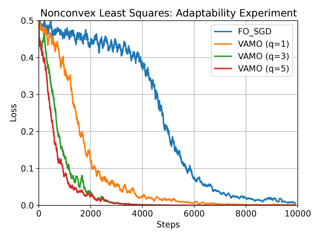
(a)

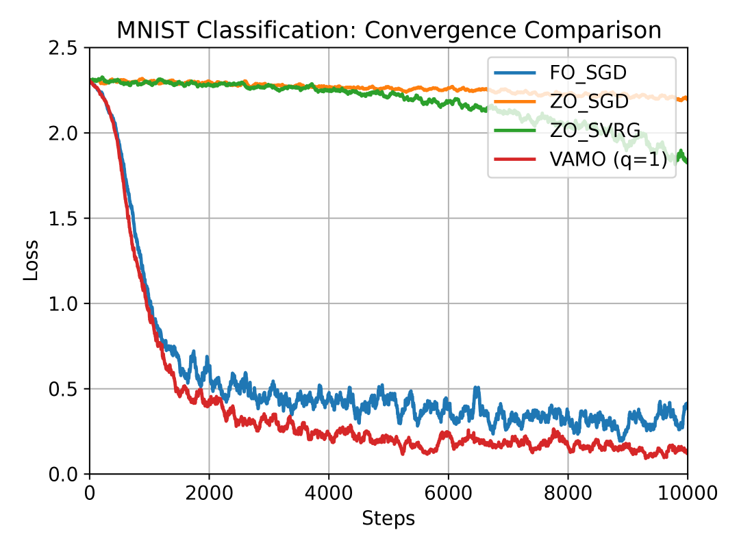
(b)

Figure 1: (a) Convergence comparison on a non-convex least-squares task, showing VAMO with varying ZO query points ($q=1,3,5$) against FO-SGD. (b) Convergence comparison on the MNIST classification task against pure FO and ZO methods.

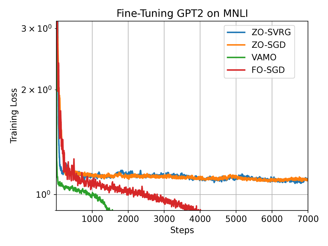
(a) Training loss versus iteration steps

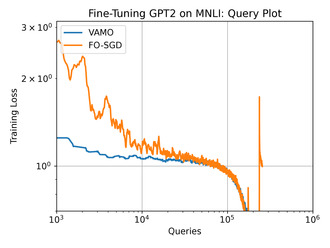
(b) Training loss versus queries

Figure 2: Convergence comparison on the fine-tuning GPT2 task against pure FO and ZO methods.

7 Conclusion

In this paper, we propose a hybrid FO and ZO variance-reduced algorithm, VAMO, for nonconvex optimization. We demonstrate that compared to FO-SGD, our algorithm improves the convergence rate from $O(1/\sqrt{T})$ to a linear rate of $O(1/T)$, achieving convergence performance similar to FO-SVRG. Compared to ZO algorithms, our method maintains convergence performance independent of the problem dimension $d$, making it effective for optimizing high-dimensional problems. However, due to the use of two-point ZO gradient estimation, our convergence result includes an additional error term $O(1/b)$. To mitigate this, we introduce a multi-point ZO gradient estimation variant, which reduces this error. Unlike previous purely FO or ZO methods, our hybrid approach leverages the advantages of both, enabling a more flexible trade-off between computational efficiency and convergence performance. This makes it more adaptable to real-world applications with complex constraints. Our theoretical analysis and empirical evaluations, including comparisons with state-of-the-art methods, demonstrate the effectiveness of our approach.

Appendix A Appendix / supplemental material

A.1 ZO gradient estimator

Lemma 1.

Under the assumptions in Section 3.1, and define $f_{\mu}=\mathbb{E}_{\mathbf{u}\sim U_{b}}[f(\mathbf{x}+\mu\mathbf{u})]$ where $U_{b}$ is the uniform distribution over the unit Euclidean ball. Then:

1. $f_{\mu}$ is $L$-smooth with

   $$\nabla f_{\mu}(\mathbf{x})=\mathbb{E}_{\mathbf{u}}\bigl{[}\hat{\nabla}f(\mathbf{x})\bigr{]}.$$ (18)

2. For any $\mathbf{x}\in\mathbb{R}^{d}$:

   $$|f_{\mu}(\mathbf{x})-f(\mathbf{x})|\leq\frac{L\mu^{2}}{2},$$ (19)

   $$\|\nabla f_{\mu}(\mathbf{x})-\nabla f(\mathbf{x})\|_{2}^{2}\leq\frac{\mu^{2}L^{2}d^{2}}{4},$$ (20)

   $$\frac{1}{2}\|\nabla f(\mathbf{x})\|_{2}^{2}-\frac{\mu^{2}L^{2}d^{2}}{4}\leq\|\nabla f_{\mu}(\mathbf{x})\|_{2}^{2}\leq 2\|\nabla f(\mathbf{x})\|_{2}^{2}+\frac{\mu^{2}L^{2}d^{2}}{2}.$$ (21)

3. For any $\mathbf{x}\in\mathbb{R}^{d}$:

   $$\mathbb{E}_{\mathbf{u}}\bigl{[}\|\hat{\nabla}f(\mathbf{x})-\nabla f_{\mu}(\mathbf{x})\|_{2}^{2}\bigr{]}\leq 2d\|\nabla f(\mathbf{x})\|_{2}^{2}+\frac{\mu^{2}L^{2}d^{2}}{2}.$$ (22)

Proof.

See the proof of Lemma 1 in liu2018zeroth ∎

Lemma 2.

Under the conditions of Lemma 1:

1. For any $\mathbf{x}\in\mathbb{R}^{d}$:

   $$\nabla f_{\mu}(\mathbf{x})=\mathbb{E}_{\mathbf{u}}\bigl{[}\hat{\nabla}f(\mathbf{x})\bigr{]}.$$ (23)

   where $\hat{\nabla}f(\mathbf{x})$ is the multi-point gradient estimate.

2. For any $\mathbf{x}\in\mathbb{R}^{d}$:

   $$\mathbb{E}\bigl{[}\|\hat{\nabla}f(\mathbf{x})-\nabla f_{\mu}(\mathbf{x})\|_{2}^{2}\bigr{]}\leq\frac{2d}{q}\|\nabla f(\mathbf{x})\|_{2}^{2}+\frac{\mu^{2}L^{2}d^{2}}{2q}.$$ (24)

Proof.

See the proof of Lemma 2 in liu2018zeroth ∎

A.2 Second-Order Moment of the Hybrid Gradient Estimator

The primary goal of our convergence analysis is to establish theoretical guarantees for VAMO in solving non-convex optimization problems. Specifically, we aim to bound the expected squared norm of the gradient, $\mathbb{E}[\|\nabla f(\bar{\mathbf{x}})\|_{2}^{2}]$, as shown in Theorem 1. Due to the hybrid structure of the gradient estimator $\mathbf{v}_{k}^{s}$ used in VAMO, directly analyzing the final convergence metric is challenging. As a key intermediate step, we first derive an upper bound on the second-order moment $\mathbb{E}[\|\mathbf{v}_{k}^{s}\|_{2}^{2}]$.

Proposition 1.

Under the assumptions in Section 3.1, and two-point ZO gradient estimate is used in Algorithm 1. The blended gradient $\mathbf{v}_{k}^{s}$ in Step 7 of Algorithm 1 satisfies,

$$\begin{split}\mathbb{E}\bigl{[}\|{\mathbf{v}}_{k}^{s}\|_{2}^{2}\bigr{]}&\leq 4\biggl{(}2\alpha^{2}-2\alpha+1+\frac{24d\delta_{n}}{b}\alpha^{2}\biggr{)}\mathbb{E}\bigl{[}\|\nabla f(\mathbf{x}_{k}^{s})\|_{2}^{2}\bigr{]}\\ &\quad+\frac{12\delta_{n}(4d+1)L^{2}}{b}\alpha^{2}\mathbb{E}\bigl{[}\|\mathbf{x}_{0}^{s}-\mathbf{x}_{k}^{s}\|_{2}^{2}\bigr{]}\\ &\quad+\frac{9\delta_{n}}{b}d^{2}L^{2}\mu^{2}\alpha^{2}+\frac{4\sigma^{2}}{b}\biggl{(}24d\delta_{n}\alpha^{2}+(1-\alpha)^{2}\biggr{)},\end{split}$$ (25)

where $\delta_{n}=1$ if the mini-batch contains $i.i.d$. samples from $[n]$ with replacement, and $\delta_{n}=I(b<n)$ if samples are randomly selected without replacement. Here $I(b<n)$ is 1 if $b<n$, and 0 if $b=n$.

Proof.

In Algorithm 1, we recall that the mini-batch $\mathcal{I}$ is chosen uniformly randomly (with replacement). It is known from Lemma 1 and Lemma 3 that

$$\mathbb{E}_{\mathcal{I}_{k}}\left[\nabla{f}_{\mathcal{I}_{k}}(\mathbf{x}_{k}^{s})-\hat{\nabla}{f}_{\mathcal{I}_{k}}(\mathbf{x}_{0}^{s})\right]=\nabla f(\mathbf{x}_{k}^{s})-\hat{\nabla}f(\mathbf{x}_{0}^{s}).$$ (26)

We then rewrite $\mathbf{v}_{k}^{s}$ as

$$\mathbf{v}_{k}^{s} =\left(1-\alpha\right)\nabla{f}_{\mathcal{I}_{k}}(\mathbf{x}_{k}^{s})$$ (27)

$$+\alpha\left(\nabla{f}_{\mathcal{I}_{k}}(\mathbf{x}_{k}^{s})-\hat{\nabla}{f}_{\mathcal{I}_{k}}(\mathbf{x}_{0}^{s})-\mathbb{E}_{\mathcal{I}_{k}}\left[\nabla{f}_{\mathcal{I}_{k}}(\mathbf{x}_{k}^{s})-\hat{\nabla}{f}_{\mathcal{I}_{k}}(\mathbf{x}_{0}^{s})\right]+\nabla f(\mathbf{x}_{k}^{s})\right)$$

Taking the expectation of $\left\|\mathbf{v}_{k}^{s}\right\|_{2}^{2}$ with respect to all the random variables, we have

$$\mathbb{E}\left[\left\|\mathbf{v}_{k}^{s}\right\|_{2}^{2}\right] \leq 2\left(1-\alpha\right)^{2}\mathbb{E}\left[\left\|\nabla{f}_{\mathcal{I}_{k}}(\mathbf{x}_{k}^{s})\right\|_{2}^{2}\right]$$ (28)

$$+2\alpha^{2}\mathbb{E}\left[\left\|\nabla{f}_{\mathcal{I}_{k}}(\mathbf{x}_{k}^{s})-\hat{\nabla}{f}_{\mathcal{I}_{k}}(\mathbf{x}_{0}^{s})-\mathbb{E}_{\mathcal{I}_{k}}\left[\nabla{f}_{\mathcal{I}_{k}}(\mathbf{x}_{k}^{s})-\hat{\nabla}{f}_{\mathcal{I}_{k}}(\mathbf{x}_{0}^{s})\right]+\nabla f(\mathbf{x}_{k}^{s})\right\|_{2}^{2}\right]$$

$$\leq 4\alpha^{2}\mathbb{E}\left[\left\|\nabla{f}_{\mathcal{I}_{k}}(\mathbf{x}_{k}^{s})-\hat{\nabla}{f}_{\mathcal{I}_{k}}(\mathbf{x}_{0}^{s})-\mathbb{E}_{\mathcal{I}_{k}}\left[\nabla{f}_{\mathcal{I}_{k}}(\mathbf{x}_{k}^{s})-\hat{\nabla}{f}_{\mathcal{I}_{k}}(\mathbf{x}_{0}^{s})\right]\right\|_{2}^{2}\right]$$

$$+4\alpha^{2}\mathbb{E}\left[\left\|\nabla f(\mathbf{x}_{k}^{s})\right\|_{2}^{2}\right]+2\left(1-\alpha\right)^{2}\mathbb{E}\left[\left\|\nabla{f}_{\mathcal{I}_{k}}(\mathbf{x}_{k}^{s})\right\|_{2}^{2}\right]$$

where the first inequality holds due to Lemma 4. Based on (26), we note that the following holds

$$\sum_{i=1}^{n}\left\{\nabla f_{i}(\mathbf{x}_{k}^{s})-\hat{\nabla}f_{i}(\mathbf{x}_{0}^{s})-\mathbb{E}_{\mathcal{I}_{k}}\left[\nabla f_{\mathcal{I}_{k}}(\mathbf{x}_{k}^{s})-\hat{\nabla}f_{\mathcal{I}_{k}}(\mathbf{x}_{0}^{s})\right]\right\}$$ (29)

$$=n(\nabla f(\mathbf{x}_{k}^{s})-\hat{\nabla}f(\mathbf{x}_{0}^{s}))-n(\nabla f(\mathbf{x}_{k}^{s})-\hat{\nabla}f(\mathbf{x}_{0}^{s}))=0.$$

Based on (29) and applying Lemma 1 and Lemma 3, the first term at the right hand side (RHS) of (28) yields

$$\mathbb{E}\left[\left\|\nabla f_{\mathcal{I}_{k}}(\mathbf{x}_{k}^{s})-\hat{\nabla}f_{\mathcal{I}_{k}}(\mathbf{x}_{0}^{s})-\mathbb{E}_{\mathcal{I}_{k}}\left[\nabla f_{\mathcal{I}_{k}}(\mathbf{x}_{k}^{s})-\hat{\nabla}f_{\mathcal{I}_{k}}(\mathbf{x}_{0}^{s})\right]\right\|_{2}^{2}\right]$$ (30)

$$\leq\frac{\delta_{n}}{bn}\sum_{i=1}^{n}\mathbb{E}\left[\|{\nabla}f_{i}(\mathbf{x}_{k}^{s})-\hat{\nabla}f_{i}(\mathbf{x}_{0}^{s})-({\nabla}f(\mathbf{x}_{k}^{s})-\hat{\nabla}f(\mathbf{x}_{0}^{s}))\|_{2}^{2}\right]$$

$$=\mathbb{E}\left[\frac{\delta_{n}}{b}\left(\frac{1}{n}\sum_{i=1}^{n}\|{\nabla}f_{i}(\mathbf{x}_{k}^{s})-\hat{\nabla}f_{i}(\mathbf{x}_{0}^{s})\|_{2}^{2}-\|{\nabla}f(\mathbf{x}_{k}^{s})-\hat{\nabla}f(\mathbf{x}_{0}^{s})\|_{2}^{2}\right)\right]$$

$$\leq\frac{\delta_{n}}{bn}\sum_{i=1}^{n}\mathbb{E}\left[\left\|\nabla f_{i}(\mathbf{x}_{k}^{s})-\hat{\nabla}f_{i}(\mathbf{x}_{0}^{s})\right\|_{2}^{2}\right].$$

where the first inequality holds due to Lemma 1 and Lemma 3 (taking the expectation with respect to mini-batch $\mathcal{I}$), we define $\delta_{n}$ as

$$\delta_{n}=\left\{\begin{array}[]{ll}1&\text{if }\mathcal{I}\text{ contains i.i.d. samples with replacement (Lemma~\ref{lem:lemma3})}\\ I(b<n)&\text{if }\mathcal{I}\text{ contains samples without replacement (Lemma~\ref{lem:lemma4})}.\end{array}\right.$$ (31)

Substituting (30) into (28), we obtain

$$\mathbb{E}\left[\left\|\mathbf{v}_{k}^{s}\right\|_{2}^{2}\right] \leq 2\left(1-\alpha\right)^{2}\mathbb{E}\left[\left\|\nabla{f}_{\mathcal{I}_{k}}(\mathbf{x}_{k}^{s})\right\|_{2}^{2}\right]$$ (32)

$$+\frac{4\alpha^{2}\delta_{n}}{bn}\sum_{i=1}^{n}\mathbb{E}\left[\left\|\nabla f_{i}(\mathbf{x}_{k}^{s})-\hat{\nabla}f_{i}(\mathbf{x}_{0}^{s})\right\|_{2}^{2}\right]+4\alpha^{2}\mathbb{E}\left[\left\|\nabla f(\mathbf{x}_{k}^{s})\right\|_{2}^{2}\right].$$

Similar to Lemma 1, we introduce a smoothing function $f_{i,\mu}$ of $f_{i}$, and continue to bound the second term at the right hand side (RHS) of (32). This yields

$$\mathbb{E}\left[\|{\nabla}f_{i}(\mathbf{x}_{k}^{s})-\hat{\nabla}f_{i}(\mathbf{x}_{0}^{s})\|_{2}^{2}\right]$$ (33)

$$\leq 3\mathbb{E}\left[\|{\nabla}f_{i}(\mathbf{x}_{k}^{s})-\nabla f_{i,\mu}(\mathbf{x}_{k}^{s})\|_{2}^{2}\right]+3\mathbb{E}\left[\|{\nabla}f_{i,\mu}(\mathbf{x}_{0}^{s})-\hat{\nabla}f_{i}(\mathbf{x}_{0}^{s})\|_{2}^{2}\right]$$

$$+3\mathbb{E}\left[\|\nabla f_{i,\mu}(\mathbf{x}_{k}^{s})-\nabla f_{i,\mu}(\mathbf{x}_{0}^{s})\|_{2}^{2}\right]$$

$$\leq 6d\mathbb{E}[\|\nabla f_{i}(\mathbf{x}_{0}^{s})\|_{2}^{2}]+\frac{9}{4}L^{2}d^{2}\mu^{2}+3\mathbb{E}\left[\|\nabla f_{i,\mu}(\mathbf{x}_{k}^{s})-\nabla f_{i,\mu}(\mathbf{x}_{0}^{s})\|_{2}^{2}\right]$$

Since both $f_{i}$ and $f_{i,\mu}$ are L-smooth (Lemma 1), we have

$$\mathbb{E}\left[\|\nabla f_{i,\mu}(\mathbf{x}_{k}^{s})-\nabla f_{i,\mu}(\mathbf{x}_{0}^{s})\|_{2}^{2}\right]\leq L^{2}\mathbb{E}\left[\|\mathbf{x}_{k}^{s}-\mathbf{x}_{0}^{s}\|_{2}^{2}\right],$$ (34)

$$\mathbb{E}\left[\|\nabla f_{i}(\mathbf{x}_{0}^{s})\|_{2}^{2}\right]\leq 2\mathbb{E}\left[\|\nabla f_{i}(\mathbf{x}_{0}^{s})-\nabla f_{i}(\mathbf{x}_{k}^{s})\|_{2}^{2}\right]+2\mathbb{E}\left[\|\nabla f_{i}(\mathbf{x}_{k}^{s})\|_{2}^{2}\right]$$

$$\leq 2L^{2}\mathbb{E}\left[\|\mathbf{x}_{0}^{s}-\mathbf{x}_{k}^{s}\|_{2}^{2}\right]+2\mathbb{E}\left[\|\nabla f_{i}(\mathbf{x}_{k}^{s})\|_{2}^{2}\right].$$

We obtain

$$\mathbb{E}\left[\|{\nabla}f_{i}(\mathbf{x}_{k}^{s})-\hat{\nabla}f_{i}(\mathbf{x}_{0}^{s})\|_{2}^{2}\right]$$ (35)

$$\leq 2d\mathbb{E}[\|\nabla f_{i}(\mathbf{x}_{k}^{s})\|_{2}^{2}]+(2d+3)L^{2}\mathbb{E}\left[\|\mathbf{x}_{0}^{s}-\mathbf{x}_{k}^{s}\|_{2}^{2}\right]+\frac{9}{4}L^{2}d^{2}\mu^{2}$$

$$\leq 4d\mathbb{E}\left[\|\nabla f_{i}(\mathbf{x}_{k}^{s})-\nabla f(\mathbf{x}_{k}^{s})\|_{2}^{2}\right]+4d\mathbb{E}\left[\|\nabla f(\mathbf{x}_{k}^{s})\|_{2}^{2}\right]$$

$$+(2d+3)L^{2}\mathbb{E}\left[\|\mathbf{x}_{0}^{s}-\mathbf{x}_{k}^{s}\|_{2}^{2}\right]+\frac{9}{4}L^{2}d^{2}\mu^{2}$$

$$\leq 4d\sigma^{2}+4d\mathbb{E}\left[\|\nabla f(\mathbf{x}_{k}^{s})\|_{2}^{2}\right]+(2d+3)L^{2}\mathbb{E}\left[\|\mathbf{x}_{0}^{s}-\mathbf{x}_{k}^{s}\|_{2}^{2}\right]+\frac{9}{4}L^{2}d^{2}\mu^{2},$$

where the last inequality holds due to Assumption in Section 3.1.
We bound the first term at the right hand side (RHS) of (32). This yields

$$\mathbb{E}\left[\left\|\nabla{f}_{\mathcal{I}_{k}}(\mathbf{x}_{k}^{s})\right\|_{2}^{2}\right] \leq 2\mathbb{E}\left[\left\|\nabla{f}_{\mathcal{I}_{k}}(\mathbf{x}_{k}^{s})-\nabla{f}(\mathbf{x}_{k}^{s})\right\|_{2}^{2}\right]+2\mathbb{E}\left[\left\|\nabla{f}(\mathbf{x}_{k}^{s})\right\|_{2}^{2}\right]$$ (36)

$$\leq\frac{2}{b}\sigma^{2}+2\mathbb{E}\left[\left\|\nabla{f}(\mathbf{x}_{k}^{s})\right\|_{2}^{2}\right]$$

Therefore, we have

$$\mathbb{E}\left[\|{\mathbf{v}}_{k}^{s}\|_{2}^{2}\right] \leq\frac{4(1-\alpha)^{2}}{b}\sigma^{2}+4(1-\alpha)^{2}\mathbb{E}\left[\left\|\nabla{f}(\mathbf{x}_{k}^{s})\right\|_{2}^{2}\right]$$ (37)

$$+\frac{12\delta_{n}(4d+1)L^{2}}{b}\alpha^{2}\mathbb{E}\left[\|\mathbf{x}_{0}^{s}-\mathbf{x}_{k}^{s}\|_{2}^{2}\right]+\left(4+\frac{96d\delta_{n}}{b}\right)\alpha^{2}\mathbb{E}\left[\|\nabla f(\mathbf{x}_{k}^{s})\|_{2}^{2}\right]$$

$$+\frac{9\delta_{n}}{b}d^{2}L^{2}\mu^{2}\alpha^{2}+\frac{96d\sigma^{2}\delta_{n}}{b}\alpha^{2}.$$

$$=4\left(2\alpha^{2}-2\alpha+1+\frac{24d\delta_{n}}{b}\alpha^{2}\right)\mathbb{E}\left[\|\nabla f(\mathbf{x}_{k}^{s})\|_{2}^{2}\right]$$

$$+\frac{12\delta_{n}(4d+1)L^{2}}{b}\alpha^{2}\mathbb{E}\left[\|\mathbf{x}_{0}^{s}-\mathbf{x}_{k}^{s}\|_{2}^{2}\right]$$

$$+\frac{9\delta_{n}}{b}d^{2}L^{2}\mu^{2}\alpha^{2}+\frac{4\sigma^{2}}{b}\left(24d\delta_{n}\alpha^{2}+(1-\alpha)^{2}\right).$$

∎

The bound on $\mathbb{E}[\|\mathbf{v}_{k}^{s}\|_{2}^{2}]$, detailed in Proposition 1, plays a central role in our analysis. It enables us to control the error accumulation during the optimization process and ultimately leads to the convergence rate stated in Theorem 1. Based on Proposition 1, Theorem 1 provides the convergence rate of VAMO in terms of an upper bound on $\mathbb{E}\bigl{[}\|\nabla{f}(\bar{\mathbf{x}})\|_{2}^{2}\bigr{]}$ at the solution $\bar{\mathbf{x}}$.

A.3 Proof of Theorem 1

Proof.

Since $f$ is L-smooth (Lemma 1), from Lemma 5 we have

$$f(\mathbf{x}_{k}^{s+1}) \leq f(\mathbf{x}_{k}^{s})+\langle\nabla f(\mathbf{x}_{k}^{s}),\mathbf{x}_{k}^{s+1}-\mathbf{x}_{k}^{s}\rangle+\frac{L}{2}\|\mathbf{x}_{k}^{s+1}-\mathbf{x}_{k}^{s}\|_{2}^{2}$$ (38)

$$=f(\mathbf{x}_{k}^{s})-\eta_{k}\langle\nabla f(\mathbf{x}_{k}^{s}),\mathbf{v}_{k}^{s}\rangle+\frac{L}{2}\eta_{k}^{2}\|\mathbf{v}_{k}^{s}\|_{2}^{2}$$

where the last equality holds due to $x_{k+1}^{s}=x_{k}^{s}-\eta_{k}v_{k}^{s}$. Since $x_{k}^{s}$ and $x_{0}^{s}$ are independent of $\mathcal{I}$ and random directions $u$ used for ZO gradient estimates, from (18) we obtain

$$\mathbb{E}_{\mathbf{u},\mathcal{I}_{k}}\left[{\mathbf{v}}_{k}^{s}\right]= \mathbb{E}_{\mathbf{u},\mathcal{I}_{k}}\left[{\nabla}f_{\mathcal{I}_{k}}(\mathbf{x}_{k}^{s})-\alpha\left(\hat{\nabla}f_{\mathcal{I}_{k}}(\mathbf{x}_{0}^{s})-\hat{\nabla}f(\mathbf{x}_{0}^{s})\right)\right]$$ (39)

$$= \nabla f(\mathbf{x}_{k}^{s})-\alpha\left(\nabla f_{\mu}(\mathbf{x}_{0}^{s})-\nabla f_{\mu}(\mathbf{x}_{0}^{s})\right)=\nabla f(\mathbf{x}_{k}^{s}).$$

Combining (38) and (39), we have

$$\mathbb{E}\left[f(\mathbf{x}_{k+1}^{s})\right]\leq\mathbb{E}\left[f(\mathbf{x}_{k}^{s})\right]-\eta_{k}\mathbb{E}\left[\|\nabla f(\mathbf{x}_{k}^{s})\|_{2}^{2}\right]+\frac{L}{2}\eta_{k}^{2}\mathbb{E}\left[\|{\mathbf{v}}_{k}^{s}\|_{2}^{2}\right],$$ (40)

where the expectation is taken with respect to all random variables.
At RHS of (40), the upper bound on $\mathbb{E}\left[\|{\mathbf{v}}_{k}^{s}\|_{2}^{2}\right]$ is given by Proposition 1,

$$\mathbb{E}\left[\|{\mathbf{v}}_{k}^{s}\|_{2}^{2}\right] \leq 4\left(2\alpha^{2}-2\alpha+1+\frac{24d\delta_{n}}{b}\alpha^{2}\right)\mathbb{E}\left[\|\nabla f(\mathbf{x}_{k}^{s})\|_{2}^{2}\right]$$ (41)

$$+\frac{12\delta_{n}(4d+1)L^{2}}{b}\alpha^{2}\mathbb{E}\left[\|\mathbf{x}_{0}^{s}-\mathbf{x}_{k}^{s}\|_{2}^{2}\right]$$

$$+\frac{9\delta_{n}}{b}d^{2}L^{2}\mu^{2}\alpha^{2}+\frac{4\sigma^{2}}{b}\left(24d\delta_{n}\alpha^{2}+(1-\alpha)^{2}\right).$$

In (40), we further bound $\mathbb{E}\left[\|\mathbf{x}_{k+1}^{s}-\mathbf{x}_{0}^{s}\|_{2}^{2}\right]$ as,

$$\mathbb{E}\left[\|\mathbf{x}_{k+1}^{s}-\mathbf{x}_{0}^{s}\|_{2}^{2}\right]=\mathbb{E}\left[\|\mathbf{x}_{k+1}^{s}-\mathbf{x}_{k}^{s}+\mathbf{x}_{k}^{s}-\mathbf{x}_{0}^{s}\|_{2}^{2}\right]$$ (42)

$$=\eta_{k}^{2}\mathbb{E}\left[\|{\mathbf{v}}_{k}^{s}\|_{2}^{2}\right]+\mathbb{E}\left[\|\mathbf{x}_{k}^{s}-\mathbf{x}_{0}^{s}\|_{2}^{2}\right]-2\eta_{k}\mathbb{E}\left[\langle{\mathbf{v}}_{k}^{s},\mathbf{x}_{k}^{s}-\mathbf{x}_{0}^{s}\rangle\right]$$

$$=\eta_{k}^{2}\mathbb{E}\left[\|{\mathbf{v}}_{k}^{s}\|_{2}^{2}\right]+\mathbb{E}\left[\|\mathbf{x}_{k}^{s}-\mathbf{x}_{0}^{s}\|_{2}^{2}\right]-2\eta_{k}\mathbb{E}\left[\langle\nabla f(\mathbf{x}_{k}^{s}),\mathbf{x}_{k}^{s}-\mathbf{x}_{0}^{s}\rangle\right]$$

$$\leq\eta_{k}^{2}\mathbb{E}\left[\|{\mathbf{v}}_{k}^{s}\|_{2}^{2}\right]+\mathbb{E}\left[\|\mathbf{x}_{k}^{s}-\mathbf{x}_{0}^{s}\|_{2}^{2}\right]+2\eta_{k}\mathbb{E}\left[\frac{1}{2\beta_{k}}\|\nabla f(\mathbf{x}_{k}^{s})\|_{2}^{2}+\frac{\beta_{k}}{2}\|\mathbf{x}_{k}^{s}-\mathbf{x}_{0}^{s}\|_{2}^{2}\right],$$

We introduce a Lyapunov function with respect to $f_{\mu}$,

$$R_{k}^{s}=\mathbb{E}\left[f(\mathbf{x}_{k}^{s})+c_{k}\|\mathbf{x}_{k}^{s}-\mathbf{x}_{0}^{s}\|_{2}^{2}\right],$$ (43)

for some $c_{k}>0$, Substituting (40) and (42) into $R_{k+1}^{s}$, we obtain

$$R_{k+1}^{s} =\mathbb{E}\left[f(\mathbf{x}_{k+1}^{s})+c_{k+1}\|\mathbf{x}_{k+1}^{s}-\mathbf{x}_{0}^{s}\|_{2}^{2}\right]$$ (44)

$$\leq\mathbb{E}\left[f(\mathbf{x}_{k}^{s})-\eta_{k}\|\nabla f(\mathbf{x}_{k}^{s})\|_{2}^{2}+\frac{L}{2}\eta_{k}^{2}\|{\mathbf{v}}_{k}^{s}\|_{2}^{2}\right]+\mathbb{E}\left[c_{k+1}\eta_{k}^{2}\|{\mathbf{v}}_{k}^{s}\|_{2}^{2}+c_{k+1}\|\mathbf{x}_{k}^{s}-\mathbf{x}_{0}^{s}\|_{2}^{s}\right]$$

$$+\mathbb{E}\left[\frac{c_{k+1}\eta_{k}}{\beta_{k}}\|\nabla f(\mathbf{x}_{k}^{s})\|_{2}^{2}+c_{k+1}\beta_{k}\eta_{k}\|\mathbf{x}_{k}^{s}-\mathbf{x}_{0}^{s}\|_{2}^{2}\right]$$

$$=\mathbb{E}\left[f(\mathbf{x}_{k}^{s})\right]-\left(\eta_{k}-\frac{c_{k+1}\eta_{k}}{\beta_{k}}\right)\mathbb{E}\left[\|\nabla f(\mathbf{x}_{k}^{s})\|_{2}^{2}\right]$$

$$+\left(c_{k+1}+c_{k+1}\beta_{k}\eta_{k}\right)\mathbb{E}\left[\|\mathbf{x}_{k}^{s}-\mathbf{x}_{0}^{s}\|_{2}^{2}\right]+\left(\frac{L}{2}\eta_{k}^{2}+c_{k+1}\eta_{k}^{2}\right)\mathbb{E}\left[\|{\mathbf{v}}_{k}^{s}\|_{2}^{2}\right].$$

Moreover, substituting (41) into (44), we have

$$R_{k+1}^{s}\leq \mathbb{E}\left[f(\mathbf{x}_{k}^{s})\right]\boldsymbol{-}\left(\eta_{k}-\frac{c_{k\boldsymbol{+}1}\eta_{k}}{\beta_{k}}\right)\mathbb{E}\left[\|\nabla f(\mathbf{x}_{k}^{s})\|_{2}^{2}\right]+\left(c_{k\boldsymbol{+}1}+c_{k\boldsymbol{+}1}\beta_{k}\eta_{k}\right)\mathbb{E}\left[\|\mathbf{x}_{k}^{s}-\mathbf{x}_{0}^{s}\|_{2}^{2}\right]$$ (45)

$$+\left(\frac{L}{2}\eta_{k}^{2}+c_{k+1}\eta_{k}^{2}\right)\frac{12(4d+1)L^{2}\delta_{n}}{b}\alpha^{2}\mathbb{E}\left[\|\mathbf{x}_{k}^{s}-\mathbf{x}_{0}^{s}\|_{2}^{2}\right]$$

$$+4\left(\frac{L}{2}\eta_{k}^{2}+c_{k+1}\eta_{k}^{2}\right)\left(2\alpha^{2}-2\alpha+1+\frac{24d\delta_{n}}{b}\alpha^{2}\right)\mathbb{E}\left[\|\nabla f(\mathbf{x}_{k}^{s})\|_{2}^{2}\right]$$

$$+\left(\frac{L}{2}\eta_{k}^{2}+c_{k+1}\eta_{k}^{2}\right)\left(\frac{9\delta_{n}}{b}d^{2}L^{2}\mu^{2}\alpha^{2}+\frac{4\sigma^{2}}{b}\left(24d\delta_{n}\alpha^{2}+(1-\alpha)^{2}\right)\right).$$

Based on the definition of $c_{k}=c_{k+1}+\beta_{k}\eta_{k}c_{k+1}+\left(\frac{L}{2}\eta_{k}^{2}+c_{k+1}\eta_{k}^{2}\right)\frac{12(4d+1)L^{2}\delta_{n}}{b}\alpha^{2}$ and the definition of $R_{k}^{s}$ in (43), we can simplify the inequality (45) as

$$R_{k+1}^{s} \leq R_{k}^{s}-\left(\eta_{k}-\frac{c_{k+1}\eta_{k}}{\beta_{k}}\right)\mathbb{E}\left[\|\nabla f(\mathbf{x}_{k}^{s})\|_{2}^{2}\right]$$ (46)

$$+4\left(\frac{L}{2}\eta_{k}^{2}+c_{k+1}\eta_{k}^{2}\right)\left(2\alpha^{2}-2\alpha+1+\frac{24d\delta_{n}}{b}\alpha^{2}\right)\mathbb{E}\left[\|\nabla f(\mathbf{x}_{k}^{s})\|_{2}^{2}\right]$$

$$+\left(\frac{L}{2}\eta_{k}^{2}+c_{k+1}\eta_{k}^{2}\right)\left(\frac{9\delta_{n}}{b}d^{2}L^{2}\mu^{2}\alpha^{2}+\frac{4\sigma^{2}}{b}\left(24d\delta_{n}\alpha^{2}+(1-\alpha)^{2}\right)\right)$$

$$=R_{k}^{s}-\gamma_{k}\mathbb{E}\left[\|\nabla f(\mathbf{x}_{k}^{s})\|_{2}^{2}\right]+\chi_{k},$$

where $\gamma_{k}$ and $\chi_{k}$ are coefficients given by

$$\gamma_{k}=\left(1-\frac{c_{k+1}}{\beta_{k}}\right)\eta_{k}-4\left(\frac{L}{2}+c_{k+1}\right)\left(2\alpha^{2}-2\alpha+1+\frac{24d\delta_{n}}{b}\alpha^{2}\right)\eta_{k}^{2},$$ (47)

$$\chi_{k}=\left(\frac{L}{2}+c_{k+1}\right)\left(\frac{9\delta_{n}}{b}d^{2}L^{2}\mu^{2}\alpha^{2}+\frac{4\sigma^{2}}{b}\left(24d\delta_{n}\alpha^{2}+(1-\alpha)^{2}\right)\right)\eta_{k}^{2}$$

Taking a telescopic sum for (47), we obtain

$$R_{m}^{s}\leq R_{0}^{s}-\sum_{k=0}^{m-1}\gamma_{k}\mathbb{E}\left[\|\nabla f(\mathbf{x}_{k}^{s})\|_{2}^{2}\right]+\chi_{m},$$ (48)

where $\chi_{m}=\sum_{k=0}^{m-1}\chi_{k}$. It is known from (43) that,

$$R_{0}^{s}=\mathbb{E}\left[f(\mathbf{x}_{0}^{s})\right],\quad R_{m}^{s}=\mathbb{E}\left[f(\mathbf{x}_{m}^{s})\right],$$ (49)

where the last equality used the fact that $c_{m}=0$, since $\bar{\mathbf{x}}_{s\boldsymbol{-}1}=\mathbf{x}_{0}^{s}$ and $\bar{\mathbf{x}}_{s}=\mathbf{x}_{m}^{s}$, we obtain

$$R_{0}^{s}-R_{m}^{s}=\mathbb{E}\left[f(\bar{\mathbf{x}}_{s-1})-f(\bar{\mathbf{x}}_{s})\right].$$ (50)

Telescoping the sum for $s=1,2,\ldots,S$, we obtain,

$$\sum_{s=1}^{S}\sum_{k=0}^{m-1}\gamma_{k}\mathbb{E}[\|\nabla f(\mathbf{x}_{k}^{s})\|_{2}^{2}]\leq\mathbb{E}[f(\bar{\mathbf{x}}_{0})-f(\bar{\mathbf{x}}_{S})]+S\chi_{m}.$$ (51)

let $\bar{\gamma}=\min_{k}\gamma_{k}$ and we choose $\bar{\mathbf{x}}$ uniformly random from $\{\{\mathbf{x}_{k}^{s}\}_{k=0}^{m-1}\}_{s=1}^{S}$, then we obtain

$$\mathbb{E}[\|\nabla f(\bar{\mathbf{x}})\|_{2}^{2}]\leq\frac{\mathbb{E}[f(\bar{\mathbf{x}}_{0})-f^{*}]}{T\bar{\gamma}}+\frac{S\chi_{m}}{T\bar{\gamma}}.$$ (52)

∎

A.4 Proof of Corollary 1

Proof.

We start by rewriting $c_{k}$ in (10) as

$$c_{k}=(1+\theta)c_{k+1}+\frac{6(1+4d)L^{3}\delta_{n}\eta^{2}}{b}\alpha^{2}$$ (53)

where $\theta=\beta\eta+\frac{12(1+4d)L^{2}\delta_{n}\eta^{2}}{b}\alpha^{2}$. The recursive formula (53) implies that $c_{k}\leq c_{0}$ for any $k$, and

$$c_{0}=\frac{6(1+4d)L^{3}\delta_{n}\eta^{2}\alpha^{2}}{b}\frac{(1+\theta)^{m}-1}{\theta}.$$ (54)

Based on the choice of $\eta=\frac{\rho}{L}$, $\alpha=\frac{1}{d}$, and $\beta=L$, we have

$$\theta=\rho+\frac{12(4d+1)\delta_{n}\rho^{2}}{bd^{2}}$$ (55)

where we have used the fact that $\delta_{n}\leq 1$, Substituting (55) into (54), we have

$$c_{k}\leq c_{0} =\frac{6(1+4d)L^{3}\delta_{n}\alpha^{2}}{b}\frac{\eta^{2}}{\theta}[(1+\theta)^{m}-1]=\frac{6(1+4d)L\rho\delta_{n}}{bd^{2}+12(4d+1)\delta_{n}\rho}[(1+\theta)^{m}-1]$$ (56)

$$\leq\frac{30L\rho\delta_{n}}{bd}[(1+\theta)^{m}-1]\leq\frac{30L\rho\delta_{n}}{bd}(e-1)\leq\frac{60L\rho\delta_{n}}{bd},$$

where the third inequality holds since $(1+\theta)^{m}\leq(1+\frac{31\rho}{d})^{m},(1+1/a)^{a}\leq\lim_{a\to\infty}(1+\frac{1}{a})^{a}=e\mathrm{~for~}a>0$, and the last inequality loosely uses the notion ’$\leq$’ since $e<3$.
We recall from (8) and (9) that

$$\bar{\gamma}=\min_{0\leq k\leq m-1}\left\{\left(1-\frac{c_{k+1}}{\beta_{k}}\right)\eta_{k}-4\left(\frac{L}{2}+c_{k+1}\right)\left(2\alpha^{2}-2\alpha+1+\frac{24d\delta_{n}}{b}\alpha^{2}\right)\eta_{k}^{2}\right\}.$$ (57)

Since $\eta_{k}=\eta$, $\beta_{k}=\beta$ and $\eta_{k}=\eta,\beta_{k}=\beta$, we have

$$\bar{\gamma}\geq\left(1-\frac{c_{0}}{\beta}\right)\eta-4\left(\frac{L}{2}+c_{0}\right)\left(2\alpha^{2}-2\alpha+1+\frac{24d\delta_{n}}{b}\alpha^{2}\right)\eta^{2}.$$ (58)

From (56) and the definition of $\beta$, we have

$$\frac{c_{0}}{\beta}\leq\frac{60\rho}{bd},$$ (59)

and

$$\left(\frac{L}{2}+c_{0}\right)\left(2\alpha^{2}-2\alpha+1+\frac{24d\delta_{n}}{b}\alpha^{2}\right)\eta$$ (60)

$$\leq\left(\frac{L}{2}+\frac{60L\rho}{bd}\right)\left(\frac{2}{d^{2}}-\frac{2}{d}+1+\frac{24\delta_{n}}{bd}\right)\frac{\rho}{L}$$

$$\leq\rho\left(1+\frac{24}{bd}\right)$$

Substituting (LABEL:eq:gamma_first_bound) and (60) into (58), we obtain

$$\bar{\gamma}\geq\eta\left(1-\frac{60\rho}{bd}-4\rho-\frac{96\rho}{bd}\right)\geq\eta\left(1-\frac{156\rho}{bd}-4\rho\right),$$ (61)

where we have used the fact that $b<d$. Moreover, if we set $\rho\leq\frac{1}{160}$ , then $\bar{\gamma}>0$. In other words, the current parameter setting is valid for Theorem 1. Upon defining a universal constant $z_{0}=1-\frac{156\rho}{bd}-4\rho$, we have

$$\bar{\gamma}\geq\eta z_{0}$$ (62)

Next, we find the upper bound on $\chi_{m}$ in (9) given the current parameter setting and $c_{k}\leq c_{0}$,

$$\chi_{m}\leq m\left(\frac{L}{2}+c_{0}\right)\left(\frac{9\delta_{n}}{b}d^{2}L^{2}\mu^{2}\alpha^{2}+\frac{4\sigma^{2}}{b}\left(24d\delta_{n}\alpha^{2}+(1-\alpha)^{2}\right)\right)\eta^{2}$$ (63)

Based on $\bar{\gamma}\geq\eta z_{0}$ and $c_{0}\leq 60L\rho\delta_{n}\leq\frac{L}{2}$, we have

$$\frac{\chi_{m}}{\bar{\gamma}}\leq m\rho\left(\frac{9\delta_{n}}{bz_{0}}d^{2}L^{2}\mu^{2}\alpha^{2}+\frac{4\sigma^{2}}{bz_{0}}\left(24d\delta_{n}\alpha^{2}+(1-\alpha)^{2}\right)\right)$$ (64)

since $T=Sm$, and $\mu=\frac{1}{\sqrt{T}}$,the above inequality yields

$$\frac{S\chi_{m}}{T\bar{\gamma}}\leq\frac{9\rho L^{2}\delta_{n}}{z_{0}bT}+\frac{4\sigma^{2}}{bz_{0}}\left(\frac{24\delta_{n}}{d}+(1-\frac{1}{d})^{2}\right)=O\left(\frac{1}{Tb}+\frac{1}{b}\right),$$ (65)

where in the big $O$ notation, we only keep the dominant terms and ignore the constant numbers that are independent of $d$, $b$, and $T$ .
Substituting (62) and (65) into (7), we have

$$\mathbb{E}[\|\nabla f(\overline{\mathbf{x}})\|_{2}^{2}]\leq\frac{[f(\bar{\mathbf{x}}_{0})-f^{*}]}{Tz_{0}}\frac{L}{\rho}+\frac{S\chi_{m}}{T\bar{\gamma}}=O\left(\frac{1}{T}+\frac{1}{bT}+\frac{1}{b}\right).$$ (66)

∎

A.5 Proof of Theorem 2

Proof.

Motivated by Proposition 1, we first bound $\left\|\mathbf{v}_{k}^{s}\right\|_{2}^{2}$, Following, we have

$$\mathbb{E}\left[\left\|\mathbf{v}_{k}^{s}\right\|_{2}^{2}\right] \leq 2\left(1-\alpha\right)^{2}\mathbb{E}\left[\left\|\nabla{f}_{\mathcal{I}_{k}}(\mathbf{x}_{k}^{s})\right\|_{2}^{2}\right]$$ (67)

$$+\frac{4\alpha^{2}\delta_{n}}{bn}\sum_{i=1}^{n}\mathbb{E}\left[\left\|\nabla f_{i}(\mathbf{x}_{k}^{s})-\hat{\nabla}f_{i}(\mathbf{x}_{0}^{s})\right\|_{2}^{2}\right]+4\alpha^{2}\mathbb{E}\left[\left\|\nabla f(\mathbf{x}_{k}^{s})\right\|_{2}^{2}\right].$$

Following together with (24), we can obtain that

$$\mathbb{E}\left[\|{\nabla}f_{i}(\mathbf{x}_{k}^{s})-\hat{\nabla}f_{i}(\mathbf{x}_{0}^{s})\|_{2}^{2}\right]$$ (68)

$$\leq\frac{24d}{q}\sigma^{2}+\frac{24d}{q}\mathbb{E}\left[\|\nabla f(\mathbf{x}_{k}^{s})\|_{2}^{2}\right]$$

$$+\left(3+\frac{12d}{q}\right)L^{2}\mathbb{E}\left[\|\mathbf{x}_{0}^{s}-\mathbf{x}_{k}^{s}\|_{2}^{2}\right]+\left(\frac{3}{4}+\frac{3}{2q}\right)L^{2}d^{2}\mu^{2},$$

Substituting (68) and (36) into (67), we have:

$$\mathbb{E}\left[\|{\mathbf{v}}_{k}^{s}\|_{2}^{2}\right] \leq 4\left(\left(2+\frac{24d\delta_{n}}{qb}\right)\alpha^{2}-2\alpha+1\right)\mathbb{E}\left[\|\nabla f(\mathbf{x}_{k}^{s})\|_{2}^{2}\right]$$ (69)

$$+\frac{12L^{2}\delta_{n}}{b}\left(1+\frac{4d}{q}\right)\alpha^{2}\mathbb{E}\left[\|\mathbf{x}_{0}^{s}-\mathbf{x}_{k}^{s}\|_{2}^{2}\right]+\frac{3\delta_{n}}{b}\left(1+\frac{2}{q}\right)L^{2}d^{2}\mu^{2}\alpha^{2}$$

$$+\frac{4\sigma^{2}}{b}\left(\frac{24d\delta_{n}\alpha^{2}}{q}+(1-\alpha)^{2}\right).$$

Substituting (69) into (44), we have:

$$R_{k+1}^{s}\leq \mathbb{E}\left[f(\mathbf{x}_{k}^{s})\right]\boldsymbol{-}\left(\eta_{k}-\frac{c_{k\boldsymbol{+}1}\eta_{k}}{\beta_{k}}\right)\mathbb{E}\left[\|\nabla f(\mathbf{x}_{k}^{s})\|_{2}^{2}\right]+\left(c_{k\boldsymbol{+}1}+c_{k\boldsymbol{+}1}\beta_{k}\eta_{k}\right)\mathbb{E}\left[\|\mathbf{x}_{k}^{s}-\mathbf{x}_{0}^{s}\|_{2}^{2}\right]$$ (70)

$$+\left(\frac{L}{2}\eta_{k}^{2}+c_{k+1}\eta_{k}^{2}\right)\frac{12L^{2}\delta_{n}}{b}\left(1+\frac{4d}{q}\right)\alpha^{2}\mathbb{E}\left[\|\mathbf{x}_{k}^{s}-\mathbf{x}_{0}^{s}\|_{2}^{2}\right]$$

$$+4\left(\frac{L}{2}\eta_{k}^{2}+c_{k+1}\eta_{k}^{2}\right)\left(\left(2+\frac{24d\delta_{n}}{qb}\right)\alpha^{2}-2\alpha+1\right)\mathbb{E}\left[\|\nabla f(\mathbf{x}_{k}^{s})\|_{2}^{2}\right]$$

$$+\left(\frac{L}{2}\eta_{k}^{2}+c_{k+1}\eta_{k}^{2}\right)\frac{3\delta_{n}}{b}\left(1+\frac{2}{q}\right)L^{2}d^{2}\mu^{2}\alpha^{2}$$

$$+\left(\frac{L}{2}\eta_{k}^{2}+c_{k+1}\eta_{k}^{2}\right)\frac{4\sigma^{2}}{b}\left(\frac{24d\delta_{n}\alpha^{2}}{q}+(1-\alpha)^{2}\right)$$

Based on the definition of $c_{k}=\left(1+\beta_{k}\eta_{k}\right)c_{k\boldsymbol{+}1}+\left(\frac{L}{2}+c_{k+1}\right)\left(1+\frac{4d}{q}\right)\frac{12L^{2}\delta_{n}\eta_{k}^{2}\alpha^{2}}{b}$ and $R_{k}^{s}$ given by (43), we can simplify (70) to

$$R_{k+1}^{s} \leq R_{k}^{s}\boldsymbol{-}\left(\eta_{k}-\frac{c_{k\boldsymbol{+}1}\eta_{k}}{\beta_{k}}\right)\mathbb{E}\left[\|\nabla f(\mathbf{x}_{k}^{s})\|_{2}^{2}\right]$$ (71)

$$+4\left(\frac{L}{2}\eta_{k}^{2}+c_{k+1}\eta_{k}^{2}\right)\left(\left(2+\frac{24d\delta_{n}}{qb}\right)\alpha^{2}-2\alpha+1\right)\mathbb{E}\left[\|\nabla f(\mathbf{x}_{k}^{s})\|_{2}^{2}\right]$$

$$+\left(\frac{L}{2}\eta_{k}^{2}+c_{k+1}\eta_{k}^{2}\right)\frac{3\delta_{n}}{b}\left(1+\frac{2}{q}\right)L^{2}d^{2}\mu^{2}\alpha^{2}$$

$$+\left(\frac{L}{2}\eta_{k}^{2}+c_{k+1}\eta_{k}^{2}\right)\frac{4\sigma^{2}}{b}\left(\frac{24d\delta_{n}\alpha^{2}}{q}+(1-\alpha)^{2}\right)$$

$$\leq R_{k}^{s}-\gamma_{k}\mathbb{E}\left[\|\nabla f(\mathbf{x}_{k}^{s})\|_{2}^{2}\right]+\chi_{k},$$

where $\gamma_{k}$ and $\chi_{k}$ are defined coefficients in Theorem 2.
Based on (71) and the following argument in, we can achieve

$$\mathbb{E}[\|\nabla f(\bar{\mathbf{x}})\|_{2}^{2}]\leq\frac{\mathbb{E}[f(\bar{\mathbf{x}}_{0})-f^{*}]}{T\bar{\gamma}}+\frac{S\chi_{m}}{T\bar{\gamma}}.$$ (72)

The rest of the proof is similar to the proof of Corollary 1 with the added complexity of the parameter $q$.
Let $\theta=\beta\eta_{k}+\left(1+\frac{4d}{q}\right)\frac{12L^{2}\delta_{n}\alpha^{2}}{b}\eta_{k}^{2}$, and $c_{k}=c_{k+1}(1+\theta)+\left(1+\frac{4d}{q}\right)\frac{6L^{3}\delta_{n}\eta_{k}^{2}\alpha^{2}}{b}$. This leads to:

$$c_{0}=\left(1+\frac{4d}{q}\right)\frac{6L^{3}\delta_{n}\eta^{2}\alpha^{2}}{b}\frac{(1+\theta)^{m}-1}{\theta}$$ (73)

Let $\eta=\frac{\rho}{L}$, $\alpha=\frac{q}{d}$, $\beta=L$, and $q\leq d$ we have:

$$\theta=\rho+\left(q+4d\right)\frac{12\delta_{n}q\rho^{2}}{bd^{2}}\leq\rho+2\rho\left(\frac{q^{2}}{d^{2}}+4\frac{q}{d}\right)\leq\rho+\frac{60\rho q}{d}$$ (74)

Substituting (74) into (73), we have:

$$c_{k}\leq c_{0} =\left(1+\frac{4d}{q}\right)\frac{6L^{3}\delta_{n}\eta^{2}\alpha^{2}}{b}\frac{(1+\theta)^{m}-1}{\theta}$$ (75)

$$=\frac{6(q+4d)L\delta_{n}\rho q}{bd^{2}+12(q+4d)\delta_{n}\rho q}\left[(1+\theta)^{m}-1\right]$$

$$\leq\frac{6(q+4d)L\delta_{n}\rho q}{bd^{2}}\left[(1+\theta)^{m}-1\right]$$

$$\leq\frac{30L\delta_{n}\rho q}{bd}\left(e-1\right)=\frac{60L\delta_{n}\rho q}{bd},$$

where the second inequality holds since $q\leq d$, and the first inequality holds if $m=\lceil\frac{1}{\rho+\frac{108\rho q}{d}}\rceil$
Because we define $\bar{\gamma}=\min_{k}\gamma_{k}$, we have

$$\bar{\gamma}\geq\eta-\frac{c_{0}\eta}{\beta}-4\left(\frac{L}{2}\eta^{2}+c_{0}\eta^{2}\right)\left(\left(2+\frac{24d\delta_{n}}{qb}\right)\alpha^{2}-2\alpha+1\right)$$ (76)

From (75), we have,

$$\frac{c_{0}}{\beta}\leq\frac{60\rho q}{bd}$$ (77)

Because $\eta=\frac{\rho}{L}$, $\alpha=\frac{q}{d}$, and $q\leq d$ we have

$$\left(\frac{L}{2}\eta+c_{0}\eta\right)\left(\left(2+\frac{24d\delta_{n}}{qb}\right)\alpha^{2}-2\alpha+1\right)$$ (78)

$$\leq\left(\frac{\rho}{2}+\frac{60\rho^{2}q}{bd}\right)\left(\frac{2q^{2}}{d^{2}}+\frac{24q}{bd}-\frac{2q}{d}+1\right)$$

$$\leq\rho\left(\frac{24q}{bd}+1\right)\leq\rho\left(\frac{24}{b}+1\right)$$

The second inequality holds if we let $\rho\leq\frac{1}{120}$ Substituting (78) and (77) into (76), we can get

$$\bar{\gamma}\geq\eta\left(1-\frac{60\rho q}{bd}-4\rho\left(\frac{24}{b}+1\right)\right)=\eta z_{0},$$ (79)

where $z_{0}>0$, and $\bar{\gamma}$ is a universal constant that is independent of $T$, $b$ and $d$.
Then, we bound $\chi_{m}=\sum_{k}\chi_{k}$

$$\chi_{m} \leq m\left(\frac{L}{2}\eta^{2}+c_{0}\eta^{2}\right)\frac{3\delta_{n}}{b}\left(1+\frac{2}{q}\right)L^{2}d^{2}\mu^{2}\alpha^{2}$$ (80)

$$+m\left(\frac{L}{2}\eta^{2}+c_{0}\eta^{2}\right)\frac{4\sigma^{2}}{b}\left(\frac{24d\delta_{n}\alpha^{2}}{q}+(1-\alpha)^{2}\right)$$

Because $c_{0}\leq\frac{60L\rho q}{bd}\leq\frac{L}{2}$ if $\rho\leq\frac{1}{120}$, this yields

$$\frac{\chi_{m}}{\bar{\gamma}} \leq\frac{\rho}{z_{0}}\frac{3\delta_{n}}{b}\left(1+\frac{2}{q}\right)L^{2}\mu^{2}q^{2}$$ (81)

$$+\frac{\rho}{z_{0}}\frac{4\sigma^{2}}{b}\left(\frac{24q\delta_{n}}{d}+(1-\frac{q}{d})^{2}\right)$$

Since $T=Sm$ and $\mu=\frac{1}{q\sqrt{T}}$, we have

$$\frac{S\chi_{m}}{T\bar{\gamma}} \leq\frac{\rho}{z_{0}}\frac{3\delta_{n}}{b}\left(1+\frac{2}{q}\right)\frac{L^{2}}{T}$$ (82)

$$+\frac{\rho}{z_{0}}\frac{4\sigma^{2}}{b}\left(\frac{24q\delta_{n}}{d}+(1-\frac{q}{d})^{2}\right)$$

$$\leq O\left(\frac{1}{bT}+\frac{1}{b}\left(1-\frac{q}{d}\right)^{2}\right)$$

Substituting (79) and (82) into (7), we have

$$\mathbb{E}[\|\nabla f(\bar{\mathbf{x}})\|_{2}^{2}]\leq\frac{\mathbb{E}[f(\bar{\mathbf{x}}_{0})-f^{*}]}{Tz_{0}}\frac{L}{\rho}+\frac{S\chi_{m}}{T\bar{\gamma}}=O\left(\frac{1}{T}+\frac{1}{bT}+\frac{1}{b}\left(1-\frac{q}{d}\right)^{2}\right)$$ (83)

∎

A.6 Auxiliary Lemmas

Lemma 3.

Let $\{\mathbf{z}_{i}\}^{n}_{i=1}$ be a sequence of n vectors. Let $\mathcal{I}$ be a mini-batch of size b, which contains i.i.d. samples selected uniformly randomly (with replacement) from $[n]$.

$$\mathbb{E}_{\mathcal{I}}\left[\frac{1}{b}\sum_{i\in\mathcal{I}}\mathbf{z}_{i}\right]=\frac{1}{n}\sum_{j=1}^{n}\mathbf{z}_{j}.$$ (84)

When $\sum_{i=1}^{n}\mathbf{z}_{i}=\mathbf{0}$, then

$$\mathbb{E}_{\mathcal{I}}\left[\left\|\frac{1}{b}\sum_{i\in\mathcal{I}}\mathbf{z}_{i}\right\|_{2}^{2}\right]=\frac{1}{bn}\sum_{i=1}^{n}\|\mathbf{z}_{i}\|_{2}^{2}.$$ (85)

Proof.

See the proof of Lemma 4 in liu2018zeroth . ∎

Lemma 4.

Let $\{\mathbf{z}_{i}\}^{n}_{i=1}$ be a sequence of n vectors. Let $\mathcal{I}$ be a uniform random mini-batch of $[n]$ with size b (no replacement in samples). Then

$$\mathbb{E}_{\mathcal{I}}\left[\frac{1}{b}\sum_{i\in\mathcal{I}}\mathbf{z}_{i}\right]=\frac{1}{n}\sum_{j=1}^{n}\mathbf{z}_{j}.$$ (86)

When $\sum_{i=1}^{n}\mathbf{z}_{i}=\mathbf{0}$, then

$$\mathbb{E}_{\mathcal{I}}\left[\left\|\frac{1}{b}\sum_{i\in\mathcal{I}}\mathbf{z}_{i}\right\|_{2}^{2}\right]=\frac{\mathcal{I}(b<n)}{bn}\sum_{i=1}^{n}\|\mathbf{z}_{i}\|_{2}^{2}.$$ (87)

where $I$ is an indicator function, which is equal to 1 if $b<n$ and 0 if $b=n$.

Proof.

See the proof of Lemma A.1 in lei2017non . ∎

Lemma 5.

For variables $\{\mathbf{z}_{i}\}^{n}_{i=1}$, we have

$$\left\|\sum_{i=1}^{n}\mathbf{z}_{i}\right\|_{2}^{2}\leq n\sum_{i=1}^{n}\|\mathbf{z}_{i}\|_{2}^{2}.$$ (88)

Proof.

See the proof of Lemma 6 in liu2018zeroth . ∎

Lemma 6.

if f is L-smooth, then for any $\mathbf{x},\mathbf{y}\in\mathbb{R}^{d}$

$$|f(\mathbf{x})-f(\mathbf{y})-\langle\nabla f_{i}(\mathbf{y}),\mathbf{x}-\mathbf{y}\rangle|\leq\frac{L}{2}\|\mathbf{x}-\mathbf{y}\|_{2}^{2}.$$ (89)

Proof.

This is a direct consequence of Lemma A.2 in lei2017non . ∎

A.7 Analysis of Zeroth-Order Gradient Estimation Error

This section details bounds on the expected squared error of the ZO gradient estimators used in our work. We consider a ZO gradient estimator $\hat{\nabla}f_{i}(\mathbf{x})$ for a component function $f_{i}(\mathbf{x})$, which approximates the true gradient $\nabla f_{i}(\mathbf{x})$ with an estimation error $\omega_{i}(\mathbf{x})$, such that $\hat{\nabla}f_{i}(\mathbf{x})=\nabla f_{i}(\mathbf{x})+\omega_{i}(\mathbf{x})$. The characteristics of the expected squared error, $\mathbb{E}[\|\omega_{i}(\mathbf{x})\|_{2}^{2}]$, are presented below.

For the two-point ZO gradient estimator of $f_{i}(\mathbf{x})$, as defined in Equation (2) in the main text, the expected squared error is bounded by:

$$\mathbb{E}[\|\omega_{i}(\mathbf{x})\|_{2}^{2}]\leq O(d)\|\nabla f_{i}(\mathbf{x})\|_{2}^{2}+O(\mu^{2}L^{2}d^{2}).$$ (90)

Here, $d$ is the problem dimension, $\mu$ is the smoothing parameter, and $L$ is the smoothness constant associated with $f_{i}$.

Subsequently, for the multi-point ZO gradient estimator of $f_{i}(\mathbf{x})$ using $2q$ query points, as defined in Equation (3) in the main text, the expected squared error is bounded by:

$$\mathbb{E}[\|\omega_{i}(\mathbf{x})\|_{2}^{2}]\leq O(d/q)\|\nabla f_{i}(\mathbf{x})\|_{2}^{2}+O(\mu^{2}L^{2}d^{2}).$$ (91)

The detailed proofs for these bounds can be found in Proposition 2 of liu2018zeroth .

A.8 Nonconvex Least Squares Task

The primary objective of this experiment was to empirically investigate the impact of the number of ZO query points ($q$) on the performance of VAMO and to validate the theoretical benefits of its multi-point ZO estimation strategy. The optimization problem was a finite-sum non-convex least-squares objective: $f(\mathbf{x})=\frac{1}{n}\sum_{i=1}^{n}(h(\mathbf{x};\mathbf{z}_{i})-y_{i})^{2}$. We configured this synthetic task with $n=1000$ individual component functions and a parameter dimension of $d=100$. The function $h(\mathbf{x};\cdot)$ was parameterized using a simple neural network with a non-convex activation function to ensure the overall non-convexity of the loss landscape.

In this setup, VAMO variants utilizing $q\in\{1,3,5\}$ query directions for the multi-point ZO gradient estimator were compared against the classical first-order SGD algorithm. A mini-batch size of $b=8$ was consistently applied across all methods. Learning rates for both VAMO (for each $q$ setting) and FO-SGD were individually tuned by selecting the best performing value from the range $[10^{-2},10^{-1}]$. For all VAMO variants, the ZO smoothing parameter was fixed at $\mu=10^{-3}$. The mixing coefficient $\alpha$ for VAMO was also tuned for each value of $q$, guided by the theoretical insights on balancing FO and ZO information discussed in Section 5.1.

A.9 MNIST Classification Task

For the MNIST multi-class image classification task lecun1998gradient , we trained a Multi-Layer Perceptron (MLP) to evaluate VAMO against established baselines. The MLP architecture consisted of an input layer receiving flattened $28\times 28$ pixel images (784 dimensions), followed by two hidden layers with 32 and 16 units respectively, both employing ReLU activation functions. The final output layer comprised 10 units corresponding to the digit classes, and the network was trained using a standard cross-entropy loss function. Images were normalized to the range $[0,1]$.

Our proposed VAMO algorithm, configured with a single ZO query direction ($q=1$), was benchmarked against pure first-order (FO-SGD) robbins1951stochastic and pure zeroth-order methods (ZO-SGD and ZO-SVRG) liu2018zeroth ; ghadimi2013stochastic . For all methods, the mini-batch size was set to $b=4$. Learning rates were independently tuned for each method, selected from the range $[10^{-4},10^{-3}]$ for ZO methods, and $[10^{-3},10^{-2}]$ for FO methods and VAMO. For VAMO with $q=1$, we fixed the mixing coefficient at $\alpha=0.1$ and used a ZO smoothing parameter of $\mu=10^{-3}$. All models were trained for 10 epochs.

A.10 GPT2 Fine-Tuning on MNLI

Experiment Setup This experiment was designed to evaluate VAMO’s performance in the practical and challenging context of fine-tuning large language models. We fine-tuned a pre-trained GPT-2 model radford2019language on the MultiNLI (MNLI) dataset williams2017broad for a three-way natural language inference task. The training set was subsampled to 256 examples and the validation set to 128 examples, with a maximum input sequence length of 512 tokens. All models were fine-tuned for 1000 epochs, using half-precision (FP16) training for computational efficiency. All experiments were conducted on a single NVIDIA A100 GPU with 40 GB memory.

VAMO was benchmarked against several representative FO and ZO methods. To ensure a fair comparison, we tuned the learning rates for FO methods in the range $[10^{-4},10^{-3}]$, and for ZO methods in the range $[10^{-6},10^{-5}]$, based on their respective convergence behaviors. For the FO-SGD method robbins1951stochastic , we used an effective batch size of 32. For ZO methods such as ZO-SGD ghadimi2013stochastic and ZO-SVRG liu2018zeroth , we adopted a smoothing parameter $\mu=10^{-3}$ and $q=1$ (two-point version) query direction per iteration. In the primary comparison, VAMO was configured with a batch size of 32, smoothing parameter $\mu=10^{-3}$, and $q=1$. The mixing coefficient was set to $\alpha=0.05$, based on the analysis in Section 5.1. The number of inner loop iterations was set to $m=10$. No learning rate scheduler was applied to VAMO to isolate the effect of its variance reduction mechanism.

Role of $m$ (Inner Loop Iterations): To study the impact of inner loop length $m$, we fixed $\alpha=0.1$, $q=1$, and $\mu=10^{-3}$, and varied $m\in\{2,5,10\}$. These correspond to different frequencies of ZO checkpointing. We report the final validation accuracy after 1000 epochs to evaluate the trade-off between variance reduction effectiveness and ZO query overhead. Results are shown in Figure 3.

Role of $\alpha$ (Mixing Coefficient): We varied $\alpha\in\{0.05,0.1,0.15,0.2\}$ to investigate how strongly ZO information should be incorporated at SVRG checkpoints. During these runs, other VAMO parameters were fixed. As shown in Figure 3, under our experimental settings, we found that a moderate value of $\alpha=0.05$ achieved a favorable trade-off between fast convergence and robustness to ZO estimation noise, consistent with the analysis presented in Section 5.1.

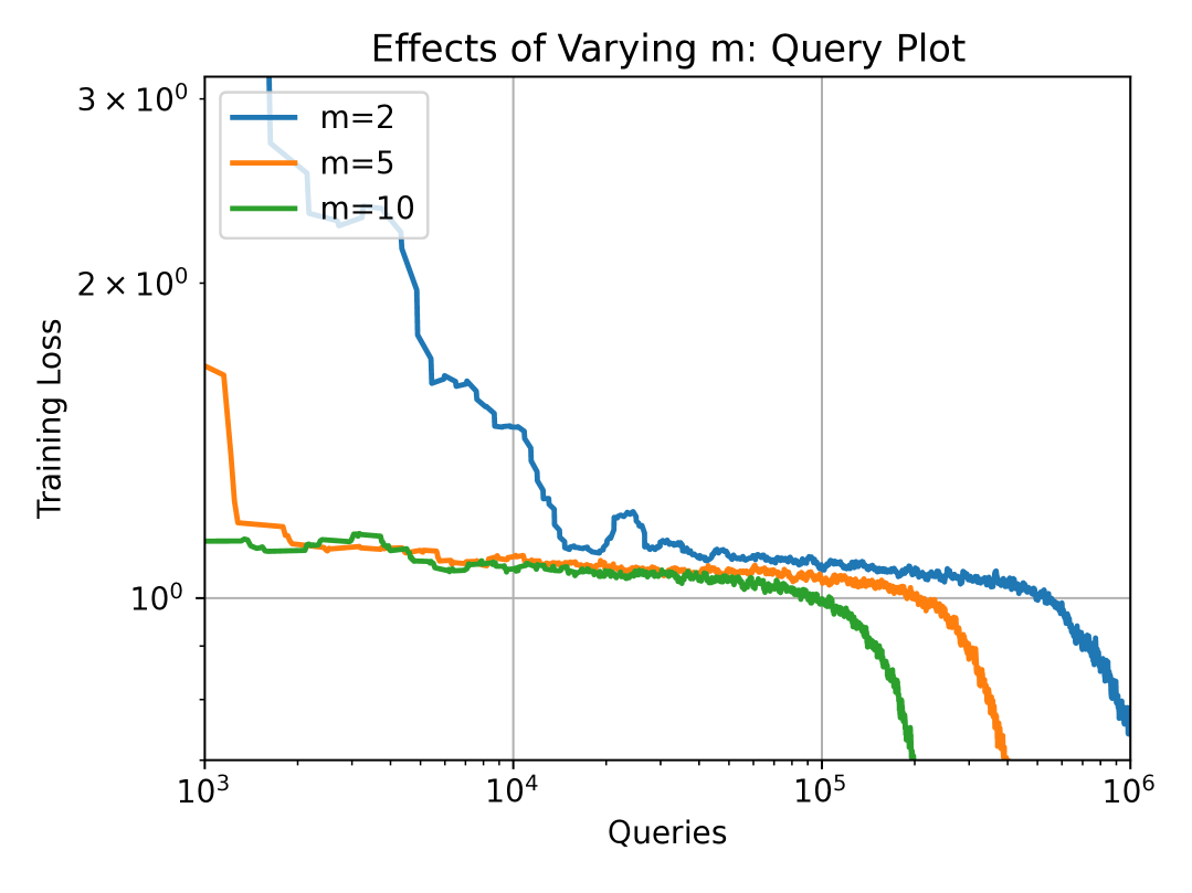
(c)

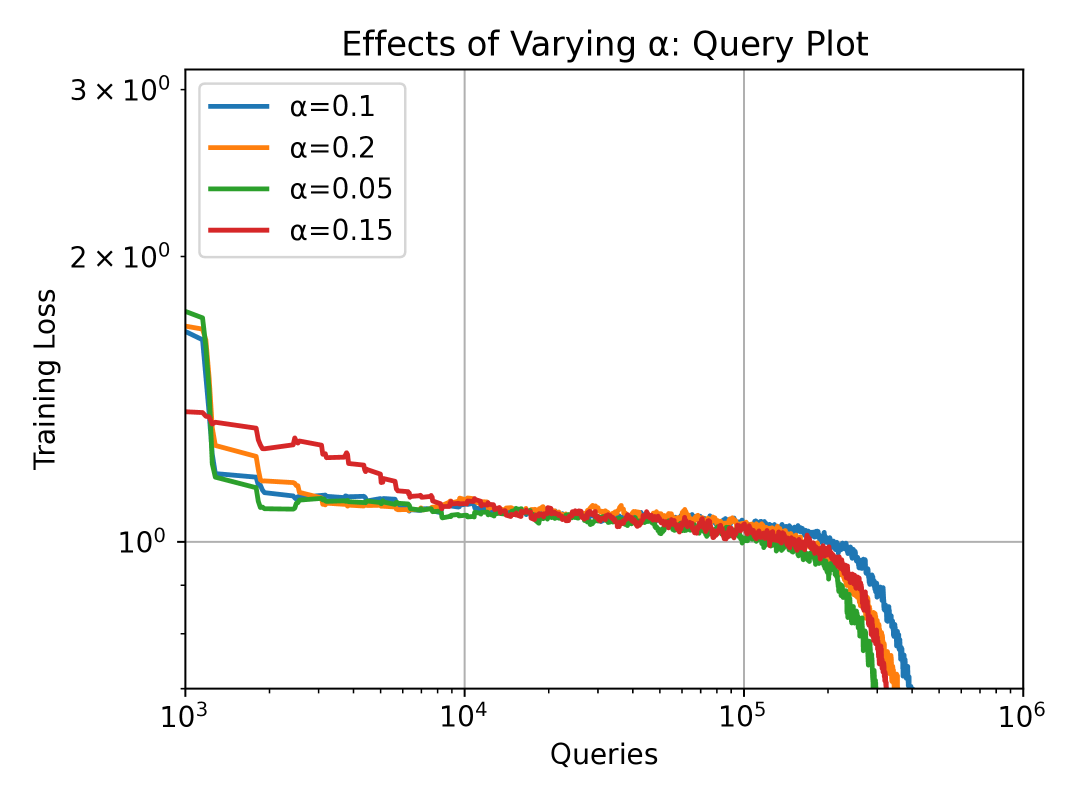
(d)

Figure 3: The effects of inner loop iterations $m$ and mixing coefficient $\alpha$ on the performance of VAMO for fine-tuning GPT-2 on MNLI.

References

- [1] Zeyuan Allen-Zhu and Yang Yuan. Improved svrg for non-strongly-convex or sum-of-non-convex objectives. In International conference on machine learning, pages 1080–1089. PMLR, 2016.
- [2] Sashank J Reddi, Ahmed Hefny, Suvrit Sra, Barnabas Poczos, and Alex Smola. Stochastic variance reduction for nonconvex optimization. In International conference on machine learning, pages 314–323. PMLR, 2016.
- [3] Rie Johnson and Tong Zhang. Accelerating stochastic gradient descent using predictive variance reduction. Advances in neural information processing systems, 26, 2013.
- [4] Yurii Nesterov and Vladimir Spokoiny. Random gradient-free minimization of convex functions. Foundations of Computational Mathematics, 17(2):527–566, 2017.
- [5] Sijia Liu, Bhavya Kailkhura, Pin-Yu Chen, Paishun Ting, Shiyu Chang, and Lisa Amini. Zeroth-order stochastic variance reduction for nonconvex optimization. Advances in neural information processing systems, 31, 2018.
- [6] Sadhika Malladi, Tianyu Gao, Eshaan Nichani, Alex Damian, Jason D Lee, Danqi Chen, and Sanjeev Arora. Fine-tuning language models with just forward passes. Advances in Neural Information Processing Systems, 36:53038–53075, 2023.
- [7] Tanmay Gautam, Youngsuk Park, Hao Zhou, Parameswaran Raman, and Wooseok Ha. Variance-reduced zeroth-order methods for fine-tuning language models. arXiv preprint arXiv:2404.08080, 2024.
- [8] John C Duchi, Michael I Jordan, Martin J Wainwright, and Andre Wibisono. Optimal rates for zero-order convex optimization: The power of two function evaluations. IEEE Transactions on Information Theory, 61(5):2788–2806, 2015.
- [9] Herbert Robbins and Sutton Monro. A stochastic approximation method. The annals of mathematical statistics, pages 400–407, 1951.
- [10] Robert M Gower, Mark Schmidt, Francis Bach, and Peter Richtárik. Variance-reduced methods for machine learning. Proceedings of the IEEE, 108(11):1968–1983, 2020.
- [11] Aaron Defazio, Francis Bach, and Simon Lacoste-Julien. Saga: A fast incremental gradient method with support for non-strongly convex composite objectives. Advances in neural information processing systems, 27, 2014.
- [12] Diederik P Kingma and Jimmy Ba. Adam: A method for stochastic optimization. arXiv preprint arXiv:1412.6980, 2014.
- [13] John Duchi, Elad Hazan, and Yoram Singer. Adaptive subgradient methods for online learning and stochastic optimization. Journal of machine learning research, 12(7), 2011.
- [14] Sashank J Reddi, Satyen Kale, and Sanjiv Kumar. On the convergence of adam and beyond. arXiv preprint arXiv:1904.09237, 2019.
- [15] Alexandre Défossez, Léon Bottou, Francis Bach, and Nicolas Usunier. A simple convergence proof of adam and adagrad. arXiv preprint arXiv:2003.02395, 2020.
- [16] Yushun Zhang, Congliang Chen, Naichen Shi, Ruoyu Sun, and Zhi-Quan Luo. Adam can converge without any modification on update rules. Advances in neural information processing systems, 35:28386–28399, 2022.
- [17] Yihua Zhang, Pingzhi Li, Junyuan Hong, Jiaxiang Li, Yimeng Zhang, Wenqing Zheng, Pin-Yu Chen, Jason D Lee, Wotao Yin, Mingyi Hong, et al. Revisiting zeroth-order optimization for memory-efficient llm fine-tuning: A benchmark. arXiv preprint arXiv:2402.11592, 2024.
- [18] Xinyu Tang, Ashwinee Panda, Milad Nasr, Saeed Mahloujifar, and Prateek Mittal. Private fine-tuning of large language models with zeroth-order optimization. arXiv preprint arXiv:2401.04343, 2024.
- [19] Zhenqing Ling, Daoyuan Chen, Liuyi Yao, Yaliang Li, and Ying Shen. On the convergence of zeroth-order federated tuning for large language models. In Proceedings of the 30th ACM SIGKDD Conference on Knowledge Discovery and Data Mining, pages 1827–1838, 2024.
- [20] Kevin G Jamieson, Robert Nowak, and Ben Recht. Query complexity of derivative-free optimization. Advances in Neural Information Processing Systems, 25, 2012.
- [21] Liu Liu, Minhao Cheng, Cho-Jui Hsieh, and Dacheng Tao. Stochastic zeroth-order optimization via variance reduction method. arXiv preprint arXiv:1805.11811, 2018.
- [22] Yining Wang, Simon Du, Sivaraman Balakrishnan, and Aarti Singh. Stochastic zeroth-order optimization in high dimensions. In International conference on artificial intelligence and statistics, pages 1356–1365. PMLR, 2018.
- [23] Pin-Yu Chen, Huan Zhang, Yash Sharma, Jinfeng Yi, and Cho-Jui Hsieh. Zoo: Zeroth order optimization based black-box attacks to deep neural networks without training substitute models. In Proceedings of the 10th ACM workshop on artificial intelligence and security, pages 15–26, 2017.
- [24] Chun-Chen Tu, Paishun Ting, Pin-Yu Chen, Sijia Liu, Huan Zhang, Jinfeng Yi, Cho-Jui Hsieh, and Shin-Ming Cheng. Autozoom: Autoencoder-based zeroth order optimization method for attacking black-box neural networks. In Proceedings of the AAAI conference on artificial intelligence, volume 33, pages 742–749, 2019.
- [25] Zeman Li, Xinwei Zhang, Peilin Zhong, Yuan Deng, Meisam Razaviyayn, and Vahab Mirrokni. Addax: Utilizing zeroth-order gradients to improve memory efficiency and performance of sgd for fine-tuning language models. arXiv preprint arXiv:2410.06441, 2024.
- [26] Saeed Ghadimi and Guanghui Lan. Stochastic first-and zeroth-order methods for nonconvex stochastic programming. SIAM journal on optimization, 23(4):2341–2368, 2013.
- [27] Yann N Dauphin, Razvan Pascanu, Caglar Gulcehre, Kyunghyun Cho, Surya Ganguli, and Yoshua Bengio. Identifying and attacking the saddle point problem in high-dimensional non-convex optimization. Advances in neural information processing systems, 27, 2014.
- [28] Krishnakumar Balasubramanian and Saeed Ghadimi. Zeroth-order nonconvex stochastic optimization: Handling constraints, high dimensionality, and saddle points. Foundations of Computational Mathematics, 22(1):35–76, 2022.
- [29] Sijia Liu, Pin-Yu Chen, Bhavya Kailkhura, Gaoyuan Zhang, Alfred O Hero III, and Pramod K Varshney. A primer on zeroth-order optimization in signal processing and machine learning: Principals, recent advances, and applications. IEEE Signal Processing Magazine, 37(5):43–54, 2020.
- [30] Huaiyi Mu, Yujie Tang, and Zhongkui Li. Variance-reduced gradient estimator for nonconvex zeroth-order distributed optimization. arXiv preprint arXiv:2409.19567, 2024.
- [31] James C Spall. Multivariate stochastic approximation using a simultaneous perturbation gradient approximation. IEEE transactions on automatic control, 37(3):332–341, 1992.
- [32] Abraham D Flaxman, Adam Tauman Kalai, and H Brendan McMahan. Online convex optimization in the bandit setting: gradient descent without a gradient. arXiv preprint cs/0408007, 2004.
- [33] Ohad Shamir. An optimal algorithm for bandit and zero-order convex optimization with two-point feedback. Journal of Machine Learning Research, 18(52):1–11, 2017.
- [34] Xiang Gao, Bo Jiang, and Shuzhong Zhang. On the information-adaptive variants of the admm: an iteration complexity perspective. Journal of Scientific Computing, 76:327–363, 2018.
- [35] Xiangru Lian, Huan Zhang, Cho-Jui Hsieh, Yijun Huang, and Ji Liu. A comprehensive linear speedup analysis for asynchronous stochastic parallel optimization from zeroth-order to first-order. Advances in neural information processing systems, 29, 2016.
- [36] Kaiyi Ji, Zhe Wang, Yi Zhou, and Yingbin Liang. Improved zeroth-order variance reduced algorithms and analysis for nonconvex optimization. In International conference on machine learning, pages 3100–3109. PMLR, 2019.
- [37] Yann LeCun, Léon Bottou, Yoshua Bengio, and Patrick Haffner. Gradient-based learning applied to document recognition. Proceedings of the IEEE, 86(11):2278–2324, 1998.
- [38] Alec Radford, Jeffrey Wu, Rewon Child, David Luan, Dario Amodei, Ilya Sutskever, et al. Language models are unsupervised multitask learners. OpenAI blog, 1(8):9, 2019.
- [39] Adina Williams, Nikita Nangia, and Samuel R Bowman. A broad-coverage challenge corpus for sentence understanding through inference. arXiv preprint arXiv:1704.05426, 2017.
- [40] Lihua Lei, Cheng Ju, Jianbo Chen, and Michael I Jordan. Non-convex finite-sum optimization via scsg methods. Advances in neural information processing systems, 30, 2017.