Capture and Escape of Planetary Mean-motion Resonances in Turbulent Discs

Abstract

Mean-motion resonances (MMRs) form through convergent disc migration of planet pairs, which may be disrupted by dynamical instabilities after protoplanetary disc (PPD) dispersal. This scenario is supported by recent analysis of TESS data showing that neighboring planet pairs in younger planetary systems are closer to resonance. To study stability of MMRs during migration, we perform hydrodynamical simulations of migrating planet pairs in PPDs, comparing the effect of laminar viscosity and realistic turbulence. We find stable 3:2 resonance capture for terrestrial planet pairs migrating in a moderately massive PPD, insensitive to a range of laminar viscosity ($\alpha=10^{-3}-10^{-1}$). However, realistic turbulence enhances overstability by sustaining higher equilibrium eccentricities and a positive growth rate in libration amplitude, ultimately leading to resonance escape. The equilibrium eccentricity growth rates decrease as planets migrate into tighter and more stable 4:3 and 5:4 MMRs. Our results suggest that active disc turbulence broadens the parameter space for overstability, causing planet pairs to end up in closer-in orbital separations. Libration within MMR typically lead to deviation from exact period ratio $|\Delta|\sim 0.5\%$, which alone is insufficient to produce the typical dispersion of $|\Delta|\sim 1-3\%$ in TESS data, suggesting that post-migration dynamical processes are needed to further amplify the offset.

1 Introduction

Orbital migration plays a crucial role in planet formation, ultimately shaping the architecture of planetary systems. Disc-driven migration occurs in the early stages of protoplanetary disc (PPD) evolution, when planets tidally interact with their natal discs. Type I migration primarily affects low-mass planets (Goldreich & Tremaine, 1980; Ward, 1997; Tanaka et al., 2002), typically up to a few Earth masses around Sun-like stars, before they reach the thermal mass to open up a gap in the disc (Lin & Papaloizou, 1986). This process influences the formation of super-Earths and proto-gas-giant cores (Ida & Lin, 2008; Benz et al., 2014; Liu et al., 2015). Migration torques, set by the disc structure (Paardekooper et al., 2010; Kley & Nelson, 2012; Paardekooper et al., 2023), usually leads to inward motion on a timescale shorter than the typical lifetime of PPDs. Recent studies have also found that additional physical processes, such as disc winds (McNally et al., 2017, 2018; Wu & Chen, 2025), dust feedback (Guilera et al., 2023; Hou & Yu, 2024, 2025), and background drift (Wu et al., 2024b), may also have the potential to modify the torques exerted on low-mass planets.

Mean-motion Resonances (MMRs) or resonant chains naturally arise from convergent migration of planet pairs (Lee & Peale, 2002) particularly when migration is relatively slow, though the exact conditions of resonant capture remain an active area of research (Goldreich & Schlichting, 2014; Huang & Ormel, 2023; Batygin & Petit, 2023; Wong & Lee, 2024; Lin et al., 2025; Keller et al., 2025). After PPD dispersal, these chains are expected to gradually break due to dynamical instabilities (Deck et al., 2013; Izidoro et al., 2017; Lammers et al., 2024), leading to late-stage compact systems that are typically not in resonance. The convergent migration scenario is supported by analysis of TESS data in Dai et al. (2024), who show that across an age spectrum, earlier planetary systems are more likely to be near-resonant.

Notably, these studies also find that observed period ratios often deviate from perfect commensurability by a fraction of $\Delta\sim$ from $-1\%$ to $3\%$, a feature also present in the Kepler catalogue (Fabrycky et al., 2014). This is commonly attributed to tidal dissipation after disc dispersal (Papaloizou & Terquem, 2010; Lithwick & Wu, 2012; Lee et al., 2013), though it has recently been suggested that the offset from the perfect period commensurability with a few percent could be attributed to the interference density wave when the planet pair is close to MMR (Yang & Li, 2024). However, the persistence of this $\Delta$ feature even in very young planetary systems, as emphasized by Dai et al. (2024), suggests that at least some fraction of this deviation may originate from migration itself. This is because producing such $\Delta$ by dissipation alone would require an unrealistically low total quality factor $Q$ (a measurement of material dissipation) for young planets (Xu & Dai, 2025).

This leads us to explore the possibility that planets may not be trapped in exact MMRs during convergent migration in the first place. The theory of resonant overstability, developed in the study of Saturnian satellites (Meyer & Wisdom, 2008), has been invoked by Goldreich & Schlichting (2014) as a potential explanation of non-negligible $\Delta$ during migration. Namely, when planet pairs migrate into MMRs, small perturbation in their eccentricities and period ratio evolves with time as $\propto\exp(s+i\omega)t$. Both the libration frequency $\omega$ and the growth rate $s$ are explicit functions of the equilibrium eccentricity $e_{\rm eq}$, which itself depends on the planet masses $M_{1},M_{2}$ and disc aspect ratio $h$. Analytical theory predicts that these oscillations are generally damped out ($s<0$) for planet-to-star mass ratio $q=M/M_{\star}\gtrsim h^{3}$, while $s>0$ for lower mass $q\lesssim h^{3}$, the latter leads to either (i) saturation towards an equilibrium libration amplitude, or (ii) escape out of resonance within an eccentricity damping timescale, and subsequent migration towards the next (closer-in) resonance. Disc dispersal during these librations will imprint such amplitudes into the current $\Delta$ distribution, even before the occurence of post-disc dynamical instabilities. This dichotomy is confirmed by recent hydrodynamic simulations of planet pairs migrating in and out of 2:1 resonances (Hands & Alexander, 2018; Ataiee & Kley, 2021; Afkanpour et al., 2024), although it’s worth noting that deviations from analytical theory can arise in low-viscosity cases due to partial gap-opening effects.

Nevertheless, as in classic simulation of planet migration in PPDs, turbulence is modeled as a laminar viscosity term that’s expected to solely enhance dissipation, damp waves and interference, and prevent gap-opening (e.g. Masset, 2000; Paardekooper et al., 2010; Kanagawa et al., 2015). Realistic turbulence from magneto-rotational instability (MRI) (Beckwith et al., 2011; Simon et al., 2012; Rea et al., 2024) and/or gravitational instability (GI) (Rice et al., 2003; Deng et al., 2017) present in PPDs, on the other hand, introduce trans-sonic scale turbulent eddies. These eddies could generate stochastic torques (Nelson, 2005; Wu et al., 2024a; Kubli et al., 2025) and excite oscillation from exact resonances, potentially influencing the equilibrium eccentricity $e_{\rm eq}$ as well as the growth rate $s$, which differs from laminar cases. The realistic effect of such turbulence on resonance capture remains to be studied by hydrodynamic simulations incorporating active turbulent prescriptions.

This paper is organized as follows: We introduce our numerical setup of modeling planet-disc interaction in §2 following Baruteau & Lin (2010); Chen & Lin (2023); Wu et al. (2024a). In §3, we present results from our simulations, focusing on the comparison between laminar viscosity versus active turbulence. In §4, we analyze equilibrium eccentricities and growth rates of perturbation at MMRs seen in our simulations under the Goldreich & Schlichting (2014) framework and conclude that active turbulence enhances both $e_{\rm eq}$ and $s$, favoring overstability. We discuss the implication of our findings and lay out future prospects in §5.

2 Numerical Setup

To explore multi-planet migration in PPDs, we use the hydrodynamic grid-based code FARGO3D (Benítez-Llambay & Masset, 2016), which is the successor of the FARGO code (Masset, 2000).

For our disc model, we set a locally isothermal disc with an aspect ratio $h\equiv H/r=h_{0}$, here the reference aspect ratio is $h_{0}=0.03$, consistent with most PPD models at close-in regions $<1$au (Garaud & Lin, 2007; Chiang & Youdin, 2010; Chiang & Laughlin, 2013; Chen et al., 2020). We also set the initial disc gas viscosity to be $\nu=\alpha H^{2}\Omega$ where $\alpha$ is a dimensionless parameter(Shakura & Sunyaev, 1973) and surface density profile to be $\Sigma=\Sigma_{0}(r/r_{0})^{-1/2}\left[M_{\star}/r_{0}^{2}\right]$, where $\Sigma_{0}$ is a normalization constant relevant to disc mass, $r_{0}$ is the code unit length and the initial inner planet’s orbital radius, $M_{\star}$ is the mass of the host star and the code unit for mass and $\Omega=\sqrt{GM_{\star}/r^{3}}$ is the Keplerian angular frequency. Because of the low disc masses considered in our simulations, we neglect self-gravity of the disc. The indirect term associated with the stellar motion is enabled (i.e., using the GASINDIRECTTERM option), as the star is fixed at the origin of the reference frame.

To model active turbulence for comparison against laminar $\alpha$, we modify the code with a phenomenological turbulence prescription (Laughlin et al., 2004; Baruteau & Lin, 2010; Chen & Lin, 2023; Wu et al., 2024a) to study planet migration in turbulent discs. We add a fluctuating potential $\Phi_{\rm turb}$ to the momentum equation consisted of 50 stochastic modes at each timestep:

$$\Phi_{\rm turb}(r,\phi,t)=\gamma r^{2}\Omega^{2}\sum_{k=1}^{50}\Lambda_{k}(m_{k},r,\varphi,t),$$ (1)

where $\gamma$ is a dimensionless characteristic amplitude of turbulence. Each mode, denoted as $\Lambda_{k}$, is given by

$$\Lambda_{k}=\xi_{k}e^{-(r-r_{k})^{2}/\sigma_{k}^{2}}\cos(m_{k}\phi-\phi_{k}-\Omega_{k}\tilde{t}_{k})\sin(\pi\tilde{t}_{k}/\Delta t_{k}),$$ (2)

which is associated with a wavenumber $m_{k}$ drawn from a logarithmically uniform distribution between $m=1$ and the maximum value $m_{\rm max}$ corresponding to azimuthal grid scale. The initial radial position $r_{k}$ and azimuthal angle $\phi_{k}$ of each mode are selected from a uniform distribution. The radial extent of each mode is $\sigma_{k}=\pi r_{k}/4m$. Modes activate at time $t_{0,k}$ and last for $\Delta t_{k}=0.2\pi r_{k}/mc_{s}$, where $c_{s}$ denotes the local sound speed. $\Omega_{k}$ represents the Keplerian frequency at $r_{k}$, $\tilde{t}_{k}=t-t_{0,k}$, and $\xi_{k}$ is a dimensionless constant sampled from a Gaussian distribution with unit width. Following Baruteau & Lin (2010), the parameter choices for this turbulence driver emulate a Kolmogorov cascade power spectrum, maintaining a $m^{-5/3}$ scaling law.

The relationship between $\gamma$ and the time-average effective Reynolds stress parameter $\langle\alpha_{R}\rangle$ (hereafter referred to as $\langle\alpha\rangle$) generated by this turbulence driver is calibrated to be (Baruteau & Lin, 2010; Chen & Lin, 2023; Wu et al., 2024a):

$$\langle\alpha\rangle\simeq 35(\gamma/h_{0})^{2}.$$ (3)

Although recent observational studies of line broadening have constrained the turbulence strength in nearby PPDs at large radial distances ($>30$ au) to be $\alpha<10^{-4}-10^{-3}$ (e.g., Flaherty et al., 2020; Lesur et al., 2023; Rosotti, 2023), turbulence level in the inner disc regions ($<1$ au) remains unclear due to limitations of current measurement techniques (Salyk et al., 2008; Romero-Mirza et al., 2024) and the possibility that existing observations may not be sensitive enough to detect viscous spreading (Alexander et al., 2023). Resolved observation Yound Stellar Object SVS 13 suggest that $\alpha\sim 10^{-2}$ at $\lesssim 0.3$au (Carr et al., 2004). Moreover, recent studies indicate that certain FU Ori-type outbursts can be explained by $\alpha\sim 0.03$ (Cleaver et al., 2023; Nayakshin et al., 2024), aligning with what we expect from theories of MRI when the temperature is high enough or when $\Sigma$ is low enough to be penetrated by cosmic rays (Gammie, 1996). In this study, we explore the range of $\langle\alpha\rangle$ between $10^{-3}$ to $10^{-1}$.

Our simulations are performed in a 2D $\left(r,\phi\right)$ coordinate system, with a computational domain ranging from 0.4 $r_{0}$ to 3.2 $r_{0}$ radially and 0 to $2\pi$ azimuthally. The domain is resolved by 512 logarithmic grid cells in the radial direction and 1536 grid cells in the azimuthal direction. We apply wave-damping radial boundary conditions (de Val-Borro et al., 2006), activating the KEPLERIAN2DDENS and STOCKHOLM options in FARGO3D. This setup is same as the Evanescent boundary conditions applied in Baruteau & Lin (2010) and Wu et al. (2024a). To avoid numerical issues caused by turbulence damping at the boundaries, we did not extend the turbulence across the entire disc but limit it to a radial range from 0.5 $r_{0}$ to 2.8 $r_{0}$.

In all simulations presented in this work, the planet system setup consists of Planet 1 (P1) initially positioned at an orbital radius of $r_{1}=1.0~r_{0}$ with a planet-to-stellar mass ratio of $q_{1}=5\times 10^{-6}$, and Planet 2 (P2) initially positioned at an orbital radius of $r_{2}=1.4~r_{0}$ (for laminar cases) or $1.35~r_{0}$ (for turbulent cases) with a planet-to-stellar mass ratio of $q_{2}=1.5\times 10^{-5}$. Both orbital separations lie just beyond the 3:2 MMR. The mass ratios correspond to $M_{1}=1.7M_{\oplus},M_{2}=5M_{\oplus}$ for a solar mass host star $M_{\star}=M_{\odot}$. We fully account for both planet-disc interaction and planet-planet interaction, allowing the planets to migrate freely.

As an indicator for MMR, during our runs we measure the inner planet’s (P1’s) resonant angle close to each $j:j+1$ order MMR as:

$$Q=(j+1)\lambda_{2}-j\lambda_{1}-\varpi_{1},$$ (4)

where $\lambda_{1}$ and $\varpi_{1}$ are mean longitude and longitude of pericenter of P1, and $\lambda_{2}$ is mean longitude of P2 (Murray & Dermott, 1999). For a stable resonance, $Q$ is expected to converge to some value close to $0$ or $\pi$ (Goldreich & Schlichting, 2014; Terquem & Papaloizou, 2019).

For each resonance, we generally consider planets to be trapped in resonance at $t_{\rm in}$ when the time evolution of period ratio $P_{2}/P_{1}$ flattens (a distinct transition, see §3). In some turbulent cases, we also consider planets to migrate out of resonance at $t_{\rm out}$ when $P_{2}/P_{1}$ deviates from commensurability by $>1\%$.

We measure the average equilibrium eccentricity $e_{\rm eq}$ for each resonance from $t_{\rm in}$ to $t_{\rm out}$ (or the end of the simulation, if we do not see resonance escape).

3 Results

3.1 Multi Planets Migration in Laminar Discs

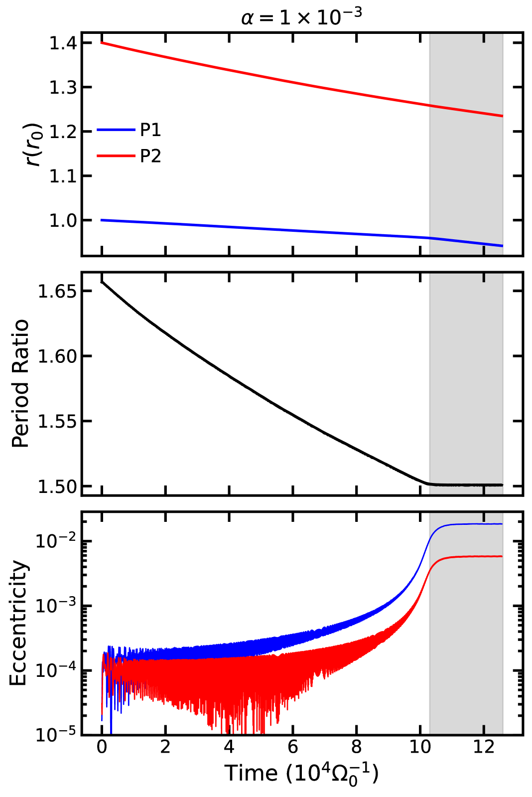
Figure 1: The three panels illustrate simulation results for our fiducial case (with $\alpha=1\times 10^{-3}$ and $\Sigma_{0}=2\times 10^{-5}$, as shown in the title). From top to bottom panel, we show time evolution of different orbital parameters: the radial positions of P1 (blue) and P2 (red); the period ratio between P1 and P2; the eccentricities of P1 and P2. The time axis is expressed in units of the dynamical timescale at P1’s initial position (i.e., $r_{p}=1r_{0}$). The two planets enters a 3:2 resonance state after approximately $t_{\rm in}=1.03\times 10^{5}\Omega_{0}^{-1}$ remained stable until the end of the simulation. Gray bands indicate the time “in resonance" during which we average $\langle e_{1}\rangle$ and $\langle e_{2}\rangle$.

We first present results from the fiducial laminar simulation with $\Sigma_{0}=2\times 10^{-5}$ and $\alpha=10^{-3}$. We show in Figure 1 the time evolution of a series of orbital parameters (from top to bottom: the semi-major axis, the period ratio, and the eccentricities $e$) obtained from our fiducial case. Using the dynamical timescale $\Omega_{0}^{-1}$ at P1’s initial position $r_{p}=1.0r_{0}$ as the reference time unit (which naturally arises from our choice of $G=M_{\star}=r_{0}$ as code unit), the planet pair enters a 3:2 MMR state after undergoing approximately $t_{\rm in}=1.03\times 10^{5}\Omega_{0}^{-1}\approx 1.65\times 10^{4}$ orbits of Type I migration. The system remains trapped in this resonance until the end of the simulation. During resonance, the planets’ eccentricities increase significantly by approximately two orders of magnitude, with the inner planet (P1) reaching as high as $\langle e_{1}\rangle=0.018$ and the outer planet (P2) $\langle e_{2}\rangle=0.006$. Note we have highlighted the time interval for performing time-averages of eccentricities from $t_{\rm in}$ to the end of simulation with gray shading in Figure 1. Figure 2 shows a typical surface density distribution snapshot during the 3:2 MMR in this simulation, where P2 causes a partial gap but gas depletion around the orbit of P1 is not significant. There are signs of interference between density waves generated by the planet pair. In Figure 3, we present the phase diagram of the time evolution of P1’s resonance angle for the fiducial case (with P1’s eccentricity as radial coordinate). It can be seen that the system remains at a fixed point for the resonance angle and eccentricity in the end of simulation without showing signs of overstability. The eccentricity $e_{1}$ converges to $\langle e_{1}\rangle$ and $\sin Q$ towards a small value $\ll 1$ (Goldreich & Schlichting, 2014). We have confirmed that the system is still trapped in the same fixed point when it evolves by further $3\times 10^{4}\Omega_{0}^{-1}$ without showing substantial change.

We also present the results of orbital parameters under higher laminar viscosity ($\alpha=1\times 10^{-1}$) in Figure 4. Overall, planets migrate slightly faster and the 3:2 MMR is reached earlier by $\sim 4000\Omega_{0}^{-1}\approx 600$ orbits compared to the $\alpha=1\times 10^{-3}$ case. Aside from this, the evolution of other orbital parameters closely resembles that of the fiducial simulation, confirming that equilibrium eccentricity and overstability in MMRs remain unaffected by viscosity as long as gap-opening is not significant and migration stays in the Type I regime (Afkanpour et al., 2024).

It is worth noting that our fiducial choice of $\Sigma_{0}$ guarantees a mild initial migration rate, allowing the planets to gradually become trapped in the 3:2 MMR. We show in Appendix A that planetary systems with more massive discs exhibit migration rates enhanced by approximately a factor of $\sim 5$, driving planets to bypass the 3:2 resonance configuration, consistent with theoretical expectations (Lin et al., 2025). Nevertheless, whether resonant planets escape MMR due to overstability is a separate issue independent of the capture criterion, the latter of which lies beyond the main scope of our paper.

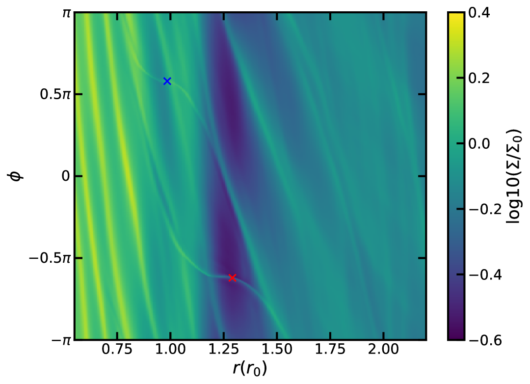
Figure 2: Typical surface density distribution for the fiducial case near the end of the simulation, where the planet pairs have captured into a 3:2 MMR. We use blue and red "x" symbols to indicate the positions of the inner (P1) and outer (P2) planets, respectively.

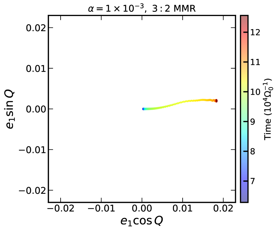
Figure 3: The time evolution of the resonant angle phase space of the inner planet for our fiducial model (laminar case with $\alpha=1\times 10^{-3}$, see in $\S$3.1) as the planet pairs migrate into the 3:2 resonance. Colour represents time.

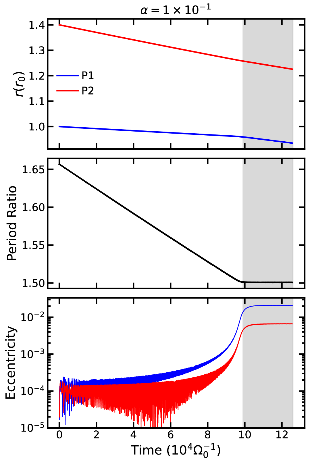
Figure 4: Similar to Figure 1, but for strong viscosity case (with $\alpha=1\times 10^{-1}$ and $\Sigma_{0}=2\times 10^{-5}$). The two planets entered a 3:2 resonance state after approximately $t_{\rm in}=9.7\times 10^{4}\Omega_{0}^{-1}$ and remained stable until the end of the simulation.

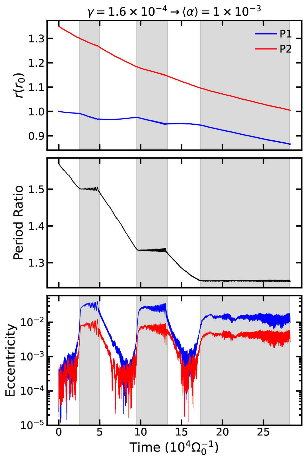
Figure 5: Similar to Figure 1, but for weak turbulent case (with $\gamma=1.6\times 10^{-4}$, corresponding to an effective viscosity stress parameter $\langle\alpha\rangle=1\times 10^{3}$). The planet pair traversed a total of three MMR states: 3:2, 4:3, and 5:4 and experienced two instances of resonance breaking.

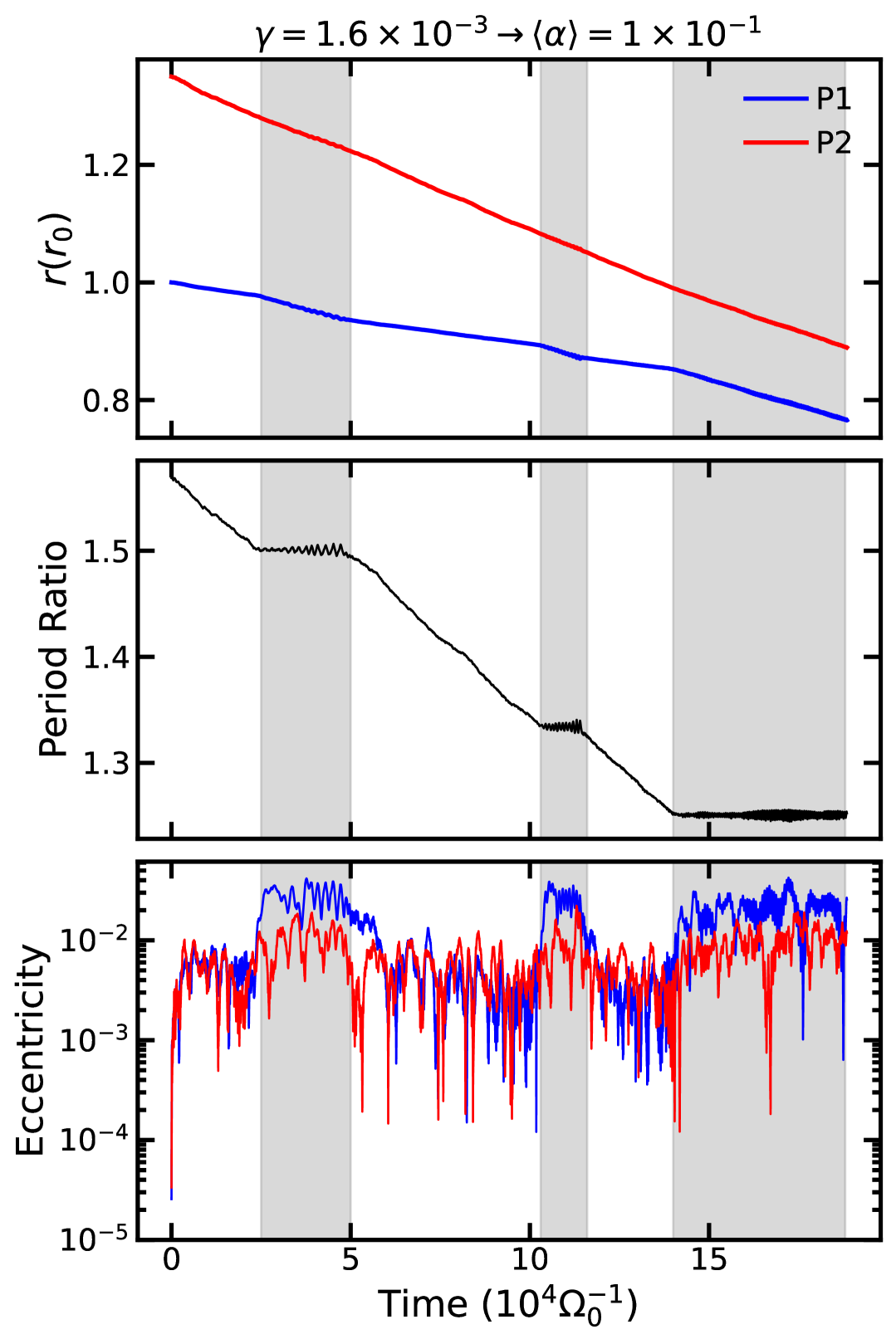
Figure 6: Similar to Figure 4, but for strong turbulent case (with $\gamma=1.6\times 10^{-3}$, corresponding to an effective viscosity stress parameter $\langle\alpha\rangle=1\times 10^{1}$). The planet pair traversed a total of three MMR states: 3:2, 4:3, and 5:4 and experienced two instances of resonance breaking.

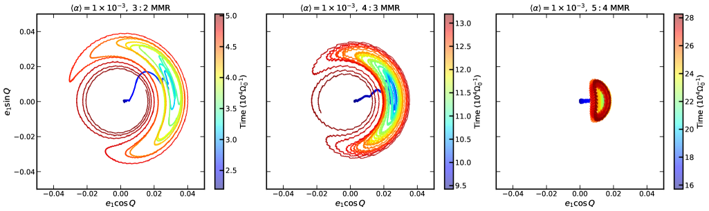
Figure 7: Time evolution of the resonance angle phase space of the inner planet for our weak turbulent model $\gamma=1.6\times 10^{-4}$. The three panels from left to right represent the periods when the planet pair become captured into (and escape out of, for unstable capture) the 3:2 MMR, 4:3 MMR, and 5:4 MMR, respectively.

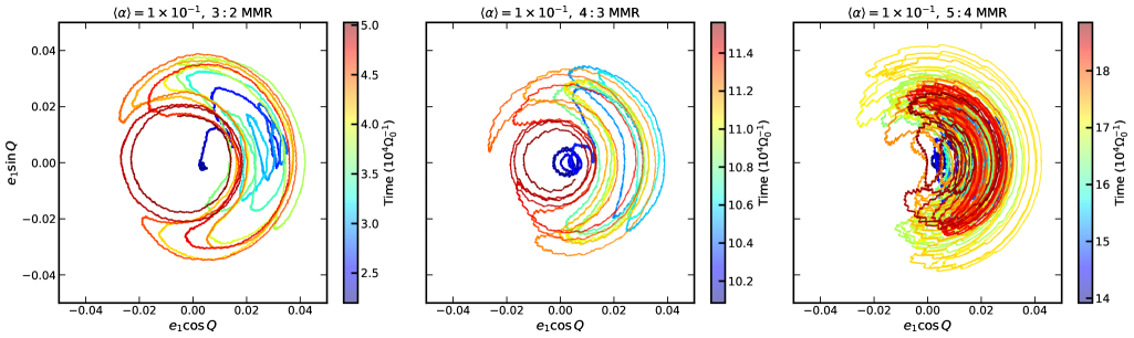
Figure 8: Similar to Figure 7, but for strongly turbulent case $\gamma=1.6\times 10^{-3}$.

3.2 Multi Planets Migration in Turbulent Discs

We proceed to present result from simulation of multi-planet migration in turbulent environment with the same initial disc mass $\Sigma_{0}=2\times 10^{-5}$. Scaling $r_{0}$ to radii within $\lesssim 0.3$ au, we expect MRI to be active through sublimation of alkali metals at high temperature (Desch & Turner, 2015). For $r_{0}\gtrsim 1$ au and $M_{\star}=M_{\odot}$, the column density corresponds to $\Sigma_{0}\lesssim 177$ g/cm², which is mariginaly sufficient condition for MRI activation via cosmic ray ionization (Gammie, 1996). As shown in Figure 5 and Figure 6, regardless of whether the turbulence level is weak (Figure 5, $\gamma=1.6\times 10^{-4}$, corresponding to effective $\langle\alpha\rangle=10^{-3}$) or strong (Figure 6, $\gamma=1.6\times 10^{-3}$, corresponding to effective $\langle\alpha\rangle=1\times 10^{-1}$), the planet pair undergoes multiple resonance escape events from 3:2, 4:3 to reach 5:4 at the end of our simulations. The behavior of each resonance escape aligns with semi-analytical studies of overstability in laminar discs (Goldreich & Schlichting, 2014), where small perturbations grow to a nonlinear amplitude before they resume their Type I migration and $P_{2}/P_{1}$ continues to linearly decrease. Similar to Figure 1, we highlight the time interval for each resonance from $t_{\rm in}$ to $t_{\rm out}$ (or end of our simulation) to indicate our averaging zones for eccentricities. The average values are recorded in Table 1.

For $\langle\alpha\rangle=10^{-3}$, the equilibrium eccentricity for 3:2 is larger than that for the laminar disc with similar effective $\alpha$ as shown in Figure 5. Furthermore, as evidenced by successive eccentricity plateaus in Figure 5, the equilibrium eccentricity progressively decreases with each successive resonance capture (indexed by $j$ for $j+1:j$ MMR) as the planets migrate inward, until the planets are trapped in 5:4 MMR from $t_{\rm in}\approx 1.7\times 10^{5}\Omega_{0}^{-1}$ till the end of simulation. Figure 7 shows the time evolution of the resonance angle for this simulation. For the 3:2 and 4:3 resonance, we observe eccentricity excitation when planet pair enters resonance, then quasi-periodic librations that eventually return to circulation when the pair escapes resonance. In contrast, the 5:4 MMR demonstrates significantly more confined motion, with the resonance angle eventually restricted to a much smaller region of phase space, suggesting a marginally stable resonant capture, as we would expect from the stronger mutual-interaction due to the closer distance between planets.

For $\langle\alpha\rangle=10^{-1}$, due to the presence of even higher levels of turbulence, the growth and decay of eccentricities become more chaotic and it’s hard to directly observe how $\langle e\rangle$ changes for each resonance from Figure 6 before time-averaging. At certain moments, the eccentricity of the outer planet even exceeds that of the inner planet. The evolution of resonance angle is also plotted in the right panel of Figure 8. However, the 5:4 MMR case shows a significant difference - unlike in the weak turbulence scenario, there is no sign of convergence in either eccentricity or resonance angle. Instead, the librations observed by the end of the simulation encompass the origin of the phase space, indicating a transition toward circulation. This implies that if the simulation time were extended, the planet pair in this case would eventually escape from the 5:4 MMR to even higher-order resonances.

Qualitatively, results from our turbulent simulations imply that active turbulence boosts overstability and helps planets overcome low $j$ MMRs and enter more closely-packed first-order resonances. In the next section, we will quantitatively show that positive overstability growth rate $s$ in these turbulent cases is consistent with the mild increase in $\langle e\rangle$ during MMRs.

4 Analysis

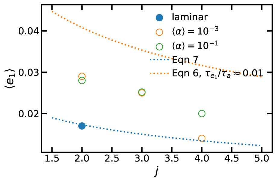
Figure 9: Measured average eccentricity of P1 during MMRs for all our simulations, plotted against estimate from the classical laminar context (blue dotted line), as well as combining Equation 6 with $\tau_{e_{1}}/\tau_{a}\sim 0.01$ (orange dotted line) as a rough estimate for turbulent cases.

In Figure 9, we plot P1’s average eccentricities during the resonances seen in our simulations (one 3:2 resonance for the laminar runs with nearly identical average $e_{1}$ for different $\alpha$, and three resonances for each turbulent run) in hollow circles (values are recorded in Table 1). In this way, we more clearly see the trend of $e_{1}$ decreasing with $j$ for turbulent cases, even though this trend is less significant for $\langle\alpha\rangle=10^{-1}$. In laminar discs context, for effective semi-major axis and eccentricity damping timescale of $\tau_{e},\tau_{a}$, Goldreich & Schlichting (2014); Huang & Ormel (2023) calculated the equilibrium eccentricity of the inner planet in a simplified restricted three-body problem (RTBP, assuming the outer planet is fixed and inner planet moves outwards into resonance on timescale of $\tau_{a_{1}}$) to be

$$e_{\rm eq,RTBP}^{2}={\dfrac{\tau_{e_{1}}}{2(j+1)\tau_{a_{1}}}}.$$ (5)

An analogous expression has also been obtained for tidally driven orbital migration and mean motion resonances of the Galilean satellites of Jupiter (Peale et al., 1979; Lin & Papaloizou, 1979).

The generalized expression for more realistic mutually-evolving planet pair migrating inwards is given by Terquem & Papaloizou (2019), which can be approximated to order-unity as

$$e_{\rm eq}^{2}={\dfrac{\tau_{e_{1}}}{2(j+1)\tau_{a}}},$$ (6)

where $\tau_{a}^{-1}:=|\dot{a}_{2}/a_{2}|-|\dot{a}_{1}/a_{1}|$ is the effective “approaching" timescale of two planets in the mutually evolving setup. Note that $e_{\rm eq}$ can be very close to $e_{\rm eq,RTBP}$ when $\dot{a}_{2}/a_{2}\sim 2\dot{a}_{1}/a_{1}$ as in our case, albeit the physical picture is slightly different. Since for the classic type I migration in the subsonic regime in laminar discs we expect $\tau_{e}/\tau_{a}\approx h^{2}$ (e.g. Papaloizou & Larwood, 2000; Tanaka et al., 2002; Li et al., 2019; Ida et al., 2020) regardless of $j$, Equation 5 or 6 may be approximated as

$$e_{\rm eq,laminar}^{2}\approx\dfrac{h^{2}}{j+1}.$$ (7)

For our laminar disc simulations, $j=2,h=0.03$ gives $e_{\rm eq,laminar}\approx 0.017$, which is very close to our measurement in both $\alpha=10^{-3}$ and $\alpha=10^{-1}$ simulations even if we do not explicitly invoke measurements of damping timescale. We plot $e_{\rm eq,laminar}$ across $j$ with a blue dotted line in Figure 9. For our turbulent cases, however, the eccentricities are systematically larger with stronger instability, and does not follow a $\propto(j+1)^{-1/2}$ decay as we might expect from a laminar disc.

To assess potential offsets in numerical measurements from expectations based on Equation 6, we need to provide some estimates of $\tau_{e}$ and $\tau_{a}$ for disc dissipation for our turbulent simulations. While it’s easy to average over the periods when planet pairs are undergoing Type I migration out of resonance to obtain $\tau_{a}\approx 4\times 10^{5}\Omega_{0}^{-1}$, measurement of $\tau_{e}$ is tricky since $\dot{e}/e$ can fluctuate very strongly when $e$ becomes negligible during Type I migration. The most reliable approach measuring $\tau_{e}$ is to average over a relatively short period $(\sim 10^{4}\Omega_{0}^{-1})$ right after $t_{\rm out}$, when eccentricity follows a nearly exponential decay and $\dot{e}/e$ is very well-defined (Hands & Alexander, 2018). Using this method, we measure $\tau_{e_{1}}\approx 4\times 10^{3}\Omega_{0}^{-1}$ for both runs, yielding an estimate of $\tau_{e_{1}}/\tau_{a}\sim 0.01$.

Finally, in Figure 9, we plot the theoretical equilibrium eccentricity by combining the measured value of $\tau_{e_{1}}/\tau_{a}\sim 0.01$ for turbulent discs with Equation 6 (orange dotted line). We see this could serve as an upper limit for theoretical estimate, though it may not be an accurate approximation. The overestimation compared to simulation result suggests that other non-linear effects may be providing feedback limiting the eccentricity, which implies that Equation 6 may not be able to capture all the dynamics of eccentricity excitation when active turbulence is present.

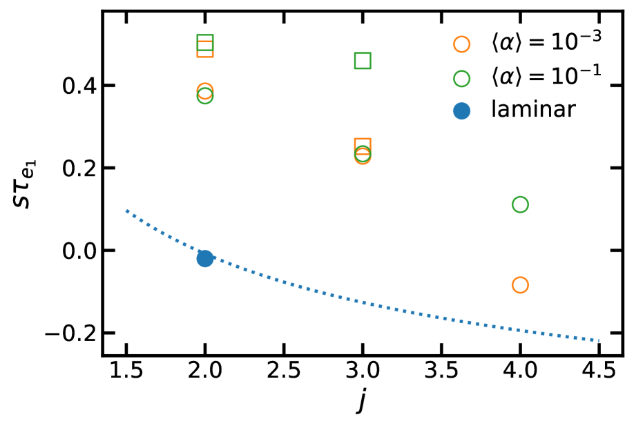
Figure 10: The dimensionless growth rate calculated from average eccentricity of P1 during MMRs for all our simulations, plotted against estimate from the classical laminar context (blue dotted line) which predicts laminar case to be stable. We also plot direct measurements for certain MMRs in square symbols.

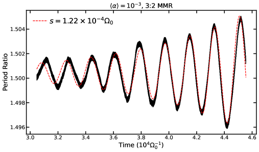
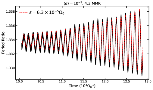
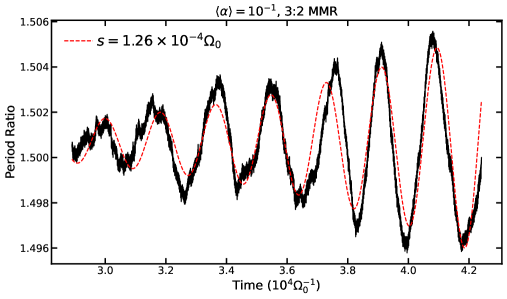
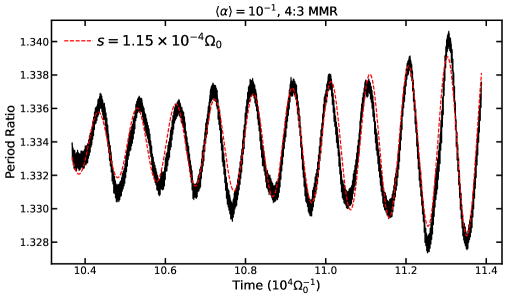
Figure 11: Best fits to the libration during MMRs with growth rates labeled for two turbulence runs.

In the RTBP approximation (Goldreich & Schlichting, 2014), linear perturbations in orbital parameters (e.g. eccentricity, period ratio) evolve with time as $\delta\propto\exp(s+i\omega)t$ when planets are in resonance, where

$$\omega/\Omega=\sqrt{3j^{2}f_{j}\tilde{\alpha}q_{2}e_{\rm eq}+\left(\dfrac{f_{j}\tilde{\alpha}q_{2}}{e_{\rm eq}}\right)^{2}},$$ (8)

and

$$s\tau_{e}=\left(\frac{\Omega}{\omega}\right)^{2}\left(3jf_{j}\tilde{\alpha}q_{2}e_{\mathrm{eq}}-\left(\frac{{f_{j}\tilde{\alpha}q_{2}}}{e_{\mathrm{eq}}}\right)^{2}\right).$$ (9)

Here $\tilde{\alpha}=(j/(j+1))^{2/3}$ is the semi-major axis ratio, and $f_{j}$ is an order-unity coefficients dependent on $j$ . One can see clearly that $s\tau_{e}$ is a sharply decreasing function of $e_{\mathrm{eq}}$.

We plot the predicted $s\tau_{e_{1}}$ in Figure 10 by substituting measured $\langle e_{1}\rangle$ into Equation 9 (corresponding to circles of similar color in Figure 9). To compare, we also plot the $s\tau_{e_{1}}$ profile calculated from Equation 7 expected for laminar discs, shown as the dotted blue line. We find that $s<0$ for $j\geq 2$, which suggests there will be no overstability as resonances become more and more stable for higher $j$. For turbulent cases, we see a systematic increase in $s$ solely due to larger $e_{\rm eq}$ values. This difference is sufficient to shift $s$ to positive values at $j=2,3$ for $\langle\alpha\rangle=10^{-3}$ and at all $j=2,3,4$ for $\langle\alpha\rangle=10^{-1}$.

Qualitatively, the sign change of expected $s\tau_{e_{1}}$ alone explains why turbulent cases are more prone to overstability, regardless of the value of $\tau_{e_{1}}$. To quantitatively compare with numerical results, we extract period ratio data from our turbulent runs during libration in MMRs and explicitly determine the perturbation growth rate. The exponential growth is apparent at least for the 3:2 and 4:3 resonances, where libration amplitude increases nearly monotonically (see black solid lines in Figure 11). However, it is not well-defined for the 5:4 MMR, where oscillation amplitude rises and falls chaotically towards the end of both simulations.

Simple Fourier transform for time evolution of period ratio during the 3:2 and 4:3 resonances will inform us that the peak libration frequency $\omega\sim 0.003\Omega_{0}$ for all cases, aligning with estimation from Equation 8 which is expected to be quite insensitive to $e_{\rm eq}$. However, measurement of $s$ this way is quite uncertain since the entire time series from capture to escape only spans roughly one e-folding timescale for the amplitude’s exponential growth (Goldreich & Schlichting, 2014), and Fourier spectrum becomes unreliable at low frequencies when the period approaches the total duration of the time series. We find it more straightforward to apply a nonlinear least-squares fit to the data, optimizing $\omega$ (which turns out to be consistent with results from Fourier transform) and $s$ jointly with the libration’s phase and amplitude. We plot best fits against data for 3:2 and 4:3 MMRs in our turbulent cases in Figure 11. We further multiply the values of best-fit $s$ by $\tau_{e_{1}}\sim 4\times 10^{3}\Omega_{0}^{-1}$ and plot the 4 “measured" values in Figure 10 with square symbols. By comparison, Equation 9 (circles) proves to be a sufficient approximation for $\langle\alpha\rangle=10^{-3}$ as long as we substitute in consistent measurements of equilibrium eccentricity. For $\langle\alpha\rangle=10^{-1}$, the values differs at 4:3 resonance by a factor of 2 but even so the measured $s$ still exhibits a decreasing trend with higher $j$. This suggests that, if migration continued indefinitely, the planets would ideally become stabilized in a much tighter resonance.

Finally, we note that no such measurements can be made for laminar cases as significant librations are absent. Nevertheless, the simple fact that the 3:2 MMR become stable is indeed consistent with $s<0$ for $j\geq 2$ along the blue dotted line in Figure 10.

Run	$\alpha=10^{-3}$	$\alpha=10^{-1}$	$\gamma=1.6\times 10^{-4}\rightarrow\langle\alpha\rangle=10^{-3}$			$\gamma=1.6\times 10^{-3}\rightarrow\langle\alpha\rangle=10^{-1}$
resonance	3:2	3:2	3:2	4:3	5:4	3:2	4:3	5:4
$\langle e_{1}\rangle$	0.018	0.018	0.029	0.025	0.014	0.028	0.025	0.020
$\langle e_{2}\rangle$	0.006	0.006	0.008	0.007	0.004	0.010	0.009	0.009

Table 1: Measured equilibrium eccentricity during MMRs for all our simulations.

5 Summary and Implications

In this paper, we apply hydrodynamical simulations of actively migrating planet pairs with laminar viscosity prescription versus active turbulence, to investigate the stability of first-order MMRs. In simulations with laminar viscosity $\alpha=10^{-3}-10^{-1}$, low-mass planet pairs become trapped into a perfect 3:2 resonance. With more realistic modeling of active turbulence, the 3:2 resonance becomes overstable. This overstability causes the period ratio and eccentricity to librate over time with a positive growth rate $s$ in amplitude, eventually resulting in resonance escape. The existence of these unstable modes $s>0$ are due to higher equilibrium eccentricities in a turbulent disc, albeit $s$ decreases as planets migrate into more stable, closer-in resonances, a trend that we also expect in classical theory for laminar discs. For effective $\langle\alpha\rangle=10^{-3}$, the planet pairs migrate past the 3:2 and 4:3 MMR, eventually stabilizing at the 5:4 MMR. For effective $\langle\alpha\rangle=10^{-1}$, even the 5:4 MMR would become unstable by the end of our simulation, and we expect the planet pair to eventually escape given sufficient time.

The direct conclusion from our analysis indicates that realistic turbulence expands the parameter space for overstability, causing planet pairs to migrate into tighter resonances compared to laminar discs. While we present the first hydrodynamic simulation for this comparison, a similar trend is observed in Izidoro et al. (2017, see their Figure 9), where effect of turbulence is modeled through a turbulent-potential prescription in their N-body simulations. However, such incorporation of turbulence in N-body simulations (Ogihara et al., 2007; Izidoro et al., 2017; Secunda et al., 2019) involves directly applying potential terms calibrated from simulations (Laughlin et al., 2004; Baruteau & Lin, 2010) (namely Equation 1) on the planets, which can be physically different from what is initially envisioned from the simulations: these potential terms are supposed to be applied to the disc gas to generate eddies in the surface density profile, mimicking the effects of effective Reynolds stress and the associated turbulent power spectrum. These eddies, in turn, influences the migration/damping torque exerted on the planets through modification of location and strength of Lindblad resonances. As we suggested in Wu et al. (2024a), a more realistic and straightforward way may be to apply stochastic torques (Rein & Papaloizou, 2009; Paardekooper et al., 2013; Hands et al., 2014), with dispersion as functions of disc parameters calibrated by turbulent simulations. Notably, a conclusion in Izidoro et al. (2017) is that the dichotomy between period ratio distribution in turbulent and laminar disc at the end of disc phase is small enough, such that it will be smeared out after reshaping of planet architecture by dynamical instability. Whether this relies on their specific treatment of turbulence remains to be investigated by updated population studies.

In terms of the deviation from commensurability,

$$\Delta:=\dfrac{P_{2}/P_{1}}{(j+1)/j}-1,$$ (10)

libration in our simulation typically results in $\Delta\sim 0.5\%$, which, although much larger than measured value for MMR in the laminar disc ($\Delta\sim 0.05\%$), is not enough to explain certain observed systems with $\Delta\sim 1-3\%$ (Dai et al., 2024) by itself. This value may serve as an adequate initial seed for resonant repulsion that eventually expands to values consistent with observation through post-PPD evolution (Xu & Dai, 2025) or other mechanisms (e.g., Papaloizou & Terquem, 2010; Lithwick & Wu, 2012; Batygin & Morbidelli, 2013; Delisle & Laskar, 2014; Choksi & Chiang, 2020). The prevalence of near-resonant planets in TESS systems close to 3:2 and 2:1 MMRs (Dai et al., 2024) may suggest low turbulence in their birth environments, with certain sources’ natal discs being quite laminar ($\Delta\sim 10^{-4}$), such as TOI-1136 (Dai et al., 2023), Kepler 60 and Kepler 223 (Fabrycky et al., 2014). Reversely, relatively lower occurence rate of planets near tighter (4:3 or 5:4) resonances does not necessarily indicate the scarcity of high-turbulence discs. Although these tighter resonances are more stable during migration, they are also more susceptible to resonance crossing and dynamical instability after disc dispersal (Lammers et al., 2024), which can disrupt MMRs. Nevertheless, some exceptions are emphasized by Li et al. (2024), who show that merger events due to dynamical instability might not eliminate near-resonant planet pairs but instead contribute to a moderate widening of $\Delta$ for surviving planets.

In a steady state, the accretion rate through the disc ${\dot{M}}_{d}=3\pi\Sigma\nu$ is independent of $r$. Normalized by the values of $h_{0}(=0.03)$ and $\Sigma_{0}(=2\times 10^{-5})$ we have adopted in the fiducial model,

$${\dot{M}}_{d}=2.7\times 10^{-8}\alpha\left({h_{0}\over 0.03}\right)^{2}\left({\Sigma_{0}\over 2\times 10^{-5}}\right)\left({M_{\star}\over M_{\odot}}{1~{\rm au}\over r_{0}}\right)^{3/2}{M_{\odot}\over{\rm yr}}.$$ (11)

Even with a relatively large $\alpha(\sim 0.1)$, the parameters used in the fiducial model are appropriate for the late stages of disc evolution around weak-line T Tauri stars. For the range of observed accretion rate onto classical T Tauri stars (Hartmann et al., 1998), larger values of $\Sigma_{0}$ are relevant. Such models may to lead more compact mean motion resonances (see the laminar model in Appendix A) between planets more massive than those simulated in the fiducial model. In a follow-up investigation, we will consider the possibility that, in turbulent discs around classical T Tauri stars, mean motion resonances between super-Earths may overlap with each other and the potential implications of resulting dynamical instability.

We also note that our treatment of active turbulence still differs from realistic MRI and GI generated from simulations incorporating magnetic fields and self-gravity (Simon et al., 2012; Deng et al., 2020). Analogous investigations of MMR capture and detachment in such environments are warranted and may not necessarily yield the same quantitative results. Nevertheless, our framework of comparing equilibrium eccentricity and growth rates of overstability during resonances with benchmark for analytical theory/laminar discs remains valuable.

Finally, we believe that with the upcoming operation of longer-baseline radio facilities in the coming decades, such as the Square Kilometre Array (SKA) and next generation Very Large Array (ngVLA), observational constraints on turbulence within PPDs and the ability to image substructures will continue to improve. These observations will help further constrain the turbulence strength in PPDs, particularly in the inner disc regions (Ricci et al., 2018; Wu et al., 2024c), and may even capture unusual substructures caused by planets migration or MMRs (Wu et al., 2023).

Data availability

The data obtained in our simulations can be made available on reasonable request to the corresponding author.

Appendix A Bypassing resonances in a heavier disc

In Figure 12, we present time evolution of orbital parameters for a laminar viscous simulation with $\alpha=10^{-3}$ and $\Sigma_{0}=10^{-4}[M_{\star}/r_{0}^{2}]$. We start with P2 at a semi-major axis of $1.65r_{0}$, and the planet pair migrated past both the 2:1 and 3:2 resonances without capture. For we can measure that $\tau_{a}\sim 10^{5}\Omega_{0}^{-1}$, shorter than the critical damping timescale required for slow-migration and capture into resonance (Lin et al., 2025):

$$\tau_{a,\rm crit}\approx\dfrac{1}{2(3j)^{1/3}}\dfrac{1}{(f_{j}\tilde{\alpha}q_{2})^{4/3}}\Omega_{0}^{-1},$$ (12)

which equals to $3.97\times 10^{5}\Omega_{0}^{-1}$ for 3:2 MMR and $1.26\times 10^{6}\Omega_{0}^{-1}$ for the much weaker 2:1 MMR. Therefore, resonance capture is unlikely in this laminar scenario due to rapid migration. Theoretically it could occur for $5:4$ MMR since $\tau_{a,\rm crit}$ decreases with $j$, but we do not extend our simulation longer to confirm as this is not the focus of our study. The value of $\tau_{a,\rm crit}$ at 3:2 MMR is consistent with our fiducial case, where the surface density is five times lower, resulting in a migration timescale approximately five times longer and satisfies the slow migration criterion.

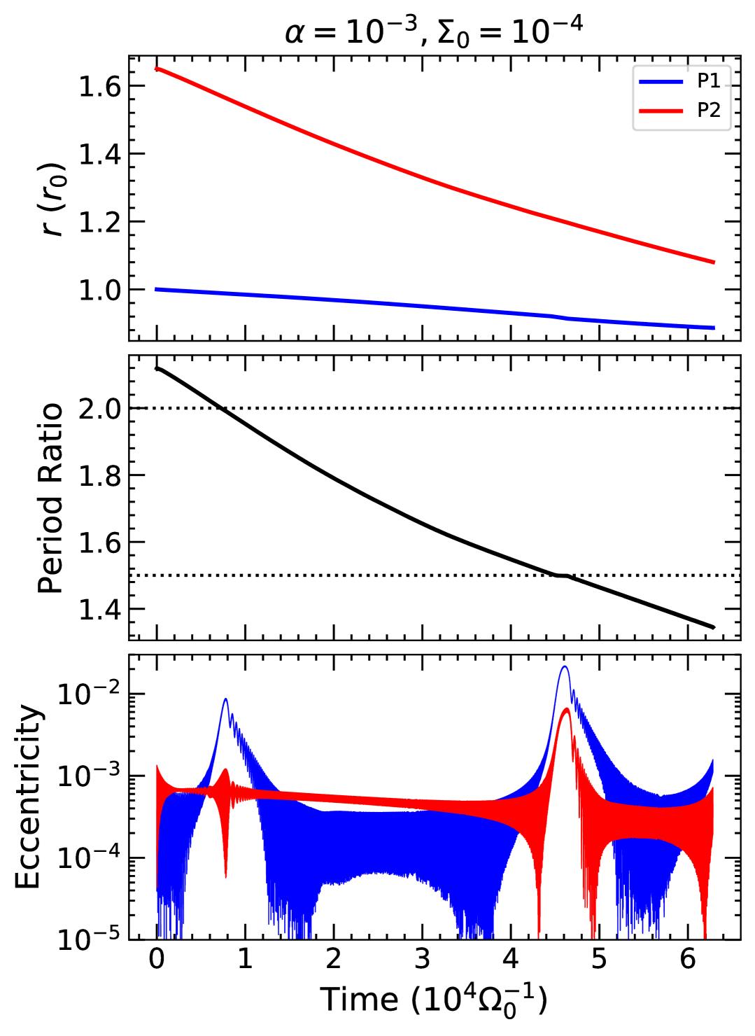
Figure 12: Orbital parameter evolution for additional laminar simulation with $\alpha=10^{-3}$ and $\Sigma_{0}=10^{-4}$. We demonstrate that planet pairs can migrate past the 2:1 and 3:2 MMR (dotted lines) without being captured when the migration speed is high due to a heavier disc.

References

- Afkanpour et al. (2024) Afkanpour Z., Ataiee S., Ziampras A., Penzlin A. B. T., Sfair R., Schäfer C., Kley W., Schlichting H., 2024, A&A, 686, A277
- Alexander et al. (2023) Alexander R., Rosotti G., Armitage P. J., Herczeg G. J., Manara C. F., Tabone B., 2023, MNRAS, 524, 3948
- Ataiee & Kley (2021) Ataiee S., Kley W., 2021, A&A, 648, A69
- Baruteau & Lin (2010) Baruteau C., Lin D. N. C., 2010, ApJ, 709, 759
- Batygin & Morbidelli (2013) Batygin K., Morbidelli A., 2013, AJ, 145, 1
- Batygin & Petit (2023) Batygin K., Petit A. C., 2023, ApJ, 946, L11
- Beckwith et al. (2011) Beckwith K., Armitage P. J., Simon J. B., 2011, MNRAS, 416, 361
- Benítez-Llambay & Masset (2016) Benítez-Llambay P., Masset F. S., 2016, ApJS, 223, 11
- Benz et al. (2014) Benz W., Ida S., Alibert Y., Lin D., Mordasini C., 2014, in Beuther H., Klessen R. S., Dullemond C. P., Henning T., eds, Protostars and Planets VI. pp 691–713 (arXiv:1402.7086), doi:10.2458/azu_uapress_9780816531240-ch030
- Carr et al. (2004) Carr J. S., Tokunaga A. T., Najita J., 2004, ApJ, 603, 213
- Chen & Lin (2023) Chen Y.-X., Lin D. N. C., 2023, MNRAS, 522, 319
- Chen et al. (2020) Chen Y.-X., Li Y.-P., Li H., Lin D. N. C., 2020, ApJ, 896, 135
- Chiang & Laughlin (2013) Chiang E., Laughlin G., 2013, MNRAS, 431, 3444
- Chiang & Youdin (2010) Chiang E., Youdin A. N., 2010, Annual Review of Earth and Planetary Sciences, 38, 493
- Choksi & Chiang (2020) Choksi N., Chiang E., 2020, MNRAS, 495, 4192
- Cleaver et al. (2023) Cleaver J., Hartmann L., Bae J., 2023, MNRAS, 523, 5522
- Dai et al. (2023) Dai F., et al., 2023, AJ, 165, 33
- Dai et al. (2024) Dai F., et al., 2024, AJ, 168, 239
- Deck et al. (2013) Deck K. M., Payne M., Holman M. J., 2013, ApJ, 774, 129
- Delisle & Laskar (2014) Delisle J. B., Laskar J., 2014, A&A, 570, L7
- Deng et al. (2017) Deng H., Mayer L., Meru F., 2017, ApJ, 847, 43
- Deng et al. (2020) Deng H., Mayer L., Latter H., 2020, ApJ, 891, 154
- Desch & Turner (2015) Desch S. J., Turner N. J., 2015, ApJ, 811, 156
- Fabrycky et al. (2014) Fabrycky D. C., et al., 2014, ApJ, 790, 146
- Flaherty et al. (2020) Flaherty K., et al., 2020, ApJ, 895, 109
- Gammie (1996) Gammie C. F., 1996, ApJ, 457, 355
- Garaud & Lin (2007) Garaud P., Lin D. N. C., 2007, ApJ, 654, 606
- Goldreich & Schlichting (2014) Goldreich P., Schlichting H. E., 2014, AJ, 147, 32
- Goldreich & Tremaine (1980) Goldreich P., Tremaine S., 1980, ApJ, 241, 425
- Guilera et al. (2023) Guilera O. M., Benitez-Llambay P., Miller Bertolami M. M., Pessah M. E., 2023, ApJ, 953, 97
- Hands & Alexander (2018) Hands T. O., Alexander R. D., 2018, MNRAS, 474, 3998
- Hands et al. (2014) Hands T. O., Alexander R. D., Dehnen W., 2014, MNRAS, 445, 749
- Hartmann et al. (1998) Hartmann L., Calvet N., Gullbring E., D’Alessio P., 1998, ApJ, 495, 385
- Hou & Yu (2024) Hou Q., Yu C., 2024, ApJ, 972, 152
- Hou & Yu (2025) Hou Q., Yu C., 2025, ApJ, 979, 185
- Huang & Ormel (2023) Huang S., Ormel C. W., 2023, MNRAS, 522, 828
- Ida & Lin (2008) Ida S., Lin D. N. C., 2008, ApJ, 673, 487
- Ida et al. (2020) Ida S., Muto T., Matsumura S., Brasser R., 2020, MNRAS, 494, 5666
- Izidoro et al. (2017) Izidoro A., Ogihara M., Raymond S. N., Morbidelli A., Pierens A., Bitsch B., Cossou C., Hersant F., 2017, MNRAS, 470, 1750
- Kanagawa et al. (2015) Kanagawa K. D., Tanaka H., Muto T., Tanigawa T., Takeuchi T., 2015, MNRAS, 448, 994
- Keller et al. (2025) Keller F., Dai F., Xu W., 2025, arXiv e-prints, p. arXiv:2504.12596
- Kley & Nelson (2012) Kley W., Nelson R. P., 2012, ARA&A, 50, 211
- Kubli et al. (2025) Kubli N., Mayer L., Deng H., Lin D. N. C., 2025, arXiv e-prints, p. arXiv:2503.01973
- Lammers et al. (2024) Lammers C., Hadden S., Murray N., 2024, ApJ, 972, 53
- Laughlin et al. (2004) Laughlin G., Steinacker A., Adams F. C., 2004, ApJ, 608, 489
- Lee & Peale (2002) Lee M. H., Peale S. J., 2002, ApJ, 567, 596
- Lee et al. (2013) Lee M. H., Fabrycky D., Lin D. N. C., 2013, ApJ, 774, 52
- Lesur et al. (2023) Lesur G., et al., 2023, in Inutsuka S., Aikawa Y., Muto T., Tomida K., Tamura M., eds, Astronomical Society of the Pacific Conference Series Vol. 534, Protostars and Planets VII. p. 465 (arXiv:2203.09821), doi:10.48550/arXiv.2203.09821
- Li et al. (2019) Li Y.-P., Li H., Li S., Lin D. N. C., 2019, ApJ, 886, 62
- Li et al. (2024) Li R., Chiang E., Choksi N., Dai F., 2024, arXiv e-prints, p. arXiv:2408.10206
- Lin & Papaloizou (1979) Lin D. N. C., Papaloizou J., 1979, MNRAS, 188, 191
- Lin & Papaloizou (1986) Lin D. N. C., Papaloizou J., 1986, ApJ, 309, 846
- Lin et al. (2025) Lin L., Liu B., Zheng Z., 2025, arXiv e-prints, p. arXiv:2501.12650
- Lithwick & Wu (2012) Lithwick Y., Wu Y., 2012, ApJ, 756, L11
- Liu et al. (2015) Liu B., Zhang X., Lin D. N. C., Aarseth S. J., 2015, ApJ, 798, 62
- Masset (2000) Masset F., 2000, A&AS, 141, 165
- McNally et al. (2017) McNally C. P., Nelson R. P., Paardekooper S.-J., Gressel O., Lyra W., 2017, MNRAS, 472, 1565
- McNally et al. (2018) McNally C. P., Nelson R. P., Paardekooper S.-J., 2018, MNRAS, 477, 4596
- Meyer & Wisdom (2008) Meyer J., Wisdom J., 2008, Icarus, 193, 213
- Murray & Dermott (1999) Murray C. D., Dermott S. F., 1999, Solar System Dynamics, doi:10.1017/CBO9781139174817.
- Nayakshin et al. (2024) Nayakshin S., Cruz Sáenz de Miera F., Kóspál Á., Ćalović A., Eislöffel J., Lin D. N. C., 2024, MNRAS, 530, 1749
- Nelson (2005) Nelson R. P., 2005, A&A, 443, 1067
- Ogihara et al. (2007) Ogihara M., Ida S., Morbidelli A., 2007, Icarus, 188, 522
- Paardekooper et al. (2010) Paardekooper S. J., Baruteau C., Crida A., Kley W., 2010, MNRAS, 401, 1950
- Paardekooper et al. (2013) Paardekooper S.-J., Rein H., Kley W., 2013, MNRAS, 434, 3018
- Paardekooper et al. (2023) Paardekooper S., Dong R., Duffell P., Fung J., Masset F. S., Ogilvie G., Tanaka H., 2023, in Inutsuka S., Aikawa Y., Muto T., Tomida K., Tamura M., eds, Astronomical Society of the Pacific Conference Series Vol. 534, Protostars and Planets VII. p. 685 (arXiv:2203.09595), doi:10.48550/arXiv.2203.09595
- Papaloizou & Larwood (2000) Papaloizou J. C. B., Larwood J. D., 2000, MNRAS, 315, 823
- Papaloizou & Terquem (2010) Papaloizou J. C. B., Terquem C., 2010, MNRAS, 405, 573
- Peale et al. (1979) Peale S. J., Cassen P., Reynolds R. T., 1979, Science, 203, 892
- Rea et al. (2024) Rea D. G., Simon J. B., Carrera D., Lesur G., Lyra W., Sengupta D., Yang C.-C., Youdin A. N., 2024, ApJ, 972, 128
- Rein & Papaloizou (2009) Rein H., Papaloizou J. C. B., 2009, A&A, 497, 595
- Ricci et al. (2018) Ricci L., Liu S.-F., Isella A., Li H., 2018, ApJ, 853, 110
- Rice et al. (2003) Rice W. K. M., Armitage P. J., Bate M. R., Bonnell I. A., 2003, MNRAS, 339, 1025
- Romero-Mirza et al. (2024) Romero-Mirza C. E., et al., 2024, ApJ, 964, 36
- Rosotti (2023) Rosotti G. P., 2023, New Astron. Rev., 96, 101674
- Salyk et al. (2008) Salyk C., Pontoppidan K. M., Blake G. A., Lahuis F., van Dishoeck E. F., Evans II N. J., 2008, ApJ, 676, L49
- Secunda et al. (2019) Secunda A., Bellovary J., Mac Low M.-M., Ford K. E. S., McKernan B., Leigh N. W. C., Lyra W., Sándor Z., 2019, ApJ, 878, 85
- Shakura & Sunyaev (1973) Shakura N. I., Sunyaev R. A., 1973, A&A, 24, 337
- Simon et al. (2012) Simon J. B., Beckwith K., Armitage P. J., 2012, MNRAS, 422, 2685
- Tanaka et al. (2002) Tanaka H., Takeuchi T., Ward W. R., 2002, ApJ, 565, 1257
- Terquem & Papaloizou (2019) Terquem C., Papaloizou J. C. B., 2019, MNRAS, 482, 530
- Ward (1997) Ward W. R., 1997, Icarus, 126, 261
- Wong & Lee (2024) Wong K. H., Lee M. H., 2024, AJ, 167, 112
- Wu & Chen (2025) Wu Y., Chen Y.-X., 2025, MNRAS, 536, L13
- Wu et al. (2023) Wu Y., Baruteau C., Nayakshin S., 2023, MNRAS, 523, 4869
- Wu et al. (2024a) Wu Y., Chen Y.-X., Lin D. N. C., 2024a, MNRAS, 528, L127
- Wu et al. (2024b) Wu Y., Lin M.-K., Cui C., Krapp L., Lee Y.-N., Youdin A. N., 2024b, ApJ, 962, 173
- Wu et al. (2024c) Wu Y., Liu S.-F., Jiang H., Nayakshin S., 2024c, ApJ, 965, 110
- Xu & Dai (2025) Xu Y., Dai F., 2025, ApJ, 981, 142
- Yang & Li (2024) Yang H., Li Y.-P., 2024, MNRAS, 534, 485
- de Val-Borro et al. (2006) de Val-Borro M., et al., 2006, MNRAS, 370, 529