Coupled Adaptable Backward-Forward-Backward Resolvent Splitting Algorithm (CABRA): A Matrix-Parametrized Resolvent Splitting Method for the Sum of Maximal Monotone and Cocoercive Operators Composed with Linear Coupling Operators

Abstract

We present a novel matrix-parametrized frugal splitting algorithm which finds the zero of a sum of maximal monotone and cocoercive operators composed with linear selection operators. We also develop a semidefinite programming framework for selecting matrix parameters and demonstrate its use for designing matrix parameters which provide beneficial diagonal scaling, allow parallelization, and adhere to a given communication structure. We show that taking advantage of the linear selection operators in this way accelerates convergence in numeric experiments, and show that even when the selection operators are the identity, we can accelerate convergence by using the matrix parameters to provide appropriately chosen diagonal scaling. We conclude by demonstrating the applicability of this algorithm to multi-stage stochastic programming, outlining a decentralized approach to the relaxed stochastic weapon target assignment problem which splits over the source nodes and has low data transfer and memory requirements.

1 Introduction

The applicability of matrix-parametrized (adaptable) frugal resolvent splittings to finding the zeros of the sum of finitely-many maximal monotone and cocoercive operators which are composed with bounded linear operators remains an open question in recent literature [1]. Our research develops a novel matrix-parametrized backward-forward-backward resolvent splitting algorithm which solves this problem when the bounded linear operators are selection operators. We prove the algorithm’s convergence, and provide a matrix parameter selection framework which allows us to optimize the matrix parameters to meet a wide range of objectives. These include finding matrix parameters which allow decentralized parallel execution, maximize the algebraic connectivity of the splitting, or provide diagonal scaling for the operators. In numerical experiments, we show that accounting for the selection operator structure accelerates convergence while reducing memory use and communication. These experiments also show that designing the matrix parameters in light of the expected operator output provides even greater improvements in convergence. We conclude by outlining the applicability of the algorithm to stochastic programming, developing a beneficial decentralized splitting structure for the continuous relaxation of the multi-stage stochastic weapon target assignment problem.

Coupled Inclusion Problem

We consider the following problem. Let $\mathcal{K}=\{1,\dots,p\}$, $\mathcal{I}=\{1,\dots,n\}$, and $\mathcal{J}=\{1,\dots,m\}$. Let $(\mathcal{G}_{k})_{k\in\mathcal{K}}$ be real Hilbert spaces. For all $i\in\mathcal{I}$, let $\mathcal{K}^{A}_{i}\subseteq\mathcal{K}$, $\mathcal{H}_{i}=\bigoplus_{k\in\mathcal{K}^{A}_{i}}\mathcal{G}_{k}$, $A_{i}:\mathcal{H}_{i}\rightrightarrows\mathcal{H}_{i}$ be a maximal monotone operator, and $R^{A}_{i}:\bigoplus_{k\in\mathcal{K}}\mathcal{G}_{k}\to\mathcal{H}_{i}$ be a selection operator which selects the subvectors given by $\mathcal{K}^{A}_{i}$, so that $R^{A}_{i}y=(y_{k})_{k\in\mathcal{K}^{A}_{i}}$. For all $j\in\mathcal{J}$, let $\mathcal{K}^{B}_{j}\subseteq\mathcal{K}$, $\mathcal{B}_{j}=\bigoplus_{k\in\mathcal{K}^{B}_{j}}\mathcal{G}_{k}$, and $B_{j}:\mathcal{B}_{j}\to\mathcal{B}_{j}$ be a $\beta_{j}$-cocoercive operator. Let $R^{B}_{j}:\bigoplus_{k\in\mathcal{K}}\mathcal{G}_{k}\to\mathcal{B}_{j}$ be a selection operator defined as $R^{B}_{j}y=(y_{k})_{k\in\mathcal{K}^{B}_{j}}$. We consider the following problem:

$$\text{find}\;y\in\bigoplus_{k\in\mathcal{K}}\mathcal{G}_{k}\;\text{such that}\;0\in\sum_{i=1}^{n}(R^{A}_{i})^{*}A_{i}R^{A}_{i}y+\sum_{j=1}^{m}(R^{B}_{j})^{*}B_{j}R^{B}_{j}y.$$ (1)

Algorithmic Approach

We define $n_{k}$ as the number of operators $A_{i}$ for which $k\in\mathcal{K}^{A}_{i}$ and assume $n_{k}\geq 2$ for all $k\in\mathcal{K}$. Let $\mathcal{H}_{\text{x}}=\bigoplus_{i=1}^{n}\mathcal{H}_{i}$, $\mathcal{B}_{\text{x}}=\bigoplus_{j=1}^{m}\mathcal{B}_{j}$, and $\mathcal{H}_{\text{z}}=\bigoplus_{k=1}^{m}\mathcal{G}_{k}^{n_{k}-1}$. For $x_{i}\in\mathcal{H}_{i}$, $x^{\prime}_{j}\in\mathcal{B}_{j}$, and $z_{k}\in\mathcal{G}_{k}^{n_{k}-1}$, we define the lifted variables $\mathbf{x}=(x_{i})_{i\in\mathcal{I}}\in\mathcal{H}_{\text{x}}$, $\mathbf{x}^{\prime}=(x^{\prime}_{j})_{j\in\mathcal{J}}\in\mathcal{B}_{\text{x}}$, and $\mathbf{z}=(z_{k})_{k\in\mathcal{K}}$. We define lifted operators $\mathbf{A}:\mathcal{H}_{\text{x}}\rightrightarrows\mathcal{H}_{\text{x}}$ and $\mathbf{B}:\mathcal{B}_{\text{x}}\to\mathcal{B}_{\text{x}}$ such that

$$\mathbf{A}\mathbf{x} =(A_{i}x_{i})_{i\in\mathcal{I}}$$ (2)

$$\mathbf{B}\mathbf{x}^{\prime} =(B_{j}x^{\prime}_{j})_{j\in\mathcal{J}}.$$ (3)

We select a set of bounded linear operators $\mathbf{D}_{A}:\mathcal{H}_{\text{x}}\to\mathcal{H}_{\text{x}}$, $\mathbf{L}_{A}:\mathcal{H}_{\text{x}}\to\mathcal{H}_{\text{x}}$, $\mathbf{M}_{A}:\mathcal{H}_{\text{x}}\to\mathcal{H}_{\text{z}}$, $\mathbf{Q}_{A}:\mathcal{B}_{\text{x}}\to\mathcal{H}_{\text{x}}$, and $\mathbf{K}_{A}:\mathcal{H}_{\text{x}}\to\mathcal{B}_{\text{x}}$ each as a permutation of a direct sum of $p$ linear operators which each meet a set of requirements given by . We then construct the Coupled Adaptable Backward-Forward-Backward Resolvent Splitting Algorithm (CABRA) by iterating over $\mathbf{z}$ as $\mathbf{z}^{\nu+1}=\mathbf{z}^{\nu}+\gamma\mathbf{M}_{A}\mathbf{x}$ where $\mathbf{x}$ is given by the resolvent

$$\mathbf{x}=J_{\alpha\mathbf{D}_{A}^{-1}\mathbf{A}}\left(\mathbf{D}_{A}^{-1}\left[-\mathbf{M}^{*}_{A}\mathbf{z}^{\nu}+2\mathbf{L}_{A}\mathbf{x}-\alpha\mathbf{Q}_{A}\mathbf{B}\mathbf{K}_{A}\mathbf{x}\right]\right).$$ (4)

We design $\mathbf{L}_{A}$ and $\mathbf{Q}_{A}\mathbf{B}\mathbf{K}_{A}$ to be strictly block lower triangular, so that can be found via forward substitution by iterating over the $n$ individual resolvents

$$x_{i}=J_{\alpha(\mathbf{D}_{A}^{-1})_{i}A_{i}}\left((\mathbf{D}_{A}^{-1})_{i}\left[-(\mathbf{M}^{*}_{A}\mathbf{z}^{k})_{i}+2\sum_{d=1}^{i-1}(\mathbf{L}_{A})_{id}x_{d}-\alpha b_{i}\right]\right)$$ (5)

where $b_{i}$ is a weighted sum of cocoercive operator outputs which depends only on $(x_{1},\dots,x_{i-1})$. Our algorithm generalizes the frugal resolvent splitting frameworks recently presented by Åkerman, Chenchene, Giselsson, and Naldi [1], and Dao, Tam, and Truong [11] which came to the attention of the authors as this work was being completed.

Paper Organization

We provide required background information and a literature review in Section 2. We then describe the proposed algorithm in detail and prove its convergence in Section 3. In Section 4, we show that the algorithm parameters can be found via a family of semi-definite programs, and conclude by providing a set of numerical examples and applications in Section 5.

2 Background

Following the publication of Ryu’s work on the uniqueness of Douglas-Rachford splitting as a frugal resolvent splitting (FRS) with minimal lifting [14], a large body of work has developed operator splitting algorithms with minimal lifting [12, 17, 13, 3, 4, 9, 10, 4, 5]. In [14], Ryu defines a resolvent splitting as a splitting constructed only with resolvents, scalar multiplication, and addition, and calls a resolvent splitting frugal if it evaluates each operator only once in each iteration. He also constructs a frugal three-operator resolvent splitting on $\mathcal{H}$ exhibiting minimal lifting, in that it lifts to $\mathcal{H}^{2}$ rather than $\mathcal{H}^{3}$. Malitsky and Tam generalize this in [12] to find an FRS with minimal lifting over $n$ operators, using matrices which correspond to a ring graph and a path graph which is its subset. These are generalized further into $d$-regular graphs in [17] and general unweighted graphs in [10], retaining the subgraph requirement in the latter case. The work in [7] demonstrates a semi-definite programming (SDP)-based approach to FRS matrix parameter selection which includes weighted graphs as well, and notes that the subgraph requirement is unnecessary.

The analysis in [13] extends the minimal lifting approach of Ryu and Malitsky and Tam to the summation of a set of maximal monotone and cocoercive operators, and [4] and [5] build ring and general graph-based frugal splittings with minimal lifting, respectively, in which the number of cocoercive operators is required to be less than the number of maximal monotone operators.

The recent work of Åkerman, Chenchene, Giselsson, and Naldi in [1] extends this broadly to define not only the sufficient conditions for the matrix parametrization, but also prove that these conditions are necessary for any frugal operator splitting over the summation of maximal monotone and cocoercive operators. A similar algorithm is given by the recent work of Dao, Tam, and Truong [11]. Algorithm 1 gives an independently developed variant of these algorithms, which this paper then extends to the more general case which includes the coupled linear selection operators.

2.1 Notation and Definitions

For $k\in\mathcal{K}$, let $\mathcal{G}_{k}$ be a real Hilbert space with inner product $\langle\cdot,\cdot\rangle$ and induced norm $\left\lVert\cdot\right\rVert$. We refer to $A$ as monotone if $\langle x-y,u-v\rangle\geq 0$ for all $(x,u)$ and $(y,v)$ in $\operatorname{graph}(A)=\{(x,u):u\in Ax\}$. It is maximal monotone if its graph is not properly contained in the graph of any other monotone operator. An operator $A$ is said to be $\beta$-cocoercive if $\langle x-y,Ax-Ay\rangle\geq\beta\left\lVert Ax-Ay\right\rVert^{2}$; we note that cocoercive operators are necessarily Lipschitz and single-valued. The resolvent of an operator $A$ is given by $J_{A}=(\mathrm{Id}+A)^{-1}$, where $\mathrm{Id}$ is the identity, and note that the resolvent of a maximal monotone operator is firmly nonexpansive and single-valued with full domain [8]. An operator $A$ is $\gamma$-averaged nonexpansive if

$$\left\lVert u-v\right\rVert^{2}\leq\left\lVert x-y\right\rVert^{2}-\frac{1-\gamma}{\gamma}\left\lVert(x-u)-(y-v)\right\rVert^{2}$$

for all $(x,u)$ and $(y,v)$ in $\operatorname{graph}(A)$. We write $\mathbb{S}_{+}^{n}$ for the set of symmetric $n\times n$ positive semi-definite (PSD) matrices, $\succeq$ for the generalized inequality on the PSD cone, and $\otimes$ for the Kronecker product. We denote lifted linear operators in bold, so for a matrix $M\in\mathbb{R}^{d\times n}$, $\mathbf{M}:\mathcal{H}^{n}\to\mathcal{H}^{d}$ is defined as $\mathbf{M}=M\otimes\mathrm{Id}$ where $\mathrm{Id}$ is the identity in $\mathcal{H}$. Bold vectors $\mathbf{x}$ exist within the lifted product space given at their definition. As in (2), other bold operators represent the direct sum of a set of operators on their respective lifted product space, where the product space $\bigoplus_{i=1}^{n}\mathcal{H}_{i}=\mathcal{H}_{1}\times\dots\times\mathcal{H}_{n}$ has the natural induced inner product and norm. We define $\text{tri}(Z)$ as the strict lower triangle of $Z$, and overload the diagonal notation so that $\operatorname{diag}(Z)$ returns the diagonal square matrix with the diagonal of $Z$ and zeros elsewhere when $Z$ is a square matrix and $\operatorname{diag}(x)$ returns the diagonal matrix with vector $x$ on the diagonal when $x$ is a vector.

2.2 Algorithm Parameter Assumptions

Similar to the development in [1] and other methods presented in the background section, the matrix parameters we use must satisfy a set of assumptions. However, unlike those methods, we will use these assumptions to develop $p$ separate sets of matrix parameters. For given dimensions $n^{\prime}$ and $m^{\prime}$ and cocoercivity parameter vector $\beta\in\mathbb{R}_{++}^{m^{\prime}}$, we choose $Z,W\in\mathbb{S}_{+}^{n^{\prime}}$, $K\in\mathbb{R}^{m^{\prime}\times n^{\prime}}$, and $Q\in\mathbb{R}^{n^{\prime}\times m^{\prime}}$, and derive $D,L\in\mathbb{R}^{n^{\prime}\times n^{\prime}}$, $M\in\mathbb{R}^{n^{\prime}-1\times n^{\prime}}$, and $U\in\mathbb{S}_{+}^{n^{\prime}}$ from $Z$, $W$, $K$, and $Q$ satisfying (6). We define $\bar{s}_{t}$ to be the maximum index in row $t$ of matrix $K$ such that $K_{ts}\neq 0$ and $\text{\@text@baccent{$s$}}_{t}$ to be the minimum index in column $t$ of matrix $Q$ such that $Q_{st}\neq 0$.

$$Z \succeq W$$ (6a)

$$Z \succeq U$$ (6b)

$$Z\mathbbm{1}_{n^{\prime}} =0$$ (6c)

$$D =\operatorname{diag}(Z)$$ (6d)

$$L =-\text{tri}(Z)$$ (6e)

$$\operatorname{null}(W) =\text{span}(\mathbbm{1}_{n^{\prime}})$$ (6f)

$$W =M^{\intercal}M$$ (6g)

$$U =(Q^{\intercal}-K)^{\intercal}\operatorname{diag}(\beta)^{-1}(Q^{\intercal}-K)$$ (6h)

$$K\mathbbm{1}_{n^{\prime}} =\mathbbm{1}_{m^{\prime}}$$ (6i)

$$Q^{\intercal}\mathbbm{1}_{n^{\prime}} =\mathbbm{1}_{m^{\prime}}$$ (6j)

$$\bar{s}_{t} <\text{\@text@baccent{$s$}}_{t}\quad t=1\dots m^{\prime}.$$ (6k)

Equations (6) imply that

$$D-L-L^{\intercal} =Z$$ (7a)

$$\mathbbm{1}_{n^{\prime}}^{\intercal}(D-2L)\mathbbm{1}_{n^{\prime}} =0$$ (7b)

$$U\mathbbm{1} =0$$ (7c)

$$\operatorname{null}(Z) =\text{span}(\mathbbm{1}_{n^{\prime}})$$ (7d)

$$\operatorname{null}(M) =\text{span}(\mathbbm{1}_{n^{\prime}}).$$ (7e)

For problem (1) with $p=1$ and $R^{A}_{i}=R^{B}_{j}=\mathrm{Id}$, these matrices define a valid splitting algorithm given by Algorithm 1, which is similar to the algorithms presented in [1] and [11], and is a special case of Algorithm 2. We assume here, and in Algorithm 2, that $\sum_{\nu=1}^{\infty}\gamma_{\nu}(2-\frac{\alpha}{2}-\gamma_{\nu})=\infty$.

Algorithm 1 Adaptable Backward-Forward-Backward Resolvent Splitting Algorithm

1:$\alpha\in(0,4)$; $\gamma_{\nu}\in(0,2-\frac{\alpha}{2})$; $\mathbf{z}^{0}\in\mathcal{G}^{n-1}$, $\mathbf{D}$, $\mathbf{M}$, $\mathbf{L}$, $\mathbf{Q}$, $\mathbf{K}$ satisfying (6).

2:$\nu\leftarrow 0$

3:repeat

4:  $\mathbf{x}^{\nu}=J_{\alpha\mathbf{D}^{-1}\mathbf{A}}\left(\mathbf{D}^{-1}\left[-\mathbf{M}^{*}\mathbf{z}^{\nu}+2\mathbf{L}\mathbf{x}^{\nu}-\alpha\mathbf{Q}\mathbf{B}\mathbf{K}\mathbf{x}^{\nu}\right]\right)$

5:  $\mathbf{z}^{\nu+1}=\mathbf{z}^{\nu}+\gamma_{\nu}\mathbf{M}\mathbf{x}^{\nu}$

6:  $\nu\leftarrow\nu+1$

7:until convergence

3 Coupled Adaptable Backward-Forward-Backward Resolvent Splitting

We now turn our attention to problem (1). We first describe the coupling operators $R^{A}_{i}$ and $R^{B}_{j}$ in more detail. Recall that $p$ gives the number of subvectors in the vector $y$, $\mathcal{K}^{A}_{i}$ gives the indices of the subvectors of $y$ which maximal monotone operator $A_{i}$ receives from $R^{A}_{i}$, and $\mathcal{K}^{B}_{j}$ gives the indices of the subvectors of $y$ which cocoercive operator $B_{j}$ receives from $R^{B}_{j}$. Therefore $R^{A}_{i}$ specifically returns the subvectors of $y$ which are in $\mathcal{H}_{i}=\bigoplus_{k\in\mathcal{K}^{A}_{i}}\mathcal{G}_{k}$, and similarly, $R^{B}_{j}$ returns only the subvectors of $y$ which are in $\mathcal{B}_{j}=\bigoplus_{k\in\mathcal{K}^{B}_{j}}\mathcal{G}_{k}$. We define the lifted coupling operators $\mathbf{R}_{A}:\bigoplus_{k\in\mathcal{K}}\mathcal{G}_{k}\to\mathcal{H}_{\text{x}}$ and $\mathbf{R}_{B}:\bigoplus_{k\in\mathcal{K}}\mathcal{G}_{k}\to\mathcal{B}_{\text{x}}$ as

$$\mathbf{R}_{A}y =(R^{A}_{i}y)_{i\in\mathcal{I}}$$ (8)

$$\mathbf{R}_{B}y =(R^{B}_{j}y)_{j\in\mathcal{J}}.$$ (9)

Operators $\mathbf{R}_{A}^{*}$ and $\mathbf{R}_{B}^{*}$ are the adjoint operators of $\mathbf{R}_{A}$ and $\mathbf{R}_{B}$ respectively with $\mathbf{R}_{A}^{*}\mathbf{A}\mathbf{x}$ returning a set containing $\mathbf{R}_{A}^{*}\mathbf{z}$ for each $\mathbf{z}\in\mathbf{A}\mathbf{x}$. With the definitions above, we can succinctly rewrite problem (1) as

$$\text{find}\;y\in\bigoplus_{k\in\mathcal{K}}\mathcal{G}_{k}\;\text{such that}\;0\in\mathbf{R}_{A}^{*}\mathbf{A}\mathbf{R}_{A}y+\mathbf{R}_{B}^{*}\mathbf{B}\mathbf{R}_{B}y.$$ (10)

3.1 Coupled Algorithm Matrices

We now discuss the lifting on $y$ and the determination of the matrix parameters. Let $\mathcal{I}_{k}$ be the ordered set of indices $i$ such that $k\in\mathcal{K}^{A}_{i}$. Let $s(i,k)$ give the index of $i$ in $\mathcal{I}_{k}$. Let $n_{k}=|\mathcal{I}_{k}|$, so that for each subvector $y_{k}$, $n_{k}$ gives the number of operators $A_{i}$ which operate on $y_{k}$. As previously noted, we assume that each subvector $y_{k}$ is an argument for at least two operators, so each $n_{k}\geq 2$. For each subvector $y_{k}$ of $y$, we form a lifted space $\mathcal{G}_{k}^{n_{k}}$. Let $\mathcal{H}_{\text{y}}=\bigoplus_{k\in\mathcal{K}}\mathcal{G}_{k}^{n_{k}}$. Let $\mathbf{y}\in\mathcal{H}_{\text{y}}$ be a lifted decision variable for $y$ grouped by subvector, with $\mathbf{y}_{k}\in\mathcal{G}_{k}^{n_{k}}$ and $\mathbf{y}_{ks}\in\mathcal{G}_{k}$ giving the $s$-th (sub-)subvector in $\mathbf{y}_{k}$ for $s\in\{1,\dots,n_{k}\}$.

Let $\mathcal{J}_{k}$ be the ordered set of indices $j$ such that $k\in\mathcal{K}^{B}_{j}$ and $m_{k}=|\mathcal{J}_{k}|$, so that for each subvector $y_{k}$, it gives the number of operators $B_{j}$ which operate on $y_{k}$. Note that unlike $n_{k}$, $m_{k}$ can equal zero. Let $t(j,k)$ give the index of $j$ in $\mathcal{J}_{k}$. Let $\mathcal{B}_{\text{y}}=\bigoplus_{k\in\bigcup_{j=1}^{m}\mathcal{K}^{B}_{j}}\mathcal{G}_{k}^{m_{k}}$, so that $\mathcal{G}_{k}$ is omitted if $m_{k}=0$. Let $\mathbf{y}^{\prime}\in\mathcal{B}_{\text{y}}$ be a lifted decision variable for $y$ grouped by subvector, with $\mathbf{y}^{\prime}_{k}\in\mathcal{G}_{k}^{m_{k}}$ and $\mathbf{y}^{\prime}_{kt}\in\mathcal{G}_{k}$ giving the $t$-th (sub-)subvector in $\mathbf{y}^{\prime}_{k}$ for $t\in\{1,\dots,m_{k}\}$ whenever $m_{k}\neq 0$.

Matrix Parameters

For each $k\in\mathcal{K}$, we use $n^{\prime}=n_{k}$, $m^{\prime}=m_{k}$, and

$$\beta_{k}=(\beta_{j})_{j\in\mathcal{J}_{k}}$$ (11)

to choose $Z_{k},W_{k}\in\mathbb{S}_{+}^{n_{k}}$, $Q_{k}\in\mathbb{R}^{n_{k}\times m_{k}}$, and $K_{k}\in\mathbb{R}^{m_{k}\times n_{k}}$ which together satisfy the assumptions in (6), as well as the matrices $D_{k}$, $L_{k}$, $M_{k}$, and $U_{k}$ which are derived from them. If $m_{k}=0$, we let $U_{k}=0$, $Q_{k}=0$, and $K_{k}=0$. Note that the requirement for $Z_{k}\succeq W_{k}\succeq 0$ and $\operatorname{null}(W_{k})=\text{span}(\mathbbm{1})$ in (6) imply that $D_{k}\succ 0$ and is therefore invertible. We choose $M_{k}\in\mathbb{R}^{n_{k}-1\times n_{k}}$ such that $M_{k}^{\intercal}M_{k}=W_{k}$, typically by Cholesky decomposition as described in [7]. We also require an additional condition to ensure that each cocoercive operator can receive all of its required input prior to the last opportunity for it to provide an output for each of its components. For each cocoercive operator $B_{j}$, let

$$\bar{i}_{j} =\max_{k\in\mathcal{K}^{B}_{j}}\min_{i\in\mathcal{I}_{k}}i$$ (12a)

$$\text{\@text@baccent{$i$}}_{j} =\min_{k\in\mathcal{K}^{B}_{j}}\max_{i\in\mathcal{I}_{k}}i,$$ (12b)

so that $\bar{i}_{j}$ gives the largest value of the initial entries in $\mathcal{I}_{k}$ for $k\in\mathcal{K}^{B}_{j}$ and $\text{\@text@baccent{$i$}}_{j}$gives the smallest value of the final entries in $\mathcal{I}_{k}$ for $k\in\mathcal{K}^{B}_{j}$. We assume that $\bar{i}_{j}<\text{\@text@baccent{$i$}}_{j}$ for all $j\in\mathcal{J}$, and select a cutoff operator index $i^{*}_{j}$ such that $\bar{i}_{j}\leq i^{*}_{j}<\text{\@text@baccent{$i$}}_{j}$. The cutoff operator $A_{i^{*}_{j}}$ is the last permissible source of inputs to cocoercive operator $B_{j}$. For each $j\in\mathcal{J}$ and $k\in\mathcal{K}^{B}_{j}$, let $s^{k}_{j}$ be the index of the last element in $\mathcal{I}_{k}$ which is less than or equal to $i^{*}_{j}$. We then require for each $K_{k}$ and $Q_{k}$ that

$$\bar{s}_{t(j,k)}\leq s^{k}_{j}<\text{\@text@baccent{$s$}}_{t(j,k)}\quad\forall j\in\mathcal{J}_{k}.$$ (13)

Our next step is to lift the matrices $Z_{k}$, $W_{k}$, $Q_{k}$, and $K_{k}$, and the matrices $D_{k}$, $L_{k}$, $M_{k}$, and $U_{k}$ derived from them, to operate on a lifted vector. We do so by constructing the bounded linear operator $\mathbf{Z}_{k}:\mathcal{G}_{k}^{n_{k}}\to\mathcal{G}_{k}^{n_{k}}$ as $\mathbf{Z}_{k}=Z_{k}\otimes\mathrm{Id}$, where $\mathrm{Id}$ is the identity operator on $\mathcal{G}_{k}$. Lifting the other operators in a similar fashion, we have the following collection of lifted operators:

$$\mathbf{Z}_{k} :\mathcal{G}_{k}^{n_{k}}\to\mathcal{G}_{k}^{n_{k}}\quad \mathbf{D}_{k} :\mathcal{G}_{k}^{n_{k}}\to\mathcal{G}_{k}^{n_{k}}$$ and (14)

$$\mathbf{Q}_{k} :\mathcal{G}_{k}^{m_{k}}\to\mathcal{G}_{k}^{n_{k}}\quad \mathbf{L}_{k} :\mathcal{G}_{k}^{n_{k}}\to\mathcal{G}_{k}^{n_{k}}$$

$$\mathbf{K}_{k} :\mathcal{G}_{k}^{n_{k}}\to\mathcal{G}_{k}^{m_{k}}\quad \mathbf{U}_{k} :\mathcal{G}_{k}^{n_{k}}\to\mathcal{G}_{k}^{n_{k}}$$

$$\mathbf{W}_{k} :\mathcal{G}_{k}^{n_{k}}\to\mathcal{G}_{k}^{n_{k}}\quad \mathbf{M}_{k} :\mathcal{G}_{k}^{n_{k}}\to\mathcal{G}_{k}^{n_{k}-1}.$$

Finally, we define the following lifted operators on $\mathcal{H}_{\text{y}}$ as the direct sum of their corresponding operators in (14):

$$\mathbf{Z} :\mathcal{H}_{\text{y}}\to\mathcal{H}_{\text{y}} \mathbf{Z}\mathbf{y} =(\mathbf{Z}_{k}\mathbf{y}_{k})_{k\in\mathcal{K}}$$ (15a)

$$\mathbf{D} :\mathcal{H}_{\text{y}}\to\mathcal{H}_{\text{y}} \mathbf{D}\mathbf{y} =(\mathbf{D}_{k}\mathbf{y}_{k})_{k\in\mathcal{K}}$$ (15b)

$$\mathbf{L} :\mathcal{H}_{\text{y}}\to\mathcal{H}_{\text{y}} \mathbf{L}\mathbf{y} =(\mathbf{L}_{k}\mathbf{y}_{k})_{k\in\mathcal{K}}$$ (15c)

$$\mathbf{W} :\mathcal{H}_{\text{y}}\to\mathcal{H}_{\text{y}} \mathbf{W}\mathbf{y} =(\mathbf{W}_{k}\mathbf{y}_{k})_{k\in\mathcal{K}}$$ (15d)

$$\mathbf{M} :\mathcal{H}_{\text{y}}\to\mathcal{H}_{\text{z}} \mathbf{M}\mathbf{y} =(\mathbf{M}_{k}\mathbf{y}_{k})_{k\in\mathcal{K}}$$ (15e)

$$\mathbf{U} :\mathcal{H}_{\text{y}}\to\mathcal{H}_{\text{y}} \mathbf{U}\mathbf{y} =(\mathbf{U}_{k}\mathbf{y}_{k})_{k\in\mathcal{K}}$$ (15f)

$$\mathbf{K} :\mathcal{H}_{\text{y}}\to\mathcal{B}_{\text{y}} \mathbf{K}\mathbf{y} =(\mathbf{K}_{k}\mathbf{y}_{k})_{k\in\bigcup_{j=1}^{m}\mathcal{K}^{B}_{j}}$$ (15g)

$$\mathbf{Q} :\mathcal{B}_{\text{y}}\to\mathcal{H}_{\text{y}} \mathbf{Q}\mathbf{y}^{\prime} =(\mathbf{Q}_{k}\mathbf{y}^{\prime}_{k})_{k\in\mathcal{K}}.$$ (15h)

We note that if $\mathbf{y}^{1}=\mathbf{Z}\mathbf{y}$, the subvector of $\mathbf{y}^{1}$ corresponding with $\mathcal{G}_{k}$ and $A_{i^{\prime}}$ for $i^{\prime}\in\mathcal{I}_{k}$ is given by $\mathbf{y}_{k,s(i^{\prime},k)}^{1}=\sum_{i\in\mathcal{I}_{k}}(Z_{k})_{s(i^{\prime},k),s(i,k)}\mathbf{y}_{k,s(i,k)}$.

Permutation Operators

We now define the permutation operators which allow us to work in $\mathcal{H}_{\text{x}}$ and $\mathcal{B}_{\text{x}}$ rather than $\mathcal{H}_{\text{y}}$ and $\mathcal{B}_{\text{y}}$. By definition, $\mathcal{H}_{\text{x}}=\bigoplus_{i=1}^{n}\mathcal{H}_{i}=\bigoplus_{i=1}^{n}\left(\bigoplus_{k\in\mathcal{K}^{A}_{i}}\mathcal{G}_{k}\right)$. The product space $\mathcal{H}_{\text{x}}$ therefore has $n_{k}$ copies of $\mathcal{G}_{k}$ for each $k\in\mathcal{K}$, just like $\mathcal{H}_{\text{y}}$, but grouped by operator, and therefore permuted by their appearance as arguments to operators $A_{i}$. We define the lifted operator $\mathbf{P}^{A}_{i}:\mathcal{H}_{\text{y}}\to\mathcal{H}_{i}$ as $\mathbf{P}^{A}_{i}\mathbf{y}=(\mathbf{y}_{k,s(i,k)})_{k\in\mathcal{K}^{A}_{i}}$, so that it selects from $\mathbf{y}$ the subvectors pertaining to operator $A_{i}$. The product space $\mathcal{B}_{\text{y}}$ also contains a permutation of the spaces $\mathcal{G}_{k}$ in $\mathcal{B}_{\text{x}}$, which also has $m_{k}$ copies of $\mathcal{G}_{k}$ for each $k\in\mathcal{K}$, with ordering determined by their order of appearance as arguments to operators $B_{j}$. We define the lifted operator $\mathbf{P}^{B}_{j}:\mathcal{B}_{\text{y}}\to\mathcal{B}_{j}$ as $\mathbf{P}^{B}_{j}\mathbf{y}^{\prime}=(\mathbf{y}^{\prime}_{k,t(j,k)})_{k\in\mathcal{K}^{B}_{j}}$, so that it selects from $\mathbf{y}^{\prime}$ the subvectors pertaining to operator $B_{j}$. We then define $\mathbf{P}_{A}$ and $\mathbf{P}_{B}$ as

$$\mathbf{P}_{A} :\mathcal{H}_{\text{y}}\to\mathcal{H}_{\text{x}} \mathbf{P}_{A}\mathbf{y} =(\mathbf{P}^{A}_{i}\mathbf{y})_{i\in\mathcal{I}}$$ (16a)

$$\mathbf{P}_{B} :\mathcal{B}_{\text{y}}\to\mathcal{B}_{\text{x}} \mathbf{P}_{B}\mathbf{y}^{\prime} =(\mathbf{P}^{B}_{j}\mathbf{y}^{\prime})_{j\in\mathcal{J}}.$$ (16b)

We note that, as permutation operators, the adjoints of $\mathbf{P}_{A}$ and $\mathbf{P}_{B}$, $\mathbf{P}_{A}^{*}:\mathcal{H}_{\text{x}}\to\mathcal{H}_{\text{y}}$ and $\mathbf{P}_{B}^{*}:\mathcal{B}_{\text{x}}\to\mathcal{B}_{\text{y}}$, are also the inverses of $\mathbf{P}_{A}$ and $\mathbf{P}_{B}$, respectively. We define $\mathcal{N}_{A}$ and $\mathcal{N}_{A}^{\perp}$ as

$$\mathcal{N}_{A} =\{\mathbf{x}\in\mathcal{H}_{\text{x}}:\exists y\in\bigoplus_{k\in\mathcal{K}}\mathcal{G}_{k}\,\text{where}\,\mathbf{x}=\mathbf{R}_{A}y\}$$ (17a)

$$\mathcal{N}^{\perp}_{A} =\{\mathbf{x}^{\perp}\in\mathcal{H}_{\text{x}}:\langle\mathbf{x}^{\perp},\mathbf{x}\rangle=0\quad\forall\mathbf{x}\in\mathcal{N}_{A}\}.$$ (17b)

Therefore, if $\mathbf{x}\in\mathcal{N}_{A}$ and $\mathbf{y}=\mathbf{P}_{A}^{*}\mathbf{x}$, we have $\mathbf{y}_{k}=\mathbbm{1}_{n_{k}}\otimes y_{k}$ for some $y_{k}\in\mathcal{G}_{k}$. Likewise, for $\mathbf{x}^{\perp}\in\mathcal{N}^{\perp}_{A}$ and $\mathbf{y}^{\perp}=\mathbf{P}_{A}^{*}\mathbf{x}^{\perp}$, we have

$$\langle\mathbbm{1}_{n_{k}},\mathbf{y}^{\perp}_{k}\rangle =0\quad\forall k\in\mathcal{K}$$ (18a)

$$\mathbf{R}_{A}^{*}\mathbf{x}^{\perp}=0.$$ (18b)

For $y\in\bigoplus_{k\in\mathcal{K}}\mathcal{G}_{k}$, $\mathbf{y}_{\mathbbm{1}}=(\mathbbm{1}_{n_{k}}\otimes y_{k})_{k\in\mathcal{K}}$, $\mathbf{y}^{\prime}_{\mathbbm{1}}=(\mathbbm{1}_{m_{k}}\otimes y_{k})_{k\in\bigcup_{j=1}^{m}\mathcal{K}^{B}_{j}}$, $\mathbf{x}\in\mathcal{H}_{\text{x}}$, and $\mathbf{x}^{\prime}\in\mathcal{B}_{\text{x}}$, we therefore have the following relationship between $\mathbf{P}_{A}$ and $\mathbf{R}_{A}$, and $\mathbf{P}_{B}$ and $\mathbf{R}_{B}$:

$$\mathbf{P}_{A}\mathbf{y}_{\mathbbm{1}} =\mathbf{R}_{A}y$$ (19a)

$$\mathbf{P}_{B}\mathbf{y}^{\prime}_{\mathbbm{1}} =\mathbf{R}_{B}y$$ (19b)

$$\langle\mathbbm{1}_{n_{k}},(\mathbf{P}_{A}^{*}\mathbf{x})_{k}\rangle =(\mathbf{R}_{A}^{*}\mathbf{x})_{k}$$ (19c)

$$\langle\mathbbm{1}_{m_{k}},(\mathbf{P}_{B}^{*}\mathbf{x}^{\prime})_{k}\rangle =(\mathbf{R}_{B}^{*}\mathbf{x}^{\prime})_{k}.$$ (19d)

Given the requirement for $K_{k}\mathbbm{1}_{n_{k}}=\mathbbm{1}_{m_{k}}$ and $Q_{k}^{\intercal}\mathbbm{1}_{n_{k}}=\mathbbm{1}_{m_{k}}$ in (6i) and (6j), we also have

$$\mathbf{y}^{\prime}_{\mathbbm{1}}=\mathbf{K}\mathbf{y}_{\mathbbm{1}} =\mathbf{K}\mathbf{P}_{A}^{*}\mathbf{R}_{A}y$$ (20a)

$$\mathbf{P}_{B}\mathbf{K}\mathbf{P}_{A}^{*}\mathbf{R}_{A}y =\mathbf{R}_{B}y$$ (20b)

$$\langle\mathbbm{1}_{n_{k}},(\mathbf{Q}\mathbf{P}_{B}^{*}\mathbf{x}^{\prime})_{k}\rangle =(\mathbf{R}_{B}^{*}\mathbf{x}^{\prime})_{k}.$$ (20c)

For ease of notation, we define the following compositions:

$$\mathbf{Z}_{A} :\mathcal{H}_{\text{x}}\to\mathcal{H}_{\text{x}} \mathbf{Z}_{A}\mathbf{x} =\mathbf{P}_{A}\mathbf{Z}\mathbf{P}_{A}^{*}\mathbf{x}$$ (21a)

$$\mathbf{D}_{A}^{-1} :\mathcal{H}_{\text{x}}\to\mathcal{H}_{\text{x}} \mathbf{D}_{A}^{-1}\mathbf{x} =\mathbf{P}_{A}\mathbf{D}^{-1}\mathbf{P}_{A}^{*}\mathbf{x}$$ (21b)

$$\mathbf{L}_{A} :\mathcal{H}_{\text{x}}\to\mathcal{H}_{\text{x}} \mathbf{L}_{A}\mathbf{x} =\mathbf{P}_{A}\mathbf{L}\mathbf{P}_{A}^{*}\mathbf{x}$$ (21c)

$$\mathbf{K}_{P} :\mathcal{H}_{\text{y}}\to\mathcal{B}_{\text{x}} \mathbf{K}_{P}\mathbf{y} =\mathbf{P}_{B}\mathbf{K}\mathbf{y}$$ (21d)

$$\mathbf{Q}_{P} :\mathcal{B}_{\text{x}}\to\mathcal{H}_{\text{y}} \mathbf{Q}_{P}\mathbf{x}^{\prime} =\mathbf{Q}\mathbf{P}_{B}^{*}\mathbf{x}^{\prime}$$ (21e)

$$\mathbf{K}_{A} :\mathcal{H}_{\text{x}}\to\mathcal{B}_{\text{x}} \mathbf{K}_{A}\mathbf{x} =\mathbf{K}_{P}\mathbf{P}_{A}^{*}\mathbf{x}$$ (21f)

$$\mathbf{Q}_{A} :\mathcal{B}_{\text{x}}\to\mathcal{H}_{\text{x}} \mathbf{Q}_{A}\mathbf{x}^{\prime} =\mathbf{P}_{A}\mathbf{Q}_{P}\mathbf{x}^{\prime}$$ (21g)

$$\mathbf{U}_{A} :\mathcal{H}_{\text{x}}\to\mathcal{H}_{\text{x}} \mathbf{U}_{A}\mathbf{x} =\mathbf{P}_{A}\mathbf{U}\mathbf{P}_{A}^{*}\mathbf{x}$$ (21h)

$$\mathbf{W}_{A} :\mathcal{H}_{\text{x}}\to\mathcal{H}_{\text{x}} \mathbf{W}_{A}\mathbf{x} =\mathbf{P}_{A}\mathbf{W}\mathbf{P}_{A}^{*}\mathbf{x}$$ (21i)

$$\mathbf{M}_{A} :\mathcal{H}_{\text{x}}\to\mathcal{H}_{\text{z}} \mathbf{M}_{A}\mathbf{x} =\mathbf{M}\mathbf{P}_{A}^{*}\mathbf{x}.$$ (21j)

The definition of $\mathbf{P}_{A}$ and $\mathcal{N}_{A}$, and the requirement for the null space of $W_{k}$ and $Z_{k}$ to be the ones vector, together imply that

$$\operatorname{null}(\mathbf{M}_{A}) =\operatorname{null}{(\mathbf{W}_{A})}=\operatorname{null}{(\mathbf{Z}_{A})}=\mathcal{N}_{A}$$ (22a)

$$\operatorname{ran}(\mathbf{M}^{*}_{A}) =\mathcal{N}_{A}^{\perp}$$ (22b)

$$(\mathbf{D}_{A}-2\mathbf{L}_{A})\mathbf{x} \in\mathcal{N}_{A}^{\perp}\quad\forall\mathbf{x}\in\mathcal{N}_{A}.$$ (22c)

Proofs of this are provided in Lemmas 6 and 7 in the appendix.

Algorithm Definition

We now introduce the fixed point iteration which defines Algorithm 2. Let the operators $T:\mathcal{H}_{\text{z}}\to\mathcal{H}_{\text{z}}$ and $S:\mathcal{H}_{\text{z}}\to\mathcal{H}_{\text{x}}$ be given by

$$S(\mathbf{z}) =-\left(\mathbf{D}_{A}-2\mathbf{L}_{A}+\alpha\mathbf{A}+\alpha\mathbf{Q}_{A}\mathbf{B}\mathbf{K}_{A}\right)^{-1}\mathbf{M}^{*}_{A}\mathbf{z}$$ (23a)

$$T(\mathbf{z}) =\left(\mathrm{Id}+\gamma\mathbf{M}_{A}S\right)(\mathbf{z}).$$ (23b)

Algorithm 2 CABRA: Coupled Adaptable Backward-Forward-Backward Resolvent Splitting Algorithm

1:$\alpha\in(0,4)$; $\gamma_{\nu}\in(0,2-\frac{\alpha}{2})$; $\mathbf{z}^{0}\in\bigoplus_{k\in\mathcal{K}}\mathcal{G}_{k}^{n_{k}-1}$; $\mathbf{D}_{A}^{-1}$, $\mathbf{M}_{A}$, $\mathbf{L}_{A}$, $\mathbf{Q}_{A}$, $\mathbf{K}_{A}$ satisfying (21).

2:$\nu\leftarrow 0$

3:repeat

4:  Solve $\mathbf{x}^{\nu}=J_{\alpha\mathbf{D}_{A}^{-1}\mathbf{A}}\left(\mathbf{D}_{A}^{-1}\left[-\mathbf{M}^{*}_{A}\mathbf{z}^{\nu}+2\mathbf{L}_{A}\mathbf{x}^{\nu}-\alpha\mathbf{Q}_{A}\mathbf{B}\mathbf{K}_{A}\mathbf{x}^{\nu}\right]\right)$

5:  $\mathbf{z}^{\nu+1}=\mathbf{z}^{\nu}+\gamma_{\nu}\mathbf{M}_{A}\mathbf{x}^{\nu}$

6:  $\nu\leftarrow\nu+1$

7:until convergence

This is equivalent to $T(\mathbf{z})=\mathbf{z}+\gamma\mathbf{M}_{A}\mathbf{x}$ where $\mathbf{x}$ is defined as in Algorithm 2 step (4). We show in Lemma 4 in the appendix that the permutation $\mathbf{P}_{A}$ preserves the ordering of the operators within each $L_{k}$, making $\mathbf{L}_{A}$ strictly block lower triangular so that $(\mathbf{L}_{A}\mathbf{x})_{i}$ depends only on $(x_{1},\dots,x_{i-1})$. Lemma 5 in the appendix similarly shows that the structure imposed on $Q_{k}$ and $K_{k}$ by the cutoff values $i^{*}_{j}$ with requirements (6k) and (13) mean that $(\mathbf{Q}_{A}\mathbf{B}\mathbf{K}_{A}\mathbf{x})_{i}$ also depends only on $(x_{1},\dots,x_{i-1})$. Therefore $\mathbf{x}$ in (4) is well-defined, and can be found by iteratively finding $J_{\alpha(\mathbf{D}_{A}^{-1})_{i}A_{i}}$ via forward substitution, working in parallel when any set of resolvents have all the input required by $\mathbf{L}_{A}$ and $\mathbf{Q}_{A}\mathbf{B}\mathbf{K}_{A}$.

3.2 Proof of convergence

We now proceed to prove the convergence of Algorithm 2. We begin by showing the correspondence between fixed points of $T$ and zeros of problem (1). We then establish a result linking the operator $\mathbf{Q}_{P}\mathbf{B}\mathbf{K}_{P}$ to $\mathbf{U}$ (and therefore to $\mathbf{Z}$ and $\mathbf{W}$), which will be necessary for establishing the nonexpansivity of $T$. This connection allows us to then show the $\gamma$-averaged nonexpansivity of $T$. Given this $\gamma$-averaged nonexpansivity, we then proceed to show that the existence of a zero is sufficient for weak convergence of the iterates $(\mathbf{z}^{k})$, and that the corresponding series $(\mathbf{x}^{k})$ weakly converges to a point $\mathbf{x}^{*}\in\mathcal{N}_{A}$ which corresponds with a solution to (1).

Our first lemma establishes the correspondence between the existence of a zero for problem (1) and the existence of a fixed point of $T$.

Lemma 1.

The set of fixed points of $T$ is non-empty if and only if the set of solutions to problem (1) is non-empty. That is,

$$y\in\mathrm{zer}\left(\mathbf{R}_{A}^{*}\mathbf{A}\mathbf{R}_{A}+\mathbf{R}_{B}^{*}\mathbf{B}\mathbf{R}_{B}\right)\iff\mathbf{z}\in\mathrm{Fix}(T),\mathbf{R}_{A}y=S\mathbf{z}.$$ (24)

Proof.

If $y\in\mathrm{zer}\left(\mathbf{R}_{A}^{*}\mathbf{A}\mathbf{R}_{A}+\mathbf{R}_{B}^{*}\mathbf{B}\mathbf{R}_{B}\right)$, then there exists a corresponding lifted $\mathbf{y}_{\mathbbm{1}}\in\mathcal{H}_{\text{y}}$, $\mathbf{x},\mathbf{w}\in\mathcal{H}_{\text{x}}$, and $\mathbf{x}^{\prime},\mathbf{u}\in\mathcal{B}_{\text{x}}$ such that

$$\mathbf{x} =\mathbf{R}_{A}y=\mathbf{P}_{A}\mathbf{y}_{\mathbbm{1}}$$ (25a)

$$\mathbf{x}^{\prime} =\mathbf{R}_{B}y=\mathbf{P}_{B}\mathbf{K}\mathbf{y}_{\mathbbm{1}}=\mathbf{K}_{A}\mathbf{x}$$ (25b)

$$\mathbf{w} \in\mathbf{A}\mathbf{x}$$ (25c)

$$\mathbf{u} =\mathbf{B}\mathbf{x}^{\prime}=\mathbf{B}\mathbf{K}_{A}\mathbf{x}$$ (25d)

$$0 =\mathbf{R}_{A}^{*}\mathbf{w}+\mathbf{R}_{B}^{*}\mathbf{u}.$$ (25e)

Equation (25b) follows from assumption (6i). Looking at the individual subvectors of (25e), for each $k\in\mathcal{K}$ we have

$$0 =\left(\mathbf{R}_{A}^{*}\mathbf{w}+\mathbf{R}_{B}^{*}\mathbf{u}\right)_{k}$$ (26a)

$$=\langle\mathbbm{1}_{n_{k}},(\mathbf{P}_{A}^{*}\mathbf{w})_{k}\rangle+\langle\mathbbm{1}_{m_{k}},(\mathbf{P}_{B}^{*}\mathbf{u})_{k}\rangle$$ (26b)

$$=\langle\mathbbm{1}_{n_{k}},(\mathbf{P}_{A}^{*}\mathbf{w})_{k}\rangle+\langle\mathbbm{1}_{n_{k}},(\mathbf{Q}\mathbf{P}_{B}^{*}\mathbf{u})_{k}\rangle$$ (26c)

$$=\langle\mathbbm{1}_{n_{k}},(\mathbf{P}_{A}^{*}\mathbf{w}+\mathbf{Q}_{P}\mathbf{u})_{k}\rangle$$ (26d)

$$=\langle\mathbbm{1}_{n_{k}},(\mathbf{P}_{A}^{*}\mathbf{w}+\mathbf{P}_{A}^{*}\mathbf{P}_{A}\mathbf{Q}_{P}\mathbf{u})_{k}\rangle$$ (26e)

$$=\langle\mathbbm{1}_{n_{k}},\left(\mathbf{P}_{A}^{*}\left[\mathbf{w}+\mathbf{Q}_{A}\mathbf{u}\right]\right)_{k}\rangle,$$ (26f)

where (26c) follows by $Q_{k}^{\intercal}\mathbbm{1}_{n_{k}}=\mathbbm{1}_{m_{k}}$. Since for each $k$, $(\mathbf{y}_{\mathbbm{1}})_{k}=\mathbbm{1}\otimes y_{k}$, we also know that $\langle\mathbbm{1}_{n_{k}},(\mathbf{D}_{k}-2\mathbf{L}_{k})(\mathbf{y}_{\mathbbm{1}})_{k}\rangle=0$ by (7a) and (6c). Therefore, for all $k\in\mathcal{K}$, we have

$$\langle\mathbbm{1}_{n_{k}},\left(\alpha\mathbf{P}_{A}^{*}\left[\mathbf{w}+\mathbf{Q}_{A}\mathbf{u}\right]+(\mathbf{D}-2\mathbf{L})\mathbf{y}_{\mathbbm{1}}\right)_{k}\rangle =0$$

$$\langle\mathbbm{1}_{n_{k}},\left(\alpha\mathbf{P}_{A}^{*}\left[\mathbf{w}+\mathbf{Q}_{A}\mathbf{u}+(\mathbf{D}_{A}-2\mathbf{L}_{A})\mathbf{x}\right]\right)_{k}\rangle =0$$

and

$$\alpha\mathbf{w}+\alpha\mathbf{Q}_{A}\mathbf{u}+(\mathbf{D}_{A}-2\mathbf{L}_{A})\mathbf{x}\in\mathcal{N}_{A}^{\perp}.$$

We also know that $\operatorname{ran}(\mathbf{M}^{*}_{A})=\mathcal{N}_{A}^{\perp}$. Therefore there exists some $\mathbf{z}\in\mathcal{H}_{\text{z}}$ such that

$$-\mathbf{M}^{*}_{A}\mathbf{z} =\alpha\mathbf{w}+\alpha\mathbf{Q}_{A}\mathbf{u}+(\mathbf{D}_{A}-2\mathbf{L}_{A})\mathbf{x}$$

$$\alpha\mathbf{A}\mathbf{x} \ni-\mathbf{M}^{*}_{A}\mathbf{z}-\alpha\mathbf{Q}_{A}\mathbf{B}\mathbf{K}_{A}\mathbf{x}+(2\mathbf{L}_{A}-\mathbf{D}_{A})\mathbf{x}$$

$$\mathbf{D}_{A}\mathbf{x}+\alpha\mathbf{A}\mathbf{x} \ni-\mathbf{M}^{*}_{A}\mathbf{z}-\alpha\mathbf{Q}_{A}\mathbf{B}\mathbf{K}_{A}\mathbf{x}+2\mathbf{L}_{A}\mathbf{x}$$

$$\mathbf{x}+\alpha\mathbf{D}_{A}^{-1}\mathbf{A}\mathbf{x} \ni\mathbf{D}_{A}^{-1}\left(-\mathbf{M}^{*}_{A}\mathbf{z}-\alpha\mathbf{Q}_{A}\mathbf{B}\mathbf{K}_{A}\mathbf{x}+2\mathbf{L}_{A}\mathbf{x}\right)$$

and we have

$$\mathbf{x}=J_{\alpha\mathbf{D}_{A}^{-1}\mathbf{A}}\left(\mathbf{D}_{A}^{-1}\left[-\mathbf{M}^{*}_{A}\mathbf{z}-\alpha\mathbf{Q}_{A}\mathbf{B}\mathbf{K}_{A}\mathbf{x}+2\mathbf{L}_{A}\mathbf{x}\right]\right)=S\mathbf{z}.$$

Since $\mathbf{x}\in\mathcal{N}_{A}$ and $\operatorname{null}(\mathbf{M}_{A})=\mathcal{N}_{A}$, we have

$$T(\mathbf{z}) =\mathbf{z}+\gamma\mathbf{M}_{A}\mathbf{x}=\mathbf{z}$$

$$\implies\mathbf{z} \in\mathrm{Fix}(T)$$

proving the forward implication.

If $\mathbf{z}\in\mathrm{Fix}(T)$ with $\mathbf{x}=S\mathbf{z}$, we know that $\mathbf{x}\in\mathcal{N}_{A}$. Therefore there exists $y\in\bigoplus_{k\in\mathcal{K}}\mathcal{G}_{k}$ such that $\mathbf{x}=\mathbf{R}_{A}y$, and lifting $y$ to $\mathbf{y}_{\mathbbm{1}}$, we have $\mathbf{x}=\mathbf{P}_{A}\mathbf{y}_{\mathbbm{1}}$. Let $\mathbf{u}=\mathbf{B}\mathbf{R}_{B}y$. We know by (20b) that $\mathbf{K}_{A}\mathbf{x}=\mathbf{R}_{B}y$, so we also have $\mathbf{u}=\mathbf{B}\mathbf{K}_{A}\mathbf{x}$. By the definition of $S$, we also know that

$$\alpha\mathbf{A}\mathbf{x} \ni-\mathbf{M}^{*}_{A}\mathbf{z}-\alpha\mathbf{Q}_{A}\mathbf{B}\mathbf{K}_{A}\mathbf{x}+(2\mathbf{L}_{A}-\mathbf{D}_{A})\mathbf{x}$$

$$\alpha\left(\mathbf{A}\mathbf{x}+\mathbf{Q}_{A}\mathbf{u}\right) \ni-\mathbf{M}^{*}_{A}\mathbf{z}+(2\mathbf{L}_{A}-\mathbf{D}_{A})\mathbf{x}$$

Since, by Lemma 6 and 7, the range of $\mathbf{M}^{*}_{A}$ and $(2\mathbf{L}_{A}-\mathbf{D}_{A})\mathbf{x}$ is $\mathcal{N}_{A}^{\perp}$, we know that there also exists $\mathbf{w}\in\mathbf{A}\mathbf{x}$ such that

$$\alpha(\mathbf{w}+\mathbf{Q}_{A}\mathbf{u})\in\mathcal{N}_{A}^{\perp}.$$

Therefore by (18), (19), and (20), for all $k\in\mathcal{K}$, we have

$$\langle\mathbbm{1}_{n_{k}},\left(\alpha\mathbf{P}_{A}^{*}\left[\mathbf{w}+\mathbf{Q}_{A}\mathbf{u}\right]\right)_{k}\rangle =0$$

$$\langle\mathbbm{1}_{n_{k}},\left(\mathbf{P}_{A}^{*}\mathbf{w}\right)_{k}\rangle+\langle\mathbbm{1}_{n_{k}},\left(\mathbf{Q}\mathbf{P}_{B}^{*}\mathbf{u}\right)_{k}\rangle =0$$

$$(\mathbf{R}_{A}^{*}\mathbf{w})_{k}+\langle\mathbbm{1}_{m_{k}},(\mathbf{P}_{B}^{*}\mathbf{u})_{k}\rangle =0$$

$$(\mathbf{R}_{A}^{*}\mathbf{w})_{k}+(\mathbf{R}_{B}^{*}\mathbf{u})_{k} =0.$$

So that

$$\mathbf{R}_{A}^{*}\mathbf{w}+\mathbf{R}_{B}^{*}\mathbf{u} =0$$

$$\mathbf{R}_{A}^{*}\mathbf{A}\mathbf{R}_{A}y+\mathbf{R}_{B}^{*}\mathbf{B}\mathbf{R}_{B}y \ni 0$$

$$\mathrm{zer}\left(\mathbf{R}_{A}^{*}\mathbf{A}\mathbf{R}_{A}+\mathbf{R}_{B}^{*}\mathbf{B}\mathbf{R}_{B}\right) \ni y$$

concluding the proof. ∎

We next establish a result linking the operator $\mathbf{Q}_{P}\mathbf{B}\mathbf{K}_{P}$ to $\mathbf{U}$ (and therefore to $\mathbf{W}$), which will be necessary for establishing the nonexpansivity of $T$.

Lemma 2.

The operator $\mathbf{Q}_{P}\mathbf{B}\mathbf{K}_{P}+\frac{1}{4}\mathbf{U}$ is maximal monotone.

Proof.

We begin by showing monotonicity. Let $\Delta\mathbf{y}=\mathbf{y}_{1}-\mathbf{y}_{2}$ and $\Delta\mathbf{b}=\mathbf{B}\mathbf{K}_{P}\mathbf{y}_{1}-\mathbf{B}\mathbf{K}_{P}\mathbf{y}_{2}$. By definition, we have

$$\left\langle\mathbf{y}_{1}-\mathbf{y}_{2},\mathbf{Q}_{P}\mathbf{B}\mathbf{K}_{P}\mathbf{y}_{1}-\mathbf{Q}_{P}\mathbf{B}\mathbf{K}_{P}\mathbf{y}_{2}\right\rangle= \left\langle\Delta\mathbf{y},\mathbf{Q}_{P}\Delta\mathbf{b}\right\rangle$$

$$= \left\langle\Delta\mathbf{y},\mathbf{Q}\mathbf{P}_{B}^{*}\Delta\mathbf{b}\right\rangle$$

$$= \left\langle\mathbf{P}_{B}\mathbf{Q}^{*}\Delta\mathbf{y},\Delta\mathbf{b}\right\rangle.$$

Adding and subtracting $\mathbf{K}_{P}$, we have

$$\left\langle\mathbf{P}_{B}\mathbf{Q}^{*}\Delta\mathbf{y},\Delta\mathbf{b}\right\rangle=\left\langle\mathbf{P}_{B}(\mathbf{Q}^{*}-\mathbf{K})\Delta\mathbf{y},\Delta\mathbf{b}\right\rangle+\left\langle\mathbf{P}_{B}\mathbf{K}\Delta\mathbf{y},\Delta\mathbf{b}\right\rangle.$$

Writing $(\mathbf{K}_{P}\mathbf{y}_{1})_{j}$ as $\mathbf{x}^{\prime}_{1j}$ and $(\mathbf{K}_{P}\mathbf{y}_{2})_{j}$ as $\mathbf{x}^{\prime}_{2j}$, we know that for all $j$, by the cocoercivity of $B_{j}$, we have

$$\langle\mathbf{x}^{\prime}_{1j}-\mathbf{x}^{\prime}_{2j},B_{j}\mathbf{x}^{\prime}_{1j}-B_{j}\mathbf{x}^{\prime}_{2j}\rangle \geq\beta_{j}\left\lVert B_{j}\mathbf{x}^{\prime}_{1j}-B_{j}\mathbf{x}^{\prime}_{2j}\right\rVert^{2}$$

$$\langle\mathbf{x}^{\prime}_{1j}-\mathbf{x}^{\prime}_{2j},B_{j}\mathbf{x}^{\prime}_{1j}-B_{j}\mathbf{x}^{\prime}_{2j}\rangle \geq\langle\sqrt{\beta_{j}}(B_{j}\mathbf{x}^{\prime}_{1j}-B_{j}\mathbf{x}^{\prime}_{2j}),\sqrt{\beta_{j}}(B_{j}\mathbf{x}^{\prime}_{1j}-B_{j}\mathbf{x}^{\prime}_{2j})\rangle.$$

Let $\beta_{\mathbbm{1}}=(\mathbbm{1}_{|\mathcal{K}^{B}_{j}|}\otimes\beta_{j})_{j\in\mathcal{J}}$. Using the definition of the inner product on our product space we therefore have

$$\left\langle\mathbf{K}_{P}\mathbf{y}_{1}-\mathbf{K}_{P}\mathbf{y}_{2},\mathbf{B}\mathbf{K}_{P}\mathbf{y}_{1}-\mathbf{B}\mathbf{K}_{P}\mathbf{y}_{2}\right\rangle \geq\left\lVert\operatorname{diag}(\beta_{\mathbbm{1}})^{\frac{1}{2}}(\mathbf{B}\mathbf{K}_{P}\mathbf{y}_{1}-\mathbf{B}\mathbf{K}_{P}\mathbf{y}_{2})\right\rVert^{2}$$

$$\langle\mathbf{K}_{P}\Delta\mathbf{y},\Delta\mathbf{b}\rangle \geq\left\lVert\operatorname{diag}(\beta_{\mathbbm{1}})^{\frac{1}{2}}\Delta\mathbf{b}\right\rVert^{2}.$$

Therefore

$$\left\langle\Delta\mathbf{y},\mathbf{Q}_{P}\Delta\mathbf{b}\right\rangle\geq\left\langle\mathbf{P}_{B}(\mathbf{Q}^{*}-\mathbf{K})\Delta\mathbf{y},\Delta\mathbf{b}\right\rangle+\left\lVert\operatorname{diag}(\beta_{\mathbbm{1}})^{\frac{1}{2}}\Delta\mathbf{b}\right\rVert^{2}$$

and

$$\left\langle\Delta\mathbf{y},\mathbf{Q}_{P}\Delta\mathbf{b}\right\rangle+\frac{1}{4}\left\langle\Delta\mathbf{y},\mathbf{U}\Delta\mathbf{y}\right\rangle\geq\left\langle\mathbf{P}_{B}(\mathbf{Q}^{*}-\mathbf{K})\Delta\mathbf{y},\Delta\mathbf{b}\right\rangle+\left\lVert\operatorname{diag}(\beta_{\mathbbm{1}})^{\frac{1}{2}}\Delta\mathbf{b}\right\rVert^{2}+\frac{1}{4}\left\langle\Delta\mathbf{y},\mathbf{U}\Delta\mathbf{y}\right\rangle.$$ (32)

Using the definition of $\mathbf{U}$ and the fact that $(\mathbf{P}_{B}^{*}\operatorname{diag}(\beta_{\mathbbm{1}})^{-1}\mathbf{P}_{B})_{k}=\operatorname{diag}(\beta_{k}^{-1})$ (as defined in (11)), the right-hand side of (32) becomes

$$= \left\langle\mathbf{P}_{B}(\mathbf{Q}^{*}-\mathbf{K})\Delta\mathbf{y},\Delta\mathbf{b}\right\rangle+\left\lVert\operatorname{diag}(\beta_{\mathbbm{1}})^{\frac{1}{2}}\Delta\mathbf{b}\right\rVert^{2}+\left\lVert\frac{1}{2}\operatorname{diag}(\beta_{\mathbbm{1}})^{-\frac{1}{2}}\mathbf{P}_{B}(\mathbf{Q}^{*}-\mathbf{K})\Delta\mathbf{y}\right\rVert^{2}$$

$$= \left\lVert\operatorname{diag}(\beta_{\mathbbm{1}})^{\frac{1}{2}}\Delta\mathbf{b}+\frac{1}{2}\operatorname{diag}(\beta_{\mathbbm{1}})^{-\frac{1}{2}}\mathbf{P}_{B}(\mathbf{Q}^{*}-\mathbf{K})\Delta\mathbf{y}\right\rVert^{2}\geq 0.$$

Therefore

$$\left\langle\Delta\mathbf{y},\mathbf{Q}_{P}\Delta\mathbf{b}\right\rangle+\frac{1}{4}\left\langle\Delta\mathbf{y},\mathbf{U}\Delta\mathbf{y}\right\rangle\geq 0$$

and $\mathbf{Q}_{P}\mathbf{B}\mathbf{K}_{P}+\frac{1}{4}\mathbf{U}$ is monotone. The linearity of $\mathbf{Q}_{P}$, $\mathbf{K}_{P}$, and $\mathbf{U}$, and the cocoercivity of $\mathbf{B}$ imply the continuity of $\mathbf{Q}_{P}\mathbf{B}\mathbf{K}_{P}+\frac{1}{4}\mathbf{U}$. Therefore $\mathbf{Q}_{P}\mathbf{B}\mathbf{K}_{P}+\frac{1}{4}\mathbf{U}$ is both continuous and monotone, and is therefore maximal monotone by [8, Corollary 20.28]. ∎

A direct result of Lemma 2 for the permuted case in $\mathcal{H}_{\text{x}}$ is that the permuted operator given by $\mathbf{Q}_{A}\mathbf{B}\mathbf{K}_{A}+\frac{1}{4}\mathbf{U}_{A}$ is also maximal monotone. We now establish that $T$ is $\gamma$-averaged nonexpansive.

Lemma 3.

$T(\mathbf{z})$ is $\gamma$-averaged nonexpansive for $\gamma\in(0,2-\frac{\alpha}{2})$.

Proof.

By the definition of the resolvent, we know that for $i=1,2$, $\mathbf{z}^{i}\in\mathcal{H}_{\text{z}}$ and $\mathbf{x}^{i}\in\mathcal{H}_{\text{x}}$, we have

$$\mathbf{x}^{i}=J_{\alpha\mathbf{D}_{A}^{-1}\mathbf{A}}\left(\mathbf{D}_{A}^{-1}\left[-\mathbf{M}^{*}_{A}\mathbf{z}^{i}+2\mathbf{L}_{A}\mathbf{x}^{i}-\alpha\mathbf{Q}_{A}\mathbf{B}\mathbf{K}_{A}\mathbf{x}^{i}\right]\right)$$

$$\implies \mathbf{x}^{i}+\alpha\mathbf{D}_{A}^{-1}\mathbf{A}\mathbf{x}^{i}\ni\mathbf{D}_{A}^{-1}\left[-\mathbf{M}^{*}_{A}\mathbf{z}^{i}+2\mathbf{L}_{A}\mathbf{x}^{i}-\alpha\mathbf{Q}_{A}\mathbf{B}\mathbf{K}_{A}\mathbf{x}^{i}\right]$$

$$\implies \mathbf{D}_{A}\mathbf{x}^{i}+\alpha\mathbf{A}\mathbf{x}^{i}\ni-\mathbf{M}^{*}_{A}\mathbf{z}^{i}+2\mathbf{L}_{A}\mathbf{x}^{i}-\alpha\mathbf{Q}_{A}\mathbf{B}\mathbf{K}_{A}\mathbf{x}^{i}$$

$$\implies \alpha\mathbf{A}\mathbf{x}^{i}\ni-\mathbf{M}^{*}_{A}\mathbf{z}^{i}+(2\mathbf{L}_{A}-\mathbf{D}_{A})\mathbf{x}^{i}-\alpha\mathbf{Q}_{A}\mathbf{B}\mathbf{K}_{A}\mathbf{x}^{i}$$

$$\implies \alpha\mathbf{A}\mathbf{x}^{i}\ni\mathbf{P}_{A}\left[-\mathbf{M}^{*}\mathbf{z}^{i}+(2\mathbf{L}-\mathbf{D})\mathbf{P}_{A}^{*}\mathbf{x}^{i}-\alpha\mathbf{Q}_{P}\mathbf{B}\mathbf{K}_{P}\mathbf{P}_{A}^{*}\mathbf{x}^{i}\right].$$

Let $\mathbf{y}^{i}=\mathbf{P}_{A}^{*}\mathbf{x}^{i}$, $\Delta\mathbf{z}=\mathbf{z}^{1}-\mathbf{z}^{2}$, $\Delta\mathbf{x}=\mathbf{x}^{1}-\mathbf{x}^{2}$, $\Delta\mathbf{y}=\mathbf{y}^{1}-\mathbf{y}^{2}$, $\Delta\mathbf{b}=\mathbf{B}\mathbf{K}_{P}\mathbf{y}_{1}-\mathbf{B}\mathbf{K}_{P}\mathbf{y}_{2}$, and $\Delta\mathbf{z}^{+}=T(\mathbf{z}^{1})-T(\mathbf{z}^{2})$. By the monotonicity of $\mathbf{A}$ (and therefore of $\alpha\mathbf{A}$) and the linearity of $\mathbf{M}$, $\mathbf{L}$, $\mathbf{D}$, and $\mathbf{Q}$ we have:

$$0 \leq\left\langle\Delta\mathbf{x},\mathbf{P}_{A}\left[-\mathbf{M}^{*}\Delta\mathbf{z}+(2\mathbf{L}-\mathbf{D})\mathbf{P}_{A}^{*}\Delta\mathbf{x}-\alpha\mathbf{Q}_{P}\Delta\mathbf{b}\right]\right\rangle$$ (33a)

$$\leq\left\langle\Delta\mathbf{y},-\mathbf{M}^{*}\Delta\mathbf{z}+(2\mathbf{L}-\mathbf{D})\Delta\mathbf{y}-\alpha\mathbf{Q}_{P}\Delta\mathbf{b}\right\rangle$$ (33b)

Considering just the right-hand side of the inequality (33b) and symmetrizing the quadratic form $\left\langle\mathbf{y},(2\mathbf{L}-\mathbf{D})\mathbf{y}\right\rangle$ in light of assumption (7a), we have the following simplification,

$$= \left\langle-\mathbf{M}\Delta\mathbf{y},\Delta\mathbf{z}\right\rangle-\alpha\left\langle\Delta\mathbf{y},\mathbf{Q}_{P}\Delta\mathbf{b}\right\rangle+\left\langle\Delta\mathbf{y},(2\mathbf{L}-\mathbf{D})\Delta\mathbf{y}\right\rangle$$ (34a)

$$= \left\langle-\mathbf{M}\Delta\mathbf{y},\Delta\mathbf{z}\right\rangle-\alpha\left\langle\Delta\mathbf{y},\mathbf{Q}_{P}\Delta\mathbf{b}\right\rangle-\left\langle\Delta\mathbf{y},\mathbf{Z}\Delta\mathbf{y}\right\rangle.$$ (34b)

By the results of Lemma 2 and assumptions (6a) and (6b), expression (34b) is

$$\leq \left\langle-\mathbf{M}\Delta\mathbf{y},\Delta\mathbf{z}\right\rangle+\frac{\alpha}{4}\left\langle\Delta\mathbf{y},\mathbf{U}\Delta\mathbf{y}\right\rangle-\left\langle\Delta\mathbf{y},\mathbf{Z}\Delta\mathbf{y}\right\rangle$$ (35a)

$$\leq \left\langle-\mathbf{M}\Delta\mathbf{y},\Delta\mathbf{z}\right\rangle+\frac{\alpha}{4}\left\langle\Delta\mathbf{y},\mathbf{Z}\Delta\mathbf{y}\right\rangle-\left\langle\Delta\mathbf{y},\mathbf{Z}\Delta\mathbf{y}\right\rangle$$ (35b)

$$\leq \left\langle-\mathbf{M}\Delta\mathbf{y},\Delta\mathbf{z}\right\rangle-\left(1-\frac{\alpha}{4}\right)\left\langle\Delta\mathbf{y},\mathbf{Z}\Delta\mathbf{y}\right\rangle$$ (35c)

$$\leq \left\langle-\mathbf{M}\Delta\mathbf{y},\Delta\mathbf{z}\right\rangle-\left(1-\frac{\alpha}{4}\right)\left\langle\Delta\mathbf{y},\mathbf{W}\Delta\mathbf{y}\right\rangle.$$ (35d)

Combining (33b) and (35d), we therefore have

$$0 \leq\left\langle-\mathbf{M}\Delta\mathbf{y},\Delta\mathbf{z}\right\rangle-\left(1-\frac{\alpha}{4}\right)\left\langle\Delta\mathbf{y},\mathbf{W}\Delta\mathbf{y}\right\rangle$$ (36a)

$$\leq\left\langle-\mathbf{M}\Delta\mathbf{y},\Delta\mathbf{z}\right\rangle-\left(1-\frac{\alpha}{4}\right)\left\lVert\mathbf{M}\Delta\mathbf{y}\right\rVert^{2}$$ (36b)

$$\leq\frac{1}{\gamma}\left\langle\Delta\mathbf{z}-\Delta\mathbf{z}^{+},\Delta\mathbf{z}\right\rangle-\left(1-\frac{\alpha}{4}\right)\frac{1}{\gamma^{2}}\left\lVert\Delta\mathbf{z}-\Delta\mathbf{z}^{+}\right\rVert^{2}$$ (36c)

where (36c) follows from the definition of $\Delta\mathbf{z}^{+}$. By the parallelogram law this is equivalent to

$$0 \leq\frac{1}{2\gamma}\left[\left\lVert\Delta\mathbf{z}\right\rVert^{2}+\left\lVert\Delta\mathbf{z}-\Delta\mathbf{z}^{+}\right\rVert^{2}-\left\lVert\Delta\mathbf{z}^{+}\right\rVert^{2}\right]-\left(1-\frac{\alpha}{4}\right)\frac{1}{\gamma^{2}}\left\lVert\Delta\mathbf{z}-\Delta\mathbf{z}^{+}\right\rVert^{2}$$

$$0 \leq\frac{1}{2\gamma}\left[\left\lVert\Delta\mathbf{z}\right\rVert^{2}+\frac{\gamma-2+\frac{\alpha}{2}}{\gamma}\left\lVert\Delta\mathbf{z}-\Delta\mathbf{z}^{+}\right\rVert^{2}-\left\lVert\Delta\mathbf{z}^{+}\right\rVert^{2}\right].$$

We therefore have

$$\left\lVert\Delta\mathbf{z}\right\rVert^{2}+\frac{\gamma-2+\frac{\alpha}{2}}{\gamma}\left\lVert\Delta\mathbf{z}-\Delta\mathbf{z}^{+}\right\rVert^{2}\geq\left\lVert\Delta\mathbf{z}^{+}\right\rVert^{2}.$$

The operator $T$ is therefore $\gamma$-averaged for $\gamma\in(0,2-\frac{\alpha}{2})$. ∎

This allows us to prove the convergence of Algorithm 2.

Theorem 1.

Let $(\mathbf{z}^{k})$ be the sequence of iterates produced by Algorithm 2 applied to problem (1) and $(\mathbf{x}^{k})$ be the corresponding sequence of solutions such that $\mathbf{x}^{k}=S(\mathbf{z}^{k})$ as given by Algorithm 2 step 4. If the set of solutions of (1) is non-empty, then $(\mathbf{z}^{k})$ converges weakly to a fixed point $\mathbf{z}^{*}$ such that $S(\mathbf{z}^{*})=\mathbf{R}_{A}y^{*}$ where $y^{*}$ is a solution to (1), and the associated iterates $(\mathbf{x}^{k})$ converge weakly to $S(\mathbf{z}^{*})$.

Proof.

Since the set of solutions to (1) is non-empty, $T$ has a fixed point by Lemma 1. It is also $\gamma$-averaged nonexpansive by Lemma 3. Therefore [8, Proposition 5.16] gives that for any starting point $\mathbf{z}^{0}$ and sequence $(\mathbf{z}^{k})$ defined by $\mathbf{z}^{k+1}=T(\mathbf{z}^{k})$, $\mathbf{z}^{k+1}-\mathbf{z}^{k}\to 0$, and $(\mathbf{z}^{k})$ converges weakly to some $\mathbf{z}^{*}\in\mathrm{Fix}(T)$, and by Lemma 1 $S(\mathbf{z}^{*})=\mathbf{R}_{A}y^{*}$ for $y^{*}\in\mathrm{zer}\left(\mathbf{R}_{A}^{*}\mathbf{A}\mathbf{R}_{A}+\mathbf{R}_{B}^{*}\mathbf{B}\mathbf{R}_{B}\right)$, establishing the first result.

We now show that $(\mathbf{x}^{k})$ converges weakly to $S(\mathbf{z}^{*})$. Let $\mathbf{x}^{*}=S(\mathbf{z}^{*})$. The weak convergence of $(\mathbf{z}^{k})$ implies that $(\mathbf{z}^{k})$ is bounded by [8, Proposition 2.50]. By Lemma 8 in the appendix, the boundedness of $(\mathbf{z}^{k})$ implies the boundedness of $(\mathbf{x}^{k})$, and therefore $(\mathbf{x}^{k})$ has a weak sequential cluster point [8, Lemma 2.45]. Let $\tilde{\mathbf{x}}$ be a weak sequential cluster point of $(\mathbf{x}^{k})$, and $(\mathbf{x}^{k_{n}})$ be a sequence that converges weakly to $\tilde{\mathbf{x}}$. We begin by showing that $\tilde{\mathbf{x}}\in\mathcal{N}_{A}$. Since $\mathbf{z}^{k+1}-\mathbf{z}^{k}\to 0$ and $\mathbf{z}^{k+1}=\mathbf{z}^{k}+\gamma\mathbf{M}_{A}\mathbf{x}^{k}$, we have $\mathbf{M}_{A}\mathbf{\tilde{x}}=\lim_{k\to\infty}\mathbf{M}_{A}\mathbf{x}^{k}=0$. This means that $\mathbf{\tilde{x}}$ is in the null space of $\mathbf{M}_{A}$, which is $\mathcal{N}_{A}$.

We now show that $\mathbf{\tilde{x}}=\mathbf{x}^{*}$. This rests on the maximal monotonicity of $\mathbf{C}=\mathbf{A}+\mathbf{Q}_{A}\mathbf{B}\mathbf{K}_{A}+\frac{1}{4}\mathbf{U}_{A}$, which we have by the maximal monotonicity of $\mathbf{A}$, Lemma 2, the assumption of a zero, and the fact that the domain of $\mathbf{Q}_{A}\mathbf{B}\mathbf{K}_{A}+\frac{1}{4}\mathbf{U}_{A}$ is $\mathcal{H}_{\text{x}}$, by [8, Corollary 25.5]. We know that

$$\mathbf{x}^{k_{n}}=J_{\alpha\mathbf{D}_{A}^{-1}\mathbf{A}}\left(\mathbf{D}_{A}^{-1}\left[-\mathbf{M}^{*}_{A}\mathbf{z}^{k_{n}}-\alpha\mathbf{Q}_{A}\mathbf{B}\mathbf{K}_{A}\mathbf{x}^{k_{n}}+2\mathbf{L}_{A}\mathbf{x}^{k_{n}}\right]\right).$$

Therefore

$$\mathbf{x}^{k_{n}}+\alpha\mathbf{D}_{A}^{-1}\mathbf{A}\mathbf{x}^{k_{n}} \ni\mathbf{D}_{A}^{-1}\left[-\mathbf{M}^{*}_{A}\mathbf{z}^{k_{n}}-\alpha\mathbf{Q}_{A}\mathbf{B}\mathbf{K}_{A}\mathbf{x}^{k_{n}}+2\mathbf{L}_{A}\mathbf{x}^{k_{n}}\right]$$

$$\mathbf{D}_{A}\mathbf{x}^{k_{n}}+\alpha\mathbf{A}\mathbf{x}^{k_{n}} \ni-\mathbf{M}^{*}_{A}\mathbf{z}^{k_{n}}-\alpha\mathbf{Q}_{A}\mathbf{B}\mathbf{K}_{A}\mathbf{x}^{k_{n}}+2\mathbf{L}_{A}\mathbf{x}^{k_{n}}$$

$$\alpha\left(\mathbf{A}\mathbf{x}^{k_{n}}+\mathbf{Q}_{A}\mathbf{B}\mathbf{K}_{A}\mathbf{x}^{k_{n}}\right) \ni-\mathbf{M}^{*}_{A}\mathbf{z}^{k_{n}}+(2\mathbf{L}_{A}-\mathbf{D}_{A})\mathbf{x}^{k_{n}}.$$

Adding $\frac{\alpha}{4}\mathbf{U}_{A}\mathbf{x}^{k_{n}}$ to both sides, we get

$$\alpha\left(\mathbf{A}+\mathbf{Q}_{A}\mathbf{B}\mathbf{K}_{A}+\frac{1}{4}\mathbf{U}_{A}\right)\mathbf{x}^{k_{n}}\ni-\mathbf{M}^{*}_{A}\mathbf{z}^{k_{n}}+\left(\frac{\alpha}{4}\mathbf{U}_{A}+2\mathbf{L}_{A}-\mathbf{D}_{A}\right)\mathbf{x}^{k_{n}}$$

$$\implies\alpha\mathbf{C}\mathbf{x}^{k_{n}}\ni-\mathbf{M}^{*}_{A}\mathbf{z}^{k_{n}}+\left(\frac{\alpha}{4}\mathbf{U}_{A}+2\mathbf{L}_{A}-\mathbf{D}_{A}\right)\mathbf{x}^{k_{n}}.$$

Let $\mathbf{v}\in\alpha\mathbf{C}\mathbf{u}$ for some $\mathbf{u}\in\mathcal{H}_{\text{x}}$. By the monotonicity of $\mathbf{C}$, we therefore know that

$$\left\langle\mathbf{x}^{k_{n}}-\mathbf{u},-\mathbf{M}^{*}_{A}\mathbf{z}^{k_{n}}+\left(\frac{\alpha}{4}\mathbf{U}_{A}+2\mathbf{L}_{A}-\mathbf{D}_{A}\right)\mathbf{x}^{k_{n}}-\mathbf{v}\right\rangle \geq 0$$ (37a)

$$\left\langle\mathbf{x}^{k_{n}},-\mathbf{M}^{*}_{A}\mathbf{z}^{k_{n}}\right\rangle+\frac{\alpha}{4}\left\langle\mathbf{x}^{k_{n}},\mathbf{U}_{A}\mathbf{x}^{k_{n}}\right\rangle-\left\langle\mathbf{x}^{k_{n}},\mathbf{Z}_{A}\mathbf{x}^{k_{n}}\right\rangle$$ (37b)

$$-\left\langle\mathbf{u},-\mathbf{M}^{*}_{A}\mathbf{z}^{k_{n}}+\left(\frac{\alpha}{4}\mathbf{U}_{A}+2\mathbf{L}_{A}-\mathbf{D}_{A}\right)\mathbf{x}^{k_{n}}-\mathbf{v}\right\rangle \geq 0.$$ (37c)

By [8, Lemma 2.51(iii)], since $\mathbf{M}_{A}\mathbf{x}^{k}\to 0$ and $\mathbf{z}^{k}\rightharpoonup\mathbf{z}^{*}$, we have

$$\left\langle\mathbf{x}^{k_{n}},-\mathbf{M}^{*}_{A}\mathbf{z}^{k_{n}}\right\rangle=\left\langle-\mathbf{M}_{A}\mathbf{x}^{k_{n}},\mathbf{z}^{k_{n}}\right\rangle\to 0.$$

We also know that $\mathbf{M}_{A}\mathbf{\tilde{x}}=0$, so $\langle\mathbf{x}^{k_{n}},-\mathbf{M}^{*}_{A}\mathbf{z}^{k_{n}}\rangle\to\langle\mathbf{\tilde{x}},-\mathbf{M}^{*}_{A}\mathbf{z}^{*}\rangle$. We know that $\mathbf{Z}$ is bounded and PSD, and shares a null space with $\mathbf{W}$, so

$$\left\langle\mathbf{x}^{k_{n}},\mathbf{Z}_{A}\mathbf{x}^{k_{n}}\right\rangle \leq\frac{\lambda_{\text{max}}(Z)}{\lambda_{2}(W)}\left\langle\mathbf{x}^{k_{n}},\mathbf{W}_{A}\mathbf{x}^{k_{n}}\right\rangle$$

$$\leq\frac{\lambda_{\text{max}}(Z)}{\lambda_{2}(W)}\left\lVert\mathbf{M}_{A}\mathbf{x}^{k_{n}}\right\rVert^{2}\to 0$$

and $\langle\mathbf{x}^{k_{n}},\mathbf{Z}_{A}\mathbf{x}^{k_{n}}\rangle\to 0=\langle\mathbf{\tilde{x}},(\mathbf{D}_{A}-2\mathbf{L}_{A})\mathbf{\tilde{x}}\rangle$. Similarly, since by (6b) $\mathbf{Z}\succeq\mathbf{U}$ and $\operatorname{null}(\mathbf{U})\subseteq\operatorname{null}{\mathbf{Z}}$, we have $\langle\mathbf{x}^{k_{n}},\mathbf{U}_{A}\mathbf{x}^{k_{n}}\rangle\to 0=\langle\mathbf{\tilde{x}},\mathbf{U}_{A}\mathbf{\tilde{x}}\rangle$. The remaining inner product converges to zero by the weak convergence of $\mathbf{x}^{k_{n}}$ and $\mathbf{z}^{k}$, so we have

$$\left\langle\mathbf{x}^{k_{n}}-\mathbf{u},-\mathbf{M}^{*}_{A}\mathbf{z}^{k_{n}}+\left(\frac{\alpha}{4}\mathbf{U}_{A}+2\mathbf{L}_{A}-\mathbf{D}_{A}\right)\mathbf{x}^{k_{n}}-\mathbf{v}\right\rangle$$

$$\to \left\langle\mathbf{\tilde{x}}-\mathbf{u},-\mathbf{M}^{*}_{A}\mathbf{z}^{*}+\left(\frac{\alpha}{4}\mathbf{U}_{A}+2\mathbf{L}_{A}-\mathbf{D}_{A}\right)\mathbf{\tilde{x}}-\mathbf{v}\right\rangle$$

and by (37a)

$$\left\langle\mathbf{\tilde{x}}-\mathbf{u},-\mathbf{M}^{*}_{A}\mathbf{z}^{*}+\left(\frac{\alpha}{4}\mathbf{U}_{A}+2\mathbf{L}_{A}-\mathbf{D}_{A}\right)\mathbf{\tilde{x}}-\mathbf{v}\right\rangle\geq 0.$$

The maximality of $\alpha\mathbf{C}$ then requires that

$$-\mathbf{M}^{*}_{A}\mathbf{z}^{*}+\left(\frac{\alpha}{4}\mathbf{U}_{A}+2\mathbf{L}_{A}-\mathbf{D}_{A}\right)\mathbf{\tilde{x}}\in\alpha\mathbf{C}(\mathbf{\tilde{x}})$$

and therefore

$$\alpha\left(\mathbf{A}+\mathbf{Q}_{A}\mathbf{B}\mathbf{K}_{A}+\frac{1}{4}\mathbf{U}_{A}\right)\mathbf{\tilde{x}} \ni-\mathbf{M}^{*}_{A}\mathbf{z}^{*}+\left(\frac{\alpha}{4}\mathbf{U}_{A}+2\mathbf{L}_{A}-\mathbf{D}_{A}\right)\mathbf{\tilde{x}}$$

$$\alpha\left(\mathbf{A}+\mathbf{Q}_{A}\mathbf{B}\mathbf{K}_{A}\right)\mathbf{\tilde{x}} \ni-\mathbf{M}^{*}_{A}\mathbf{z}^{*}+\left(2\mathbf{L}_{A}-\mathbf{D}_{A}\right)\mathbf{\tilde{x}}$$

$$\mathbf{D}_{A}\mathbf{\tilde{x}}+\alpha\mathbf{A}\mathbf{\tilde{x}} \ni-\mathbf{M}^{*}_{A}\mathbf{z}^{*}+2\mathbf{L}_{A}\mathbf{\tilde{x}}-\alpha\mathbf{Q}_{A}\mathbf{B}\mathbf{K}_{A}\mathbf{\tilde{x}}.$$

This, in turn, means that

$$\mathbf{\tilde{x}}=J_{\alpha\mathbf{D}_{A}^{-1}\mathbf{A}}\left(\mathbf{D}_{A}^{-1}\left[-\mathbf{M}^{*}_{A}\mathbf{z}^{*}-\alpha\mathbf{Q}_{A}\mathbf{B}\mathbf{K}_{A}\mathbf{\tilde{x}}+2\mathbf{L}_{A}\mathbf{\tilde{x}}\right]\right).$$

Therefore, by the strict block lower triangularity of $\mathbf{L}_{A}$ and $\mathbf{Q}_{A}\mathbf{B}\mathbf{K}_{A}$ and the single-valuedness of the resolvent of a maximal monotone operator, the weak sequential cluster point $\mathbf{\tilde{x}}$ is unique, and $\mathbf{\tilde{x}}=\mathbf{x}^{*}$. Since $(\mathbf{x}^{k})$ has a unique weak sequential cluster point given by $\mathbf{x}^{*}$, we know that $\mathbf{x}^{k}\rightharpoonup\mathbf{x}^{*}$, and therefore corresponds to a solution of (1).

∎

3.3 Expanded Algorithms

Algorithm 2 has an expanded form as well, given by Algorithm 3, in which we substitute $\mathbf{v}=-\mathbf{P}_{A}\mathbf{M}^{*}\mathbf{z}$. The expanded algorithm benefits from a reduction in operations by using $\mathbf{W}$ rather than sequentially applying $\mathbf{M}$ and $\mathbf{M}^{*}$, and allows the algorithm to be executed in a decentralized manner, as described in Algorithm 4 in the appendix. The expanded algorithm also provides a more direct link to values of the operators in (1) at optimality. We note that at a fixed point of $T$ we have

$$\mathbf{D}_{A}\mathbf{x}+\alpha\mathbf{u}=\mathbf{v}-\alpha\mathbf{Q}_{A}\mathbf{B}\mathbf{x}^{\prime}+2\mathbf{L}_{A}\mathbf{x}$$

for some $y^{*}$ in the solution set of problem (1), $\mathbf{x}=\mathbf{R}_{A}y^{*}$, $\mathbf{x}^{\prime}=\mathbf{R}_{B}y^{*}$, and $\mathbf{u}\in\mathbf{A}\mathbf{x}$. This means that if we have an estimate of $y^{*}$, we can choose a warm start value of $\mathbf{v}^{0}=(\mathbf{D}_{A}-2\mathbf{L}_{A})\mathbf{R}_{A}y^{*}$. We can also augment this with an estimate of $\mathbf{u}$ and $\mathbf{Q}_{A}\mathbf{B}\mathbf{x}^{\prime}$ as long as we project that estimate onto $\mathcal{N}_{A}^{\perp}$ prior to scaling it by $\alpha$ and adding it.

Algorithm 3 Expanded CABRA

1:$\alpha\in(0,4)$; $\gamma_{\nu}\in(0,2-\frac{\alpha}{2})$; $\mathbf{v}^{0}\in\mathcal{N}^{\perp}_{A}$; $\mathbf{D}_{A}^{-1}$, $\mathbf{W}_{A}$, $\mathbf{L}_{A}$, $\mathbf{Q}_{A}$, $\mathbf{K}_{A}$ satisfying (21).

2:$\nu\leftarrow 0$

3:repeat

4:  Solve $\mathbf{x}^{\nu}=J_{\alpha\mathbf{D}_{A}^{-1}\mathbf{A}}\left(\mathbf{D}_{A}^{-1}\left[\mathbf{v}^{\nu}+2\mathbf{L}_{A}\mathbf{x}^{\nu}-\alpha\mathbf{Q}_{A}\mathbf{B}\mathbf{K}_{A}\mathbf{x}^{\nu}\right]\right)$

5:  $\mathbf{v}^{\nu+1}=\mathbf{v}^{\nu}-\gamma_{\nu}\mathbf{W}_{A}\mathbf{x}^{\nu}$

6:  $\nu\leftarrow\nu+1$

7:until convergence

4 Parameter Adaptation

We can adapt our parameter choice for the algorithm to accommodate a wide variety of goals, including restricting communication between resolvent operations (and forward steps $B_{j}$) to match a given graph, maximizing the algebraic connectivity of the matrices, or any other convex function or convex set restriction on our matrix parameters, by using the following SDP for each $k\in\mathcal{K}$:

$$\operatorname*{minimize}_{K,Q,W,Z}\quad \phi(K,Q,W,Z)$$ (38a)

$$\mathrm{subject\,to}\quad Z\succeq W$$ (38b)

$$Z\mathbbm{1}=0$$ (38c)

$$\lambda_{2}(W)\geq c$$ (38d)

$$\begin{bmatrix}Z&Q-K^{\intercal}\\ Q^{\intercal}-K&\operatorname{diag}(\beta_{k})\end{bmatrix}\succeq 0$$ (38e)

$$K\mathbbm{1}=\mathbbm{1}$$ (38f)

$$Q^{\intercal}\mathbbm{1}=\mathbbm{1}$$ (38g)

$$K_{ts}=0\quad t=1,\dots,m_{k},\quad s=s^{k}_{j}+1,\dots,n_{k}$$ (38h)

$$Q_{st}=0\quad t=1,\dots,m_{k},\quad s=0,\dots,s^{k}_{j}$$ (38i)

$$(K,Q,W,Z)\in\mathcal{C}.$$ (38j)

Here $\mathcal{C}$ is some convex subset of $\mathbb{R}^{m_{k}\times n_{k}}\times\mathbb{R}^{n_{k}\times m_{k}}\times\mathbb{S}^{n_{k}}\times\mathbb{S}^{n_{k}}$, the function $\phi:\mathcal{C}\to(-\infty,\infty]$ is any proper lower semicontinuous function, and $c$ is some positive algebraic connectivity parameter. The ability to select and scale the matrix parameters separately for each $\mathbf{y}_{k}$ offers an opportunity to select them as preconditioners for the individual operators, which we believe will be a fruitful area for future research.

Theorem 2.

The $p$ sets of matrix parameters satisfying (38) with $\beta_{k}$ given in (11) and a set of cutoff values $s^{k}_{j}$ given by a valid choice of $i^{*}_{j}$, as described in Section 3.1, together satisfy the requirements of (6) and (13) and provide a valid set of matrix parameters for Algorithm 2.

Proof.

Constraints (38b), (38c), (38f), (38g), (38i), (38h) directly satisfy assumptions (6a), (6c), (6i), (6j), and (6k). Assumptions (6d) and (6e) are met directly by defining $L_{k}$ as the strict lower triangle of $Z_{k}$ and $D_{k}$ as the diagonal of $Z_{k}$. Assumption (6g) is met by forming $M_{k}$ via Cholesky decomposition or eigenvalue decomposition. Assumption (6h) is met by using $Q_{k}$ and $K_{k}$ from (38) to form $U_{k}=(Q_{k}^{\intercal}-K_{k})^{\intercal}\operatorname{diag}(\beta_{k})^{-1}(Q_{k}^{\intercal}-K_{k})$. Assumption (6b) is met by the definition of $U_{k}$ and constraint (38e) by Schur complementarity. Assumption (6f) is satisfied by the combination of (38b), (38c), and (38d). Therefore matrix parameters which are feasible in (38) satisfy assumptions (6). Constraints (38i) and (38h) also directly satisfy (13). We therefore have the $p$ required sets of matrix parameters, and can form valid lifted operators for Algorithm 2 as given in (14). ∎

5 Examples

We present a number of examples which illustrate the algorithm and its potential, beginning with a small example which illustrates the terminology and provides a chance to examine the behavior of the algorithm with restrictive linear selection operators, moving on to a set of examples which demonstrates the use of the framework in (38), and then concluding with a description of the application of the algorithm to stochastic programming.

5.1 Illustrative Example

Consider the case of $p=5$, $n=4$, and $m=3$, with

$$\mathcal{K}^{A}_{1} =\{3,4,5\} \iff R^{A}_{1}y=(y_{3},y_{4},y_{5})$$ (39a)

$$\mathcal{K}^{A}_{2} =\{2,3\} \iff R^{A}_{2}y=(y_{2},y_{3})$$ (39b)

$$\mathcal{K}^{A}_{3} =\{1,2,5\} \iff R^{A}_{3}y=(y_{1},y_{2},y_{5})$$ (39c)

$$\mathcal{K}^{A}_{4} =\{1,4,5\} \iff R^{A}_{4}y=(y_{1},y_{4},y_{5})$$ (39d)

$$\mathcal{K}^{B}_{1} =\{4,5\} \iff R^{B}_{1}y=(y_{4},y_{5})$$ (39e)

$$\mathcal{K}^{B}_{2} =\{3,5\} \iff R^{B}_{2}y=(y_{3},y_{5})$$ (39f)

$$\mathcal{K}^{B}_{3} =\{1,4,5\} \iff R^{B}_{3}y=(y_{1},y_{4},y_{5}).$$ (39g)

In this problem, we have $\mathcal{I}_{1}=\{3,4\}$, $\mathcal{I}_{2}=\{2,3\}$, $\mathcal{I}_{3}=\{1,2\}$, $\mathcal{I}_{4}=\{1,4\}$, and $\mathcal{I}_{5}=\{1,3,4\}$. We therefore have $n_{1}=n_{2}=n_{3}=n_{4}=2$, and $n_{5}=3$. We also see that $m_{1}=m_{3}=1$, $m_{2}=0$, $m_{4}=2$, and $m_{5}=3$. This means that $K_{1}\in\mathbb{R}^{1\times 2}$, $K_{3}\in\mathbb{R}^{1\times 2}$, $K_{4}\in\mathbb{R}^{2\times 2}$, $K_{5}\in\mathbb{R}^{3\times 3}$, with corresponding transposed dimensions for each $Q_{k}$. Operator $B_{3}$ provides a good example of the cutoff requirement (13). We have $\bar{i}_{3}=3$, because the earliest opportunity for $B_{3}$ to receive its full input is $A_{3}$ (thanks to $y_{1}$), and $\text{\@text@baccent{$i$}}_{3}=4$, because the last opportunity for $B_{3}$ to provides each of its output subvectors is $A_{4}$. Therefore $s^{1}_{3}=1$, $s^{4}_{3}=1$, and $s^{5}_{3}=2$.

Problem description

We let $\mathcal{G}_{k}=\mathbb{R}^{200}$ for $k\in\mathcal{K}$. Let the normal cone operator on a halfspace by given by

$$N_{i}(x)=\begin{cases}\{\lambda c_{i}:\lambda\geq 0\}\quad&\text{if}\;c_{i}^{\intercal}x\geq v_{i}\\ \{0\}\quad&\text{otherwise}\end{cases}.$$

We let $A_{i}=N_{i}$ for $i\in\mathcal{I}$, so that the resolvents on the four maximal monotone operators are projections into the halfspaces associated with $c_{i}$ and $v_{i}$. We let $B_{j}(x)=H_{j}x-h_{j}$, so that the three cocoercive operators are the derivatives of randomly generated quadratic functions $f_{j}(x)=0.5x^{\intercal}H_{j}x-h_{j}x$. Each halfspace normal vector $c_{i}$ is selected from the random uniform distribution on $[-.5,.5]^{|\mathcal{K}^{A}_{i}|\times 200}$, and each constant $v_{i}$ is drawn from the random uniform distribution on $[0,10]$. We form $H_{j}\in\mathbb{S}_{+}^{|\mathcal{K}^{B}_{j}|\times 200}$ by selecting its eigenvalues from the random uniform distribution on $[0,1]$ and then permuting them with a random orthogonal matrix selected uniformly from the Haar distribution [16]. This means that $\beta_{k}\geq\mathbbm{1}$ for $k\in\mathcal{K}$. We select each element of $h_{j}\in\mathbb{R}^{|\mathcal{K}^{B}_{j}|\times 200}$ from the random uniform distribution on $[-0.5,0.5]$.

Test procedures

We compare Algorithms 1 and 2, selecting $p=1$ matrix set using (38) for Algorithm 1, and $p=5$ matrix sets for Algorithm 2. We let $c=2(1-\cos{\frac{\pi}{n_{k}}})$ and $\phi(Z)=\lambda_{\text{max}}(Z)$ for each matrix set, setting $W=Z$. For the execution of Algorithm 1 we expand the parameters to the entire product space, $\mathbb{R}^{1000}$, with zeros for the fill in, and select $\bar{s}_{t}=t$ and $\text{\@text@baccent{$s$}}_{t}=t+1$. For Algorithm 2, we use cutoff values $s^{4}_{1}=s^{3}_{2}=s^{5}_{2}=s^{1}_{3}=s^{4}_{3}=1$ and $s^{5}_{1}=s^{5}_{3}=2$. We let $\alpha=2$ and $\gamma=0.95$. We test each algorithm over 20 instances of the problem, displaying the results for each run in the background, and the mean over the runs in bold. We determine the reference values of $f(x)=\sum_{j=1}^{m}f_{j}(x)$ at optimality here (and throughout this section) using MOSEK [2].

In Figure 1 we see that CABRA converges to optimality and feasibility faster than Algorithm 1, as might be expected since each resolvent on $A_{i}$ in Algorithm 1 has subvectors of $(\mathbf{L}_{A}\mathbf{x})_{i}$ which it passes through unmodified. Clearly, with $v_{1},v_{3},v_{4}\in\mathbb{R}^{600}$ and $v_{2}\in\mathbb{R}^{400}$, Algorithm 2 requires less memory than Algorithm 1, which has $v_{1},v_{2},v_{3},v_{4}\in\mathbb{R}^{1000}$.

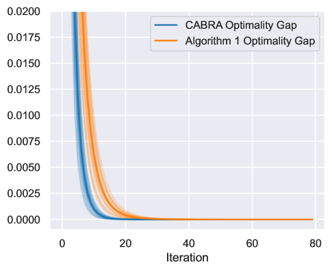
(a) Quadratic optimality gap

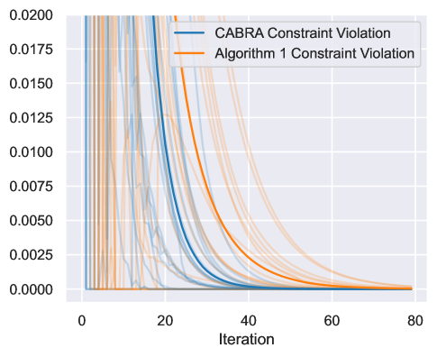
(b) Constraint Violation

Figure 1: Comparison of CABRA and Algorithm 1

5.2 Diagonal Scaling

We now provide a small example of the potential use of these matrix parameters for diagonally scaling the operators. Consider the monotone inclusion

$$\text{find}\;x\in\mathbb{R}^{2}:0\in N_{1}(x)+N_{2}(x)$$ (40)

with

$$c_{1} =(0.05,-1)$$

$$c_{2} =(0.05,1)$$

$$v =(2,2)$$

so that $N_{1}$ and $N_{2}$ are the normal cones of the halfspaces defined by $c_{1}$, $c_{2}$, and $v_{1}$, $v_{2}$. We let $n=2$, $m=0$, $p=2$, and $\mathcal{G}_{k}=\mathbb{R}$. We let $\mathcal{K}^{A}_{1}=\mathcal{K}^{A}_{2}=\mathcal{K}$. Choosing

$$Z_{1}=Z_{2}=W_{1}=W_{2}=\begin{bmatrix}1&-1\\ -1&1\end{bmatrix},$$

initial values $v_{1}^{0}=v_{2}^{0}=(0,0)$, and $\gamma=2$ for Algorithm 3, we get the sequence of iterates $x_{1}^{k}$ and $x_{2}^{k}$ given by Figure 2a. The iterate number is displayed above the points, with the results of resolvent 1 in blue and those of resolvent 2 in orange. Note that, despite $x_{1}^{8}$ and $x_{2}^{8}$ being in the valid region in Figure 2a, the algorithm does not converge until iteration 16, because the subgradient portion of $v_{1}$ and $v_{2}$ has grown in a way that does not sum to zero, and the subgradients have to even out (to zero).

If we instead scale $Z_{1}$ and $W_{1}$ by 0.0025, we get

$$(D_{A})_{1}=(D_{A})_{2}=\begin{bmatrix}0.0025&0\\ 0&1\end{bmatrix}.$$

Using these matrix parameters, we get the sequence of iterates $x_{1}^{k}$ and $x_{2}^{k}$ given by Figure 2b where we converge in two steps rather than 16.

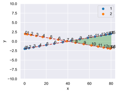
(a) Identical Matrices

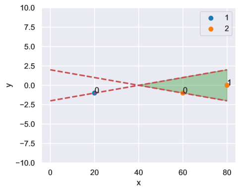
(b) Scaled Matrices

Figure 2: Preconditioning

If we make the halfspace boundaries even more parallel, we can make the convergence of the unscaled matrices arbitrarily slow, while as long as the scaling is sufficiently high, we can achieve two-step convergence with the scaled matrices.

We now apply the same principle to larger problems, including a much larger version of (40), a quadratic problem, and the problem of minimizing the sum of a number of quadratic functions subject to a set of halfspace constraints.

5.2.1 Halfspace Projection

We begin by extending example (40) to $n=30$ and $p=200$, leaving $m=0$ for the time being. As in (40), $\mathcal{K}^{A}_{i}=\mathcal{K}$ for all $i\in\mathcal{I}$ and $\mathcal{G}_{k}=\mathbb{R}$. In each trial, we select halfspaces which are close to parallel by selecting a random vector $c$ uniformly in $[0,2]^{p}$ and then forming the first half of the halfspace normal vectors by adding $c$ to $\left\lfloor\frac{n}{2}\right\rfloor$ random vectors selected uniformly in $[0,.1]^{p}$. We then form the last half of the normal vectors by subtracting $c$ from $n-\left\lfloor\frac{n}{2}\right\rfloor$ random vectors selected uniformly in $[0,.1]^{p}$. We select the constants $v_{i}$ randomly in $[0,1]$. We scale by forming $d_{k}=(c_{ik}^{2})_{i\in\mathcal{I}}$ for each $k\in\mathcal{K}$ and then using the Sinkhorn-Knopp Algorithm [15] as described in [6] to form a symmetric matrix $X_{k}$ with zeros on the diagonal and row and columns sums equal to $d_{k}$. We then let $Z_{k}=W_{k}=\operatorname{diag}(d_{k})-X_{k}$. We compare our scaled matrix parameters with the “uniform" weight matrix parameters given by $Z_{k}=W_{k}=\frac{n}{n-1}\mathrm{Id}-\frac{1}{n-1}\mathbbm{1}\mathbbm{1}^{\intercal}$.

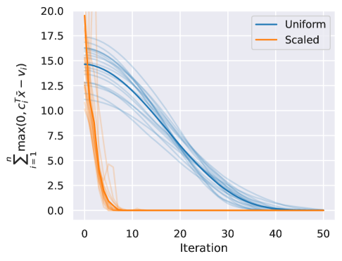
(a) Constraint violation

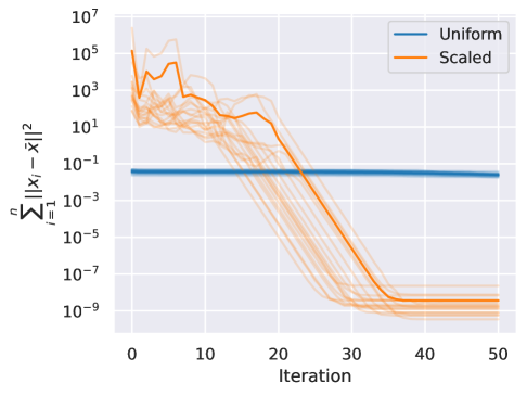
(b) Sum of the squared distances

Figure 3: Diagonal Scaling on Halfspace Projections

Figure 3 shows the results of 20 trials, with the mean for each matrix parameter type in bold and each trial displayed separately in the background. We see that in Figure 3a that the sum of the constraint violation at the mean value $\bar{x}=\frac{1}{n}\sum_{i=1}^{n}x_{i}$ drops much faster for the scaled matrices than the uniform matrices. Figure 3b shows that this comes with a much larger initial sum of the squared distances from the mean, but that once the constraint violation is minimized, this sum of the squared distance quickly approaches zero. If the only concern here is finding a feasible point, the sum of the squared distance from the mean is immaterial and the algorithm can be terminated by taking the first mean value that is feasible.

5.2.2 Quadratic Resolvents

Next, we let $A_{i}(x)=H_{i}x-h_{i}$ for $H_{i}\in\mathbb{S}_{+}^{p}$ and $h_{i}\in\mathbb{R}^{p}$, with $\mathcal{K}^{A}_{i}=\mathcal{K}$ for all $i\in\mathcal{I}$ and $\mathcal{G}_{k}=\mathbb{R}$ as before. In this case, we scale by making $(Z_{k})_{ii}$ similar to $(H_{i})_{kk}+|h_{ik}|$ for each $k\in\mathcal{K}$ and each $i\in\mathcal{I}$. We then let $W_{k}=Z_{k}$. We generate $H_{i}$ by selecting $X_{i}\in\mathbb{R}^{p\times p}$ from a random uniform distribution on $[0,1]^{p\times p}$ and setting $H_{i}=X_{i}^{\intercal}X_{i}$. We generate the data by selecting a central location $c\in\mathbb{R}^{p}$ from a random uniform distribution on $[0,1]^{p}$, and then select a set of random displacement vectors $r_{i}\in\mathbb{R}^{p}$ from a random uniform distribution on $[-.5,.5]^{p}$, forming $h_{i}=c+r_{i}$. We scale via Sinkhorn-Knopp as before.

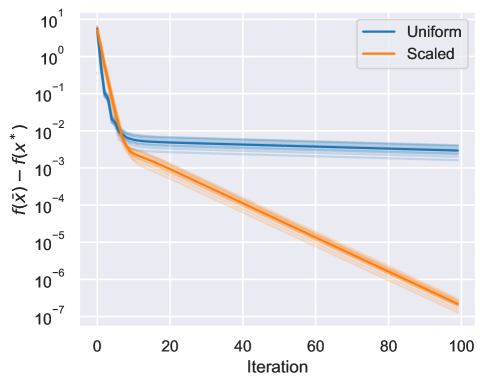
(a) Quadratic optimality gap

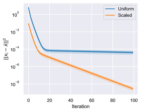
(b) Sum of the squared distances

Figure 4: Diagonal Scaling on Quadratic Operators

Figure 4 shows the results of ten trials with $p=100$, $n=20$, $\alpha=0.5$, and $\gamma=1.75$. We compare the scaled algorithm with the same uniform weight matrices above. We again see much faster convergence and reduction in the sum of the squared distances from the mean.

5.2.3 Halfspace Projection with Quadratic Cocoercive Operators

We now combine the two scenarios, with halfspace projections for each $A_{i}$, so $A_{i}=N_{i}$, and quadratic operators as the cocoercive operators, with $B_{j}(x)=H_{j}x-h_{j}$. We let $\mathcal{K}^{A}_{i}=\mathcal{K}$ and $\mathcal{G}_{k}=\mathbb{R}$ as before. We generate $c_{i}$, $v_{i}$, $H_{j}$, and $h_{j}$ as in 5.2.1 and 5.2.2, but scale each $H_{j}$ so that its maximum eigenvalue is one. We generate the uniform matrices as described in Example 39, which mirrors the most successful approach in [1]. We generate the scaled matrix parameters using (38) with $c=2(1-\cos(\frac{\pi}{n}))$, $s^{k}_{j}=j$ for all $k\in\mathcal{K}$, and $\phi(Z_{k},Q_{k})=\left\lVert d^{Z}_{k}-d^{A}_{k}-Qd^{B}_{k}\right\rVert_{2}+0.1\left\lVert Z_{k}\right\rVert_{2}$ where $d^{Z}_{k}$ is a vector with the diagonal of $Z_{k}$, $d^{A}_{k}=15\alpha(c_{ik}^{2})_{i\in\mathcal{I}}$, and $d^{B}_{k}=\alpha(|h_{jk}|+(H_{j})_{kk})_{j\in\mathcal{J}}$.

Figure 5 shows the results of ten trials with $n=16$, $m=15$, $p=10$, $\alpha=0.25$, and $\gamma=1.85$. The scaled matrices outperform the uniform matrices in convergence to optimality, constraint violation, and convergence of the iterates.

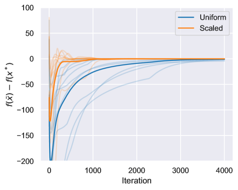
(a) Objective function gap

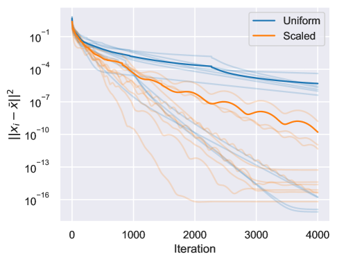
(b) Sum of the squared distances

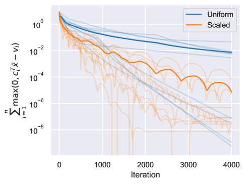
(c) Constraint violation

Figure 5: Diagonal Scaling on Halfspace Projections with Quadratic Operators

5.3 Parallel Execution

Another benefit of (38) as a parameter selection framework is its flexibility in accommodating multi-block parallel execution, which in many cases requires the pattern of $Z$, $W$, and $U$ to be dissimilar. Consider the case where $n=6$, $m=2$, each $R^{A}_{i}$ and $R^{B}_{j}$ is the identity, and we want to use four compute nodes in a distributed manner to calculate the operator values while maximizing parallelization. We can do so by splitting the $A$ operators into three blocks, $(1,2)$, $(3,4)$, and $(5,6)$. We require $Z_{ij}=0$ within each block so that the two members of each block can run without requiring input from one another within the iteration. We also require $W_{ii^{\prime}}=0$ for all $i$ in block 1 and all $i^{\prime}$ in block 3 so that block 1 can begin iteration $\nu+1$ while block 3 finishes iteration $\nu$. We choose $\bar{s}_{t}=2$ and $\text{\@text@baccent{$s$}}_{t}=4$ for all $t\in\mathcal{J}$ so that both cocoercive operators receive input only from block 1 and provide output only to block 3, allowing them to run in parallel with block 2. Assuming all computations require the same amount of time, in steady state we see block 1 and 3 executing in parallel (with block 1 an iteration ahead of block 3), followed by block 2 and the cocoercive operators executing in parallel. In both cases, we use all four computation nodes, ensuring efficient use of available resources, and require no central coordination.

5.4 Stochastic Programming Example

We now consider a multi-stage stochastic version of the relaxed weapon target assignment problem with a finite set of scenarios $\mathcal{S}$, stages $\mathcal{T}$, targets $\mathcal{E}$, and weapons $\mathcal{W}$. The set $\mathcal{X}_{t}$ defines the branches of the scenario tree at stage $t$, and the subset $\mathcal{S}_{bt}\subseteq\mathcal{S}$ defines the scenarios in branch $b$ over which we enforce equality for stage $t$. Let

$$\mathcal{D}=\{(i,j,t,b):(i,j,t)\in\mathcal{W}\times\mathcal{E}\times\mathcal{T},\,b\in\mathcal{X}_{t}\}.$$

We require the following problem parameters and variables:

$$w_{s} \in(0,1)\quad \forall s\in\mathcal{S} \text{probability of scenario}\,s$$

$$V_{j} \in(0,1)\quad \forall j\in\mathcal{E} \text{value of target}\,j$$

$$b_{st} \in\mathcal{X}_{t}\quad \forall s,t\in\mathcal{S}\times\mathcal{T} \text{branch}\,b\text{such that}s\in\mathcal{S}_{bt}$$

$$p_{ijst} \in(0,1)\quad \forall i,j,s,t\in\mathcal{W}\times\mathcal{E}\times\mathcal{S}\times\mathcal{T} \text{damage parameter for target}\,j\,\text{by weapon}\,i$$

$$\text{in scenario}\,s\,\text{and stage}\,t$$

$$x_{ijtb} \in\mathbb{R}\quad \forall i,j,t,b\in\mathcal{D} \text{amount of weapon}\,i\,\text{to use in stage}\,t$$

$$\text{against target}\,j\,\text{ in all scenarios}\,s\in\mathcal{S}_{bt}$$

Let $q_{ijst}=-\log(1-p_{ijst})$. Let $x\in\bigoplus_{(i,j,t)\in\mathcal{W}\times\mathcal{E}\times\mathcal{T}}\mathbb{R}^{|\mathcal{X}_{t}|}$. The problem is then given by

$$\operatorname*{minimize}_{x}\quad \sum_{s\in\mathcal{S}}w_{s}\sum_{j\in\mathcal{E}}V_{j}\exp\left(-\sum_{i\in\mathcal{W}}\sum_{t\in\mathcal{T}}q_{ijst}x_{ijt,b_{st}}\right)$$ (41a)

s.t. $$x_{ijtb}\geq 0\quad\forall i,j,t,b\in\mathcal{D}$$ (41b)

$$\sum_{j\in\mathcal{E}}\sum_{t\in\mathcal{T}}x_{ijt,b_{st}}\leq 1\quad\forall i,s\in\mathcal{W}\times\mathcal{S}.$$ (41c)

Define

$$R^{A}_{is}(x) =(x_{ijt,b_{st}})_{j\in\mathcal{E},t\in\mathcal{T}}\quad \forall i,s\in\mathcal{W}\times\mathcal{S}$$ (42a)

$$R^{B}_{js}(x) =(x_{ijt,b_{st}})_{i\in\mathcal{I},t\in\mathcal{T}}\quad \forall j,s\in\mathcal{E}\times\mathcal{S}$$ (42b)

$$\iota_{0}(x) =\begin{cases}0\quad&\text{if}\;x\geq 0\\ \infty\quad&\text{otherwise}\end{cases}$$ (42c)

$$\iota_{1}(R^{A}_{is}x) =\begin{cases}0\quad&\text{if}\;\sum_{j\in\mathcal{E}}\sum_{t\in\mathcal{T}}x_{ijt,b_{st}}\leq 1\\ \infty\quad&\text{otherwise}\end{cases}$$ (42d)

$$f_{js}(R^{B}_{js}x) =w_{s}V_{j}\exp(-\sum_{i\in\mathcal{W}}\sum_{t\in\mathcal{W}}q_{ijst}x_{ijt,b_{st}})\quad \forall i,s\in\mathcal{W}\times\mathcal{S}.$$ (42e)

Problem (41) can be rewritten as

$$\min_{x}\,\iota_{0}(x)+\sum_{i\in\mathcal{W}}\sum_{s\in\mathcal{S}}\iota_{1}(R^{A}_{is}x)+\sum_{j\in\mathcal{E}}\sum_{s\in\mathcal{S}}f_{js}(R^{B}_{js}x).$$ (43)

We let $N_{0}$ and $N_{1}$ be the normal cones of $\iota_{0}$ and $\iota_{1}$, respectively, and $\nabla f_{js}$ be the derivative of $f_{js}$. Noting that a minimizer exists for (41), both (41) and (43) are equivalent to

$$\text{find}\;x\;\text{s.t.}\;0\in N_{0}(x)+\sum_{i\in\mathcal{W}}\sum_{s\in\mathcal{S}}(R^{A}_{is})^{*}N_{1}(R^{A}_{is}x)+\tau\sum_{j\in\mathcal{E}}\sum_{s\in\mathcal{S}}(R^{B}_{js})^{*}\nabla f_{js}(R^{B}_{js}x).$$ (44)

Note that each element $x_{ijtb}$ of $x$ participates in $N_{0}$ and a total of $|\mathcal{S}_{bt}|$ $N_{1}$ projections, as well as $|\mathcal{S}_{bt}|$ derivatives. Therefore $|\mathcal{I}_{ijtb}|=1+|\mathcal{S}_{bt}|$ and $|\mathcal{J}_{ijtb}|=|\mathcal{S}_{bt}|$.

Since the output of the resolvent on $N_{0}$ is non-negative, we structure the splitting to provide that value as the argument to $\nabla f_{sj}$. On this domain, $\nabla f_{js}$ is $(w_{s}V_{j}\left\lVert q_{js}\right\rVert)^{-1}$-cocoercive. Let $q_{js}=(q_{ijst})_{i,t\in\mathcal{W}\times\mathcal{T}}$ and $\tau=\left(\max_{js}(w_{s}V_{j}\left\lVert q_{js}\right\rVert)\right)^{-1}$, which rescales the problem so that $\beta_{js}\geq 1$ for all derivatives. We can then formulate a parallelizable splitting over the $|W|$ weapons platforms with the following matrix parameters for each element of $x$:

$$Z_{ijtb} \in\mathbb{S}_{+}^{1+|\mathcal{S}_{bt}|} Z_{ijtb}=\begin{bmatrix}|S_{bt}|&-\mathbbm{1}^{\intercal}\\ -\mathbbm{1}&\mathrm{Id}\end{bmatrix}$$ (45a)

$$W_{ijtb} \in\mathbb{S}_{+}^{1+|\mathcal{S}_{bt}|} W_{ijtb}=\mathrm{Id}-\frac{1}{1+|\mathcal{S}_{bt}|}\mathbbm{1}\mathbbm{1}^{\intercal}$$ (45b)

$$K_{ijtb} \in\mathbb{R}^{|\mathcal{S}_{bt}|\times(1+|\mathcal{S}_{bt}|)} K_{ijtb}=\begin{bmatrix}\mathbbm{1}&\mathbf{0}\mathbf{0}^{\intercal}\end{bmatrix}$$ (45c)

$$Q_{ijtb} \in\mathbb{R}^{(1+|\mathcal{S}_{bt}|)\times|\mathcal{S}_{bt}|} Q_{ijtb}=\begin{bmatrix}\mathbf{0}^{\intercal}\\ \frac{1}{|\mathcal{S}_{bt}|}\mathbbm{1}\mathbbm{1}^{\intercal}\end{bmatrix}$$ (45d)

$$U_{ijtb} \in\mathbb{S}_{+}^{1+|\mathcal{S}_{bt}|} U_{ijtb}=\begin{bmatrix}|S_{bt}|&-\mathbbm{1}^{\intercal}\\ -\mathbbm{1}&\frac{1}{|\mathcal{S}_{bt}|}\mathbbm{1}\mathbbm{1}^{\intercal}\end{bmatrix}.$$ (45e)

These matrices satisfy (6). Using them, we can find the resolvent of $N_{0}$ in parallel over the $|\mathcal{W}|$ platforms (by the separability of $N_{0}$). Each platform $i$ can then find $\sum_{t\in\mathcal{T}}q_{ijst}x_{ijt,b_{st}}$ for all $j,s$, and provide it to the other platforms. Upon receiving the corresponding transmission from the other platforms, each platform can calculate $f_{js}$ for all $j,s$, and then compute the $s$ resolvents of $N_{1}(R^{A}_{is}x)$ by providing $\frac{-1}{|\mathcal{S}_{bt}|}\sum_{s\in\mathcal{S}_{bt}}q_{ijst}f_{js}$ as the $(Q_{A}BK_{A})_{ijtb}$ portion of the resolvent argument. Each platform can then update $\mathbf{v}_{ijtb}$ independently for all $j$, $t$, and $b$, and proceed to the next iteration. In this formulation, only one communication is required between platforms in each iteration, and that communication is reduced to only $|\mathcal{E}\times\mathcal{S}|$ scalars, and can be even smaller if some platforms have $q_{ijst}=0$ for some $j$ and $s$.

6 Conclusion

This research extends the matrix-parametrized frugal resolvent splitting framework with minimal lifting to include the composition of maximal monotone and cocoercive operators with arbitrary selection operators. It also offers a framework for selecting valid matrix parameters, and demonstrates its use for parallelization and potential for preconditioning. We present an application of the new algorithm to decentralized stochastic programming. We show that CABRA generalizes Algorithm 1, and outperforms Algorithm 1 experimentally in a case where the selection operators are not the identity.

The CABRA algorithm, and the matrix parameter selection framework, offer a number of promising directions for future research. Extending it to include arbitrary linear compositions appears particularly promising. We also believe research into optimal preconditioning matrices will prove fruitful, particularly in the space of trade-offs between preconditioning and efficient parallel execution.

Acknowledgements Both authors acknowledge support from Office of Naval Research awards N0001425WX00069 and N0001425GI01512.

Appendix A Appendix

A.1 Supporting Lemmas

Lemma 4.

The permuted operator $\mathbf{P}_{A}\mathbf{L}\mathbf{P}_{A}^{*}$ is strictly block lower triangular.

Proof.

By definition, $L_{k}$ is strictly lower triangular for each $k$. Therefore if $(L_{k})_{rc}$ is non-zero, $r>c$, and $r$ and $c$ correspond with operator indices $i_{r}$ and $i_{c}$ such that $r=s(i_{r},k)$ and $c=s(i_{c},k)$ and $i_{r}>i_{c}$ since $s(i,k)$ gives the order of $i$ in the ordered set $\mathcal{I}_{k}$. Let $o(i,k)$ give the order of entry $k$ in $\mathcal{K}^{A}_{i}$ and $\delta_{i}=\sum_{d=1}^{i-1}|\mathcal{K}^{A}_{d}|$. Given $\mathbf{y}\in\mathcal{H}_{\text{y}}$, the permutation operator $\mathbf{P}_{A}$ permutes $\mathbf{y}_{k,s(i,k)}$ to the position in $x\in\mathcal{H}_{\text{x}}$ given by $\text{ind}(i,k)=\delta_{i}+o(i,k)$. Therefore, in $\mathbf{P}_{A}\mathbf{L}\mathbf{P}_{A}^{*}$, the only non-zero entries correspond with the permuted locations of $i_{r}$ and $i_{c}$ given by row $\text{ind}(i_{r},k)$ and column $\text{ind}(i_{c},k)$ for all $k$. Since $i_{c}<i_{r}$, we have $\text{ind}(i_{c},k)=\delta_{i_{c}}+o(i_{c},k)\leq\delta_{i_{c}}+|\mathcal{K}^{A}_{i_{c}}|<\delta_{i_{r}}+1\leq\delta_{i_{r}}+o(i_{r},k)=\text{ind}(i_{r},k)$. Therefore, with block cutoffs in $\mathbf{L}_{A}$ defined by $d_{i}$, $\mathbf{P}_{A}\mathbf{L}\mathbf{P}_{A}^{*}$ is strictly block lower triangular. ∎

Lemma 5.

Operator $\mathbf{Q}_{A}\mathbf{B}\mathbf{K}_{A}$ is strictly lower triangular in the sense that $\left(\mathbf{Q}_{A}\mathbf{B}\mathbf{K}_{A}\mathbf{x}\right)_{i}$ depends only on subvectors $x_{d}$ of $\mathbf{x}$ such that $d<i$.

Proof.

By definition $\mathbf{Q}_{A}\mathbf{B}\mathbf{K}_{A}=\mathbf{P}_{A}\mathbf{Q}\mathbf{P}_{B}^{*}\mathbf{B}\mathbf{P}_{B}\mathbf{K}\mathbf{P}_{A}^{*}$. By (6k) and (13), the maximum operator index $i_{k}$ which feeds the output associated with $B_{j}$ in $K_{k}$ for $k\in\mathcal{K}^{B}_{j}$ must be less than or equal to $i^{*}_{j}$ for all $k$. By definition, permutation operator $\mathbf{P}_{A}^{*}$ preserves operator ordering as it groups the ordered input for each $K_{k}$, and permutation operator $\mathbf{P}_{B}$ preserves operator ordering as it groups the outputs which feed cocoercive operator $B_{j}$ from each $K_{k}$ where $k\in\mathcal{K}^{B}_{j}$. Therefore $(\mathbf{P}_{B}\mathbf{K}\mathbf{P}_{A}^{*})_{j}$ depends only on operators $A_{i}$ for $i\leq i^{*}_{j}$ (that is, $(\mathbf{P}_{B}\mathbf{K}\mathbf{P}_{A}^{*})_{ji}=0$ for all $i>i^{*}_{j}$). Equations (6k) and (13) also require that $\bar{s}^{k}_{j}<\text{\@text@baccent{$s$}}_{t(j,k)}$ for all $k$ and for all $j\in\mathcal{J}_{k}$, so $Q_{k}$ equals zero for all entries associated with operators $A_{i}$ and $B_{j}$ where $i\leq i^{*}_{j}$. This means that $(\mathbf{P}_{A}\mathbf{Q}\mathbf{P}_{B}^{*})_{ij}=0$ for all $i\leq i^{*}_{j}$. Therefore $B_{j}(\mathbf{P}_{B}\mathbf{K}\mathbf{P}_{A}^{*})_{j}$ is not required by all operators $A_{i}$ where $i\leq i^{*}_{j}$, and for $i>i^{*}_{j}$, $B_{j}(\mathbf{P}_{B}\mathbf{K}\mathbf{P}_{A}^{*})_{j}$ depends only on outputs from $A_{i^{\prime}}$ where $i^{\prime}\leq i^{*}_{j}<i$, and can be found prior to the computation of $A_{i}$.

∎

Lemma 6.

The set $\mathcal{N}_{A}$ is the null space of $\mathbf{M}_{A}$, $\mathbf{W}_{A}$, and $\mathbf{Z}_{A}$.

Proof.

For any $\mathbf{x}\in\mathcal{N}_{A}$, we know that $\mathbf{P}_{A}^{*}\mathbf{x}=\left(\mathbbm{1}\otimes y_{k}\right)_{k\in\mathcal{K}}$ for subvectors $y_{k}\in\mathcal{G}_{k}$. This follows from the construction of $\mathbf{P}_{A}$ and the definition of $\mathcal{N}_{A}$. By the requirements of (6) on $M_{k}$, $W_{k}$, and $Z_{k}$,

$$M_{k}\mathbbm{1}=W_{k}\mathbbm{1}=Z_{k}\mathbbm{1}=0.$$

Therefore for $y\in\bigoplus_{k\in\mathcal{K}}\mathcal{G}_{k}$ and $\mathbf{x}=\mathbf{R}_{A}y\in\mathcal{N}_{A}$, and $\mathbf{y}_{\mathbbm{1}}=\mathbf{P}_{A}^{*}\mathbf{x}=(\mathbbm{1}\otimes y_{k})_{k\in\mathcal{K}}$,

$$\mathbf{W}_{A}\mathbf{x}=\mathbf{P}_{A}\mathbf{W}\mathbf{P}_{A}^{*}\mathbf{x}=\mathbf{P}_{A}\left(W_{k}\mathbbm{1}\otimes y_{k}\right)_{k\in\mathcal{K}} =0$$

$$\mathbf{Z}_{A}\mathbf{x}=\mathbf{P}_{A}\mathbf{Z}\mathbf{P}_{A}^{*}\mathbf{x}=\mathbf{P}_{A}\left(Z_{k}\mathbbm{1}\otimes y_{k}\right)_{k\in\mathcal{K}} =0$$

$$\mathbf{M}_{A}\mathbf{x}=\mathbf{P}_{A}\mathbf{M}\mathbf{P}_{A}^{*}\mathbf{x}=\mathbf{P}_{A}\left(M_{k}\mathbbm{1}\otimes y_{k}\right)_{k\in\mathcal{K}} =0$$

We therefore have

$$\mathcal{N}_{A} \subseteq\operatorname{null}{M}_{A}$$

$$\mathcal{N}_{A} \subseteq\operatorname{null}{W}_{A}$$

$$\mathcal{N}_{A} \subseteq\operatorname{null}{Z}_{A}.$$

Since $\operatorname{null}(W_{k})=\text{span}(\mathbbm{1})$, $W_{k}=M_{k}^{\intercal}M_{k}$, $Z\succeq W$, and $Z\mathbbm{1}=0$, we have

$$\operatorname{null}{(M_{k})} =\text{span}(\mathbbm{1})$$

$$\operatorname{null}{(Z_{k})} =\text{span}(\mathbbm{1})$$

and for any $\mathbf{y}_{k}\in\mathcal{G}_{k}^{n_{k}}$ such that $\mathbf{y}_{k}\neq\mathbbm{1}\otimes y_{k}$ for some $y_{k}\in\mathcal{G}_{k}$, $\mathbf{y}_{k}$ is not in the null space of $M_{k}$, $W_{k}$, or $Z_{k}$.

For any $\mathbf{x}\notin\mathcal{N}_{A}$, at least one set of coupling constraints is not satisfied. Let $\mathbf{y}=\mathbf{P}_{A}^{*}\mathbf{x}$, and $\mathbf{y}_{k}\in\mathcal{G}_{k}^{n_{k}}$ be a subvector of $\mathbf{y}$ which does not satisfy the coupling constraint, and therefore is not in the span of the ones vector. Then

$$\mathbf{M}_{k}\mathbf{y}_{k} \neq 0$$

$$\mathbf{W}_{k}\mathbf{y}_{k} \neq 0$$

$$\mathbf{Z}_{k}\mathbf{y}_{k} \neq 0$$

Therefore

$$\operatorname{null}{\mathbf{M}_{A}}=\operatorname{null}{\mathbf{W}_{A}}=\operatorname{null}{\mathbf{Z}_{A}}=\mathcal{N}_{A}.$$

∎

A direct corollary of Lemma 6 is the fact that

$$\operatorname{ran}(\mathbf{M}^{*}_{A})=\mathcal{N}_{A}^{\perp}.$$ (46)

For $\mathbf{x}\in\mathcal{N}_{A}$, there is a similar correspondence between $\mathbf{P}_{A}^{*}(\mathbf{D}-2\mathbf{L})\mathbf{P}_{A}\mathbf{x}$ and $\mathcal{N}_{A}^{\perp}$, which we establish in Lemma 7.

Lemma 7.

If $\mathbf{x}\in\mathcal{N}_{A}$ then $(\mathbf{D}_{A}-2\mathbf{L}_{A})\mathbf{x}\in\mathcal{N}_{A}^{\perp}$.

Proof.

Let $\mathbf{x}^{\perp}\in\mathcal{N}_{A}^{\perp}$ and $\mathbf{x}\in\mathcal{N}_{A}$. We have already established by definition that

$$\left\langle\mathbf{x}^{\perp},\mathbf{x}\right\rangle =0$$

$$\left\langle\mathbf{P}_{A}\mathbf{x}^{\perp},\mathbf{P}_{A}\mathbf{x}\right\rangle =0$$

$$\mathbf{P}_{A}\mathbf{x} =\left(\mathbbm{1}\otimes y_{k}\right)_{k\in\mathcal{K}}$$

for some subvectors $y_{k}\in\mathcal{G}_{k}$. We therefore know that

$$(\mathbf{D}-2\mathbf{L})\mathbf{P}_{A}\mathbf{x}=\left((D_{k}-2L_{k})\mathbbm{1}\otimes y_{k}\right)_{k\in\mathcal{K}}.$$

By assumption (6c), we know that each $Z_{k}$ is symmetric and $Z_{k}\mathbbm{1}=0$, so $\mathbbm{1}^{\intercal}Z_{k}\mathbbm{1}=0$. We also know by assumption (7a) that $Z_{k}=D_{k}-L_{k}-L_{k}^{\intercal}$, so $\mathbbm{1}^{\intercal}(D_{k}-2L_{k})\mathbbm{1}=\mathbbm{1}^{\intercal}Z_{k}\mathbbm{1}=0$. This means that for each $k$, $\left\langle\mathbbm{1}\otimes y^{1}_{k},(\mathbf{D}_{k}-2\mathbf{L}_{k})(\mathbbm{1}\otimes y_{k})\right\rangle=0$. For any $\mathbf{x}^{1}\in\mathcal{N}_{A}$ and $\mathbf{y}^{1}=\mathbf{P}_{A}\mathbf{x}^{1}=\left(\mathbbm{1}\otimes y_{k}^{1}\right)_{k\in\mathcal{K}}$, we then have

$$\left\langle\mathbf{x}^{1},\mathbf{P}_{A}^{*}(\mathbf{D}-2\mathbf{L})\mathbf{P}_{A}\mathbf{x}\right\rangle =\left\langle\mathbf{P}_{A}\mathbf{x}^{1},(\mathbf{D}-2\mathbf{L})\mathbf{P}_{A}\mathbf{x}\right\rangle$$

$$=\sum_{k=1}^{p}\left\langle\mathbbm{1}\otimes y_{k}^{1},(D_{k}-2L_{k})(\mathbbm{1}\otimes y_{k})\right\rangle$$

$$=0$$

Therefore

$$\mathbf{P}_{A}^{*}(\mathbf{D}-2\mathbf{L})\mathbf{P}_{A}\mathbf{x}\in\mathcal{N}_{A}^{\perp}\quad\forall\mathbf{x}\in\mathcal{N}_{A}$$ (47)

∎

Lemma 8.

For any sequence $(\mathbf{z}^{k})$ given by $\mathbf{z}^{k+1}=T(\mathbf{z}^{k})$, its corresponding sequence $(\mathbf{x}^{k})$ given by (4) is also bounded.

Proof.

This can be shown by induction over the sequences $(x_{i}^{k})$ of $(\mathbf{x}^{k})$. Beginning with $i=1$, we have by the nonexpansivity of the resolvent

$$\left\lVert x_{1}^{k}\right\rVert =\left\lVert J_{\alpha(\mathbf{D}_{A}^{-1})_{1}A_{1}}\left(-(\mathbf{D}_{A}^{-1})_{1}(\mathbf{M}^{*}_{A}\mathbf{z}^{k})_{1}\right)\right\rVert$$

$$\leq\left\lVert(\mathbf{D}_{A}^{-1})_{1}(\mathbf{M}^{*}_{A}\mathbf{z}^{k})_{1}\right\rVert$$

which is bounded by the boundedness of $(\mathbf{z}^{k})$, $\mathbf{D}_{A}^{-1}$, and $\mathbf{M}_{A}$.

Suppose $(x_{d}^{k})$ is bounded for $d<i$. We now show that $(x_{i}^{k})$ is bounded. By Lemmas 4 and 5, $(\mathbf{L}_{A}\mathbf{x})_{i}$ and $(\mathbf{Q}_{A}\mathbf{B}\mathbf{K}_{A}\mathbf{x})_{i}$ depend only on values $x_{d}^{k}$ for $d<i$. Therefore $(\mathbf{L}_{A}\mathbf{x}^{k})_{i}$ and $(\mathbf{K}_{A}\mathbf{x}^{k})_{j}$ for all $Q_{ij}\neq 0$ are bounded by the induction hypothesis and the boundedness of $\mathbf{L}_{A}$ and $\mathbf{K}_{A}$, and $(\mathbf{Q}_{A}\mathbf{B}\mathbf{K}_{A}\mathbf{x}^{k})_{i}$ is bounded by the boundedness of $\mathbf{Q}_{A}$ and the cocoercivity of $\mathbf{B}$. The boundedness of $(\mathbf{z}^{k})$ implies the boundedness of $(\mathbf{M}^{*}_{A}\mathbf{z}^{k})_{i}$, and we therefore see that

$$\left\lVert x_{i}^{k}\right\rVert =\left\lVert J_{\alpha(\mathbf{D}_{A}^{-1})_{i}A_{i}}\left((\mathbf{D}_{A}^{-1})_{i}\left[-(\mathbf{M}^{*}_{A}\mathbf{z}^{k})_{i}-\alpha(\mathbf{Q}_{A}\mathbf{B}\mathbf{K}_{A}\mathbf{x}^{k})_{i}+(2\mathbf{L}_{A}\mathbf{x}^{k})_{i}\right\rVert\right]\right)$$

$$\leq\left\lVert(\mathbf{D}_{A}^{-1})_{i}(\mathbf{M}^{*}_{A}\mathbf{z}^{k})_{i}\right\rVert+\alpha\left\lVert(\mathbf{D}_{A}^{-1})_{i}(\mathbf{Q}_{A}\mathbf{B}\mathbf{K}_{A}\mathbf{x}^{k})_{i}\right\rVert+\left\lVert(\mathbf{D}_{A}^{-1})_{i}(2\mathbf{L}_{A}\mathbf{x}^{k})_{i}\right\rVert$$

is bounded for all $k$. Therefore, by induction, $(\mathbf{x}_{i}^{k})$ is bounded for all $i\in\mathcal{I}$, and $(\mathbf{x}^{k})$ is bounded. ∎

A.2 Decentralized Algorithm

Algorithm 4 Decentralized Expanded CABRA

1:$\alpha\in(0,4)$; $\gamma_{\nu}\in(0,2-\frac{\alpha}{2})$; $\mathbf{v}^{0}\in\mathcal{N}^{\perp}$; $\mathbf{D}_{A}^{-1}$, $\mathbf{W}_{A}$, $\mathbf{L}_{A}$, $\mathbf{Q}_{A}$, $\mathbf{K}_{A}$ satisfying (21).

2:$\nu\leftarrow 0$

3:repeat

4:  for $i=1,\dots,n$ in parallel do

5:   for $d=1,\dots,i-1$ do

6:     for $k\in\mathcal{K}^{A}_{d}\bigcap\mathcal{K}^{A}_{i}:(L_{k})_{id}\neq 0$ or $(W_{k})_{id}\neq 0$ do

7:      Receive $(x_{d})^{\nu}_{k}$ from maximal monotone operator $d$

8:     end for

9:     for $j=1,\dots,m:i^{*}_{j}=d$ do

10:      for $k\in\mathcal{K}^{B}_{j}\bigcap\mathcal{K}^{A}_{i}:(Q_{k})_{ij}\neq 0$ do

11:        Receive $(b_{j})^{\nu}_{k}$ from cocoercive operator $j$

12:      end for

13:     end for

14:   end for

15:   $\mathbf{x}_{i}^{\nu}=J_{\alpha(\mathbf{D}_{A}^{-1}\mathbf{A})_{i}}\left((\mathbf{D}_{A}^{-1})_{i}\left[\mathbf{v}_{i}^{\nu}+2(\mathbf{L}_{A}\mathbf{x}^{\nu})_{i}-\alpha(\mathbf{Q}_{A}\mathbf{b}^{\nu})_{i}\right]\right)$

16:   for $k\in\mathcal{K}^{A}_{i}$ do

17:     for $d=i+1,\dots,n:k\in\mathcal{K}^{A}_{d}$ do

18:      if $(L_{k})_{di}\neq 0$ or $W_{di}\neq 0$ then

19:        Send $(x_{i})^{\nu}_{k}$ to maximal monotone operator $d$

20:      end if

21:     end for

22:     for $j=1,\dots,m:k\in\mathcal{K}^{B}_{j}$ and $(\mathbf{K}_{k})_{ji}\neq 0$ do

23:      Send $(x_{i})^{\nu}_{k}$ to cocoercive operator $j$

24:     end for

25:     for $d=1,\dots,i-1:k\in\mathcal{K}^{A}_{d}\bigcap\mathcal{K}^{A}_{i}$ and $W_{id}\neq 0$ do

26:      Send $(x_{i})^{\nu}_{k}$ to maximal monotone operator $d$

27:     end for

28:     for $d=i+1,\dots,n$ do

29:      if $k\in\mathcal{K}^{A}_{d}$ and $W_{id}\neq 0$ then

30:        Receive $(x_{d})^{\nu}_{k}$ from maximal monotone operator $d$

31:      end if

32:     end for

33:   end for

34:   $\mathbf{v}_{i}^{\nu+1}=\mathbf{v}_{i}^{\nu}-\gamma_{\nu}(\mathbf{W}_{A}\mathbf{x}^{\nu})_{i}$

35:  end for

36:  for $j=1,\dots,m$ in parallel with above do

37:   for $i=1,\dots,i^{*}_{j}$ do

38:     for $k\in\mathcal{K}^{B}_{j}\bigcap\mathcal{K}^{A}_{i}:(K_{k})_{ji}\neq 0$ do

39:      Receive $(x_{i})^{\nu}_{k}$ from maximal monotone operator $i$

40:     end for

41:   end for

42:   $\mathbf{b}_{j}^{\nu}=\alpha\mathbf{B}_{j}(\mathbf{K}_{A}\mathbf{x}^{\nu})_{j}$

43:   for $i=i^{*}_{j}+1,\dots,n$ do

44:     for $k\in\mathcal{K}^{B}_{j}\bigcap\mathcal{K}^{A}_{i}:(Q_{k})_{ij}\neq 0$ do

45:      Send $(b_{j})^{\nu}_{k}$ to maximal monotone operator $i$

46:     end for

47:   end for

48:  end for

49:  $\nu\leftarrow\nu+1$

50:until convergence

References

- \bibcommenthead
- Åkerman et al [2025] Åkerman A, Chenchene E, Giselsson P, et al (2025) Splitting the forward-backward algorithm: A full characterization. arXiv preprint arXiv:250410999 URL https://arxiv.org/abs/2504.10999
- ApS [2024] ApS M (2024) MOSEK Optimizer API for Python 10.2.1. URL https://docs.mosek.com/latest/pythonapi/index.html
- Aragón-Artacho et al [2023a] Aragón-Artacho FJ, Boţ RI, Torregrosa-Belén D (2023a) A primal-dual splitting algorithm for composite monotone inclusions with minimal lifting. Numerical Algorithms 93(1):103–130
- Aragón-Artacho et al [2023b] Aragón-Artacho FJ, Malitsky Y, Tam MK, et al (2023b) Distributed forward-backward methods for ring networks. Computational Optimization and Applications 86(3):845–870
- Aragón-Artacho et al [2024] Aragón-Artacho FJ, Campoy R, López-Pastor C (2024) Forward-backward algorithms devised by graphs. arXiv preprint arXiv:240603309
- Barkley and Bassett [2025] Barkley P, Bassett RL (2025) Decentralized sensor network localization using matrix-parametrized proximal splittings. URL https://arxiv.org/abs/2503.13403, 2503.13403
- Bassett and Barkley [2024] Bassett RL, Barkley P (2024) Optimal design of resolvent splitting algorithms. URL https://arxiv.org/abs/2407.16159, 2407.16159
- Bauschke et al [2011] Bauschke HH, Combettes PL, et al (2011) Convex analysis and monotone operator theory in Hilbert spaces, vol 408. Springer
- Bredies et al [2022] Bredies K, Chenchene E, Lorenz DA, et al (2022) Degenerate preconditioned proximal point algorithms. SIAM Journal on Optimization 32(3):2376–2401
- Bredies et al [2024] Bredies K, Chenchene E, Naldi E (2024) Graph and distributed extensions of the Douglas–Rachford method. SIAM Journal on Optimization 34(2):1569–1594
- Dao et al [2025] Dao MN, Tam MK, Truong TD (2025) A general approach to distributed operator splitting. arXiv preprint arXiv:250414987
- Malitsky and Tam [2023] Malitsky Y, Tam MK (2023) Resolvent splitting for sums of monotone operators with minimal lifting. Mathematical Programming 201(1-2):231–262
- Morin et al [2024] Morin M, Banert S, Giselsson P (2024) Frugal splitting operators: Representation, minimal lifting, and convergence. SIAM Journal on Optimization 34(2):1595–1621. 10.1137/22M1531105
- Ryu [2020] Ryu EK (2020) Uniqueness of DRS as the 2 operator resolvent-splitting and impossibility of 3 operator resolvent-splitting. Mathematical Programming 182(1-2):233–273
- Sinkhorn and Knopp [1967] Sinkhorn R, Knopp P (1967) Concerning nonnegative matrices and doubly stochastic matrices. Pacific Journal of Mathematics 21(2):343–348
- Stewart [1980] Stewart GW (1980) The efficient generation of random orthogonal matrices with an application to condition estimators. SIAM Journal on Numerical Analysis 17(3):403–409
- Tam [2023] Tam MK (2023) Frugal and decentralised resolvent splittings defined by nonexpansive operators. Optimization Letters pp 1–19