Stabilized velocity post-processings for Darcy flow in heterogeneous porous media

Abstract.

Stable and accurate finite element methods are presented for Darcy flow in heterogeneous porous media with an interface of discontinuity of the hydraulic conductivity tensor. Accurate velocity fields are computed through global or local post-processing formulations that use previous approximations of the hydraulic potential. Stability is provided by combining Galerkin and Least Squares (GLS) residuals of the governing equations with an additional stabilization on the interface that incorporates the discontinuity on the tangential component of the velocity field in a strong sense. Numerical analysis is outlined and numerical results are presented to illustrate the good performance of the proposed methods. Convergence studies for a heterogeneous and anisotropic porous medium confirm the same orders of convergence predicted for homogeneous problem with smooth solutions, for both global and local post-processings.

Keywords

Stabilized Finite Element, Global Post-Processing, Local Post-Processing, Galerkin Least Squares, Heterogeneous Porous Media

1. Introduction

Transport problems associated with reservoir simulation, groundwater contamination or remediation demands information about the macroscopic (average) velocity of the phases flowing in the porous formation. These flows are, in general, highly advective and accurate approximations of the velocity fields are crucial for the evaluation of the related transport processes.

The system of partial differential equations that models the flow of an incompressible homogeneous fluid in a rigid saturated porous media consists basically of the mass conservation equation plus Darcy’s law, relating the average velocity of the fluid with the gradient of a potential field through the hydraulic conductivity tensor. A standard way to solve this system is based on the second order elliptic equation obtained by substituting Darcy’s law in the mass conservation equation leading to a Poisson problem in the potential field with velocity calculated by taking the gradient of the solution multiplied by the hydraulic conductivity. Constructing finite element methods based on this kind of formulation is straightforward. However, this direct approach leads to lower-order approximations for velocity compared to potential and, additionally, the corresponding balance equation is enforced in an extremely weak sense. Alternative formulations have been employed to enhance the velocity approximation like post-processing techniques and mixed methods.

The basic idea of the post-processing formulations is to use the optimal stability and convergence properties of the classical Galerkin approximation for the potential field to derive more accurate velocity approximations than that obtained by direct application of Darcy’s law. In [10] a post-processed continuous flux (normal component of the velocity) distribution over the porous media domain is derived using patches with flux-conserving boundaries. Another conservative post-processing based on a control volume finite element formulation is presented in [12]. Within the context of adaptive analysis, a local post-processing, is introduced in [9], named Superconvergent Patch Recovery, to recover higher order approximations for the gradients of finite element solutions.

Mixed methods are based on the simultaneous approximation of potential and velocity fields, and their main characteristic is the use of different spaces for velocity and potential to satisfy a compatibility between the finite element spaces, which reduces the flexibility in constructing finite approximations (LBB condition - [1, 8]). A well known successful approach is the dual mixed formulation developed by Raviart and Thomas [2] using divergence based finite element spaces for the velocity field combined with discontinuous Lagrangian spaces for the potential. Stabilized mixed finite element methods have been proposed to overcome the compatibilty conditions between the finite element spaces, see [19, 6, 17] and references therein. In general, stabilized formulations use Lagrangian finite element spaces and have been successfully employed in simulating Darcy’s flows in homogeneous porous media. The point is their applicability to problems where the porous formation is composed by subdomains with different conductivities. On the interface between these subdomains, the normal component of Darcy velocity must be continuous (mass conservation) but the tangential component is discontinuous, and any formulation based on $C^{0}$ Lagrangian interpolation for velocity fails in representing the tangential discontinuity, producing inaccurate approximations and spurious oscillations, while completely discontinuous approximations for velocity do not necessarily fit the continuity of the flux. Interesting alternatives are the discontinuous Galerkin methods [19, 21], or coupling continuous and discontinuous Galerkin methods as in [20].

In this work we will be concened with post-processing techniques derived form variational formulations with good stability and convergence properties on Lagrangian finite element spaces. In particular, we consider those based on stabilized finite element methods, such as the global $C^{0}$ post-processing derived in [7] by adding a least-square residual of the mass conservation to a weak form of Darcy’s law, and the local post-processing (by element or macroelement) introduced in [14] which combines least squares residuals of both conservation of mass and irrotationality condition with a discrete least squares residual of Darcy’s law taken at the superconvergence points of the gradient of the potential. These formulations give velocity approximations with higher convergence orders than those obtained by the simple direct use of Darcy’s law. One important feature of the global post-processing approach is the flexibility in the choice of finite element spaces, allowing the use of equal-order Lagrangian spaces, for example. In [16] miscible displacement analyses are performed using $C^{0}$ Lagrangian interpolations of the same order for potential, velocity and concentration.

Here we study the approximation of flows in porous media composed by layers with different conductivities, using Lagrangian-based stabilized finite element methods. We show that the Global Post-Processing presented in [7, 14] can be derived from a Galerkin Least-Squares stabilized mixed formulation and popose generalized versions of the global and local post-processing in which equal-order Lagrangian finite element spaces are naturally adopted to porous media with interfaces of discontinuity of the hydraulic conductivity. For smooth interfaces of discontinuity, the proposed generalization of the global $C^{0}$ post-processing preserves the continuity of the flux and exactly imposes the constraint between the tangent components of Darcy velocity on the interface of the layers. By construction, the local post-processing naturally accommodates discontinuities of the tangent component but it does not ensure continuity of the normal component of the velocity field on the macroelement interfaces. When the interface of discontinuity is put in the interior of a macroelement, the continuity or discontinuity constraints on the normal and tangential components of Darcy’s velocity are exactly imposed.

After introducing some notations and definitions in Section 2, we present in Section 3 our model problem for the flow in a porous media with a smooth interface of discontinuity of the hydraulic conductivity, consisting in a system of partial differential equation with appropriate boundary and interface conditions. The standard Galerkin finite element method is reviewed in Section 4. Stabilized mixed finite element methods are briefly discussed in Section 5. In Section 6 we associate the origin of the considered post-processing techniques with stabilized mixed formulations and propose a generalization of global and local post-processings to porous media with interface of discontinuity. Numerical experiments illustrating the performance of the global and local post-processing are reported in Section 7 and in Section 8 we draw some conclusions.

2. Notations and Definitions

Given $\Omega$ a bounded subdomain of $\mathbb{R}^{2}$, with a sufficiently smooth boundary $\partial\Omega$, let $L^{2}(\Omega)$ be the space of square integrable functions in $\Omega$. For $m\geq 0$ integer, we define $H^{m}(\Omega)$ the Hilbert space over $\Omega$ of order $m$

$$H^{m}=\{v\in L^{2}(\Omega);D^{\alpha}v\in L^{2}(\Omega),|\alpha|\leq m\}\mbox{, where}$$

$$D^{\alpha}(\cdot):=\frac{\partial^{|\alpha|}(\cdot)}{\partial_{x_{1}}^{\alpha_{1}}\partial_{x_{2}}^{\alpha_{2}}},\quad|\alpha|=\alpha_{1}+\alpha_{2},\;\mbox{ and }\;\alpha=(\alpha_{1},\alpha_{2})\mbox{ is an array}\in\mathbb{N}^{2}.$$

The inner product and the norm in $H^{m}(\Omega)$ are given by

$$(v,w)_{m}:=\sum_{|\alpha|\leq m}\int_{\Omega}D^{\alpha}v\,D^{\alpha}w\operatorname{d\Omega},\quad\|v\|_{m}=(v,v)_{m}^{1/2}.$$

We denote $H^{1}_{0}(\Omega)=\{v\in H^{1}(\Omega);\left.v\right|_{\partial\Omega}=0\}$ and define the space

$${H(\operatorname{div})}=\left\{\bm{u}\in\left(L^{2}(\Omega)\right)^{2};\;\operatorname{\mathrm{div}}\bm{u}\in L^{2}(\Omega)\right\},\mbox{ with norm }$$

$$\|\bm{u}\|_{H(\operatorname{div})}:=\left\{\|\bm{u}\|^{2}+\|\operatorname{\mathrm{div}}\bm{u}\|^{2}\right\}^{1/2}.$$

Finally, $H^{0}(\Omega)=L^{2}(\Omega)$ has norm $\|\cdot\|_{0}=\|\cdot\|$ and inner product given by

$$(v,w):=\int_{\Omega}v\,w\operatorname{d\Omega}.$$

3. Model Problem

Let $\Omega=\Omega_{1}\cup\Omega_{2}\subset\mathbb{R}^{2}$, with smooth boundary $\partial\Omega$ and outward unit normal vector $\bm{n}$, be the domain of a rigid porous media saturated with an incompressible homogeneous fluid. The domain $\Omega$ is composed by two subdomains $\Omega_{1}$ and $\Omega_{2}$ that represent regions with different conductivities, jointed by a smooth interface $\Gamma$, as illustrated in Fig 1.

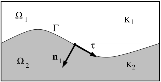
Figure 1. Domain of the model problem.

The mass balance asserts that

$$\operatorname{\mathrm{div}}\bm{u}=f\quad\mbox{ in }\Omega$$ (3.1)

where $f$ is a source of fluid and $\bm{u}$ is an average velocity of the fluid in the porous media, given by Darcy’s law

$$\bm{u}=-K\nabla p\quad\mbox{ in }\Omega$$ (3.2)

that relates the velocity field with the gradient of a hydraulic potential $p$ through the hydraulic conductivity tensor $K$. For simplicity, we consider a piecewise homogeneous porous media with conductivities given by $K=K_{1}$ in $\Omega_{1}$ and $K=K_{2}$ in $\Omega_{2}$. Restricting equations (3.1) and (3.2) to the subdomains $\Omega_{1}$ and $\Omega_{2}$, denoting $\bm{u}_{i}=\bm{u}|_{\Omega_{i}}$, $p_{i}=p|_{\Omega_{i}}$, $f_{i}=f|_{\Omega_{i}}$, $\Gamma_{i}:=\partial\Omega_{i}\backslash\Gamma$ ($i=1,2$) and considering homogeneous Dirichlet boundary conditions for potential, we have the following system of differential equations

$$\bm{u}_{1}=-K_{1}\nabla p_{1} \mbox{ in }\quad\Omega_{1}$$ (3.3)

$$\bm{u}_{2}=-K_{2}\nabla p_{2} \mbox{ in }\quad\Omega_{2}$$ (3.4)

$$\operatorname{\mathrm{div}}\bm{u}_{1}=f_{1} \mbox{ in }\quad\Omega_{1}$$ (3.5)

$$\operatorname{\mathrm{div}}\bm{u}_{2}=f_{2} \mbox{ in }\quad\Omega_{2}$$ (3.6)

with boundary conditions

$$p_{1}=0 \Gamma_{1}$$ on (3.7)

$$p_{2}=0 \Gamma_{2}$$ on (3.8)

and interface conditions

$$K_{1}\nabla p_{1}\cdot\bm{n}_{1}+K_{2}\nabla p_{2}\cdot\bm{n}_{2}=0 \Gamma$$ on (3.9)

$$p_{1}=p_{2} \Gamma.$$ on (3.10)

Equation (3.9) establishes that the mass efflux in any point on the interface vanishes, that is, the normal components of the velocity field on $\Gamma$ must be continuous. Thus, we can write

$$\bm{u}_{1}\cdot\bm{n}=\bm{u}_{2}\cdot\bm{n}\quad\mbox{ on }\quad\Gamma\ .$$ (3.11)

Equation (3.10) states the continuity of the hydraulic potential. Multiplying (3.3) and (3.4) by the unit vector $\tau$, tangent to $\Gamma$, we have:

$$K_{1}^{-1}\bm{u}_{1}\cdot\tau=-\nabla p_{1}\cdot\tau=-\frac{\partial p_{1}}{\partial\tau},$$

$$K_{2}^{-1}\bm{u}_{2}\cdot\tau=-\nabla p_{2}\cdot\tau=-\frac{\partial p_{2}}{\partial\tau},$$

and using equation (3.10) yields

$$K_{1}^{-1}\bm{u}_{1}\cdot\tau=K_{2}^{-1}\bm{u}_{2}\cdot\tau$$ (3.12)

which shows that the tangent component of the velocity field should be discontinuous on the interface $\Gamma$ for $K_{1}\neq K_{2}$.

4. Galerkin Finite Element Approximations

As we will compute velocity approximations through post-processing techniques that use a priori approximations of the potential field, we first consider the single field problem posed by substituting Darcy’s law (3.2) in the mass conservation (3.1):

Problem P

Given the hydraulic conductivity $K$ and a function $f$, find the potential field $p$ such that

$$-\operatorname{\mathrm{div}}\left(K\nabla p\right)=f\quad\mbox{ in }\Omega$$ (4.1)

with boundary condition

$$p=0\quad\mbox{ on }\partial\Omega.$$ (4.2)

Multiplying (4.1) by a function $q\in H^{1}_{0}(\Omega)$ and integrating it by parts over $\Omega$ we have the classical variational formulation of Problem P:

Problem PV

Find $p\in\mathcal{Q}=H^{1}_{0}(\Omega)$ such that

$$a(p,q)=f(q)\quad\forall q\in\mathcal{Q}$$ (4.3)

with

$$a(p,q)=\left(K\nabla p,\nabla q\right)\,;\quad f(q)=(f,q).$$ (4.4)

Letting $f\in H^{-1}(\Omega)$ we have the continuity of $f(\cdot)$. As $a(\cdot,\cdot)$ is a continuous and $\mathcal{Q}-$elliptic bilinear form, the problem has a unique solution by Lax-Milgram Lemma.

4.1. Galerkin Method for the Potential

Let $\{\mathcal{T}_{h}\}$ be a family of partitions $\mathcal{T}_{h}=\{\Omega^{e}\}$ of $\Omega$ indexed by the parameter $h$ representing the maximum diameter of the elements $\Omega^{e}\in\mathcal{T}_{h}$. Defining $\mathcal{Q}_{h}^{k}\subset\mathcal{Q}$ as

$$\mathcal{Q}_{h}^{k}=\{q_{h}\in C^{0}(\Omega);\left.q_{h}\right|_{\Omega^{e}}\in P_{k}(\Omega^{e})\}\cap H_{0}^{1}(\Omega),$$

the $C^{0}$ Lagrangian finite element space of degree $k\geq 1$ in each element $\Omega^{e}$, where $P_{k}(\Omega^{e})$ is the set of the polynomials of degree $\leq k$ posed on $\Omega^{e}$, we present the Galerkin finite element approximation to the Problem PV

Problem Ph

Find $p_{h}\in\mathcal{Q}_{h}^{k}$ such that

$$a(p_{h},q_{h})=f(q_{h})\quad\forall q_{h}\in\mathcal{Q}_{h}^{k}.$$ (4.5)

As $\mathcal{Q}_{h}^{k}\subset\mathcal{Q}$, Problem Ph has existence and uniqueness of solution guaranteed and the following estimate holds (see, for example, in Ciarlet [3])

$$\|p-p_{h}\|+h\|\nabla p-\nabla p_{h}\|\leq Ch^{k+1}\left|p\right|_{k+1}\,.$$ (4.6)

4.2. Galerkin Method for the Velocity

After solving Problem Ph we can evaluate the velocity field directly through Darcy’s law (3.2)

$$\bm{u}_{G}:=-K\nabla p_{h}.$$ (4.7)

From (4.6) we have the following error bound to this approximation

$$\|\bm{u}-\bm{u}_{G}\|\leq Ch^{k}|p|_{k+1}.$$ (4.8)

This direct approximation for the velocity field is, in principle, completely discontinuous on the interface of the elements and presents very poor mass conservation and a too weak approximation of flux (Neumann) boundary conditions. In [10, 12], locally conservative post-processings are presented that use (4.7) to construct continuous flux fields over the domain. Totally continuous velocity approximations can be obtained using the classical post-precessing approach based on a continuous $L^{2}$ smoothing of $K\nabla p_{h}$. For continuous velocity fields this simple post-processing is very accurate with linear or bilinear elements. For higher order element it may be less accurate than the direct approximation.

5. Stabilized Mixed Formulations

Before focusing on the post-processing techniques, we present the basic concepts of consistenly stabilized mixed methods. In its velocity and potential formulation Darcy problem, given by equations (3.1) and (3.2), fits in the abstract mixed formulation studied by Brezzi [1]

$$A\bm{u}+B^{*}p=g\ \ \ {\rm in}\ \ \Omega$$

$$B\bm{u}=f\ \ \ {\rm in}\ \ \Omega$$

whose weak form consists in: Find $\{\bm{u},p\}\in W\times V$ such that

$$a(\bm{u},\bm{v})+b(\bm{v},p)-g(\bm{v})+b(\bm{u},q)-f(q)=0\ \ \forall\;\{\bm{v},q\}\in W\times V$$ (5.1)

with

$$a(\bm{u},\bm{v})=(A\bm{u},\bm{v})\ \ \forall\ \bm{v}\in W\,,$$

$$b(\bm{v},q)=(B\bm{v},q)\ \ \forall\ \{\bm{v},q\}\in W\times V\,,$$

$$g(\bm{v})=(g,\bm{v})\ \ \forall\ \bm{v}\in W\,,\quad f(q)=(f,q)\ \ \forall\ q\in V$$

where $W$ and $V$ are appropriate Hilbert spaces. For continuous linear and bilinear forms, existence and uniqueness of solutions of this abstract mixed formulation are assured by the following well known Babuška - Brezzi or inf-sup conditions:

$$\sup_{\bm{v}\in W}\frac{a(\bm{u},\bm{v})}{\|\bm{v}\|_{W}}\geq\alpha\|\bm{u}\|_{W}\ \ \forall\ \bm{v}\in K_{0}\,,$$ (5.2)

$$\sup_{\bm{v}\in W}\frac{b(\bm{v},q)}{\|\bm{v}\|_{W}}\geq\beta\|q\|_{V}\,,\ \ \forall\;q\in V\,,$$ (5.3)

with

$$K_{0}=\{\bm{v}\in W\,,\ b(\bm{v},q)=0\ \ \forall\;q\in V\}\,.$$ (5.4)

These kind of compatibility conditions usually impose severe limitations in the choice of stable finite element approximations. To overcome these limitations stabilized finite element formulations have been proposed. Here we will consider the Galerkin Least-Squares (GLS) or Mixed Petrov-Galerkin method introduced in [4, 5] consisting in: Find $\{\bm{u}_{h},p_{h}\}\in W_{h}\times V_{h}\subset W\times V$ such that $\forall\;\{\bm{v}_{h},q_{h}\}\in W_{h}\times V_{h}$

$$a(\bm{u}_{h},\bm{v}_{h})+b(\bm{v}_{h},p_{h})-g(\bm{v}_{h})+b(\bm{u}_{h},q_{h})-f(q_{h})+$$

$${\delta_{1}(A\bm{u}_{h}+B^{*}p_{h}-g,A\bm{v}_{h}+B^{*}q_{h})_{h}+\delta_{2}(Bu_{h}-f,Bv_{h})_{h}}=0$$

where $\delta_{1}$ and $\delta_{2}$ are real parameters activating the least squares residuals of the governing equations in the interior of the elements.

5.1. Turning Saddle Point into a Minimization Problem

Let

$$\mathcal{U}={H(\operatorname{div})}\ \hbox{ and}\ \mathcal{Q}=H^{1}_{0}(\Omega)\,,$$ (5.5)

and $\mathcal{U}_{h}^{l}\subset\mathcal{U}$ and $\mathcal{Q}_{h}^{k}\subset\mathcal{Q}$ typical $C^{0}$ Lagrangian finite element spaces of degree $l$ and $k$, respectively. Within these spaces the following stabilization is proposed in [6] for a heat transfer problem with the same mathematical structure of Darcy’s problem

Problem GLS

Find $\{\bm{u}_{h},p_{h}\}\in\mathcal{U}_{h}^{l}\times\mathcal{Q}_{h}^{k}$ such that

$$B_{\mathrm{GLS}}(\{\bm{u}_{h},p_{h}\},\{\bm{v}_{h},q_{h}\})=\delta_{2}(\lambda f,\operatorname{\mathrm{div}}\bm{v}_{h})-(f,q_{h})\quad\forall\;\left\{\bm{v}_{h},q_{h}\right\}\in\mathcal{U}_{h}^{l}\times\mathcal{Q}_{h}^{k}$$

with

$$B_{\mathrm{GLS}}(\{\bm{u},p\},\{\bm{v},q\}) = (\lambda\bm{u},\bm{v})-(\operatorname{\mathrm{div}}\bm{v},p)-(\operatorname{\mathrm{div}}\bm{u},q)$$

$$+\delta_{1}\left(K\left(\lambda\bm{u}+\nabla p\right),\lambda\bm{v}+\nabla q\right)+\delta_{2}(\lambda\operatorname{\mathrm{div}}\bm{u},\operatorname{\mathrm{div}}\bm{v})\,.$$

For appropriate choices of $\delta_{1}>0$ and $\delta_{2}>0$, Problem GLS is equivalent to the minimization problem: Find $\{\bm{u}_{h},p_{h}\}\in\mathcal{U}_{h}^{l}\times\mathcal{Q}_{h}^{k}$ such that

$$J(\{\bm{u}_{h},p_{h}\})\leq J(\{\bm{v}_{h},q_{h}\})\ \ \forall\ \{\bm{v}_{h},q_{h}\}\ \in\mathcal{U}_{h}^{l}\times\mathcal{Q}_{h}^{k}$$

with

$$J(\{\bm{v}_{h},q_{h}\})=\frac{1}{2}B_{\mathrm{GLS}}(\{\bm{v}_{h},q_{h}\},\{\bm{v}_{h},q_{h}\})+(f,q_{h})-\delta_{2}(\lambda f,\operatorname{\mathrm{div}}\bm{v}_{h})\,,$$

which guarantees existence, uniqueness and the best approximation property for this stabilized formulation in the energy norm. The error bound for this method is given by

$$\|\bm{u}-\bm{u}_{h}\|_{H(\operatorname{div})}+\|p-p_{h}\|_{1}\leq C\left(\|\bm{u}-\bm{v}_{h}\|_{H(\operatorname{div})}+\|p-q_{h}\|_{1}\right)$$

$$\forall\;\{\bm{v}_{h},q_{h}\}\in\mathcal{U}_{h}\times\mathcal{Q}_{h}.$$ (5.6)

For sufficiently regular exact solutions, same order $C^{0}$ Lagrangian spaces ($l=k$) lead to the error estimates

$$\|p-p_{h}\|+h\|\nabla p-\nabla p_{h}\|\leq Ch^{k+1}\left(\left|\bm{u}\right|_{k+1}+\left|p\right|_{k+1}\right),$$ (5.7)

$$\|\bm{u}-\bm{u}_{h}\|_{{H(\operatorname{div})}}\leq Ch^{k}\left(\left|\bm{u}\right|_{k+1}+\left|p\right|_{k+1}\right),$$ (5.8)

$$\|\bm{u}-\bm{u}_{h}\|\leq Ch^{k}\left(\left|\bm{u}\right|_{k+1}+\left|p\right|_{k+1}\right),$$ (5.9)

whose orders of convergence are optimal for potential in $L^{2}(\Omega)$ norm and $H^{1}(\Omega)$ seminorms (equivalent to $H^{1}(\Omega)$ norm), and for velocity in $H(\hbox{div})$ norm, but suboptimal for the velocity in $[L^{2}(\Omega)]^{2}$ norm.

5.2. Adjoint Formulation

More recently Masud and Hughes introduced in [17] the following non symmetric stabilization for Darcy flow

Problem HVM

Find $\{\bm{u}_{h},p_{h}\}\in\mathcal{U}_{h}^{l}\times\mathcal{Q}_{h}^{k}$ such that

$$B_{\mathrm{HVM}}(\{\bm{u}_{h},p_{h}\},\{\bm{v}_{h},q_{h}\})=(f,q_{h})\quad\forall\;\left\{\bm{v}_{h},q_{h}\right\}\in\mathcal{U}_{h}^{l}\times\mathcal{Q}_{h}^{k}$$

with

$$B_{\mathrm{HVM}}(\{\bm{u},p\},\{\bm{v},q\}) = (\lambda\bm{u},\bm{v})-(\operatorname{\mathrm{div}}\bm{v},p)+(\operatorname{\mathrm{div}}\bm{u},q)$$

$$+\frac{1}{2}\left(K\left(\lambda\bm{u}+\nabla p\right),-\lambda\bm{v}+\nabla q\right)\,.$$

According to the authors of [17] stabilizations such as Galerkin/Least Squares (GLS) are not as effective for the current problem as this adjoint formulation. The only essential difference is the sign on the $\bm{v}$ term which is considered crucial. In fact due to the non symmetry one can easily prove stability of this formulation in the sense of Lax, since

$$B_{\mathrm{HVM}}(\{\bm{v},q\},\{\bm{v},q\})\geq\frac{\lambda}{2}\left\|\bm{v}\right\|^{2}+\frac{K}{2}\left\|\nabla q\right\|^{2}\geq\alpha(\|\bm{v}\|^{2}+\|\nabla q\|^{2})\ \ \forall\left\{\bm{v},q\right\}\in\mathcal{U}\times\mathcal{Q}$$

with $\alpha=\min\{\lambda,K\}/2$, for $K$ and $\lambda$ positive constants. Thus, the HVM formulation is unconditionally stable in $[L^{2}(\Omega)]^{2}$ norm for velocity and $H^{1}(\Omega)$ seminorm for potential, while the GLS formulation introduced before is stable in ${H(\operatorname{div})}$ norm and $H^{1}(\Omega)$ seminorm for velocity and potential, respectively. Choosing $\delta_{1}=-1/2$, $\delta_{2}=0$ in the GLS formulation, or taking $q_{h}=-q_{h}$ in HVM formulation, restricted to the product space $\mathcal{U}_{h}^{l}\times\mathcal{Q}_{h}^{k}\subset\bm{u}\times\mathcal{Q}$, with

$$\bm{u}=[L^{2}(\Omega)]^{2}\ ,\ \mathcal{Q}=H^{1}_{0}(\Omega)\,,\quad\|\left\{\bm{v},q\right\}{\|^{2}_{{}_{\bar{\mathcal{U}}\times{\mathcal{Q}}}}}=\|\bm{v}\|^{2}+\|\nabla q\|^{2}\,,$$

and using integration by parts, both GLS and HVM methods reduce to the following Galerkin Least Squares formulation

Problem GLS1

Find $\{\bm{u}_{h},p_{h}\}\in\mathcal{U}_{h}^{l}\times\mathcal{Q}_{h}^{k}$ such that

$$B_{\mathrm{GLS1}}(\{\bm{u}_{h},p_{h}\},\{\bm{v}_{h},q_{h}\})=-(f,q_{h}){\quad\forall\;\left\{\bm{v}_{h},q_{h}\right\}\in\mathcal{U}_{h}^{l}\times\mathcal{Q}_{h}^{k}}$$

where

$$B_{\mathrm{GLS1}}(\{\bm{u},p\},\{\bm{v},q\}) = (\lambda\bm{u},\bm{v})+(\bm{v},\nabla p)+(\bm{u},\nabla q)$$

$$-\frac{1}{2}\left(K\left(\lambda\bm{u}+\nabla p\right),\lambda\bm{v}+\nabla q\right)$$

is symmetric but not stable in the sense of Lax. However, this particular GLS method preserves stability in the sense of Babuška, since we can always choose

$$\left\{\bar{\bm{v}},\bar{q}\right\}=\left\{\bm{u},-p\right\}$$

such that $\forall\;\left\{\bm{u},p\right\}\in\bm{u}\times\mathcal{Q}$

$$\sup_{\left\{\bm{v},q\right\}\in\bm{u}Q}\frac{|B_{\mathrm{GLS1}}(\left\{\bm{u},p\right\},\left\{\bm{v},q\right\})|}{\|\left\{\bm{v},q\right\}{\|_{{}_{\bar{\mathcal{U}}\times{\mathcal{Q}}}}}}\geq\frac{|B_{\mathrm{GLS1}}(\left\{\bm{u},p\right\},\left\{\bar{\bm{v}},\bar{q}\right\}|}{\|\left\{\bar{\bm{v}},\bar{q}\right\}{\|_{{}_{\bar{\mathcal{U}}\times{\mathcal{Q}}}}}}=\frac{\lambda\|\bm{u}\|^{2}+K\|\nabla p\|^{2}}{2\|\{\bm{u},p\}{\|_{{}_{\bar{\mathcal{U}}\times{\mathcal{Q}}}}}}\,,$$

yielding

$$\sup_{\left\{\bm{v},q\right\}\in\bm{u}Q}\frac{|B_{\mathrm{GLS1}}(\left\{\bm{u},p\right\},\left\{\bm{v},q\right\})|}{\|\left\{\bm{v},q\right\}{\|_{{}_{\bar{\mathcal{U}}\times{\mathcal{Q}}}}}}\geq\alpha\|\left\{\bm{u},p\right\}{\|_{{}_{\bar{\mathcal{U}}\times{\mathcal{Q}}}}}\,,$$

with again $\alpha=\min\{\lambda,K\}/2$, as in the HVM formulation. We should observe that the above stability result is proved independently of any compatibility condition between the spaces $\bm{u}$ and $\mathcal{Q}$. Therefore, GLS1 is consistent and unconditionally stable in the sense of Babuška which means that any conforming GLS1 finite element approximation is stable. Now, the error bound is given by

$$\|\bm{u}-\bm{u}_{h}\|+\|p-p_{h}\|_{1}\leq C\left(\|\bm{u}-\bm{v}_{h}\|+\|p-q_{h}\|_{1}\right)\quad\forall\;\{\bm{v}_{h},q_{h}\}\in\mathcal{U}_{h}\times\mathcal{Q}_{h}.$$ (5.10)

For sufficiently regular exact solutions, same order $C^{0}$ Lagrangian spaces ($l=k$) lead to the error estimates

$$\|p-p_{h}\|+h\|\nabla p-\nabla p_{h}\|\leq Ch^{k+1}\left(\left|\bm{u}\right|_{k+1}+\left|p\right|_{k+1}\right),$$ (5.11)

$$\|\bm{u}-\bm{u}_{h}\|_{{H(\operatorname{div})}}\leq Ch^{k-1}\left(\left|\bm{u}\right|_{k+1}+\left|p\right|_{k+1}\right),$$ (5.12)

$$\|\bm{u}-\bm{u}_{h}\|\leq Ch^{k}\left(\left|\bm{u}\right|_{k+1}+\left|p\right|_{k+1}\right),$$ (5.13)

with optimal orders for potential in $L^{2}(\Omega)$ and $H^{1}(\Omega)$ norms but suboptimal for velocity in $[L^{2}(\Omega)]^{2}$ and $H(\hbox{div})$ norms. The same orders of convergence are obtained for the non symmetric HVM formulation as a consequence of Lax and Céa’s lemmas.

6. Continuous/Discontinuous Post-Processings

We start the presentation of the post-processing formulations, by identifying their origin with stabilized mixed finite element methods. Observing that the least-squares residual of Darcy’s law in the GLS formulation is responsible for the stabilization of the potential in $H^{1}$ seminorm, we consider the following GLS stabilization: Find $\{\bm{u}_{h},p_{h}\}\in\mathcal{U}_{h}^{l}\times\mathcal{Q}_{h}^{k}$ such that

$$(\lambda\bm{u}_{h},\bm{v}_{h}) - (\operatorname{\mathrm{div}}\bm{v}_{h},p_{h})-(\operatorname{\mathrm{div}}\bm{u}_{h},q_{h})+(f,q_{h})$$

$$+ \delta_{1}\left[\left(K\nabla p_{h},\nabla q_{h}\right)-(f,q_{h})\right]+\delta_{2}(\lambda(\operatorname{\mathrm{div}}\bm{u}_{h}-f),\operatorname{\mathrm{div}}\bm{v}_{h})=0$$

in which the least squares residual of Darcy’s law is replaced by the Galerkin residual of the potential equation. Again we have derived a consistent and unconditionally stable formulation with velocity in $H(\hbox{div})$ and potential in $H^{1}(\Omega)$. Alternatively, we can solve first the potential equation independently of the velocity, using the classical Galerkin method, and then compute the velocity using the GLS method with the given approximation for the potential. This is exactly the strategy adopted in the post-processing techniques introduced in [7] and analyzed in [14], as shown next.

6.1. Global $C^{0}$ Post-Processings

Let $\mathbb{W}_{h}$ be a finite element subspace of ${H(\operatorname{div})}$ and $p_{h}$ be the solution of Problem Ph. The global post-processing is based on the following residual form

$$\left(K^{-1}\bm{u}_{h}+\nabla p_{h},\bm{w}_{h}\right)+(\delta h)^{\alpha}\left(\operatorname{\mathrm{div}}\bm{u}_{h}-f,\operatorname{\mathrm{div}}\bm{w}_{h}\right)=0\quad\forall\;\bm{w}_{h}\in\mathbb{W}_{h},$$

with $\delta$ and $\alpha$ real positive parameters. For fixed $\delta$ we introduce the bilinear form

$$b_{\alpha}(\bm{u}_{h},\bm{w}_{h})=\left(K^{-1}\bm{u}_{h},\bm{w}_{h}\right)+(\delta h)^{\alpha}\left(\operatorname{\mathrm{div}}\bm{u}_{h},\operatorname{\mathrm{div}}\bm{w}_{h}\right)$$

and define a family of Global Post-Processings (GPP), depending on $\alpha$, as follows:

Problem GPP

Given $p_{h}$ an approximation to the potential field, find the post-processed velocity field $\bm{u}_{h}\in\mathbb{W}_{h}$ such that

$$b_{\alpha}(\bm{u}_{h},\bm{w}_{h})=(\delta h)^{\alpha}\left(f,\operatorname{\mathrm{div}}\bm{w}_{h}\right)-\left(\nabla p_{h},\bm{w}_{h}\right)\quad\forall\;\bm{w}_{h}\in\mathbb{W}_{h}.$$ (6.1)

The bilinear form $b_{\alpha}(\cdot,\cdot)$ is continuous, symmetric and positive definite. This fact, associated with conforming approximations, guarantees existence and uniqueness of the solution for Problem GPP. A complete analysis of this method can be found in [14] where the following estimate is proved

$$\|\bm{u}-\bm{u}_{h}\|+(\delta h)^{\alpha/2}\|\operatorname{\mathrm{div}}\bm{u}-\operatorname{\mathrm{div}}\bm{u}_{h}\| \leq C\left(\|\bm{u}-\bm{w}_{h}\|+(\delta h)^{\alpha/2}\|\operatorname{\mathrm{div}}\bm{u}-\operatorname{\mathrm{div}}\bm{w}_{h}\|\right.$$ (6.2)

$$\left.+(\delta h)^{-\alpha/2}\|p-p_{h}\|\right)\quad\forall\;\bm{w}_{h}\in\mathbb{W}_{h},$$

with $C$ independent of $h$. The application of this formulation associated with $C^{0}$ Lagrangian subspaces of $H^{1}$:

$$\mathcal{W}_{h}^{l}=\{\varphi_{h}\in C^{0}(\Omega);\;\left.\varphi_{h}\right|_{\Omega^{e}}\in P_{l}(\Omega^{e})\;\forall\;\Omega^{e}\in\mathcal{T}_{h}\}\,,$$

$$\mathbb{W}_{h}^{l}=\{\bm{w}_{h}\in\mathcal{W}_{h}^{l}\times\mathcal{W}_{h}^{l}\}\,,$$

leads to the error estimate

$$\|\bm{u}-\bm{u}_{h}\|+(\delta h)^{\alpha/2}\|\operatorname{\mathrm{div}}\bm{u}-\operatorname{\mathrm{div}}\bm{u}_{h}\|\leq C\left(h^{l+\alpha/2}|\bm{u}|_{l+1}+h^{k+1-\alpha/2}|p|_{k+1}\right)$$ (6.3)

for sufficiently regular exact solution. Of course, this choice gives completely continuous velocity approximations incompatible with heterogeneous media with material discontinuities. In next section we present global and local post-processing formulations in which the velocity field can be continuous or discontinuous on the interfaces of material discontinuities.

6.2. Global Post-Processings with Interface of Discontinuity

Using equations (3.3-3.6), (3.11) and (3.12) we can proceed as in the derivation of (6.1) and write the problem: find $\bm{u}_{h}^{1}\in\mathbb{W}_{h1}^{l}$ and $\bm{u}_{h}^{2}\in\mathbb{W}_{h2}^{l}$ such that

$$b^{1}_{\alpha}(\bm{u}^{1}_{h},\bm{w}_{h})=(\delta h)^{\alpha}\left(f,\operatorname{\mathrm{div}}\bm{w}_{h}\right)-\left(\nabla p^{1}_{h},\bm{w}_{h}\right)\quad\forall\;\bm{w}_{h}\in\mathbb{W}^{l}_{h}$$

$$b^{2}_{\alpha}(\bm{u}^{2}_{h},\bm{w}_{h})=(\delta h)^{\alpha}\left(f,\operatorname{\mathrm{div}}\bm{w}_{h}\right)-\left(\nabla p^{2}_{h},\bm{w}_{h}\right)\quad\forall\;\bm{w}_{h}\in\mathbb{W}_{h}^{l}$$

plus the interface conditions

$$\bm{u}^{1}_{h}\cdot\bm{n}=\bm{u}^{2}_{h}\cdot\bm{n}\quad\mbox{ and }\quad K_{1}^{-1}\bm{u}^{1}_{h}\cdot\tau=K_{2}^{-1}\bm{u}^{2}_{h}\cdot\tau\quad\mbox{ on }\;\Gamma$$ (6.4)

where

$$b^{j}_{\alpha}(\bm{v}_{h},\bm{w}_{h})=(K^{-1}_{j}\bm{v}_{h},\bm{w}_{h})+(\delta h)^{\alpha}(\operatorname{\mathrm{div}}\bm{v}_{h},\operatorname{\mathrm{div}}\bm{w}_{h}),$$

$$\mathcal{W}_{hj}^{l}=\{\varphi_{h}\in C^{0}(\Omega_{j});\;\left.\varphi_{h}\right|_{\Omega^{e}}\in P_{l}(\Omega^{e})\;\forall\;\Omega^{e}\in\mathcal{T}_{h}\},$$

$$\mathbb{W}_{hj}^{l}=\{\bm{w}_{h}\in\mathcal{W}_{hj}^{l}\times\mathcal{W}_{hj}^{l}\}.$$

One possible form to impose the relations on the velocity field would be write $\bm{u}_{h}^{2}=F(\bm{u}_{h}^{1})$, $\bm{u}_{h}^{1}=F^{-1}(\bm{u}_{h}^{2})$ and add residuals of (6.4) on the interface $\Gamma$, to the variational formulation using Lagrange multiplier, for example. Alternatively, we propose a simpler finite element method which incorporates the discontinuities on the interface of the elements leading to a discrete problem similar to that corresponding to the global $C^{0}$ post-processing.

Incorporating the Discontinuity on the Interface

Let $\bm{n}_{1}=\bm{n}$ be the outward normal to the boundary of $\Omega_{1}$ at a generic point $P(\bm{x})$ on the interface $\Gamma$. Thus, for $\epsilon>0$

$$\bm{u}^{1}=\lim_{\epsilon\rightarrow 0}\bm{u}(\bm{x}-\epsilon\bm{n})$$

$$\bm{u}^{2}=\lim_{\epsilon\rightarrow 0}\bm{u}(\bm{x}+\epsilon\bm{n})\,.$$

According to Eq. (3.12)

$$\lim_{\epsilon\rightarrow 0}K^{-1}(\bm{x}-\epsilon\bm{n})\bm{u}(\bm{x}-\epsilon\bm{n})\cdot\tau=K_{1}^{-1}\bm{u}^{1}\cdot\tau=K_{2}^{-1}\bm{u}^{2}\cdot\tau=\lim_{\epsilon\rightarrow 0}K^{-1}(\bm{x}+\epsilon\bm{n})\bm{u}(\bm{x}+\epsilon\bm{n})\cdot\tau$$

which implies $\displaystyle\bm{u}^{1}\cdot\tau\neq\bm{u}^{2}\cdot\tau$ for $K_{1}\neq K_{2}$. The $C^{0}$ Lagrangian interpolation for the velocity field is obviously incompatible with this last condition since it imposes exactly

$$\bm{u}^{1}_{h}\cdot\bm{n}=\bm{u}^{2}_{h}\cdot\bm{n}\quad\mbox{ and }\quad\bm{u}^{1}_{h}\cdot\tau=\bm{u}^{2}_{h}\cdot\tau$$ (6.5)

on the interfaces of the elements, as illustrated in Fig 2.

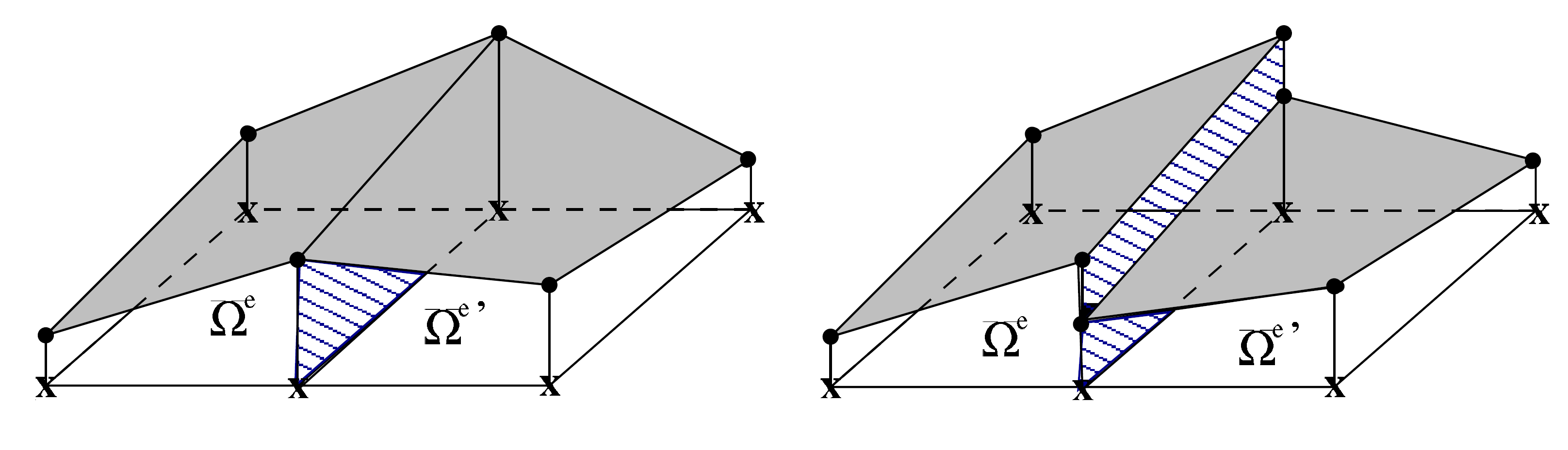
Figure 2. $C^{0}$ class elements and discontinuous ($C^{-1}$) elements.

In this case, the approximate solution ${\bm{u}}_{h}$ at a global node on $\Gamma$ will represent an intermediate value of the discontinuous solution. Our idea is to impose exactly the constraint

$$K_{1}^{-1}\bm{u}^{1}_{h}\cdot\tau=K_{2}^{-1}\bm{u}^{2}_{h}\cdot\tau$$ (6.6)

on the interface of discontinuity and assemble the global finite element approximation in terms of a reference solution $\bar{\bm{u}}_{h}$, which is uniquely defined at the nodes. This procedure leads a finite element formulation with the same connectivity of the global $C^{0}$ post-processing. We start by choosing as reference solution ${\bm{u}}^{2}_{h}$, such that

$$\bm{u}_{h}^{2}=\mathrm{I}\,\bar{\bm{u}}_{h}\quad\mbox{ on }\quad\Gamma\,,$$ (6.7)

where $\mathrm{I}$ is the identity. We now relate $\bm{u}_{h}^{1}$ to the reference solution. From Eqs (6.4) and (6.7) we can write

$$\mathrm{T}_{1}\bm{u}_{h}^{1}=\mathrm{T}_{2}\,\bm{u}_{h}^{2}=\mathrm{T}_{2}\,\bar{\bm{u}}_{h}\quad\mbox{ on }\quad\Gamma,$$

with the Cartesian matrix of $\mathrm{T}_{i}$ given by

$$\left[\mathrm{T}_{i}\right]=\left[\begin{array}[]{cc}\lambda_{11}^{i}\tau_{1}+\lambda_{21}^{i}\tau_{2}&\lambda_{12}^{i}\tau_{1}+\lambda_{22}^{i}\tau_{2}\\ \mathrm{n}_{1}&\mathrm{n}_{2}\end{array}\right]$$ (6.8)

where $(\tau_{1},\tau_{2})$ and $(\mathrm{n}_{1},\mathrm{n}_{2})$ are the Cartesian components of the unit vectors $\tau$ and $\bm{n}$, respectively, and $\lambda_{lm}^{i}$ are the components of the hydraulic resistivity tensor $\lambda_{i}=K_{i}^{-1}$. Considering that $\mathrm{T}_{1}$ is invertible, we get

$$\bm{u}_{h}^{1}=\mathrm{T}_{1}^{-1}\mathrm{T}_{2}\;\bar{\bm{u}}_{h}\quad\mbox{ on }\quad\Gamma.$$ (6.9)

Using Eqs (6.7) and (6.9) we are able to pose the interface problem in terms of a continuous global vector of unknowns $\{\bar{u}\}$ only. This can be done at element level as follows: let $\{u^{e}\}$ be the array of unknowns of a generic element $\Omega^{e}$ with just one edge belonging to the interface of discontinuity, and $\left\{u^{e}_{\Gamma}\right\}$ the unknowns associated with the nodes on that edge belonging to the interface. By using (6.9) to each node on $\Gamma$, we can construct a matrix $\left[\displaystyle T_{\Gamma}\right]$ and write

$$\left\{\displaystyle u^{e^{\,}}_{\Gamma}\right\}=\left[\displaystyle T_{\Gamma}\right]\{\displaystyle u^{e^{\prime}}_{\Gamma}\}$$ (6.10)

where $\Omega^{e}$ and $\Omega^{e^{\prime}}$ are elements that share the interface of material discontinuity as illustrated in Fig 2. Choosing $\{u^{e^{\prime}}_{\Gamma}\}$ as reference we have

$$\left\{u^{e}\right\}=\left\{\begin{array}[]{c}\left\{u^{e}_{\bar{\Omega}\backslash\Gamma}\right\}\\ ---\\ \left[\displaystyle T_{\Gamma}\right]\{\displaystyle u^{e^{\prime}}_{\Gamma}\}\end{array}\right\}=\left[T\right]\left\{\begin{array}[]{c}\left\{u^{e}_{\bar{\Omega}\backslash\Gamma}\right\}\\ ---\\ \{\displaystyle u^{e^{\prime}}_{\Gamma}\}\end{array}\right\}$$

or

$$\left\{u^{e}\right\}=\left[T\right]\{\bar{u}^{e}\}$$ (6.11)

where $[T]$ is the matrix of the linear transformation from $\{u^{e}\}$ to $\{\bar{u}^{e}\}$. The contribution of the element $\Omega^{e}$ to the global stiffness $[K]$ is given by:

$$[K^{e}]\{u^{e}\}=[K^{e}][T]\{\bar{u}^{e}\}=[\bar{K}^{e}]\{\bar{u}^{e}\},$$

with the new matrix $[\bar{K}^{e}]$ non-symmetric. The continuous/discontinuous approximation $\{u^{e}\}$ on the interface is obtained at element-level using (6.11) after solving the global system in $\{\bar{u}\}$.

Remarks.

1. In (6.8) we used unit vectors $\tau$ and $\bm{n}$ calculated at a nodal point on the interface. Using isoparametric elements, the interface $\Gamma$ is approximated by a interpolant $\Gamma_{h}\in C^{0}(\Gamma)$. In general, for curved interfaces these vectors are not uniquely defined at the vertices of the elements. In this case averages of these unit vectors can be adopted.

2. Considering that the solution of our model problem is piecewise smooth, we should expect that the error estimate (6.3) holds for each subdomain $\Omega_{i}$ when the continuity/discontinuity constraints on the normal/tangential components of Darcy’s velocity are exactly imposed on the interface of the two media with different hydraulic conductivity. A convergence study is presented in Sec. 7.3 confirming the orders of convergence predicted in (6.3).

3. As the weak forms of the global post-processings are posed in finite element subspaces of ${H(\operatorname{div})}$, they allow the use of divergence based finite element spaces, such as Raviart-Thomas spaces, naturally accommodating discontinuities of the tangent components of the velocity field on the interface of the elements.

4. Although introduced for the Global Post-Processing formulation this idea can, of course, be applied to more general situations, as for example, to the stabilized mixed finite element methods introduced in [6, 17] or to the local post-processing introduced in [14].

6.3. Local Post-Processings with Interface of Discontinuity

A stabilized mixed formulation using totally discontinuous Lagrangian interpolations for both velocity and potential fields is presented and analyzed in [21, 19]. Stability is provided, for $k\geq 1$, by consistently adding to an originally unstable DG formulation least squares or adjoint residuals of Darcy’s law. For using discontinuos interpolation, the velocity degrees of freedom are eliminated at element level in favor of the potential degrees of freedom. After solving the global system corresponding to the potential, the velocity approximation is computed by a local (element by element) post-processing. As proved in [19], choosing equal order interpolations this stabilized mixed method leads to optimal orders of convergence for the pressure and to the suboptimal estimate for the velocity approximation

$$\|\bm{u}-\bm{u}_{h}\|\leq Ch^{k}\|p\|_{k+1}\quad\mbox{ for}\quad k\geq 1\,.$$

Taking advantage of the superconvergence of the gradient of the Galerkin finite element solution at special points in the interior of the elements, a local post-processing at element or macroelement level is presented in [14], using least squares residuals of both equilibrium equation and the irrotationality condition. Let $\mathcal{S}_{h}^{k}$ be triangular or quadrilateral Lagrangian finite element subspaces of $L^{2}(\Omega)$ consisting of piecewise polynomials of degree $k$ on each element. By construction, we take $\mathcal{S}_{h}^{k}$ of class $C^{0}$ in each macroelement but discontinuous on the macroelement boundaries. In the product space $\mathbb{M}_{h}=\mathcal{S}_{h}^{k}\times\mathcal{S}_{h}^{k}$ we consider the mesh-dependent bilinear form

$$b_{h}(\bm{u}_{h},\bm{v}_{h})=(\bm{u}_{h},\bm{v}_{h})_{h}+h^{2}(\operatorname{\mathrm{div}}\bm{u}_{h},\operatorname{\mathrm{div}}\bm{v}_{h})+h^{2}(\operatorname{curl}\bm{u}_{h},\operatorname{curl}\bm{v}_{h})\quad\forall\bm{v}_{h},\bm{u}_{h}\in\mathbb{M}_{h}\,,$$

where $(\cdot,\cdot)_{h}$ denotes that this term is evaluated using an appropriate numerical integration rule to account for the superconvergence of $\nabla p_{h}$, and define the following local post-processing technique

Problem LPP

For a given $p_{h}$, solution of Problem Ph, find $\bm{u}_{h}\in\mathbb{M}_{h}$ such that

$$b_{h}(\bm{u}_{h},\bm{v}_{h})=(\nabla p_{h},\bm{v}_{h})_{h}-h^{2}(f,\operatorname{\mathrm{div}}\bm{v}_{h})\quad\forall\bm{v}_{h}\in\mathbb{M}_{h}\,.$$

Stability and convergence of this local post-processing formulation is proved in [14]. For quadrilateral elements and $k>1$, optimal orders of convergence are proved for any macroelement configuration, including element by element post-processings, when the mesh-dependent term $(\cdot,\cdot)_{h}$ is computed using the $k\times k$ Gauss integration points where the finite element approximation of the gradient is superconvegent with

$$|\nabla p-\nabla p_{h}|_{h}\leq Ch^{k+1}\|p\|_{k+2}\,,\quad|\nabla q|_{h}=(\nabla q,\nabla q)^{1/2}_{h}\,.$$

For $k=1$ this post-processing is also stable and optimally convergent for any macroelement composed by at least two adjacent elements with a common edge. In these cases the bilinear form $b_{h}(\cdot,\cdot)$ defines the norm

$$|||\bm{u}_{h}|||=(b_{h}(\bm{u}_{h},\bm{u}_{h}))^{1/2}\quad\forall\bm{u}_{h}\in\mathbb{M}_{h}\,,$$

which is equivalent to the $[L^{2}(\Omega)]^{2}$-norm on $\mathbb{M}_{h}$. By usual arguments, we derive the estimate

$$|||\bm{u}-\bm{u}_{h}|||\leq C(|||\bm{u}-\bm{v}_{h}|||+|\nabla p-\nabla p_{h}|_{h})\quad\forall\bm{v}_{h}\in\mathbb{M}_{h}\,.$$

For regular solutions, the above estimate leads to the optimal orders of convergence

$$\|\bm{u}-\bm{u}_{h}\|\leq Ch^{k+1}\|\bm{u}\|_{k+1}\,,$$ (6.12)

for the post-processed velocity approximation, in $[L^{2}(\Omega)]^{2}$-norm. For problems with regular exact solutions concerning homogeneous and isotropic media, these optimal orders of convergence are confirmed in [14] in a large number of numerical experiments. An extension of this local post-processing for triangular elements is presented in [18], in the context of h-adaptive analysis of Poisson’s problem, using the superconvergence points identified by Babuska, Strouboulis, Upadhyay and Gangaraj in [15].

Our point here is the application of this local post-processing to an anisotropic porous media with an interface of material discontinuity. Contrary to the global $C^{0}$ post-processing, the local post-processing is posed in finite element subspaces of $[L^{2}(\Omega)]^{2}$ using Lagrangian interpolation which are discontinuous on the macroelement interfaces. Applied to porous media with an interface of discontinuity on the hydraulic conductivity, the local post-processing naturally accommodates discontinuities of the tangent component but it does not ensure continuity of the normal component of the velocity field on the macroelement interfaces. However, as it is a stable and variationally consistent formulation, we should expect optimal orders of convergence for sufficiently regular exact solutions on each subdomain $\Omega_{i}$, independently of the fact that the continuity/discontinuity constraints on the normal/tangential components of Darcy’s velocity are not exactly imposed on the interface of two media with different hydraulic conductivity. Numerical results presented in Sec. 7.4 confirm the optimal orders of convergence when the interface of discontinuity belongs to the interface of the macroelements. If the interface of discontinuity is put in the interior of a macroelement, the continuity/discontinuity constraints on the normal/tangential components of Darcy’s velocity can be exactly imposed using the method presented in Sec. 6.2. In Figure 3 we illustrate: (a) case where the interface belongs to the edges of two homogeneous macroelements, (b) case where the interface is put in the interior of a macroelement. Again, optimal orders of convergence should be expected for piecewise regular solutions. This fact is also confirmed numerically in Sec. 7.4.

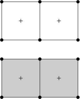
(a)

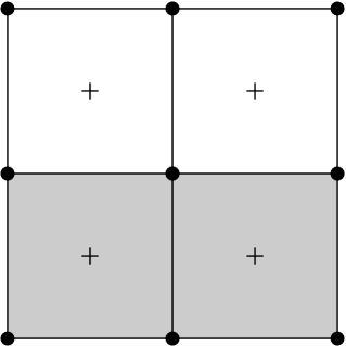
(b)

Figure 3. Stable macroelement configurations composed of bilinear quadrilaterals ($\bullet$, nodal points; +, superconvergent points): (a) two homogeneous macroelements composed by an arrange of $2\times 1$ bilinear quadrilaterals; (b) a macroelement of $2\times 2$ elements with interface of discontinuity. In this last case, the method described in Section 6.2 is adopted inside the macroelement

7. Numerical Examples

In this section, we present examples of applications of the proposed post-processing techniques to Darcy flow in layered heterogeneous media and compare their results with stabilized mixed methods. The first three examples illustrate qualitative aspects of the approximations, while the last example test the predicted orders of convergence. In all simulations we adopted for the global post-processings, with or without interface of discontinuity, $\delta=1$ and $\alpha=1$. According to the numerical analysis presented in [14] $\alpha=1$ is the best choice leading to quasi optimal orders of convergence for the velocity approximation in $L^{2}$-norm, and $\delta>0$ is sufficient for stability.

7.1. Flow Between Parallel Plates

This simple example clearly shows the consequences of imposing $C^{0}$ continuity in problems with discontinuous solutions. Let $\Omega=[0,L]\times[0,H]$ be the longitudinal section of a heterogeneous porous medium composed by two regions with different conductivities, confined between two parallel plates of infinite extent, as shown in Fig 4.

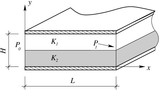
Figure 4. Domain.

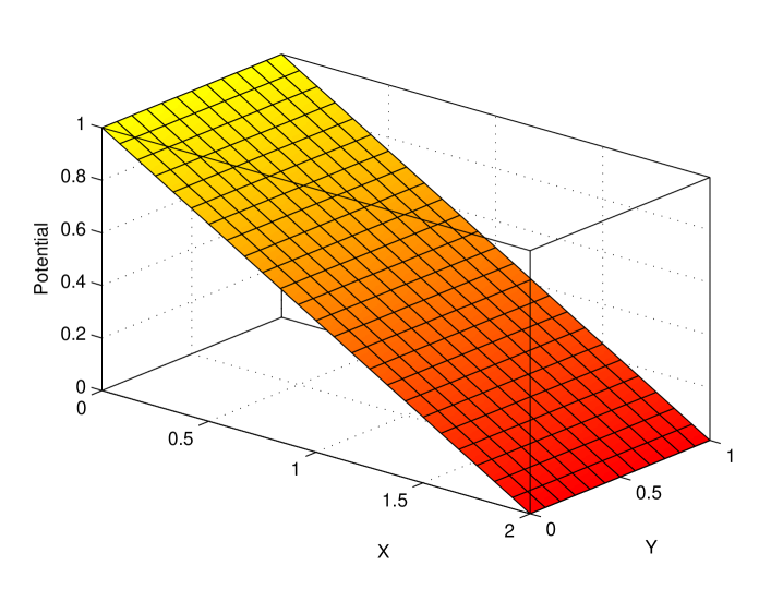
Figure 5. Approximated potential.

On the left extremity the hydraulic potential is prescribed $P_{0}=1.0$m and on the right extremity $P_{1}=0.0$m; on the plates we consider no-flux boundary conditions $\bm{u}\cdot\bm{n}=0$. The dimensions adopted are $L=2.0$m and $H=1.0$m, and the conductivities are $K_{1}=2.0\mathrm{m/day}$ and $K_{2}=1.0\mathrm{m/day}$. The flow is horizontal, originated by the gradient of potential $dp/dx=-0.5$, and the velocity can easily be calculated using Darcy’s law (3.2), yielding piecewise constant velocities $u_{1}=1.0\mathrm{m/s}$ in the upper region and $u_{2}=0.5\mathrm{m/s}$ in the lower one.

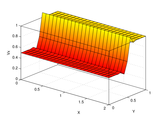
(a)

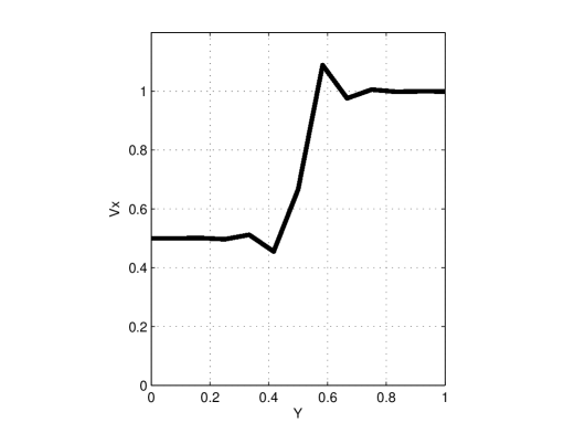
(b)

Figure 6. (a) HVM, GLS and GPP formulations: component $u_{x}$ of the approximated velocity. (b) Projection in $yz$ plane.

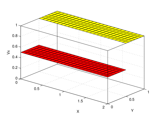
(a)

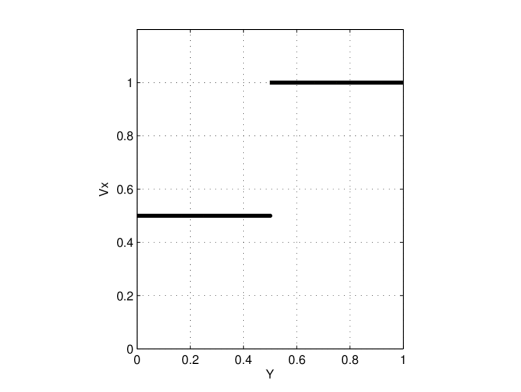
(b)

Figure 7. (a) Velocity approximated with GPPID, LPP and LPP with incorporated interface. (b) Projection in $yz$ plane.

First we consider $C^{0}$ approximations by the stabilized mixed methods: HVM and GLS (with $\delta_{1}=\delta_{2}=1/2$), and by the global $C^{0}$ post-processing (GPP). A uniform mesh of $24\times 12$ bilinear quadrilateral elements is adopted in all experiments. No difference was observed in the solutions obtained with these methods using $C^{0}$ velocity interpolations. Approximations for potential and velocity fields are shown in Figures 5 and 6, respectively. We can clearly observe spurious oscillations in the velocity approximation, as a consequence of imposing continuity. In contrast, in Fig 7 we present continuous/discontinuous velocity approximations obtained with: the global post-processing incorporating the discontinuity (GPPID), the local post-processing with $12\times 6$ homogeneous macroelements composed by arranges of $2\times 2$ bilinear quadrilaterals and the local post-processing with $6\times 3$ macroelements composed by arranges of $4\times 4$ elements, in which discontinuity/continuity constraints are introduced at macroelement level. The solution now is in perfect agreement with the real flow.

7.2. Flow With Less Pervious Barriers

This example, from Mosé et al. [11], simulates the flow in a porous media intersected by two less pervious barriers. These barriers force the flow to pass through a kind of channel. The boundary conditions are the same of the previous example. The geometry is detailed in Fig 8. The conductivities are $K_{1}=1.0$m/day for the porous media and $K_{2}=1.0\times 10^{-5}$m/day for the barriers.

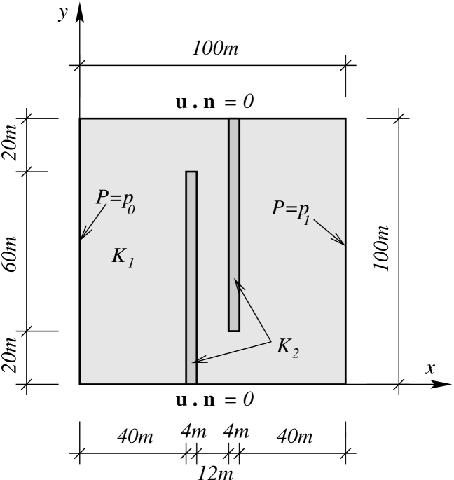
Figure 8. Domain.

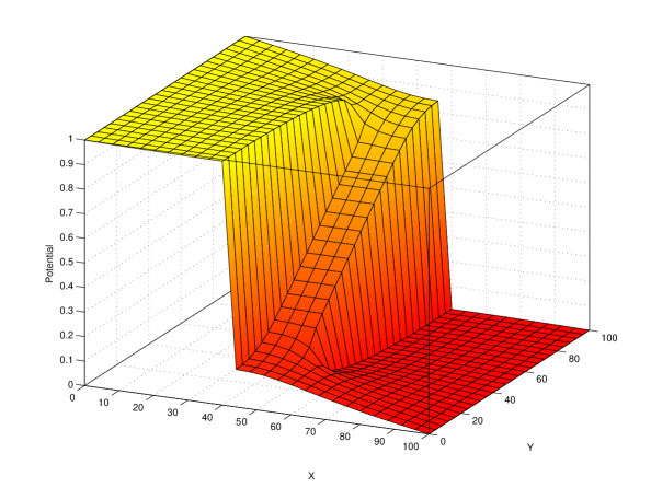
Figure 9. Approximated potential.

We approximated this problem by HVM and GPPID methods, using a uniform mesh of $25\times 25$ bilinear quadrilaterals. For GPPID, we assumed that at the corners with material discontinuity the relation $K_{1}^{-1}\bm{u}_{1}=K_{2}^{-1}\bm{u}_{2}$ holds. This is certainly a crude approximation for the interface conditions in which only the restriction on the tangential component is imposed. We should remind that in our model problem the interface is assumed to be smooth. This smoothness hypothesis is violated in this example.

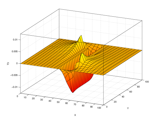
(a) HVM.

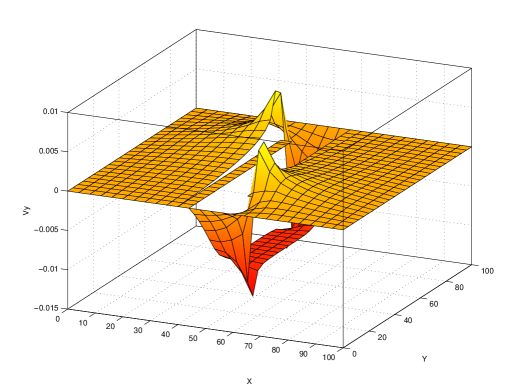
(b) GPPID.

Figure 10. Flow with less pervious barriers. Component $u_{y}$.

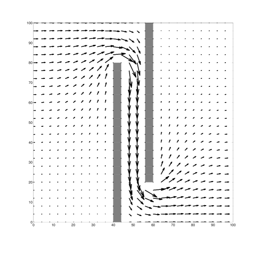
(a) Flow by HVM (There is artificial adherence on interface).

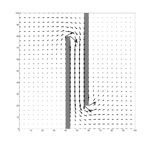
(b) Flow by GPPID (Tangent component well represented on interface).

Figure 11. Flow with less pervious barriers. Flow fields.

Figure 9 shows the Galerkin approximation for the potential. The potential approximated with HVM is similar. Figures 10a and 10b show the $u_{y}$ velocity component obtained with HVM and GPPID, respectively. We observe that the GPPID approximation capture the discontinuity. The flow calculated with HVM exhibits an artificial adherence to the barriers while the GPPID solution presents a behavior typical of no-flux condition, as we clearly observe in Figures 11a and 11b.

7.3. Porous Media with Three Different Conductivities

This is another example that does not fit in our model problem. Again we do not have a smooth interface of discontinuity. It is concerned with a heterogeneous porous media composed by three subdomains with different conductivities and two intersecting interfaces, as suggested by one of the referees. At the point of intersection it is not possible to assemble the nodal transformation (6.9). To handle this problem we adopted the local post-processing formulation using macroelements, naturally accommodating the interfaces of discontinuity on the macroelement edges or imposing the continuity/discontinuty constraints, through the nodal transformation (6.9), on interfaces interior to the macroelements.

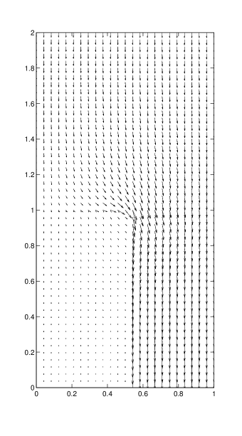
(a)

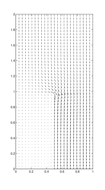
(b)

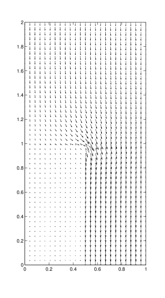
(c)

Figure 12. Flow through the porous media with three different conductivities. (a) Two (continuous) macroelements of $24\times 25$ elements, (b) interface in the interior of the first macroelement incorporated and (c) four macroelements of $12\times 25$ elements.

The domain of the problem is a rectangle given by the intervals $[0.0,1.0]\times[0.0,2.0]$ (lengths in meters), composed by three subdomains: the first defined on $[0.0,0.5]\times[0.0,1.0]$ with conductivity $K=1\mathrm{m/day}$, the second on $[0.5,1.0]\times[0.0,1.0]$ with $K=10\mathrm{m/day}$ and the third on $[0.0,1.0]\times[1.0,2.0]$ with $K=5\mathrm{m/day}$. The hydraulic potential is prescribed $P_{1}=1.0\mathrm{m}$ on the upper extremity and $P_{0}=0.0\mathrm{m}$ at the bottom; at the vertical boundaries we consider no-flux boundary conditions $\bm{u}\cdot\bm{n}=0$. The approximations were performed with a uniform mesh of $24\times 50$ bilinear quadrilaterals, composing the following arranges: (a) two macroelements of $24\times 25$ elements, where the interface between the first and the second subdomains is interior to the first macroelement, (b) four macroelements of $12\times 25$ elements; in this last case all interfaces belong to the set of edges of the macroelements.

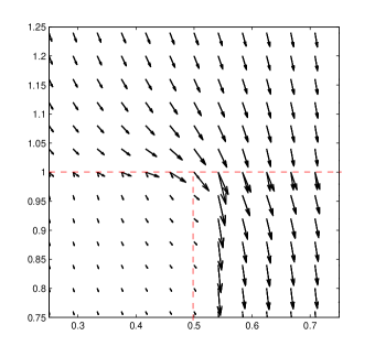
(a)

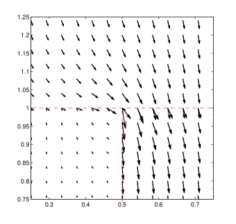
(b)

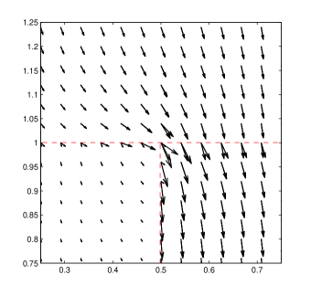
(c)

Figure 13. Details of the flow near to the point of intersection of the interfaces. (a) Two (continuous) macroelements, (b) two macroelements (ID) and (c) four macroelements.

In Figure 12a we show the flow for the approximation with 2 macroelements. In this case, the solution is continuous inside each macroelement. Adherence of the flow on the interface between the lower subdomains can be observed. A significant improvement on the flow approximation is achieved when we impose the interface conditions as shown in Fig 12b. The velocity on the interface is recovered. Similar results are obtained with the arrange of 4 macroelements with natural interface condition as presented in Fig 12c. Details of the flow near to the point of intersection of the interfaces are shown in Figures 13a, 13b, and 13c.

7.4. Convergence Study: An Anisotropic Heterogeneous Example

In this example we perform a convergence study in a general case where the conductivity tensor is anisotropic and heterogeneous. This test problem from Crumpton, Shaw and Ware [13] is defined on the square $[-1,1]\times[-1,1]$, with Dirichlet boundary conditions. The conductivity is given by

$$K=\left(\begin{array}[]{ccc}1&0\\ 0&1\end{array}\right)\quad x<0,\qquad K=\gamma\left(\begin{array}[]{ccc}2&1\\ 1&2\end{array}\right)\quad x>0,$$

where the parameter $\gamma$ is used to vary the strength of the discontinuity at $x=0$. In our experiments we used $\gamma=1.0$. The exact potential field is given by

$$p=\left\{\begin{array}[]{lcr}\gamma(2\sin(y)+\cos(y))x+\sin(y),&&x<0\\ \\ \exp(x)\sin(y),&&x>0\end{array}\right.$$

and the velocity field can be directly calculated by Darcy’s law. As in all formulations considered here the potential belongs to $\mathcal{Q}\in H^{1}(\Omega)$, we prescribe this variable on the boundary. The finite element solutions were computed adopting uniform meshes of $8\times 8$, $16\times 16$, $32\times 32$ and $64\times 64$ bilinear quadrilaterals (Q1) and $4\times 4$, $8\times 8$, $16\times 16$ and $32\times 32$ biquadratic quadrilaterals (Q2). In the specific convergence study for the local post-processing with interface of discontinuity in the interior of macroelements, we adopted uniform meshes of $6\times 6$, $12\times 12$, $24\times 24$ and $48\times 48$ Q1 elements, and $6\times 6$, $12\times 12$ and $24\times 24$ Q2 elements. To illustrate the different behaviors of continuous and discontinuous approximations, the $y$ components of the velocity fields obtained with $8\times 8$ bilinear quadrilaterals using HVM and GPPID are shown in Figures 14a and 14b, respectively.

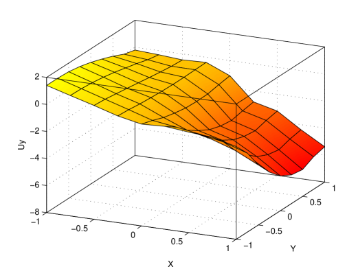
(a) HVM.

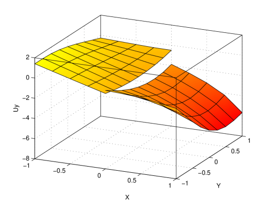
(b) GPPID.

Figure 14. Convergence study. Component $u_{y}$.

According to (6.3), for sufficiently regular solution we should expect the following orders of convergence

$$\|\bm{u}-\bm{u}_{h}\|\leq Ch^{k+0.5},\quad\|\operatorname{\mathrm{div}}\bm{u}-\operatorname{\mathrm{div}}\bm{u}_{h}\|\leq Ch^{k},$$

for the global $C^{0}$ post-processing with $\alpha=1$ and $\delta>0$. The error estimates for the other methods are given by Equations (5.7-5.9) for GLS, (5.11-5.13) for HVM and (6.12) for LPP. The point here is that the exact solution of this problem is not sufficiently regular in the whole domain $\Omega$, but regular enough in each subdomain $\Omega_{1}$ and $\Omega_{2}$, so that we can expect confirmation of the predicted orders of convergence whenever the discontinuity in the interface is appropriately captured. In the convergence graphics, we present plots of $L^{2}(\Omega)$ norm of the errors of the potential, velocity and its divergence versus $-\log(h)$. The label MACRO 2X2 (ID) in the pictures identifies approximations obtained with local post-processing with macroelements composed by $2\times 2$ elements with interface of discontinuity in the interior os macroelements (exactly imposed constraints), while MACRO 2X2 corresponds to approximations obtained with macroelements composed by $2\times 2$ homogeneous elements with the interfaces of discontinuties belonging to to the set of macroelement edges (constraints naturally accommodated). Again, we have adopted $\delta_{1}=\delta_{2}=1/2$ in the GLS formulation.

(a) Bilinear.

(b) Biquadratic.

Figure 15. Convergence of the velocity field.

Convergence results of velocity approximations for Q1 and Q2 elements are presented in Figures 15a and 15b, respectively. Convergence of $O(h^{0.5})$ is obtained for HVM and GLS methods for both Q1 and Q2 elements. It is consequence of the lack of global regurarity of the exact solution combined with the use of continuous interpolations to approximate a discontinuous field. The global post-processing with interface of discontinuity (GPPID) presents convergence orders typical of regular solutions: $O(h^{2.0})$ for Q1 and $O(h^{2.5})$ for Q2. Though not proved, the optimal convergence order of velocity in $L^{2}$ norm is usually observed for bilinear elements [14]. The results corresponding to the local post-processing (LPP) show the optimal orders: $O(h^{2.0})$ and $O(h^{3.0})$ for Q2, in agreement with the analysis of homogeneous problems with regular solutions.

(a) Bilinear.

(b) Biquadratic.

Figure 16. Convergence of the divergence of the velocity field.

Figures 16a and 16b present convergence results for the divergence of the velocity approximations in $L^{2}(\Omega)$-norm. The poor accuracy of GLS approximation for the velocity on the interface degradates the orders of convergence of its divergence. The same orders of convergence obtained for the velocity approximation in $L^{2}$-norm, close to $O(h^{0.5})$ for for both Q1 and Q2 elements, are observed for the divergence in the same norm. This result can be explained by estimate (5.6) for the GLS approximations in ${H(\operatorname{div})}$-norm for the velocity. Concerning HVM approximations, according to (5.12) we should not expect convergence for divergence using Q1 elements even for regular exact solutions, except for the “superconvergence” usually observed with linear and bilinear $C^{0}$ velocity approximations. But $O(h)$ convergence is expected with Q2 elements for regular solutions. However, no convergence is observed. This can be explicated by estimate (5.12) combined with the lack of global regularity of the exact solution of this model problem and the use of $C^{0}$ Lagrangian interpolation for the velocity field.

For exactly impose the constraints or naturally accommodate discontinuities on the interface, the convergence orders observed for GPPID and LPP are in agreement with those predicted by the numerical analysis.

(a) Bilinear.

(b) Biquadratic.

Figure 17. Convergence of the potential field.

Finally, in Figures 17a and 17b we plot the errors for potential using Q1 and Q2 elements, respectively. The Galerkin approximation, which is the starting point for the post-processings, shows the optimal orders predicted by (4.6), while the mixed methods show convergence orders of lower order than those we would expected from (5.7) for GLS and (5.11) for HVM. This can be explained by the coupled estimates for potential and velocity approximations characteristic of mixed methods ((5.6), for GLS, and (5.10), for HVM) and the lack of global regularity of the exact solution.

8. CONCLUSIONS

Stabilized mixed methods and global post-processings with $C^{0}$ Lagrangian interpolation present highly stable and accurate approximations for continuous velocity fields, as demonstrated and numerically confirmed in a large number of experiments [6, 9, 14, 16, 17, 22]. However, continuous interpolations are not adequate to approximate discontinuous velocity fields in heterogeneous porous media with an interface of material discontinuity. We proposed generalizations of global and local post-processing techniques, based on stabilized variational formulations, for Darcy flow in heterogeneous porous media with interfaces of discontinuities. By exactly imposing the continuity/discontinuity constraints on the interface of discontinuity we can recover stability, accuracy and the optimal of convergence of classical Lagrangian interpolations. Numerical results illustrate the performance of the proposed methods. Convergence studies for a heterogeneous and anisotropic porous medium with a smooth interface of discontinuity confirm the same orders of convergence predicted for homogeneous problem with smooth solutions, for both global and local post-processings. With the local post-processing, the continuity/discontinuity interface constraints can be exactly imposed in the interior of the macroelements or naturally accommodated on their edges. In both situations optimal orders of convergence were obtained.

References

- [1] Brezzi F. On the existence, uniqueness and approximation of saddle point problems arising from Lagrange multipliers. RAIRO Analyse numérique/Numerical Analysis 1974; 8(R-2):129–151.
- [2] Raviart PA, Thomas JM. A mixed finite element method for second order elliptic problems. In Math. Aspects of the FEM, Wunderlich W, Stein E, Bathe KJ (eds). Lectute Notes in Mathematics (606). Springer-Verlag, 1977; 292–315.
- [3] Ciarlet PG. The Finite Element Method for Elliptic Problems. North-Holland Publishing Company, 1978.
- [4] Loula AFD, Hughes TJ, Franca LP, Miranda I Mixed Petrov-Galerkin method for the Timoshenko beam. Comp. Meth. in App. Mech. and Eng. 1987; 63:133-154
- [5] Franca LP , Hughes TJ, Loula AFD, Miranda I. A New family of stable elements for nearly incompressible elasticity based on a mixed Petrov-Galerkin method . Numer. Math. 1988; 53:123-141
- [6] Loula AFD, Toledo EM. Dual and primal mixed Petrov-Galerkin finite element methods in heat transfer problems. Technical Report - LNCC 1988; 048/88.
- [7] Toledo EM. New Mixed Finite Element Formulations with Post-Processing (in Portuguese) 1990. DSc. Thesis - COPPE/UFRJ.
- [8] Brezzi F, Fortin M. Mixed and Hybrid Finite Element Methods. vol. 15. Springer-Verlag, New York, 1991.
- [9] Zienkiewicz, O.C. and Zhu, J.Z., The Superconvergent Patch Recovery and a posteriori error estimates. Part 1: The Recovery Technique. International Journal for Numerical Methods in Engineering 1992; 33, 1331-1364.
- [10] Cordes C, Kinzelbach W.. Continuous groundwater velocity fields and path lines in linear, bilinear and trilinear finite elements. Water Resources Research 1992; 28(11):2903–2911.
- [11] Mosé R, Siegel P, Ackerer P, Chavent G. Application of the mixed hybrid finite element approximation in a groundwater flow model: Luxury or necessity?. Water Resources Research 1994; 30(11):3001–3012.
- [12] Durlofsky LJ. Accuracy of mixed and control volume finite element approximations to Darcy velocity and related quantities. Water Resources Research 1994; 30(4):965–973.
- [13] Crumpton PI, Shaw GJ, Ware AF. Discretisation and multigrid solution of elliptic equations with mixed derivative terms and strongly discontinuous coefficients. Journal of Computational Physics 1995; 116:343–358.
- [14] Loula AFD, Rochinha FA, Murad MA. Higher-order gradient post-processings for second-order elliptic problems. Computer Methods in Applied Mechanics and Engineering 1995; 128:361–381.
- [15] Babuska I, Strouboulis T, Upadhyay T.C, S. Gangaraj S. Computer-Based Proof of the Existence of Superconvergence Points in the Finite Element Method; Superconvergence of the Derivatives in Finite Element Solutions of Laplace’s Poisson’s, and the Elasticity Equations, Numerical Methods for Partial Differential Equations 1996; 12:347–392.
- [16] Loula AFD, Garcia ELM, Coutinho ALG. Miscible displacement simulation by finite element method in distributed memory machines. Computer Methods in Applied Mechanics and Engineering 1999; 174:339–354.
- [17] Masud A, Hughes TJH. A Stabilized mixed finite element methods for Darcy Flow. Computer Methods in Applied Mechanics and Engineering 2002; 191:4341–4370.
- [18] Silva R.C.C, Loula A.F.D. Local residual error estimator and adaptive finite element analysis of Poisson’s problems. Computers & Structures 2002; 80:2027-2034.
- [19] Brezzi F, Hughes T.J.R, Marini, L.D, Masud, A. Mixed Discontinuous Galerkin Method for Darcy Flow. SIAM J. Scientific Comput. 2005; 22-23:119-145.
- [20] Dawson C. Coupling local discontinuous and continuous Galerkin methods for flow problems. Water Resources Research 2005; 28:729-744.
- [21] Hughes T.J.R, Masud, A, Wan J. A Stabilized mixed discontinuous Galerkin method for Darcy Flow. Computer Methods in Applied Mechanics and Engineering 2005; article in press.
- [22] Loula AFD, Correa MR Numerical Analysis of Stabilized Mixed Finite Element Methods For Darcy Flow ECCM2006, Lisbon, Portugal.