Endogenous Clustering and Analogy-Based Expectation Equilibrium

Abstract

Normal-form two-player games are categorized by players into K analogy classes so as to minimize the prediction error about the behavior of the opponent. This results in Clustered Analogy-Based Expectation Equilibria in which strategies are analogy-based expectation equilibria given the analogy partitions and analogy partitions minimize the prediction errors given the strategies. We distinguish between environments with self-repelling analogy partitions in which some mixing over partitions is required and environments with self-attractive partitions in which several analogy partitions can arise, thereby suggesting new channels of belief heterogeneity and equilibrium multiplicity. Various economic applications are discussed.

Keywords: Analogy-based Expectation Equilibrium, Prototype theory, K-means clustering.
JEL Classification Numbers: D44, D82, D90

1 Introduction

Many economists recognize that the rational expectation hypothesis that is central in solution concepts such as the Nash equilibrium is very demanding, especially in complex multi-agent environments involving lots of different situations (games, states or nodes, depending on the application). Several approaches have been proposed to relax it. When the concern with the hypothesis is that there are too many situations for players to fine tune a specific expectation for each such situation, a natural approach consists in allowing players to lump together situations into just a few categories, and only require that players form expectations about the aggregate play in each category.

The analogy-based expectation equilibrium (Jehiel, 2005) is a solution concept that has been proposed to deal with this. In addition to the usual primitives describing a game form, players are also endowed with analogy partitions, which are player-specific ways of partitioning situations or contingencies in the grand game. In equilibrium, the expectations in each analogy class correctly represent the aggregate behavior in the class, and players best-respond as if the behavior in every element of an analogy class matched the expectation about the aggregate play in the corresponding analogy class. This approach has been developed and applied to a variety of settings, but in almost all these developments, the analogy partitions are taken as exogenous (see Jehiel (2022) for a recent exposition of this strand of literature).

From a different perspective, psychologists have long recognized the use of categories to facilitate decision making and predictions (see, in particular, Anderson (1991) on predictions). For leading approaches in psychology (see in particular Rosch (1978)), categories bundle distinct objects that are viewed as sufficiently similar to warrant a similar treatment. Each category is associated with a prototype that can be viewed as a representative object, and categories are defined so that objects are assigned to the category with nearest prototype (see Posner and Keele (1968) or Reed (1972)).

From yet another perspective, the K-means clustering technique considered in Machine Learning has been widely used as a method to categorize large sets of exogenously given datapoints into a pre-specified number K of clusters (see Steinhaus (1957), Lloyd (1957) and MacQueen (1967)). From that perspective, datapoints are the primitives, and the clustering problem consists in partitioning the datapoints into K clusters with representative points for each cluster defined so that the original datapoints are best approximated by the representative points in their cluster. Solving the clustering problem (defined as deriving the variance-minimizing categorization, say) is hard (NP-complete), and practitioners most of the time rely on a simple algorithm to approximate its solution (see the end of Subsection 2.3 for a succinct exposition of the algorithm).

In this paper, we propose endogenizing the choice of partitions in the analogy-based expectation setting on the basis of the above basic principles. Specifically, we consider a strategic environment consisting of different normal form two-player games drawn by nature according to some prior distribution where we have in mind that the various games are played at many different times by many different subjects. In each of the normal form games $\omega\in\Omega$, player $j=1,2$ has the same action set $A_{j}$. An analogy partition for player $i$ takes the form of a partition of the set of games $\Omega$, which is used by player $i$ to assess the behavior of player $j$ in the various games. The data points accessible by players consist of the empirical frequencies of past play of the subjects assigned to the role of the opponent in the various games. To make sense of these data points, a subject assigned to the role of player $i$ is viewed as clustering these data points into an exogenously given (typically small) number $K$ of categories where $K$ can be related to the number of items human beings can remember in short-term memory (see Miller (1956) for pioneering research on this). At the end of the clustering stage, each game is assigned to the cluster with nearest opponent’s representative behavior and the representative behavior in a cluster is identified with the mean behavior of the opponent across the games assigned to the cluster. In a later stage, the relevant game $\omega$ becomes known to the subject, the player then identifies the behavior of his opponent in this game $\omega$ with the representative expectation in the corresponding cluster, and best-responds to it. This in turn generates new data points, and we are interested in the steady states - referred to as clustered analogy-based expectation equilibria - generated by such dynamic processes.

Roughly, the clustered analogy-based expectation equilibria (CABEE) can be described as profiles of analogy partitions and strategies such that i) given the analogy partitions, players’ strategies form an analogy-based expectation equilibrium and ii) given the strategies, clustering leads players to adopt the analogy partitions considered in steady state.

A key observation is that, in some cases, a steady state with a single analogy partition for each player does not exist. This follows because unlike in the usual clustering problem, there is here an extra endogeneity of the dataset. A change in analogy partitions may affect the adopted strategies through the working of the analogy-based expectation equilibrium, which in turn may affect how clustering is done. This will be first illustrated with a simple example involving three matching pennies games.

This observation leads us to extend the basic definition of CABEE to allow for distributions over analogy partitions defined so that each analogy partition in the support is required to solve (either locally or globally) the clustering problem for that player and the strategies, now parametrized by the chosen analogy partition, satisfy the requirements of the analogy-based expectation equilibrium appropriately extended to cope with distributions over analogy partitions. We refer to such an extension as a clustered distributional analogy-based expectation equilibrium (CD-ABEE).

We show that in finite environments (i.e. environments such that there are finitely many normal form games and finitely many actions for each player), there always exists at least one CD-ABEE. We also provide two learning dynamic models that give rise to CD-ABEE as steady states. In one of them, as informally described above, the learning subjects first cluster the raw data in each game before they are told (typically with a lag) which game applies to them. We note that when several analogy partitions are required in steady state, it implies that different subjects assigned to the role of the same player would end up categorizing the various games differently, despite being exposed to the same objective datasets. In the second learning model, subjects are told categories and representative points by their parents, then they play accordingly in the various games. In a later stage, subjects arrange newly observed behaviors in these games in new categories and pass these as well as the corresponding representative points to their off-springs.

We next consider various applications. A common theme that we consider throughout is whether the environment is such that starting from any candidate analogy partition profile, we obtain behaviors (through the machinery of ABEE) that would lead to the re-categorization of at least one game (through the machinery of clustering) or else whether the environment is such that starting from several (sometimes many) analogy partition profiles, we obtain (ABEE) behaviors that in turn lead to the same partition profile from the clustering perspective. We say that the environment has self-attractive analogy partitions in the latter case and self-repelling ones in the former. Environments with self-attractive analogy partitions suggest for such environments a novel channel through which different societies may settle down on different behaviors and different models of expectation formation. By contrast, environments with self-repelling analogy partitions lead to CD-ABEE (with mixed distributions of analogy partitions) and can be viewed as suggesting in such settings a new channel of heterogeneity in behaviors and expectation formation within societies.

We first provide an illustration of an environment with self-attractive analogy partitions in the context of beauty contest games in which players care both about being close to a fundamental value (which parametrizes the game) and being close to what the opponent is expected to be choosing. We show that the set of CABEE expands as the concern for coordination with the opponent increases. We also observe that when the coordination motive is sufficiently strong, virtually all analogy partitions of the fundamental value can be used to construct a CABEE, and as a result many different strategies can arise in a CABEE. The latter result illustrates in a very extreme way a case of self-attractive analogy partitions.

We next illustrate the possibility of self-repelling analogy partitions in the context of a monitoring game involving an employer who has to choose whether or not to exert some control and a worker who can be one of three possible types (which defines the game) and has to decide his effort attitude. When the employer can use two categories and only one minority type is responsive to the monitoring technology, we observe that heterogeneous categories are needed, thereby shedding new light on the study of discrimination in such applications.

Finally, we consider families of games with linear best-responses parametrized by the magnitude of the impact of opponent’s action on the best-response. We analyze separately the case of strategic complements and the case of strategic substitutes allowing us to cover applications such as Bertrand or Cournot duopoly with product differentiation, linear demand and constant marginal costs. We show that the strategic complements case corresponds to an environment with self-attractive analogy partitions and the strategic substitute case corresponds to an environment with self-repelling analogy partitions.

In the rest of the paper, we develop the framework (solution concepts, existence results, learning foundation) in Section 2. We develop applications in Section 3. We conclude in Section 4.

1.1 Related Literature

This paper belongs to a growing literature in behavioral game theory, proposing new forms of equilibrium designed to capture various aspects of misperceptions or cognitive limitations. While some papers in this strand posit some misperceptions of the players and propose a corresponding notion of equilibrium (see Eyster-Rabin (2005) on misperceptions about how private information affects behavior, Spiegler (2016) on misperceptions on the causality links between variables of interest or Esponda-Pouzo (2016) for a more abstract and general formulation of misspecifications), other papers motivate their equilibrium approach by the difficulty players may face when trying to understand or learn how their environment behaves (see Jehiel (1995) on limited horizon forecasts, Osborne-Rubinstein (1998) on sampling equilibrium, Jehiel (2005) on analogical reasoning or Jehiel-Samet (2007) on coarse reinforcement learning). Our paper has a motivation more in line with the latter, but it adds structure on the coarsening of the learning based on insights or techniques borrowed from psychology and/or machine learning (which the previous literature just mentioned did not consider).

This paper also relates to papers dealing with coarse or categorical thinking in decision-making settings (see, in particular, Fryer and Jackson (2008) for such a model used to analyze stereotypes or discrimination, Peski (2011) for establishing the optimality of categorical reasoning in symmetric settings or Al-Najjar and Pai (2014) and Mohlin (2014) for models establishing the superiority of using not too fine categories in an attempt to mitigate overfitting or balance the bias-variance trade-off). Our paper considers a clustering technique not discussed in those papers, and due to the strategic character of our environment the data-generating process in our setting is itself affected by the categorization, which these papers did not consider.

Finally, a contemporaneous and alternative approach to categorization in the context of the analogy-based expectation equilibrium is that introduced in Jehiel and Mohlin (2023) who propose putting structure on the analogy partitions based on the bias-variance trade-off where an exogenously given notion of distance between the various nodes or information sets is considered by the players. This is a different approach to categorization than the one considered in this paper, and it is more impactful in contexts such as extensive form games in which the behaviors in some nodes cannot be observed without trembles. In the context considered here with a set of normal form games (all arising with positive probability) it would lead to consider the finest analogy partition and accordingly the Nash Equilibrium would arise, in sharp contrast with the findings developed below.

2 Theoretical setup

2.1 Strategic environment

We consider a finite number of normal form games indexed by $\omega\in\Omega$ where game $\omega$ is chosen (by Nature) with probability $p(\omega)$. To simplify the exposition, we restrict attention to games with two players $i=1,2$, and we refer to player $j$ as the player other than $i$. In every game $\omega$, the action space of player $i$ is the same and denoted by $A_{i}$. It is assumed in this part to be finite. The payoff of player $i$ in game $\omega$ is described by a von Neumann-Morgenstern utility where $u_{i}(a_{i},a_{j},\omega)$ denotes the payoff obtained by player $i$ in game $\omega$ if player $i$ chooses $a_{i}\in A_{i}$ and player $j$ chooses $a_{j}\in A_{j}$. Let $p_{i}\in\Delta A_{i}$ denote a probability distribution over $A_{i}$ for $i=1,2$. With some abuse of notation, we let:

$$u_{i}(p_{i},p_{j},\omega)={\displaystyle\sum_{a_{i},a_{j}}}p_{i}(a_{i})p_{j}(a_{j})u_{i}(a_{i},a_{j},\omega)$$

denote the expected utility obtained by player $i$ in game $\omega$ when players $i$ and $j$ play according to $p_{i}$ and $p_{j}$, respectively.

We assume that players observe the game $\omega$ they are in when choosing their actions. A strategy for player $i$ is denoted $\sigma_{i}=\left(\sigma_{i}(\omega)\right)_{\omega\in\Omega}$ where $\sigma_{i}(\omega)\in\Delta A_{i}$ denotes the (possibly mixed) strategy employed by player $i$ in game $\omega$. The set of player $i$’s strategies is denoted $\Sigma_{i}$, and we let $\Sigma=\Sigma_{i}\times\Sigma_{j}$.

A Nash equilibrium is a strategy profile $\sigma=(\sigma_{i},\sigma_{j})\in\Sigma$ such that for every player $i$, $\omega\in\Omega$, and $p_{i}\in\Delta A_{i}$,

$$u_{i}(\sigma_{i}(\omega),\sigma_{j}(\omega),\omega)\geq u_{i}(p_{i},\sigma_{j}(\omega),\omega)\text{.}$$

2.2 Analogy-based expectation equilibrium

Players are not viewed as being able to know or learn the strategy of their opponent for each game $\omega$ separately as implicitly required in Nash equilibrium. Maybe because there are too many games $\omega$, they are assumed to learn the strategy of their opponent only in aggregate over collections of games, referred to as analogy classes. Throughout the paper, we impose that player $i$ considers (at most) $K_{i}$ different analogy classes, where $K_{i}$ is kept fixed. Such a bound can be the result of constraints on memory (see the introduction), and we will have in mind that $K_{i}$ is no greater and typically (possibly much) smaller than $\left|\Omega\right|$, the number of possible normal form games. We refer to $\mathcal{K}_{i}$ as the set of partitions of $\Omega$ with $K_{i}$ elements. Formally, considering for now the case of a single analogy partition for each player $i$, we let $An_{i}=\left\{\alpha_{i}^{1},\ldots,\alpha_{i}^{K_{i}}\right\}$ denote the analogy partition of player $i$. It is a partition of the set $\Omega$ of games with $K_{i}$ classes, hence an element of $\mathcal{K}_{i}$. For each $\omega\in\Omega$, we let $\alpha_{i}(\omega)$ denote the (unique) analogy class to which $\omega$ belongs.

$\beta_{i}(\alpha_{i})\in\Delta A_{j}$ will refer to the (analogy-based) expectation of player $i$ in the analogy class $\alpha_{i}$. It represents the aggregate behavior of player $j$ across the various games $\omega\;$in $\alpha_{i}$. We say that $\beta_{i}$ is consistent with $\sigma_{j}$ whenever for all $\alpha_{i}\in An_{i}$,

$$\beta_{i}(\alpha_{i})={\displaystyle\sum_{\omega\in\alpha_{i}}}p(\omega)\sigma_{j}(\omega)/{\displaystyle\sum_{\omega\in\alpha_{i}}}p(\omega)\text{.}$$

In other words, consistency means that the analogy-based expectations correctly represent the aggregate behaviors in each analogy class when the play is governed by $\sigma$. We say that $\sigma_{i}$ is a best-response to $\beta_{i}$ whenever for all $\omega\in\Omega$ and all $p_{i}\in\Delta A_{i}$,

$$u_{i}(\sigma_{i}(\omega),\beta_{i}(\alpha_{i}(\omega)),\omega)\geq u_{i}(p_{i},\beta_{i}(\alpha_{i}(\omega)),\omega)\text{.}$$

In other words, player $i$ best-responds in $\omega$ as if player $j$ played according to $\beta_{i}(\alpha_{i}(\omega))$ in this game, which can be viewed as the simplest representation of player $j$’s strategy given the coarse knowledge provided by $\beta_{i}$.

Definition 1

Given the strategic environment and the profile of analogy partitions $An=(An_{i},An_{j})$, $\sigma$ is an analogy-based expectation equilibrium (ABEE) if and only if there exists a profile of analogy-based expectations $\beta=(\beta_{i},\beta_{j})$ such that for each player $i$ (i) $\sigma_{i}$ is a best-response to $\beta_{i}$ and (ii) $\beta_{i}$ is consistent with $\sigma_{j}$.

This concept has been introduced with greater generality in Jehiel (2005) (allowing for multiple stages and more than two players) and in Jehiel and Koessler (2008) (allowing for private information). We have chosen a simpler environment to focus on the choice of analogy partitions, which is the main concern of this paper.

2.3 Clustering

Psychologists have long recognized the use of categories to facilitate decision making and predictions (see, in particular, Anderson (1991) on predictions). A categorization bundles distinct objects into groups or categories, whose members are viewed as sufficiently similar to warrant a similar treatment. In each category, there is a prototype that can be viewed as a representative element in the category (say the mean or the mode, see Rosch (1978)), and categories are defined so that objects are assigned to the category with nearest prototype (Posner and Keele (1968) or Reed (1972)). Another approach to categorization would require that objects are categorized so as to minimize some measure of dispersion such as the variance (or the relative entropy when objects can be identified with probability distributions, as in our environment).

In our framework, the objects considered by a subject assigned to the role of player $i$ consist of the frequencies of choices of the subjects assigned to the role of player $j$ in the various normal form games $\omega$ (this is made explicit when describing the learning environment, see section 2.6). That is, for player $i$, the objects are $\left\{(\omega,\sigma_{j}(\omega))\right\}_{\omega\in\Omega}$. An obvious attribute of $(\omega,\sigma_{j}(\omega))$ is the distribution of opponent’s behavior as described by $\sigma_{j}(\omega)$, and we will assume that player $i$ focuses on that attribute when choosing his categorization. This will in turn lead the chosen categorization to minimize (either locally or globally) the prediction error about the play of the opponent. This feature, we believe, would naturally be regarded as desirable by player $i$, as predicting the opponent play is the only thing player $i$ cares about to determine his best-response.

We first introduce a measure of closeness in the space of distributions over actions. Formally, for three distributions of player $j$’s play $p_{j}$, $p_{j}^{\prime}$ and $p_{j}^{\prime\prime}$ in $\Delta A_{j}$, we say that $p_{j}$ is less well approximated by $p_{j}^{\prime}$ than by $p_{j}^{\prime\prime}$ whenever $d(p_{j},p_{j}^{\prime})>d(p_{j},p_{j}^{\prime\prime})$ where $d$ is a divergence function that will either be the square of the Euclidean distance $d(p_{j},p_{j}^{\prime}\,)=\left\|p_{j}-p_{j}^{\prime}\right\|^{2}$ (as defined over $\left(\Delta A_{j}\right)^{2}$) or the Kullback-Leibler divergence applied to distributions $d(p_{j},p_{j}^{\prime})={\displaystyle\sum_{a_{j}}}p_{j}(a_{j})\ln\frac{p_{j}^{\,{}^{\,}}\left(a_{j}\right)}{p_{j}^{\prime}\left(a_{j}\right)^{\,}}$.

We next define two notions of clustering relating the analogy partition of player $i$ to the strategy of player $j$.

Definition 2

A partition $An_{i}$ of $\Omega$ is locally clustered with respect to $\sigma_{j}$ iff for all classes $\alpha_{i}$, $\alpha_{i}^{\prime}$ of $An_{i}$ and every $\omega\in\alpha_{i}$,

$$d(\sigma_{j}(\omega),\beta_{i}(\alpha_{i}))\leq d(\sigma_{j}(\omega),\beta_{i}(\alpha_{i}^{\prime}))\text{.}$$

It is globally clustered with respect to $\sigma_{j}$ iff $An_{i}\$belongs to

$$\arg\min_{P_{i}\in\mathcal{K}_{i}}{\displaystyle\sum_{c_{i}\in P_{i}}}p(c_{i}){\displaystyle\sum_{\omega\in c_{i}}}p(\omega\mid c_{i})d(\sigma_{j}(\omega),\beta_{i}(c_{i}))$$ (1)

where, for all $c\subseteq\Omega$, $\beta_{i}(c)=$ ${\displaystyle\sum_{\omega\in c}}p(\omega\mid c)\sigma_{j}(\omega)$.

In the above definition, $\beta_{i}(c)$ is viewed as the prototype in category $c$ and it is defined as the mean of the elements assigned to $c$. Local clustering retains the idea that objects should be assigned to the category with nearest prototype. Global clustering on the other hand requires that categorizations are chosen to minimize dispersion as measured by (1). When $d$ is the square of the Euclidean distance, the measure of dispersion corresponds to variance. When $d$ is the the Kullback-Leibler divergence, the measure of dispersion corresponds to relative entropy. We note that in both cases, choosing the prototype to be the mean of the elements assigned to the category is optimal (in the sense of minimizing the dispersion measure), thereby giving a further argument for using the mean as the prototype in our context.

It should be stressed (and as formally established in Lemma 1 in the Online Appendix B) that global clustering implies local clustering for the $d$ as specified above. As it turns out, the local clustering conditions can be viewed as the first order conditions for the minimization problem (1).

Link to K-means clustering.

In Machine Learning, a very popular way to categorize objects is based on the K-means clustering algorithm (Steinhaus (1957), Lloyd (1957) and MacQueen (1967)). The objective of clustering is also to minimize variance (or relative entropy) as considered in our global clustering approach, but this is known to be NP hard in computer science. Practitioners instead use the following algorithm. Representative points are initially drawn, then at each subsequent iteration of the algorithm, first points are allocated to the cluster with closest representative, then, a new representative point, identified with the mean of the points allocated to the cluster, is determined in each cluster. Such an algorithm can be shown to converge, and it turns out that it necessarily converges to a local minimizer of the dispersion measure. Moreover, all local minimizers satisfy the local clustering condition requiring that points are assigned to the cluster with closest representative point.

2.4 Clustered analogy-based expectation equilibrium

Combining Definitions 1 and 2 yield:

Definition 3

A pair $(\sigma,\,An)$ of strategy profile $\sigma=(\sigma_{i},\sigma_{j})$ and analogy partition profile $An=(An_{i},An_{j})\in\mathcal{K}_{i}\times\mathcal{K}_{j}$ is a locally (resp. globally) clustered analogy-based expectation equilibrium iff (i) $\sigma$ is an analogy-based expectation equilibrium given $An$ and (ii) for each player $i$, $An_{i}$ is locally (resp. globally) clustered with respect to $\sigma_{j}$.

The more interesting and novel aspect in this definition is the fixed point element linking analogy partitions to strategies and vice versa. With respect to the previous papers (using the ABEE framework), it suggests a way to endogenize the analogy partitions (given the numbers $K_{i}$ and $K_{j}$ of allowed analogy classes). With respect to the clustering literature, the novel aspect is that the set of points to be clustered $\{\left(\omega,\sigma_{j}(\omega)\right)\}_{\omega\in\Omega}$ for player $i$ is itself possibly influenced by the shape of the clustering, as captured by the analogy-based expectation equilibrium.

When some player $i$ has a dominant strategy in all games $\omega\in\Omega$, there always exists a (locally or globally) clustered ABEE because player $j$’s analogy partition can simply be obtained by clustering on the exogenous dataset given by $i$’s dominant strategies. Also, if the number of games $\omega$ with different Nash equilibrium strategies is no larger than $K_{i}$ for each player $i$, a (globally) clustered ABEE is readily obtained by requiring that $i$ plays the corresponding Nash equilibrium strategy and games are bundled in the same analogy class only when the opponent’s strategies coincide in such games.

But, in general, a clustered analogy-based expectation equilibrium may fail to exist. We illustrate this in a context with three matching penny games with different parameter values assuming that one of the players can use only two categories.

Example 1. Let $x=a,b,c$, with $0<a<b<c<2$. The following three games are played, each with probability $\frac{1}{3}$. The corresponding payoff matrices are given by:

$$\begin{array}[]{ccc}G_{x}&L&R\\ U&(1+x,0)&(0,1)\\ D&(0,1)&(1,0)\end{array}$$

Proposition 1

Assume that $K_{1}=2$ and $K_{2}=3$, and $d$ is the square of the Euclidean distance in the space of probability distributions on $\left\{L,R\right\}$. There is no Clustered ABEE.

Roughly, Proposition 1 can be understood as follows. Matching pennies games are such that the Nash equilibrium involves some mixing. When the Row player puts two games $x$ and $x^{\prime}$ in the same analogy class, she can be mixing in at most one of these games (this is so because the incentives of Row are different in the two games and Row makes the same expectation about Column in both $x$ and $x^{\prime}$ when these belong to the same analogy class). This in turn induces some polarization of the behaviors of both players in the two games $x$ and $x^{\prime}$, which when $a,b$ and $c$ are not too far apart leads the Row player to re-categorize one of the two bundled games $x$ or $x^{\prime}$ with the left alone game $x^{\prime\prime}\neq x,x^{\prime}$ at the clustering stage. Details appear in Appendix.

2.5 Clustered distributional analogy-based expectation equilibrium

We address the existence issue by allowing players to use heterogeneous analogy partitions. Formally, the analogy partition $An_{i}$ of player $i$ may now take different realizations in $\mathcal{K}_{i}$, and we refer to $\lambda_{i}$ as the distribution of $An_{i}$ over $\mathcal{K}_{i}$. The distributions of analogy partitions of the two players are viewed as independent of one another (formalizing a random assignment assumption, see below the section on learning). We refer to $\lambda=(\lambda_{i},\lambda_{j})$ as the profile of these distributions, and we let $\Lambda=\Delta\mathcal{K}_{i}\times\Delta\mathcal{K}_{j}$ be the set of $(\lambda_{i},\lambda_{j})$. For each analogy partition $An_{i}$ of player $i$ in the support of $\lambda_{i}$ referred to as $Supp\lambda_{i}$, we let $\sigma_{i}(\cdot\mid An_{i}):\Omega\rightarrow\Delta A_{i}$ refer to the mapping describing how player $i$ with analogy partition $An_{i}$ behaves in the various games $\omega\in\Omega$. We refer to $\sigma_{i}=(\sigma_{i}(\cdot\mid An_{i}))_{An_{i}\in\mathcal{K}_{i}}$ as player $i$’s strategy, and we let $\sigma=(\sigma_{i},\sigma_{j})$ denote the strategy profile, the set of which is still denoted $\Sigma$.

Given $\lambda\in\Lambda$ and $\sigma\in\Sigma$, we can define the aggregate behaviors of the two players in each game, as aggregated over the various realizations of analogy partitions. For player $j$ in game $\omega$, this aggregate strategy can be written as:

$$\overline{\sigma}_{j}(\omega)={\displaystyle\sum_{An_{j}\in\mathcal{K}_{j}}}\lambda_{j}(An_{j})\sigma_{j}(\omega\mid An_{j}).$$ (2)

Let $\bar{\sigma}=(\bar{\sigma}_{i},\bar{\sigma}_{j})$ denote a profile of aggregate strategies and let $\overline{\Sigma}$ denote the set of such profiles.

The analogy-based expectation of player $i$ defines for each analogy partition $An_{i}\in$ $Supp\lambda_{i}$ and each analogy class $\alpha_{i}\in An_{i}$, the aggregate behavior of player $j$ in $\alpha_{i}$ denoted by $\beta_{i}(\alpha_{i}\mid An_{i})\in\Delta A_{j}$ (the dependence on $An_{i}$ is here to stress that player $i$ with analogy partition $An_{i}$ considers only the aggregate behaviors in the various analogy classes in $An_{i}$). Similarly as above, $\beta_{i}(\cdot\mid An_{i})$ is said to be consistent with $\overline{\sigma}_{j}$ iff, for all $\alpha_{i}\in An_{i}$,

$$\beta_{i}(\alpha_{i}\mid An_{i})={\displaystyle\sum_{\omega\in\alpha_{i}}}p(\omega)\overline{\sigma}_{j}(\omega)/{\displaystyle\sum_{\omega\in\alpha_{i}}}p(\omega)\text{.}$$ (3)

We are now ready to propose the distributional extensions of our previous definitions.

Definition 4

Given $\lambda=(\lambda_{i},\lambda_{j})\in\Lambda$, a strategy profile $\sigma=(\sigma_{i},\sigma_{j})\in\Sigma$ is a distributional analogy-based expectation equilibrium (ABEE) iff there exists $\beta=(\beta_{i},\beta_{j})$ such that for every player $i$ and $An_{i}\in Supp\lambda_{i}$, we have that i) $\sigma_{i}(\cdot\mid An_{i})$ is a best-response to $\beta_{i}(\cdot\mid An_{i})$ and ii) $\beta_{i}(\cdot\mid An_{i})$ is consistent with $\overline{\sigma}_{j}$ (where $\overline{\sigma}_{j}$ is derived from $\sigma_{j}$ as in (2)).

Definition 5

A pair $(\sigma,\lambda)\in\Sigma\times\Lambda$ is a locally (resp. globally) clustered distributional analogy-based expected equilibrium iff i) $\sigma$ is a distributional ABEE given $\lambda$, and ii) for every player $i$ and $An_{i}\in Supp\lambda_{i}$ (where $\lambda=(\lambda_{i},\lambda_{j})$), $An_{i}$ is locally (resp. globally) clustered with respect to $\overline{\sigma}_{j}$ (where $\overline{\sigma}_{j}$ is derived from $\sigma_{j}$ as in (2)).

Clearly, a clustered distributional ABEE coincides with a clustered ABEE if the distributions of analogy partitions assign probability 1 to a single analogy partition for both players $i$ and $j$. Clustered distributional ABEE are thus generalizations of clustered ABEE. We now establish an existence result.

Theorem 1

In finite environments, there always exists a locally (resp. globally) clustered distributional ABEE when $d$ is the square of the Euclidean distance or the Kullback-Leibler divergence.

We prove this result by making use of Kakutani’s fixed point theorem. Details appear in Appendix. An implication of clustered distributional ABEE that would involve several analogy partitions is that different subjects exposed to the same objective datasets (and the same memory constraints as summarized by the number of allowed categories) may end up choosing different analogy partitions. Such a motive for an heterogeneous way of processing the same objective dataset is a consequence of the link between the categorizations and the datasets (through ABEE) and it has no analog in the literature.

2.6 Learning foundation

We suggest two learning interpretations of our proposed solution concepts. Each learning model involves populations of players randomly matched to play the various games and two distinct stages. In our first learning model, subjects are exposed to raw data about aggregate behaviors in each of the possible games in the first stage. In this stage, they do not know yet the game that will apply to them. To make sense of the data, they run a clustering of the raw data into $K$ clusters, which they then use in the second stage to adjust a best-response when they know the game they are in. In the second learning model, which has elements of a model of cultural transmission, in the first stage, subjects inherit categories with corresponding representative behaviors from their parents and they best-respond to the coarse feedback in the games that apply to them. In a second stage, the newly generated data about the plays in the various games are observed, and these are re-arranged in new categories and representative behaviors to be passed to the offspring. The steady states of these learning models correspond to clustered distributional ABEE.

Learning model 1 (Raw data and Machine Learning)

Consider the following learning environment. There are populations of mass 1 of subjects assigned to the roles of player $1$ and $2$. At all time periods $t$ except the first one, there are two stages.

• In stage 1, subjects assigned to the role of player $i$ see the datasets
  $\left\{(\omega,\overline{\sigma}_{j}^{t-1}(\omega))\right\}_{\omega\in\Omega}$, where $\overline{\sigma}_{j}^{t-1}(\omega)$ denotes the aggregate frequencies of actions chosen at $t-1$ (and only at $t-1$) by the subset of subjects assigned to the role of player $j$ when the game was $\omega$. We consider the possibility of measurement error by which we mean that each observation $\overline{\sigma}_{j}^{t-1}(\omega)$ may be perturbed by a (small) subject-specific idiosyncratic term. Every subject $i$ implements a clustering of his dataset into $K_{i}$ categories. That is, he either implements a solution to (1) or he finds a local solution to this problem (say resulting from the implementation of the K-means algorithm). At the end of this, a subject is able to recognize to which category/analogy class $\alpha_{i}^{t}(\omega)$ a game $\omega$ is assigned as well as the representative point $\beta_{i}^{t}(\alpha_{i}^{t}(\omega))$ in $\alpha_{i}^{t}(\omega)$ defined as the mean of the elements assigned to $\alpha_{i}^{t}(\omega)$.

• In stage 2, subjects are randomly matched and each subject is informed of the game $\omega$ he is in. He then expects that the subject $j$ he is matched with will play according to $\beta_{i}^{t}(\alpha_{i}^{t}(\omega))$, which is the representative behavior in the analogy class to which $\omega$ has been assigned. Subject $i$ plays a best-response to this expectation. At the best-response stage, we consider the possibility of small perturbations in the payoff specifications as is commonly assumed in learning models (Fudenberg and Kreps, 1993).

In the Online Appendix A, we establish that the dynamic model just proposed admits steady states. Moreover, when subjects solve the full clustering problem (i.e., solving (1) in stage 1), we show that the limit of these steady states as the measurement error and the payoff perturbations vanish correspond to the globally clustered distributional ABEE. These results provide a learning foundation for the globally clustered distributional ABEE.

It should be stressed that our learning model implicitly requires that there is some lag between stage 1 and stage 2 so that subjects cannot in stage 2 go back to the raw data that correspond to the games they are in. In some sense, the categorization and clustering outcome can be viewed as representing how a constrained memory could pass information from the stage in which the raw data are available but the relevant game is not known to the stage in which the game is known and an action has to be chosen.

Learning model 2 (Categories, Representative Behaviors and Cultural Transmission)

Our second learning model involves dynasties of subjects. For each role $i$, each subject in the population assigned to role $i$ is viewed as belonging to a different dynasty. At the start of period $t$ and in each dynasty, the subject who acted at $t-1$ (the predecessor) is replaced by a successor who receives the categories and representative points from the predecessor. That is, each subject assigned to role $i$ receives some partition $An_{i}$ and representative points $(\beta_{i}^{t-1}(\alpha))_{\alpha\in An_{i}}$ from his respective predecessor. The share of subjects at time $t-1$ selecting $An_{i}$ in the population assigned to role $i$ is given by $\lambda_{i}^{t-1}(An_{i})$. Then at time $t$, the following two stages take place.

• In stage 1, each subject $i$ plays several games $\omega$, being randomly re-matched each time with subjects in the role of $j$. Each time subjects best-respond based on the inherited expectations $((\beta_{i}^{t-1}(\alpha))_{\alpha\in An_{i}}$.

• In stage 2, all subjects in the role of $i$ observe the behaviors in stage 1 of all subjects in the role of $j$ in all games $\omega$. They compute $\bar{\sigma}_{j}^{t}(\omega)$ for each $\omega$ and they assign games to the closest representative point $\beta_{i}^{t-1}(\alpha)$, selecting a possibly new partition based on the local clustering criterion. Then, a subject selecting the partition $An_{i}$ computes the representative points $((\beta_{i}^{t}(\alpha))_{\alpha\in An_{i}}$ to be consistent with $\bar{\sigma}_{j}^{t}$. The share of subjects selecting partition $An_{i}$ in the population determines the new shares $\lambda_{i}^{t}(An_{i})$. Each subject passes on the selected partition $An_{i}$ and the representative points to their successor within the dynasty.

While an explicit study of such a dynamic would require further work, it is readily verified that the corresponding steady states correspond to the locally clustered distributional ABEE.^,

3 Applications

In this Section we consider various applications. We focus throughout on whether the environment has multiple self-attractive analogy partitions or only self-repelling analogy partitions. In the former case, several choices of analogy partitions may lead to behaviors (through the machinery of ABEE) that agree (form the clustering perspective) to the initial choice of analogy partitions. In the latter case, any choice of analogy partitions leads to behaviors (through the machinery of ABEE) in at least one game that would have to be reallocated to another analogy class (from the clustering perspective).

While the matching penny environment discussed above gives an illustration of an environment with self-repelling analogy partitions, we will cover more applications in which this arises. We will also illustrate that the polar case of self-attractive analogy partitions can arise in classic environments, thereby suggesting a novel source of multiplicity of equilibria in such cases.

3.1 Self-Attractive Analogy Partitions: A Beauty Contest Game Illustration

We consider a family of games that induce strategic behavior in the spirit of the “beauty contest” example mentioned in Keynes’s General Theory (1936). These games are similar to those introduced in Morris and Shin (2002) except that in our setting there is no private information and players form their expectations in a coarse way.

Formally, a fundamental value (playing the role of the state in the above setting) can take values $\theta\$in $\Theta\subset\mathbb{R}$ and $\theta$ is assumed to be distributed according to some smooth density $f(\cdot)$ on $\Theta$. Player $i$ has to choose an action $a_{i}\in\mathbb{R}$.

When the fundamental value is $\theta$, player $i$ ’s utility is

$$U_{i}(a_{i},a_{-i};\theta)=-(1-r)(a_{i}-\theta)^{2}-r(a_{i}-a_{j})^{2},$$

where $0<r<1$. In other words, players would like to choose an action that is close both to the fundamental value and to the action chosen by the opponent where $r$ measures the weight attached to the latter and $1-r$ the weight attached to the former. It is the coordination aspect (i.e. $r>0$) that gives to this game the flavor of the beauty contest game.

As in the framework of Section 2, players are assumed to observe $\theta$. The quadratic loss formulation implies that if player $i$ expects $j$ to play according to the distribution $\sigma_{j}\in\Delta\mathbb{R}$ the best-response of player $i$ in game $\theta$ is

$$BR(\theta,\sigma_{j})=(1-r)\theta+rE(a_{j}\mid\sigma_{j}).$$

The unique Nash Equilibrium in game $\theta$ requires then that

$$a_{1}^{NE}(\theta)=a_{2}^{NE}(\theta)=\theta.$$

Consider now this same environment assuming players use $K$ categories as in Section 2. Given the symmetry of the problem, we focus on symmetric equilibria in which players $1$ and $2$ would both choose the same analogy partition $(\Theta_{k})_{k=1}^{K}$, and we let for each $k$

$$\overline{\theta}_{k}=E(\theta\mid\theta\in\Theta_{k})$$

denote the mean of the fundamental values conditional on $\theta$ lying in the analogy class $\Theta_{k}$. Straightforward calculations (detailed for completeness in the online Appendix B) show that there is a unique analogy-based expectation equilibrium such that for $\theta\in\Theta_{k}$:

$$a_{1}^{ABEE}(\theta)=a_{2}^{ABEE}(\theta)=(1-r)\theta+r\overline{\theta}_{k}.$$ (4)

In this equilibrium, players do not choose the fundamental value $\theta$ because their coarse expectation leads them to expect the mean action of the opponent to be $\overline{\theta}_{k}$ and not $\theta$ when $\theta\in\Theta_{k}$.

Assume that players use the square of the Euclidean distance applied to the mean of the distribution for clustering purposes. That is, the prediction error measure between the behavior of player $j$ in $\theta$ and the aggregate behavior of player $i$ in the the subset $\Theta_{k}^{\prime}$ is given by $(a_{j}^{ABEE}(\theta)-E(a_{j}^{ABEE}(\theta^{\prime})\mid\theta^{\prime}\in\Theta_{k}^{\prime}))^{2}$.

Our main insight is the observation that there are many possible clustered analogy-based expectation equilibria when the concern for coordination is large enough. More precisely,

Proposition 2

Take any partition $(\Theta_{k})_{k=1}^{K}$ such that $\overline{\theta}_{k}=E(\theta\mid\theta\in\Theta_{k})$ are all different. Then for $r$ sufficiently close to $1$, when both players use this analogy partition and play according to (4), we have a Clustered Analogy-based Expectation Equilibrium.

Proof. When $r$ is close to 1, actions $a_{j}^{ABEE}(\theta)$ in $\Theta_{k}$ are all close to $\overline{\theta}_{k}$. When $\overline{\theta}_{k}$ are all distinct, the clustering (whether local or global) leads to $(\Theta_{k})_{k=1}^{K}$. Q.E.D.

In other words, our beauty contest game illustrates in a stark way the possibility of self-attractive analogy partitions. When $r$ is close to $1$, virtually all analogy partitions can be sustained as part of a clustered ABEE. Or to put it differently: Once the analogy partition $(\Theta_{k})_{k=1}^{K}$ is chosen and no matter what this partition is, players are led through the working of the ABEE to behave in a way that makes the clustering into $(\Theta_{k})_{k=1}^{K}$ best for the purpose of minimizing prediction errors. Observe that the vast multiplicity of analogy partitions so derived results in a vast range of possible equilibrium behaviors as well, where behaviors are concentrated around the various $\bar{\theta}_{k}$.

Of course, we should not expect to have such an extreme form of self-attraction for all parameter values of the beauty contest game. For example, when $r$ is small (close to $0$), then behaviors are not much affected by the analogy partition, and in the limit as $r=0$, the only globally clustered ABEE would require choosing $(\Theta_{k})_{k=1}^{K}$ so as to minimize

$$\sum_{k=1}^{K}\int_{\Theta_{k}}(\theta-\overline{\theta}_{k})^{2}f(\theta)d\theta.$$

In the case $\theta$ is uniformly distributed on $\left[\underline{\theta},\overline{\theta}\right]$, this would lead to the equal splitting analogy partition (i.e., $\Theta_{k}=(\theta_{k-1},\theta_{k})$ where $\theta_{0}=\underline{\theta}$ and $\theta_{k}=\underline{\theta}+\frac{k}{K}(\overline{\theta}-\underline{\theta})$).

For intermediate values of $r$, we can support a bigger range of analogy partitions as part of a CABEE but not as many as when $r$ approaches $1$. The next Proposition establishes that as $r$ grows larger, more and more analogy partitions can be obtained.

Proposition 3

Take a partition $(\Theta_{k})_{k=1}^{K}$ and the corresponding ABEE for some $r<1$. Suppose this is a locally CABEE. Then, for any $r^{\prime}>r$, $(\Theta_{k})_{k=1}^{K}$ and the corresponding ABEE form a locally CABEE.

Proof. For each player $i$ note the following observations for a partition $(\Theta_{k})_{k=1}^{K}$. As $r$ increases, for each $\theta\in\Theta_{k}$, $a_{j}^{ABEE}(\theta)$ gets (weakly) closer to $\bar{\theta}_{k}$. Moreover if $\theta\in\Theta_{k}$ is weakly greater (resp. smaller) that $\bar{\theta}_{k}$, then:

(i) for each $\bar{\theta}_{k^{\prime}}>\bar{\theta}_{k}$ (resp. $<$), if the partition is locally clustered with respect to the corresponding ABEE for some $r<1$, then $a_{j}^{ABEE}(\theta)$ for $r^{\prime}>r$ is strictly further apart from $\bar{\theta}_{k^{\prime}}$ as compared to $a_{j}^{ABEE}(\theta)$ for $r$;

(ii) for each $\bar{\theta}_{k^{\prime}}\leq\bar{\theta}_{k}$ (resp. $\geq$), $a_{j}^{ABEE}(\theta)$ is weakly closer to $\bar{\theta}_{k}$ than $\bar{\theta}_{k^{\prime}}$ because $a_{j}^{ABEE}(\theta)$ is weakly greater (resp. smaller) than $\bar{\theta}_{k}$ for any $r$.

Thus, if $(\Theta_{k})_{k=1}^{K}$ is locally clustered with respect to $a_{j}^{ABEE}(\cdot)$ for given $r$, then it is also locally clustered with respect to $a_{j}^{ABEE}(\cdot)$ for any $r^{\prime}>r$. Q.E.D.

The insight of this Proposition can possibly be related to some features of echo chambers. When the concern for coordination is big, the clustering of fundamental values into analogy classes may not be much related to the objective realization of the fundamental values, and different societies (which may settle down on different CABEE) may end up forming different beliefs and adopting different behaviors in objectively identical situations.

The analysis presented here should be contrasted with insights obtained in the tradition of global games, suggesting a unique selection of equilibrium (see Morris and Shin (2002) for references). Of course, our setting is different (no private information), and our formalization of expectations through categories is also different, leading to alternative predictions and a novel perspective on the possibility of multiple equilibria. We believe that our finding that a larger variety of behaviors and larger departures from the fundamental can be obtained as agents are more concerned about coordinating with others agrees with Keynes’ intuition about beauty contests. While rational expectations in the beauty contest game would lead agents to adopt behaviors coinciding with the fundamental value, in our approach a much wider variety of behaviors and expectations can arise in such cases.

3.2 Self-Repelling Analogy Partitions: A Monitoring Game Illustration

Unless specified otherwise, the results stated in this subsection hold for $d$ being either the square of the Euclidean distance or the Kullback-Leibler divergence. We consider the following Employer-Worker environment. There are three types of workers $a,b,c$. An employer is matched with one worker who can be either of type $a$, $b$, or $c$ with probability $p_{a},p_{b},p_{c}$, respectively. The type $\omega=a,b,c$ of the worker is observed by the employer. It can be identified with the state in our general framework.

In each possible interaction $\omega$, the employer and the worker make simultaneous decisions. The employer decides whether he will Control ($C$) the worker or not ($D$). The worker decides whether to exert low effort $e=0$ or high effort $e=1$.

We assume that the employer cares about the type only through the effort attitude that she attributes to the type of worker. Specifically, we assume that the employer finds it best to choose $C$ only if she expects the worker to choose low effort with probability no less than $\nu^{\ast}$.

Workers’ effort attitudes depend on their type and possibly on their expectation about whether they will be controlled or not. Type $a$ of worker always chooses $e=0$ (irrespective of his expectation about the Control probability). Type $b$ always chooses $e=1$. Type $c$ of worker finds it best to exert low effort $e=0$ when he expects $C$ to be chosen with probability no more than $\mu^{\ast}$.

In the unique Nash equilibrium, the employer would choose $C$ when facing type $a$, $D$ when facing type $b$ and would mix between $C$ with probability $\mu^{\ast}$ and $D$ with probability $1-\mu^{\ast}$ when facing type $c$. Type $c$ of worker would choose $e=0$ with probability $\nu^{\ast}$.

Assuming the employer uses two categories $K=2$ whereas the worker is rational, we have:

Proposition 4

Assume $p_{c}$ is no larger than $p_{a}$ and $p_{b}$, $\frac{p_{c}}{p_{a}+p_{c}}<\nu^{\ast}<\frac{p_{b}}{p_{b}+p_{c}}$, and $\nu^{\ast}\neq\frac{p_{b}}{p_{a}+p_{b}}$. There is no pure Clustered Analogy-based expectation equilibrium in which a single analogy partition is used by the employer.

Proof. This is proven by contradiction. Let $\beta_{e=1}$ denote the probability attached to $e=1$ by the employer in her non-singleton analogy class. 1) If $ac$ are put together, consistency implies that $\beta_{e=1}$ is at most $\frac{p_{c}}{p_{a}+p_{c}}$, which is smaller than $\nu^{\ast}$. Best-response of the employer implies that $C$ (Control) is chosen when facing worker $c$. Best-response of the $c$-worker leads to $e_{c}=1$. The resulting profile of effort attitude is $(e_{a}=0,e_{b}=1,e_{c}=1)$, which leads at the clustering stage to reassign $c$ with $b$, thereby yielding a contradiction. 2) If $bc$ are put together, $\beta_{e=1}>\nu^{\ast}$ so that $D$ is chosen by the employer when facing the $c$-worker. This leads the $c$-worker to choose $e_{c}=0$ and the resulting profile of effort attitudes $(e_{a}=0,e_{b}=1,e_{c}=0)$ would lead to reassign $c$ to $a$, thereby leading to a contradiction. 3) If $ab$ are put together, $\beta_{e=1}=\frac{p_{b}}{p_{a}+p_{b}}$, and the probability that $e_{c}=1$ is $\nu^{\ast}$ (as the mixed Nash equilibrium is then played in the interaction with $c$). This violates the condition for local clustering, for either $a$ or $b$ whenever $\nu^{\ast}\neq\frac{p_{b}}{p_{a}+p_{b}}$. Q.E.D.

In other words, in this monitoring environment, any categorization is self-repelling, and steady state requires some mixing. When considering global clustering, we have:

Proposition 5

Assume $p_{c}$ is no larger than $p_{a}$ and $p_{b}$ and $\frac{p_{c}}{p_{a}+p_{c}}<\nu^{\ast}<\frac{p_{b}}{p_{b}+p_{c}}$. There is a unique globally Clustered Distributional ABEE in which the analogy partition putting $ac$ (resp. $bc$) together is chosen with probability $\mu^{\ast}$ (resp. $1-\mu^{\ast}$), the $c$ worker chooses $e=0$ and $1$ each with probability half, and the employer chooses $C$ in any analogy class containing $a$ and $D$ in any analogy class containing $b$.

This can easily be understood as follows. Given the choice of the Employer for each of her analogy partition, the distribution over analogy partitions is chosen so as to make the $c$ worker indifferent between his two effort options. The mixing of the $c$ worker is then chosen so as to make the two analogy partitions equally good for the purpose of minimizing the total variance (when $d$ is the square of the Euclidean distance) or the relative entropy (when $d$ is the Kullback-Leibler divergence). The rest of the construction follows easily.

One noteworthy aspect of the equilibrium is that $\nu^{\ast}$ plays no role in the equilibrium (so long as $\frac{p_{c}}{p_{a}+p_{c}}<\nu^{\ast}<\frac{p_{b}}{p_{b}+p_{c}}$). This is so because, in equilibrium, the employer is made indifferent between the two possible partitions at the clustering stage, but then her monitoring choice is deterministic for each analogy partition. Instead, Nash equilibrium prescribes that the employer is made indifferent between her monitoring options, thereby implying that the worker should exert effort $e=1$ with probability $\nu^{\ast}$.

Similar insights are obtained when local clustering is considered: a wider range of equilibria can be sustained, but in all of them, the analogy partition putting $ac$ (resp. $bc$) together must be chosen with probability $\mu^{\ast}$ (resp. $1-\mu^{\ast}$). The range of these depend on the probabilities $p_{\omega}$ of $\omega=a,b,c$ and to fix ideas, we consider in the next proposition that types $a$ and $b$ are equally likely.

Proposition 6

Assume that $p_{a}=p_{b}=p>\frac{1}{3}$, $\frac{p_{c}}{p_{a}+p_{c}}<\nu^{\ast}<\frac{p_{b}}{p_{b}+p_{c}}$, and $\nu^{*}\neq\frac{1}{2}$. The following defines the locally Clustered Distributional ABEE. The analogy partition putting $ac$ (resp. $bc$) together is chosen with probability $\mu^{\ast}$ (resp. $1-\mu^{\ast}$). The employer chooses $C$ in any analogy class containing $a$ and $D$ in any analogy class containing $b$. The $c$ worker chooses $e=0$ with probability $\zeta$ in the range $(p,\frac{1-p}{2-3p})$ when $d$ is the squared Euclidean distance and in the range $(0,1)$ when $d$ is the Kullback-Leibler divergence.

The main difference between the above two Propositions is that for local clustering, any mixing of the $c$ type that assigns probability $\zeta\in(p,\frac{1-p}{2-3p})$ on $e=0$ makes the two analogy partitions locally clustered with respect to the proposed strategy of the worker. Indeed, when the analogy partition putting $ac$ (resp. $bc$) together is considered, the aggregate effort distribution in $ac$ (resp. $bc$) assigns probability $\frac{p+(1-2p)\zeta}{1-p}$ (resp. $\frac{(1-2p)}{1-p}\zeta$) to $e=0$. When $d$ is the square of the Euclidean distance, the mixing $\zeta$ on $e=0$ is then closer to $\frac{p+(1-2p)\zeta}{1-p}$ (resp. $\frac{(1-2p)}{1-p}\zeta$) than to $0$ (resp. $1$) since $\zeta>p$ (resp. $\zeta<\frac{1-p}{2-3p}$). The Kullback-Leibler divergence is more permissive as it explodes to infinity when the support of the behavior is not contained in the support of the expectations. Then, any $\zeta\in(0,1)$ can be sustained because the behavior of $c$ worker assigns positive probability to both $e=1$ and $e=0$, while the expectations of the singleton classes only to one of the two.

With the above learning interpretation that involves populations of employers and workers, the observation that several analogy partitions must arise in a clustered distributional ABEE imply that not all employers categorize $c$ workers in the same way. This implies that different employers may have different beliefs about the working attitude of $c$ workers. Some employers (in proportion $\mu^{\ast}$) believe $c$ workers choose $e=0$ with probability $\frac{p+(1-2p)\zeta}{1-p}$ and others (in proportion $1-\mu^{\ast}$) believe $c$ workers choose $e=0$ with probability $\frac{(1-2p)}{1-p}\zeta$. That is, some overestimate the working attitude of $c$ workers and some underestimate it, leading in our model to polarized beliefs. Those employers underestimating the working attitude will treat the minority group ($c$ is the least likely type) exactly like type $a$, while the others will treat them exactly like type $b$. Even if stylized, we believe our analysis may provide a novel argument as to how different beliefs about the working attitude of minority groups and different treatments of said groups may co-exist in a society.

3.3 Strategic interactions with linear best-replies

In this section we consider families of games with continuous action spaces parametrized by an interaction parameter $\mu$, which takes values in an interval of the real line. This parameter is a determinant of the intensity of players’ reactions to their opponent’s behavior. Players have best-responses which are linear both in the strategy of the opponent and in $\mu$.

Formally, we consider a family of games parametrized by $\mu\in[-1,1]$, where $\mu$ is distributed according to a continuous density function $f$ with cumulative denoted by $F$. Players observe the realization of $\mu$ and player $i=1,2$ chooses action $a_{i}\in\mathbb{R}$. In game $\mu$, when player $i$ expects player $j$ to play according to $\sigma_{j}\in\Delta\mathbb{R}$, player $i$’s best-response is:

$$BR_{i}(\mu,\sigma_{j})=A+\mu B+\mu CE_{\sigma_{j}}(a_{j}),$$

where $A,B$ and $C$ are constants with $0<C<1$ and $\sigma_{j}$ is required to be such that the resulting mean action $E_{\sigma_{j}}(a_{j})$ is well defined. We will analyze separately the cases in which $\mu\in[0,1]$ and $\mu\in[-1,0]$, and in each case we will assume that $f(\cdot)$ has full support. In the former case, the games exhibit strategic complementarity. In the latter, they exhibit strategic substitutability.

The restriction to linear best-replies while demanding allows us to accommodate classic applications. Consider duopolies with differentiated products, constant marginal costs and linear demands. Whether firms compete in prices à la Bertrand or in quantities à la Cournot, best-responses are linear, and we have strategic complements in the former case and strategic substitutes in the latter (see Vives (1999) for a textbook exposition). Considering games with different values of $\mu$ can be interpreted as considering different duopoly environments with different market/demand conditions for such duopolies.

Regardless of the sign of $\mu$, it is readily verified that there exists a unique Nash Equilibrium of the game with parameter $\mu$. It is symmetric, it employs pure strategies and it is characterized by $a_{1}^{NE}(\mu)=a_{2}^{NE}(\mu)=\frac{A+\mu B}{1-\mu C}$.

We will be considering analogy partitions with the property that each analogy class is an interval of $\mu$, and we will refer to these as interval analogy partitions. Specifically, assume that players use (pure) symmetric interval analogy partitions, splitting the interval into $K$ subintervals, so that

$$An_{1}=An_{2}=\{[\mu_{0},\mu_{1}],(\mu_{1},\mu_{2}],\dots,(\mu_{K-1},\mu_{K}]\}$$

where $\mu_{0}=0,\,\mu_{K}=1$ in the case of strategic complements, and $\mu_{0}=-1,\mu_{K}=0$ in the case of strategic substitutes.

Since analogy partitions are symmetric, we simplify notation by dropping the subscript that indicates whether player $1$ or $2$ is considered. We simply denote the interval $(\mu_{k-1},\mu_{k}]$ by $\alpha_{k}$ for $k=2,...K-1$ and $\alpha_{1}=[\mu_{0},\mu_{1}]$.

Given that players care only about the mean action of their opponent, we will assume that players focus only on this mean and accordingly compare the behaviors in different games using the squared Euclidean distance between the mean action these games induce. That is, we will consider the square of the Euclidean distance in the space of these mean actions for clustering purposes.

Specifically and with some abuse of notation, we will refer to $\beta_{i}(\alpha_{k})$ as the expected mean action of player $j$ in the analogy class $\alpha_{k}$. The consistency of $\beta_{i}$ with $\sigma_{j}$ imposes that $\beta_{i}(\alpha_{k})=\frac{1}{F(\mu_{k})-F(\mu_{k-1})}\int_{\mu_{k-1}}^{\mu_{k}}\sigma_{j}(\mu)f(\mu)d\mu$, where $\sigma_{j}(\mu)$ denotes the (mean) action chosen by player $j$ in game $\mu$.

Given a (symmetric) interval analogy partition profile $An_{1}=An_{2}$, an ABEE is a strategy profile $(\sigma_{1},\sigma_{2})$ such that for each player $i$, each class $\alpha_{k}$ and each game $\mu\in\alpha_{k}$, we have $\sigma_{i}(\mu)\in BR_{i}(\mu,\beta_{i}(\alpha_{k}))$ with the requirement that $\beta_{i}$ is consistent with $\sigma_{j}$. It is readily verified (through routine calculations provided in the Online Appendix B) that there exists a unique ABEE, which is symmetric.

Proposition 7

Assume players use symmetric interval analogy partitions. There exists a unique ABEE where, for all $k=1,\dots,K$, $\beta_{1}(\alpha_{k})=\beta_{2}(\alpha_{k})=\frac{A+BE[\mu|\alpha_{k}]}{1-CE[\mu|\alpha_{k}]}$ and for $\mu\in\alpha_{k}$, $\sigma_{1}(\mu)=\sigma_{2}(\mu)=A+\mu\frac{B+AC}{1-CE[\mu|\alpha_{k}]}$.

Since under symmetric interval analogy partitions the ABEE is symmetric, we drop the subscript that refers to players and we write $\beta_{1}(\alpha_{k})=\beta_{2}(\alpha_{k})=\beta(\alpha_{k})$. We also let $a(\mu|\alpha_{k})$ refer to $A+\mu\frac{B+AC}{1-CE[\mu|\alpha_{k}]}$ for the remainder of this section. Local clustering would require that in each game $\mu\in\alpha_{k}$, the action $a(\mu|\alpha_{k})$ be (weakly) closer to $\beta(\alpha_{k})$ than to any alternative $\beta(\alpha_{k^{\prime}})$ for any $k^{\prime}\neq k$.

Global clustering on the other hand would require that the given candidate interval analogy partition $An=\{\alpha_{k}\}_{k=1}^{K}$ solves

$$An=\arg\min_{\{\alpha_{k}^{\prime}\}_{k=1}^{K}}\sum_{k}\int_{\alpha_{k}^{\prime}}\left[\beta(\alpha_{k}^{\prime})-a^{ABEE}(\mu)\right]^{2}f(\mu)d\mu$$

where $a^{ABEE}(\mu)\equiv A+\mu\sum_{k=1}^{K}1_{\{\mu_{k-1}<\mu\leq\mu_{k}]\}}\frac{B+AC}{1-CE[\mu|\alpha_{k}]}$ is the ABEE strategy given $An$ and $\beta(\alpha_{k}^{\prime})=E(a^{ABEE}(\mu)\mid\mu\in\alpha_{k}^{\prime})$.

3.3.1 Strategic Complements

In this part, we consider the strategic complements case, and we assume that $\mu$ is distributed according to a continuous density $f$ with support on $[0,1]$.

Given $\left(\mu_{k}\right)_{k=0}^{K}$, we wish to highlight that

$$a^{ABEE}(\mu)=A+\mu\sum_{k=1}^{K}\mathbf{1}_{\{\mu_{k-1}<\mu\leq\mu_{k}]\}}\frac{B+AC}{1-CE[\mu|\alpha_{k}]}$$

has discontinuities at $\mu_{1},\mu_{2},\dots,\mu_{K-1}$. If $B\geq-AC$, the function $a^{ABEE}(\mu)$ is increasing in $\mu$ and the discontinuities take the form of upward jumps. Similarly, if $B<-AC$, the function $a^{ABEE}(\mu)$ is decreasing in $\mu$ and the discontinuities take the form of downward jumps. The direction of the jumps is a consequence of the strategic complement aspect, and it will play a key role in the analysis of local clustering. Indeed assuming $B\geq-AC$, as one moves in the neighborhood of $\mu_{k}$ from the analogy class $(\mu_{k-1},\mu_{k}]$ to the analogy class $(\mu_{k},\mu_{k+1}]$, the perceived mean action of the opponent jumps upwards and this leads to an upward jump in the best-response due to strategic complementarity.

There is a simple geometric characterization of local clustering. Assuming $B\geq-AC$, we have that $\beta(\alpha_{k})\leq\beta(\alpha_{k+1})$, for all $k$. The local clustering requirements are equivalent to the condition that the arithmetic average of the analogy-based expectations of two adjacent analogy classes should be between the largest action in the first and the smallest action in the second analogy class. That is,

$$a(\mu_{k}|\alpha_{k})\leq\frac{\beta(\alpha_{k})+\beta(\alpha_{k+1})}{2}\leq a(\mu_{k}|\alpha_{k+1}),$$

which can be assessed graphically by plotting the functions $a(\mu|\alpha_{k})$ (see Figure 1, (a)).

Figure 1: Local Clustering for $K=4$ and $\mu$-sequence such that $\mu_{k}=\frac{k}{4}$, $k=0,1,\dots,4$.

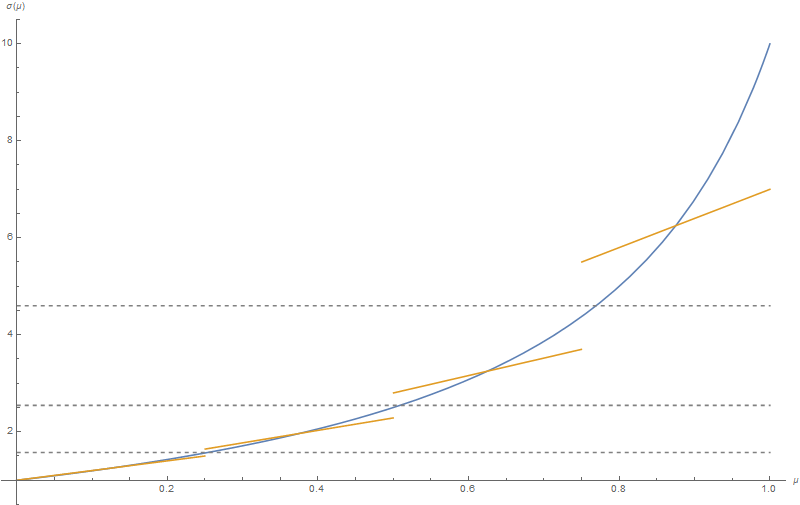
(a) Increasing NE and ABEE functions
with $A=1$,$B=1$ and $C=0.8$

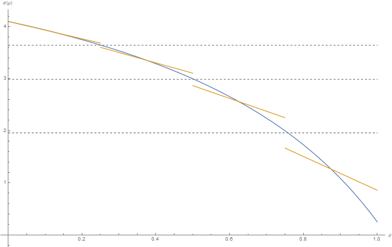
(b) Decreasing NE and ABEE functions
with $A=4.1$,$B=-4$ and $C=0.6$

To present our result, we introduce the notion of equidistant-expectations sequence $\mu_{0},\mu_{1},\dots,\mu_{K}$ defined so that for any $\mu_{k}$, with $k\neq 0,1$, the Euclidean distance between $\mu_{k}$ and the mean value of $\mu$ in $(\mu_{k-1},\mu_{k}]$ is equal to the Euclidean distance between $\mu_{k}$ and the mean value of $\mu$ in $(\mu_{k},\mu_{k+1}]$. That is, $\mu_{k}-E[\mu|(\mu_{k-1},\mu_{k}]]=E[\mu|(\mu_{k},\mu_{k+1}]]-\mu_{k}$. We refer to the corresponding interval partition $(\alpha_{k})_{k=1}^{K}$ with $\alpha_{k}=(\mu_{k-1},\mu_{k}]$ as the equidistant-expectations partition. We note that when $\mu$ is uniformly distributed on $[0,1]$, the equidistant-expectations sequence is uniquely defined by $\mu_{k}=\frac{k}{K}$. For more general density functions $f$, it is readily verified (by repeated application of the intermediate value theorem) that there always exists at least one equidistant-expectations partition.

Our main result in the strategic complements case is:

Proposition 8

In the environment with strategic complements, consider an equidistant-expectations partition $\left(\mu_{k}^{\ast}\right)_{k=0}^{K}$. There exist $\left\{\underline{\mu}_{k},\overline{\mu}_{k}\right\}_{k=0}^{K}$satisfying $\underline{\mu}_{k}<\mu_{k}^{\ast}<\overline{\mu}_{k}$ such that for any $\left(\mu_{k}\right)_{k=0}^{K}$ satisfying $\mu_{k}\in(\underline{\mu}_{k},\overline{\mu}_{k})$, the analogy partition $An=(\alpha_{k})_{k=1}^{K}$ with $\alpha_{k}=(\mu_{k-1},\mu_{k}]$ together with the corresponding ABEE is a locally clustered ABEE.

The rough intuition for this result can be understood as follows. First, start with an equidistant-expectations partition $\left(\mu_{k}^{\ast}\right)_{k=0}^{K}$. Suppose we were considering games with no interaction term, i.e., such that $C=0$. Then in game $\mu$, players would be picking their dominant strategy $a(\mu)=A+\mu B$ irrespective of the analogy partition, given that players would not care about the action chosen by their opponent. It is readily verified that the local clustering conditions for the points $a(\mu)$ would lead to pick an equidistant-expectations partition in this case. Allowing for non-null interaction parameters $C$ makes the problem of finding a locally clustered ABEE a priori non-trivial due to the endogeneity of the data generated by the ABEE with respect to the chosen analogy classes, as emphasized above. However, what the Proposition implies is that using the same analogy classes as those obtained when $C=0$ can be done to construct a locally clustered ABEE. Intuitively, this is so because the strategic complement aspect makes the points obtained through ABEE in a given class of the equidistant-expectations partition look closer to one another relative to points outside a class, as compared with the case in which $C=0$. As a result, the local clustering conditions which hold for the equidistant-expectation partition when $C=0$ hold a fortiori when $C$ is non-null. Now given the jumps, there is some slack in the conditions for local clustering, thereby ensuring that one can find open intervals for the boundary points $\mu_{k}$ that satisfy the conditions of the Proposition.

Our environment with strategic complements can be viewed as one in which there is an element of self-attraction in the choice of analogy partitions. As can easily be inferred from the above discussion, the larger $C$ is, the more analogy interval analogy partitions can be used to support locally clustered ABEE, i.e., the more partitions are self-attractive. In Jehiel and Weber (2023) (the working paper version), we have characterized more fully the set of locally clustered ABEE confirming that insight, and we have noted that when $C$ is too large the equidistant-expectations partition need not be compatible with the requirement for global clustering.

3.3.2 Strategic Substitutes

We consider now the strategic substitute case, and we assume that $\mu$ is distributed according to a continuous density function $f$ with support $[-1,0]$.

Note that, differently from the strategic complements environment, here the ABEE function $a^{ABEE}(\mu)=A+\sum_{k=1}^{K}1_{\{\mu\in[\mu_{k-1},\mu_{k})\}}\mu\frac{B+AC}{1-CE[\mu|\alpha_{k}]}$ is not monotonic in $\mu$. This is due to the fact that at the discontinuity points the jumps of the function are in the opposite direction with respect to the slope of $a(\mu|\alpha_{k})=A+\mu\frac{B+AC}{1-CE[\mu|\alpha_{k}]}$, and this is a fundamental difference induced by the change from strategic complements to strategic substitutes. This is illustrated in Figure 2.

Figure 2: Local Clustering for $K=4$ and $\mu$-sequence such that $\mu_{k}=\frac{k}{4}$, $k=0,1,\dots,4$.

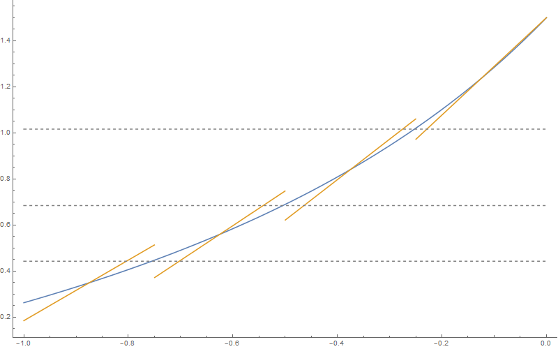
(a) Increasing NE and ABEE functions
with $A=1.5$,$B=1$ and $C=0.9$

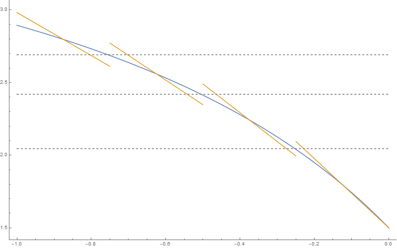
(b) Decreasing NE and ABEE functions
with $A=1.5$,$B=-4$ and $C=0.9$

The non-monotonicities that arise in the ABEE strategies with interval analogy partitions in turn make it impossible to satisfy the local clustering conditions in a neighborhood of $\mu=\mu_{k}$. This is so because it cannot be simultaneously the case that $\lim_{\mu\rightarrow\mu_{k}^{+}}a^{ABEE}(\mu)$ is closer to $\beta((\mu_{k},\mu_{k+1}])$ and $a^{ABEE}(\mu_{k})$ is closer to $\beta((\mu_{k-1},\mu_{k}])$. This simple observation implies:

Proposition 9

In the strategic substitutes environment, whenever $B\neq-AC$, there are no symmetric interval analogy partitions that are locally clustered with respect to the induced ABEE.

Our environment with strategic substitutes illustrates a case with self-repelling analogy partitions. In light of our general theoretical framework, it would then be natural to look for clustered distributional ABEE. In our setting with a continuum of games, this is a challenging task, and in Jehiel and Weber (2023) (the working paper version), we characterize the clustered distributional ABEE when $\mu$ can take only three values.

4 Conclusion

In this paper we have introduced the notion of Clustered ABEE defined so that i) given the analogy partitions, players choose strategies following the ABEE machinery, and ii) given the raw data on the opponent’s strategies, players select analogy partitions so as to minimize the prediction errors (either locally or globally). We have highlighted the existence of environments with self-repelling analogy partitions in which some mixing over analogy partitions must arise as well as environments with self-attractive analogy partitions for which multiple analogy partitions can arise in equilibrium. In the case of environments with self-repelling analogy partitions, an implication of our analysis is that faced with the same objective datasets and the same objective constraints (as measured by the number of classes), players must be processing information in a heterogeneous way in equilibrium. Our derivation of this insight follows from the strategic nature of the interaction, and it should be contrasted with other possible motives of heterogeneity, for example, based on the complexity of processing rich datasets. The case of self-attractive analogy partitions suggests a novel source of multiplicity, not discussed in the previous literature, and it may shed light on why, in such environments, different societies may settle down on different behaviors and different models of expectation formation. Our applications reveal among other things that environments with strategic complements have self-attractive analogy partitions and environments with strategic substitutes have self-repelling analogy partitions.

This study can be viewed as a first step toward a more complete understanding of the structure and impact of categorizations on expectation formation in strategic interactions. Among the many possible future research avenues, one could consider the effect of allowing the clustering to be based not only on the opponent’s distribution of action but also on other characteristics of the interaction such as the own payoff structure. One could also consider the effect of allowing the pool of subjects assigned to the role of a given player to be heterogeneous in the number of categories that can be considered.

Appendix

Proof of Proposition 1

The column player partitions games finely. Let row player’s analogy partition be $An_{1}=\{\{x_{1},x_{2}\},\{x_{3}\}\}$ with $x_{1}<x_{2}$, and let $\beta_{L}$ denote the probability attached to $L$ in the expectation $\beta_{1}(x_{1},x_{2})$.

In any ABEE, the Nash equilibrium strategies are played in $x_{3}$, thus the column player plays $L$ with probability $\frac{1}{2+x_{3}}$ in $x_{3}$ to make the row player indifferent. The row player must be mixing in game $x_{1}$ too: if $\sigma_{1}(x_{1})=D$, then $\sigma_{2}(x_{1})=R$ which implies $\beta_{L}\geq\frac{1}{2}$, while the best response of the row player in $x_{1}$, given $\beta_{L}$, would be $U$; If $\sigma_{1}(x_{1})=U$ is a best response for the row player, it has to be that $\beta_{L}\geq\frac{1}{2+x_{1}}$ which is greater than $\frac{1}{2+x_{2}}$ and so the row player would play $U$ in $x_{2}$ as well. This in turn would imply that column player would play $R$ in both games, which would violate the consistency requirement on $\beta_{L}$.

Therefore, any ABEE requires $\beta_{L}=\frac{1}{2+x_{1}}$. Given $\beta_{L}$, row plays $\sigma_{1}(x_{2})=U$ leading column to play $\sigma_{2}(x_{2})=R$. By consistency, the column player must be playing $L$ with probability $\frac{2}{2+x_{1}}$ in game $x_{1}$.

Note that the strategy profile $\sigma_{2}$ just obtained is such that $An_{1}$ is not locally clustered. If $x_{1}=b$, the probability of playing $L$ in $x_{1}$ is greater than $\frac{1}{2}$, while $\beta_{L}=\frac{1}{2+b}<\frac{1}{2+a}<\frac{1}{2}$, where $\frac{1}{2+a}$ is the probability assigned to $L$ by row’s expectations in $x_{3}=a$: game $x_{1}$ should be reassigned to $x_{3}$. Whenever $x_{1}=a$, regardless of $x_{2}$ being $b$ or $c$, $x_{2}$ should be reassigned to $x_{3}$ because the probability of $L$ being played in $x_{2}$ is zero, which is closer to $\frac{1}{2+x_{3}}$ than to $\beta_{L}=\frac{1}{2+a}$. Q.E.D

Proof of Theorem 1.

Compared to classic existence results in game theory, the main novelty is to show that the global clustering correspondence has properties that allow to apply Kakutani fixed point theorem to a grand mapping $M:\Sigma\times\Lambda\rightrightarrows\Sigma\times\Lambda$, which is a composition of the following functions and correspondences. Given $(\sigma,\lambda)$, we aggregate the strategies following (2) obtaining $\bar{\sigma}$ and we define $\beta$ to be consistent with $\bar{\sigma}$ for all analogy partitions. We denote this function $AG$. We perform global clustering ($GC$) on $(\bar{\sigma},\beta)$ and obtain all $\lambda^{\prime}$ with support only over partitions that are globally clustered with respect to $\bar{\sigma}$. Also, starting from $(\bar{\sigma},\beta)$, the Best Response correspondence ($BR$) yields the optimal strategies for each analogy partition. Then, we obtain the following composition:

$$(\sigma,\lambda)\mapsto_{AG}(\bar{\sigma},\beta)\mapsto_{BR\times GC}(\sigma^{\prime},\lambda^{\prime})$$

here $M(\sigma,\lambda)$ denotes the set of $(\sigma^{\prime},\lambda^{\prime})$ that can be obtained through this composition. That is, $M(\sigma,\lambda)=\{(\sigma^{\prime},\lambda^{\prime})\lvert(\bar{\sigma},\beta)=AG(\sigma,\lambda),\sigma^{\prime}\in BR(\bar{\sigma},\beta),\lambda^{\prime}\in GC(\bar{\sigma},\beta)\}$

Note that $AG$ is a continuous functions, while $BR$ and $GC$ are correspondences. The mapping $BR$ is upper-hemicontinuous (uhc) with non-empty, convex and compact values by standard arguments. Since, as we will prove later, $GC$ is also uhc with non-empty, convex and compact value, it follows that:

(i) $M$ is nonempty;

(ii) $M$ is uhc and compact-valued because the correspondence $BR\times GC$ is uhc and compact-valued as product of uhc and compact-valued mappings (see proposition 11.25 in Border (1985)) and the composition $(BR\times GC\circ AG)(\sigma,\lambda)$ is uhc as composition of uhc mappings (proposition 11.23 in Border (1985)) and compact-valued since $AG$ is single-valued and $BR\times GC$ is compact-valued;

(iii) $M$ is convex-valued since $AG$ is single-valued, while $BR$ and $GC$ are convex-valued. This can be established by noting that $M(\sigma,\lambda)=BR(AG(\sigma,\lambda))\times GC(AG(\sigma,\lambda))$. If $(\sigma^{1},\lambda^{1})$ and $(\sigma^{2},\lambda^{2})$ are both in $M(\sigma,\lambda)$, then for all $\gamma\in[0,1]$, $\gamma\sigma^{1}+(1-\gamma)\sigma^{2}\in BR$ because $BR$ is convex-valued and $\gamma\lambda^{1}+(1-\gamma)\lambda^{2}\in GC$ because $GC$ is convex-valued, thereby implying that $\gamma(\sigma^{1},\lambda^{1})+(1-\gamma)(\sigma^{2},\lambda^{2})\in M(\sigma,\lambda)$. Hence, $M(\sigma,\lambda)$ is convex for all $(\sigma,\lambda)$.

Since $\Sigma\times\Lambda$ is a compact and convex set, properties (i) to (iii) ensure that $M$ has a fixed point by Kakutani’s theorem. A fixed point is a globally CD-ABEE because $GC\circ AG$ ensure globally clustered partitions and $BR\circ AG$ ensure D-ABEE strategies.

To conclude the proof we need to show the properties of the $GC$ correspondence. $GC$ maps $\bar{\Sigma}\times\left((\Delta A_{i})^{K_{i}|\mathcal{K}_{i}|}\times(\Delta A_{j})^{K_{j}|\mathcal{K}_{j}|}\right)$ into $\Lambda$, where all sets are convex and compact. The image $GC(\bar{\sigma},\beta)$ is given by the following set

$$\lambda^{\prime}\in\{\lambda\in\Lambda|\lambda_{i}(An_{i})>0\implies An_{i}\in\arg\min_{An_{i}^{\prime}\in\mathcal{K}_{i}}V(\bar{\sigma}_{j},\beta_{i}^{\prime})\}$$

where $V_{i}(\bar{\sigma}_{j},\beta_{i}^{\prime})=\sum_{\alpha_{i}\in An_{i}^{\prime}}p(\alpha_{i})\sum_{\omega\in\alpha_{i}}p(\omega|\alpha_{i})d\left(\bar{\sigma}_{j}(\omega),\beta_{i}(\alpha_{i}|An_{i}^{\prime})\right)$.

The latter set can be decomposed in $G_{i}(\bar{\sigma}_{j})$ and $G_{j}(\bar{\sigma}_{i})$. Note that $G_{i}$ is nonempty because $\mathcal{K}_{i}$ is finite. Also, $G_{i}$ is a simplex hence it is convex and compact. Thus, $GC$ is nonempty, convex and compact valued. We check that $GC(\bar{\sigma},\beta)$ is uhc by showing that it has a closed graph.

We first establish the continuity of $V_{i}$ by verifying that $d$ is a continuous function. When $d$ is the squared Euclidean distance, $d$ is clearly continuous in $\bar{\sigma}$ and in $\beta$. Instead, when $d$ represents the KL divergence, it is not generally continuous because whenever there is $\omega\in\alpha_{i}$ such that $supp[\bar{\sigma}_{j}(\omega)]\not\subset supp[\beta_{i}(\alpha_{i}|An_{i})]$, then $d(\bar{\sigma}_{j},\beta_{i})$ goes to infinity. However, the consistency requirements impose $supp[\bar{\sigma}_{j}(\omega)]\subseteq supp[\beta_{i}(\alpha_{i}|An_{i})]$. Since global clustering imposes for both players that $\beta_{i}$ is consistent with $\bar{\sigma}_{j}$, for all $\omega,\,\alpha_{i}$ and $An_{i}$, then $d(\bar{\sigma}_{j},\beta_{i})$ is finite. Recall that, $d(x,y)=\sum_{a}(x_{a}\ln x_{a}-x_{a}\ln y_{a})$. Since $x_{a},y_{a}\in[0,1]$ and $x_{a}>0$ implies $y_{a}>0$, under the convention that $0\ln 0=0$, $d$ is continuous when it represents the KL divergence. Hence, $V_{i}$ is continuous, if $\beta_{i}$ is consistent with $\bar{\sigma}_{j}$ for both players.

We can now proceed to establish that $GC$ is uhc. Assume by contradiction that $GC$ does not have a closed graph. That is, $\bar{\sigma}_{j}^{n}\rightarrow\bar{\sigma}_{j}$, $\lambda_{i}^{n}\rightarrow\lambda_{i}$ and $\lambda_{i}^{n}\in G_{i}(\bar{\sigma}_{j}^{n})$, but $\lambda_{i}\notin G_{i}(\bar{\sigma}_{j})$. Note that $\lambda_{i}\notin G_{i}(\bar{\sigma}_{j})$ implies that there is some $\tilde{An}_{i}\in supp[\lambda_{i}]$ and $\varepsilon^{\prime},\varepsilon>0$ such that

$$+\infty>V_{i}(\bar{\sigma}_{j},\tilde{\beta}_{i})\geq V_{i}(\bar{\sigma}_{j},\beta_{i})+\varepsilon+\varepsilon^{\prime}\text{,}$$

where $\tilde{\beta}_{i}$ is consistent with $\bar{\sigma}_{j}$ according to $\tilde{An}_{i}$. Also, let $\tilde{\beta}_{i}^{n}$ be consistent with $\bar{\sigma}_{j}^{n}$, according to $\tilde{An}_{i}$. We want to show that for some $n$, $\lambda_{i}^{n}(\tilde{An}_{i})>0$ and $V_{i}(\bar{\sigma}_{j}^{n},\tilde{\beta}_{i}^{n})>V_{i}(\bar{\sigma}_{j}^{n},\beta_{i}^{n})$. For $\lambda_{i}^{n}\rightarrow\lambda_{i}$ and $\lambda_{i}(\tilde{An}_{i})>0$, for any $n$ large enough, $\lambda_{i}^{n}(\tilde{An}_{i})>0$. As $\bar{\sigma}_{j}^{n}\rightarrow\bar{\sigma}_{j}$, for $n$ large enough, by continuity of $V_{i}$, $V_{i}(\bar{\sigma}_{j}^{n},\beta_{i}^{n})$ is in a neighborhood of $V_{i}(\bar{\sigma}_{j},\beta_{i})$ so we can write: $V_{i}(\bar{\sigma}_{j},\beta_{i})>V_{i}(\bar{\sigma}_{j}^{n},\beta_{i}^{n})-\varepsilon$. Then, $V_{i}(\bar{\sigma}_{j},\tilde{\beta}_{i})\geq V_{i}(\bar{\sigma}_{j},\beta_{i})+\varepsilon+\varepsilon^{\prime}>V_{i}(\bar{\sigma}_{j}^{n},\beta_{i}^{n})+\varepsilon^{\prime}$. Similarly, $\bar{\sigma}_{j}^{n}\rightarrow\bar{\sigma}_{j}$ implies that, for any $n$ large enough, $V_{i}(\bar{\sigma}_{j}^{n},\tilde{\beta}_{i}^{n})>V_{i}(\bar{\sigma}_{j},\tilde{\beta}_{i})-\varepsilon^{\prime}$. Thus,

$$V_{i}(\bar{\sigma}_{j}^{n},\tilde{\beta}_{i}^{n})>V_{i}(\bar{\sigma}_{j},\tilde{\beta}_{i})-\varepsilon^{\prime}\geq V_{i}(\bar{\sigma}_{j},\beta_{i})+\varepsilon>V_{i}(\bar{\sigma}_{j}^{n},\beta_{i}^{n})$$

We get $V_{i}(\bar{\sigma}_{j}^{n},\tilde{\beta}_{i}^{n})>V_{i}(\bar{\sigma}_{j}^{n},\beta_{i}^{n})$ and $\lambda_{i}^{n}(\tilde{An}_{i})>0$, which contradicts $\lambda_{i}^{n}\in G_{i}(\bar{\sigma}_{j}^{n})$. It follows that $GC$ is uhc. Q.E.D.

Proof of Propositions 8

Consider the increasing sequence $\{\mu_{k}\}_{k=0}^{K}$ with $\mu_{0}=0$, $\mu_{k}=\frac{E[\mu|(\mu_{k-1},\mu_{k}]]+E[\mu|(\mu_{k},\mu_{k+1}]]}{2}$, and $\mu_{K}=1$. We check that the sequence we propose satisfies the conditions for local clustering.

That is, $An$ is locally clustered if, for all $k=1,\dots,K-1$, (i) $\left(\beta(\alpha_{k})-a(\mu_{k}|\alpha_{k})\right)^{2}\leq\left(\beta(\alpha_{k+1})-a(\mu_{k}|\alpha_{k})\right)^{2}$, and (ii) $\left(\beta(\alpha_{k+1})-a(\mu_{k}|\alpha_{k+1})\right)^{2}\leq\left(\beta(\alpha_{k})-a(\mu_{k}|\alpha_{k+1})\right)^{2}$.

It is readily verified that condition (i) reduces to $E[\mu|(\mu_{k},\mu_{k+1}]]\geq\frac{2\mu_{k}-E[\mu|(\mu_{k-1},\mu_{k}]]}{1+2C(\mu_{k}-E[\mu|(\mu_{k-1},\mu_{k}]])}$. By substituting $\mu_{k}$ in the inequality with $\frac{E[\mu|(\mu_{k-1},\mu_{k}]]+E[\mu|(\mu_{k},\mu_{k+1}]]}{2}$ we obtain:

$$E[\mu|(\mu_{k},\mu_{k+1}]]>\frac{E[\mu|(\mu_{k},\mu_{k+1}]]}{1+2CE[\mu|(\mu_{k},\mu_{k+1}]]}$$

which is true because the denominator is greater than 1.

Condition (ii) is equivalent to requiring that, if $E[\mu|(\mu_{k-1},\mu_{k}]]<\frac{1}{2C}$, the following inequality holds: $E[\mu|(\mu_{k},\mu_{k+1}]]\leq\mu_{k}+\frac{\mu_{k}-E[\mu|(\mu_{k-1},\mu_{k}]]}{1-2CE[\mu|(\mu_{k-1},\mu_{k}]]}$. Recalling that $\mu_{k}=\frac{E[\mu|(\mu_{k-1},\mu_{k}]]+E[\mu|(\mu_{k},\mu_{k+1}]]}{2}$, we obtain

$$\frac{E[\mu|(\mu_{k},\mu_{k+1}]]-E[\mu|(\mu_{k-1},\mu_{k}]]}{2}<\frac{\frac{E[\mu|(\mu_{k},\mu_{k+1}]]-E[\mu|(\mu_{k-1},\mu_{k}]]}{2}}{1-2CE[\mu|(\mu_{k-1},\mu_{k}]]}$$

which holds because $0<1-2CE[\mu|(\mu_{k-1},\mu_{k}]]<1$ when $E[\mu|(\mu_{k-1},\mu_{k}]]<\frac{1}{2C}$.

Since both conditions hold strictly, sequences in the neighborhood of $\{\mu_{k}\}_{k=0}^{K}$ would also satisfy the conditions for local clustering. Q.E.D.

For Online Publication

Online Appendix A: Learning model 1 (Raw data and Machine Learning)

In this part of the appendix we formalize the first model of learning environment introduced in section 2.6.

Learning dynamics.

There is a continuum of mass 1 of subjects assigned to the role of player $i=1,2$.

We introduce two perturbations that are used to deal with possible indifferences. First, when playing a game, we assume the payoffs are slightly perturbed (see Fudenberg and Kreps (1993) or Esponda and Pouzo (2016)). Specifically, let $\widetilde{\rho}_{i}$ be a random variable with a continuous density $g_{i}$ on $\left[0,1\right]$ and $\varepsilon>0$ a number that should be thought of as small ($\varepsilon$ measures the degree of perturbation)and we assume that the distribution of realizations in the population matches the densities and probabilities induced by $p$ and $\widetilde{\rho}_{i}$. Player $i$ in game $\omega$ (with draws $\rho_{i}(a_{i},\omega),\rho_{i}(a_{i}^{\prime},\omega)$) picks action $a_{i}$ whenever for all $a_{i}^{\prime}\neq a_{i}$,

$$u_{i}(a_{i},\beta_{i},\omega)+\varepsilon\rho_{i}(a_{i},\omega)>u_{i}(a_{i}^{\prime},\beta_{i},\omega)+\varepsilon\rho_{i}(a_{i}^{\prime},\omega)$$

where $\beta_{i}$ refers to player $i$’s expectation about player $j$’s behavior in $\omega$.

The second perturbation concerns how clustering is implemented. Suppose in the previous period $\overline{\sigma}_{j}(\omega)$ represents the aggregate play of population $j$ when playing game $\omega$. Let $\widetilde{\eta}_{i}$ be a random vector with continuous density $h_{i}$ over the interior of $\Delta A_{j}$. We assume that a given player of population $i$ implements a (global) clustering into $K_{i}$ classes of $\left(\overline{s}_{j}(\omega)\equiv\frac{\overline{\sigma}_{j}(\omega)+\varepsilon\eta_{i}(\omega)}{1+\varepsilon}\right)_{\omega\in\Omega}$ where $\eta_{i}(\omega)$ is a realization drawn from $\widetilde{\eta}_{i}$ and the draws are assumed to be independent across games $\omega$. As before, we assume that the distributions of realizations in the population match the density $\widetilde{\eta}_{i}$. To be more specific, player $i$ (with draws $\eta_{i}(\omega)$) picks the partitioning into $K_{i}$ classes so as to solve

$$\arg\min_{P_{i}\in\mathcal{K}_{i}}{\displaystyle\sum_{c_{i}\in P_{i}}}p(c_{i}){\displaystyle\sum_{\omega\in c_{i}}}p(\omega\mid c_{i})d(\overline{s}_{j}(\omega),\beta_{i}(c_{i})),$$

note that in cluster $c_{i}$, the belief $\beta_{i}$ is identified with the mean of $\overline{s}_{j}(\omega)$ conditional on $\omega\in c_{i}$.

The learning dynamics is as described in the main text and it is fully pinned down by the initial values of $\overline{\sigma}^{0}(\omega)$ used in period 1 (as well as $\varepsilon$, $g_{i}$, $h_{i}$).

Steady state.

In this part, we show that for a fixed $\varepsilon$, there always exists a steady state of the learning dynamics just described. We then show that the limits of such steady states as $\varepsilon$ converges to $0$ correspond to the globally clustered distributional ABEE.

Proposition 10

For a fixed $\varepsilon$, there always exists a steady state of the learning dynamics.

Proof. The proof shares similarities with the purification techniques introduced by Harsanyi (1973). We consider the same grand mapping $M$ that we introduced in the proof of Theorem 1, but now in the perturbed environment. The perturbations of the payoffs make best-responses single-valued as commonly observed in the previous learning literature. The main novelty here is that the perturbations on the strategies at the clustering stage make the clustering mapping single-valued too. The argument to show this is a bit more involved than for the payoff perturbation part because the perturbations at the clustering stage do not allow for additive separability.

More precisely, consider the compound mapping $(\bar{\sigma},\lambda)\mapsto_{C}(\beta,\lambda)\mapsto_{BR}(\sigma^{\prime},\lambda)\mapsto_{AG}(\bar{\sigma}^{\prime},\lambda)$ where $\bar{\sigma}^{\prime}$ is the profile of aggregate best-responses, given $\lambda$.

Fix the probability distributions over analogy partitions $\lambda$. From the profile of aggregate strategies $\bar{\sigma}=(\bar{\sigma}_{1},\bar{\sigma}_{2})$ we can compute the corresponding analogy-based expectations $(\beta_{i}(\cdot|An_{i}))_{An_{i}\in supp\lambda_{i}}$ that are consistent with $\bar{\sigma}$. The mapping $(\bar{\sigma},\lambda)\mapsto(\beta,\lambda)$ is continuous, single-valued and defined over convex and compact sets.

We consider best-responses in the perturbed environment. Let us order the actions in $A_{i}$, so that $a_{i}^{z}$ is the $z$-th element in $A_{i}$. We denote by $a_{i}^{\ast}(\omega|An_{i})(\cdot)$ the function that maps each realization of the profile of random variables $\tilde{\rho_{i}}$ for each action $a_{i}\in A_{i}$ in game $\omega$ into a best-response, and we write $a_{i}=a_{i}^{\ast}(\omega|An_{i})(\rho_{i})$ to indicate that $a_{i}$ is played when the profile of realizations is $\rho_{i}(\omega)=(\rho_{i}(a_{i}^{\prime},\omega))_{a_{i}^{\prime}}$ where $\rho_{i}=(\rho_{i}(\omega))_{\omega}$. We denote by $X_{i}^{z}(a_{i}^{\ast}(\omega|An_{i}))$ the set of perturbations under which the action $a_{i}^{z}$ is chosen according to $a_{i}^{\ast}(\omega|An_{i})$. That is:

$$X_{i}^{z}(a_{i}^{\ast}(\omega|An_{i}))=\{\rho_{i}|a_{i}^{z}=a_{i}^{\ast}(\omega|An_{i})(\rho_{i})\}.$$ (5)

The mixed strategy played by player $i$, under the analogy partition $An_{i}$ in game $\omega$ is induced by $a_{i}^{\ast}(\omega|An_{i})$ if and only if $\sigma_{i}(\omega|An_{i})$ assigns probability $p_{i}(a_{i}^{z};\omega,An_{i})$ to $a_{i}^{z}$ where

$$p_{i}(a_{i}^{z};\omega,An_{i})=\int\dots\int_{\rho_{i}\in X_{i}^{z}(a_{i}^{\ast}(\omega|An_{i}))}d\rho_{i}(a_{i}^{1},\omega)\dots d\rho_{i}(a_{i}^{|A_{i}|},\omega)g_{i}(\rho_{i}(a_{i}^{1},\omega))\dots g_{i}(\rho_{i}(a_{i}^{|A_{i}|},\omega))$$ (6)

and $g_{i}(\rho_{i})$ is the continuously differentiable pdf of $\tilde{\rho_{i}}$.

Consider first the mapping $BR:(\beta,\lambda)\mapsto(\sigma^{\prime},\lambda)$, where $\sigma^{\prime}$ is a profile of mixed strategies that is a best-response to $\beta$. Let $a_{i}^{\ast}(\omega|An_{i})$ prescribe actions that are best responses to $\beta_{i}(\cdot|An_{i})$, given the perturbed payoffs. Then $BR$ is single-valued (because the set of realizations of the perturbations under which there are indifferences has measure zero), and it is readily verified that $BR$ is a continuous function over convex and compact sets.

Consider the $AG$ function, $(\sigma^{\prime},\lambda)\mapsto(\bar{\sigma}^{\prime},\beta^{\prime})$ which aggregates the strategies over games and computes consistent expectations. $AG$ is single-valued and continuous. Thus, the compound mapping $(\bar{\sigma},\lambda)\mapsto_{C}(\beta,\lambda)\mapsto_{BR}(\sigma^{\prime},\lambda)\mapsto_{AG}(\bar{\sigma}^{\prime},\beta^{\prime})$ is also continuous and single valued over convex and compact sets.

For the clustering part, the argument is somewhat similar to the best response part. Consider the clustering mapping $GC:(\bar{\sigma}^{\prime},\beta^{\prime})\mapsto(\bar{\sigma}^{\prime},\lambda^{\prime})$, where $\lambda^{\prime}=(\lambda_{i}^{\prime},\lambda_{j}^{\prime})$ is such that $\lambda_{i}^{\prime}$ solves the global clustering problem for player $i$.

Consider the perturbed strategies $\bar{s}$, where $\bar{s}_{j}(\omega)=\frac{\bar{\sigma}_{j}(\omega)+\varepsilon\eta_{i}(\omega)}{1+\varepsilon}$ and impose that $\beta_{i}$ is consistent with $\bar{s}_{j}$. As established in Theorem 1, for each $\omega\in\alpha$, the function $d(\bar{s}_{j}(\omega),\beta_{i}(\alpha|An_{i}))$ is continuous in $\bar{s}_{j}$.

We define $An_{i}^{\ast}(\eta_{i})$ as the function mapping the realization of the perturbation $\tilde{\eta}_{i}$ to an analogy partition $An_{i}$ that solves the clustering problem. As before, we denote by $X_{i}^{k}(An_{i}^{\ast})=\{\eta_{i}|An_{i}^{k}=An_{i}^{\ast}(\eta_{i})\}$ the set of realizations such that the $k$-th analogy partition is prescribed by $An_{i}^{\ast}$.

The mixture of analogy partitions $\lambda_{i}$ is induced by $An_{i}^{\ast}(\cdot)$ iff $\lambda_{i}$ assigns probability $q(An_{i}^{k})$ to $An_{i}^{k}$ where $q(An_{i}^{k})=\int\dots\int_{\eta_{i}\in X_{i}^{k}(An_{i}^{\ast})}d\eta_{i}(\omega_{1})\dots d\eta_{i}(\omega_{N})h_{i}(\eta_{i}(\omega_{1}))....h_{i}(\eta_{i}(\omega_{N}))$, where $h_{i}$ is the continuously differentiable pdf of $\eta_{i}$. We show now that the clustering mapping is single-valued. To establish this, we rely on results from chapter 2 in Milnor (1965). More precisely, we show that if $An_{i}$ and $An_{i}^{\prime}$ yield the same $V$ value (the criterion used for the clustering problem), then the set of realizations of $\tilde{\eta_{i}}$ that allow this has measure zero. Given, $\bar{\sigma}_{j}$ we can define the function $h(\eta_{i})=V_{i}(\bar{s}_{j},\beta_{i}(\cdot|An_{i}))-V_{i}(\bar{s}_{j},\beta_{i}(\cdot|An_{i}^{\prime}))$, which is a mapping $h:U\rightarrow R$, where $\eta_{i}\in U$. The function $h$ is smooth (all partial derivatives exist and are continuous). Since $\eta_{i}(a_{i},\omega)>0$, for all $\omega$ and all $a_{i}$, then $U$ is an open set. As $h(\eta_{i})=0$ is a regular value, then the set $\{\hat{\eta}_{i}|h(\hat{\eta}_{i})=0\}$ is a smooth manifold of dimension $dim(U)-1=(|A_{i}|-1)\cdot|\Omega|-1$, which has measure zero in $U$. Then, the argument for $C$ being single valued and continuous are the same as those used for $BR$.

Thus, the compound mapping

$$M:(\bar{\sigma},\lambda)\mapsto_{C}(\beta,\lambda)\mapsto_{BR}(\sigma^{\prime},\lambda)\mapsto_{AG}(\bar{\sigma}^{\prime},\beta^{\prime})\mapsto_{GC}(\bar{\sigma}^{\prime},\lambda^{\prime})$$

is single-valued and continuous, and it maps $\bar{\Sigma}\times\Lambda$ into $\bar{\Sigma}\times\Lambda$, which are convex and compact sets. By Brouwer’s fixed point theorem, this mapping has a fixed point.

It is then readily verified that the fixed point $(\sigma,\lambda)$ is a steady state of the learning dynamics. Q.E.D.

Proposition 11

Consider a sequence of steady states $(\sigma^{(\varepsilon)},\lambda^{(\varepsilon)})$ of the learning dynamics induced by $\varepsilon$ where $\sigma^{(\varepsilon)}$ denotes the ex ante strategy (prior to the realizations of the perturbations $\rho$) and $\lambda^{(\varepsilon)}$ denotes the distribution of the profile of analogy partitions. Consider an accumulation point $(\sigma,\lambda)$ of $(\sigma^{(\varepsilon)},\lambda^{(\varepsilon)})$ as $\varepsilon$ tends to $0$. $(\sigma,\lambda)$ is a globally clustered distributional ABEE.

Proof. If $\lim_{\varepsilon\rightarrow 0}(\sigma^{(\varepsilon)},\lambda^{(\varepsilon)})=(\sigma,\lambda)$, then for $\varepsilon$ small enough $supp[\sigma_{i}(\omega)]\subseteq supp[\sigma_{i}^{(\varepsilon)}(\omega)]$ and $supp[\lambda_{i}]\subseteq supp[\lambda_{i}^{(\varepsilon)}]$, for $i=1,2$ and $\omega\in\Omega$.

Since $(\sigma^{(\varepsilon)},\lambda^{(\varepsilon)})$ is a steady state, any $An_{i}\in supp[\lambda_{i}^{(\varepsilon)}]$ solves the clustering problem for player $i$ in the perturbed environment. Thus, for $\varepsilon=0$, $An_{i}\in supp[\lambda_{i}]$ solves the clustering problem because $d$ is continuous in $\varepsilon$ (as established in Theorem 1, imposing consistency on $\beta$ suffices to guarantee continuity in the case of KL divergence). The same argument can be made to show that $\sigma$ is a best-response to $\lambda$. Thus, $(\sigma,\lambda)$ is a steady state of the learning dynamics when $\varepsilon=0$.

It follows that $(\sigma,\lambda)$ is a globally clustered ABEE because the requirements for the equilibrium and the steady states coincide when $\varepsilon=0$ and the independence of the random draws ensures that $\sigma\in\Sigma_{1}\times\Sigma_{2}$ and $\lambda\in\Delta\mathcal{K}_{1}\times\Delta\mathcal{K}_{2}$. Q.E.D.

Online Appendix B

Globally CD-ABEE in Example 1

We also provide a description of the globally clustered distributional ABEE.

Let $An_{x}=\{\{x\},\{x^{\prime},x^{\prime\prime}\}\}$ denote an analogy partition of player 1 and $\lambda_{x}=Pr(An_{x})$. Let $p_{x}$ denote the probability that $L$ is played in game $x$ by player 2.

Let $p_{x}\leq p_{x^{\prime}}\leq p_{x^{\prime\prime}}$. For the purposes of global clustering it must be the case that $p_{x^{\prime}}=\frac{p_{x}+p_{x^{\prime\prime}}}{2}$, and also $\lambda_{x^{\prime}}=0$ unless $p_{x}=p_{x^{\prime}}=p_{x^{\prime\prime}}$, but it is readily verified that there is no ABEE such that $p_{x}=p_{x^{\prime}}=p_{x^{\prime\prime}}$.

Then, in order to ensure global clustering, player 2’s strategies must be such that $p_{x}<p_{x^{\prime}}=\frac{p_{x}+p_{x^{\prime\prime}}}{2}<p_{x^{\prime\prime}}$. It is easily verified that there is no distributional ABEE where player 2 is playing pure strategies in game $x$ or $x^{\prime\prime}$. Thus, player 2 is mixing in both games and, clearly, also in $x^{\prime}$. For player 2’s indifference, the aggregate strategy of player 1 $\bar{\sigma}_{1}(x)$ must be to play $U$ with probability $\frac{1}{2}$ in all games $x$. In order to sustain such aggregate strategies for player 1, whenever $x<x^{\prime}<x^{\prime\prime}$ player 1 must be indifferent in game $x^{\prime\prime}$ when using $An_{x}$ and in game $x$ when using $An_{x^{\prime\prime}}$.

To illustrate this, take $x<x^{\prime}<x^{\prime\prime}$. Player 1 expects $L$ to be played with probability $\frac{p_{x}+3p_{x^{\prime\prime}}}{4}$ in games $\{x^{\prime},x^{\prime\prime}\}$ when using $An_{x}$, and with probability $\frac{3p_{x}+p_{x^{\prime\prime}}}{4}$ in games $\{x,x^{\prime}\}$ when using $An_{x^{\prime\prime}}$. By setting the former probability equal to $\frac{1}{2+x}$ and the latter equal to $\frac{1}{2+x^{\prime\prime}}$, we can always sustain $\bar{\sigma}_{1}(x)$ and $\bar{\sigma}_{1}(x^{\prime\prime})$ where $U$ is played with probability $\frac{1}{2}$. Also, since $\frac{p_{x}+3p_{x^{\prime\prime}}}{4}<\frac{1}{2+x^{\prime}}<\frac{3p_{x}+p_{x^{\prime\prime}}}{4}$, player 1 plays $U$ in $x^{\prime}$ when using $An_{x}$ and $D$ when using $An_{x^{\prime\prime}}$. Therefore, $U$ is played in aggregate in $x^{\prime}$ with probability $\frac{1}{2}$ if and only if $\lambda_{x}=\lambda_{x^{\prime\prime}}=\frac{1}{2}$.

ABEE in Beauty-Contest game, section 3.1

We provide here the details needed to compute the ABEE in the framework introduced in section 3.1, in the context of the Beauty-Contest game illustration. We assume players use the same analogy partition $(\Theta_{k})_{k=1}^{K}$. For $\theta\in\Theta_{k}$, player $i$’s best response is: $a_{i}(\theta)=(1-r)\theta+rE[a_{j}(\theta)|\Theta_{k}]$.

Then, the average best response of $i$ in $\theta$ is:

$$E[a_{i}(\theta)|\Theta_{k}]=\int_{\Theta_{k}}a_{i}(\theta)f(\theta|\Theta_{k})d(\theta)=(1-r)E[\theta|\Theta_{k}]+rE[a_{j}(\theta)|\Theta_{k}]\iff$$

$$E[a_{i}(\theta)|\Theta_{k}]=(1-r)E[\theta|\Theta_{k}]+r\left((1-r)E[\theta|\Theta_{k}]+rE[a_{i}(\theta)|\Theta_{k}]\right)$$

and so both players expects their opponent to play the average $\theta$ in the analogy class: $E[a_{1}(\theta)|\Theta_{k}]=E[a_{2}(\theta)|\Theta_{k}]=E[\theta|\Theta_{k}]$ and they play:

$$a_{1}^{ABEE}(\theta)=a_{2}^{ABEE}(\theta)=(1-r)\theta+rE[\theta|\Theta_{k}]$$

Proof of Proposition 7.

By definition, $\sigma_{j}(\mu)\in BR_{j}(\mu,\beta_{i}(\alpha_{k}))$ implies that the following equations must hold in equilibrium:

$$\sigma_{j}(\mu)=A+\mu B+\mu C\int_{\mu_{k-1}}^{\mu_{k}}\frac{f(\mu)}{F(\mu_{k})-F(\mu_{k-1})}\sigma_{i}(\mu)d\mu\hskip 128.0374pt$$

$$=A+\mu\left(B+AC+BC\,E[\mu|\alpha_{k}]+C^{2}E[\mu|\alpha_{k}]\int_{\mu_{k-1}}^{\mu_{k}}\frac{f(\nu)}{F(\mu_{k})-F(\mu_{k-1})}\sigma_{j}(\nu)d\nu\right)$$

Taking the weighted average of $\sigma_{j}(\mu)$ over the interval $[\mu_{k-1},\mu_{k}]$, according to the distribution of $\mu$, yields the following equation:

$$\int_{\mu_{k-1}}^{\mu_{k}}\frac{f(\mu)}{F(\mu_{k})-F(\mu_{k-1})}\sigma_{j}(\mu)d\mu=$$

$$=A+E[\mu|\alpha_{k}]\left(B+AC+BC\,E[\mu|\alpha_{k}]+C^{2}E[\mu|\alpha_{k}]\int_{\mu_{k-1}}^{\mu_{k}}\frac{f(\nu)}{F(\mu_{k})-F(\mu_{k-1})}\sigma_{j}(\nu)d\nu\right)$$

By consistency of $\beta_{i}(\alpha_{k})$, the equation above simplifies into $\beta_{i}(\alpha_{k})=\frac{A+B\,E[\mu|\alpha_{k}]}{1-C\,E[\mu|\alpha_{k}]}$.

In equilibrium, both players have the same expectations $\beta_{1}(\alpha_{k})=\beta_{2}(\alpha_{k})$. Substituting the expression of $\beta_{i}(\alpha_{k})$ into the best-responses yields the following equilibrium (pure) strategies: for all $\alpha_{k}\in An_{1}$ (and $An_{2}$) and for all $\mu\in\alpha_{k}$,

$$\sigma_{1}(\mu)=\sigma_{2}(\mu)=A+\mu\frac{B+AC}{1-C\,E[\mu|\alpha_{k}]}$$

This is the unique ABEE and it is symmetric. Q.E.D.

Lemma 1

Let $\sigma$ be some strategy profile and $d$ be either the squared Euclidean distance or the KL divergence. If $An_{i}\in\mathcal{K}_{i}$ is a globally clustered analogy partition for player $i$ with respect to $\sigma$, then $An_{i}$ is a locally clustered analogy partition for player $i$ with respect to $\sigma$.

Proof. Let $An_{i}$ be a globally clustered analogy partition with respect to $\sigma$. Let $\beta_{i}$ be consistent with $\sigma$. Assume by contradiction that $An_{i}$ is not locally clustered. Then, $\exists\alpha_{i},\alpha\prime_{i}\in An_{i}\,\wedge\,\hat{\omega}\in\alpha_{i}$ s.t. $d(\sigma_{j}(\hat{\omega}),\beta_{i}(\alpha_{i}))>d(\sigma_{j}(\hat{\omega}),\beta_{i}(\alpha\prime_{i}))$.
Let $\widehat{\alpha}_{i}=\alpha_{i}\setminus\{\hat{\omega}\}$ and $\widehat{\alpha\prime}_{i}=\alpha\prime_{i}\cup\{\hat{\omega}\}$. Then,

$$\sum_{\omega\in\alpha_{i}}p(\omega)d(\sigma_{j}(\omega),\beta_{i}(\alpha_{i}))+\sum_{\omega\in\alpha\prime_{i}}p(\omega)d(\sigma_{j}(\omega),\beta_{i}(\alpha\prime_{i}))$$

$$>\sum_{\omega\in\widehat{\alpha_{i}}}p(\omega)d(\sigma_{j}(\omega),\beta_{i}(\alpha_{i}))+\sum_{\omega\in\widehat{\alpha\prime_{i}}}p(\omega)d(\sigma_{j}(\omega),\beta_{i}(\alpha\prime_{i}))$$

$$=p(\widehat{\alpha_{i}})\sum_{\omega\in\widehat{\alpha_{i}}}p(\omega|\widehat{\alpha_{i}})d(\sigma_{j}(\omega),\beta_{i}(\alpha_{i}))+p(\widehat{\alpha\prime_{i}})\sum_{\omega\in\widehat{\alpha\prime_{i}}}p(\omega|\widehat{\alpha\prime_{i}})d(\sigma_{j}(\omega),\beta_{i}(\alpha\prime_{i}))$$

$$>p(\widehat{\alpha_{i}})\sum_{\omega\in\widehat{\alpha_{i}}}p(\omega|\widehat{\alpha_{i}})d(\sigma_{j}(\omega),\beta_{i}(\widehat{\alpha_{i}}))+p(\widehat{\alpha\prime_{i}})\sum_{\omega\in\widehat{\alpha\prime_{i}}}p(\omega|\widehat{\alpha\prime_{i}})d(\sigma_{j}(\omega),\beta_{i}(\widehat{\alpha\prime_{i}}))$$

where the second inequality holds because, when $\beta_{i}$ is consistent with the strategies played in the games in a given analogy class, this is the representative object that minimizes the sum of prediction errors in that analogy class among all possible representative objects in $\Delta A_{j}$.

Let $\widehat{An}_{i}=\widehat{\alpha}_{i}\cup\widehat{\alpha\prime}_{i}\cup\{An_{i}\setminus\{\alpha_{i},\alpha\prime_{i}\}\}$, then:

$$\sum_{\alpha_{i}\in An_{i}}p(\alpha_{i})\sum_{\omega\in\alpha_{i}}p(\omega|\alpha)d(\sigma_{j}(\omega),\beta_{i}(\alpha_{i}))>\sum_{\alpha_{i}\in\widehat{An}_{i}}p(\alpha_{i})\sum_{\omega\in\alpha_{i}}p(\omega|\alpha_{i})d(\sigma_{j}(\omega),\beta_{i}(\alpha_{i}))$$

which contradicts $An_{i}$ being a globally clustered analogy partition. Q.E.D.

Lemma 2

(Reverse Truncation) Let $X$ be a RV on $[0,1]$ with continuous pdf $f_{X}$ and cdf $F_{X}$. There exists a continuous pdf $g$ over $[0,+\infty)$, such that:

$$g_{X|[0,1]}(x)=f_{X}(x),\,\text{where}\,\,\,g_{X|[0,1]}(x)=\frac{g_{X}(x)}{Pr_{g}[0\leq X\leq 1]}$$

Proof. We want to find a continuous function $g_{X}$ such that:

$$g_{X}(x)=\begin{cases}Pr_{g}[0\leq X\leq 1]f_{X}(x)&0\leq x\leq 1\\ v(x)&1<x<\infty\end{cases}$$

Note that $g_{X}$ is continuous if $v(\cdot)$ is continuous and $v(1)=Pr_{g}[0\leq X\leq 1]f_{X}(1)$. Also, $g_{X}$ must be a pdf, so it must be the case that $\int_{0}^{+\infty}g_{X}(x)dx=1$. That is, $\int_{0}^{1}Pr_{g}[0\leq X\leq 1]f_{X}(x)dx+\int_{1}^{+\infty}v(x)dx=Pr_{g}[0\leq X\leq 1]+(1-Pr_{g}[0\leq X\leq 1])=1$.

Let us pick the right function $v(.)$. This function must be continuous and satisfy two conditions: (i) $\int_{1}^{+\infty}v(x)dx=1-T$, and (ii) $v(1)=Tf_{X}(1)$, where $T\equiv Pr_{g}[0\leq X\leq 1]$. Let $v()$ be defined as $v(x)=Tf(1)e^{\frac{Tf(1)}{1-T}(1-x)}$ which is continuous since, for $a,b\in\mathbb{R}$, the function $ae^{bx}$ is continuous in $x$. Also, $v(1)=Tf(1)e^{\frac{Tf(1)}{1-T}(0)}=Tf(1)$.

And finally: $\int_{1}^{+\infty}v(x)dx=Tf(1)e^{\frac{Tf(1)}{1-T}}\int_{1}^{+\infty}e^{-\frac{Tf(1)}{1-T}x}dx=1-T$. Q.E.D.

Lemma 3

There always exists an equidistant-expectations partition.

Proof. We show that there always exists a sequence $\{\mu_{k}\}_{k=0}^{k}$ with $\mu_{0}=0$, some $\mu_{1}\in[0,1]$ and, for $k=2,\dots,K$, $\mu_{k}$ defined so that $\mathbb{E}[\mu|(\mu_{k-1},\mu_{k}]]=2\mu_{k-1}-\mathbb{E}[\mu|(\mu_{k-2},\mu_{k-1}]]$. We note that if $\mu_{1}$ is too large, $\mu_{K}$ might be above 1. Lemma 2 allows us to consider $\mu$ to be a random variable from $[0,+\infty)$ distributed according to a continuous strictly positive pdf $g$, and cdf $G$, with $g(\mu)=f(\mu)G(1)$, for $0\leq\mu\leq 1$.

Let $\mu_{k}\geq\mu_{k-1}\geq 0$. Since $g(\mu)$ is strictly positive and continuous in $\mu$, then $\mathbb{E}[\mu|(\mu_{k-1},\mu_{k}]]=\frac{1}{G(\mu_{k})-G(\mu_{k-1})}\int_{\mu_{k-1}}^{\mu_{k}}\mu g(\mu)d\mu$ is continuous and strictly decreasing in $\mu_{k-1}$, and it is continuous and strictly increasing in $\mu_{k}$. Moreover, if $\mu_{k}\leq 1$, we have:

$$\frac{\int_{\mu_{k-1}}^{\mu_{k}}\mu g(\mu)d\mu}{G(\mu_{k})-G(\mu_{k-1})}=\frac{\int_{\mu_{k-1}}^{\mu_{k}}\mu G(1)f(\mu)d\mu}{G(1)(F(\mu_{k})-F(\mu_{k-1}))}$$

so the term $G(1)$ cancels out and we are back to the original distribution $F$.

Fix $\mu_{k-1}$. The function $m(\mu_{k})\equiv\mathbb{E}[\mu|[\mu_{k-1},\mu_{k}]]$ is continuous and strictly increasing over $(\mu_{k-1},+\infty)$, with image $(\mu_{k-1},+\infty)$. Then the inverse function $m^{-1}$ exists over $(\mu_{k-1},+\infty)$ and it is continuous and strictly increasing over $(\mu_{k-1},+\infty)$.

Given $\mu_{k-2},\mu_{k-1}$, we use the inverse function to retrieve $\mu_{k}$ from the equation $\mathbb{E}[\mu|(\mu_{k-1},\mu_{k}]]=2\mu_{k-1}-\mathbb{E}[\mu|(\mu_{k-2},\mu_{k-1}]]$. Let $h(\mu_{k-2},\mu_{k-1})\equiv 2\mu_{k-1}-\mathbb{E}[\mu|(\mu_{k-2},\mu_{k-1}]]$. Note that $h(\cdot)$ is a continuous function and $h(\mu_{k-2},\mu_{k-1})\geq\mu_{k-1}$.

Starting from $\mu_{0}=0$ and some $\mu_{1}(\mu_{1})\equiv\mu_{1}$, we recursively define $\mu_{k}$ as a function of $\mu_{1}$ as follows: $\mu_{2}(\mu_{1})=m^{-1}(h(\mu_{0},\mu_{1}))$ and

$$\mu_{k}(\mu_{1})=m^{-1}(h(\mu_{k-2}(\mu_{1}),\mu_{k-1}(\mu_{1})))$$

for $k=3,\dots,K$. Note that, for each $k$, the function $\mu_{k}(\mu_{1})$ is well defined. Since $h(\mu_{k-2},\mu_{k-1})\geq\mu_{k-1}$, then the inverse function exists at the point $h(\mu_{k-2},\mu_{k-1})$.

Since $m^{-1}:(\mu_{k-1},+\infty)\rightarrow(\mu_{k-1},+\infty)$ is also strictly increasing and continuous, then $\mu_{k}(\mu_{1})$ is continuous, being a composition of continuous functions, and $\mu_{k}(\mu_{1})\geq\mu_{k-1}$, with equality if and only if $h(\mu_{k-2},\mu_{k-1})=\mu_{k-1}\iff\mu_{k-1}=\mathbb{E}[\mu|(\mu_{k-2},\mu_{k-1}]]\iff\mu_{k-1}=\mu_{k-2}$. So, either we get the sequence with 0 everywhere, or a strictly increasing sequence.

Let $\mu_{1}=0$, then $\mu_{K}(0)=0$. Let $\mu_{1}=1$, then $\mu_{K}(1)>1$. Then, by the intermediate value theorem, there must exist $0<\mu_{1}^{\ast}<1$ such that $\mu_{K}=1$. Q.E.D.

References

- [1] Al-Najjar N. and M. Pai (2014): “Coarse Decision Making and Overfitting,” Journal of Economic Theory, 150, 467–86.
- [2] Anderson J. R. (1991): “The adaptive nature of human categorization,” Psychological Review, 98(3), 409–429.
- [3] Aragones E., I. Gilboa, A. Postlewaite and D. Schmeidler (2005): “Fact-Free Learning,” American Economic Review, 95(5), 1355–1368.
- [4] Banerjee A., X. Guo and H. Wang (2005): “On the optimality of conditional expectation as a Bregman predictor”, IEEE Transactions on Information Theory, 51(7), 2664-2669.
- [5] Battigalli P. (1987): “Comportamento razionale ed equilibrio nei giochi e nelle situazioni sociali”, unpublished undergraduate dissertation, Bocconi University, Milano
- [6] Border, K. C. (1985): Fixed point theorems with applications to economics and game theory. Cambridge university press.
- [7] Esponda I. and D. Pouzo (2016): “Berk-Nash Equilibrium: A Framework for Modeling Agents With Misspecified Models,” Econometrica, 84 (3), 1093–1130.
- [8] Eyster E. and M. Rabin (2005): “Cursed Equilibrium,” Econometrica, 73(5), 1623–1672.
- [9] Fryer R. and M. Jackson (2008): “A Categorical Model of Cognition and Biased Decision-Making,” Contributions in Theoretical Economics, 8(1).
- [10] Fudenberg D. and D. Kreps (1993): “Learning Mixed Equilibria,” Games and Economic Behavior, 5 (3), 320–367.
- [11] Fudenberg D. and G. Lanzani (2023): “Which misperceptions persist?,” Theoretical Economics, 18 (3), 1271–1315.
- [12] Fudenberg D., G. Lanzani and P. Strack (2024): “Selective memory equilibrium”, Journal of Political Economy, 132 (12), 3978–4020
- [13] Gibbons R., M. LiCalzi and M. Warglien (2021): “What situation is this? Shared frames and collective performance,” Strategy Science 6 (2), 124–140
- [14] Harsanyi, J. C. (1973): “Games with randomly disturbed payoffs: A new rationale for mixed–strategy equilibrium points.” International journal of game theory, 2(1), 1–23.
- [15] Jakobsen A. M. (2020): “A Model of Complex Contracts.”, American Economic Review, 110 (5): 1243–73.
- [16] Jehiel P. (1995): “Limited horizon forecast in repeated alternate games,” Journal of Economic Theory, 67 (2), 497–519.
- [17] Jehiel P. (2005): “Analogy-based expectation equilibrium,” Journal of Economic Theory 123, 81–104.
- [18] Jehiel P. (2022): “Analogy-based expectation equilibrium and related concepts: Theory, applications, and beyond,” Prepared for the twelfth World Congress of the Econometric Society.
- [19] Jehiel P. and F. Koessler (2008): “Revisiting Bayesian games with analogy-based expectations,” Games and Economic Behavior, 62, 533–557.
- [20] Jehiel P. and E. Mohlin (2023): “Categorization in Games: A Bias-Variance Perspective,” WP ffhalshs04154272f
- [21] Jehiel P. and D. Samet (2007): “Valuation equilibrium,” Theoretical Economics, 2 (2), 163–185.
- [22] Jehiel P. and G. Weber (2023): “Calibrated Clustering and Analogy-Based Expectation Equilibrium,” PSE Working Papers halshs-04154234, HAL.
- [23] Keynes J.M. (1936): ’The General Theory of Employment, Interest and Money, Macmillan, Cambridge University Press.
- [24] Lloyd S.P. (1957): “Least squares quantization in PCM,” Bell Laboratories Technical Memorandum, later published as: Lloyd, S.P. (1982): “Least squares quantization in PCM,” IEEE Transactions on Information Theory, 28(2), 129–137.
- [25] MacQueen J. (1967): “Classification and analysis of multivariate observations,” In 5th Berkeley Symp. Math. Statist. Probability, 281-297.
- [26] Mengel, F. (2012): “Learning Across Games,” Games and Economic Behavior, 74(2), 601–619.
- [27] Medin, D. L. and M. M. Schaffer (1978): “Context theory of classification learning,” Psychological Review, 85(3), 207–238.
- [28] Miller G. A. (1956): “The magical number seven, plus or minus two: Some limits on our capacity for processing information,” Psychological Review, 63(2), 81–97.
- [29] Milnor J. (1965): ’Topology from the Differential Viewpoint’, University Press of Virginia
- [30] Mohlin E. (2014): “Optimal Categorization,” Journal of Economic Theory, 152, 356–381.
- [31] Myerson, R. and P. Reny (2020): “Perfect Conditional -Equilibria of Multi-Stage Games With Infinite Sets of Signals and Actions,” Econometrica, 88 (2), 495–531.
- [32] Neyman A. (1985): “Bounded complexity justifies cooperation in the finitely repeated prisoners’ dilemma”, Economics letters, 19 (3), 227–229
- [33] Nosofsky, R. M. (1986): “Attention, similarity, and the identification-categorization relationship,” Journal of Experimental Psychology: General, 115(1), 39–57.
- [34] Nyarko, Y. (1991): “Learning in mis-specified models and the possibility of cycles,”Journal of Economic Theory,, 55(2), 416–427.
- [35] Osborne M. and A. Rubinstein (1998): “Games with Procedurally Rational Players,” American Economic Review,, 88(4), 834–47.
- [36] Pȩski M. (2011): “Prior symmetry, categorization and similarity-based reasoning,” Journal of Economic Theory, 146(1), 111–140
- [37] Posner, M. I. and S.W. Keele (1968): “On the genesis of abstract ideas,” Journal of Experimental Psychology, 77(3, Pt.1), 353–363.
- [38] Reed, S. K. (1972): “Pattern recognition and categorization,” Cognitive Psychology, 3(3), 382–407.
- [39] Rosch, E. and B.B. Lloyd (Eds.). (1978): Cognition and categorization. Lawrence Erlbaum.
- [40] Rubinstein A. (1986): “Finite automata play the repeated prisoner’s dilemma”, Journal of economic theory, 39 (1), 83-96
- [41] Samuelson, L. (2001). “Analogies, adaptation, and anomalies,” Journal of Economic Theory, 97(2), 320–366.
- [42] Sims C.A. (2003): “Implications of rational inattention,” Journal of Monetary Economics, 50(3), 665–690.
- [43] Spiegler R. (2016): “Bayesian Networks and Boundedly Rational Expectations,” Quarterly Journal of Economics, 131, 1243–1290.
- [44] Steinhaus H. (1957): “Sur la division des corps materiels en parties,” Bulletin L’Academie Polonaise des Science, 4, 801–804.
- [45] Vives X. (1999): Oligopoly pricing: old ideas and new tools, MIT press.