An Attentional Model of Time Discounting

Abstract

When decision makers evaluate a sequence of rewards, they may pay more attention to larger rewards and, given attention is limited, less attention to smaller rewards. They may also become less attentive to each reward when attention is spread over a longer period of time. Such reductions in attention could lead to greater discounting of the rewards’ values. This paper introduces a novel theory of time discounting based on these assumptions. The resulting discount factors in the theory follow a distribution similar to the multinomial logit function. We characterize such discount factors using two approaches: one based on information maximizing exploration and the other based on the optimal discounting framework. The theory can explain a wide range of anomalies, including the hidden-zero effect, S-shaped value function, and intertemporal correlation aversion. Also, it specifies new mediators for some well-known psychological effects, such as the common difference effect, risk aversion over time lotteries, and the present bias.

1 Introduction

In real-world decisions, individuals often need to evaluate sequences of rewards. For example, they may design a consumption plan that allocates their budget across several weeks, choose among subscription plans that deliver varying benefits across months, or compare job offers with different salary trajectories across years. Such problems are commonly modeled using the additive discounted utility framework (see Cohen et al.,, 2020). In classical discounted utility models, such as exponential and hyperbolic discounting, researchers typically assume that a decision-maker (DM) discounts a future reward solely based on its temporal distance. However, a growing body of research suggests that the valuation of a particular reward within a sequence is often shaped by the presence and structure of other rewards in that sequence (Loewenstein and Prelec,, 1993; Urminsky and Kivetz,, 2011; Read and Scholten,, 2012; Scholten and Read,, 2014; Scholten et al.,, 2016). In this paper, we propose that attention can modulate this influence.

Figure 1 includes two subfigures that illustrate properties of attention potentially relevant to this paper. In each subfigure, one can try fixating on the cross. For subfigure (a), the letters on the right are clearly visible. However, because attention is concentrated on the cross, identifying the fifth letter (“N”) could be difficult due to the small volume of attention allocated to it. For subfigure (b), the lines on both sides are easily seen, but it will be harder to distinguish the individual lines from each other on the left side compared to the right side, as on the left side, attention is spread across more stimuli. In each subfigure, stimuli that receive less attention tend to be processed more shallowly.

An additional but noteworthy phenomenon is value-driven attentional capture (Hickey et al.,, 2010; Anderson et al.,, 2011; Chelazzi et al.,, 2013). Specifically, it refers to the finding that, in visual search tasks, stimuli previously associated with high rewards can automatically capture attention, even when they become irrelevant distractors. This attention shift can impair task performance, such as slowing down the speed of search.

(a) an example of selective attention

(b) an example of the crowding effect

Note: Set the document to 100% zoom, keep your eyes approximately 30 cm from the page, and fixate on the cross in each subfigure. In subfigure (a), the letters on the right are clearly visible. However, it may be challenging to identify the fifth letter (“N”), as little attention is directed toward it. In subfigure (b), the lines on both sides are easily seen, but it may be harder to distinguish the individual lines on the left side compared to the right, as attention is distributed across more stimuli on that side.

Figure 1: Illustrative examples about attention

Similar phenomena may also arise when individuals evaluate a sequence of rewards. To illustrate, consider two intuitive examples. Suppose you are offered a sequence in which you receive £30 today and £20 in a month. Now imagine two basic modifications to this sequence. First, suppose the amount of one reward is substantially increased—for instance, the £20 reward is raised to £8,020. When evaluating the new sequence “receive £30 today and £8,020 in a month”, the large future reward may capture most of your attention (analogous to value-driven attentional capture). That is, you may concentrate on the £8,020 reward and care less about the other reward £30 as the latter becomes less important. As a result, the £30 reward may receive shallower processing, leading it to be undervalued relative to its valuation in the original sequence.

Second, suppose that more rewards, delivered at other time periods, are added into the sequence—for instance, the original sequence is changed to “receive £30 today, and £20 in a month, and £10 in two months, and £15 in three months, and £25 in four months”. To evaluate this new sequence, all rewards must be considered. As the number of rewards increases, the sequence becomes more complex, and each individual reward may receive less attention due to limited cognitive resources. Although you may still understand what occurs at each time point, the depth of processing for each reward may diminish, leading to a vaguer or more superficial valuation.

In both cases, reduced attention to the £30 reward may result in greater discounting of its value. We develop a new model of time discounting to capture such intuitions. In the model, the DM’s baseline patience, prior to receiving any information about the reward sequence, is characterized by classical discount factors that depend solely on time. The classical discount factor for period $t$ is denoted by $d_{t}$. When evaluating a reward sequence, these discount factors are influenced by attention mechanisms and altered into decision weights $w_{t}$.

We assume that when evaluating a reward sequence, each reward serves as an independent information source. The DM cannot fully process the information from all rewards simultaneously. Therefore, she selectively attends more to the rewards that will have the largest impact on sequence value: a larger reward should be given a greater decision weight, while a smaller one should be given a smaller decision weight.

Let $s_{0\rightarrow T}=[s_{0},s_{1},…,s_{T}]$ denote a sequence of rewards delivered from period 0 to period $T$, where $s_{t}$ represents the reward in period $t$. Then, this sequence’s value can be represented in a similar way to the additive discounted utility framework, by $U(s_{0\rightarrow T})=\sum_{t=0}^{T}w_{t}u(s_{t})$. The decision weight $w_{t}$ is increasing in the attention allocated to $s_{t}$.

Notably, we recommend using a simple form to specify $w_{t}$:

$$w_{t}=\frac{d_{t}e^{u(s_{t})/\lambda}}{\sum_{\tau=0}^{T}d_{t}e^{u(s_{\tau})/\lambda}}$$

where the parameter $\lambda>0$, and the instantaneous utility $u(s_{t})\geq 0$. This specification of $w_{t}$ takes the multinomial logit (also called softmax) function. In this function, $w_{t}$ is increasing in reward $s_{t}$ but decreasing in other rewards, indicating a tendency to focus on large rewards (which captures the first intuitive example). The total of decision weights is a fixed amount, which indicates the DM’s attention capacity is limited and when she divides attention over more periods, each period would receive less attention (which captures the second intuitive example). The determination of $w_{t}$ is subject to the “original” discount factor $d_{t}$, but also reflects some attentional mechanisms. Thus, we term our model by the attention-modulated discounting (AMD) model.

Our recommended form of $w_{t}$ has three desired features. First, we introduce only one additional parameter $\lambda$ to the standard discounting models. This makes our model not only capable of explaining a range of phenomena, but also highly parsimonious. Meanwhile, the parameter $\lambda$, as we discuss later, is set to decrease in the DM’s cognitive uncertainty as well as the learning rate. This allows researchers to test our model through process-tracing methods.

Second, $w_{t}$ follows a softmax function, which is widely used to model attention in various research areas. In discrete choice research, the softmax function can be used to represent the DM’s choice strategy under attention constraint (Matějka and McKay,, 2015); in memory research, Bordalo et al., (2020) use this function as the attention weight for recalled experiences; in computer science, the softmax function can capture attention to visual cues when processing an image, as well as attention to key words when understanding a text (Xu et al.,, 2015; Vaswani et al.,, 2017). Our model thus has the potential to be integrated with these models to form a unified framework for analyzing the role of attention in decision-making.

Third, $w_{t}$ satisfies a property that we term Sequential Bracket-Independence. To illustrate this property, consider the value representation of a reward sequence $s_{0\rightarrow T}$. We can bracket its first $T$ periods into another sequence $s_{0\rightarrow T-1}=[s_{0},...,s_{T-1}]$. So, the value of $s_{0\rightarrow T}$ can also be represented by a weighted sum of the values of $s_{0\rightarrow T-1}$ and $s_{T}$. That is, $U(s_{0\rightarrow T})=\alpha U(s_{0\rightarrow T-1})+\beta u(s_{T})$ where $\alpha,\beta$ are the decision weights. Sequential Bracket-Independence implies that, the decision weight for any $u(s_{t})$ in the value representation of $s_{0\rightarrow T}$ is independent of whether we conduct this bracketing operation. In this case, we must have $\beta=w_{T}$. Under this property, how the DM values a reward sequence is independent of how she might bracket it. For each particular sequence, there is only one unique distribution of decision weights.

1.1 Two Characterization Approaches

We characterize the AMD model by two approaches. Notably, across various fields including economics, psychology, and machine learning, two typical frameworks are used to model attention (Xu et al.,, 2015; Gabaix,, 2019; Lindsay,, 2020; Loewenstein and Wojtowicz,, 2025). The first assumes that DM operates in an information-rich environment and adjusts the probabilities of sampling information from different sources to achieve certain goals (“hard attention”). The second involves the weighting of different items or attributes when they are integrated into a total representation (“soft attention”). Our first approach reflects the “hard attention” and the second approach reflects the “soft attention”.

The first approach is inspired by reinforcement learning and neuroscientific literature. Our mathematical assumptions are similar to Itti and Baldi, (2009) and Gottlieb et al., (2013). We assume the DM randomly switches attention across different rewards. Each time, she samples a reward and uses the perceived (noisy) value of that reward as a signal for the sequence value. Accordingly, she updates her belief about the sequence value using Bayes’ rule. The objective of sampling is to maximize the information gain, measured by the Kullback–Leibler (KL) divergence of the posterior belief from the prior belief. In other words, the DM’s attention is curiosity-driven: she tends to focus on the reward that brings the greatest surprise compared to her prior belief. In intuition, before the DM starts acquiring any information about the sequence, she should believe it contains no value. So, larger rewards, which deviate more from the zero value, can produce more surprises and thus receive higher decision weights. Specifically, we assume that DM uses the softmax exploration strategy to achieve her objective, as studies have suggested it has strong predictive power for human behavior and neural activities during reinforcement learning (Daw et al.,, 2006; Collins and Frank,, 2014) .

The second approach is an axiomatic analysis. We draw on the optimal discounting framework (Noor and Takeoka,, 2022, 2024) to assume that adjusting $d_{t}$ to $w_{t}$ triggers a cognitive cost, and that the DM’s objective is to maximize the net value of the reward sequence. This assumption implies that DM tends to focus on the information source providing the greatest pleasure. We show that within the optimal discounting framework, the softmax weighting function is the only function that simultaneously satisfies the standard preference axioms, Sequential Bracket-Independence, and Sequential Outcome-Betweenness. We have demonstrated the implication of Sequential Bracket-Independence. Sequential Outcome-Betweenness implies that adding a tiny reward to the end of a reward sequence should result in the sequence being valued lower than the original sequence but higher than that tiny reward alone. This property is critical for explaining some attention-related intertemporal choice anomalies, such as the violation of dominance (Scholten and Read,, 2014; Jiang et al.,, 2017) and the hidden zero effect (Magen et al.,, 2008; Radu et al.,, 2011; Read et al.,, 2017; Dang et al.,, 2021).

1.2 Applications and Related Literature

The AMD model is related to a wide range of decision anomalies. First, the model is consistent with a series of empirical findings, including the hidden zero effect. Suppose a DM is indifferent between “receive £100 today” and “receive £120 in 25 weeks”. The hidden zero effect suggests that, if we frame the former option as “receive £100 today and £0 in 25 weeks”, the DM would become less likely to choose this option. This effect provides a robust technique for altering people’s patience but cannot be explained by standard discounting models. According to our model, the given change extends the sequence length and directs some of the DM’s attention to a future period with no reward delivered, which in turn, reduces the attention for the £100 payment, thereby producing the hidden zero effect.

Second, the model makes novel predictions about some existing findings, such as the common difference effect (Loewenstein and Prelec,, 1992), and risk aversion over time lotteries (Onay and Öncüler,, 2007; DeJarnette et al.,, 2020). For example, it predicts that in comparison between a small sooner reward (SS) and a large later reward (LL), if the difference between reward delays is substantially larger than the difference between reward utilities, the common difference effect may be reversed. That is, adding a common delay to both SS and LL can lead people to exhibit less patience. Besides, it predicts that people are risk averse over time lotteries only when the lottery reward is large enough.

Third, the model provides new accounts for several anomalies, such as S-shaped value function, intertemporal correlation aversion (Andersen et al.,, 2018; Rohde and Yu,, 2023), and concentration bias (Dertwinkel-Kalt et al.,, 2022). For example, the concentration bias implies that when allocating rewards over multiple periods, the DM has a tendency to concentrate all rewards into a single period. The AMD model suggests this happens when the DM does not know or knows little about how to allocate the rewards. In this case, the DM requires more information for decision making. According to our first characterization approach, she may accelerate the rate of information sampling, causing the decision weights (i.e. the probability of each reward being sampled) to become more concentrated toward the period with the largest reward delivered. Consequently, she may weight that specific period much more than the other periods.

Fourth, the model links inconsistent planning to memory and learning. It suggests that in a dynamic consumption-saving problem, people perform present-biased behavior (such as over-consumption) only when they can recall their previous attention allocation. In the AMD model, the pleasure that a DM experiences in each period increases with the attention allocated to that period. In intuition, if the DM recalls that she just experienced great pleasure from consuming a lot, she might be attached to that mental state. Due to this attachment, she might focus more on the current pleasure and become less attentive to the future, thereby performing the present-biased behavior.

Our model is grounded in the literature of endogenous time preference. The theoretical idea that time discounting is subject to all rewards within the same sequence comes from Uzawa, (1968), a seminal paper in endogenous time preference. Early theories of this class (Uzawa,, 1968; Epstein and Hynes,, 1983; Epstein,, 1983; Becker and Mulligan,, 1997) typically assume that an increase in the present reward can lead to all subsequent rewards in the same sequence being discounted more. Nevertheless, they do not clearly address how changes in future rewards might affect the weighting of the rewards delivered earlier (which also means they cannot account for the hidden zero effect). Our model extends this framework. Some theories also assume time preferences are mediated by the cognitive cost of paying attention to the future (Fudenberg and Levine,, 2006; Noor and Takeoka,, 2022). We borrow from this idea to develop the second characterization approach for AMD.

Our model contributes to the literature of attention-based choice models. In this field, the focus-weighted utility theory (Kőszegi and Szeidl,, 2013) also suggests that people assign greater decision weights to larger rewards in intertemporal choices, which is consistent with our assumption. However, in that theory, the decision weights within the same sequence are uncorrelated with each other. While in the AMD model, an increase in one decision weight would reduce some other decision weights in the sequence. In Section 5.2, we provide more details for such comparisons. Moreover, our model emphasizes the non-instrumental value of information. This differentiates it from a series of attention models that focus on the value of information in uncertainty reduction, including the rational inattention theories (Sims,, 2003; Matějka and McKay,, 2015; Steiner et al.,, 2017; Maćkowiak et al.,, 2023). In the two characterization approaches, we assume the DM acquires information for pleasure and satisfying their curiosity. In the field of risky choice, several theories are also built upon this assumption, such as preference for suspense and surprise (Ely et al.,, 2015), information gaps (Golman and Loewenstein,, 2018), and information aversion (Andries and Haddad,, 2020). But similar theories are still lacking in (riskless) intertemporal choice. Our research can help fill this gap.

The rest of this paper is organized as follows. Section 2 introduces the model setting. Section 3 describes the two approaches used to characterize the AMD model, i.e. information maximizing exploration and optimal discounting. Section 4 explains the model’s implications for decision-making from eight perspectives. Finally, Section 5 discusses issues related to the use of the model and proposes possible improvements.

2 Model Setting

Assume time is discrete. Let $s_{0\rightarrow T}\equiv[s_{0},s_{1},...,s_{T}]$ denote a reward sequence that starts delivering rewards at period 0 and ends at period $T$. At each period $t$ of $s_{0\rightarrow T}$, a specific reward $s_{t}$ is delivered, where $t\in\{0,1,…,T\}$. Throughout this paper, we only consider non-negative rewards and finite length of sequence, i.e. $s_{t}\in\mathbb{R}_{\geq 0}$ and $1\leq T<\infty$. The DM’s choice set is constituted by a range of alternative reward sequences which start from period 0 and end at some finite period. To calculate the value of each reward sequence, we adopt the additive discounted utility framework. The value of $s_{0\rightarrow T}$ is defined as $U(s_{0\rightarrow T})\equiv\sum_{t=0}^{T}w_{t}u(s_{t})$, where $u(s_{t})$ is the instantaneous utility of receiving $s_{t}$, and $w_{t}$ is the decision weight ($0<w_{t}<1$) assigned to $s_{t}$. The function $u:\mathbb{R}\rightarrow\mathbb{R}$ is strictly increasing, and for convenience, we set $u(0)=0$. When making an intertemporal choice, the DM seeks to find the reward sequence of the highest value in her choice set.

The determination of $w_{t}$ is central to this paper. We assume that when evaluating a reward sequence, the DM needs to divide her attention to each reward in the sequence, in order to acquire its utility information. The more attention she puts on a reward, the greater decision weight is assigned to that reward. For instance, to evaluate reward $s_{t}$ ($t>0$), she may need to imagine how much pleasure she would feel on the occasion when she receives $s_{t}$ (MacInnis and Price,, 1987). As more attention is paid to that specific occasion, her imagination of the occasion will become more vivid and more salient. In this case, the utility of reward $s_{t}$ could be less discounted ($w_{t}$ will be greater). We assume that if the DM is totally focused on that specific occasion, the value of reward $s_{t}$ within the sequence will be equal to the value of it alone, i.e. $u(s_{t})$. After each reward is evaluated, the DM aggregates the values of all rewards within the sequence to construct a value representation of the total sequence.

The division of attention is subject to all rewards in the sequence. We propose that the DM’s attention allocation process should follow at least two principles. First, she tends to overweight large rewards and underweight small rewards. For example, suppose a reward sequence $\mathbb{S}_{0\rightarrow 1}$ delivers “£5 today and £200 in 1 month”. When processing $\mathbb{S}_{0\rightarrow 1}$, the DM might pay more attention to the period in which she can receive £200, and relatively ignore £5. Second, when the DM has to process more rewards in a sequence, the attention allocated to each reward would decline. To illustrate, consider a reward sequence $\mathbb{S}_{0\rightarrow 3}$ that delivers “£5 today, and £200 in 1 month, and £85 in 2 months, and £10 in 3 months”. To evaluate $\mathbb{S}_{0\rightarrow 3}$, the DM needs to take into account more occasions when she can get a positive reward (compared with $\mathbb{S}_{0\rightarrow 1}$). Suppose she faces the same attention constraint when evaluating each sequence. When the DM processes $S_{0\rightarrow 3}$, each occasion would be less vivid in her imagination than its counterpart in $\mathbb{S}_{0\rightarrow 1}$. In Section 4, we show that these two principles can account for a wide range of anomalies relevant to intertemporal choice.

Specifically, we suggest decision weight $w_{t}$ follow a softmax function. We define any weight in this style as an attention-modulated discount factor, as in Definition 1.

Definition 1: Let $\mathcal{W}\equiv[w_{0},...,w_{T}]$ denote the decision weights for all specific rewards in $s_{0\rightarrow T}$. $\mathcal{W}$ is called attention-modulated discount (AMD) factors if for any $t\in\{0,1,…,T\}$,

$$w_{t}=\frac{d_{t}e^{u(s_{t})/\lambda}}{\sum_{\tau=0}^{T}d_{t}e^{u(s_{\tau})/\lambda}}$$ (1)

where $d_{t}>0$, $\lambda>0$, $u(.)$ is the utility function.

In intuition, how Definition 1 reflects the role of attention in valuation of reward sequences can be explained in four points. First, we view each reward in a sequence as a separate information source and the DM allocates limited attentional resources across those information sources. The AMD factors capture this notion by normalizing the discount factors (the sum of decision weights is 1). Note similar assumptions are commonly used in recursive preference models, such as Weil, (1990) and Epstein and Zin, (1991) . In this paper, the implication of normalization assumption is twofold. On the one hand, increasing the decision weight of one reward reduces the decision weights of other rewards in the sequence, implying that focusing on one item could make DM less sensitive to the others. One the other hand, when there are more rewards in the sequence, the DM needs to split attention across a wider range to process each of them, which may reduce the attention to, or decision weight of, each individual reward.

Second, $w_{t}$ is strictly increasing in $s_{t}$, indicating a tendency to pay more attention to larger rewards. This is consistent with empirical findings about attention in many decision domains. For instance, in visual search, people often perform the “value-driven attentional capture” effect (Della Libera and Chelazzi,, 2009; Hickey et al.,, 2010; Anderson et al.,, 2011; Chelazzi et al.,, 2013; Jahfari and Theeuwes,, 2017): visual stimuli associated with large rewards naturally capture attention. In one study (Anderson et al.,, 2011), researchers recruit participants to do a series of visual search tasks. In each task, participants earn a reward after detecting a target object from distractors. When an object is set as the target and associated with a large reward, it can capture attention even for the succeeding tasks. Therefore, in one following task, presenting this object as a distractor can slow down target detection. Another related phenomenon is the ostrich effect (Galai and Sade,, 2006; Karlsson et al.,, 2009), which implies that people have a desire for good news and tend to avoid bad news. One evidence for the ostrich effect is that people are more likely to check their financial accounts when they get paid and less likely when they overdraw (Olafsson and Pagel,, 2017).

Third, $w_{t}$ is “anchored” in a factor $d_{t}$. If $0<d_{t}<1$, then $d_{t}$ could represent the initial decision weight that DM would assign to a reward in period $t$ without knowing its realization. The DM reallocates attention across the rewards when learning the realization of each reward. We term $d_{t}$ as a default discount factor. The deviation of $w_{t}$ from $d_{t}$ is mediated by a parameter $\lambda$, which can represent the unit cost of reallocating attention. This restriction on the deviation between $w_{t}$ and $d_{t}$ implies that shifting attention across rewards is cognitively costly. The greater the parameter $\lambda$ is , the closer $w_{t}$ is to $d_{t}$. The size of $\lambda$ might be relevant to the DM’s belief about how much those default discount factors can reflect her true time preference in the given context. If the DM is highly certain that the default discount factors truly characterize her preferences, she may inhibit the learning process and therefore $\lambda$ should be extremely large.

Fourth, we adopt the idea of Gottlieb, (2012) and Gottlieb et al., (2013) that attention can be understood as an active information-sampling mechanism that selects information to maximize some type of utility. As illustrated in Section 3.1, we assume the DM selectively samples utility information from each information source (i.e. each reward) when processing a reward sequence, and we use the AMD model to represent an approximately optimal sampling strategy.

3 Characterization

In this section, we provide two approaches to characterize AMD: the first is based on the information maximizing exploration framework; the second is based on the optimal discounting framework. These approaches are closely related to the idea proposed by Gottlieb, (2012), Gottlieb et al., (2013), Sharot and Sunstein, (2020), and Golman et al., (2022), that people tend to pay attention to information with high instrumental utility (helping identify the optimal action), cognitive utility (satisfying curiosity), or hedonic utility (inducing positive feelings). It is worth mentioning that the well-known rational inattention theories, originating from Sims, (2003), and the classical Blackwell notion of information (Blackwell et al.,, 1951), are grounded in the instrumental utility of information. In this paper, we draw on the cognitive and hedonic utility of information to build our theory of time discounting.

Our first approach to characterizing AMD is relevant to cognitive utility: the DM’s information acquisition process is curiosity-driven. Similar to Gottlieb, (2012) and Gottlieb et al., (2013), we interpret the model setting with a reinforcement learning framework. Specifically, we assume the DM adopts the commonly-used softmax exploration strategy in information acquisition. Our second approach is relevant to hedonic utility: the DM wants to process as much pleasant information (from large rewards) as possible. She adjusts the decision weights toward that direction under some cognitive cost. Noor and Takeoka, (2022, 2024) provide a theoretical background for the second approach.

3.1 Information Maximizing Exploration

For the information maximizing exploration approach, we assume that before having any information of a reward sequence, the DM perceives it has no value. When evaluation begins, each reward in the sequence $s_{0\rightarrow T}$ is processed as a separate information source. The DM engages her attention to actively sample signals at each information source, and updates her belief about the sequence value accordingly. The signals are noisy. For any $t\in\{0,1,…,T\}$, the signal sampled at information source $s_{t}$ could be represented by $x_{t}=u(s_{t})+\epsilon_{t}$, where each $\epsilon_{t}$ is i.i.d. and $\epsilon_{t}\sim N(0,\sigma_{\epsilon}^{2})$. The sampling weight for information source $s_{t}$ is denoted by $w_{t}$.

The DM’s belief about the sequence value $U(s_{0\rightarrow T})$ is updated as follows. At the beginning, she holds a prior $U_{0}$. Given she perceives no value from the reward sequence, the prior could be represented by $U_{0}\sim N(0,\sigma^{2})$. Second, she draws a series of signals at each information source $s_{t}$ and each signal indicates some information about the sequence value. Note we define $U(s_{0\rightarrow T})$ as a weighted mean of instantaneous utilities. Let $\bar{x}$ denote the mean sample signal and $U$ denote a realization of $U(s_{0\rightarrow T})$. If there are overall $k$ signals being sampled, we should have $\bar{x}|U,\sigma_{\epsilon}\sim N(U,\frac{\sigma_{\epsilon}^{2}}{k})$. Third, she uses the sampled signals to infer $U(s_{0\rightarrow T})$ in a Bayesian fashion. Let $U_{k}$ denote the DM’s posterior about the sequence value after receiving $k$ signals. According to Bayes’ rule, we have $U_{k}\sim N(\mu_{k},\sigma_{k}^{2})$ and

$$\mu_{k}=\frac{k^{2}\sigma_{\epsilon}^{-2}}{\sigma^{-2}+k^{2}\sigma_{\epsilon}^{-2}}\bar{x}\qquad,\qquad\sigma_{k}^{2}=\frac{1}{\sigma^{-2}+k^{2}\sigma_{\epsilon}^{-2}}$$

We assume the DM takes $\mu_{k}$ as the valuation of reward sequence. As $k\rightarrow\infty$, $\mu_{k}$ will converge to $\bar{x}$. Besides, note $\sigma_{k}$ depends only on $k$. This implies that drawing more samples can always increase the precision of the DM’s estimate about $U(s_{0\rightarrow T})$.

The DM’s goal of sampling is to maximize her information gain. The information gain is defined as the KL divergence from the prior $U_{0}$ to the posterior $U_{k}$. In intuition, acquiring more information should move the DM’s posterior belief farther away from the prior. We let $p_{0}(U)$ and $p_{k}(U)$ denote the probability density functions of $U_{0}$ and $U_{k}$. Then, the information gain is

$$D_{KL}(U_{k}||U_{0}) =\int_{-\infty}^{\infty}p_{k}(U)\log\left(p_{k}(U)/p_{0}(U)\right)dU$$ (2)

$$=\frac{\sigma_{k}^{2}+\mu_{k}^{2}}{2\sigma^{2}}-\log\left(\frac{\sigma_{k}}{\sigma}\right)-\frac{1}{2}$$

In Equation (2), the DM’s information gain is increasing in $\mu_{k}^{2}$, and $\mu_{k}$ is proportional to $\bar{x}$. As a result, the objective of maximizing $D_{KL}(U_{k}||U_{0})$ could be reduced to maximizing $\bar{x}$ (note each $u(s_{t})$ is non-negative). The reason is, a larger $\bar{x}$ implies more “surprises” in comparison to the DM’s initial perception that $s_{0\rightarrow T}$ contains no value.

The problem of maximizing mean sample signal $\bar{x}$ under a given sample size $k$ is a multi-armed bandit problem (Sutton and Barto,, 2018, Ch.2). The key to solve the multi-armed bandit problem is to choose a proper exploration strategy. On the one hand, the DM wants to draw more samples at the information source that is known to produce the greatest value signals. On the other hand, she wants to explore at other information sources. We assume the DM takes a softmax exploration strategy to solve this problem. That is,

$$w_{t}\propto d_{t}e^{\bar{x}_{t}/\lambda}$$

where $\lambda$ controls the rate of exploration, $\bar{x}_{t}$ is the mean sample signal generated by information source $s_{t}$ so far, and $d_{t}$ is the initial sampling weight for $s_{t}$. Note when we analyze the intertemporal choice data, $\bar{x}_{t}$ is a latent variable. In principle, researchers who want to calculate the sampling weight $w_{t}$ should conduct a series of simulations to generate $\bar{x}_{t}$ under a fixed $\sigma_{\epsilon}$, and then fit $\sigma_{\epsilon}$ to the choice data. This process could be computationally expensive. To solve this computational issue, we apply the weak law of large numbers: when the sample size $k$ is large, $\bar{x}_{t}$ will be highly likely to fall into a neighborhood of $u(s_{t})$. Thus, we can use $w_{t}\propto d_{t}e^{u(s_{t})/\lambda}$, which is the AMD factor, as a fair approximation to the softmax exploration strategy.

Researchers familiar with reinforcement learning algorithms may notice that in some sense $u(s_{t})$ can be generalized to an action-value function (considering the future signals produced by the given exploration strategy). The AMD model thus can be somehow generalized to the soft Q-learning or policy gradient algorithms (Haarnoja et al.,, 2017; Schulman et al.,, 2017). Such algorithms are widely used (and sample-efficient) in reinforcement learning. Moreover, one may argue that the specification of the AMD factors is subject to the form of information gain specified by Equation (2). We acknowledge this limitation and suggest researchers interested in modifying the AMD model consider different assumptions about noises. For example, if noises $\epsilon_{0},...,\epsilon_{T}$ do not follow an i.i.d. normal distribution, the information gain $D_{KL}(U_{k}||U_{0})$ may be complex to compute; thus, one can use its variational bound as the objective of maximization (Houthooft et al.,, 2016). Compared to these more complex settings, our model specification aims to provide a simple benchmark for understanding the role of attention in mental valuation of a reward sequence.

Two strands of literature can help justify our key assumptions in this subsection. First, for the assumption that DM seeks to maximize the information gain between the posterior and the prior, similar models have been studied extensively in both psychology (Oaksford and Chater,, 1994; Itti and Baldi,, 2009; Friston et al.,, 2017) and machine learning (Settles,, 2009; Ren et al.,, 2021). In one study, Itti and Baldi, (2009) find this assumption has a strong predictive power for visual attention. Our assumption that the DM updates decision weights toward a greater $D_{KL}(U_{k}||U_{0})$ is generally consistent with this finding. Second, the softmax exploration strategy is widely used by neuroscientists in studying human reinforcement learning (Daw et al.,, 2006; FitzGerald et al.,, 2012; Collins and Frank,, 2014; Niv et al.,, 2015; Leong et al.,, 2017). For instance, Daw et al., (2006) find this strategy characterizes humans’ exploration behavior better than other classic strategies (e.g. $\epsilon$-greedy). Collins and Frank, (2014) show that models based on this strategy exhibit good performance in explaining activities of the brain’s dopaminergic system (which is central in sensation of pleasure and learning of rewarding behaviors) in reinforcement learning.

3.2 Optimal Discounting

The second approach to characterize AMD is based on the optimal discounting model (Noor and Takeoka,, 2022, 2024). In one version of that model, the authors assume that DM has a limited capacity of attention (or in their term, “empathy”). The instantaneous utility $u(s_{t})$ represents the well-being that the DM’s self of period $t$ can obtain from the reward sequence. Before evaluating a reward sequence $s_{0\rightarrow T}$, the DM naturally focuses on the current period. When evaluating that, she needs to split attention over $T$ periods to consider the well-being of each self. This attention reallocation process is cognitively costly. The DM seeks to balance between improving the overall well-being of multiple selves and reducing the incurred cognitive cost. Noor and Takeoka, (2022, 2024) specify an optimization problem to capture this balancing decision. In this paper, we adopt a variant of their original model. The formal definition of the optimal discounting problem is given by Definition 2.

Definition 2: Given reward sequence $s_{0\rightarrow T}=[s_{0},...,s_{T}]$, the following optimization problem is called an optimal discounting problem for $s_{0\rightarrow T}$:

$$\max_{\mathcal{W}}\; \sum_{t=0}^{T}w_{t}u(s_{t})-C(\mathcal{W})$$ (3)

$$s.t.\; \sum_{t=0}^{T}w_{t}\leq M$$

$$w_{t}\geq 0\text{ for all }t\in\{0,1,.,T\}$$

where $M>0$, $u(s_{t})<\infty$. $C(\mathcal{W})$ is the cognitive cost function and is constituted by time-separable costs, i.e. $C(\mathcal{W})=\sum_{t=0}^{T}f_{t}(w_{t})$. For all $w_{t}\in(0,1)$, $f_{t}(w_{t})$ is differentiable, $f^{\prime}_{t}(w_{t})$ is continuous and strictly increasing, and $\lim_{w_{t}\rightarrow 0}f^{\prime}_{t}(w_{t})=-\infty$.

Here $w_{t}$ reflects the attention paid to consider the well-being of $t$-period self. The DM’s objective function is the attention-weighted sum of utilities, obtained by the multiple selves, minus the cost of attention reallocation. As Noor and Takeoka, (2022, 2024) illustrate, a key feature of Equation (3) is that decision weight $w_{t}$ increases with $s_{t}$, which implies the DM tends to pay more attention to larger rewards. It is easy to validate that if the following two conditions are satisfied, solution to the optimal discounting problem will take the AMD form:

1. The constraint on the sum of decision weights is always tight, i.e. $\sum_{t=0}^{T}w_{t}=M$. Without loss of generality, we can set $M=1$.

2. There exists a realization of decision weights $\mathcal{D}=[d_{0},...,d_{T}]$, such that the cognitive cost is proportional to the KL divergence from $\mathcal{D}$ to $\mathcal{W}$. That is, $C(\mathcal{W})=\lambda\cdot D_{KL}(\mathcal{W}||\mathcal{D})$, where $\lambda>0$, $d_{t}>0$ for all $t\in\{0,…,T\}$.

Here $d_{t}$ sets a reference for determining the decision weight $w_{t}$, and the parameter $\lambda$ controls how costly the attention reallocation process is. By definition, $D_{KL}(\mathcal{W}||\mathcal{D})=\sum_{t=0}^{T}w_{t}\log(\frac{w_{t}}{d_{t}})$. Under condition (i)-(ii), the solution to the optimal discounting problem can be derived in exactly the same way as Theorem 1 in Matějka and McKay, (2015). Also, note this solution can be derived from some bounded rationality models (Todorov,, 2009), which assume the DM wants to find a $\mathcal{W}$ that maximizes $\sum_{t=0}^{T}w_{t}u(s_{t})$ but can only search for solutions within a KL neighborhood of $\mathcal{D}$.

We interpret the implications of condition (i)-(ii) with four behavioral axioms. Note if each $s_{t}$ is an option for choice and $\mathcal{W}$ represents the DM’s choice strategy, these conditions can be directly characterized by a rational inattention theory (Caplin et al.,, 2022). However, here $\mathcal{W}$ is a component in sequence value, and the DM is assumed to choose the option with the highest sequence value. Thus, we should derive the behavioral implications of condition (i)-(ii) in a different way from Caplin et al., (2022). To see how we derive these, let $\succsim$ denote the preference relation between two reward sequences. For any reward sequence $s_{0\rightarrow T}=[s_{0},...,s_{T}]$, we define $s_{0\rightarrow t}=[s_{0},...,s_{t}]$ as a sub-sequence of it, where $1\leq t\leq T$. We first introduce two axioms for $\succsim$:

Axiom 1: $\succsim$ has the following properties:

1. (complete order) $\succsim$ is complete and transitive.

2. (continuity) For any reward sequences $s,s^{\prime}$ and reward $c\in\mathbb{R}_{\geq 0}$, the sets $\{\alpha\in(0,1)|\alpha\cdot s+(1-\alpha)\cdot c\succsim s^{\prime}\}$ and $\{\alpha\in(0,1)|s^{\prime}\succsim\alpha\cdot s+(1-\alpha)\cdot c\}$ are closed.

3. (state-independent) For any reward sequences $s,s^{\prime}$ and reward $c\in\mathbb{R}_{\geq 0}$, $s\succsim s^{\prime}$ implies for any $\alpha\in(0,1)$, $\alpha\cdot s+(1-\alpha)\cdot c\sim\alpha\cdot s^{\prime}+(1-\alpha)\cdot c$.

4. (reduction of compound alternatives) For any reward sequences $s,s^{\prime},q$ and rewards $c_{1},c_{2}\in\mathbb{R}_{\geq 0}$, if there exist $\alpha,\beta\in(0,1)$ such that $s\sim\alpha\cdot q+(1-\alpha)\cdot c_{1}$, then $s^{\prime}\sim\beta\cdot q+(1-\beta)\cdot c_{2}$ implies $s^{\prime}\sim\beta\alpha\cdot q+\beta(1-\alpha)\cdot c_{1}+(1-\beta)\cdot c_{2}$.

Axiom 2: For any $s_{0\rightarrow T}$ and any $\alpha_{1},\alpha_{2}\in(0,1)$, there exists $c\in\mathbb{R}_{\geq 0}$ such that $\alpha_{1}\cdot s_{0\rightarrow T-1}+\alpha_{2}\cdot s_{T}\sim c$.

The two axioms are almost standard in decision theories. The assumption of complete order implies preferences between reward sequences can be characterized by a utility function. Continuity and state-independence ensure that in a stochastic setting where the DM can receive one reward sequence under some states and receive a single reward under other states, her preference can be directly characterized by the expected utility theorem (Herstein and Milnor,, 1953). Reduction of compound alternatives ensures that the valuation of a certain reward sequence is constant over states. Axiom 2 is an extension of the Constant-Equivalence assumption in Bleichrodt et al., (2008). It implies there always exists a constant that can represent the value of a convex combination of sub-sequence $s_{0\rightarrow T}$ and the end-period reward $s_{T}$.

For a given $s_{0\rightarrow T}$, the optimal discounting model can generate a sequence of decision weights $[w_{0},...,w_{T}]$. Furthermore, the model assumes the DM’s preference for $s_{0\rightarrow T}$ can be characterized by the preference for $w_{0}\cdot s_{0}+w_{1}\cdot s_{1}+...+w_{T}\cdot s_{T}$. We use Definition 3 to capture this assumption.

Definition 3: Given reward sequence $s_{0\rightarrow T}=[s_{0},...,s_{T}]$ and $s^{\prime}_{0\rightarrow T^{\prime}}=[s^{\prime}_{0},...,s^{\prime}_{T^{\prime}}]$, the preference relation $\succsim$ has an optimal discounting representation if

$$s_{0\rightarrow T}\succsim s^{\prime}_{0\rightarrow T^{\prime}}\quad\Longleftrightarrow\quad\sum_{t=0}^{T}w_{t}\cdot s_{t}\succsim\sum_{t=0}^{T^{\prime}}w^{\prime}_{t}\cdot s^{\prime}_{t}$$

where $\{w_{t}\}_{t=0}^{T}$ and $\{w^{\prime}_{t}\}^{T^{\prime}}_{t=0}$ are solutions to the optimal discounting problems for $s_{0\rightarrow T}$ and $s^{\prime}_{0\rightarrow T^{\prime}}$ respectively.

Furthermore, if Definition 3 is satisfied and both $\{w_{t}\}_{t=0}^{T}$ and $\{w^{\prime}_{t}\}^{T^{\prime}}_{t=0}$ take the AMD form, we say $\succsim$ has an AMD representation. Now we specify two additional behavioral axioms that are key to characterize AMD.

Axiom 3 (Sequential Outcome-Betweenness): For any $s_{0\rightarrow T}$, there exists $\alpha\in(0,1)$ such that $s_{0\rightarrow T}\sim\alpha\cdot s_{0\rightarrow T-1}+(1-\alpha)\cdot s_{T}$.

Axiom 4 (Sequential Bracket-Independence): Suppose $T\geq 2$. For any $s_{0\rightarrow T}$, if there exist $\alpha_{1},\alpha_{2},\beta_{0},\beta_{1},\beta_{2}\in(0,1)$ such that $s_{0\rightarrow T}\sim\alpha_{1}\cdot s_{0\rightarrow T-1}+\alpha_{2}\cdot s_{T}$ and $s_{0\rightarrow T}\sim\beta_{0}\cdot s_{0\rightarrow T-2}+\beta_{1}\cdot s_{T-1}+\beta_{2}\cdot s_{T}$, then we must have $\alpha_{2}=\beta_{2}$.

Axiom 3 implies that for a reward sequence $s_{0\rightarrow T-1}$, if we add a new reward $s_{T}$ at the end of the sequence, then the value of the new sequence should lie between the original sequence $s_{0\rightarrow T-1}$ and the newly added reward $s_{T}$. Notably, Axiom 3 is consistent with the empirical evidence about violation of dominance (Scholten and Read,, 2014; Jiang et al.,, 2017) in intertemporal choice. To illustrate, suppose a DM is indifferent between “receive £75 today” (SS) and “receive £100 in 52 weeks” (LL). Scholten and Read, (2014) find when we add a tiny reward after the payment in SS, e.g. changing SS to “receive £75 today and £5 in 52 weeks”, the DM would be more likely to prefer LL over SS. Jiang et al., (2017) find the same effect can apply to LL. That is, if we add a tiny reward after the payment in LL, e.g. changing LL to “receive £100 in 52 weeks and £5 in 53 weeks”, the DM may be more likely to prefer SS over LL.

Axiom 4 implies that no matter how the DM brackets a stream of rewards into sequences, or how the sequences get decomposed, the decision weights for rewards outside them should not be affected. Specifically, suppose we decompose $s_{0\rightarrow T}$ and find its value is equivalent to a linear combination of sub-sequence $s_{0\rightarrow T-1}$ and reward $s_{T}$. Then further, we can decompose the value of $s_{0\rightarrow T-1}$ to a linear combination of $s_{0\rightarrow T-2}$ and $s_{T-1}$ (and we can recursively do this to $s_{0\rightarrow T-2}$). In any case, as long as the decomposition is carried out inside $s_{0\rightarrow T-1}$, the weight of $s_{T}$ in the valuation of $s_{0\rightarrow T}$ will remain the same. This axiom is analogous to the Independence of Irrelevant Alternatives principle in discrete choice analysis, while the latter is a key feature of softmax choice function.

We show in Proposition 1 that the optimal discounting model plus Axiom 1-4 can produce the AMD model.

Proposition 1: Suppose $\succsim$ has an optimal discounting representation, then it satisfies Axiom 1-4 if and only if has an AMD representation.

The necessity (“only if”) is easy to see. We present the proof of sufficiency (“if”) in Appendix A. The sketch of the proof is as follows. First, by recursively applying Axiom 3 and Axiom 1 to each sub-sequence of $s_{0\rightarrow T}$, we can obtain that there is a sequence of decision weights $\{w_{t}\}_{t=0}^{T}$ such that $s_{0\rightarrow T}\sim w_{0}\cdot s_{0}+...+w_{T}\cdot s_{T}$, with $\sum_{t=0}^{T}w_{t}=1$ and $w_{t}>0$. Second, by the FOC of the optimal discounting problem, we have $f^{\prime}_{t}(w_{t})=u(s_{t})+\theta$, where $\theta$ is the Lagrangian multiplier. Given $f^{\prime}_{t}(.)$ is continuous and strictly increasing, we define its inverse function as $\phi_{t}(.)$ and set $w_{t}=\phi_{t}(u(s_{t})+\theta)$. Third, Axiom 4 indicates that the decision weight for a reward outside a sub-sequence is irrelevant to the decision weights inside it. Imagine that we add a new reward $s_{T+1}$ to the end of $s_{0\rightarrow T}$ and denote the decision weights for $s_{0\rightarrow T+1}$ by $\{w^{\prime}_{t}\}_{t=0}^{T+1}$. Doing this should not change the relative difference between the decision weights inside $s_{0\rightarrow T}$. That is, for all $1\leq t\leq T$, the relative difference between $w^{\prime}_{t}$ and $w^{\prime}_{t-1}$ should be the same as that between $w_{t}$ and $w_{t-1}$. So, by applying Axiom 4 jointly with Axiom 1-3, we should obtain $w_{0}/w^{\prime}_{0}=w_{1}/w^{\prime}_{1}=...=w_{T}/w^{\prime}_{T}$ . Suppose for some real number $\eta$, $w^{\prime}_{t}=\phi_{t}(u(s_{t})-\eta)$, we shall have $w_{t}\propto e^{\ln\phi_{t}(u(s_{t})-\eta)}$. Fourth, we can adjust $s_{T+1}$ arbitrarily to get different realizations of $\eta$. With some $s_{T+1}$, we may have $w^{\prime}_{t}=\phi_{t}(u(s_{t}))$, which indicates $w_{t}\propto e^{\ln\phi_{t}(u(s_{t}))}$. Combining this with the proportional relation obtained in the third step, we can conclude that for some $\kappa>0$, there must be $\ln\phi_{t}(u(s_{t}))=\ln\phi_{t}(u(s_{t})-\eta)+\kappa\eta$. This indicates $\ln\phi_{t}(.)$ is linear in a given range of $\eta$. Finally, we show that the linearity condition can hold when $\eta\in[0,u_{\max}-u_{\min}]$, where $u_{\max},u_{\min}$ are the maximum and minimum instantaneous utilities in $s_{0\rightarrow T}$. Therefore, we can rewrite $\ln\phi_{t}(u(s_{t}))$ as $\ln\phi_{t}(u_{\min})+\kappa[u(s_{t})-u_{\min}]$. Setting $d_{t}=\phi_{t}(u_{\min})$, $\lambda=1/\kappa$, and re-framing the utility function, we obtain $w_{t}\propto d_{t}e^{u(s_{t})/\lambda}$, which is the AMD factor.

4 Implications for Decision Making

4.1 Hidden Zero Effect

Empirical research suggests time discounting is influenced by the framing of sequences. One prominent evidence in this field is the hidden zero effect (Magen et al.,, 2008; Radu et al.,, 2011; Read et al.,, 2017; Dang et al.,, 2021). Studies about the hidden zero effect typically relate this effect to “temporal attention”.

To illustrate the hidden zero effect, suppose the DM is indifferent between “receive £100 today” (SS) and “receive £120 in 25 weeks” (LL). The hidden zero effect suggests that people exhibit more patience when SS is framed as a sequence rather than as a single reward. In other words, if we frame SS as “receive £100 today and £0 in 25 weeks” (SS1), the DM would prefer LL to SS1. Similar to the violation of dominance, this phenomenon can be viewed as a justification for the Sequential Outcome-Betweenness axiom in Section 3.2. Moreover, Read et al., (2017) find the effect is asymmetric, that is, framing LL as “receive £0 today and £120 in 25 weeks” (LL1) has no effect on preference.

The AMD model provides a formal account for the effect. When the DM evaluates a reward sequence $s_{0\rightarrow T}$, the AMD model assumes she would splits a fixed amount of attention over $T$ periods. In the given example, the DM may perceive the time length of SS as “today” and perceives the time length of SS1 as “25 weeks”. For option SS, she focuses her attention on the current period in which she can get £100. For option SS1, she has to spend some of her attention to future periods in which no reward is delivered, and this reduces the decision weight assigned to the current period. As a result, she values SS1 lower than SS. By contrast, the DM perceives the time length of both LL and LL1 as “25 weeks”. Both LL and LL1 are sequences that deliver zero rewards from the current period to the last period before “25 weeks”. According to the AMD model, when she evaluates LL, she has already paid some attention to all periods earlier than “25 weeks”. So, changing LL to LL1 does not affect her choice.

4.2 Relation to Hyperbolic Discounting

Most intertemporal choice studies only involve comparisons between single-period rewards (SS and LL). Here, we derive the formula of the AMD factor for SS/LL and use that to illustrate how attention modulation can account for some anomalies in this decision setting. For simplicity, we assume the DM initial discount factor (before attention modulation) is exponential, that is, the default discount factor $d_{t}=\delta^{t}$, where $\delta\in(0,1]$.

Consider a reward sequence $s_{0\rightarrow T}$ in which $u(s_{t})=0$ for all $t\leq T$, and only $u(s_{T})>0$. This implies the DM receives nothing until period $T$. In this case, the DM’s valuation of $s_{0\rightarrow T}$ is $U(s_{0\rightarrow T})=w_{T}u(s_{T})$. Let $v(x)=u(x)/\lambda$. By Definition 1, we can derive that $w_{T}$ is a function of $s_{T}$:

$$w_{T}=\frac{1}{1+G(T)e^{-v(s_{T})}}$$ (4)

where

$$G(T)=\left\{\begin{aligned} &\frac{1}{1-\delta}(\delta^{-T}-1)\;,&0<\delta<1\\ &T\;,&\delta=1\ \end{aligned}\right.$$

The $w_{T}$ in Equation (4) can represent the discount function for a single reward $s_{T}$, delivered at period $T$. Interestingly, when $\delta=1$, $w_{T}(s_{T})$ takes a form similar to hyperbolic discounting.

In recent years, several studies have attempted to provide a rational account for hyperbolic discounting. For instance, Gabaix and Laibson, (2022) propose a model with similar assumptions to our information maximizing exploration approach to AMD: the perception of instantaneous utility is noisy and the DM use Bayes’ rule on the perceived signals to update her belief about utility. Nevertheless, Gabaix and Laibson, (2022) account for hyperbolic discounting with an additional assumption that the variance of signals is proportional to the reward delay. The account we propose via AMD is that the variance is constant but DM seeks to maximize the information gain when learning from signals. Besides, Gershman and Bhui, (2020) propose an alternative model based on the work of Gabaix and Laibson, (2022). We note under a certain specification of instantaneous utility, Equation (4) will generate a discount function similar to the function proposed by Gershman and Bhui, (2020). In a nutshell, such accounts for hyperbolic discounting can somehow be generated by a variant or special case of the AMD model.

In the following three subsections, we use Equation (4) to explain three decision anomalies: the common difference effect (and its reverse), risk aversion over time lotteries, and S-shaped value function.

4.3 Common Difference Effect

The common difference effect (Loewenstein and Prelec,, 1992) suggests that, when the DM faces a choice between LL and SS, adding a common delay to both options can increase her preference for LL. For example, suppose the DM is indifferent between “receive £120 in 25 weeks” (LL) and “receive £100 today” (LL). Then, she would prefer “receive £120 in 40 weeks” to “receive £100 in 15 weeks”.

Let $(v_{l},t_{l})$ denote a reward of utility $v_{l}$ delivered at period $t_{l}$ and $(v_{s},t_{s})$ denote a reward of utility $v_{s}$ delivered at period $t_{s}$. We set $v_{l}>v_{s}>0$, $t_{l}>t_{s}>0$. So, $(v_{l},t_{l})$ can represent a LL and $(v_{s},t_{s})$ can represents a SS. We denote the discount factors for LL and SS by $w_{t_{l}}(v_{l})$ and $w_{t_{s}}(v_{s})$. Suppose $w_{t_{l}}(v_{l})\cdot v_{l}=w_{t_{s}}(v_{s})\cdot v_{s}$. The common difference effect implies that $w_{t_{l}+\Delta t}(v_{l})\cdot v_{l}>w_{t_{s}+\Delta t}(v_{s})\cdot v_{s}$, where $\Delta t>0$. We assume that the discount factors are given by Equation (4), and describe the conditions that make the common difference effect hold in Proposition 2.

Proposition 2: The following statements are true for AMD:

1. If $\delta=1$, the common difference effect always holds.

2. If $0<\delta<1$, i.e. the DM is initially impatient, the common difference effect holds when and only when $v_{l}-v_{s}+\ln(v_{l}/v_{s})>(t_{l}-t_{s})\ln(1/\delta)$.

The proof of Proposition 2 is in Appendix B. The part (b) of Proposition 2 yields a novel prediction about the common difference effect. That is, for any impatient DM, to make the common difference effect hold, the relative and absolute differences in reward utility between LL and SS must be significantly larger than their absolute difference in time delay. In the opposite, if the difference in delay is significantly larger than the difference in reward utility, we may observe a reverse common difference effect.

When the DM is impatient, adding a common delay would naturally make $v_{l}$ and $v_{s}$ more discounted; so, less attention is paid to the two corresponding rewards. Suppose the sum of decision weights is not changed, this implies that the DM can “free up” some attention that is originally captured by these rewards and reallocate it to other periods in each option. There are three mechanisms jointly determining whether we could observe the common difference effect under this circumstance.

First, in each option, the existing periods which have no reward delivered could grab some attention. That is, the DM would attend more to some rewards of zero utility, delivered in duration $[0,t_{l})$ for LL and in duration $[0,t_{s}]$ for SS. Given $t_{l}>t_{s}$, the corresponding duration in LL would naturally capture more attention than that in SS. In other words, adding the common delay makes the DM focus more on the original waiting time in LL than in SS, which decreases her preference for LL.

Second, the newly added time intervals could also grab some attention. That is, the DM needs to pay some attention to rewards (of zero utility as well) delivered in duration $(t_{l},t_{l}+\Delta t)$ in LL and in duration $(t_{s},t_{s}+\Delta t)$ in SS. For LL, there have been already a lot of periods to which DM has to attend before we add the delay $\Delta t$. So, the duration $(t_{l},t_{l}+\Delta t)$ in LL can capture less attention than its counterpart in SS. This increases the DM’s preference for LL.

Third, the only positive reward, delivered in $t_{l}$ for LL and in $t_{s}$ for SS, could draw some attention back. Given that the DM in general attends more to larger rewards, the positive reward in LL can capture more of the “freed-up” attention than that in SS. This also increases the preference for LL. If the latter two mechanisms override the first mechanism, we would observe a common difference effect in DM’s choices.

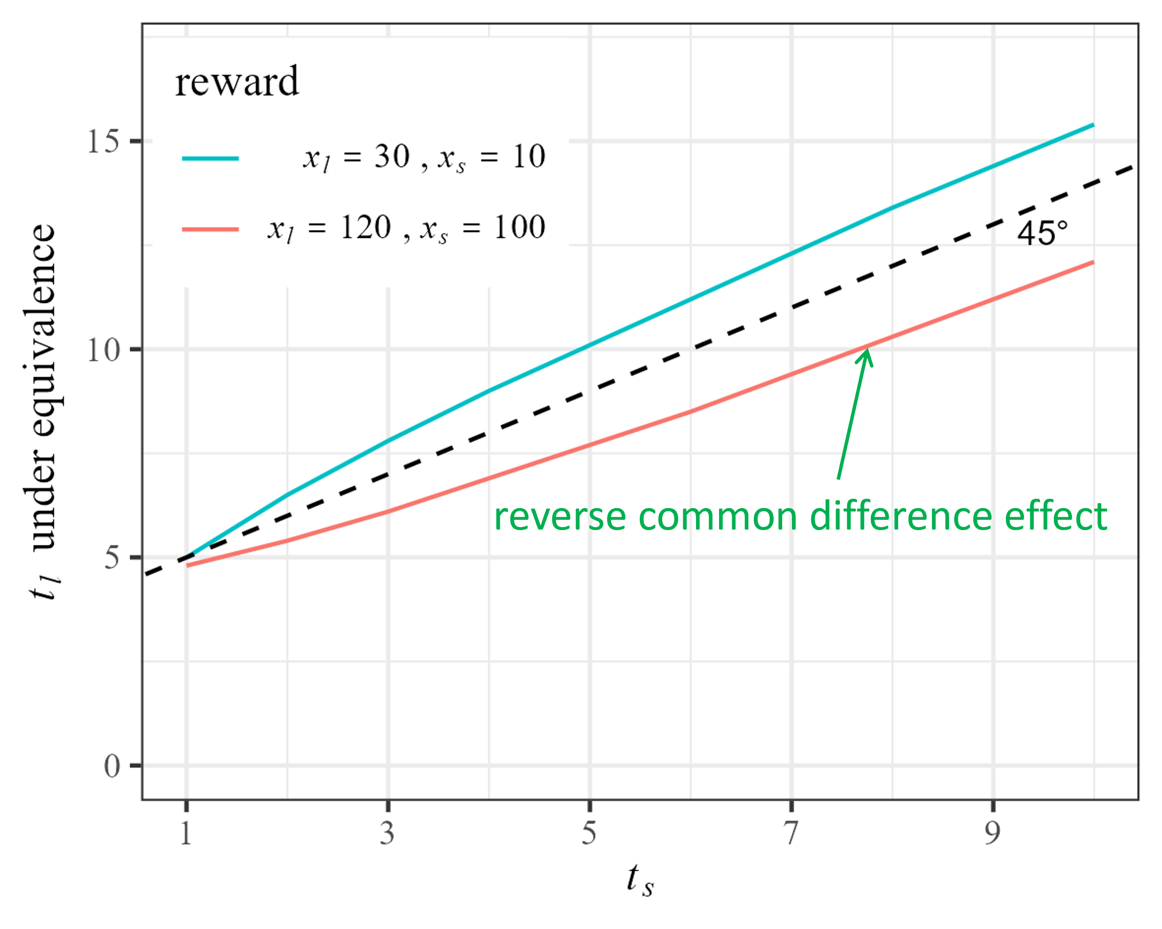
Note: $x_{l}$ and $x_{s}$ are the positive reward levels for LL and SS. The values of LL and SS are calculated based on Equation (4). $d_{t}=0.75^{t}$, $u(x)=x^{0.6}$, $\lambda=2$. For each level of $t_{s}$, we identify the delay $t_{l}$ that makes the value of LL equivalent to SS. The blue line (above) demonstrates the common difference effect, and the red line (below) demonstrates the reverse common difference effect.

Figure 2: The common difference effect and its reverse

Figure 2 demonstrates an example for the reverse common difference effect. In the figure, we set $v_{s}=x_{s}^{0.6}$, $v_{l}=x_{l}^{0.6}$, $\delta=0.75$, $\lambda=2$. For each level of the delay $t_{s}$, we identify the longer delay $t_{l}$ that makes the value of LL equivalent to SS. If the common different effect is valid, increasing $t_{s}$ and $t_{l}$ by the same level would make the DM prefer LL. Under this condition, for one unit increase in $t_{s}$, to make LL and SS valued equally, the identified $t_{l}$ should be increased by a time greater than one unit. On the contrary, if the reverse common difference effect is valid, for one unit increase in $t_{s}$, the identified $t_{l}$ should be increased by a time smaller. In Figure 2, the blue line (above) reflects the common different effect, while the red line (below), which has a lower $v_{l}-v_{s}$ and $v_{l}/v_{s}$, reflects the reverse of it.

4.4 Concavity of Discount Function

Many time discounting models, such as exponential and hyperbolic discounting, assume the discount function is convex in time delay. This type of discount function predicts DM is risk seeking over time lotteries. To illustrate, suppose a reward of level $x$ is delivered at period $t_{l}$ with probability $\pi$ and is delivered at period $t_{s}$ with probability $1-\pi$, where $0<\pi<1$. Meanwhile, another reward of the same level is delivered at period $t_{m}$, where $t_{m}=\pi t_{l}+(1-\pi)t_{s}$. Under such discount functions, the DM should prefer the former reward to the latter reward. For instance, she may prefer receiving an amount of money today or in 20 weeks with equal chance, rather than receiving it in 10 weeks with certainty. However, experimental studies suggest that people are often risk averse over time lotteries, i.e. they prefer the reward to be delivered at a certain time (Onay and Öncüler,, 2007; DeJarnette et al.,, 2020).

One way to accommodate risk aversion over time lotteries is to make the discount function concave in terms of delay. Notably, Onay and Öncüler, (2007) find that people are more likely to be risk averse over time lotteries when $\pi$ is small, and to be risk seeking when $\pi$ is large. Given that $t_{m}$ is increasing in $\pi$, we can claim that the discount function should be concave in delay for the near future but convex for the far future. Takeuchi, (2011) find the supportive evidence for this shape of discount function. In Proposition 3, we apply Equation (4) and show that the AMD model produces this shape of discount function when the DM is impatient and the reward level $x$ is large enough.

Proposition 3: Suppose a single reward $x$ is delivered at period $T$. Let $w_{T}$ denote the AMD factor for this reward. If $\delta=1$, then $w_{T}$ is convex in $T$. If $0<\delta<1$, there exist a reward threshold $\underline{x}>0$ and a time threshold $\underline{T}>0$ such that:

1. when $x\leq\underline{x}$, $w_{T}$ is convex in $T$;

2. when $x>\underline{x}$, $w_{T}$ is convex in $T$ given $T\geq\underline{T}$, and it is concave in $T$ given $0<T<\underline{T}$.

The proof of Proposition 3 is in Appendix C. Figure 3(a) demonstrates the convex discount function (blue line, below) and the inverse-S shaped discount function (red line, above) that could be yielded by Equation (4).

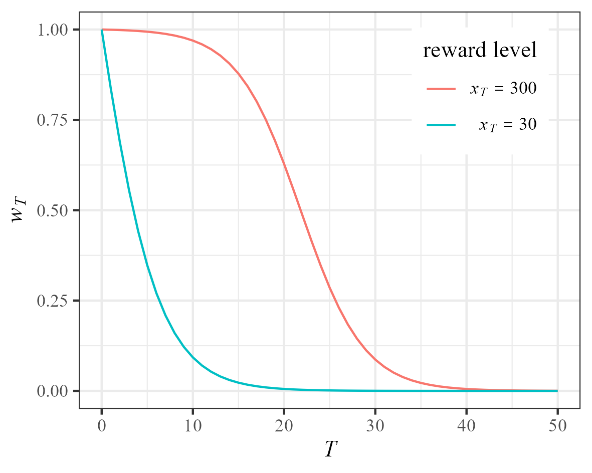
(a) discount function

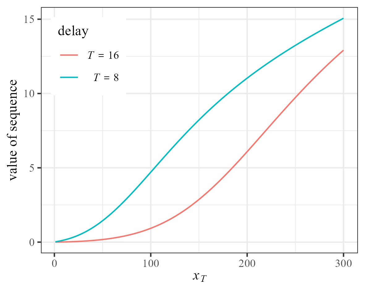
(b) value function

Note: A reward of level $x_{T}$ is delivered at period $T$. The discount function and value function are calculated based on Equation (4). $d_{t}=0.75^{t}$, $u(x)=x^{0.6}$, $\lambda=2$.

Figure 3: Discount function and value function for a delayed reward

4.5 S-Shaped Value Function

A common assumption in decision theories for the instantaneous utility function $u(.)$ is $u^{\prime\prime}<0$. Usually, this implies the value function of a reward is concave. However, empirical evidence suggests that the value functions are often S-shaped. Such S-shaped value functions can be generated by various sources, such as reference dependence (Kahneman and Tversky,, 1979) and efficient coding of numbers (Louie and Glimcher,, 2012). Through the AMD model, we provide a novel account for S-shaped value function based on the insight that larger rewards capture more attention.

Consider a reward of level $x$ delivered at period $T$. Its value function can be represented by $U(x,T)=w_{T}(x)u(x)$. We assume $u^{\prime}>0$, $u^{\prime\prime}<0$, and $w_{T}$ is determined by Equation (4). $w_{T}$ is increasing with $x$ as the DM tends to pay more attention to larger rewards. Both functions $u(x)$ and $w_{T}(x)$ are concave in $x$; so when $x$ is small, they both grow fast. At some conditions, it is possible that the product of the two functions is convex in $x$ when $x$ is small enough. We derive the conditions for the S-shaped value function in Proposition 4.

Proposition 4: Suppose $T\geq 1$, $\frac{d}{dx}\left(\frac{1}{v^{\prime}(x)}\right)$ is continuous in $(0,+\infty)$, then:

1. There exists a threshold $\bar{x}\in\mathbb{R}_{\geq 0}$ such that $U(x,T)$ is strictly concave in $x$ when $x\in[\bar{x},+\infty)$.

2. If $\frac{d}{dx}\left(\frac{1}{v^{\prime}(x)}\right)$ is right-continuous at $x=0$ and $\frac{d}{dx}\left(\frac{1}{v^{\prime}(0)}\right)<1$, there exists $x^{*}\in(0,\bar{x})$ such that, for any $x\in(0,x^{*})$, $U(x,T)$ is strictly convex in $x$.

3. There exists a threshold $\lambda^{*}$ and an interval $(x_{1},x_{2})$ such that, if $\lambda<\lambda^{*}$, for any $x\in(x_{1},x_{2})$, $U(x,T)$ is strictly convex in $x$, where $\lambda^{*}>0$ and $(x_{1},x_{2})\subset(0,\bar{x})$.

The proof of Proposition 4 is in Appendix D. Proposition 4 implies, if the derivative of $\frac{1}{v^{\prime}(x)}$ converges to a small number when $x\rightarrow 0^{+}$, or the unit cost of attention reallocation $\lambda$ is small enough, the value function $U(x,T)$ will be an S-shaped in some interval of $x$. Figure 3(b) demonstrates two examples of this S-shaped value function.

4.6 Intertemporal Correlation Aversion

Consider a DM facing two lotteries, $L1$ and $L2$. For lottery $L1$, she can receive £100 today and £100 in 30 weeks with probability 1/2, and receive £3 today and £3 in 20 weeks with probability 1/2. For lottery $L2$, she can receive £3 today and £100 in 30 weeks with probability 1/2, and receive £100 today and £3 in 20 weeks with probability 1/2. In lottery $L1$, rewards delivered at the two different periods are positively correlated; in lottery $L2$, those rewards are negatively correlated. The expected discounted utility theory predicts the DM is indifferent between the two lotteries. However, recent studies find the evidence of intertemporal correlation aversion (Andersen et al.,, 2018; Rohde and Yu,, 2023). That is, people often prefer lottery $L2$ to $L1$.

For the above example, intertemporal correlation aversion can be explained by the AMD model as follows. The model assumes the allocation of decision weights is within each certain reward sequence, which implies the DM would first aggregate values over time in each state and then calculate the certainty equivalence. For simplicity, suppose there are only two periods. In the state that the DM receives £3 in two periods, suppose she allocates decision weight $w$ to the first period and $1-w$ to the second period. Note when $u(s_{0})=u(s_{1})=...=u(s_{T})$, the AMD factor for every period $t$ remains the same as its default discount factor $d_{t}$. So, in the state that the DM receives £100 in two periods, the decision weights is also the same as $w$ and $1-w$. In the state that the DM can receive £100 in the first period and £3 in the second period, the reward £100 can capture more attention so that its decision weight, say $w^{\prime}$, is greater than $w$. Similarly, in the state that the DM receives £3 earlier and then £100, the decision weight for the later reward £100, say $1-w^{\prime\prime}$, is greater than $1-w$. Therefore, for the lottery in which rewards are positively correlated, its value can be represented by $0.5\cdot u(3)+0.5\cdot u(100)$. Whereas, for the lottery in which rewards are negatively correlated, the value can be represented by $0.5(1-w^{\prime}+w^{\prime\prime})\cdot u(3)+0.5(1-w^{\prime\prime}+w^{\prime})\cdot u(100)$. Given $(1-w^{\prime\prime})+w^{\prime}>1-w+w=1$, the decision weight assigned to $u(100)$, which is $0.5(1-w^{\prime\prime}+w^{\prime})$, should be greater than 0.5. As a result, the DM prefer the latter lottery than the former lottery.

In a more general setting, whether the AMD model can robustly produce intertemporal correlation aversion is influenced by $\lambda$. To see this, we adopt the same definition of intertemporal correlation aversion as Bommier, (2005). Let $(s_{1},s_{2})$ denote the result of a lottery in which the DM can receive reward $s_{1}$ in period $t_{1}$ and then reward $s_{2}$ in period $t_{2}$, where $t_{2}>t_{1}\geq 0$. The results of each lottery is of the same length of sequence. $L1$ generates $(x_{s},y_{s})$ and $(x_{l},y_{l})$ with equal chance, $L_{2}$ generates $(x_{s},y_{l})$ and $(x_{l},y_{s})$ with equal chance, $x_{l}>x_{s}>0$, $y_{l}>y_{s}>0$. By Proposition 5, we show that in this setting, we can always find a $\lambda$ that makes the DM intertemporal correlation averse.

Proposition 5: Suppose $U(L1),U(L2)$ are the values of lotteries $L1$ and $L2$ calculated based on the AMD model. For any $x_{l}>x_{s}>0$, $y_{l}>y_{s}>0$, any default discount factors, and any time length of lottery results, there exists a threshold $\lambda^{**}$ such that for all unit cost of attention reallocation $\lambda\in(\lambda^{**},+\infty)$, we have $U(L1)<U(L2)$, i.e. the DM performs intertemporal correlation aversion.

The proof of Proposition 5 is in Appendix E. The threshold $\lambda^{**}$ is jointly determined by $x_{l}$, $y_{l}$, $y_{s}$, as well as the default discount factors for rewards delivered at $t_{1}$ and $t_{2}$. Notably, when $\lambda\leq\lambda^{**}$, the DM may be intertemporal correlation seeking under some conditions. This suggests a potentially new mechanism for intertemporal correlation aversion, that is, DM performs intertemporal correlation aversion because she attends more to larger rewards while attention reallocation is very costly.

4.7 Concentration Bias

In the existing literature, one approach to modeling attention in intertemporal choice is the focus-weighted utility model (Kőszegi and Szeidl,, 2013). In the focus-weighted utility model, Kőszegi and Szeidl, assume that within a reward sequence, the decision weight for a reward is increasing with the difference of that reward from a reference point. The model predicts that people may perform a concentration bias. Dertwinkel-Kalt et al., (2022) find supportive evidence for this prediction. In this subsection, we show that the AMD model provides an alternative way to generate the concentration bias. Furthermore, we identify the conditions in terms of impatience and attention reallocation cost, which are beyond the predictions of Kőszegi and Szeidl, (2013), for the concentration bias.

To illustrate the concentration bias, consider a DM with a consumption budget £100 to spend over four days (from period 0 to period 3). Suppose the DM has two options: concentrating all consumption at period 0, or splitting the consumption evenly over four periods. The concentration bias implies that she would prefer the first option to the second. We denote the first option as sequence [100,0,0,0] and the second option as sequence [25,25,25,25]. For convenience, we assume the default discount factor for any period $t$ is $d_{t}=\delta^{t}$ and $0<\delta<1$. According to the AMD model, the DM prefers the first option if and only if

$$\frac{e^{u(100)/\lambda}}{e^{u(100)/\lambda}+\delta+\delta^{2}+\delta^{3}}\cdot u(100)>u(25)$$

Obviously, this inequality holds only when $\delta$ or $\lambda$ is small enough, which implies the DM should be very impatient or she can reallocate attention at a very low cost. Notably, under the AMD model, it is also possible that the DM prefers concentrating all consumption at the final period, i.e. the sequence [0,0,0,100], to the second option [25,25,25,25]. In this case, the decision weight multiplied by $u(100)$ in the inequality would become $\frac{\delta^{3}\exp\{u(100)/\lambda\}}{1+\delta+\delta^{2}+\delta^{3}\exp\{u(100)/\lambda\}}$. Then, the inequality holds only when both $\delta$ is large enough and $\lambda$ is small enough. Both cases are in line with the claim in Kőszegi and Szeidl, (2013) and Dertwinkel-Kalt et al., (2022) that the concentration bias can make people behave too impatiently or too patiently.

Next, we derive the conditions for concentration bias in a general optimal-decision setting. From the above example we can draw an intuition that, in a general case, to observe the concentration bias we require the unit cost of attention reallocation $\lambda$ to be small. We show this formally in Proposition 6. Suppose the DM has a consumption budget $m$ ($m>0$) to spend over $T$ periods. Let reward sequence $s_{0\rightarrow T}$ represent her consumption plan at period 0, and let $A\subset\mathbb{R}_{\geq 0}^{T+1}$ denote her alternative space. In period 0, DM wants to find a $s_{0\rightarrow T}$ to solve the optimization problem:

$$\max_{s_{0\rightarrow T}\in A}\;\sum_{t=0}^{T}w_{t}u(s_{t})$$ (5)

where

$$A=\left\{s_{0\rightarrow T}\bigg{|}\;\sum_{t=0}^{T}s_{t}=m,\;\forall t:s_{t}\geq 0\right\}$$

and $w_{t}$ is the AMD factor for consumption in period $t$, subject to default discount factor $d_{t}$. For $s\in[0,m]$, we have $0<u^{\prime}(s)<\infty$, $-\infty<u^{\prime\prime}(s)<0$. Henceforth, we denote the optimization problem in Equation (5) by $\mathcal{O}(m,A,\{d_{t}\}_{t=0}^{T})$. By Proposition 6, we know as long as the DM is impatient (for all period $t<T$, we have $d_{t}>d_{t+1}>0$) and $\lambda$ is small enough, her optimal consumption plan is to consume all of $m$ immediately. The proof of Proposition 6 is in Appendix F.

In Section 2, we state that the unit cost of attention reallocation $\lambda$ has a potential link to cognitive uncertainty. If the DM is highly certain that the default discount factors $\{d_{t}\}_{t=0}^{T}$ truly capture her preference in the local context, she may inhibit the learning about value signals and thus $\lambda$ should be high. This link is also helpful for understanding the relationship between $\lambda$ and concentration bias: when allocating a budget over time, if the DM is totally uncertain about what to do (so $\lambda$ is very small), she may simply concentrate her budget into one period and consume it all.

Proposition 6: Suppose the DM faces the planning problem $\mathcal{O}(m,A,\{d_{t}\}_{t=0}^{T})$, and for all period $t<T$, we have $d_{t}>d_{t+1}>0$. There exists a threshold $\underline{\lambda}>0$ such that for any $\lambda\leq\underline{\lambda}$, her optimal consumption plan is to concentrate all consumption at period 0.

4.8 Inconsistent Planning and Learning

An extensive amount of research evidence suggests that people often exhibit time-inconsistent behaviors in their daily lives (Ericson and Laibson,, 2019). For example, they often consume more than they originally planned, and procrastinate on effortful tasks. In a general sense, such behaviors can be termed present-biased behaviors. Several theories have been proposed for explaining the present-biased behaviors, such as dual-system preferences (Laibson,, 1997), naivete (O’donoghue and Rabin,, 1999), reference dependence (Kőszegi and Rabin,, 2009), and optimistic beliefs (Brunnermeier et al.,, 2017). Based on the AMD model, we can provide an alternative explanation for these behaviors: in dynamic decision-making, people update their default discount factors over time. In more intuitive terms, during each decision step, people will reference their past experiences when allocating attention. If, in the last step, they allocate too much attention to a particular period, they may then take this as a given or default status in the following step and continue to add attention to it. Compared with the existing theoretical explanations, our explanation is built on learning and memory. To perform present-biased behaviors, the DM should recall her mental status at the end of the last step and learn how to allocate attention accordingly. A memoryless DM may perform the reverse behavior. We analyze this with the consumption planning problem in the last subsection.

Again, we suppose the DM has a budget $m$ for consumption. She needs to allocate it over $T$ periods ($T\geq 2$) and the end of sequence is a fixed date. In period 0, her default discount factors $\{d_{t}\}_{t=0}^{T}$ satisfy $d_{t}>d_{t+1}>0$, where $t<T$. When making consumption plan, she would initially weight consumption of period 1 higher than consumption of any other future period. So, she may naturally plan to consume more in period 1 than in period $t=2,…,T$. This in turn, makes her relatively attend more to period 1. Her optimal consumption plan of period 0 should result in $w_{1}/w_{t}>d_{1}/d_{t}$ for each $t=2,…,T$. When arriving in period 1, we assume the DM will use the AMD factors determined in the last step as the new default discount factors. This will lead her to weight consumption of period 1 even higher, and therefore create a motive for over-consumption. In the end, her actual consumption in period 1 will be higher than what has been planned in the last step. Such a trend could continue until she reaches the final period or runs out of money.

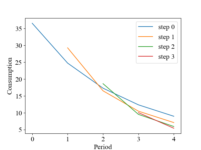
(a) with learning

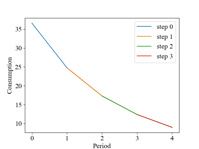
(b) without learning

Note: In step 0, the DM allocates consumption budget $m=100$ over periods 0-4. In step 1, she allocates the remaining consumption over periods 1-4, and so on. “with learning” means the DM updates default discount factors per step; “without learning” means the default discount factors are constant over time. $d_{t}^{0}=0.9^{t}$, $u(x)=x^{0.6}$, $\lambda=70$. Each optimization problem is solved by projection gradient descent method.

Figure 4: Optimal Consumption Plan Over Time

Figure 4 illustrates the relationship between time inconsistency and learning. In the figure, we set $u(x)=x^{0.6}$, $T=4$, $\lambda=70$. At the first step of planning, the DM has a budget of $m=100$ for consumption and her default discount factors are exponential: $d_{t}^{0}=0.9^{t}$. Under the condition “with learning”, which means the DM treats the AMD factors from the optimal consumption plan as default discount factors for the next step, we observe a tendency for over-consumption. Under the condition “without learning”, which means the default discount factors are constant over time, the DM’s behavior is closer to being time-consistent, and in each step, the actual consumption is slightly lower than the consumption planned one step earlier.

We state these results formally in Proposition 7. We focus on the transition from period 0 to period 1, but the conclusions can be expanded to other periods. When the DM plans her consumption in period $j$ ($j=0,1$), the default discount factor for period $t$ is termed $d_{t}^{j}$ and the corresponding AMD factor is termed $w^{j}_{t}$, where $t\geq j$. In the period 0’s optimal consumption plan, the DM plans to consume $s_{t}^{*}$ in period $t$, and in the period 1’s optimal plan, she plans to consume $s_{t}^{**}$. The alternative space is $A$ in period 0 and becomes $A^{\prime}$ in period 1. Notably, to make the time-inconsistency results hold, the DM should not concentrate all consumption into period 0. From Proposition 6, we know that it requires $\lambda$ to be large enough. The proof of Proposition 7 is in Appendix G.

Proposition 7: Suppose the DM faces the planning problem $\mathcal{O}(m,A,\{d^{0}_{t}\}_{t=0}^{T})$ in period 0 and $\mathcal{O}(m-s_{0}^{*},A^{\prime},\{d_{t}^{1}\}_{t=1}^{T})$ in period 1. There exists a threshold $\bar{\lambda}>\underline{\lambda}$ such that when $\lambda\in[\bar{\lambda},+\infty)$, the following is true:

1. In period 0, for any sequence $s_{0\rightarrow T}^{*}\in\{s_{0\rightarrow T}|s_{0\rightarrow T}\in A,\forall t<T:s_{t}>s_{t+1}>0\}$, there exist a specification of default discount factors $\{d_{t}^{0}\}_{t=0}^{T}$, where for all $t<T$ we have $d_{t}^{0}>d_{t+1}^{0}>0$, such that $s_{0\rightarrow T}^{*}$ is the optimal consumption plan.

2. Given $s_{0\rightarrow T}^{*}$ as the period 0’s optimal consumption plan, if in period 1, for all $t\geq 1$ we have $d_{t}^{1}=d_{t}^{0}$, then there must be $s_{1}^{**}<s_{1}^{*}$; if instead we have $d_{t}^{1}=w_{t}^{0}$, then $s_{1}^{**}>s_{1}^{*}$.

In the part (a) of Proposition 7, we reach an interior solution for the consumption planning problem in period 0. The part (b) suggests that, in this case, if we do not take into account the updating of default discount factors, the DM would perform under-consumption behavior over time. In reverse, if the default discount factors are updated based on the AMD factors formed in the most recent consumption plan, the DM will perform over-consumption behavior. The former reflects the behavior of a DM “without learning”, while the latter reflects how the DM would behave “with learning”.

5 Discussion

5.1 Selection of Sequence Length

In our model, the attention a DM can allocate to each time period is affected by sequence length. When a sequence contains more periods, the average attention she can allocate to each period naturally decreases. In Section 4.1, we discuss how this can generate the hidden zero effect. Nevertheless, in reality, we usually cannot observe the actual sequence length perceived by the people. Researchers using our model may also want to make their own assumptions about sequence length. In this subsection, we discuss three issues related to such assumptions and provide recommendations.

The first issue is about the unit of time. A given duration can be represented as sequences of different lengths depending on the time unit used, such as months or days. For example, “receive £10 in 1 month” and “receive £10 in 30 days” essentially mean the same thing, but the latter seems to involve more units of time. When represented in sequence, the former can be represented by [0,10], and the latter can be [0,0,…,0,10], with 30 zeros before the 10. In “standard” discounting models, the number of zeros before the 10 has no effect on the valuation of the sequence. Whereas, the AMD model predicts that, when the reward sequence is described with more time units, the DM may perceive the waiting period for the £10 payment as longer, thereby discounting its value to a greater extent.

As an illustration, suppose in the exponential discounting model, the monthly discount factor is $\delta$. For sequence [0,10], where each period represents a month, the sequence value can therefore be written as $\delta\times u(10)$. For sequence [0,0,…,0,10], where each periods represents a day and there are 30 zeros, we can directly convert the monthly discount factors to daily discount factors in the exponential discounting model. Thus, the discount factor for period $t$ becomes $\delta^{\frac{1}{30}\cdot t}$, and the sequence value remains unchanged. In contrast, this result does not apply to the AMD model. Again, suppose the default discount factors are exponential. According to Equation (4), the AMD factor for the £10 payment is $1/(1+G(T)e^{-v(10)})$. When periods are months, $G(T)=\delta^{-1}$, whereas when periods are days, $G(T)=\delta^{-1}+\delta^{-\frac{29}{30}}+...+\delta^{-\frac{1}{30}}$. Keeping the parameter $\delta$ unchanged, in the latter case, the value of the £10 payment should be more discounted. This suggests that, if we elicit the DM’s time preference from experiments and use the AMD model to fit the data, then the estimate for $\delta$ should be greater when using the sequence with 30 zeros compared to using the sequence with only one zero.

The AMD model’s prediction that sequences with more time units are more discounted is consistent with the numerosity effect (Pelham et al.,, 1994; Zhang and Schwarz,, 2012; Monga and Bagchi,, 2012). This effect refers to the tendency to overestimate quantity as the number of units increases. To our knowledge, currently there is no clear evidence on how the numerosity effect can affect intertemporal choices. This can be a direction for future research. In practice, we recommend that researchers choose the sequence length that matches the time unit presented to participants. For the given example, if a reward sequence is expressed as “receive £10 in 1 month”, researchers would better represent it as [0,10] rather than a sequence with 30 zeros.

The second issue is about the end of sequence. In this paper, an implicit assumption is that each sequence terminates at the point when the final positive reward is delivered. For example, for a sequence described by “receive £10 in 1 month”, we represent it as [0,10] rather than [0,10,0,0]. As we discussed, many empirical findings can be derived under this assumption. However, under this assumption, the model cannot distinguish between the values of two constant sequences of different lengths. To illustrate, consider a choice between two options: (A) “receive £10 now”; and (B) “receive £10 now, and £10 in 1 month, and £10 in 2 months”. According to this assumption, we represent option (A) by a single-period sequence [10] and option (B) by [10,10,10]. In reality, people would certainly prefer option (B) to (A). But, as the AMD model assumes a constant sum of decision weights, both options will be equally valued at $u(10)$.

We propose a simple remedy for this issue: researchers can assume that the DM always takes into account one additional period, or a constant number of additional periods, when processing each sequence. For example, she represents option (A) as [10,0] and option (B) as [10,10,10,0]. Then, the value of option (B) would be certainly greater than option (A). In Appendix H, we show that adding a period to the end of each sequence does not affect the implications that we have discussed.

The third issue is about the violation of dominance. As stated in Section 3.2, in the AMD model, adding a tiny reward to the end of a sequence decreases the sequence value, and this is consistent with the evidence on the violation of dominance (Scholten and Read,, 2014; Jiang et al.,, 2017). However, this effect does not always occur. For example, when choose between “receive £100 now” with “receive £100 now and £10 in 1 month”, people would certainly prefer the latter. This issue can also be solved by the remedy we propose for the second issue. Figure 5 illustrates how the values of these two sequences, in the AMD model, change as more zeros are added towards the end of each sequence. Under the parameters in the figure, when the number of such additional zeros exceeds two, the value of the latter sequence surpasses that of the former. As the number of additional periods increases, the decision maker becomes less likely to exhibit a violation of dominance.

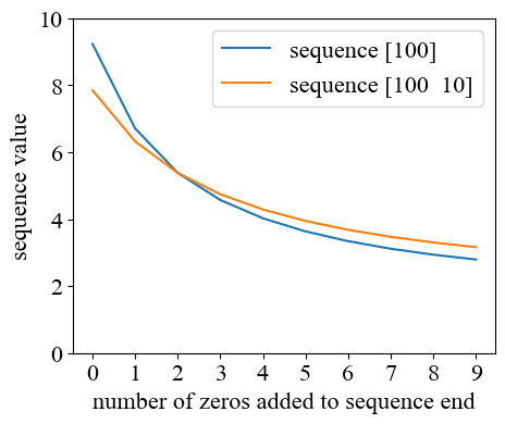
Note: The x-axis denotes the number of additional periods added to a sequence. For example, adding two periods to the sequence [100, 10] would transform it into [100, 10, 0, 0]. $d_{t}^{0}=0.9^{t}$, $u(x)=x^{0.6}$, $\lambda=70$.

Figure 5: The impact of sequence length on sequence value

The rationale for adding a zero (or zeros) to the end of a sequence can be explained as follows. When individuals read the phrase “receive £100 now and £10 in 1 month”, they not only process the information about the two payments, but also infer that the sequence offers no reward beyond the one-month period, even though this is not explicitly described. This implies that, in evaluating the sequence, individuals not only focus on the two described payments but also attend to information regarding the distant future to determine when the sequence ends.

5.2 Relation to Other Intertemporal Choice Models

In the existing literature, the theory most similar to AMD is the salience theory, originally proposed by Bordalo et al., (2012). A recent review (Bordalo et al.,, 2022) summarizes the latest developments in the salience theory. According to that theory, the “salience” of an element in a sequence is increasing with its deviation from a reference point. When the reference point is zero, the salience theory would also predict that people pay more attention to large rewards and less attention to small rewards. Moreover, in Section 4.8, we consider the role of memory and learning in generating time-inconsistent behavior under the AMD model. This is related to Bordalo et al., (2020), which incorporates a memory-based reference point in the salience theory.

Nevertheless, unlike the AMD model, the salience theory does not impose any restrictions on the sum of decision weights; it merely re-normalizes the decision weights. When applied to intertemporal choice, the salience theory represents the value of a sequence by $U=\sum_{t=0}^{T}\pi_{t}w_{t}u(s_{t})$, where $\pi_{t}$ is some “standard” discount factor (e.g. exponential discounting $\pi_{t}=\delta^{t}$), and the re-normalization weight $w_{t}$ is constrained $\sum_{t=0}^{T}w_{t}=1$. As a result, given a sequence [100, 3], transforming it into [100, 3, 3, 3] would have different implications under the salience theory and AMD. In the salience theory, this may make the reward 100 more “salient”, as the total decision weights increase from $\pi_{0}+\pi_{1}$ to $\pi_{0}+\pi_{1}+\pi_{2}+\pi_{3}$, and the reward 100 captures the majority of attention. Whereas, in the AMD model, this operation would reduce the attention allocated to each element.

Some other models also attempt to incorporate attentional mechanisms in intertemporal choice. For example, the focus-weighted utility theory (Kőszegi and Szeidl,, 2013) assumes that people discount large rewards less because they focus on it more, which is the same as AMD. However, in focus-weighted utility theory, this attention shift has no effect on the discount factors of other rewards within the same sequence. Steiner et al., (2017) examine the role of rational inattention in dynamic risky decision-making, and use it to account for inertia and status quo bias. Their theory is grounded in the instrumental utility of information while the AMD model is grounded in its hedonic and cognitive utilities (see Section 3). In psychology, some theories also use random sampling processes to characterize the role of attention in decision-making (Krajbich et al.,, 2010; Johnson and Busemeyer,, 2016), as we did in Section 3.1. Such theories can be applied to fit choice data and explain the underlying information acquisition mechanisms; but, they do not provide specific predictions regarding how people would choose between reward sequences.

5.3 Possible Improvements

There are several ways to improve our model. First, the DM may not just allocate attention within a sequence, but also across sequences. As a result, within the same choice set, the sum of decision weights for one sequence may be smaller than that for another. Researchers interested in this direction can refer to Manzini and Mariotti, (2014) and Gossner et al., (2021). Second, when the DM focuses more on a reward, she may not only assign it greater weight, but also accelerate the rate at which she learns about its value. In our model, the learning rate is controlled by a unified parameter $\lambda$. But in reality, this parameter might vary across different rewards as they capture different levels of attention. Leong et al., (2017) provide an example of analyzing both consequences of attention simultaneously. Third, in the existing literature, the softmax function is usually used to model stochastic choices. Our model examines how this function can be used to study mental representations of reward options. Future research could explore how to integrate these fields to offer a unified behavioral economic framework for analyzing dynamic risky decision-making problems.

Appendix

A. Proof of Proposition 1

We present the proof of sufficiency here. That is, if $\succsim$ has an optimal discounting representation and satisfies Axiom 1-4, then it has an AMD representation.

Lemma 1: If Axiom 1 and 3 hold, for any $s_{0\rightarrow T}$, there exist $w_{0},w_{1},…,w_{T}>0$ such that $s_{0\rightarrow T}\sim w_{0}\cdot s_{0}+...+w_{T}\cdot s_{T}$, where $\sum_{t=0}^{T}w_{t}=1$.

Proof: If $T=1$, Lemma 1 is a direct application of Axiom 3. If $T\geq 2$, for any $2\leq t\leq T$, there should exist $\alpha_{t}\in(0,1)$ such that $s_{0\rightarrow t}\sim\alpha_{t}\cdot s_{0\rightarrow t-1}+(1-\alpha_{t})\cdot s_{t}$. By state-independence and reduction of compound alternatives, we can recursively apply such equivalence relations as follows:

$$s_{0\rightarrow T} \sim\alpha_{T-1}\cdot s_{0\rightarrow T-1}+(1-\alpha_{T-1})\cdot s_{T}$$

$$\sim\alpha_{T-1}\alpha_{T-2}\cdot s_{0\rightarrow T-2}+\alpha_{T-1}(1-\alpha_{T-2})\cdot s_{T-1}+(1-\alpha_{T-1})\cdot s_{T}$$

$$\sim.$$

$$\sim w_{0}\cdot s_{0}+w_{1}\cdot s_{1}+.+w_{T}\cdot s_{T}$$

where $w_{0}=\prod_{t=0}^{T-1}\alpha_{t}$, $w_{T}=1-\alpha_{T-1}$, and for $0<t<T$, $w_{t}=(1-\alpha_{t-1})\prod_{\tau=t}^{T-1}\alpha_{\tau}$. It is easy to show the sum of $w_{0},…,w_{T}$ is equal to 1. QED.

Therefore, if Axiom 1 and 3 hold, for any reward sequence $s_{0\rightarrow T}$, we can always find a convex combination of all its elements, such that the DM is indifferent between the reward sequence and this convex combination. If $s_{0\rightarrow T}$ is a constant sequence, i.e. all its elements are constant, then we can directly assume $\mathcal{W}$ is AMD-style. So henceforth, we discuss whether AMD can apply to non-constant sequences.

By Lemma 2, we show adding a new reward to the end of $s_{0\rightarrow T}$ has no impact on the relative decision weights of rewards in the original reward sequence.

Lemma 2: For any $s_{0\rightarrow T+1}$, if $s_{0\rightarrow T}\sim\sum_{t=0}^{T}w_{t}\cdot s_{t}$ and $s_{0\rightarrow T+1}\sim\sum_{t=0}^{T+1}w^{\prime}_{t}\cdot s_{t}$, where $w_{t},w^{\prime}_{t}>0$ and $\sum_{t=0}^{T}w_{t}=1$, $\sum_{t=0}^{T+1}w^{\prime}_{t}=1$, then when Axiom 1-4 hold, we can obtain $\frac{w^{\prime}_{0}}{w_{0}}=\frac{w^{\prime}_{1}}{w_{1}}=…=\frac{w^{\prime}_{T}}{w_{T}}$.

Proof: According to Axiom 3, for any $s_{0\rightarrow T+1}$, there exist $\alpha,\zeta\in(0,1)$ such that

$$s_{0\rightarrow T}\sim\alpha\cdot s_{0\rightarrow T-1}+(1-\alpha)\cdot s_{T}$$ (A.1)

$$s_{0\rightarrow T+1}\sim\zeta\cdot s_{0\rightarrow T}+(1-\zeta)\cdot s_{T+1}$$

On the other hand, we drawn on Lemma 1 and set

$$s_{0\rightarrow T+1}\sim\beta_{0}\cdot s_{0\rightarrow T-1}+\beta_{1}\cdot s_{T}+(1-\beta_{0}-\beta_{1})\cdot s_{T+1}$$ (A.2)

where $\beta_{0},\beta_{1}>0$. According to Axiom 4, $1-\zeta=1-\beta_{0}-\beta_{1}$. So, $\beta_{1}=\zeta-\beta_{0}$. This also implies $\zeta>\beta_{0}$.

According to Axiom 2, we suppose there exists a reward sequence $s$ such that $s\sim\frac{\beta_{0}}{\zeta}\cdot s_{0\rightarrow T-1}+(1-\frac{\beta_{0}}{\zeta})\cdot s_{T}$. By Equation (A.1) and reduction of compound alternatives, we have $s_{0\rightarrow T+1}\sim\zeta\cdot s+(1-\zeta)\cdot s_{T+1}$. Combining Equation (A.2) with the second line of Equation (A.1) and applying transitivity and state-independence, we obtain $s_{0\rightarrow T}\sim\frac{\beta_{0}}{\zeta}\cdot s_{0\rightarrow T-1}+(1-\frac{\beta_{0}}{\zeta})\cdot s_{1}$.

We aim to prove that for any $s_{0\rightarrow T+1}$, we can obtain $\alpha=\frac{\beta_{0}}{\zeta}$. We show this by contradiction.

Given the symmetry of $\alpha$ and $\frac{\beta_{0}}{\zeta}$, we can assume that $\alpha>\frac{\beta_{0}}{\zeta}$. Consider the case that $s_{0\rightarrow T-1}\succ s_{T}$. By state-independence, for any $c\in\mathbb{R}_{\geq 0}$, we have $(\alpha-\frac{\beta_{0}}{\zeta})\cdot s_{0\rightarrow T-1}+(1-\alpha+\frac{\beta_{0}}{\zeta})\cdot c\succ(\alpha-\frac{\beta_{0}}{\zeta})\cdot s_{T}+(1-\alpha+\frac{\beta_{0}}{\zeta})\cdot c$. By Axiom 2, there exists $z\in\mathbb{R}_{\geq 0}$ such that $(1-\alpha)\cdot s_{T}+\frac{\beta_{0}}{\zeta}\cdot s_{0\rightarrow T-1}\sim z$. Given $c$ is arbitrary, we can set $(1-\alpha+\frac{\beta_{0}}{\zeta})\cdot c\sim z$. By reduction of compound alternatives, we can derive that

$$(\alpha-\frac{\beta_{0}}{\zeta})\cdot s_{0\rightarrow T-1}+(1-\alpha)\cdot s_{T}+\frac{\beta_{0}}{\zeta}\cdot s_{0\rightarrow T-1}\succ(\alpha-\frac{\beta_{0}}{\zeta})\cdot s_{T}+(1-\alpha)\cdot s_{T}+\frac{\beta_{0}}{\zeta}\cdot s_{0\rightarrow T-1}$$

where the LHS can be rearranged to $\alpha\cdot s_{0\rightarrow T-1}+(1-\alpha)\cdot s_{T}$, and the RHS can be rearranged to $\frac{\beta_{0}}{\zeta}\cdot s_{0\rightarrow T-1}+(1-\frac{\beta_{0}}{\zeta})\cdot s_{1}$. They both should be indifferent from $s_{0\rightarrow T}$. This results in a contradiction.

Similarly, in the case that $s_{T}\succ s_{0\rightarrow T-1}$, we can also derive such a contradiction. Meanwhile, when $s_{0\rightarrow T}\sim s_{T}$, $\alpha$ and $\frac{\beta_{0}}{\zeta}$ can be any number within $(0,1)$. In that case, we can directly set $\alpha=\frac{\beta_{0}}{\zeta}$.

Thus, we have $\alpha=\frac{\beta_{0}}{\zeta}$ for any $s_{0\rightarrow T+1}$, which indicates $\frac{\beta_{0}}{\alpha}=\frac{\beta_{1}}{1-\alpha}=\zeta$. We can recursively apply this equality to any sub-sequence $s_{0\rightarrow t}$ ($t\leq T$) of $s_{0\rightarrow T+1}$, so that the lemma will be proved. QED.

Now we move on to prove Proposition 1. The proof contains six steps.

First, we add the constraints $\sum_{t=0}^{T}w_{t}=1$ and $w_{t}>0$ to the optimal discounting problem for $s_{0\rightarrow T}$ so that the problem can accommodate Lemma 1. According to the first-order condition (FOC) of its solution, for all $t=0,1,….,T$, we have

$$f_{t}^{\prime}(w_{t})=u(s_{t})+\theta$$ (A.3)

where $\theta$ is the Lagrange multiplier. Given that $f^{\prime}_{t}(w_{t})$ is strictly increasing, $w_{t}$ is increasing with $u(s_{t})+\theta$. We define the solution as $w_{t}=\phi_{t}(u(s_{t})+\theta)$.

Second, we add a new reward $s_{T+1}$ to the end of $s_{0\rightarrow T}$ and apply Lemma 2 as a constraint on optimal discounting problem. Look at the optimal discounting problem for $s_{0\rightarrow T+1}$. For all $t\leq T$, its FOC should take the same form as Equation (A.3). Hence, if the introduction of $s_{T+1}$ changes some $w_{t}$ to $w^{\prime}_{t}$ ($w^{\prime}_{t}\neq w_{t}$, where $w_{t}$ is the solution to optimal discounting problem for $s_{0\rightarrow T}$), the only way is through changing the multiplier $\theta$. Suppose introducing $s_{T+1}$ changes $\theta$ to $\theta-\Delta\theta$, we have $w^{\prime}_{t}=\phi_{t}(u(s_{t})+\theta-\Delta\theta)$.

By Lemma 2, we know $\frac{w_{0}}{w^{\prime}_{0}}=\frac{w_{1}}{w^{\prime}_{1}}=…=\frac{w_{T}}{w^{\prime}_{T}}$. In other words, for $t=0,1,…,T$, we have $w_{t}\propto\phi_{t}(u(s_{t})+\theta-\Delta\theta)$. We can rewrite $w_{t}$ as

$$w_{t}=\frac{\phi_{t}(u(s_{t})+\theta-\Delta\theta)}{\sum_{\tau=0}^{T}\phi_{\tau}(u(s_{\tau})+\theta-\Delta\theta)}$$ (A.4)

Third, we show that in $s_{0\rightarrow T}$, if we change each $s_{t}$ to $z_{t}$ such that $u(z_{t})=u(s_{t})+\Delta u$, the decision weights $w_{0},…,w_{T}$ will remain the same. Note $\sum_{t=0}^{T}\phi_{t}(u(s_{t})+\theta)=1$. It is clear that $\sum_{t=0}^{T}\phi_{t}(u(z_{t})+\theta-\Delta u)=1$. Suppose changing every $s_{t}$ to $z_{t}$ moves $\theta$ to $\theta^{\prime}$ and $\theta^{\prime}<\theta-\Delta u$. Then, we must have $\phi_{t}(u(z_{t})+\theta^{\prime})<\phi_{t}(u(z_{t})+\theta-\Delta u)$ since $\phi_{t}(.)$ is strictly increasing. Summing all such decision weights up will result in $\sum_{t=0}^{T}\phi_{t}(u(z_{t})+\theta^{\prime})<1$, which contradicts with the constraint that the sum of decision weights is 1. The same contradiction can apply to the case that $\theta^{\prime}>\theta-\Delta u$. Therefore, changing every $s_{t}$ to $z_{t}$ must move $\theta$ to $\theta-\Delta u$, and each $w_{t}$ can only be moved to $\phi_{t}(u(z_{t})+\theta-\Delta u)$, which is exactly the same as the original decision weight.

A natural corollary of this step is that, subtracting or adding a common number to all instantaneous utilities within a reward sequence has no effect on decision weights. What actually matters for determining the decision weights is the difference between these instantaneous utilities. This indicates, for convenience, we can subtract or add an arbitrary number to the utility function.

In other words, for a given $s_{0\rightarrow T}$ and $s_{T+1}$, we can define a new utility function $v(.)$ such that $v(s_{t})=u(s_{t})+\theta-\Delta\theta$. So, Equation (A.4) can be rewritten as

$$w_{t}=\frac{\phi_{t}(v(s_{t}))}{\sum_{\tau=0}^{T}\phi_{\tau}(v(s_{\tau}))}$$ (A.5)

If $w_{t}$ takes the AMD form under the utility function $v(.)$, i.e. $w_{t}\propto d_{t}e^{v(s_{t})/\lambda}$, then it should also take the AMD form under the original utility function $u(.)$.

Fourth, we show that in Equation (A.4), $\Delta\theta$ has two properties: (i) $\Delta\theta$ is strictly increasing with $u(s_{T+1})$; (ii) suppose $\Delta\theta=\underline{\theta}$ when $u(s_{T+1})=\underline{u}$ and $\Delta\theta=\bar{\theta}$ when $u(s_{T+1})=\bar{u}$, where $\underline{u}<\bar{u}$, then for any $l\in(\underline{\theta},\bar{\theta})$, there exists $u(s_{T+1})\in(\underline{u},\bar{u})$ such that $\Delta\theta=l$.

The property (i) can be shown by contradiction. Let $\{w^{\prime}_{t}\}_{t=0}^{T+1}$ denote a sequence of decision weights for $s_{0\rightarrow T+1}$. Suppose $u(s_{T+1})$ is increased but $\Delta\theta$ is constant. In this case, each of $w^{\prime}_{0},…,w^{\prime}_{T}$ should also be constant. However, $w^{\prime}_{T+1}$ should increase as it is strictly increasing with $u(s_{T+1})+\theta-\Delta\theta$ (as $\theta$ is determined only by the optimal discounting problem for $s_{0\rightarrow T}$, any operations on $s_{T+1}$ should have no effect on $\theta$). This contradicts with the constraint that $\sum_{t=0}^{T+1}w^{\prime}_{t}=1$. The only way to avoid such contradictions is to set $\Delta\theta$ strictly increasing with $s_{T+1}$, so that $w^{\prime}_{0},…,w^{\prime}_{T}$ are decreasing with $u(s_{T+1})$.

For property (ii), note that given $s_{0\rightarrow T+1}$ and $\theta$, $\Delta\theta$ is defined as the solution to $\sum_{t=0}^{T+1}\phi_{t}(u(s_{t})+\theta-\Delta\theta)=1$. For any arbitrary number $l\in(\underline{\theta},\bar{\theta})$, the proof of property (ii) consists of two stages. First, for period $t=0,1,…,T$, we need to show $u(s_{t})+\theta-l$ is in the domain of $\phi_{t}(.)$. Second, for period $T+1$, we need to show given any $\omega\in(0,1)$, there exists $u(s_{T+1})\in\mathbb{R}$ such that $\phi_{T+1}(u(s_{T+1})+\theta-l)=\omega$.

For the first stage, note $\phi_{t}(.)$ is the inverse function of $f^{\prime}_{t}(.)$. Suppose when $\Delta\theta=\bar{\theta}$, we have $f^{\prime}_{t}(w^{a}_{t})=u(s_{t})+\theta-\bar{\theta}$, and when $\Delta\theta=\underline{\theta}$, we have $f^{\prime}_{t}(w^{b}_{t})=u(s_{t})+\theta-\underline{\theta}$. For any $l\in(\underline{\theta},\bar{\theta})$, we have $u(s_{t})+\theta-l\in(f^{\prime}_{t}(w^{a}_{t}),f^{\prime}_{t}(w^{b}_{t}))$. Given that $f^{\prime}_{t}(.)$ is continuous and strictly increasing, there must be $w_{t}\in(w^{a}_{t},w^{b}_{t})$ such that $f^{\prime}_{t}(w_{t})=u(s_{t})+\theta-l$. So, $u(s_{t})+\theta-l$ is in the domain of $\theta_{t}(.)$. For the second stage, given an arbitrary $\omega\in(0,1)$, we can directly set $u(s_{T+1})=f^{\prime}(\omega)-\theta+l$, so that the target condition is satisfied.

A corollary of this step is that we can manipulate $\Delta\theta$ in Equation (A.4) at any level between $[\underline{\theta},\bar{\theta}]$ by changing a hypothetical $s_{T+1}$.

Fifth, we show $\ln\phi_{t}(.)$ is linear under some condition. To do this, let us add a hypothetical $s_{T+1}$ to the end of $s_{T}$ and let $w^{\prime}_{t}=\phi_{t}(v(s_{t}))$ denote the decision weights for $s_{0\rightarrow T+1}$. We can change the hypothetical $s_{T+1}$ within the set $\{s_{T+1}|v(s_{T+1})\in[\underline{v},\bar{v}]\}$ and see what will happen to the decision weights from period 0 to period $T$. Suppose this changes each $w^{\prime}_{t}$ to $\phi_{t}(v(s_{t})-\eta)$. Set $\eta=\underline{\eta}$ when $u(s_{T+1})=\underline{v}$ and $\eta=\bar{\eta}$ when $u(s_{T+1})=\bar{v}$. By Equation (A.5), we have

$$\frac{\phi_{t}(v(s_{t}))}{\sum_{\tau=0}^{T}\phi_{\tau}(v(s_{\tau}))}=\frac{\phi_{t}(v(s_{t})-\eta)}{\sum_{\tau=0}^{T}\phi_{\tau}(v(s_{\tau})-\eta)}$$ (A.6)

For each $t=0,1,...,T$, we can rewrite $\phi_{t}(v(s_{t}))$ as $e^{\ln\phi_{t}(v(s_{t}))}$. For the LHS of Equation (A.6), multiplying both the numerator and the denominator by a same number will not affect the value. Therefore, Equation (A.6) can be rewritten as

$$\frac{e^{\ln\phi_{t}(v(s_{t}))-\kappa\eta}}{\sum_{\tau=0}^{T}e^{\ln\phi_{\tau}(v(s_{\tau}))-\kappa\eta}}=\frac{e^{\ln\phi_{t}(v(s_{t})-\eta)}}{\sum_{\tau=0}^{T}e^{\ln\phi_{\tau}(v(s_{\tau})-\eta)}}$$

where $\kappa$ can be any constant number. By properly selecting $\kappa$, for all $t=0,1,...,T$, we can obtain

$$\ln\phi_{t}(v(s_{t}))-\kappa\eta=\ln\phi_{t}(v(s_{t})-\eta)$$ (A.7)

as long as $\eta\in[\underline{\eta},\bar{\eta}]$. Since $\ln\phi_{t}(.)$ is strictly increasing, for any $\eta\neq 0$, we have $\kappa>0$.

Finally, we denote the maximum and minimum of $\{v(s_{t})\}_{t=0}^{T}$ by $v_{\max}$ and $v_{\min}$, and show that Equation (A.7) can hold if $\eta=v_{\max}-v_{\min}$. That implies $v_{\max}-v_{\min}\in[\underline{\eta},\bar{\eta}]$, where $\underline{\eta},\bar{\eta}$ are the realizations of $\eta$ at the points of $v(s_{T+1})=\underline{v}$ and $v(s_{T+1})=\bar{v}$. Obviously, $\underline{\eta}$ can take the value $\underline{\eta}=0$. Thus, we focus on whether $\bar{\eta}$ can take a value $\bar{\eta}\geq v_{\max}-v_{\min}$.

The proof is similar with the fourth step and consists of two stages. First, for $t=0,1,…,T$, we show $v(s_{t})-v_{\max}+v_{\min}$ is in the domain of $\phi_{t}(.)$. That is, under some $w_{t}$, we have $f^{\prime}_{t}(w_{t})=v(s_{t})-v_{\max}+v_{\min}$. Note in a non-constant reward sequence, $v_{\max}-v_{\min}\in(0,+\infty)$. On the one hand, Equation (A.5) indicates that the equation $f^{\prime}_{t}(\omega)=v(s_{t})$ has a solution $\omega$. On the other hand, by Definition 2, we know $\lim_{w_{t}\rightarrow 0}f^{\prime}_{t}(w_{t})=-\infty$. Given $f^{\prime}_{t}(w_{t})$ is continuous and strictly increasing, there must be a solution $w_{t}$ lying in $(0,\omega)$ for equation $f^{\prime}_{t}(w_{t})=v(s_{t})-v_{\max}+v_{\min}$. Second, we show that for any $\omega^{\prime}\in(0,1)$, there exists some $v(s_{T+1})$ such that $\phi_{T+1}(v(s_{T+1})-v_{\max}+v_{\min})=\omega^{\prime}$. This can be achieved by setting $v(s_{T+1})=f^{\prime}_{T+1}(\omega^{\prime})+v_{\max}-v_{\min}$.

As a result, for any period $t$ in $s_{0\rightarrow T}$, by Equation (A.7), we have $\ln\phi_{t}(v(s_{t}))=\ln\phi_{t}(v(s_{t})-\eta)+\kappa\eta$ so long as $\eta\in[0,v_{\max}-v_{\min}]$, where $\kappa>0$. We can rewrite each $\ln\phi_{t}(v(s_{t}))$ as $\ln\phi_{t}(v_{\min})+\kappa[v(s_{t})-v_{\min}]$. Therefore, we have

$$w_{t}\propto\phi_{t}(v_{\min})\cdot e^{\kappa[v(s_{t})-v_{\min}]}$$ (A.8)

and $\sum_{t=0}^{T}w_{t}=1$. In Equation (A.8), setting $\phi_{t}(v_{\min})=d_{t}$, $\lambda=1/\kappa$, and apply the corollary of the third step, we can conclude that $w_{t}\propto d_{t}e^{u(s_{t})/\lambda}$, which is of the AMD form.

B. Proof of Proposition 2

Note the instantaneous utilities of LL and SS are $v_{l}$ and $v_{s}$, and the delays for LL and SS are $t_{l}$ and $t_{s}$. According to Equation (4), the common difference effect implies that, if

$$\frac{v_{s}}{1+G(t_{s})e^{-v_{s}}}=\frac{v_{l}}{1+G(t_{l})e^{-v_{l}}}$$ (B.1)

then for any $\Delta t\geq 0$, we have

$$\frac{v_{s}}{1+G(t_{s}+\Delta t)e^{-v_{s}}}<\frac{v_{l}}{1+G(t_{l}+\Delta t)e^{-v_{l}}}$$ (B.2)

If $G(T)=T$, we have $G(t+\Delta t)=G(t)+\Delta t$. In this case, combining Equation (B.1) and (B.2), we can obtain

$$\frac{\Delta te^{-v_{s}}}{v_{s}}>\frac{\Delta te^{-v_{l}}}{v_{l}}$$ (B.3)

Given that function $\psi(v)=e^{-v}/v$ is decreasing with $v$ so long as $v>0$, Equation (B.3) is valid.

If $G(T)=\frac{1}{1-\delta}(\delta^{-T}-1)$, we have

$$1+G(t+\Delta t)e^{-v}=\delta^{-\Delta t}[1+G(t)e^{-v}]+(\delta^{-\Delta t}-1)(\frac{e^{-v}}{1-\delta}-1)$$ (B.4)

Thus, combining Equation (B.1) and (B.2), we can obtain

$$(\delta^{-\Delta t}-1)\frac{\frac{e^{-v_{s}}}{1-\delta}-1}{v_{s}}>(\delta^{-\Delta t}-1)\frac{\frac{e^{-v_{l}}}{1-\delta}-1}{v_{l}}$$ (B.5)

Given that $0<\delta<1$, we have $\delta^{-\Delta t}>1$. So, Equation (B.5) is valid if and only if

$$\frac{1}{v_{s}}-\frac{1}{v_{l}}<\frac{1}{1-\delta}(\frac{e^{-v_{s}}}{v_{s}}-\frac{e^{-v_{l}}}{v_{l}})$$ (B.6)

By Equation (B.1), we know that

$$\frac{1}{v_{s}}-\frac{1}{v_{l}}=\frac{1}{1-\delta}\left[\frac{(\delta^{-t_{l}}-1)e^{-v_{l}}}{v_{l}}-\frac{(\delta^{-t_{s}}-1)e^{-v_{s}}}{v_{s}}\right]$$ (B.7)

Combining Equation (B.6) and (B.7), we have

$$\delta^{-t_{l}}\frac{e^{-v_{l}}}{v_{l}}<\delta^{-t_{s}}\frac{e^{-v_{s}}}{v_{s}}\Longleftrightarrow v_{l}-v_{s}+\ln\left(\frac{v_{l}}{v_{s}}\right)>-(t_{l}-t_{s})\ln\delta$$

C. Proof of Proposition 3

Suppose a positive reward $x$ is delivered at period $T$. By Equation (4), if $w_{T}$ is convex in $T$, we should have $\frac{\partial^{2}w_{T}}{\partial T^{2}}\geq 0$. This implies

$$2G^{\prime}(T)^{2}\geq(G(T)+e^{v(x)})G^{\prime\prime}(T)$$ (C.1)

If $\delta=1$, then $G(T)=T$. We have $G^{\prime}(T)=1$, $G^{\prime\prime}(T)=0$. Thus, Equation (C.1) is always valid.

If $0<\delta<1$, then $G(T)=(1-\delta)^{-1}(\delta^{-T}-1)$. We have $G^{\prime}(T)=(1-\delta)^{-1}(-\ln\delta)\delta^{-T}$, $G^{\prime\prime}(t)=(-\ln\delta)G^{\prime}(T)$. Thus, Equation (C.1) is valid when

$$\delta^{-T}\geq(1-\delta)e^{v(x)}-1$$ (C.2)

Given $T>0$, Equation (C.2) holds true in two cases. The first case is $1\geq(1-\delta)e^{v(x)}-1$, which implies that $v(x)$ is no greater than a certain threshold $v(\underline{x})$, where $v(\underline{x})=\ln(\frac{2}{1-\delta})$. The second case is that $v(x)$ is above $v(\underline{x})$ and $T$ is above a threshold $\underline{t}$. In the second case, we can take the logarithm on both sides of Equation (C.2). It yields $\underline{t}=\frac{\ln[(1-\delta)\exp\{v(x)\}-1]}{\ln(1/\delta)}$.

D. Proof of Proposition 4

For convenience, we use $v$ to represent $v(x)\equiv u(x)/\lambda$, and use $U$ to represent $U(x,T)$. Set $g=G(T)$. The first-order derivative of $U$ with respect to $x$ can be written as

$$\frac{\partial U}{\partial x}=v^{\prime}\frac{e^{v}+U}{e^{v}+g}$$ (D.1)

If $U$ is strictly concave in $x$, we should have $\frac{\partial^{2}U}{\partial x^{2}}<0$. By Equation (D.1), we calculate the second-order derivative of $U$ with respect to $x$, and rearrange this second-order condition to

$$2\zeta(v)+\frac{1}{1+v\zeta(v)}-1<\frac{-v^{\prime\prime}}{(v^{\prime})^{2}}\equiv\frac{d}{dx}\left(\frac{1}{v^{\prime}}\right)$$ (D.2)

where $\zeta(v)=g/(g+e^{v})$. Since $v^{\prime\prime}<0$, the RHS of Equation (D.2) is clearly positive.

To prove the first part of Proposition 4, we can show that when $x$ is large enough, the LHS of Equation (D.2) will be non-positive. To make the LHS non-positive, we require

$$\zeta(v)+\frac{1}{v}\leq\frac{1}{2}$$ (D.3)

hold true. Note that $\zeta(v)$ is decreasing in $v$, and $v$ is increasing in $x$. Hence, $\zeta(v)+\frac{1}{v}$ is decreasing in $x$. Besides, it approaches $+\infty$ when $x\rightarrow 0$ and approaches 0 when $x\rightarrow+\infty$. When $\frac{d}{dx}\left(\frac{1}{v^{\prime}(x)}\right)$ is continuous, there must be a unique realization of $x$ in $(0,+\infty)$, say $\bar{x}$, making the equality in Equation (D.3) valid. Moreover, when $x\geq\bar{x}$, Equation (D.3) is always valid. In such cases, $U(x,T)$ is concave in $x$.

To prove the second part, first note that when $x=0$, the LHS of Equation (D.2) will become $\frac{2g}{g+1}$. If $\frac{d}{dx}\left(\frac{1}{v^{\prime}(0)}\right)$ is smaller than this number, then the LHS of Equation (D.2) should be greater than the RHS at the point of $x=0$. Meanwhile, from the first part of the current proposition, we know the LHS is smaller than the RHS at the point of $x=\bar{x}$. Thus, given $\frac{d}{dx}\left(\frac{1}{v^{\prime}(x)}\right)$ is continuous in $[0,\bar{x}]$, there must also be a point within $[0,\bar{x}]$, such that the LHS equals the RHS. Let $x^{*}$ denote the minimum of $x$ that makes the equality valid. Then, for any $x\in(0,x^{*})$, we must have that the LHS of Equation (D2) is greater than the RHS, which implies $U(x,T)$ is convex in $x$. Given that $T\geq 1$, we have $g\geq 1$ and thus $\frac{2g}{g+1}\geq 1$. Therefore, when $\frac{d}{dx}\left(\frac{1}{v^{\prime}(0)}\right)<1$, $U(x,t)$ can be convex in $x$ for any $x\in(0,x^{*})$, regardless of $g$.

The prove the third part, note $v(x)=u(x)/\lambda$. So,

$$\frac{d}{dx}\left(\frac{1}{v^{\prime}}\right)=\lambda\frac{d}{dx}\left(\frac{1}{u^{\prime}}\right)$$

We arbitrarily draw a point from $(0,\bar{x})$ and derive the range $\lambda$ relative to this point. For simplicity, we choose $x=\ln g$. In this case, the LHS of Equation (D.2) becomes $\frac{2}{2+\ln g}$. Define a function $\xi(x)$, where $\xi$ is the value of the LHS of Equation (D.2) minus its RHS. Note $\xi(x)$ is continuous at $x=\ln g$. Therefore, for any positive real number $b$, there must exist a positive real number $c$ such that, when $x\in(\ln g-c,\ln g+c)$, we have

$$\xi(\ln g)-b<\xi(x)<\xi(\ln g)+b$$ (D.4)

If $\xi(\ln g)-b\geq 0$, then $\xi(x)$ will keep positive for all $x\in(\ln g-c,\ln g+c)$, which implies the LHS of Equation (D.2) is always greater than its RHS.

Now we derive the condition for $\xi(\ln g)-b\geq 0$. Suppose when $x=\ln g$, $\frac{d}{dx}\left(\frac{1}{u^{\prime}}\right)=a$ (note at this point we have $\frac{d}{dx}\left(\frac{1}{u^{\prime}}\right)<+\infty$). Combining with Equation (D.3), we know that $\xi(\ln g)-b=\frac{2}{2+\ln g}-\lambda a-b$. Letting this value be non-negative, we obtain

$$\lambda\leq\frac{2}{a(2+\ln g)}-\frac{b}{a}$$ (D.5)

Given that $T\geq 1$, we have $g\geq 1$ and thus $\frac{2}{2+\ln g}$ should be positive. Meanwhile, given that $u^{\prime}>0$ and $u^{\prime\prime}<0$, $a$ should also be positive. Since $b$ can be any positive number, Equation (D.5) holds if $\lambda<\frac{2}{a(2+\ln g)}$. That is, when $\lambda$ is positive but smaller than a certain threshold, there must be an interval $(\ln g-c,\ln g+c)$ such that the LHS of Equation (D.2) is greater than the RHS. Set $x_{1}=\max\{0,\ln g-c\}$, $x_{2}=\min\{\bar{x},\ln g+c\}$. When $x\in(x_{1},x_{2})$, function $U(x,T)$ must be convex in $x$.

E. Proof of Proposition 5

The proof consists of four steps. First, we write the expressions for $U(L1)$ and $U(L2)$. Suppose the time length of each lottery result is $T$. For a period $\tau$ at which no reward is delivered, the instantaneous utility is zero. Let $\Omega$ denote the set of all such period $\tau$, then $\Omega=\{\tau\,|\,0\leq\tau\leq T,\;\tau\neq t_{1},t_{2}\}$. For any $j,k\in\{s,l\}$, we define $\phi_{j}=d_{t_{1}}e^{v(x_{j})}$ and $\eta_{k}=d_{t_{2}}e^{v(y_{k})}$, where $v(s)=u(s)/\lambda$, and $d_{t}$ represents the default discount factor for reward delivered at period $t$.

For a given lottery result $(s_{1},s_{2})$, we denote the decision weight of each positive reward by $w_{t_{1}}$ and $w_{t_{2}}$. By the definition of AMD, we have

$$w_{t_{1}}=\frac{\phi_{j}}{\phi_{j}+\eta_{k}+D}\quad,\quad w_{t_{2}}=\frac{\eta_{k}}{\phi_{j}+\eta_{k}+D}$$

where $j,k\in\{s,l\}$, $D=\sum_{\tau\in\Omega}d_{\tau}\geq 0$. The value of a lottery $L$ can be written as $U(L)=w_{t_{1}}u(s_{1})+w_{t_{2}}u(s_{2})$. Hence,

$$U(L1)=5\frac{\phi_{s}u(x_{s})+\eta_{s}u(y_{s})}{\phi_{s}+\eta_{s}+D}+5\frac{\phi_{l}u(x_{l})+\eta_{l}u(y_{l})}{\phi_{l}+\eta_{l}+D}$$ (E.1)

$$U(L2)=5\frac{\phi_{s}u(x_{s})+\eta_{l}u(y_{l})}{\phi_{s}+\eta_{l}+D}+5\frac{\phi_{l}u(x_{l})+\eta_{s}u(y_{s})}{\phi_{l}+\eta_{s}+D}$$

We observe that, when $x_{l}=x_{s}$, we have $U(L1)=U(L2)$.

Second, suppose we increase $x_{l}$ from $x_{s}$ by an increment. This increases both $U(L1)$ and $U(L2)$ (either by a positive or a negative number). To make $U(L1)<U(L2)$, this increment should increase $U(L2)$ by a greater number than $U(L1)$. Specifically, we assume $U(L2)$ is increasing faster than $U(L1)$ at any level of $x_{l}$. That is, the partial derivative of $U(L2)$ in terms of $x_{l}$ is always greater than that of $U(L1)$. Given $\phi_{l}$ is increasing in $x_{l}$, to see this, we can take partial derivatives in terms of $\phi_{l}$.

In each line of Equation (E.1), note only the second term contains $x_{l}$. Thus, we focus on the difference between the second terms. The second term of the $U(L1)$ is influenced by $y_{l}$, while that of the $U(L2)$ is influenced by $y_{s}$, where $y_{l}>y_{s}$. Thus, we can construct a function $\xi$ such that

$$\xi(\phi_{l},\eta)=\frac{\phi_{l}\cdot v(x_{l})+\eta\cdot v(y)}{\phi_{l}+\eta+D}$$

where $\eta=d_{t_{2}}e^{v(y)}$. In reverse, we can define $v(x_{l})=\ln(\phi_{l}/d_{t_{1}})$ and $v(y)=\ln(\eta/d_{t_{2}})$. The function $\xi$ is similar to the second term of each line, but note we replace $u(.)$ by $v(.)$. When $y=y_{l}$, $\xi$ is proportional to the second term of $U(L1)$. When $y=y_{s}$, $\xi$ is proportional to the second term of $U(L2)$ (by the same proportion). Thus, to show that the partial derivative of $U(L2)$ in terms of $x_{l}$ is greater than that of $U(L1)$, we just need to show $\partial\xi/\partial\phi_{l}$ is decreasing with $y$ (or $\eta$).

Third, we take the first- and second-order partial derivatives of $\xi(\phi_{l},\eta)$. The partial derivative of $\xi$ in terms of $\phi_{l}$ is

$$\frac{\partial\xi}{\partial\phi_{l}}=\frac{(v(x_{l})+1)\eta-v(y)\eta+\phi_{l}+D(v(x_{l})+1)}{(\phi_{l}+\eta+D)^{2}}$$

We need to show that for $y\in[y_{s},y_{l}]$, we can obtain $\partial^{2}\xi/\partial\phi_{l}\partial\eta<0$. This implies

$$(v(x_{l})+v(y)+2)D-(\phi_{l}-\eta)(v(x_{l})-v(y))+2(\phi_{l}+\eta)>0$$ (E.2)

We want Equation (E.2) to hold for any $D\geq 0$. Given the LHS is increasing with $D$, this can only be achieved when

$$2(\phi_{l}+\eta)>(\phi_{l}-\eta)(v(x_{l})-v(y))$$ (E.3)

Define $\kappa=d_{t_{2}}/d_{t_{1}}$, $\alpha=v(x_{l})-v(y)$. Note $\kappa\in\mathbb{R}_{>0}$, $\alpha\in\mathbb{R}$. Equation (E.3) can be rewritten as

$$(\alpha-2)\kappa^{-1}e^{\alpha}-\alpha-2<0$$ (E.4)

Fourth, based on Equation (E.4), we construct a function $h(\alpha)=(\alpha-2)\kappa^{-1}e^{\alpha}-\alpha-2$. We aim to examine whether there exists some $\alpha\in\mathbb{R}$ that makes $h(a)<0$. Obviously, $\alpha=-2$ and $\alpha=2$ satisfy this condition. Moreover, note $h(\alpha)$ is decreasing in $\alpha$ when $(\alpha-1)e^{\alpha}\leq\kappa$ and is increasing in $\alpha$ otherwise. And when either $\alpha\rightarrow-\infty$ or $\alpha\rightarrow+\infty$, we have $h(\alpha)\rightarrow+\infty$. Thus, there must be a limited interval $(\alpha_{1},\alpha_{2})$ such that $h(a)<0$ so long as $\alpha\in(\alpha_{1},\alpha_{2})$, and obviously $[-2,2]\subset(\alpha_{1},\alpha_{2})$. Since $v(s)=u(s)/\lambda$, this implies $\frac{u(x_{l})-u(y)}{\lambda}\in(\alpha_{1},\alpha_{2})$.

For a given positive number $\kappa$, the points $\alpha_{1},\alpha_{2}$ are determined by the solution to $\frac{\alpha-2}{\alpha+2}e^{\alpha}=\kappa$. In other words, for any $x_{l}$ and $y\in[y_{s},y_{l}]$, we can always achieve $U(L1)<U(L2)$ as long as $u(x_{l})-u(y_{l})\geq\lambda\alpha_{1}$ and $u(x_{l})-u(y_{s})\leq\lambda\alpha_{2}$. So, we can conclude that for any $x_{l}>x_{s}>0$, $y_{l}>y_{s}>0$, any time length of lottery results and default discount factor (which determines $D$ and $\kappa$), there exists some $\lambda$ that makes DM intertemporal correlation averse. Specifically, all $\lambda>\lambda^{**}={\max}\{\frac{u(x_{l})-u(y_{l})}{\alpha_{1}},\frac{u(x_{l})-u(y_{s})}{\alpha_{2}}\}$ satisfy the target condition.

Notably, if $\lambda\leq\lambda^{**}$, we have $h(a)\geq 0$, which by Equation (E.2)(E.3), indicates that under some conditions such as $D=0$, there will be $\partial^{2}\xi/\partial\phi_{l}\partial\eta\geq 0$ for all $y\in[y_{s},y_{l}]$. In that case, at each level of $x_{l}$, the partial derivative of $U(L1)$ in terms of $x_{l}$ is greater than that of $U(L2)$. So, increasing $x_{l}$ by an increment from $x_{s}$ can induce a greater increase in $U(L1)$ than in $U(L2)$. This makes it possible that $U(L1)>U(L2)$. In short, DM may perform intertemporal correlation seeking when $\lambda\leq\lambda^{**}$.

F. Proof of Proposition 6

Before proving the proposition, we first show that in the DM’s optimal consumption plan $s_{0\rightarrow T}$, the largest consumption must be $s_{0}$. To show this, suppose the largest consumption is $s_{\tau}$ ($\tau>0$). By Lemma 3 below, we can obtain that if we exchange the consumption planned in $\tau$ with the consumption planned in period 0, the total value of consumption will be non-decreasing. So, the largest consumption must be placed in period 0.

For convenience, henceforth we use $u_{t}$ to represent $u(s_{t})$.

Lemma 3: Suppose in $s_{0\rightarrow T}$, we have $s_{\tau}=\max\{s_{0},s_{1},...,s_{T}\}$ and $\tau>0$. Set $u_{0}/\lambda=v_{1}$ and $u_{\tau}/\lambda=v_{2}$. If we change $u_{0}/\lambda$ to $v_{2}$ and $u_{\tau}/\lambda$ to $v_{1}$, $U(s_{0\rightarrow T})$ will be non-decreasing.

Proof: Let $V/\lambda$ denote the total value of consumption before we exchange consumption between period 0 and $\tau$, where

$$V=\frac{\sum_{t=0}^{T}(u_{t}/\lambda)\cdot d_{t}e^{u_{t}/\lambda}}{\sum_{t=0}^{T}d_{t}e^{u_{t}/\lambda}}$$

Set $d_{0}=\delta_{1}$, $d_{\tau}=\delta_{2}$. We denote the numerator of $V$ by $v_{1}\delta_{1}e^{v_{1}}+v_{2}\delta_{2}e^{v_{2}}+P$ and denote its denominator by $\delta_{1}e^{v_{1}}+\delta_{2}e^{v_{2}}+Q$.

Note $v_{2}\geq V$. If changing $u_{t}/\lambda$ to $v_{2}$ as well as $u_{t+\tau}/\lambda$ to $v_{1}$ does not decrease $V$, we should have

$$\frac{v_{1}\delta_{1}e^{v_{1}}+v_{2}\delta_{2}e^{v_{2}}+P}{\delta_{1}e^{v_{1}}+\delta_{2}e^{v_{2}}+Q}\leq\frac{v_{2}\delta_{1}e^{v_{2}}+v_{1}\delta_{2}e^{v_{1}}+P}{\delta_{1}e^{v_{2}}+\delta_{2}e^{v_{1}}+Q}$$ (F.1)

where $\delta_{1}>\delta_{2}>0$, $v_{2}\geq v_{1}>0$. By rearranging Equation (F.1), we can obtain

$$-(\delta_{1}+\delta_{2})e^{v_{1}+v_{2}}(v_{2}-v_{1})\leq e^{v_{2}}(Qv_{2}-P)-e^{v_{1}}(Qv_{1}-P)$$ (F.2)

Clearly, Equation (F.2) holds if $e^{v}(Qv-P)$ is increasing with $v$ when $v\in[v_{1},v_{2}]$, and the latter implies $v_{1}\geq\frac{P}{Q}-1$.

Notably, $V$ is a weighted mean of $v_{1}$, $v_{2}$ and $\frac{P}{Q}$, and we have $v_{2}\geq\max\{v_{1},\frac{P}{Q}\}$. If $v_{1}\geq V$, we must have $v_{1}\geq\frac{P}{Q}$. In this case, Equation (F.2) clearly holds. If $v_{1}<V$, note that $\frac{\partial U}{\partial d_{t}}\propto u_{t}-U$. So, we will have $\frac{\partial U}{\partial d_{0}}<0$ and $\frac{\partial U}{\partial d_{\tau}}>0$. Both decreasing $d_{0}$ to $\delta_{2}$ and increasing $d_{\tau}$ to $\delta_{1}$ would increase the total value of consumption. In summary, for either case, after changing $u_{t}/\lambda$ to $v_{2}$ and $u_{t+\tau}/\lambda$ to $v_{1}$, $V$ should be non-decreasing. QED.

Denote the value of $s_{0\rightarrow T}$ by $U=\sum_{t=0}^{T}w_{t}u(s_{t})$. Notably, if the optimal consumption plan is an interior solution, then the solution must satisfy $\frac{\partial U}{\partial s_{t+1}}/\frac{\partial U}{\partial s_{t}}=1$. Suppose $\frac{\partial U}{\partial s_{t}}>\frac{\partial U}{\partial s_{t+1}}>0$, then the DM can transfer an incremental consumption from $s_{t+1}$ to $s_{t}$, as increasing $s_{t}$ by an increment will lead to a greater improvement in $U$ compared to the decrease in $U$ caused by reducing $s_{t+1}$ by the same amount. The DM will keep transfer consumption between periods until $\frac{\partial U}{\partial s_{t}}=\frac{\partial U}{\partial s_{t+1}}$. Nevertheless, if the DM keeps reducing $s_{t+1}$ and still has $\frac{\partial U}{\partial s_{t}}>\frac{\partial U}{\partial s_{t+1}}>0$ even when $s_{t+1}$ is reduced to 0, this optimization problem will reach a corner solution. We aim to show that when $\lambda$ is small enough, for all $t>0$, the DM would tend to reduce $s_{t}$ to zero.

The partial derivatives of $U$ in terms of $s_{t}$ is $\frac{\partial U}{\partial s_{t}}=w_{t}u^{\prime}_{t}(u_{t}+\lambda-U)$. Therefore, we have

$$\frac{\partial U}{\partial s_{t+1}}/\frac{\partial U}{\partial s_{t}}=\frac{d_{t+1}}{d_{t}}\exp\{\frac{u_{t+1}-u_{t}}{\lambda}\}\cdot\frac{u^{\prime}_{t+1}}{u^{\prime}_{t}}\cdot\frac{u_{t+1}+\lambda-U}{u_{t}+\lambda-U}$$ (F.3)

Drawing on Equation (F.3), we construct a function $\rho(s_{t};\mathcal{U})=e^{u_{t}/\lambda}u^{\prime}_{t}(u_{t}+\lambda-\mathcal{U})$. Its partial derivative in terms of $s_{t}$ is

$$\frac{\partial\rho(s_{t};\mathcal{U})}{\partial s_{t}}=e^{u_{t}/\lambda}[(u_{t}+\lambda-\mathcal{U})(\frac{(u^{\prime}_{t})^{2}}{\lambda}+u^{\prime\prime}_{t})+(u^{\prime}_{t})^{2}]$$ (F.4)

To prove Proposition 6, note that if

$$\lambda\leq\min_{0\leq t\leq T}\;\inf_{s_{0\rightarrow T}\in A}\{-(u^{\prime}_{t})^{2}/u^{\prime\prime}_{t}\}$$ (F.5)

we will always have $\frac{(u^{\prime}_{t})^{2}}{\lambda}+u^{\prime\prime}_{t}\geq 0$. Set $\underline{\lambda}$ as the RHS of Equation (F.5). Note by Lemma 3, we know that $s_{0}$ must be the largest consumption in the DM’s consumption plan. It can be proved that if $\lambda\leq\underline{\lambda}$, in an arbitrary sequence $s_{0\rightarrow T}$ that satisfies this condition, it is always beneficial for the DM to transfer consumption from the future periods to the current period, until all consumption is concentrated at the current period. We discuss this in two cases.

First, suppose for all $t>0$, we have $u_{t}+\lambda-U>0$. As $s_{0}$ is the largest consumption, we must have $u_{0}>U$; so, we also have $u_{0}+\lambda-U>0$. In this case, if $\lambda\leq\underline{\lambda}$, according to Equation (F.4), we can obtain $\frac{\partial\rho(s_{t};U)}{\partial s_{t}}>0$. By Equation (F.3), for all $t>0$, we have $\frac{\partial U}{\partial s_{t}}/\frac{\partial U}{\partial s_{0}}=\frac{d_{t}}{d_{0}}\frac{\rho(s_{t};U)}{\rho(s_{0};U)}$. Since $d_{0}>d_{t}$ and $s_{0}>s_{t}$, we can obtain $\frac{\partial U}{\partial s_{0}}>\frac{\partial U}{\partial s_{t}}>0$. Therefore, it is beneficial for the DM to transfer an incremental consumption from $s_{t}$ to $s_{0}$.

Second, suppose for some period $\tau>0$, we have $u_{\tau}+\lambda-U<0$. For this period $\tau$, there must be $\frac{\partial U}{\partial s_{\tau}}<0$. A reduction in $s_{\tau}$ will increase $U$. So, it is also beneficial to reduce it and transfer the consumption to the current period.

In conclusion, in any sequence, as long as $s_{0}$ is the largest consumption, transferring consumption from the future to the present must improve $U$. If in such a sequence, a future period has a positive consumption, the DM will keep transfer it to the current period until she concentrates all consumption into the current period.

G. Proof of Proposition 7

We use the same notation as in the proof of Proposition 6. Before proving Proposition 7, we list a set of conditions that, taken together, are sufficient to derive the resulting behavior in the proposition. We then prove that all these conditions are satisfied as long as $\lambda$ is large enough.

First, suppose the consumption planing problem has an interior solution. Again, let $U$ denote the value of a consumption sequence. Then, for any period $t$ in the optimal plan, we should have $\frac{\partial U}{\partial s_{t+1}}/\frac{\partial U}{\partial s_{t}}=1$ and $\frac{\partial^{2}U}{\partial s_{t}^{2}}<0$. The second-order condition implies

$$(1-2w_{t})\frac{1}{\lambda}+\frac{1}{u_{t}+\lambda-U}<-\frac{u^{\prime\prime}_{t}}{(u^{\prime}_{t})^{2}}$$ (G.1)

Second, to analyze how a change in $s_{t}$ will affect $\frac{\partial U}{\partial s_{t}}$, we construct a function $\tilde{\rho}_{t}(s_{0},s_{1},...,s_{T})\equiv\rho(s_{t};U)$. By calculating the partial derivative of $\tilde{\rho}_{t}$ in terms of $s_{t}$, when $u_{t}+\lambda-U>0$, we can obtain

$$\frac{\partial\tilde{\rho}_{t}}{\partial s_{t}}<0\;\Longleftrightarrow\;(1-w_{t})\frac{1}{\lambda}+\frac{1}{u_{t}+\lambda-U}<-\frac{u^{\prime\prime}_{t}}{(u^{\prime}_{t})^{2}}$$ (G.2)

Third, when $u_{t}+\lambda-U>0$, according to Equation (F.4), we can also obtain that $\rho(s_{t};U)$ decreases in $s_{t}$ if and only if

$$\frac{1}{\lambda}+\frac{1}{u_{t}+\lambda-U}<-\frac{u^{\prime\prime}_{t}}{(u^{\prime}_{t})^{2}}$$ (G.3)

Clearly, if Equation (G.3) holds, both Equation (G.1) and (G.2) will also hold. Note $u(m)>U$; so, if $\lambda-u(m)\geq 0$, we will always have $u_{t}+\lambda-U>0$. Under this interval of $\lambda$, the LHS of Equation (G.3) is continuous and decreasing in $\lambda$, and it converges to 0 with $\lambda\rightarrow 0$. Hence, there must be some $\bar{\lambda}_{1}\geq u(m)$ such that, when $\lambda\geq\bar{\lambda}_{1}$, for any given consumption sequence, Equation (G.3) is valid.

Fourth, we construct a new function $\Gamma(s_{t};\mathcal{U})=e^{u_{t}/\lambda}\cdot\left(\frac{u_{t}+\lambda}{u_{t}+\lambda-\mathcal{U}}\right)$. By calculating the partial derivative of $\Gamma$ in terms of $s_{t}$, when $u_{t}+\lambda-U>0$, we can obtain

$$\frac{\partial\Gamma(s_{t};U)}{\partial s_{t}}>0\Longleftrightarrow(\lambda+u_{t}-U)^{2}+U(u_{t}-U)>0$$ (G.4)

If $\lambda$ is large enough, Equation (G.4) must hold. Again, we can conclude that there is some $\bar{\lambda}_{2}\geq u(m)$, such that when $\lambda\geq\bar{\lambda}_{2}$, for any given sequence, Equation (G.4) is valid.

We define $\bar{\lambda}$ as $\max\{\bar{\lambda}_{1},\bar{\lambda}_{2}\}$. It can be shown that any $\lambda\in[\bar{\lambda},+\infty)$ satisfies the proposition.

For the part (a) of Proposition 7, note by Equation (F.3), we have $\frac{\partial U}{\partial s_{t+1}}/\frac{\partial U}{\partial s_{t}}=\frac{d_{t+1}}{d_{t}}\frac{\rho(s_{t+1};U)}{\rho(s_{t};U)}$. Given an arbitrary sequence in the set $\{s_{0\rightarrow T}|s_{0\rightarrow T}\in A,\forall t<T:s_{t}>s_{t+1}>0\}$ (the sequence is decreasing and available for choice, and all rewards are positive), when $\lambda\geq\bar{\lambda}$, for each period $t<T$ in the sequence, we have $\rho(s_{t+1};U)>\rho(s_{t};U)$, as $\rho(s_{t};U)$ is decreasing in $s_{t}$.

Denote the given sequence by $s_{0\rightarrow T}^{*}$. To make $s_{0\rightarrow T}^{*}$ become the interior solution for the planning problem in period 0, according to the FOC, we need $\frac{d_{t+1}^{0}}{d_{t}^{0}}=\frac{\rho(s_{t};U)}{\rho(s_{t+1};U)}$. Thus, we can define $d_{t}^{0}$ as

$$d_{t}^{0}=\frac{\rho(s_{t};U)^{-1}}{\rho(s_{0};U)^{-1}+...+\rho(s_{T};U)^{-1}}$$

According to this definition, it can be easily validated that $\frac{d_{t+1}^{0}}{d_{t}^{0}}=\frac{\rho(s_{t};U)}{\rho(s_{t+1};U)}$ and $d_{t}^{0}>d_{t+1}^{0}>0$. Under such $\{d_{t}^{0}\}_{t=0}^{T}$, the given sequence $s_{0\rightarrow T}^{*}$ is the optimal consumption plan.

For the part (b), we prove it in two steps. First, we show if $d_{t}^{1}=d_{t}^{0}$, the DM will under-consume in period 1. In this case, for any $t\geq 1$ we set $d_{t}^{0}=d_{t}^{1}=d_{t}$. Given $s_{0\rightarrow T}^{*}$ as the period 0’s optimal consumption plan, when moving to period 1, the DM will need to allocate budget over period $t=1,…,T$, and the largest consumption $s_{0}^{*}$ will be moved out from the sequence. Keeping everything equal, this will reduce the sequence value $U$, thereby (under the condition $\lambda\geq\bar{\lambda}$) increasing $\frac{u_{t+1}+\lambda-U}{u_{t}+\lambda-U}$. Thus, according to Equation (F3), $\frac{\partial U}{\partial s_{t+1}}/\frac{\partial U}{\partial s_{t}}$ will increase to greater than 1. To optimize the consumption plan, the DM needs to adjust $s_{t}$ and $s_{t+1}$ toward re-achieving $\frac{\partial U}{\partial s_{t+1}}/\frac{\partial U}{\partial s_{t}}=\frac{d_{t+1}}{d_{t}}\frac{\tilde{\rho}_{t+1}}{\tilde{\rho}_{t}}=1$. Specifically, she is required to reduce $\frac{\tilde{\rho}_{t+1}}{\tilde{\rho}_{t}}$. According to Equation (G.2), when $\lambda\geq\bar{\lambda}$, $\tilde{\rho}_{t}$ is decreasing in $s_{t}$, which implies that the DM needs to increase $s_{t+1}$ in relative to $s_{t}$. In other words, she needs to transfer consumption from an earlier period to a later period. So, for the optimal consumption plan in period 1, we have $s_{1}^{**}<s_{1}^{*}$.

Finally, we discuss the case that $d_{t}^{1}=w_{t}^{0}$. When moving to period 1, how the DM will adjust consumption is affected by two mechanisms. On the one hand, as $\frac{d_{t+1}^{1}}{d_{t}^{1}}=\frac{d_{t+1}^{0}}{d_{t}^{0}}\exp\{\frac{u_{t+1}-u_{t}}{\lambda}\}$, the DM will initially pay more attention to an earlier period than a later period; on the other hand, as the largest consumption $s_{0}^{*}$ is moved out, keeping everything equal, the sequence value $U$ will decrease. We suppose it will decrease from $U_{0}$ to $U_{1}$. The former mechanism drives the DM to transfer consumption from a later period to an earlier period, while the latter mechanism drives her to do the opposite. We can show that the former mechanism overrides the latter.

To show this, note for the period 0’s optimal consumption plan, we have $\frac{\partial U}{\partial s_{t+1}}/\frac{\partial U}{\partial s_{t}}=\frac{d_{t+1}^{0}}{d_{t}^{0}}\frac{\rho(s_{t+1}^{*};U_{0})}{\rho(s_{t}^{*};U_{0})}=1$. Substituting it into the equation of $\frac{\partial U}{\partial s_{t+1}}/\frac{\partial U}{\partial s_{t}}$ in period 1 (keeping everything equal), we have

$$\frac{\partial U}{\partial s_{t+1}}/\frac{\partial U}{\partial s_{t}}=\exp\{\frac{u(s_{t+1}^{*})-u(s_{t}^{*})}{\lambda}\}\frac{u_{t+1}+\lambda-U_{1}}{u_{t}+\lambda-U_{1}}\frac{u_{t}+\lambda-U_{0}}{u_{t+1}+\lambda-U_{0}}<\frac{\Gamma(s_{t+1}^{*};U_{0})}{\Gamma(s_{t}^{*};U_{0})}$$ (G.5)

Equation (G.5) implies that, under this situation, if we reduce $U_{1}$ to 0, the value of $\frac{\partial U}{\partial s_{t+1}}/\frac{\partial U}{\partial s_{t}}$ will be increased to $\Gamma(s_{t+1}^{*};U_{0})/\Gamma(s_{t}^{*};U_{0})$. Since (under the condition $\lambda\geq\bar{\lambda}$) $s_{t}^{*}>s_{t+1}^{*}$ and $\Gamma(s_{t};U_{0})$ is increasing in $s_{t}$, we can obtain that $\Gamma(s_{t+1}^{*};U_{0})/\Gamma(s_{t}^{*};U_{0})<1$. As a result, to optimize the consumption plan in period 1, the DM will need to increase $\frac{\partial U}{\partial s_{t+1}}/\frac{\partial U}{\partial s_{t}}=\frac{d_{t+1}^{1}}{d_{t}^{1}}\frac{\tilde{\rho}_{t+1}}{\tilde{\rho}_{t}}$. Specifically, she is required to increase $\frac{\tilde{\rho}_{t+1}}{\tilde{\rho}_{t}}$. Thus, she has to transfer consumption from a later period to a later period; that is, reducing $s_{t+1}$ in relative to $s_{t}$. For period 1, we will have $s_{1}^{**}>s_{1}^{*}$.

H. Impact of Adding a Zero to the Sequence End

We discuss the impact of adding a period of zero reward to the end of each sequence here. This technical trick primarily affects the contexts involving choices between sequences of different lengths. For intertemporal correlation aversion, S-shaped value function, and the anomalies related to allocating resources over a certain time (e.g. concentration bias, present bias), it doesn’t require special consideration. For example, in our proof about intertemporal correlation aversion (see Appendix E), we import a parameter $D$ to capture the effect incurred by all periods with zero reward delivered, and assume that $D$ is arbitrary. Changing the scale of $D$ has no effect on our proposition. Besides, the reason why this does not affect the hidden zero effect is immediately apparent. We thus focus on the following anomalies: (1) common difference effect; (2) concavity of discount function.

Given a sequence $s_{0\rightarrow T+1}=[0,0,...,0,s_{T},0]$, where $s_{T}>0$ and all the other periods have no reward delivered, we can obtain an equation similar to Equation (4). The discount function for $s_{T}$ will be $w_{T}=\frac{1}{1+G(T)e^{-v_{T}}}$, where $v_{T}=u(s_{T})/\lambda$ and

$$G(T)=\left\{\begin{aligned} &\frac{\delta^{-T}-1}{1-\delta}+\delta\;,&\;0<\delta<1\\ &T+1\;,&\;\delta=1\end{aligned}\right.$$ (H.1)

For common difference effect, we follow the same notation and the process of proof in Appendix B.2. If $G(T)=T+1$, Equation (B.3) is still valid. Thus, the common difference effect must hold. If $G(T)=\frac{1}{1-\delta}(\delta^{-T}-1)+\delta$, we will have

$$1+G(t+\Delta t)e^{-v}=\delta^{-\Delta t}(1+G(t)e^{-v})+(\delta^{-\Delta t}-1)[(\frac{1}{1-\delta}-\delta)e^{-v}-1]$$ (H.2)

which is similar to Equation (B.4). Combining it with Equation (B.1)(B.2), we can obtain that the common difference effect holds when and only when

$$v_{l}-v_{s}+\ln\left(\frac{v_{l}}{v_{s}}\right)>\ln\left(\frac{\delta^{-t_{l}}-\delta(1-\delta)}{\delta^{-t_{s}}-\delta(1-\delta)}\right)$$

That is to say, to observe the common difference effect, the absolute and relative differences in reward utility should be significantly larger than the difference in reward delay (the implication of Proposition 2).

For concavity of discount function, we follow Appendix C. Again, if $\delta=1$, Equation (C.1) must be valid. If $0<\delta<1$, Equation (C.1) is valid when

$$\delta^{-T}\geq(1-\delta)e^{v(x)}-1+\delta(1-\delta)$$ (H.3)

To make Equation (H.3) holds, we should consider two cases. The first case is the RHS is no greater than 1. This implies that $v(x)\leq v(\underline{x})$, where $v(\underline{x})=\ln(\frac{2}{1-\delta}-\delta)$. If the first case does not hold, we should consider the second case: $T$ is above a threshold $\underline{t}$, where $\underline{t}=\frac{\ln((1-\delta)e^{v(x)}-1+\delta(1-\delta))}{\ln(1/\delta)}$. So, when the reward is large enough (greater than $\underline{x}$), the discount function can be concave in the near future, which is the implication of Proposition 3.

References

- Andersen et al., (2018) Andersen, S., Harrison, G. W., Lau, M. I., and Rutström, E. E. (2018). Multiattribute utility theory, intertemporal utility, and correlation aversion. International Economic Review, 59(2):537–555.
- Anderson et al., (2011) Anderson, B. A., Laurent, P. A., and Yantis, S. (2011). Value-driven attentional capture. Proceedings of the National Academy of Sciences, 108(25):10367–10371.
- Andries and Haddad, (2020) Andries, M. and Haddad, V. (2020). Information aversion. Journal of Political Economy, 128(5):1901–1939.
- Becker and Mulligan, (1997) Becker, G. S. and Mulligan, C. B. (1997). The endogenous determination of time preference. The Quarterly Journal of Economics, 112(3):729–758.
- Blackwell et al., (1951) Blackwell, D. et al. (1951). Comparison of experiments. In Proceedings of the Second Berkeley Symposium on Mathematical Statistics and Probability, volume 1, page 26.
- Bleichrodt et al., (2008) Bleichrodt, H., Rohde, K. I., and Wakker, P. P. (2008). Koopmans’ constant discounting for intertemporal choice: A simplification and a generalization. Journal of Mathematical Psychology, 52(6):341–347.
- Bommier, (2005) Bommier, A. (2005). Risk aversion, intertemporal elasticity of substitution and correlation aversion. Technical report, ETH Zurich.
- Bommier et al., (2017) Bommier, A., Kochov, A., and Le Grand, F. (2017). On monotone recursive preferences. Econometrica, 85(5):1433–1466.
- Bordalo et al., (2012) Bordalo, P., Gennaioli, N., and Shleifer, A. (2012). Salience theory of choice under risk. The Quarterly Journal of Economics, 127(3):1243–1285.
- Bordalo et al., (2020) Bordalo, P., Gennaioli, N., and Shleifer, A. (2020). Memory, attention, and choice. The Quarterly Journal of Economics, 135(3):1399–1442.
- Bordalo et al., (2022) Bordalo, P., Gennaioli, N., and Shleifer, A. (2022). Salience. Annual Review of Economics, 14(1):521–544.
- Brunnermeier et al., (2017) Brunnermeier, M. K., Papakonstantinou, F., and Parker, J. A. (2017). Optimal time-inconsistent beliefs: Misplanning, procrastination, and commitment. Management Science, 63(5):1318–1340.
- Caplin et al., (2022) Caplin, A., Dean, M., and Leahy, J. (2022). Rationally inattentive behavior: Characterizing and generalizing shannon entropy. Journal of Political Economy, 130(6):1676–1715.
- Cerreia-Vioglio et al., (2023) Cerreia-Vioglio, S., Maccheroni, F., Marinacci, M., and Rustichini, A. (2023). Multinomial logit processes and preference discovery: inside and outside the black box. The Review of Economic Studies, 90(3):1155–1194.
- Chelazzi et al., (2013) Chelazzi, L., Perlato, A., Santandrea, E., and Della Libera, C. (2013). Rewards teach visual selective attention. Vision Research, 85:58–72.
- Cohen et al., (2020) Cohen, J., Ericson, K. M., Laibson, D., and White, J. M. (2020). Measuring time preferences. Journal of Economic Literature, 58(2):299–347.
- Collins and Frank, (2014) Collins, A. G. and Frank, M. J. (2014). Opponent actor learning (opal): Modeling interactive effects of striatal dopamine on reinforcement learning and choice incentive. Psychological Review, 121(3):337.
- Dang et al., (2021) Dang, J., Liu, X., Xiao, S., Mao, L., Chan, K. T., Li, C., Lin, M., Liu, Z., Luo, Y., Sun, Y., et al. (2021). The beauty of the zero: Replications and extensions of the hidden-zero effect in delay discounting tasks. Social Psychological and Personality Science, 12(4):544–549.
- Daw et al., (2006) Daw, N. D., O’doherty, J. P., Dayan, P., Seymour, B., and Dolan, R. J. (2006). Cortical substrates for exploratory decisions in humans. Nature, 441(7095):876–879.
- DeJarnette et al., (2020) DeJarnette, P., Dillenberger, D., Gottlieb, D., and Ortoleva, P. (2020). Time lotteries and stochastic impatience. Econometrica, 88(2):619–656.
- Della Libera and Chelazzi, (2009) Della Libera, C. and Chelazzi, L. (2009). Learning to attend and to ignore is a matter of gains and losses. Psychological Science, 20(6):778–784.
- Dertwinkel-Kalt et al., (2022) Dertwinkel-Kalt, M., Gerhardt, H., Riener, G., Schwerter, F., and Strang, L. (2022). Concentration bias in intertemporal choice. The Review of Economic Studies, 89(3):1314–1334.
- Ely et al., (2015) Ely, J., Frankel, A., and Kamenica, E. (2015). Suspense and surprise. Journal of Political Economy, 123(1):215–260.
- Enke et al., (2023) Enke, B., Graeber, T., and Oprea, R. (2023). Complexity and hyperbolic discounting.
- Epstein, (1983) Epstein, L. G. (1983). Stationary cardinal utility and optimal growth under uncertainty. Journal of Economic Theory, 31(1):133–152.
- Epstein and Hynes, (1983) Epstein, L. G. and Hynes, J. A. (1983). The rate of time preference and dynamic economic analysis. Journal of Political Economy, 91(4):611–635.
- Epstein and Zin, (1989) Epstein, L. G. and Zin, S. E. (1989). Substitution, risk aversion, and the temporal behavior of consumption. Econometrica, 57(4):937–969.
- Epstein and Zin, (1991) Epstein, L. G. and Zin, S. E. (1991). Substitution, risk aversion, and the temporal behavior of consumption and asset returns: An empirical analysis. Journal of Political Economy, 99(2):263–286.
- Ericson and Laibson, (2019) Ericson, K. M. and Laibson, D. (2019). Intertemporal choice. In Handbook of Behavioral Economics: Applications and Foundations 1, volume 2, pages 1–67. Elsevier.
- FitzGerald et al., (2012) FitzGerald, T. H., Friston, K. J., and Dolan, R. J. (2012). Action-specific value signals in reward-related regions of the human brain. Journal of Neuroscience, 32(46):16417–16423.
- Friston et al., (2017) Friston, K., FitzGerald, T., Rigoli, F., Schwartenbeck, P., and Pezzulo, G. (2017). Active inference: A process theory. Neural Computation, 29(1):1–49.
- Fudenberg and Levine, (2006) Fudenberg, D. and Levine, D. K. (2006). A dual-self model of impulse control. American Economic Review, 96(5):1449–1476.
- Gabaix, (2019) Gabaix, X. (2019). Behavioral inattention. In Handbook of Behavioral Economics: Applications and Foundations 1, volume 2, pages 261–343. Elsevier.
- Gabaix and Laibson, (2022) Gabaix, X. and Laibson, D. (2022). Myopia and discounting. Working Paper.
- Galai and Sade, (2006) Galai, D. and Sade, O. (2006). The “ostrich effect” and the relationship between the liquidity and the yields of financial assets. The Journal of Business, 79(5):2741–2759.
- Gershman and Bhui, (2020) Gershman, S. J. and Bhui, R. (2020). Rationally inattentive intertemporal choice. Nature Communications, 11(1):3365.
- Golman and Loewenstein, (2018) Golman, R. and Loewenstein, G. (2018). Information gaps: A theory of preferences regarding the presence and absence of information. Decision, 5(3):143.
- Golman et al., (2022) Golman, R., Loewenstein, G., Molnar, A., and Saccardo, S. (2022). The demand for, and avoidance of, information. Management Science, 68(9):6454–6476.
- Gossner et al., (2021) Gossner, O., Steiner, J., and Stewart, C. (2021). Attention please! Econometrica, 89(4):1717–1751.
- Gottlieb, (2012) Gottlieb, J. (2012). Attention, learning, and the value of information. Neuron, 76(2):281–295.
- Gottlieb et al., (2013) Gottlieb, J., Oudeyer, P.-Y., Lopes, M., and Baranes, A. (2013). Information-seeking, curiosity, and attention: Computational and neural mechanisms. Trends in Cognitive Sciences, 17(11):585–593.
- Haarnoja et al., (2017) Haarnoja, T., Tang, H., Abbeel, P., and Levine, S. (2017). Reinforcement learning with deep energy-based policies. In International Conference on Machine Learning, pages 1352–1361. PMLR.
- He et al., (1996) He, S., Cavanagh, P., and Intriligator, J. (1996). Attentional resolution and the locus of visual awareness. Nature, 383(6598):334–337.
- Herstein and Milnor, (1953) Herstein, I. N. and Milnor, J. (1953). An axiomatic approach to measurable utility. Econometrica, 21(2):291–297.
- Hickey et al., (2010) Hickey, C., Chelazzi, L., and Theeuwes, J. (2010). Reward changes salience in human vision via the anterior cingulate. Journal of Neuroscience, 30(33):11096–11103.
- Houthooft et al., (2016) Houthooft, R., Chen, X., Duan, Y., Schulman, J., De Turck, F., and Abbeel, P. (2016). Vime: Variational information maximizing exploration. Advances in Neural Information Processing Systems, 29.
- Intriligator and Cavanagh, (2001) Intriligator, J. and Cavanagh, P. (2001). The spatial resolution of visual attention. Cognitive Psychology, 43(3):171–216.
- Itti and Baldi, (2009) Itti, L. and Baldi, P. (2009). Bayesian surprise attracts human attention. Vision Research, 49(10):1295–1306.
- Jahfari and Theeuwes, (2017) Jahfari, S. and Theeuwes, J. (2017). Sensitivity to value-driven attention is predicted by how we learn from value. Psychonomic Bulletin & Review, 24(2):408–415.
- Jiang et al., (2017) Jiang, C.-M., Sun, H.-M., Zhu, L.-F., Zhao, L., Liu, H.-Z., and Sun, H.-Y. (2017). Better is worse, worse is better: Reexamination of violations of dominance in intertemporal choice. Judgment and Decision Making, 12(3):253–259.
- Johnson and Busemeyer, (2016) Johnson, J. G. and Busemeyer, J. R. (2016). A computational model of the attention process in risky choice. Decision, 3(4):254.
- Kahneman and Tversky, (1979) Kahneman, D. and Tversky, A. (1979). Prospect theory: An analysis of decision under risk. Econometrica, 47(2):263–292.
- Karlsson et al., (2009) Karlsson, N., Loewenstein, G., and Seppi, D. (2009). The ostrich effect: Selective attention to information. Journal of Risk and Uncertainty, 38:95–115.
- Kool et al., (2010) Kool, W., McGuire, J. T., Rosen, Z. B., and Botvinick, M. M. (2010). Decision making and the avoidance of cognitive demand. Journal of Experimental Psychology: General, 139(4):665.
- Kőszegi and Rabin, (2009) Kőszegi, B. and Rabin, M. (2009). Reference-dependent consumption plans. American Economic Review, 99(3):909–936.
- Kőszegi and Szeidl, (2013) Kőszegi, B. and Szeidl, A. (2013). A model of focusing in economic choice. The Quarterly Journal of Economics, 128(1):53–104.
- Krajbich et al., (2010) Krajbich, I., Armel, C., and Rangel, A. (2010). Visual fixations and the computation and comparison of value in simple choice. Nature Neuroscience, 13(10):1292–1298.
- Laibson, (1997) Laibson, D. (1997). Golden eggs and hyperbolic discounting. The Quarterly Journal of Economics, 112(2):443–478.
- Leong et al., (2017) Leong, Y. C., Radulescu, A., Daniel, R., DeWoskin, V., and Niv, Y. (2017). Dynamic interaction between reinforcement learning and attention in multidimensional environments. Neuron, 93(2):451–463.
- Lindsay, (2020) Lindsay, G. W. (2020). Attention in psychology, neuroscience, and machine learning. Frontiers in Computational Neuroscience, 14:516985.
- Loewenstein and Prelec, (1992) Loewenstein, G. and Prelec, D. (1992). Anomalies in intertemporal choice: Evidence and an interpretation. The Quarterly Journal of Economics, 107(2):573–597.
- Loewenstein and Wojtowicz, (2025) Loewenstein, G. and Wojtowicz, Z. (2025). The economics of attention. Journal of Economic Literature. forthcoming.
- Loewenstein and Prelec, (1993) Loewenstein, G. F. and Prelec, D. (1993). Preferences for sequences of outcomes. Psychological review, 100(1):91.
- Louie and Glimcher, (2012) Louie, K. and Glimcher, P. W. (2012). Efficient coding and the neural representation of value. Annals of the New York Academy of Sciences, 1251(1):13–32.
- MacInnis and Price, (1987) MacInnis, D. J. and Price, L. L. (1987). The role of imagery in information processing: Review and extensions. Journal of Consumer Research, 13(4):473–491.
- Maćkowiak et al., (2023) Maćkowiak, B., Matějka, F., and Wiederholt, M. (2023). Rational inattention: A review. Journal of Economic Literature, 61(1):226–273.
- Magen et al., (2008) Magen, E., Dweck, C. S., and Gross, J. J. (2008). The hidden zero effect: Representing a single choice as an extended sequence reduces impulsive choice. Psychological Science, 19(7):648.
- Malhotra, (1982) Malhotra, N. K. (1982). Information load and consumer decision making. Journal of Consumer Research, 8(4):419–430.
- Manzini and Mariotti, (2014) Manzini, P. and Mariotti, M. (2014). Stochastic choice and consideration sets. Econometrica, 82(3):1153–1176.
- Matějka and McKay, (2015) Matějka, F. and McKay, A. (2015). Rational inattention to discrete choices: A new foundation for the multinomial logit model. American Economic Review, 105(1):272–298.
- Monga and Bagchi, (2012) Monga, A. and Bagchi, R. (2012). Years, months, and days versus 1, 12, and 365: The influence of units versus numbers. Journal of Consumer Research, 39(1):185–198.
- Niv et al., (2015) Niv, Y., Daniel, R., Geana, A., Gershman, S. J., Leong, Y. C., Radulescu, A., and Wilson, R. C. (2015). Reinforcement learning in multidimensional environments relies on attention mechanisms. Journal of Neuroscience, 35(21):8145–8157.
- Noor and Takeoka, (2022) Noor, J. and Takeoka, N. (2022). Optimal discounting. Econometrica, 90(2):585–623.
- Noor and Takeoka, (2024) Noor, J. and Takeoka, N. (2024). Constrained optimal discounting. Available at SSRN 4703748.
- Oaksford and Chater, (1994) Oaksford, M. and Chater, N. (1994). A rational analysis of the selection task as optimal data selection. Psychological Review, 101(4):608.
- O’donoghue and Rabin, (1999) O’donoghue, T. and Rabin, M. (1999). Doing it now or later. American Economic Review, 89(1):103–124.
- Olafsson and Pagel, (2017) Olafsson, A. and Pagel, M. (2017). The ostrich in us: Selective attention to financial accounts, income, spending, and liquidity. Technical report, National Bureau of Economic Research.
- Onay and Öncüler, (2007) Onay, S. and Öncüler, A. (2007). Intertemporal choice under timing risk: An experimental approach. Journal of Risk and Uncertainty, 34:99–121.
- Pelham et al., (1994) Pelham, B. W., Sumarta, T. T., and Myaskovsky, L. (1994). The easy path from many to much: The numerosity heuristic. Cognitive Psychology, 26(2):103–133.
- Radu et al., (2011) Radu, P. T., Yi, R., Bickel, W. K., Gross, J. J., and McClure, S. M. (2011). A mechanism for reducing delay discounting by altering temporal attention. Journal of the Experimental Analysis of Behavior, 96(3):363–385.
- Read et al., (2017) Read, D., Olivola, C. Y., and Hardisty, D. J. (2017). The value of nothing: Asymmetric attention to opportunity costs drives intertemporal decision making. Management Science, 63(12):4277–4297.
- Read and Scholten, (2012) Read, D. and Scholten, M. (2012). Tradeoffs between sequences: Weighing accumulated outcomes against outcome-adjusted delays. Journal of Experimental Psychology: Learning, Memory, and Cognition, 38(6):1675.
- Ren et al., (2021) Ren, P., Xiao, Y., Chang, X., Huang, P.-Y., Li, Z., Gupta, B. B., Chen, X., and Wang, X. (2021). A survey of deep active learning. ACM Computing Surveys (CSUR), 54(9):1–40.
- Rohde and Yu, (2023) Rohde, K. I. and Yu, X. (2023). Intertemporal correlation aversion—a model-free measurement. Management Science.
- Scholten and Read, (2014) Scholten, M. and Read, D. (2014). Better is worse, worse is better: Violations of dominance in intertemporal choice. Decision, 1(3):215.
- Scholten et al., (2016) Scholten, M., Read, D., and Sanborn, A. (2016). Cumulative weighing of time in intertemporal tradeoffs. Journal of Experimental Psychology: General, 145(9):1177.
- Schulman et al., (2017) Schulman, J., Chen, X., and Abbeel, P. (2017). Equivalence between policy gradients and soft q-learning. arXiv preprint arXiv:1704.06440.
- Settles, (2009) Settles, B. (2009). Active learning literature survey.
- Sharot and Sunstein, (2020) Sharot, T. and Sunstein, C. R. (2020). How people decide what they want to know. Nature Human Behaviour, 4(1):14–19.
- Sims, (2003) Sims, C. A. (2003). Implications of rational inattention. Journal of Monetary Economics, 50(3):665–690.
- Steiner et al., (2017) Steiner, J., Stewart, C., and Matějka, F. (2017). Rational inattention dynamics: Inertia and delay in decision-making. Econometrica, 85(2):521–553.
- Strotz, (1955) Strotz, R. (1955). Myopia and inconsistency in dynamic utility maximization. The Review of Economic Studies, 23(3):165–180.
- Sutton and Barto, (2018) Sutton, R. S. and Barto, A. G. (2018). Reinforcement Learning: An Introduction. MIT Press.
- Sweller, (2011) Sweller, J. (2011). Cognitive load theory. In Psychology of Learning and Motivation, volume 55, pages 37–76. Elsevier.
- Sweller et al., (1998) Sweller, J., Van Merrienboer, J. J., and Paas, F. G. (1998). Cognitive architecture and instructional design. Educational Psychology Review, 10:251–296.
- Takeuchi, (2011) Takeuchi, K. (2011). Non-parametric test of time consistency: Present bias and future bias. Games and Economic Behavior, 71(2):456–478.
- Todorov, (2009) Todorov, E. (2009). Efficient computation of optimal actions. Proceedings of the National Academy of Sciences, 106(28):11478–11483.
- Urminsky and Kivetz, (2011) Urminsky, O. and Kivetz, R. (2011). Scope insensitivity and the “mere token” effect. Journal of Marketing Research, 48(2):282–295.
- Uzawa, (1968) Uzawa, H. (1968). Time preference, the consumption function, and optimum asset holdings. In Value, Capital and Growth, pages 485–504. Routledge.
- Vaswani et al., (2017) Vaswani, A., Shazeer, N., Parmar, N., Uszkoreit, J., Jones, L., Gomez, A. N., Kaiser, Ł., and Polosukhin, I. (2017). Attention is all you need. Advances in Neural Information Processing Systems, 30.
- Weil, (1990) Weil, P. (1990). Nonexpected utility in macroeconomics. The Quarterly Journal of Economics, 105(1):29–42.
- Whitney and Levi, (2011) Whitney, D. and Levi, D. M. (2011). Visual crowding: A fundamental limit on conscious perception and object recognition. Trends in Cognitive Sciences, 15(4):160–168.
- Xu et al., (2015) Xu, K., Ba, J., Kiros, R., Cho, K., Courville, A., Salakhudinov, R., Zemel, R., and Bengio, Y. (2015). Show, attend and tell: Neural image caption generation with visual attention. In International Conference on Machine Learning, pages 2048–2057. PMLR.
- Zhang and Schwarz, (2012) Zhang, Y. C. and Schwarz, N. (2012). How and why 1 year differs from 365 days: A conversational logic analysis of inferences from the granularity of quantitative expressions. Journal of Consumer Research, 39(2):248–259.