Asymptotic Performance of Time-Varying Bayesian Optimization

Abstract

Time-Varying Bayesian Optimization (TVBO) is the go-to framework for optimizing a time-varying black-box objective function that may be noisy and expensive to evaluate. Is it possible for the instantaneous regret of a TVBO algorithm to vanish asymptotically, and if so, when? We answer this question of great theoretical importance by providing algorithm-independent lower regret bounds and upper regret bounds for TVBO algorithms, from which we derive sufficient conditions for a TVBO algorithm to have the no-regret property. Our analysis covers all major classes of stationary kernel functions.

1 Introduction

Many real-world problems boil down to the optimization of a time-varying black-box function $f:\mathcal{S}\times\mathcal{T}\to\mathbb{R}$, where $\mathcal{S}\subset\mathbb{R}^{d}$ and $\mathcal{T}\subseteq\mathbb{R}$. Such time-varying problems occur when the objective function, which depends on the problem parameters $\bm{x}\in\mathcal{S}$, is also subjected to time-varying factors that cannot be controlled by the optimizer. Such a setting is common in online clustering aggarwal2004framework , management of unmanned aerial vehicles melo2021dynamic or network management kim2019dynamic .

The Bayesian Optimization (BO) framework is known to be sample-efficient (which is a desirable property when $f$ is expensive to query) and to offer a no-regret guarantee for static black boxes (see Section 2.1 for more details), not only in vanilla scenarios gpucb but also in challenging contexts such as high-dimensional settings bardourelaxing . At each iteration, it usually relies on a Gaussian Process (GP) williams2006gaussian , controlled by a kernel $k$ and conditioned on collected noisy observations, to simultaneously discover and optimize the unknown objective function $f$. Time-Varying Bayesian Optimization (TVBO) is the natural extension of the BO framework to the time-varying setting. It exploits a spatial (respectively, temporal) kernel $k_{S}$ (resp., $k_{T}$) to model spatio-temporal dynamics. Unlike static BO algorithms, the asymptotic performance of TVBO algorithms is poorly understood. In fact, regret analyses in the literature introduce restrictive assumptions on $k_{T}$ or on $f$ before concluding that TVBO algorithms cannot have the no-regret property. As a result, some questions of major theoretical importance remain open: Can a TVBO algorithm have the no-regret property in a less restrictive setting? If so, are there conditions under which a TVBO algorithm is ensured/prevented from having the no-regret property?

In this paper, we answer these important questions by conducting the first regret analysis of TVBO algorithms under mild assumptions only. In Section 3, we establish a general connection between the regret of a TVBO algorithm and the spectral properties of its kernel function through an upper regret bound (Theorem 3.1) and an algorithm-independent lower regret bound (Theorem 3.2). In Section 4, we propose a classification that comprises the most popular categories of stationary temporal kernels, summarized in the column labels of Table 1, and derive their spectral properties. Finally, Theorem 5.1 in Section 5 provides an asymptotic cumulative regret guarantee to each class of temporal stationary kernel, as summarized in Table 1. In particular, this theorem shows that, contrary to common belief, there exist sufficient conditions guaranteeing that a TVBO algorithm is no-regret. Throughout the paper, we provide some experiments that can be run on a laptop to illustrate the main insights behind the results.

Table 1: Properties of the most popular classes of stationary temporal kernels $k_{T}$ according to the support of their spectral densities $S_{T}$ (see (12)). For each kernel class, the table reports the properties of $\operatorname*{supp}(S_{T})$ (boundedness and discreteness), an example of a temporal kernel $k_{T}$ from this class and the support of its spectral density, the scaling laws of the number of eigenvalues of the spatio-temporal covariance operator (3) in a given interval $[a,b]$ with the number of observations $n$, and the guarantees on the cumulative regret $R_{n}$ provided by Theorem 5.1.

	Temporal Kernel Class
	Broadband	Band-Limited	Almost-Periodic	Low-Rank
Bounded $\operatorname*{supp}(S_{T})$	No	Yes	No	Yes
Discrete $\operatorname*{supp}(S_{T})$	No	No	Yes	Yes
Example of $k_{T}$	RBF	Sinc($\tau$)	Periodic($r$)	Sum of $L$ Cosines
$\operatorname*{supp}(S_{T})$	$\mathbb{R}$	$[-\tau,\tau]$	$\left\{2\pi p/r\right\}_{p\in\mathbb{Z}}$	$\left\{\omega_{p}\right\}_{p\in[L]}$
Nb. of $\bar{\lambda}_{i}\in[a,b]$	$\mathcal{O}(n)$	$\mathcal{O}(n)$	$\mathcal{O}(1)$	$\mathcal{O}(1)$
Guarantees on $R_{n}$	$\mathbb{E}\left[R_{n}\right]\in\Theta(n)$	$\mathbb{E}\left[R_{n}\right]\in\Theta(n)$	$R_{n}\in o(n)$	$R_{n}\in o(n)$

2 Background and Core Assumptions

2.1 Time-Varying Bayesian Optimization

Surrogate Model.

The goal of a TVBO algorithm is to optimize a time-varying black box $f:\mathcal{S}\times\mathcal{T}\to\mathbb{R}$, where $\mathcal{S}\subset\mathbb{R}^{d}$ is the problem parameter space (i.e., the spatial domain) and $\mathcal{T}\subseteq\mathbb{R}$ is the temporal domain. It assumes that $f$ is a $\mathcal{GP}\left(0,k\right)$ whose mean is zero w.l.o.g., and whose covariance function $k:\left(\mathcal{S}\times\mathcal{T}\right)^{2}\to\mathbb{R}$ plays a key role in defining the properties of the GP. Given a dataset of previously collected observations $\mathcal{D}_{n}=\left\{(\bm{x}_{i},t_{i},y_{i})\right\}_{i\in\left\{1,\cdots,n\right\}}$, where $y_{i}=f(\bm{x}_{i},t_{i})+\epsilon,\epsilon\sim\mathcal{N}\left(0,\sigma^{2}_{0}\right)$ and where $\sigma^{2}_{0}$ is the observational noise, the prior GP can be conditioned to produce a posterior GP with mean function $\mathbb{E}\left[f(\bm{x},t)|\mathcal{D}_{n}\right]=\mu_{n}(\bm{x},t)$ and covariance function $\mathrm{Cov}\left[f(\bm{x},t),f(\bm{x}^{\prime},t^{\prime})|\mathcal{D}_{n}\right]=\mathrm{Cov}_{n}((\bm{x},t),(\bm{x}^{\prime},t^{\prime}))$ where

$$\mu_{n}(\bm{x},t) =k^{\top}((\bm{x},t),\mathcal{D}_{n})\left(k(\mathcal{D}_{n},\mathcal{D}_{n})+\sigma^{2}_{0}\bm{I}\right)^{-1}\bm{y}_{n},$$ (1)

$$\mathrm{Cov}_{n}((\bm{x},t),(\bm{x}^{\prime},t^{\prime})) =k((\bm{x},t),(\bm{x}^{\prime},t^{\prime}))-k^{\top}((\bm{x},t),\mathcal{D}_{n})\left(k(\mathcal{D}_{n},\mathcal{D}_{n})+\sigma^{2}_{0}\bm{I}\right)^{-1}k((\bm{x}^{\prime},t^{\prime}),\mathcal{D}_{n}),$$ (2)

where $k(\mathcal{X},\mathcal{Y})=\left(k((\bm{x}_{i},t_{i}),(\bm{x}_{j},t_{j})\right)_{\begin{subarray}{c}(\bm{x}_{i},t_{i})\in\mathcal{X},(\bm{x}_{j},t_{j})\in\mathcal{Y}\end{subarray}}$, $\bm{y}_{n}=\left(y_{1},\cdots,y_{n}\right)$ and where $\bm{I}$ is the $n\times n$ identity matrix. It is also common to write $\sigma^{2}_{n}(\bm{x},t)=\mathrm{Cov}_{n}((\bm{x},t),(\bm{x},t))$.

Acquisition Function.

A new observation collected at time $t_{n+1}$ must allow the TVBO algorithm to improve the accuracy of the surrogate model (exploration) while simultaneously getting a function value close to what is thought to be $\max_{\bm{x}\in\mathcal{S}}f(\bm{x},t_{n+1})$ (exploitation). To do so, an acquisition function $\varphi_{n}:\mathcal{S}\times\mathcal{T}\to\mathbb{R}$ (computed using the GP surrogate conditioned on $\mathcal{D}_{n}$) that trades off exploration and exploitation is maximized, such that $\bm{x}_{n+1}=\operatorname*{arg\,max}_{\bm{x}\in\mathcal{S}}\varphi_{n}(\bm{x},t_{n+1})$.

Asymptotic Performance.

The optimization error of a TVBO algorithm at time $t_{i}$ is measured by the instantaneous regret $r_{i}=f(\bm{x}^{*}_{i},t_{i})-f(\bm{x}_{i},t_{i})$, where $\bm{x}^{*}_{i}=\operatorname*{arg\,max}_{\bm{x}\in\mathcal{S}}f(\bm{x},t_{i})$. This instantaneous regret is aggregated over a time horizon $n$ to form the cumulative regret $R_{n}=\sum_{i=1}^{n}r_{i}$. A BO algorithm has the no-regret property if it verifies $\lim_{n\to\infty}R_{n}/n=0$, which is equivalent to ensuring that, asymptotically, the algorithm globally maximizes the black box $f$. So far, there exists a single lower regret bound in the TVBO literature (see bogunovic2016time ) and it claims that, under restrictive assumptions, a TVBO algorithm does not have the no-regret property (i.e., $R_{n}\in\Theta(n)$). Some sublinear upper regret bounds are derived by zhou2021no ; deng2022weighted but in a setting very different from the one usually considered in TVBO, since it assumes the variational budget of $f$ to be finite (i.e, $f$ becomes asymptotically static).

2.2 Covariance Operator

Let us denote by $L^{2}\left(\mathcal{X},\mu\right)$ the set of functions from $\mathcal{X}$ to $\mathbb{R}$ that are square-integrable on $\mathcal{X}$ according to the probability measure $\mu$ (i.e., $f\in L^{2}(\mathcal{X},\mu)\iff\int_{\mathcal{X}}f^{2}(\bm{u})d\mu(\bm{u})<\infty$). Any stationary, positive definite covariance function $k$ is associated with the covariance operator $\Sigma_{k}:L^{2}\left(\mathcal{X},\mu\right)\to L^{2}\left(\mathcal{X},\mu\right)$ defined for any $f\in L^{2}(\mathcal{X},\mu)$ and any $\bm{x}\in\mathcal{X}$ as

$$\left(\Sigma_{k}f\right)(\bm{x})=\int_{\mathcal{X}}k(\bm{x},\bm{u})f(\bm{u})d\mu(\bm{u}).$$ (3)

This operator is Hilbert-Schmidt, positive, self-adjoint and compact. Therefore, it admits a non-increasing sequence of eigenvalues $\left\{\bar{\lambda}_{i}\right\}_{i\in\mathbb{N}}$ and an associated orthonormal set of eigenfunctions $\left\{\bar{\phi}_{i}\right\}_{i\in\mathbb{N}}$ such that, for any $\bm{x}\in\mathcal{X}$ and any $i\in\mathbb{N}$, $\left(\Sigma_{k}\bar{\phi}_{i}\right)(\bm{x})=\bar{\lambda}_{i}\bar{\phi}_{i}(\bm{x})$.

Furthermore, there is a useful connection between the spectrum of $\Sigma_{k}$ and the spectrum of the empirical kernel matrix $\bm{K}^{(n)}=k(\mathcal{D}_{n},\mathcal{D}_{n})$ rosasco2010learning . In fact, denoting by $\lambda_{i}(\bm{K}^{(n)})$ the $i$-th largest eigenvalue of $\bm{K}^{(n)}$ we have

$$\lim_{n\to+\infty}\frac{1}{n}\lambda_{i}\left(\bm{K}^{(n)}\right)=\bar{\lambda}_{i}.$$ (4)

2.3 Core Assumptions

To the best of our knowledge, almost all TVBO algorithms bogunovic2016time ; nyikosa2018bayesian ; brunzema2022event (including those that come up with regret guarantees bogunovic2016time ; brunzema2022event ) in the literature follow a minimal set of assumptions, which are Assumptions 2.1-2.4 below. These works often introduce more restrictive assumptions, but all the results in Sections 3-5 of this paper rely only on Assumptions 2.1-2.4. Assumption 2.1 justifies putting a GP prior on $f$. Assumption 2.2 is a simple, popular and powerful way to encode spatio-temporal dynamics in the GP. Assumption 2.3 ensures that observations are collected at a fixed sampling frequency and is often implicitly assumed in TVBO papers. Finally, Assumption 2.4 is used in all regret proofs that involve the GP-UCB acquisition function gpucb .

Assumption 2.1 (Surrogate Model).

The time-varying black box $f:\mathcal{S}\times\mathcal{T}$ is a $\mathcal{GP}(0,k)$, where $\mathcal{S}=[0,1]^{d}$ without loss of generality and where $k:\left(\mathcal{S}\times\mathcal{T}\right)^{2}\to\mathbb{R}$ is a covariance function.

Assumption 2.2 (Covariance Function).

The covariance function $k:\left(\mathcal{S}\times\mathcal{T}\right)^{2}\to\mathbb{R}$ admits the decomposition

$$k((\bm{x},t),(\bm{x}^{\prime},t^{\prime}))=\lambda k_{S}(\bm{x},\bm{x}^{\prime})k_{T}(t,t^{\prime})$$ (5)

where $k_{S}:\mathcal{S}\times\mathcal{S}\to[-1,1]$ (resp., $k_{T}:\mathcal{T}\times\mathcal{T}\to[-1,1]$) is a stationary correlation function defined on the spatial (resp., temporal) domain and where $\lambda>0$. Without loss of generality, we further assume $\lambda=1$.

Assumption 2.3 (Sampling Frequency of Observations).

Observations are sampled at a fixed frequency $1/\Delta$. Consequently, the $i$th observation is $\left(\bm{x}_{i},t_{i},y_{i}\right)$, where $\bm{x}_{i}=\operatorname*{arg\,max}_{\bm{x}\in\mathcal{S}}\varphi_{i-1}\left(\bm{x},t_{i}\right)$, $y_{i}=f(\bm{x}_{i},t_{i})+\epsilon$, $\epsilon\sim\mathcal{N}\left(0,\sigma^{2}_{0}\right)$ and where $t_{i}=i\Delta$.

Assumption 2.4 (Lipschitz Continuity in Space).

There exists $L>0$ such that, for any $\bm{x},\bm{x}^{\prime}\in\mathcal{S}$ and any $t\in\mathcal{T}$, we have $|f(\bm{x},t)-f(\bm{x}^{\prime},t)|\leq L||\bm{x}-\bm{x}^{\prime}||_{1}$.

3 TVBO and the Spectral Properties of the Covariance Operator

3.1 Asymptotic Regret Guarantees

In this section, we discuss the important connection between the spectrum of the covariance operator $\Sigma_{k}$ (see (3)) and the cumulative regret of a TVBO that uses the covariance function $k$. More precisely, we adapt the well-known upper regret bound proposed in gpucb to the time-varying setting with Theorem 3.1 (proven in Appendix A), and we provide an algorithm-independent lower bound on the expected cumulative regret in Theorem 3.2 (proven in Appendix B).

Theorem 3.1.

Let $R_{n}=\sum_{i=1}^{n}f(\bm{x}^{*}_{i},t_{i})-f(\bm{x}_{i},t_{i})$ be the cumulative regret incurred by a TVBO algorithm at time $t_{n}$, where $\bm{x}^{*}_{n}=\operatorname*{arg\,max}_{\bm{x}\in\mathcal{S}}f(\bm{x},t_{n})$, $\bm{x}_{n}=\operatorname*{arg\,max}_{\bm{x}\in\mathcal{S}}\varphi_{n-1}(\bm{x},t_{n})$ and where $\varphi_{n-1}$ is the GP-UCB acquisition function gpucb . Pick $\delta\in[0,1]$. Then, with probability $1-\delta$,

$$R_{n}\leq\sqrt{8C_{1}\beta_{n}\sigma^{2}_{0}nI(\bm{f}_{n},\bm{y}_{n})}+\frac{\pi^{2}}{6}\\$$ (6)

where

$$I(\bm{f}_{n},\bm{y}_{n})\approx\frac{1}{2}\sum_{i=1}^{n}\log(1+\sigma^{-2}_{0}n\bar{\lambda}_{i})$$ (7)

is an asymptotically exact approximation of the mutual information between $\bm{f}_{n}=\left(f(\bm{x}_{1},t_{1}),\cdots,f(\bm{x}_{n},t_{n})\right)$ and $\bm{y}_{n}=\left(y_{1},\cdots,y_{n}\right)$, $\bar{\lambda}_{i}$ is the $i$th eigenvalue of $\Sigma_{k}$, $\beta_{n}=\beta_{n}(\delta)$ is a function of $\delta$ defined in Appendix A and $C_{1}$ is a constant also defined in Appendix A.

Theorem 3.2.

Let $R_{n}=\sum_{i=1}^{n}f(\bm{x}^{*}_{i},t_{i})-f(\bm{x}_{i},t_{i})$ be the cumulative regret incurred by a TVBO algorithm at time $t_{n}$, where $\bm{x}^{*}_{n}=\operatorname*{arg\,max}_{\bm{x}\in\mathcal{S}}f(\bm{x},t_{n})$ and $\bm{x}_{n}=\operatorname*{arg\,max}_{\bm{x}\in\mathcal{S}}\varphi_{n-1}(\bm{x},t_{n})$. Let $\bar{f}$ denote the deterministic objective function to optimize and $\bar{\bm{x}}_{n}^{*}=\operatorname*{arg\,max}_{\bm{x}\in\mathcal{S}}\bar{f}(\bm{x},t_{n})$. Then,

$$\mathbb{E}\left[R_{n}\right]\geq\sum_{i=1}^{n}\hat{\mu}_{i-1}\Phi\left(\frac{\hat{\mu}_{i-1}}{\hat{\sigma}_{i-1}}\right)+\hat{\sigma}_{i-1}\varphi\left(\frac{\hat{\mu}_{i-1}}{\hat{\sigma}_{i-1}}\right),$$ (8)

where $\Phi$ (resp., $\varphi$) is the c.d.f. (resp., p.d.f.) of $\mathcal{N}(0,1)$ and where

$$\hat{\mu}_{k} =\frac{1}{k}\sum_{i=1}^{k}\left(\bar{\phi}_{i}(\bar{\bm{x}}^{*}_{k+1},t_{k+1})-\bar{\phi}_{i}(\bm{x}_{k+1},t_{k+1})\right)\sum_{j=1}^{k}\bar{\phi}_{i}(\bm{x}_{j},t_{j})f(\bm{x}_{j},t_{j}),$$ (9)

$$\hat{\sigma}_{k}^{2} =2-\sum_{i=1}^{k}\bar{\lambda}_{i}\left(\bar{\phi}^{2}_{i}(\bar{\bm{x}}_{k+1}^{*},t_{k+1})+\bar{\phi}^{2}_{i}(\bm{x}_{k+1},t_{k+1})\right).$$ (10)

We would like to draw the reader’s attention on two remarks. First, an algorithm-independent upper regret bound would be of little interest, as it would have to be loose enough to hold for inefficient acquisition functions. That is why we assume that $\varphi_{n}$ is GP-UCB in Theorem 3.1. Second, Theorem 3.2 makes a crucial distinction between the deterministic objective function $\bar{f}$ to optimize and the stochastic GP surrogate $f$. We discuss this point in more details in Appendix B.

Together, Theorems 3.1 and 3.2 link the spectral properties of the covariance operator $\Sigma_{k}$ and the asymptotic performance of TVBO algorithms. This motivates us to further study the spectral properties of $\Sigma_{k}$ in the next subsection.

3.2 Spectral Properties of the Covariance Operator

All the results in this section are proven and discussed in Appendix C. We start by providing a general expression for the eigenvalues of $\Sigma_{k}$.

Proposition 3.3.

Let $k$ be a covariance function that satisfies Assumption 2.2. Let $\Sigma_{k}$, $\Sigma_{k_{S}}$ and $\Sigma_{k_{T}}$ be the covariance operators associated with $k$, $k_{S}$ and $k_{T}$, respectively, and let $\left\{\bar{\lambda}_{i}\right\}_{i\in\mathbb{N}}$, $\left\{\bar{\lambda}^{S}_{i}\right\}_{i\in\mathbb{N}}$ and $\left\{\bar{\lambda}^{T}_{i}\right\}_{i\in\mathbb{N}}$ be the spectra of $\Sigma_{k}$, $\Sigma_{k_{S}}$ and $\Sigma_{k_{T}}$, respectively. Then, denoting by $\left(i_{l}\right)_{l\in\mathbb{N}}$ and $\left(j_{l}\right)_{l\in\mathbb{N}}$ the two sequences of indices such that the sequence $\left(\bar{\lambda}^{S}_{i_{l}}\bar{\lambda}^{T}_{j_{l}}\right)_{l\in\mathbb{N}}$ is sorted in descending order, we have $\bar{\lambda}_{l}=\bar{\lambda}_{i_{l}}^{S}\bar{\lambda}_{j_{l}}^{T}$.

Proposition 3.3 follows from Assumption 2.2, which decomposes $k$ into a product of a spatial correlation function $k_{S}$ and a temporal correlation function $k_{T}$, and states that the spectrum of $\Sigma_{k}$ comprises all the products of an eigenvalue of the spatial covariance operator and an eigenvalue of the temporal covariance operator. Using (4) in conjunction with Proposition 3.3, we also get an approximation of the spectrum of $\bm{K}^{(n)}$.

Corollary 3.4.

Let $\mathcal{D}_{n}=\left\{(\bm{x}_{i},t_{i},y_{i})\right\}_{i\in[n]}$ be the dataset of observations, let $k$ be a covariance function that satisfies Assumption 2.2 and let $\bm{K}^{(n)}=k(\mathcal{D}_{n},\mathcal{D}_{n})$, $\bm{K}_{S}^{(n)}=k_{S}(\mathcal{D}_{n},\mathcal{D}_{n})$, and $\bm{K}_{T}^{(n)}=k_{T}(\mathcal{D}_{n},\mathcal{D}_{n})$. Then,

$$\lambda_{l}\left(\bm{K}^{(n)}\right)\approx\frac{1}{n}\lambda_{i_{l}}\left(\bm{K}_{S}^{(n)}\right)\lambda_{j_{l}}\left(\bm{K}_{T}^{(n)}\right)$$ (11)

where $\left(i_{l}\right)_{l\in\mathbb{N}}$ and $\left(j_{l}\right)_{l\in\mathbb{N}}$ are the sequences of indices defined in Proposition 3.3. Equality is achieved when $n\to+\infty$.

In Figure 1, we illustrate Corollary 3.4 on an example. Clearly, the largest products between an eigenvalue of the scaled spatial covariance matrix $\bm{K}^{(n)}_{S}/n$ and an eigenvalue of the temporal covariance matrix $\bm{K}^{(n)}_{T}$ are a good approximation of the spectrum of $\bm{K}^{(n)}$. The spectrum of $\bm{K}^{(n)}_{S}$ in Figure 1 shows the well-known exponential decay of Gaussian kernel matrices (see bach2002kernel ). Although $k_{T}$ is also a Gaussian kernel, the spectrum of $\bm{K}^{(n)}_{T}$ decays differently. In the next section, we study the decay of the temporal kernel matrix (and its evolution as the number of observations $n$ grows) for all major classes of temporal kernels $k_{T}$.

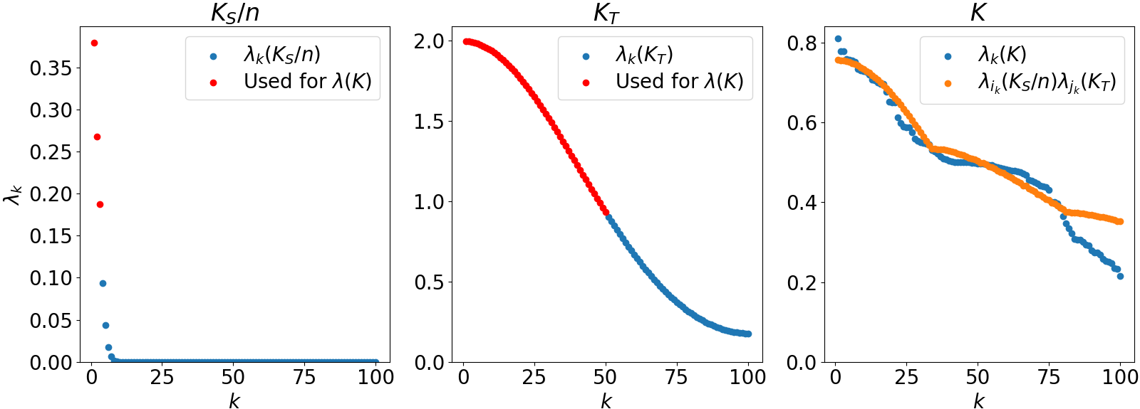
Figure 1: Spectra of $\bm{K}^{(n)}_{S}/n$ (left), $\bm{K}^{(n)}_{T}$ (middle) and $\bm{K}^{(n)}$ (right) when $k_{S}$ and $k_{T}$ are RBF kernels and $n=100$. The spectrum of each kernel matrix is plotted in blue and the approximation (11) of the spectrum of $\bm{K}^{(n)}$ is plotted in orange. The eigenvalues in the spatial (left) and temporal (middle) spectra used in the approximation are colored in red. The spatial component $\bm{x}_{i}$ of an observation $\left(\bm{x}_{i},t_{i},y_{i}\right)$ is collected uniformly in $\mathcal{S}=[0,1]^{d}$ while the temporal component is $t_{i}=i\Delta$.

4 On the Spectrum of the Temporal Kernel Matrix

In this section, we provide the results needed to better understand the spectral properties of temporal kernel matrices $\bm{K}^{(n)}_{T}$ for all major classes of stationary temporal kernels $k_{T}$. We propose a classification of temporal kernels based on properties (boundedness and discreteness) of the support of their associated spectral densities $S_{T}$. Recall that the spectral density $S_{T}$ associated with a stationary kernel $k_{T}$ defined on a unidimensional domain $\mathcal{X}$ is the Fourier transform of $k_{T}$, that is,

$$S_{T}(\omega)=\int_{\mathcal{X}}k_{T}(t)e^{-2\pi it\omega}dt.$$ (12)

More precisely, our classification has four classes and is based on the boundedness and discreteness of the support of $S_{T}$, as listed in the first rows of Table 1 along with an example of kernel that belongs to each class.

4.1 Broadband Kernels

This class comprises the most common kernels in the BO framework, e.g., the Gaussian (RBF) kernel, the Matérn kernel or the rational quadratic kernel. We call them "broadband" because these kernels exploit the whole frequency domain (the support of their spectral densities (12) is continuous and unbounded). We provide an approximation of the spectrum of the temporal covariance matrix built with a broadband kernel.

Proposition 4.1.

Let $\mathcal{D}_{n}=\left\{(\bm{x}_{i},t_{i},y_{i})\right\}_{i\in[n]}$ be a dataset of $n$ observations where $\forall i\in[n],t_{i}=i\Delta$ and let $\bm{K}_{T}^{(n)}=k_{T}(\mathcal{D}_{n},\mathcal{D}_{n})$. If $k_{T}$ has a spectral density supported on a (potentially unbounded) continuous interval, then for all $i\in[n]$,

$$\lambda_{i}\left(\bm{K}^{(n)}_{T}\right)\approx\frac{1}{\Delta}S_{T}\left(\frac{i-n/2}{n\Delta}\right),$$ (13)

where $S_{T}$ is the spectral density associated with $k_{T}$. Equality is achieved when $n\to\infty$.

From Proposition 4.1, proven in Appendix D, we see that the eigenvalues of $\bm{K}^{(n)}_{T}$ sample $S_{T}$ in the interval $I=[-1/2\Delta,1/2\Delta]$. We can therefore deduce that (i) increasing the observation sampling frequency (i.e., reducing $\Delta$) increases the size of $I$ and (ii) increasing the number of observations $n$ does not affect $I$ but refines the granularity of the sampling of $S_{T}$ on $I$. Figure 2 illustrates both points (i) and (ii) experimentally when $k_{T}$ is a Gaussian kernel. In this case, $S_{T}$ is also a Gaussian function, which explains the shape drawn by the orange dots in Figure 2. When $1/\Delta$ is doubled (middle panel in Figure 2), $S_{T}$ is sampled on an interval twice as large. However, when $n$ doubles (right panel in Figure 2), $S_{T}$ is sampled with a granularity twice as high. These insights explain the behavior of the spectrum of $\bm{K}^{(n)}_{T}$ and the Gaussian shape observed in the middle panel of Figure 1.

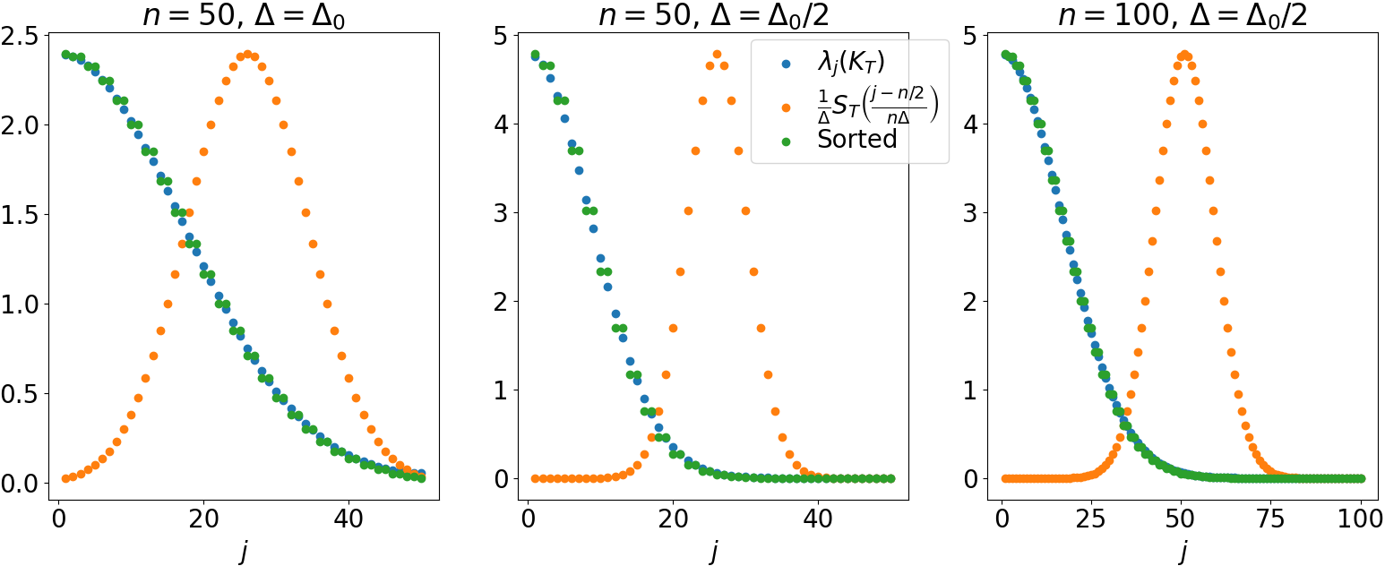
Figure 2: Spectrum of the temporal kernel matrix $\bm{K}_{T}^{(n)}$ (blue) and its approximation (13) with the eigenvalues sorted (green) for different number of observations $n$, different sampling frequencies $\Delta$ and with $k_{T}$ being an RBF kernel. The unsorted spectrum approximation (13) is in orange.

4.2 Band-Limited Kernels

These kernels exploit only a compact subinterval of the frequency domain, as the supports of their spectral densities are continuous and bounded, i.e., $\operatorname*{supp}(S_{T})=[-\tau,\tau]$. We call them "band-limited" by opposition to "broadband" kernels and similarly to the well-known notion of band-limitedness in signal processing. The most popular band-limited kernel is certainly the sinc kernel tobar2019band which is used to fit a GP to a band-limited signal.

Proposition 3.3 also holds for band-limited kernels, as discussed in Appendix D. Consequently, all the observations made for broadband kernels in Section 4.1 can also be made for band-limited kernels. Furthermore, using Proposition 4.1 in conjunction with $\operatorname*{supp}(S_{T})=[-\tau,\tau]$ suggests the existence of a critical sampling frequency above which some eigenvalues of $\bm{K}^{(n)}_{T}$ are 0. More precisely, simple reasoning shows that (i) some eigenvalues are 0 when $1/\Delta>2\tau$ and that (ii) the number of positive eigenvalues in the spectrum of $\bm{K}^{(n)}_{T}$ is $n\min(1,2\tau\Delta)$. These two observations relate to well-known notions in signal processing: (i) is precisely the Nyquist rate derived in the Nyquist sampling theorem nyquist1928certain and (ii) is an instance of the time-bandwidth product landau1961prolate .

Observations (i) and (ii) are illustrated empirically in Figure 3, generated with $k_{T}$ being a sinc2 kernel. The Fourier transform of a sinc2 function is the triangle function, which can be seen in orange in Figure 3. As predicted, sampling observations above the Nyquist rate $2\tau$ (see the middle and right panels in Figure 3) yields eigenvalues that are $0$.

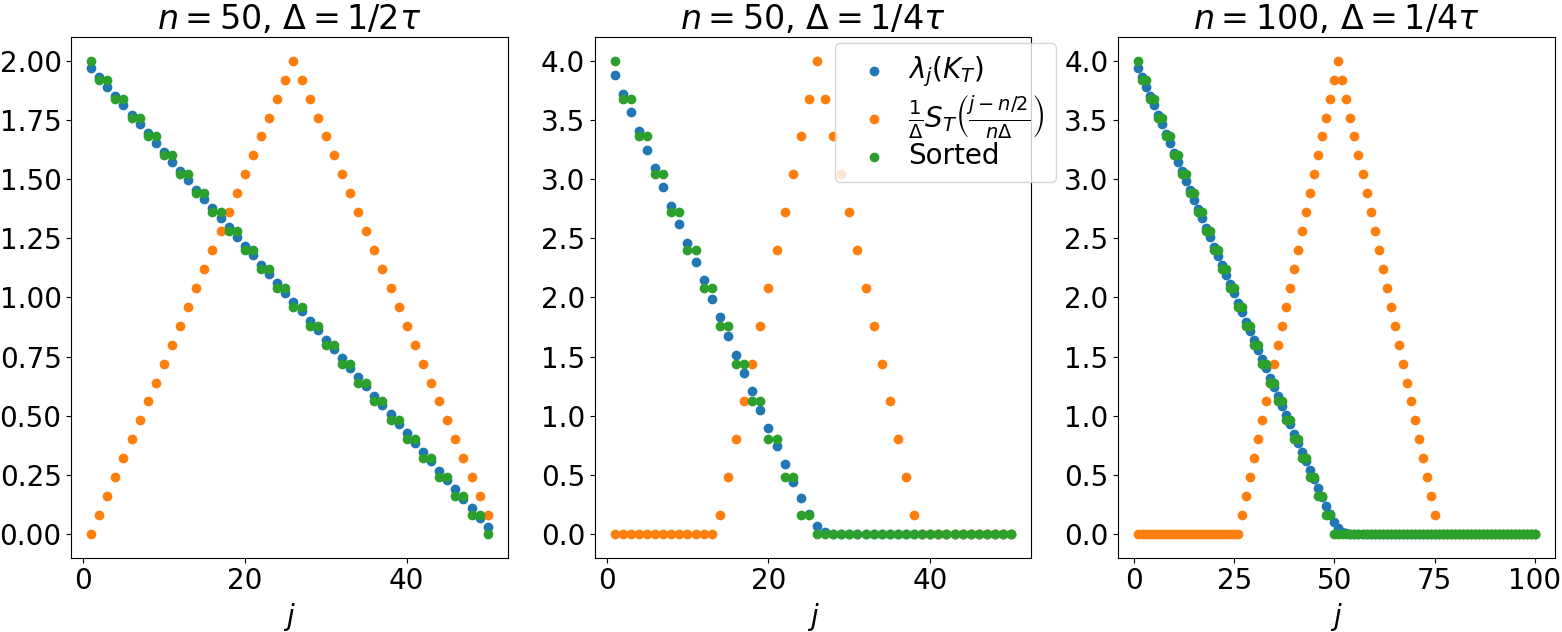
Figure 3: Spectrum of the temporal kernel matrix $\bm{K}_{T}^{(n)}$ (blue) and its approximation (13) with the eigenvalues sorted (green) for different number of observations $n$, different sampling frequencies $\Delta$ and with $k_{T}$ being an sinc2 kernel. The unsorted spectrum approximation (13) is in orange.

4.3 Almost-Periodic Kernels

This class comprises all kernels whose spectral densities are supported on discrete sets of infinite cardinality. In other words, a kernel $k_{T}$ belonging to this class has a spectral density $S_{T}$ that is an infinite mixture of Dirac deltas, that is, $S_{T}(\omega)=\sum_{p\in\mathbb{Z}}\alpha_{p}\delta(\omega-\omega_{p})$, where $\alpha_{-p}=\alpha_{p}$ and $\omega_{-p}=-\omega_{p}$ for all $p\in\mathbb{N}$ to ensure that $k_{T}$ is even and real. We call these kernels "almost-periodic" since they match the definition of almost-periodic functions, introduced by bohr1926theorie . The designation is standard in harmonic analysis. The most popular kernel in this class is undoubtedly the periodic kernel mackay1998introduction , which is widely used to produce a GP surrogate of a function that exactly repeats itself after some time.

Analyzing the spectrum of $\bm{K}^{(n)}_{T}$ built with an almost-periodic kernel is difficult. To simplify this analysis, we introduce the following result.

Proposition 4.2.

Let $k_{T}$ be an almost-periodic kernel. For any $\epsilon>0$, there exists a low-rank kernel $\tilde{k}_{T}^{(\epsilon)}$ such that, for any $i,j\in\mathbb{N}$,

$$\left|k_{T}(t_{i},t_{j})-\tilde{k}^{(\epsilon)}_{T}(t_{i},t_{j})\right|\leq\epsilon.$$ (14)

Proposition 4.2 is proven in Appendix E. It states that any almost-periodic kernel can be approximated arbitrarily well by a kernel $\tilde{k}_{T}$ that is low-rank, whose properties are studied in Section 4.4.

Periodic Kernel with Commensurate Sampling Frequency. The periodic kernel is by far the most popular kernel in this class. Let us briefly illustrate Proposition 4.2 with a simple but important example, where $k_{T}$ is a periodic kernel of period $r$ and where $\Delta$ is commensurate to the period, i.e., $\Delta=r/k$ for some $k\in\mathbb{N}^{+}$. A low-rank kernel $\tilde{k}_{T}$ that perfectly interpolates the points $\left\{k_{T}(j\Delta)\right\}_{j\in[0,n-1]}$ is $\tilde{k}_{T}(j\Delta)=\sum_{i=0}^{n-1}c_{i}\cos(2\pi ij/n)$, with $c_{0}=\sum_{j=0}^{n-1}k_{T}(j\Delta)/n$ and $c_{i}=2\sum_{j=0}^{n-1}k_{T}(j\Delta)\cos(2\pi ij/n)/n$ for all $1\leq i\leq n-1$. The coefficients $c_{i},0\leq i<n$, are obtained by taking the Discrete Cosine Transform (DCT) of the sequence $\left\{k_{T}(j\Delta)\right\}_{j\in[0,n-1]}$. Because $k_{T}$ is periodic with period $r$ and $\Delta=r/k$, a simple analysis shows that for any $n>k$, $c_{0}$ is positive if $k$ is odd and $0$ if $k$ is even. Furthermore, only $\lfloor k/2\rfloor$ coefficients among $c_{1},\cdots,c_{n-1}$ are positive. In other words, the sequence $\left\{k_{T}(j\Delta)\right\}_{j\in[0,n-1]}$ can always be perfectly reconstructed using a sum of at most $\lfloor k/2\rfloor$ cosines and a constant term. Proposition 4.3, stated in the next section, predicts that the spectrum of the temporal kernel matrix $\bm{K}^{(n)}_{T}$ built with a periodic kernel of period $r$ on observations sampled at frequency $k/r$ has at most $k$ positive eigenvalues. This is illustrated experimentally by Figure 4, which shows that $\bm{K}^{(n)}_{T}$ has only 3 (resp., 6) positive eigenvalues when $\Delta=r/3$ (resp., $\Delta=r/6$).

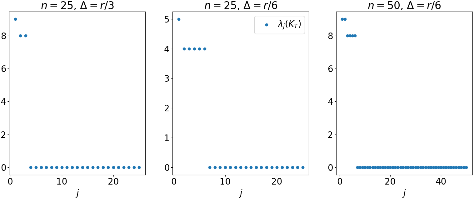
Figure 4: Spectrum of the temporal empirical kernel matrix $\bm{K}_{T}^{(n)}$ for a periodic kernel of period $r$, two commensurate sampling frequencies ($3/r$ and $6/r$) and two different number of observations.

4.4 Low-Rank Kernels

These kernels are trigonometric polynomials, and their spectral densities are supported on discrete sets of finite cardinality. In other words, a kernel $k_{T}$ belonging to this class has a spectral density which is a finite mixture of Dirac deltas, that is, $S_{T}(\omega)=\sum_{p=-L}^{L}\alpha_{p}\delta(\omega-\omega_{p})$, where $\alpha_{-p}=\alpha_{p}$ and $\omega_{p}=\omega_{-p}$ for all $p\in\left\{0,\cdots,L\right\}$, to ensure that $k_{T}$ is even and real. The most popular use of these kernels is definitely random features approximation (e.g., see rahimi2007random ). The following result provides an approximation of the eigenvalues of $\bm{K}^{(n)}_{T}$ when $k_{T}$ is a low-rank kernel.

Proposition 4.3.

Let $\mathcal{D}_{n}=\left\{(\bm{x}_{i},t_{i},y_{i})\right\}_{i\in[n]}$ be a dataset of $n$ observations where, for all $i\in[n],t_{i}=i\Delta$ and let $\bm{K}_{T}^{(n)}=k_{T}(\mathcal{D}_{n},\mathcal{D}_{n})$. If the spectral density $S_{T}$ is supported on a finite discrete set, then there exist $L\in\mathbb{N}$, frequencies $\omega_{1},\cdots,\omega_{L}\in\mathbb{R}$ and positive coefficients $c_{0},\cdots,c_{L}\in[0,1]$ such that $\sum_{j=0}^{L}c_{j}=1$ and $k_{T}(t-t^{\prime})=c_{0}+\sum_{j=1}^{L}c_{j}\cos(2\pi i\omega_{j}|t-t^{\prime}|)$. Furthermore,

$$\lambda_{j}\left(\bm{K}^{(n)}_{T}\right)\approx\begin{cases}nc_{0}&\text{if }j=1,\\ \frac{n}{2}c_{\lfloor j/2\rfloor}&\text{if }2\leq j\leq 2L+1,\\ 0&\text{otherwise}.\end{cases}$$ (15)

Equality is achieved when $n\to+\infty$.

Proposition 4.3 is proven in Appendix E. It states that low-rank kernels whose spectral density is a mixture of $2L+1$ Dirac deltas produce temporal covariance matrices $\bm{K}^{(n)}_{T}$ with at most $2L+1$ eigenvalues. This is the reason why we call these kernels "low-rank".

5 Asymptotic Guarantees for TVBO

The results in Section 4 provide approximations for the spectrum of $\bm{K}^{(n)}_{T}$ for all major classes of kernels. We now use these results in conjunction with Theorems 3.1 and 3.2 to bound the cumulative regrets of TVBO algorithms. Our main results are summarized in Table 1.

Theorem 5.1.

Let $R_{n}=\sum_{i=1}^{n}f(\bm{x}^{*}_{i},t_{i})-f(\bm{x}_{i},t_{i})$ be the cumulative regret incurred by a TVBO algorithm $\mathcal{A}$ at time $t_{n}$, where $\bm{x}^{*}_{n}=\operatorname*{arg\,max}_{\bm{x}\in\mathcal{S}}f(\bm{x},t_{n})$, $\bm{x}_{n}=\operatorname*{arg\,max}_{\bm{x}\in\mathcal{S}}\varphi_{n-1}(\bm{x},t_{n})$. Then,

1. if $k_{T}$ is a broadband or a band-limited kernel, $\mathbb{E}\left[R_{n}\right]\in\Theta(n)$,

2. if $k_{T}$ is an almost-periodic or a low-rank kernel and $\varphi_{n-1}$ is GP-UCB gpucb , $\mathcal{A}$ has the no-regret property, i.e., $\lim_{n\to\infty}R_{n}/n=0$ with high probability.

Theorem 5.1 is proven in Appendix F. To prove (i) (resp., (ii)), we use Proposition 4.1 (resp., Propositions 4.2 and 4.3) to show that, when $\operatorname*{supp}(S_{T})$ is continuous (resp., discrete), the number of eigenvalues of $\bm{K}^{(n)}$ comprised in an arbitrary interval $[a,b]$ scales (resp., remains constant) with the number of observations $n$, as reported in Table 1. This can directly be used in conjunction with Theorem 3.2 (resp., Theorem 3.1) to show that the cumulative regret of any TVBO algorithm that uses a broadband or a band-limited (resp., an almost-periodic or a low-rank) temporal kernel scales linearly with $n$ (resp., has the no-regret property).

Figure 5 illustrates these findings empirically. The left panel shows that the number of eigenvalues in a fixed interval $[a,b]$ when using a broadband or a band-limited temporal kernel scales with $n$, but remains constant for an almost-periodic or a low-rank kernel. The mutual information $I(\bm{f}_{n},\bm{y}_{n})$ shows a similar scaling with $n$ (see the right panel). Recall that if $I(\bm{f}_{n},\bm{y}_{n})\in\mathcal{O}(n)$, the upper regret bound provided by Theorem 3.1 is linear.

Because most time-varying problems require a broadband or a band-limited temporal kernel, Theorem 5.1 has important implications in practice. In particular, it establishes that for most problems, it is hopeless to look for a new acquisition function or an adequate value of $\Delta$ so that a TVBO algorithm can perfectly track the maximizer of $f$ through time. Intuitively, there is always something new to learn each time the objective function is observed. In contrast, when the values of $f$ have a simple enough temporal correlation structure (e.g., $f$ is periodic in the temporal dimension) we can hope for the TVBO algorithm to eventually perfectly track $\operatorname*{arg\,max}_{\bm{x}\in\mathcal{S}}f(\bm{x},t)$ through time.

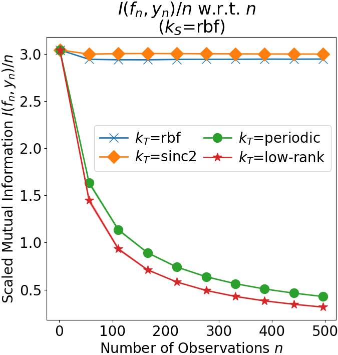
Figure 5: (Left) Number of eigenvalues in the spectrum of $\bm{K}^{(n)}$ in a given interval $[a,b]$, where $a=1$ and $b=2$, w.r.t. the number of observations $n$. (Right) Mutual information (see (7)) scaled by $n$ w.r.t. $n$. Both plots use four different temporal kernels, namely an RBF kernel (blue crosses), a sinc2 kernel (orange diamonds), a periodic kernel (green circles) and a low-rank kernel (red stars). The spatial components of observations are collected uniformly in $\mathcal{S}=[0,1]^{d}$ while the temporal components follow Assumption 2.3. The results are averaged over 10 replications and standard error intervals are plotted as shaded areas around the solid lines.

6 Conclusion

This paper solves an important theoretical question about the asymptotic performance of TVBO algorithms opened almost ten years ago with the first derivation of an algorithm-independent lower regret bound in bogunovic2016time . Under mild assumptions (see Section 2.3) and for the most popular classes of stationary temporal kernels, we have provided an algorithm-independent lower regret bound (Theorem 3.2) and an upper regret bound (Theorem 3.1), and we have established an important connection between the support of the spectral density associated with the temporal kernel $k_{T}$ and the asymptotic guarantees that can be provided by the TVBO framework, as summarized by Theorem 5.1 and Table 1. Finally, we have illustrated each important theoretical result experimentally (see Figures 1-5).

This work also opens up new research questions. How is the cumulative regret $R_{n}$ evolving when $k_{T}$ is a combination of temporal kernels that come from different classes (e.g., a low-rank kernel and a band-limited kernel)? What is the asymptotical performance of TVBO algorithms for more complex spatio-temporal covariance structures (e.g., by relaxing Assumption 2.2)? How does $R_{n}$ evolve when observations are not sampled at a fixed sampling frequency (i.e., when Assumption 2.3 is relaxed)? These questions have both theoretical and practical interest. As an example, there are numerous applications in which a new observation is sampled only after performing GP inference. As the complexity of GP inference is in $\mathcal{O}(n^{3})$, observations may not be collected at a fixed sample frequency bardou2024too , and studying $R_{n}$ without Assumption 2.3 appears to be crucial for improving TVBO algorithms in practice. Addressing these questions would deepen our understanding of TVBO algorithms and lead to significant improvements in their empirical performance. The tools and insights provided by this paper will likely help the TVBO community to come up with answers on these important questions.

Appendix A Upper Cumulative Regret Bound for GP-UCB-Based TVBO Algorithms

In this appendix, we provide all the details required to prove Theorem 3.1. For the sake of completeness, we start by deriving the usual instantaneous regret bound provided in most regret proofs that involve GP-UCB [4, 7].

Lemma A.1.

Let $r_{n}=f(\bm{x}^{*}_{n},t_{n})-f(\bm{x}_{n},t_{n})$ be the instantaneous regret at the $n$-th iteration of the TVBO algorithm, where $\bm{x}^{*}_{n}=\operatorname*{arg\,max}_{\bm{x}\in\mathcal{S}}f(\bm{x},t_{n})$, $\bm{x}_{n}=\operatorname*{arg\,max}_{\bm{x}\in\mathcal{S}}\varphi_{n-1}(\bm{x},t_{n})$ and where $\varphi_{n-1}$ is GP-UCB. Pick $\delta>0$, then with probability at least $1-\delta$,

$$r_{n}\leq 2\beta_{n}^{1/2}\sigma_{n-1}(\bm{x}_{n},t_{n})+\frac{1}{n^{2}}$$ (16)

where $\sigma_{n-1}(\bm{x},t_{n})$ is the standard deviation of the GP conditioned on $n-1$ observations and where

$$\beta_{n}=2d\log\left(Ldn^{2}/6\delta\right)+4\log(\pi n).$$ (17)

Proof.

For the sake of consistency with the literature we reuse, whenever appropriate, the notations in [7]. Let us set a discretization $\mathcal{S}_{n}$ of the spatial domain $\mathcal{S}\subseteq[0,1]^{d}$. $\mathcal{S}_{n}$ is of size $\tau_{n}^{d}$ and satisfies

$$||\bm{x}-[\bm{x}]_{n}||_{1}\leq\frac{d}{\tau_{n}},\text{ }\forall\bm{x}\in\mathcal{S},$$ (18)

where $[\bm{x}]_{n}=\operatorname*{arg\,min}_{\bm{s}\in\mathcal{S}_{n}}||\bm{s}-\bm{x}||_{1}$ is the closest point in $\mathcal{S}_{n}$ to $\bm{x}$ according to the $L^{1}$-norm. Note that a uniform grid on $\mathcal{S}$ ensures (18).

Let us now fix $\delta>0$ and condition on a high-probability event. If $\beta_{n}=2\log\frac{\tau_{n}^{d}\pi^{2}n^{2}}{6\delta}$, then

$$|f(\bm{x},t_{n})-\mu_{n-1}(\bm{x},t_{n})|\leq\beta_{n}^{1/2}\sigma_{n-1}(\bm{x},t_{n}),\text{ }\forall n\in\mathbb{N},\forall\bm{x}\in\mathcal{S}_{n}$$ (19)

with probability at least $1-\delta$. This directly comes from $f(\bm{x},t_{n})\sim\mathcal{N}\left(\mu_{n-1}(\bm{x},t_{n}),\sigma_{n-1}^{2}(\bm{x},t_{n})\right)$ and from the Chernoff concentration inequality applied to Gaussian tails $\mathbb{P}\left(|f(\bm{x},t_{n})-\mu_{n-1}(\bm{x},t_{n})|\leq\sqrt{\beta_{n}}\sigma_{n-1}(\bm{x},t_{n})\right)\geq 1-e^{-\beta_{n}/2}$. Therefore, our choice of $\beta_{n}$ ensures that for a given $n$ and a given $\bm{x}\in\mathcal{S}_{n}$, $|f(\bm{x},t_{n})-\mu_{n-1}(\bm{x},t_{n})|\leq\beta_{n}^{1/2}\sigma_{n-1}(\bm{x},t_{n})$ occurs with a probability at least $1-\frac{6\delta}{\pi^{2}n^{2}\tau_{n}^{d}}$. The union bound taken over $n\in\mathbb{N}$ and $\bm{x}\in\mathcal{S}_{n}$ establishes (19) with probability $1-\delta$.

Recall that Assumption 2.4 ensures that for all $\bm{x}\in\mathcal{S}$ and all $t_{n}\in\mathcal{T}$,

$$|f(\bm{x},t_{n})-f([\bm{x}]_{n},t_{n})| \leq L||\bm{x}-[\bm{x}]_{n}||_{1}$$

$$\leq\frac{Ld}{\tau_{n}},$$ (20)

where (20) comes from (18).

Therefore, setting $\tau_{n}=Ldn^{2}$ yields that for all $\bm{x}\in\mathcal{S}$ and all $t_{n}\in\mathcal{T}$,

$$|f(\bm{x},t_{n})-f([\bm{x}]_{n},t_{n})|\leq\frac{1}{n^{2}}.$$ (21)

Because $\tau_{n}=Ldn^{2}$, $\beta_{n}$ becomes $2d\log\left(Ldn^{2}/6\delta\right)+4\log(\pi n)$. Using the triangle inequality and combining (19) with (21), we get that $\bm{x}^{*}_{n}=\operatorname*{arg\,max}_{\bm{x}\in\mathcal{S}}f(\bm{x},t_{n})$ satisfies

$$|f(\bm{x}^{*}_{n},t_{n})-\mu_{n-1}([\bm{x}^{*}_{n}]_{n},t_{n})| \leq|f([\bm{x}^{*}_{n}]_{n},t_{n})-\mu_{n-1}([\bm{x}^{*}_{n}]_{n},t_{n})|+|f(\bm{x}^{*}_{n},t_{n})-f([\bm{x}^{*}_{n}]_{n},t_{n})|$$

$$\leq\beta_{n}^{1/2}\sigma_{n-1}([\bm{x}^{*}_{n}]_{n},t_{n})+\frac{1}{n^{2}}.$$ (22)

We can now bound the instantaneous regret of the TVBO algorithm from above:

$$r_{n} =f(\bm{x}^{*}_{n},t_{n})-f(\bm{x}_{n},t_{n})$$

$$\leq\mu_{n-1}([\bm{x}^{*}_{n}]_{n},t_{n})+\beta_{n}^{1/2}\sigma_{n-1}([\bm{x}^{*}_{n}]_{n},t_{n})+\frac{1}{n^{2}}-f(\bm{x}_{n},t_{n})$$ (23)

$$\leq\mu_{n-1}(\bm{x}_{n},t_{n})+\beta_{n}^{1/2}\sigma_{n-1}(\bm{x}_{n},t_{n})+\frac{1}{n^{2}}-f(\bm{x}_{n},t_{n})$$ (24)

$$\leq 2\beta_{n}^{1/2}\sigma_{n-1}(\bm{x}_{n},t_{n})+\frac{1}{n^{2}},$$ (25)

where (23) follows directly from (22), (24) from the definition of $\bm{x}_{n}=\operatorname*{arg\,max}_{\bm{x}\in\mathcal{S}}\varphi_{n-1}(\bm{x},t_{n})=\operatorname*{arg\,max}_{\bm{x}\in\mathcal{S}}\mu_{n-1}(\bm{x},t_{n})+\beta_{n}^{1/2}\sigma_{n-1}(\bm{x},t_{n})$ and (25) from (19). ∎

Lemma A.1 shows that the posterior standard deviation of the surrogate GP plays a key role in the regret bound. Based on an original idea from [4], let us now connect the cumulative regret $R_{n}=\sum_{i=1}^{n}r_{i}$ to $I(\bm{f}_{n},\bm{y}_{n})$, the mutual information between the random vector $\bm{f}_{n}=\left(f(\bm{x}_{1},t_{1}),\cdots,f(\bm{x}_{n},t_{n})\right)$ and $\bm{y}_{n}=\left(y_{1},\cdots,y_{n}\right)$.

Lemma A.2.

Let $r_{n}$ be the instantaneous regret of a TVBO algorithm using the GP-UCB acquisition function. Pick $\delta\in[0,1]$. Then, with probability $1-\delta$,

$$R_{n}\leq\sqrt{8C_{1}\beta_{n}\sigma^{2}_{0}nI(\bm{f}_{n},\bm{y}_{n})}+\frac{\pi^{2}}{6}$$ (26)

where

$$I(\bm{f}_{n},\bm{y}_{n})=\frac{1}{2}\sum_{i=1}^{n}\log(1+\sigma_{0}^{-2}\sigma_{i-1}^{2}(\bm{x}_{i},t_{i})).$$ (27)

Proof.

We have the following:

$$R_{n} =\sum_{i=1}^{n}r_{i}$$

$$\leq\sum_{i=1}^{n}2\beta_{i}^{1/2}\sigma_{i-1}(\bm{x}_{i},t_{i})+\frac{1}{i^{2}}$$ (28)

$$\leq\sqrt{n\sum_{i=1}^{n}4\beta_{i}\sigma_{i-1}^{2}(\bm{x}_{i},t_{i})}+\frac{\pi^{2}}{6}$$ (29)

$$\leq\sqrt{4n\beta_{n}\sigma_{0}^{2}\sum_{i=1}^{n}\sigma_{0}^{-2}\sigma_{i-1}^{2}(\bm{x}_{i},t_{i})}+\frac{\pi^{2}}{6}$$ (30)

$$\leq\sqrt{4nC_{1}\beta_{n}\sigma_{0}^{2}\sum_{i=1}^{n}\log(1+\sigma_{0}^{-2}\sigma_{i-1}^{2}(\bm{x}_{i},t_{i})})+\frac{\pi^{2}}{6},$$ (31)

where (28) is a direct application of Lemma A.1, (29) is a direct application of the Cauchy-Schwarz inequality and the solution to the Basel problem, (30) holds because $\left\{\beta_{n}\right\}_{n\in\mathbb{N}}$ is an increasing sequence (see (17)) and where (31) holds because for $C_{1}=\sigma^{-2}_{0}/\log(1+\sigma^{-2}_{0})$ and for any $z\in\left[0,\sigma_{0}\right]$, $z^{2}\leq C_{1}\log(1+z^{2})$.

In (31), we recognize the expression of the mutual information $I(\bm{f}_{n},\bm{y}_{n})$ given in [4] and in (27) for the sake of completeness. Together, (27) and (31) completes the proof. ∎

Finally, we introduce an approximation of the mutual information (27) that involves the spectral properties of the covariance operator $\Sigma_{k}$.

Lemma A.3.

Let $I(\bm{f}_{n},\bm{y}_{n})$ be the mutual information between the random vector $\bm{f}_{n}=\left(f(\bm{x}_{1},t_{1}),\cdots,f(\bm{x}_{n},t_{n})\right)$ and $\bm{y}_{n}=\left(y_{1},\cdots,y_{n}\right)$. Then,

$$I(\bm{f}_{n},\bm{y}_{n})\approx\frac{1}{2}\sum_{i=1}^{n}\log(1+\sigma^{-2}_{0}n\bar{\lambda}_{i})$$

where $\bar{\lambda}_{i}$ is the $i$-th largest eigenvalue of the covariance operator $\Sigma_{k}$ (see (3)). Equality is achieved when $n\to\infty$.

Proof.

The proof is immediate by recalling the alternative form of the mutual information $I(\bm{f}_{n},\bm{y}_{n})=\frac{1}{2}\log\det(\bm{I}+\sigma^{-2}_{0}\bm{K}^{(n)})$, where $\bm{I}$ is the $n\times n$ identity matrix. Therefore we have

$$I(\bm{f}_{n},\bm{y}_{n}) =\frac{1}{2}\log\det\left(\bm{I}+\sigma^{-2}_{0}\bm{K}^{(n)}\right)$$

$$=\frac{1}{2}\log\prod_{i=1}^{n}\lambda_{i}\left(\bm{I}+\sigma^{-2}_{0}\bm{K}^{(n)}\right)$$ (32)

$$=\frac{1}{2}\sum_{i=1}^{n}\log\lambda_{i}\left(\bm{I}+\sigma^{-2}_{0}\bm{K}^{(n)}\right)$$ (33)

$$=\frac{1}{2}\sum_{i=1}^{n}\log\left(1+\sigma^{-2}_{0}\lambda_{i}\left(\bm{K}^{(n)}\right)\right)$$

$$\approx\frac{1}{2}\sum_{i=1}^{n}\log\left(1+\sigma^{-2}_{0}n\bar{\lambda}_{i}\right),$$ (34)

where (32) holds because the determinant of any matrix is equal to the product of its eigenvalues, (33) holds because of the product rule of the logarithm and where (34) comes from the connection between the spectrum of the covariance operator $\Sigma_{k}$ and the spectrum of the covariance matrix $\bm{K}^{(n)}$ (see (4)). ∎

Together, Lemmas A.1, A.2 and A.3 yield Theorem 3.1.

Appendix B Algorithm-Independent Lower Cumulative Regret Bound

In this appendix, we prove Theorem 3.2, which provides a generic algorithm-independent lower bound on the cumulative regret $R_{n}$ of a TVBO algorithm using spectral properties of covariance operator $\Sigma_{k}$ associated with $k$. Because we seek an algorithm-independent lower bound for the cumulative regret $R_{n}$, we can assume an arbitrarily small observational noise $\sigma^{2}_{0}$, as long as $\sigma^{2}_{0}$ remains nonnegative. For the exact same reason, we can also assume an arbitrarily high sampling frequency $1/\Delta$ as long as it remains finite (i.e., $1/\Delta<\infty$ or, equivalently, $\Delta>0$).

Access to the true objective function. In TVBO, $f$ is a posterior GP that serves as a surrogate model for the true, unknown objective function $\bar{f}$ observed at each iteration. On the one hand, $f$ is a GP that defines a probability distribution on the Reproducing Kernel Hilbert Space (RKHS) of $k$. Its maximal argument at time $t_{n}$ is the random variable $\bm{x}^{*}_{n}=\operatorname*{arg\,max}_{\bm{x}\in\mathcal{S}}f(\bm{x},t_{n})$. On the other hand, $\bar{f}$ is the deterministic function in the RKHS of $k$ that the TVBO algorithm would like to maximize. Its maximal argument at time $t_{n}$ is the deterministic value $\bar{\bm{x}}^{*}_{n}=\operatorname*{arg\,max}_{\bm{x}\in\mathcal{S}}\bar{f}(\bm{x},t_{n})$. In the following, we use $\bar{\bm{x}}^{*}_{n}$ to bound $R_{n}$ from below.

Let us start with the following lemma.

Lemma B.1.

Let $\mu_{n}(\bm{x},t)$ and $\sigma^{2}_{n}(\bm{x},t)$ be the posterior mean and variance of $f(\bm{x},t)$ after observing $\mathcal{D}_{n}=\left\{(\bm{x}_{i},t_{i},\bar{f}(\bm{x}_{i},t_{i})\right\}_{i\in[n]}$. Then,

$$\mu_{n}(\bm{x},t) \approx\frac{1}{n}\sum_{i=1}^{n}\bar{\phi}_{i}(\bm{x},t)\sum_{j=1}^{n}\bar{\phi}_{i}(\bm{x}_{j},t_{j})\bar{f}(\bm{x}_{j},t_{j})$$ (35)

$$\sigma^{2}_{n}(\bm{x},t) \approx 1-\sum_{i=1}^{n}\bar{\lambda}_{i}\bar{\phi}^{2}_{i}(\bm{x},t),$$ (36)

where $\left\{\bar{\lambda}_{i}\right\}_{i\in\mathbb{N}}$ are the eigenvalues of $\Sigma_{k}$, the covariance operator associated with $k$ (see (3)), and where $\left\{\bar{\phi}_{i}\right\}_{i\in\mathbb{N}}$ are the corresponding eigenfunctions of $\Sigma_{k}$. Equality is achieved when $n\to+\infty$.

Proof.

Let us start by recalling that any positive-definite, stationary kernel $k:\mathcal{X}^{2}\to\mathbb{R}$ admits a Mercer decomposition [21] that uses the eigenvalues $\left\{\bar{\lambda}_{i}\right\}_{i\in\mathbb{N}}$ and eigenfunctions $\left\{\bar{\phi}_{i}\right\}_{i\in\mathbb{N}}$ of its associated covariance operator $\Sigma_{k}$. Furthermore, recall that $\bm{K}^{(n)}$ is a positive semi-definite matrix. Therefore, it admits the spectral decomposition $\bm{K}^{(n)}=\bm{\Phi}^{(n)}\bm{\Lambda}^{(n)}\left(\bm{\Phi}^{(n)}\right)^{\top}$, where $\bm{\Phi}^{(n)}=\left(\bm{\Phi}_{1},\cdots,\bm{\Phi}_{n}\right)$ is the orthogonal matrix whose columns are the eigenvectors of $\bm{K}^{(n)}$ and $\bm{\Lambda}^{(n)}=\text{diag}\left(\Lambda_{1},\cdots,\Lambda_{n}\right)$ is the diagonal matrix whose diagonal entries are the (nonnegative) eigenvalues of $\bm{K}^{(n)}$. Finally, recall the connection between the spectral properties of $\bm{K}^{(n)}$ and the covariance operator $\Sigma_{k}$, that is, $\Lambda_{i}\approx n\bar{\lambda}_{i}$ and $\sqrt{n}\Phi_{ij}\approx\bar{\phi}_{i}(\bm{x}_{j},t_{j})$ for $n$ large enough (see [10]).

Regarding the posterior mean of a GP (given by (1)) and assuming a noiseless setting (i.e., $\sigma^{2}_{0}=0$), we have

$$\mu_{n}(\bm{x},t) =k^{\top}((\bm{x},t),\mathcal{D}_{n})\left(\bm{K}^{(n)}\right)^{-1}\bar{f}(\mathcal{D}_{n})$$

$$=k^{\top}((\bm{x},t),\mathcal{D}_{n})\bm{\Phi}^{(n)}\left(\bm{\Lambda}^{(n)}\right)^{-1}\left(\bm{\Phi}^{(n)}\right)^{\top}\bar{f}(\mathcal{D}_{n})$$ (37)

$$=\sum_{i,j,l=1}^{n}k((\bm{x},t),(\bm{x}_{j},t_{j}))\Phi_{ij}\frac{1}{\Lambda_{i}}\Phi_{il}\bar{f}(\bm{x}_{l},t_{l})$$ (38)

$$=\sum_{i,j,l=1}^{n}\frac{1}{\Lambda_{i}}\Phi_{ij}\Phi_{il}\bar{f}(\bm{x}_{l},t_{l})\sum_{m=1}^{\infty}\bar{\lambda}_{m}\bar{\phi}_{m}(\bm{x},t)\bar{\phi}_{m}(\bm{x}_{j},t_{j})$$ (39)

$$\approx\sum_{i,j,l=1}^{n}\frac{1}{n\bar{\lambda}_{i}}\Phi_{ij}\frac{1}{\sqrt{n}}\bar{\phi}_{i}(\bm{x}_{l},t_{l})\bar{f}(\bm{x}_{l},t_{l})\sum_{m=1}^{n}\bar{\lambda}_{m}\bar{\phi}_{m}(\bm{x},t)\sqrt{n}\Phi_{mj}$$ (40)

$$=\frac{1}{n}\sum_{i,m,l=1}^{n}\frac{\bar{\lambda}_{m}}{\bar{\lambda}_{i}}\bar{\phi}_{m}(\bm{x},t)\bar{\phi}_{i}(\bm{x}_{l},t_{l})\bar{f}(\bm{x}_{l},t_{l})\underbrace{\sum_{j=1}^{n}\Phi_{ij}\Phi_{mj}}_{\delta_{im}}$$ (41)

$$=\frac{1}{n}\sum_{i=1}^{n}\bar{\phi}_{i}(\bm{x},t)\sum_{l=1}^{n}\bar{\phi}_{i}(\bm{x}_{l},t_{l})\bar{f}(\bm{x}_{l},t_{l}),$$ (42)

where $\bar{f}(\mathcal{D}_{n})=\left(\bar{f}(\bm{x}_{1},t_{1}),\cdots,\bar{f}(\bm{x}_{n},t_{n})\right)$, $\delta_{ab}$ is the Kronecker delta with value $1$ if $a=b$ and $0$ otherwise, where (37) uses the spectral decomposition of $\bm{K}^{(n)}$, (38) expresses the matrix products with sums, (39) uses the Mercer decomposition of the kernel $k$, (40) uses the approximation of the eigenvalues and eigenfunctions of $\Sigma_{k}$ that holds when $n$ is large enough, (41) is a simple reordering of terms and where (42) holds because the eigenvectors are orthonormal.

Following a very similar reasoning, we have

$$\sigma^{2}_{n}(\bm{x},t) =1-k^{\top}((\bm{x},t),\mathcal{D}_{n})\left(\bm{K}^{(n)}\right)^{-1}k((\bm{x},t),\mathcal{D}_{n})$$

$$=1-k^{\top}((\bm{x},t),\mathcal{D}_{n})\bm{\Phi}^{(n)}\left(\bm{\Lambda}^{(n)}\right)^{-1}\left(\bm{\Phi}^{(n)}\right)^{\top}k((\bm{x},t),\mathcal{D}_{n})$$ (43)

$$=1-\sum_{i,j,l=1}^{n}k((\bm{x},t),(\bm{x}_{j},t_{j}))\Phi_{ij}\frac{1}{\Lambda_{i}}\Phi_{il}k((\bm{x},t),(\bm{x}_{l},t_{l}))$$ (44)

$$=1-\sum_{i,j,l=1}^{n}\frac{1}{\Lambda_{i}}\Phi_{ij}\Phi_{il}\sum_{m,p=1}^{\infty}\bar{\lambda}_{m}\bar{\lambda}_{p}\bar{\phi}_{m}(\bm{x},t)\bar{\phi}_{m}(\bm{x}_{j},t_{j})\bar{\phi}_{p}(\bm{x},t)\bar{\phi}_{p}(\bm{x}_{l},t_{l})$$ (45)

$$\approx 1-\sum_{i,j,l=1}^{n}\frac{1}{n\bar{\lambda}_{i}}\Phi_{ij}\Phi_{il}\sum_{m,p=1}^{n}\bar{\lambda}_{m}\bar{\lambda}_{p}\bar{\phi}_{l}(\bm{x},t)\bar{\phi}_{p}(\bm{x},t)\sqrt{n}\Phi_{mj}\sqrt{n}\Phi_{pl}$$ (46)

$$=1-\sum_{i,m,p=1}^{n}\frac{\bar{\lambda}_{m}\bar{\lambda}_{p}}{\bar{\lambda}_{i}}\bar{\phi}_{l}(\bm{x},t)\bar{\phi}_{p}(\bm{x},t)\underbrace{\sum_{j=1}^{n}\Phi_{ij}\Phi_{mj}}_{\delta_{im}}\underbrace{\sum_{l=1}^{n}\Phi_{il}\Phi_{pl}}_{\delta_{ip}}$$ (47)

$$=1-\sum_{i=1}^{n}\bar{\lambda}_{i}\bar{\phi}^{2}_{i}(\bm{x},t),$$ (48)

where (43) uses the spectral decomposition of $\bm{K}^{(n)}$, (44) expresses the matrix products with sums, (45) uses the Mercer decomposition of the kernel $k$, (46) uses the approximation of the eigenvalues and eigenfunctions of $\Sigma_{k}$, (47) is a simple reordering of terms and where (48) holds because the eigenvectors are orthonormal. ∎

Lemma B.1 relates the posterior mean and variance of a GP and the spectral properties of the covariance operator $\Sigma_{k}$ associated with $k$. We now proceed to bound the expected instantaneous regret from below.

Lemma B.2.

Let $r_{n}=f(\bm{x}^{*}_{n},t_{n})-f(\bm{x}_{n},t_{n})$ be the instantaneous regret of incurred by a TVBO algorithm at time $t_{n}$, where $\bm{x}^{*}_{{n}}=\operatorname*{arg\,max}_{\bm{x}\in\mathcal{S}}f(\bm{x},t_{n})$ and $\bm{x}_{n}=\operatorname*{arg\,max}_{\bm{x}\in\mathcal{S}}\varphi_{n-1}(\bm{x},t_{n})$. Let $\bar{\bm{x}}^{*}_{n}=\operatorname*{arg\,max}_{\bm{x}\in\mathcal{S}}\bar{f}(\bm{x},t_{n})$. Then,

$$\mathbb{E}\left[r_{n}\right]\geq\hat{\mu}_{n-1}\Phi\left(\frac{\hat{\mu}_{n-1}}{\hat{\sigma}_{n-1}}\right)+\hat{\sigma}_{n-1}\varphi\left(\frac{\hat{\mu}_{n-1}}{\hat{\sigma}_{n-1}}\right),$$ (49)

where

$$\hat{\mu}_{n-1} =\mu_{n-1}(\bar{\bm{x}}^{*}_{{n}},t_{n})-\mu_{n-1}(\bm{x}_{{n}},t_{n}),$$ (50)

$$\hat{\sigma}_{n-1}^{2} =\sigma^{2}_{n-1}(\bar{\bm{x}}_{{n}}^{*},t_{n})+\sigma^{2}_{n-1}(\bm{x}_{{n}},t_{n})+2\mathrm{Cov}_{n-1}\left(\left(\bar{\bm{x}}_{{n}}^{*},t_{n}\right),\left(\bm{x}_{{n}},t_{n}\right)\right),$$ (51)

and where $\Phi$ (resp., $\varphi$) is the c.d.f. (resp., the p.d.f.) of a standard Gaussian distribution.

Proof.

We have

$$r_{{n}} =f(\bm{x}^{*}_{{n}},t_{n})-f(\bm{x}_{{n}},t_{n})$$

$$=\max(0,f(\bm{x}^{*}_{{n}},t_{n})-f(\bm{x}_{{n}},t_{n}))$$ (52)

$$\geq\max(0,f(\bar{\bm{x}}^{*}_{{n}},t_{n})-f(\bm{x}_{{n}},t_{n}))$$ (53)

where (52) comes from $r_{{n}}\geq 0$ because $f(\bm{x}^{*}_{n},t_{n})\geq f(\bm{x},t_{n})$ for all $\bm{x}\in\mathcal{S}$. Equation (53) holds with the same argument since, in particular, $f(\bm{x}^{*}_{{n}},t_{n})\geq f(\bar{\bm{x}}^{*}_{{n}},t_{n})$.

Let us denote by $\hat{r}_{{n}}=\max(0,f(\bar{\bm{x}}^{*}_{{n}},t_{n})-f(\bm{x}_{{n}},t_{n}))$. By definition, $\hat{r}_{{n}}$ follows a (non-normalized) Gaussian distribution $\mathcal{N}\left(\hat{\mu}_{n-1},\hat{\sigma}^{2}_{n-1}\right)$ truncated on $\mathbb{R}^{+}$, where $\hat{\mu}_{n-1}$ and $\hat{\sigma}^{2}_{n-1}$ are given by (50) and (51). The first moment of this distribution is well known:

$$\mathbb{E}\left[\hat{r}_{{n}}\right]=\hat{\mu}_{n-1}\Phi\left(\frac{\hat{\mu}_{n-1}}{\hat{\sigma}_{n-1}}\right)+\hat{\sigma}_{n-1}\varphi\left(\frac{\hat{\mu}_{n-1}}{\hat{\sigma}_{n-1}}\right).$$

Finally, we have $r_{{n}}\geq\hat{r}_{{n}}$ by (53). Therefore, by the monotonicity of expectations, we have $\mathbb{E}[r_{{n}}]\geq\mathbb{E}[\hat{r}_{{n}}]$. This concludes the proof. ∎

Lemma B.2 ensures that a lower bound on $\mathbb{E}[r_{{n}}]$ can be derived by bounding the RHS of (49) from below. A simple analysis shows that such a lower bound can be obtained by plugging in (49) a lower bound for either $\hat{\mu}_{n-1}$ and/or $\hat{\sigma}^{2}_{n-1}$. This is the purpose of the next lemma.

Lemma B.3.

Consider $\hat{\mu}_{n-1}$ and $\hat{\sigma}_{n-1}^{2}$ given by (50) and (51), respectively. Then,

$$\hat{\mu}_{n-1} \approx\frac{1}{n-1}\sum_{i=1}^{n-1}\left(\bar{\phi}_{i}(\bar{\bm{x}}^{*}_{{n}},t_{n})-\bar{\phi}_{i}(\bm{x}_{{n}},t_{n})\right)\sum_{j=1}^{n-1}\bar{\phi}_{i}(\bm{x}_{k},t_{k})\bar{f}(\bm{x}_{k},t_{k}),$$ (54)

$$\hat{\sigma}^{2}_{n-1} \gtrsim 2-\sum_{i=1}^{n-1}\bar{\lambda}_{i}\left(\bar{\phi}^{2}_{i}(\bar{\bm{x}}_{{n}}^{*},t_{n})+\bar{\phi}^{2}_{i}(\bm{x}_{{n}},t_{n})\right),$$ (55)

where $\left\{\bar{\lambda}_{i}\right\}_{i\in\mathbb{N}}$ are the eigenvalues of $\Sigma_{k}$, $\left\{\bar{\phi}_{i}\right\}_{i\in\mathbb{N}}$ are the corresponding eigenfunctions of $\Sigma_{k}$.

Proof.

Let us start by the approximation of (50). We have

$$\hat{\mu}_{n-1} =\mu_{n-1}(\bar{\bm{x}}^{*}_{{n}},t_{n})-\mu_{n-1}(\bm{x}_{{n}},t_{n})$$

$$\approx\frac{1}{n-1}\sum_{i=1}^{n-1}\left(\bar{\phi}_{i}(\bar{\bm{x}}^{*}_{{n}},t_{n})-\bar{\phi}_{i}(\bm{x}_{{n}},t_{n})\right)\sum_{j=1}^{n-1}\bar{\phi}_{i}(\bm{x}_{j},t_{j})\bar{f}(\bm{x}_{j},t_{j})$$ (56)

where (56) follows from a direct application of (35) in Lemma B.1.

Now, let us bound $\hat{\sigma}^{2}_{n-1}$ from below. We have

$$\hat{\sigma}^{2}_{n-1} =\sigma^{2}_{n-1}(\bar{\bm{x}}_{{n}}^{*},t_{n})+\sigma^{2}_{n-1}(\bm{x}_{{n}},t_{n})+2\mathrm{Cov}_{n-1}\left(\left(\bar{\bm{x}}_{{n}}^{*},t_{n}\right),\left(\bm{x}_{{n}},t_{n}\right)\right),$$

$$\geq\sigma^{2}_{n-1}(\bar{\bm{x}}_{{n}}^{*},t_{n})+\sigma^{2}_{n-1}(\bm{x}_{{n}},t_{n}),$$ (57)

$$\approx 2-\sum_{i=1}^{n-1}\bar{\lambda}_{i}\left(\bar{\phi}^{2}_{i}(\bar{\bm{x}}_{{n}}^{*},t_{n})+\bar{\phi}^{2}_{i}(\bm{x}_{{n}},t_{n})\right),$$ (58)

where (57) comes from the covariance being necessarily positive when $\bar{\bm{x}}_{{n}}^{*}$ and $\bm{x}_{{n}}$ are close enough (which is guaranteed when $\Delta$ is small enough and $n$ large enough) and where (58) follows from a direct application of (36) in Lemma B.1. ∎

Combining Lemmas B.1, B.2 and B.3, we get Theorem 3.2.

Appendix C Building the Covariance Operator Spectrum

In this section, we discuss how to build the spectrum of the covariance operator $\Sigma_{k}$ associated with the spatio-temporal kernel $k$ (that is, Proposition 3.3) and the approximation of the empirical covariance matrix spectrum in Corollary 3.4.

We start by proving Proposition 3.3.

Proof.

We have

$$k((\bm{x},t),(\bm{x}^{\prime},t^{\prime})) =k_{S}(\bm{x},\bm{x}^{\prime})k_{T}(t,t^{\prime})$$

$$=\sum_{i=1}^{\infty}\bar{\lambda}^{S}_{i}\bar{\phi}^{S}_{i}(\bm{x})\bar{\phi}^{S}_{i}(\bm{x}^{\prime})\sum_{j=1}^{\infty}\bar{\lambda}^{T}_{j}\bar{\phi}^{T}_{j}(t)\bar{\phi}^{T}_{j}(t^{\prime})$$ (59)

$$=\sum_{i,j=1}^{\infty}\underbrace{\bar{\lambda}^{S}_{i}\bar{\lambda}^{T}_{j}}_{\text{Eigenvalue }\bar{\lambda}_{l}\text{ }}\underbrace{\bar{\phi}^{S}_{i}(\bm{x})\bar{\phi}^{T}_{j}(t)}_{\text{ Eigenfunction }\bar{\phi}_{l}(\bm{x},t)}\bar{\phi}^{S}_{i}(\bm{x}^{\prime})\bar{\phi}^{T}_{j}(t^{\prime}),$$ (60)

where (59) uses the Mercer decompositions of $k_{S}$ and $k_{T}$ and (60) is a simple reordering of the terms to match the form of a Mercer decomposition.

It appears clearly that any of the eigenvalues $\left\{\bar{\lambda}_{l}\right\}_{l\in\mathbb{N}}$ of the covariance operator $\Sigma_{k}$ can be built by computing the product of an eigenvalue of the spatial covariance operator $\Sigma_{k_{S}}$ and an eigenvalue of the temporal covariance operator $\Sigma_{k_{T}}$. Therefore, to build the sequence of eigenvalues sorted in descending order, $\bar{\lambda}_{l}$ should be the $l$-th largest value in the set $\left\{\bar{\lambda}_{i}^{S}\bar{\lambda}_{j}^{T}:i,j\in\mathbb{N}\right\}$. This is ensured by introducing the sequences $\left(i_{l}\right)_{l\in\mathbb{N}}$ and $\left(j_{l}\right)_{l\in\mathbb{N}}$ such that $\bar{\lambda}_{l}=\bar{\lambda}_{i_{l}}^{S}\bar{\lambda}^{T}_{j_{l}}$. Such sequences always exist since the spectrum of $\Sigma_{k}$ can always be sorted. ∎

We now briefly discuss the kernel matrix spectrum approximation provided by Corollary 3.4.

Proof.

Given a kernel matrix $\bm{K}^{(n)}$ built with the kernel function $k$, recall that $\lim_{n\to\infty}\lambda_{i}(\bm{K}^{(n)})/n=\bar{\lambda}_{i}$ (see (4) and [10]). This immediately leads to the approximation $\lambda_{i}(\bm{K}^{(n)})\approx n\bar{\lambda}_{i}$. Applying this to the spatio-temporal kernel $k$, we have

$$\lambda_{k}\left(\bm{K}^{(n)}\right) \approx n\bar{\lambda}_{k}$$

$$=n\bar{\lambda}_{i_{k}}^{S}\bar{\lambda}_{j_{k}}^{T}$$ (61)

$$\approx n\frac{1}{n}\lambda_{i_{k}}\left(\bm{K}^{(n)}_{S}\right)\frac{1}{n}\lambda_{j_{k}}\left(\bm{K}^{(n)}_{T}\right)$$

$$=\frac{1}{n}\lambda_{i_{k}}\left(\bm{K}^{(n)}_{S}\right)\lambda_{j_{k}}\left(\bm{K}^{(n)}_{T}\right)$$

where (61) is a direct application of Proposition 3.3. ∎

Appendix D Temporal Matrix Spectrum Approximation for Broadband and Band-Limited Kernels

In this appendix, we prove Proposition 4.1. Before diving into the proof, let us start with a simple observation on $\bm{K}_{T}=k_{T}(\mathcal{D}_{n},\mathcal{D}_{n})$ and some useful background. We have

$$\left(\bm{K}_{T}^{(n)}\right)_{ij} =k_{T}(t_{i},t_{j})$$

$$=k_{T}(|t_{i}-t_{j}|)$$ (62)

$$=k_{T}(\Delta|i-j|)$$ (63)

where (62) holds because $k_{T}$ is stationary and even and where (63) holds because $t_{i}=i\Delta$, as per Assumption 2.3.

The property (63) is specific to symmetric Toeplitz (i.e., diagonally-constant) matrices, which are entirely characterized by their first row. Unfortunately, some of its properties (e.g., its spectral properties) remain difficult to study in the general case. In the following, we provide some background on common techniques for conducting spectral analysis on Toeplitz matrices. For more details on these notions, please refer to Gray [22].

D.1 Background on Toeplitz Matrices and Circulant Embeddings

A common special case of symmetric Toeplitz matrices is called a symmetric circulant matrix. Its distinctive property is that each of its rows is formed by a right-shift of the previous one:

$$\bm{C}^{(n)}=\begin{pmatrix}c_{0}&c_{1}&\cdots&c_{n-1}\\ c_{n-1}&c_{0}&\cdots&c_{n-2}\\ \vdots&\ddots&\ddots&\vdots\\ c_{1}&c_{2}&\cdots&c_{0}\end{pmatrix}$$

where $c_{i}=c_{n-i},\forall i\in\left\{0,\cdots,n-1\right\}$ to ensure symmetry.

A symmetric circulant matrix is also entirely characterized by its first row $\left(c_{0},\cdots,c_{n-1}\right)$ and is simpler to study than a general symmetric Toeplitz matrix. In particular, all symmetric circulant matrices share the same eigenvectors which are, with $\bm{\phi}_{j}$ denoting the $j$-th eigenvector,

$$\bm{\phi}_{j}=\left(\frac{1}{\sqrt{n}}e^{\frac{-2\pi i(j-n/2)l}{n}}\right)_{l\in\left\{0,\cdots,n-1\right\}}=\frac{1}{\sqrt{n}}\left(1,e^{\frac{-2\pi i(j-n/2)}{n}},e^{\frac{-4\pi i(j-n/2)}{n}},\cdots,e^{\frac{-2(n-1)\pi i(j-n/2)}{n}}\right).$$ (64)

The $n\times n$ matrix $\bm{Q}^{(n)}$ whose columns are the normalized eigenvectors $\{\bm{\phi}_{j}\}_{0\leq j\leq n-1}$, i.e., $\bm{Q}^{(n)}=\left(\bm{\phi}_{0},\cdots,\bm{\phi}_{n-1}\right)$, is an orthonormal matrix. Both the set of its columns and the set of its lines form an orthonormal set. Recall that a set of elements $\left\{\bm{v}_{j}\right\}_{0\leq j\leq n-1}$ from a vector space equipped with the dot product $\langle\cdot,\cdot\rangle$ is orthonormal when, for any $j,k\in\left\{0,\cdots,n-1\right\}$,

$$\langle\bm{v}_{j},\bm{v}_{k}\rangle=\delta_{jk}$$ (65)

where $\delta_{jk}$ is the Kronecker delta with value $1$ if $j=k$ and $0$ otherwise.

Along with any eigenvector $\bm{\phi}_{j}$ comes its associated eigenvalue $\lambda_{j}$. For a symmetric circulant matrix, $\lambda_{j}$ is a coefficient from the centered discrete Fourier transform of the first row of $\bm{C}^{(n)}$

$$\lambda_{j}=\sum_{l=0}^{n-1}c_{l}e^{\frac{-2\pi i(j-n/2)l}{n}}.$$ (66)

It is possible to build an equivalence relation between sequences of matrices of growing sizes [22]. In particular, two sequences of matrices $\left\{\bm{A}^{(n)}\right\}_{n\in\mathbb{N}}$ and $\left\{\bm{B}^{(n)}\right\}_{n\in\mathbb{N}}$ are asymptotically equivalent, denoted $\bm{A}^{(n)}\sim\bm{B}^{(n)}$, if

1. $\bm{A}^{(n)}$ and $\bm{B}^{(n)}$ are uniformly upper bounded in operator norm $||\cdot||$, that is, $||\bm{A}^{(n)}||,||\bm{B}^{(n)}||\leq M<\infty$, for any $n=1,2,\dots$,

2. $\bm{A}^{(n)}-\bm{B}^{(n)}=\bm{D}^{(n)}$ goes to zero in the Hilbert-Schmidt norm $|\cdot|$ as $n\to\infty$, that is, $\lim_{n\to\infty}|\bm{D}^{(n)}|=0$.

Asymptotic equivalence is particularly useful, mainly because of the guarantees it provides on the spectrum of asymptotically equivalent sequences of Hermitian matrices. In fact, if $\left\{\bm{A}^{(n)}\right\}_{n\in\mathbb{N}}$ and $\left\{\bm{B}^{(n)}\right\}_{n\in\mathbb{N}}$ are sequences of Hermitian matrices and if $\bm{A}^{(n)}\sim\bm{B}^{(n)}$, then it is known that the spectrum of $\bm{A}^{(n)}$ and the spectrum of $\bm{B}^{(n)}$ are asymptotically absolutely equally distributed [22].

Consequently, asymptotic equivalence drastically simplifies the study of symmetric Toeplitz matrices as their sizes go to infinity. In fact, given any symmetric Toeplitz matrix $\bm{T}^{(n)}$ with first row $\left(r_{0},\cdots,r_{n-1}\right)$, the circulant matrix $\bm{C}^{(n)}$ with first row $\left(c_{0},\cdots,c_{n-1}\right)$ where for all $j\in\left\{0,\cdots,n-1\right\}$,

$$c_{j}=\begin{cases}r_{0}&\text{if $j=0$}\\ r_{j}+r_{n-j}&\text{otherwise}\end{cases}$$

is asymptotically equivalent to $\bm{T}^{(n)}$, that is, we have $\bm{T}^{(n)}\sim\bm{C}^{(n)}$.

D.2 Proof of Proposition 4.1

We now have all the necessary background to prove Proposition 4.1.

Proof.

Let us derive the circulant embedding of $\bm{K}_{T}^{(n)}$ built from time instants $\left(t_{0},\cdots,t_{n-1}\right)$, with $t_{j}=j\Delta$. Its circulant approximation is formed by building the alternative kernel matrix $\tilde{\bm{K}}_{T}^{(n)}=\left(\tilde{k}_{T}^{(n)}(t_{i},t_{j})\right)_{i,j\in[0,n-1]}$ where the alternative temporal kernel is

$$\tilde{k}_{T}^{(n)}(t_{i},t_{j}) =\begin{cases}k_{T}(0)&\text{if }i=j,\\ k_{T}(|t_{i}-t_{j}|)+k_{T}(|t_{n-1}-t_{0}|-|t_{i}-t_{j}|)&\text{otherwise},\end{cases}$$

$$=\begin{cases}k_{T}(0)&\text{if }i=j,\\ k_{T}(\Delta|i-j|)+k_{T}(\Delta(n-|i-j|))&\text{otherwise}.\end{cases}$$ (67)

As mentioned in the previous section, $\tilde{\bm{K}}_{T}^{(n)}$ and $\bm{K}_{T}^{(n)}$ are asymptotically equivalent and therefore share the same spectrum when $n\to\infty$. Because of (66), for all $0\leq j\leq n-1$, the $j$-th eigenvalue of $\tilde{\bm{K}}_{T}^{(n)}$ is

$$\lambda_{j} =\sum_{l=0}^{n-1}\tilde{k}_{T}^{(n)}(t_{0},t_{l})e^{\frac{-2\pi i(j-n/2)l}{n}}$$

$$=\sum_{l=0}^{n-1}k_{T}(\Delta l)e^{\frac{-2\pi i(j-n/2)l}{n}}+\sum_{l=0}^{n-1}k_{T}(\Delta(n-l))e^{\frac{-2\pi i(j-n/2)l}{n}}-k_{T}(\Delta n)$$

$$\approx\frac{1}{\Delta}\left(\sum_{l=0}^{n-1}\Delta k_{T}(\Delta l)e^{\frac{-2\pi i(j-n/2)\Delta l}{n\Delta}}+\sum_{l=0}^{n-1}\Delta k_{T}(\Delta(n-l))e^{\frac{-2\pi i(j-n/2)l\Delta}{n\Delta}}\right)$$ (68)

$$\approx\frac{1}{\Delta}\left(\int_{0}^{+\infty}k_{T}(t)e^{\frac{-2\pi i(j-n/2)t}{n\Delta}}dt+\int_{0}^{+\infty}k_{T}(\Delta n-t)e^{\frac{-2\pi i(j-n/2)t}{n\Delta}}dt\right)$$ (69)

$$=\frac{1}{\Delta}\left(\int_{0}^{+\infty}k_{T}(t)e^{\frac{-2\pi i(j-n/2)t}{n\Delta}}dt+e^{\frac{-2\pi i(j-n/2)n\Delta}{n\Delta}}\int_{0}^{+\infty}k_{T}(u)e^{\frac{-2\pi i(j-n/2)u}{n\Delta}}du\right)$$ (70)

$$=\frac{2}{\Delta}\int_{0}^{+\infty}k_{T}(t)e^{-2\pi it\frac{j-n/2}{n\Delta}}dt$$ (71)

$$=\frac{1}{\Delta}S_{T}\left(\frac{j-n/2}{n\Delta}\right)$$ (72)

where (68) holds when $n$ is large enough due to $\lim_{x\to\infty}k_{T}(x)=0$ as per the Riemann-Lebesgue lemma, (69) holds when $n$ is large enough and $\Delta$ is small enough using the quadrature rule $\int_{0}^{+\infty}f(x)dx\approx\sum_{l=0}^{+\infty}\Delta f(l\Delta)$, (70) is due to the change of variable $u=n-t$ while (71) uses $\exp\left(-2\pi i(j-n/2)n\Delta/n\Delta\right)=1$ and the fact that $k_{T}$ is an even function. Finally, $S_{T}$ in (72) is the spectral density (see (12)) of $k_{T}$. ∎

Note that the approximation in (69) holds only if $S_{T}$ is well behaved (more particularly, piecewise continuous and of bounded variation). This also requires $\operatorname*{supp}(S_{T})$ to be piecewise continuous. Therefore, Proposition 4.1 holds only for broadband and band-limited kernels.

Appendix E Temporal Matrix Spectrum Approximation for Almost-Periodic and Low-Rank Kernels

In this appendix, we prove Propositions 4.2 and 4.3. Let us start by proving Proposition 4.2, which states that any almost-periodic kernel can be approximated by a low-rank kernel.

Proof.

Because the spectral density $S_{T}$ of an almost-periodic kernel is supported on a discrete set of infinite cardinality, it is necessarily an infinite mixture of Dirac deltas: $S_{T}(\omega)=\sum_{p\in\mathbb{Z}}\alpha_{p}\delta(\omega-\omega_{p})$. By the Wiener-Khintchine theorem (e.g., see [23]), we have

$$k_{T}(|t-t^{\prime}|) =\int_{\mathbb{R}}S_{T}(\omega)e^{2\pi i\omega|t-t^{\prime}|}d\omega$$ (73)

$$=\int_{\mathbb{R}}\sum_{p\in\mathbb{Z}}\alpha_{p}\delta(\omega-\omega_{p})e^{2\pi i\omega|t-t^{\prime}|}d\omega$$

$$=\sum_{p\in\mathbb{Z}}\alpha_{p}\int_{\mathbb{R}}\delta(\omega-\omega_{p})e^{2\pi i\omega|t-t^{\prime}|}d\omega$$ (74)

$$=\sum_{p\in\mathbb{Z}}\alpha_{p}e^{2\pi i\omega_{p}|t-t^{\prime}|},$$ (75)

where (74) comes from the linearity of integration and where (75) uses the property of Dirac distributions, that is, for any function $f$, $\int_{\mathbb{R}}\delta(\omega-\omega_{j})f(\omega)d\omega=f(\omega_{j})$.

Note that, as a correlation function, $k_{T}$ must be a real, even function. This implies that $S_{T}$ is also an even function, which is ensured if, for any $p\in\mathbb{Z}$, $\omega_{-p}=\omega_{p}$ and $\alpha_{-p}=\alpha_{p}$. Furthermore, because $k_{T}$ is a normalized correlation function, $k_{T}(0)=1$. This is ensured by having $\sum_{p\in\mathbb{Z}}\alpha_{p}=1$. Factoring in these constraints in (75), we have

$$k_{T}(|t-t^{\prime}|)=\alpha_{0}+2\sum_{p\in\mathbb{N}}\alpha_{p}\cos(2\pi\omega_{p}|t-t^{\prime}|).$$ (76)

The form (76) shows that an almost-periodic kernel is necessarily a trigonometric polynomial with an infinite number of terms (i.e., an almost-periodic function as defined by [17]). A core property of almost-periodic functions is that they can be approximated arbitrarily well by trigonometric polynomials. This is very intuitive in the case of almost-periodic kernels. In fact, let us assume without loss of generality that $\alpha_{p}\leq\alpha_{p^{\prime}}$ if $p\leq p^{\prime}$ for any $p,p^{\prime}\in\mathbb{N}^{+}$. Then, for any $\epsilon>0$, there exists $L\in\mathbb{N}$ such that $\alpha_{0}+2\sum_{p=1}^{L}\alpha_{p}\geq 1-\epsilon$. Then, letting $\tilde{k}_{T}(|t-t^{\prime}|)=\alpha_{0}+2\sum_{p=1}^{L}\cos(2\pi\omega_{p}|t-t^{\prime}|)$, we have

$$\left|k_{T}(|t-t^{\prime}|)-\tilde{k}_{T}(|t-t^{\prime}|)\right| =\left|2\sum_{p=L+1}^{\infty}\alpha_{p}\cos(2\pi\omega_{p}|t-t^{\prime}|)\right|$$

$$\leq 2\sum_{p=L+1}^{\infty}\alpha_{p}\left|\cos(2\pi\omega_{p}|t-t^{\prime}|)\right|$$

$$\leq 2\sum_{p=L+1}^{\infty}\alpha_{p}$$ (77)

$$=\epsilon,$$

where (77) is due to $|\cos(x)|\leq 1$ for any $x\in\mathbb{R}$. ∎

We now prove Proposition 4.3, which provides an approximation of the spectrum of a temporal kernel matrix built with a low-rank kernel.

Proof.

Consider a stationary temporal kernel $k_{T}$ whose spectral density is supported on a finite discrete set. Then, its spectral density is necessarily a mixture of Dirac deltas of the form $S_{T}(\omega)=\alpha_{0}\delta\left(\omega\right)+\sum_{j=1}^{L}\alpha_{j}\delta(\omega-\omega_{j})$. By a reasoning similar to the proof of Proposition 4.2 (e.g., see (73)-(75)), we have

$$k_{T}(|t-t^{\prime}|) =\alpha_{0}+\sum_{j=1}^{L}\alpha_{j}e^{2\pi i\omega_{j}|t-t^{\prime}|}.$$

Note that, as a correlation function, $k_{T}$ must be a real, even function. This implies that $S_{T}$ is also an even function, which is ensured if $L$ is an even natural number and if $\omega_{j+L/2}=-\omega_{j}$ and $\alpha_{j+L/2}=\alpha_{j}$ for all $j\in\left\{1,\cdots,L/2\right\}$. Furthermore, as a correlation function, $k_{T}(0)=1$. This is ensured by having $\sum_{j=0}^{L}\alpha_{j}=1$. We now have

$$k_{T}(|t-t^{\prime}|) =\alpha_{0}+\sum_{j=1}^{L/2}\alpha_{j}\left(e^{2\pi i\omega_{j}|t-t^{\prime}|}+e^{-2\pi i\omega_{j}|t-t^{\prime}|}\right)$$ (78)

$$=\alpha_{0}+2\sum_{j=1}^{L/2}\alpha_{j}\cos(2\pi\omega_{j}|t-t^{\prime}|),$$ (79)

where (79) uses the identity $\cos(x)=(e^{-ix}+e^{ix})/2$.

Setting $c_{0}=\alpha_{0}$ and $\forall j\in\left\{1,\cdots,L/2\right\},c_{j}=2\alpha_{j}$ proves the first claim of the proposition. Now, to derive an approximation of the spectrum of the empirical covariance matrix $\bm{K}^{(n)}_{T}$, let us derive the Mercer decomposition of $k_{T}$ from (78):

$$k_{T}(|t-t^{\prime}|) =c_{0}+\frac{1}{2}\sum_{j=1}^{L/2}c_{j}\left(e^{2\pi i\omega_{j}|t-t^{\prime}|}+e^{-2\pi i\omega_{j}|t-t^{\prime}|}\right)$$

$$=c_{0}+\frac{1}{2}\sum_{j=1}^{L/2}c_{j}e^{2\pi i\omega_{j}|t-t^{\prime}|}+\frac{1}{2}\sum_{j=1}^{L/2}c_{j}e^{-2\pi i\omega_{j}|t-t^{\prime}|}$$

$$=c_{0}+\frac{1}{2}\sum_{j=1}^{L/2}c_{j}e^{2\pi i\omega_{j}t}e^{-2\pi i\omega_{j}t^{\prime}}+\frac{1}{2}\sum_{j=1}^{L/2}c_{j}e^{2\pi i\omega_{j}t}e^{-2\pi i\omega_{j}t^{\prime}}$$

$$=c_{0}\bar{\phi}_{0}(t)\bar{\phi}^{*}_{0}(t^{\prime})+\frac{1}{2}\sum_{j=1}^{L}c_{\lfloor j/2\rfloor}\bar{\phi}_{j}(t)\bar{\phi}^{*}_{j}(t^{\prime})$$ (80)

where $\bar{\phi}_{0}(t)=1$ and $\bar{\phi}_{j}(t)=e^{2\pi i\omega_{j}t}$ for all $j\in\left\{1,\cdots,L\right\}$. Note that $\phi^{*}$ is the complex conjugate of $\phi$. This leads to a complex version of the Mercer decomposition.

It is easy to infer from (80) that the eigenvalues of $\Sigma_{k_{T}}$ will come in pair (except for $c_{0}$) and that $\bar{\lambda}^{T}_{1}=c_{0}$, $\bar{\lambda}^{T}_{j}=\frac{1}{2}c_{\lfloor j/2\rfloor}$ for $j\in\left\{2,\cdots,L+1\right\}$ and $\bar{\lambda}_{j}=0$ for all $j>L+1$. Finally, we can use the approximation (4) to obtain the approximation of the temporal covariance matrix spectrum for a low-rank kernel (15). ∎

Appendix F Cumulative Regret Guarantees

In this appendix, we prove Theorem 5.1. We provide two proofs, one for each case addressed in Theorem 5.1.

F.1 Broadband and Band-Limited Kernels

The proof relies on the following lemma.

Lemma F.1.

Let $k_{T}$ be a broadband or a band-limited kernel. Then, there exists $n_{0}>0$ such that, for any $n\geq n_{0}$, the spectrum of the spatio-temporal kernel matrix $\bm{K}^{(n)}=k(\mathcal{D}_{n},\mathcal{D}_{n})$ is built using only the first $n_{0}$ eigenvalues of $\bm{K}_{S}^{(n)}=k_{S}(\mathcal{D}_{n},\mathcal{D}_{n})$ and the first $\left\lceil n/n_{0}\right\rceil$ eigenvalues of $\bm{K}^{(n)}_{T}$.

Proof.

From Corollary 3.4 and (11), we have $\lambda_{k}\left(\bm{K}^{(n)}\right)\approx\lambda_{i_{k}}\left(\bm{K}_{S}^{(n)}\right)\lambda_{j_{k}}\left(\bm{K}_{T}^{(n)}\right)/n$. Furthermore, (4) yields $\lambda_{i_{k}}\left(\bm{K}_{S}^{(n)}\right)/n\approx\bar{\lambda}_{i_{k}}^{S}$ so we know that $\lambda_{i_{k}}\left(\bm{K}_{S}^{(n)}\right)/n$ is approximately constant w.r.t. $n$. Finally, observe that Proposition 4.1 immediately implies that the number of eigenvalues of $\bm{K}^{(n)}_{T}$ that lie within an interval $[a,b]$, where $0<a<b$ is approximately proportional to $n$.

Now, for $n$ large enough, denote by $n_{0}$ the number of unique eigenvalues of $\bm{K}^{(n)}_{S}$ used in the approximation (11) of the spectrum of $\bm{K}^{(n)}$. Because the spectrum of $\bm{K}^{(n)}$ is built by computing the $n$ largest products of distinct pairs of spatial and temporal eigenvalues, the $\left\lceil n/n_{0}\right\rceil$ largest eigenvalues of $\bm{K}^{(n)}_{T}$ are used in (11). Let us denote $b=\lambda_{1}\left(\bm{K}^{(n)}_{T}\right)$ and $a=\lambda_{\left\lceil n/n_{0}\right\rceil}\left(\bm{K}^{(n)}_{T}\right)$. Then, the approximation (11) yields $\lambda_{1}\left(\bm{K}^{(n)}\right)\approx b\bar{\lambda}_{1}^{S}$ and $\lambda_{n}\left(\bm{K}^{(n)}\right)\geq a\bar{\lambda}_{n_{0}}^{S}$. As the number of observations $n$ increases to $n^{\prime}$ (e.g., $n^{\prime}=2n$), the number of eigenvalues of $\bm{K}^{(n^{\prime})}_{T}$ (e.g., $\bm{K}^{(2n)}_{T}$) that lie in the very same interval $[a,b]$ is $\left\lceil n^{\prime}/n_{0}\right\rceil$ (e.g., $\left\lceil 2n/n_{0}\right\rceil$). Therefore, these largest eigenvalues can be used in the approximation (11) to build the spectrum of $\bm{K}^{(n^{\prime})}$ (e.g., $\bm{K}^{(2n)}$) such that $\lambda_{1}\left(\bm{K}^{(n^{\prime})}\right)\approx b\bar{\lambda}_{1}^{S}$ and $\lambda_{n^{\prime}}\left(\bm{K}^{(n^{\prime})}\right)\geq a\bar{\lambda}_{n_{0}}^{S}$. This shows that the spectrum of $\bm{K}^{(n)}$ does not further decay as $n$ grows and completes the proof. ∎

Intuitively, Lemma F.1 states that, as $n$ grows, a constant number $n_{0}$ of eigenvalues of $\bm{K}^{(n)}_{S}$ and a constant fraction $1/n_{0}$ of the eigenvalues of $\bm{K}^{(n)}_{T}$ are used to approximate the spectrum of $\bm{K}^{(n)}$. With this observation, we can prove case (i) of Theorem 5.1.

Proof.

Let $k_{T}$ be a broadband or band-limited kernel and let $R_{n}$ be the cumulative regret of a TVBO algorithm at the $n$-th iteration. Using Theorem 3.2, we find that the expected instantaneous regret $\mathbb{E}\left[r_{n}\right]$ converges towards $0$ as $n$ tends to infinity if and only if $\hat{\sigma}_{n}^{2}=2-\sum_{i=1}^{n}\bar{\lambda}_{i}\left(\bar{\phi}^{2}_{i}(\bar{\bm{x}}_{n+1}^{*},t_{n+1})+\bar{\phi}^{2}_{i}(\bm{x}_{n+1},t_{n+1})\right)$, where $\bar{\lambda}_{i}$ is the $i$-th largest eigenvalue of the covariance operator $\Sigma_{k}$ and $\bar{\phi}_{i}$ the associated eigenfunction, approaches $0$. Let us focus on the sum $s_{n}=\sum_{i=1}^{n}\bar{\lambda}_{i}\left(\bar{\phi}^{2}_{i}(\bar{\bm{x}}_{n+1}^{*},t_{n+1})+\bar{\phi}^{2}_{i}(\bm{x}_{n+1},t_{n+1})\right)$ in the definition of $\hat{\sigma}_{n}^{2}$. We have

$$s_{n} =\sum_{i=1}^{n}\bar{\lambda}_{i}\left(\bar{\phi}^{2}_{i}(\bar{\bm{x}}_{n+1}^{*},t_{n+1})+\bar{\phi}^{2}_{i}(\bm{x}_{n+1},t_{n+1})\right)$$

$$\approx\sum_{i=1}^{n}\frac{1}{n}\lambda_{i}\left(\bm{K}^{(n)}\right)\left(\bar{\phi}^{2}_{i}(\bar{\bm{x}}_{n+1}^{*},t_{n+1})+\bar{\phi}^{2}_{i}(\bm{x}_{n+1},t_{n+1})\right)$$ (81)

$$\leq\sum_{i=1}^{n_{0}}\sum_{j=1}^{\left\lceil n/n_{0}\right\rceil}\frac{1}{n}\lambda_{i}\left(\bm{K}^{(n)}_{S}\right)\frac{1}{n}\lambda_{j}\left(\bm{K}^{(n)}_{T}\right)\left((\bar{\phi}^{S}_{i}(\bar{\bm{x}}_{n+1}^{*}))^{2}(\bar{\phi}^{T}_{j}(t_{n+1}))^{2}+(\bar{\phi}^{S}_{i}(\bm{x}_{n+1}))^{2}(\bar{\phi}^{T}_{j}(t_{n+1}))^{2}\right)$$ (82)

$$<\sum_{i=1}^{n_{0}}\sum_{j=1}^{\infty}\frac{1}{n}\lambda_{i}\left(\bm{K}^{(n)}_{S}\right)\frac{1}{n}\lambda_{j}\left(\bm{K}^{(n)}_{T}\right)\left((\bar{\phi}^{S}_{i}(\bar{\bm{x}}_{n+1}^{*}))^{2}(\bar{\phi}^{T}_{j}(t_{n+1}))^{2}+(\bar{\phi}^{S}_{i}(\bm{x}_{n+1}))^{2}(\bar{\phi}^{T}_{j}(t_{n+1}))^{2}\right)$$

$$=\sum_{i=1}^{n_{0}}\frac{1}{n}\lambda_{i}\left(\bm{K}^{(n)}_{S}\right)\left((\bar{\phi}^{S}_{i}(\bar{\bm{x}}_{n+1}^{*}))^{2}+(\bar{\phi}^{S}_{i}(\bm{x}_{n+1}))^{2}\right)\underbrace{\sum_{j=1}^{\infty}\frac{1}{n}\lambda_{j}\left(\bm{K}^{(n)}_{T}\right)(\bar{\phi}^{T}_{j}(t_{n+1}))^{2}}_{\approx k_{T}(t_{n+1},t_{n+1})=1}$$ (83)

$$<\sum_{i=1}^{\infty}\frac{1}{n}\lambda_{i}\left(\bm{K}^{(n)}_{S}\right)\left((\bar{\phi}^{S}_{i}(\bar{\bm{x}}_{n+1}^{*}))^{2}+(\bar{\phi}^{S}_{i}(\bm{x}_{n+1}))^{2}\right)$$

$$\approx k_{S}(\bar{\bm{x}}_{n+1}^{*},\bar{\bm{x}}_{n+1}^{*})+k_{S}(\bm{x}_{n+1},\bm{x}_{n+1})$$ (84)

$$=2$$ (85)

where (81) uses the approximation (4), (82) uses Lemma F.1 and the fact that any eigenfunction of $\Sigma_{k}$ is also a product of a spatial and a temporal eigenfunction, (83) is a simple reordering of the terms and uses the Mercer decomposition of $k_{T}$ and where (84) uses the Mercer decomposition of $k_{S}$.

Using (85) coupled with the fact that $\hat{\sigma}_{n}^{2}=2-s_{n}$ directly implies $\hat{\sigma}_{n}^{2}>0$. Consequently, the immediate regret $r_{n}$ does not converge towards 0 as $n$ tends to infinity, but rather to a strictly positive quantity $\epsilon$. Finally, as $\mathbb{E}\left[R_{n}\right]=\sum_{i=1}^{n}\mathbb{E}\left[r_{i}\right]$, we have

$$\mathbb{E}\left[R_{n}\right]\geq n\epsilon\in\mathcal{O}(n).$$

∎

F.2 Almost-Periodic and Low-Rank Kernels

In this section, we prove case (ii) of Theorem 5.1.

Proof.

Theorem 3.1 provides an upper regret bound for the cumulative regret $R_{n}$ of a TVBO algorithm using the GP-UCB acquisition function, which holds with high probability (see (6)). In particular, (6) shows that $R_{n}\in\mathcal{O}(n)$ if the mutual information $I(\bm{f}_{n},\bm{y}_{n})\in\mathcal{O}(n)$ (see (7)). Let us study $I(\bm{f}_{n},\bm{y}_{n})$ when $k_{T}$ is an almost-periodic or a low-rank kernel.

$$I(\bm{f}_{n},\bm{y}_{n}) =\sum_{i=1}^{n}\log(1+\sigma^{-2}_{0}n\bar{\lambda}_{i})$$

$$\leq\sum_{i=1}^{\lceil n/L\rceil}\sum_{j=1}^{L}\log(1+\sigma^{-2}_{0}n\bar{\lambda}_{i}^{S}\bar{\lambda}_{j}^{T}),$$ (86)

where (86) holds because of Proposition 3.3 and the fact that if $k_{T}$ is an almost-periodic or a low-rank kernel, Propositions 4.2 and 4.3 show that the temporal covariance operator $\Sigma_{k_{T}}$ has at most a fixed number $L$ of positive eigenvalues.

We can now bound $I(\bm{f}_{n},\bm{y}_{n})$ from above:

$$I(\bm{f}_{n},\bm{y}_{n}) \leq\sum_{i=1}^{\lceil n/L\rceil}\sum_{j=1}^{L}\log(1+\sigma^{-2}_{0}n\bar{\lambda}_{i}^{S}\bar{\lambda}_{j}^{T})$$

$$\leq\sum_{i=1}^{\lceil n/L\rceil}\sum_{j=1}^{L}\log(1+\sigma^{-2}_{0}n\bar{\lambda}_{i}^{S}\bar{\lambda}_{1}^{T})$$ (87)

$$=L\sum_{i=1}^{\lceil n/L\rceil}\log(1+\sigma^{-2}_{0}n\bar{\lambda}_{i}^{S}\bar{\lambda}_{1}^{T}),$$ (88)

where (87) is due to $\bar{\lambda}_{1}^{T}\geq\bar{\lambda}_{i}^{T}$ for any $1\leq i\leq n$.

Observe that (88) is a scaled version of the mutual information for static BO tasks studied in [4]. Therefore, the well-known results in [4] do apply to (88), and we can conclude that for common spatial kernels $k_{S}$ (e.g., RBF, Matérn, linear), (88) grows sublinearly. Consequently, the upper bound (6) increases sublinearly. Therefore, when $k_{T}$ is an almost-periodic or a low-rank kernel, a TVBO algorithm based on GP-UCB has the no-regret property. ∎

References

- (1) Charu C Aggarwal, Jiawei Han, Jianyong Wang, and Philip S Yu. A framework for projected clustering of high dimensional data streams. In Proceedings of the Thirtieth international conference on Very large data bases-Volume 30, pages 852–863, 2004.
- (2) Aurelio G Melo, Milena F Pinto, Andre LM Marcato, Leonardo M Honório, and Fabrício O Coelho. Dynamic optimization and heuristics based online coverage path planning in 3d environment for uavs. Sensors, 21(4):1108, 2021.
- (3) Seokhyun Kim, Kimin Lee, Yeonkeun Kim, Jinwoo Shin, Seungwon Shin, and Song Chong. Dynamic control for on-demand interference-managed wlan infrastructures. IEEE/ACM Transactions on Networking, 28(1):84–97, 2019.
- (4) Niranjan Srinivas, Andreas Krause, Sham M. Kakade, and Matthias W. Seeger. Information-theoretic regret bounds for gaussian process optimization in the bandit setting. IEEE Transactions on Information Theory, 58(5):3250–3265, 2012.
- (5) Anthony Bardou, Patrick Thiran, and Thomas Begin. Relaxing the additivity constraints in decentralized no-regret high-dimensional bayesian optimization. In The Twelfth International Conference on Learning Representations, 2024.
- (6) Christopher KI Williams and Carl Edward Rasmussen. Gaussian processes for machine learning, volume 2. MIT press Cambridge, MA, 2006.
- (7) Ilija Bogunovic, Jonathan Scarlett, and Volkan Cevher. Time-varying gaussian process bandit optimization. In Artificial Intelligence and Statistics, pages 314–323. PMLR, 2016.
- (8) Xingyu Zhou and Ness Shroff. No-regret algorithms for time-varying bayesian optimization. In 2021 55th Annual Conference on Information Sciences and Systems (CISS), pages 1–6. IEEE, 2021.
- (9) Yuntian Deng, Xingyu Zhou, Baekjin Kim, Ambuj Tewari, Abhishek Gupta, and Ness Shroff. Weighted gaussian process bandits for non-stationary environments. In International Conference on Artificial Intelligence and Statistics, pages 6909–6932. PMLR, 2022.
- (10) Lorenzo Rosasco, Mikhail Belkin, and Ernesto De Vito. On learning with integral operators. Journal of Machine Learning Research, 11(2), 2010.
- (11) Favour M Nyikosa, Michael A Osborne, and Stephen J Roberts. Bayesian optimization for dynamic problems. arXiv preprint arXiv:1803.03432, 2018.
- (12) Paul Brunzema, Alexander von Rohr, Friedrich Solowjow, and Sebastian Trimpe. Event-triggered time-varying bayesian optimization. arXiv preprint arXiv:2208.10790, 2022.
- (13) Francis R Bach and Michael I Jordan. Kernel independent component analysis. Journal of machine learning research, 3(Jul):1–48, 2002.
- (14) Felipe Tobar. Band-limited gaussian processes: The sinc kernel. Advances in neural information processing systems, 32, 2019.
- (15) H Nyquist. Certain topics in telegraph transmission theory. Transactions of the American Institute of Electrical Engineers, 47(2):617–624, 1928.
- (16) Henry J Landau and Henry O Pollak. Prolate spheroidal wave functions, fourier analysis and uncertainty—ii. Bell System Technical Journal, 40(1):65–84, 1961.
- (17) Harald Bohr. Zur theorie der fastperiodischen funktionen. Acta Mathematica, 47(3):237–281, 1926.
- (18) David JC MacKay et al. Introduction to gaussian processes. NATO ASI series F computer and systems sciences, 168:133–166, 1998.
- (19) Ali Rahimi and Benjamin Recht. Random features for large-scale kernel machines. Advances in neural information processing systems, 20, 2007.
- (20) Anthony Bardou, Patrick Thiran, and Giovanni Ranieri. This Too Shall Pass: Removing Stale Observations in Dynamic Bayesian Optimization. In The Thirty-eighth Annual Conference on Neural Information Processing Systems, 2024.
- (21) James Mercer. Functions of positive and negative type, and their connection the theory of integral equations. Philosophical transactions of the royal society of London. Series A, containing papers of a mathematical or physical character, 209(441-458):415–446, 1909.
- (22) Robert M Gray et al. Toeplitz and circulant matrices: A review. Foundations and Trends® in Communications and Information Theory, 2(3):155–239, 2006.
- (23) Chris Chatfield and Haipeng Xing. The analysis of time series: an introduction with R. Chapman and hall/CRC, 2019.