From Theory to Practice: Analyzing VQPM for Quantum Optimization of QUBO Problems

Abstract

The variational quantum power method (VQPM), which adapts the classical power iteration algorithm for quantum settings, has shown promise for eigenvector estimation and optimization on quantum hardware. In this work, we provide a comprehensive theoretical and numerical analysis of VQPM by investigating its convergence, robustness, and qubit locking mechanisms. We present detailed strategies for applying VQPM to QUBO problems by leveraging these locking mechanisms. Based on the simulations for each strategy we have carried out, we give systematic guidelines for their practical applications. We also offer a simple numerical comparison with the quantum approximate optimization algorithm (QAOA) by running both algorithms on a set of trial problems. Our results indicate that VQPM can be employed as an effective quantum optimization algorithm on quantum computers for QUBO problems, and this work can serve as an initial guideline for such applications.

Keywords: Variational quantum power method, QUBO, quantum optimization, convergence analysis, eigenvector estimation

1 Introduction

For a given matrix of coefficients $Q$, the problem of finding a binary vector $\mathbf{x}$ that minimizes $\mathbf{x}^{T}Q\mathbf{x}$ is called quadratic binary optimization [1]. The unconstrained formalization of this framework, the so-called quadratic unconstrained binary optimization (QUBO) [2], is used to formulate many complex optimization problems including NP-hard problems such as the maximum graph cut (max-cut) problem [3] and other non-linear binary optimization problems [4]. It is known that these problems can be formulated to represent energy functions. For instance, a max-cut problem on the adjacency matrix $W$ can be formulated as finding the lowest energy-eigenvalue of the following Hamiltonian [5, 6]:

$$\mathcal{H}=-\sum_{(i,j)}W_{ij}(x_{i}-x_{j})^{2}.$$ (1)

Therefore, the classical algorithms for a max-cut problem can be used to solve the systems that are represented by these Hamiltonians. Similarly, quantum eigenvalue-related algorithms can be used to solve these problems by slight bit value mappings and modification of the Hamiltonian to include different interaction terms (equivalent to correlating different binary values). In its most generic form, a QUBO problem for quantum algorithms can be written as:

$$\mathcal{H}=\sum q_{ii}z_{i}+\sum_{(i,j)\ i<j}q_{ij}z_{i}z_{j}.$$ (2)

Here, $z_{i}$ represents a parameter of the optimization and $q_{ij}$ are the matrix elements of the matrix $Q$. This Hamiltonian can be easily mapped into quantum circuits by using the quantum phase gates:

$$R_{z_{ij}}=\begin{bmatrix}1&0\\ 0&e^{iq_{ij}}\end{bmatrix}.$$ (3)

This gate is controlled by the qubit $i$ and acts on the qubit $j$. For $i=j$, this acts as a single phase gate. Therefore, a full quantum circuit representing the Hamiltonian requires $O(n^{2})$ phase gates for a given coefficient matrix $Q$ of dimension $n^{2}$ representing the correlations of $n$ parameters.

When we have this quantum circuit, equivalently, we have a diagonal unitary matrix $\mathcal{U}=e^{i\mathcal{H}}$ whose eigenstates encode the different combinations of the parameters $z_{i}$ and whose eigenvalue phases encode the energy value of the associated combination (the fitness value for an instance in the solution space). In other words, this circuit, the eigenspace of $\mathcal{U}$, encodes the whole solution space for the considered QUBO problem. Here, note that while $\mathcal{U}$ is diagonal, its dimension is exponential ($2^{n}$) in the number of parameters $n$. Therefore, any classical attempt on this unitary would scale exponentially. Since the circuit includes only a polynomial number of gates, any quantum eigenvalue algorithm can be considered to obtain the minimum eigenphase and its associated eigenstate.

While classical methods are successful in optimizing many QUBO problems with thousands of parameters related to practical applications today [7], exponential solution space growth for large problem sizes limits the use of classical algorithms. Therefore, quantum approaches offer promising alternatives for future scalability. In addition, although there are other early quantum optimization algorithms [8], the adiabatic quantum computation (AQC) [9, 10, 11] along with the quantum annealing [12], quantum phase estimation [13] and quantum approximate optimization algorithm (QAOA) [14] have been successfully applied to real-world problems, which show the practicalities of these algorithms. In addition, in the latter case the algorithm provides a guaranteed theoretical approximate lower bound solution which can be crucial in many real-world applications such as network routing [15]. While these two algorithms provide a workable and practically usable framework for solving complex optimization problems, having versatile algorithms helps overcome hardware limitations and further refine existing algorithms and inspire new applications that can unlock quantum advantage in the real-world optimization landscape.

Variational quantum power method (VQPM) [16] is proposed to solve combinatorial optimization algorithms by using the quantum version [17] of the classical power iteration [18]. For a given Hermitian matrix $\mathcal{H}$ with a dominant eigenvalue $|\lambda_{d}|$, which is greater than any other eigenvalue, and an initial vector $\left|\psi_{0}\right\rangle$ whose overlap with the eigenvector $\left|d\right\rangle$ associated with this eigenvalue is non-zero ($\left\langle d|\psi_{0}\right\rangle\neq 0$), it is known that if we apply $\mathcal{H}$ to the initial vector $k$ times recursively, the final vector $\left|\psi_{k}\right\rangle$ converges to the “dominant” eigenvector $\left|d\right\rangle$.

It is also known that the unitary matrix $\mathcal{U}=e^{i\mathcal{H}}$ has the same eigenbasis, with eigenvalues $e^{i\lambda_{j}}$. That means if the eigenbasis of $\mathcal{H}$ of dimension $2^{n}$ is defined by the vectors $\{\left|j\right\rangle\}$ with $0\leq j<2^{n}$, we get:

$$\mathcal{U}\left|j\right\rangle=e^{i\lambda_{j}}\left|j\right\rangle.$$ (4)

There are also different implementations of this algorithm on quantum computers. Below, we will review the quantum version of the algorithm by following Ref.[17]. Then, we will analyze its variational version [16] for the QUBO problems and show numerical results with different settings. In the next sections, this paper is organized as follows: after discussing quantum power iteration, we will analyze the intricacies of the variational quantum power method and its qubit locking mechanism in Sec.2. In Sec.3 we will analyze incorrect lockings and propose possible solutions for this problem. In Sec.4, we discuss the role of the control qubit. In Sec.5, we run the algorithm for a group of trial QUBOs and compare the results with QAOA. Then, we conclude the paper with a conclusion section.

1.1 Quantum Power Iteration (QPI) [17]

Quantum power iteration uses a control register in the Hadamard basis to apply the operator $\mathcal{U}$ when it is in the $\left|1\right\rangle$ state. This can be simply depicted as:

$$\frac{\left(\left|0\right\rangle\left|j\right\rangle+\left|1\right\rangle\left|j\right\rangle\right)}{\sqrt{2}}\ \ \ \xrightarrow[\text{on 2nd register}]{\text{controlled-U}}\ \ \ \frac{\left(\left|0\right\rangle\left|j\right\rangle+\left|1\right\rangle\mathcal{U}\left|j\right\rangle\right)}{\sqrt{2}}.$$ (5)

After applying the second Hadamard gate to the first qubit and measuring 0 on it, the following normalized, collapsed quantum state is produced:

$$\frac{\left|0\right\rangle\left(\left|j\right\rangle+\mathcal{U}\left|j\right\rangle\right)+\left|1\right\rangle\left(\left|j\right\rangle-\mathcal{U}\left|j\right\rangle\right)}{2}\ \ \ \xrightarrow[\text{on 1st}]{\text{measure $\left|0\right\rangle$}}\ \ \ \frac{(I+\mathcal{U})\left|j\right\rangle}{\|(I+\mathcal{U})\left|j\right\rangle\|}.$$ (6)

Note that measuring $\left|1\right\rangle$ is analogous, but it generates $(I-\mathcal{U})$. Similarly to classical power iteration, if we start with an initial vector $\left|\psi_{0}\right\rangle$ and repeat the above procedure $k$ times, we get the following unnormalized state:

$$\left|\psi_{k}\right\rangle\propto(I+\mathcal{U})^{k}\left|\psi_{0}\right\rangle.$$ (7)

The normalization of this quantum state occurs because of the probabilistic nature of the quantum system when we measure the first qubit. This recursion and normalization process involves the eigenvalues of the shifted operator $(I+\mathcal{U})$. Since the identity matrix is just a diagonal shift for $\mathcal{U}$ with eigenvalues $e^{i\lambda_{j}}$, the eigenvalues of $I+\mathcal{U}$ are:

$$1+e^{i\lambda_{j}}=2\cos\left(\frac{\lambda_{j}}{2}\right)e^{i\lambda_{j}/2}.$$ (8)

The magnitude of these eigenvalues is $2|\cos(\lambda_{j}/2)|$. Assuming that all eigenvalues of $\mathcal{H}$ are non-negative and in the range $[0,\pi/2]$, this magnitude decreases as $\lambda_{j}$ increases (this is depicted in Fig.1). Therefore, it gives larger values for the smallest $\lambda_{j}$, which we will denote by $\lambda_{d}$, and $\left|d\right\rangle$ will represent its associated eigenvector.

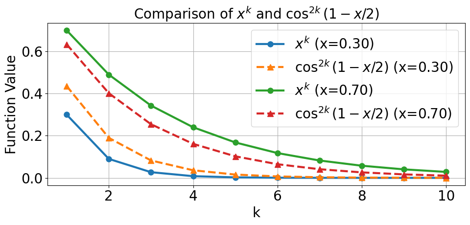
(a) $\cos^{2k}(x/2)$ vs $x^{k}$.

(b) $\cos(x)$ in $[-\pi/2,\pi/2]$.

Figure 1: Cosine function and its power. For maximization and minimization problems, the phases should be scaled based on $\cos(x)$ output. In this paper, we have used $[0,\pi/2]$ to find the minimum positive eigenvalue of $\mathcal{H}$.

Convergence: After each iteration of the algorithm, the natural normalization process scales the matrix eigenvalues. This can be seen more clearly if we write the matrix in its eigenbasis:

$$\frac{\left(I+\mathcal{U}\right)\left|\psi_{0}\right\rangle}{{\|(I+\mathcal{U})\left|\psi_{0}\right\rangle\|}}=\sum_{j}\frac{1+e^{i\lambda_{j}}}{\eta}\left|j\right\rangle\left\langle j\right|\left|\psi_{0}\right\rangle=\sum_{j}\alpha_{j}\frac{1+e^{i\lambda_{j}}}{\eta}\left(1+e^{i\lambda_{j}}\right)\left|j\right\rangle.$$ (9)

Here, $\alpha_{j}$ represents the overlap $\left\langle j|\psi_{0}\right\rangle$ and $\eta$ is a positive value representing the norm in the denominator. Since $\eta$ can be at most $|1+e^{i\lambda_{d}}|$, with $\lambda_{s}$ denoting the second-smallest eigenvalue of the Hamiltonian $\mathcal{H}$, the main contribution of the error comes from the eigenvector $\left|s\right\rangle$. Therefore, the convergence rate can be estimated by taking the magnitude of its coefficient, which simply gives the following ratio:

$$R=\frac{\cos(\lambda_{s}/2)}{\cos(\lambda_{d}/2)}.$$ (10)

After $k$ iterations, the overlap of the collapsed state with the target eigenstate $\left|d\right\rangle$ becomes proportional to the $k$th power of this ratio, $R^{k}$. Note that the power of the cosine decreases slower than the power of a similar value. However, the success probability scales with $R^{2k}$. This is shown in Fig.1, where we show how both the classical and the quantum versions require similar asymptotic numbers of iterations. This demonstrates how probabilities associated with smaller eigenvalues vanish rapidly as $k$ increases.

Furthermore, on quantum computers, this ratio does not have to be zero. It is enough to have the dominant eigenvector $\left|d\right\rangle$ in the superposition with a probability on the order of $1/n$. This way, the dominant eigenvector $\left|d\right\rangle$ can be obtained even in cases when $\mathcal{H}$ has degenerate minimum energies. To achieve a success probability $P\geq 1-\epsilon$, where $\epsilon$ represents the confidence, $R^{2k}\leq\epsilon$. Therefore, by taking the logarithm of both sides, the required number of iterations can be bounded as:

$$k\geq\frac{\ln(\epsilon)}{2\ln(R)}=\frac{\ln(1/\epsilon)}{\ln(1/R^{2})}.$$ (11)

This can be directly related to the eigengap $\gamma=\lambda_{s}-\lambda_{d}$: Since the eigenvalues are assumed to be in $[0,\pi/2]$, the ratio $R$ can be simply written as $R=\cos(\gamma/2+\lambda_{d}/2)/\cos(\lambda_{d}/2)$. For a small $\gamma$ value, this implies $R\approx 1$ and the iteration converges to the superposition of $\left|s\right\rangle$ and $\left|d\right\rangle$ and other closer eigenstates.

As mentioned before, this is fundamentally different from classical power iteration. Since on quantum computers the superposition disappears after the measurement, if we measure the quantum state at that point, we would still be able to get the dominant eigenstate if its probability in the superposition is sufficiently large. This is determined by the number of eigenstates that are close to the dominant eigenvector.

A different matter is the complexity of a single iteration: Both classical and quantum methods exhibit $\mathcal{O}(1/\gamma)$ scaling when they are applied to the unitaries. However, when we have an efficient circuit $\mathcal{U}$, i.e., a circuit with $poly(n)$ number of gates, the quantum power iteration avoids explicit matrix processing to find a circuit mapping for the unitary. Therefore, in those cases, one iteration of the algorithm only requires $O(poly(n))$ operations.

When the value of $\gamma$ is on the order of $2^{-n}$, then the required number of iterations for convergence obviously becomes exponential in the number of qubits, $O(2^{n})$. Even if $\gamma$ is not exponentially small but is on the order of $1/poly(n)$, problems with such small eigengaps may still require many iterations for convergence, which is a challenging task for current computing devices. This can be reduced if prior knowledge related to the eigenstate is available. Another approach is turning the original algorithm into a variational circuit as done in Ref.[16], which is outlined in the next section.

2 Variational Quantum Power Method (VQPM) [16]

In this section, while outlining the key points of VQPM, we will emphasize some numerical paradigms that can be encountered while using VQPM as an optimization tool to solve QUBO problems. In the next section, we will further investigate problems we have encountered in optimization results and propose some remedies for those problems.

Note that in Appendix A we give the pseudocode for the whole VQPM simulation code used in this paper and provide parameter summary in Table 1.

2.1 Parameterizing Initializing Gates

In VQPM, to reduce the number of iterations in the standard power iteration, the algorithm is converted into a variational circuit by adding rotational-$Y$ gates to the qubits representing eigenstates. This allows the state to be reinitialized by feeding the measurement outcomes (the approximate tomography) of the previous iterations. The algorithm at the $k$ iteration can simply be represented by the following circuit:

$$\Qcircuit@C=1em@R=0.5em{\lstick{\left|0\right\rangle}&\gate{H}&\qw&\ctrl{1}&\gate{H}&\meter&\qw&\rstick{\left|0\right\rangle}\\ \lstick{\left|0\right\rangle}&\gate{R_{y}(\theta_{0}^{(k-1)})}&\qw&\multigate{2}{\mathcal{U}}&\qw&\meter&\cw&\cw&\rstick{\theta_{0}^{(k)}}\\ \lstick{\left|0\right\rangle}&\gate{R_{y}(\theta_{1}^{(k-1)})}&\qw&\ghost{U}&\qw&\meter&\cw&\cw&\rstick{\theta_{1}^{(k)}}\\ \lstick{\left|0\right\rangle}&\gate{R_{y}(\theta_{2}^{(k-1)})}&\qw&\ghost{U}&\qw&\meter&\cw&\cw&\rstick{\theta_{2}^{(k)}}\\ }$$

For QUBO problems, we simply express $\left|\psi_{0}\right\rangle$ in the eigenbasis $\{\left|j\right\rangle\}$ and start with the vector:

$$\left|\psi_{0}\right\rangle=\sum_{j}\alpha_{j}\left|j\right\rangle,\quad\alpha_{j}=\frac{1}{\sqrt{2^{n}}}.$$ (12)

Therefore, for the initial state, the rotation-$y$ gates are considered as the Hadamard gates. Since any of the eigenvectors $\left|j\right\rangle$ is an unentangled tensor product state, this circuit is able to represent all the eigenstates by giving the right parameters to the single gates. However, the circuit at the end generates a final state which is the superposition of many eigenstates.

This circuit provides a way to feed the previous output state to the next iteration by individual qubit measurements. Thus, it does not necessitate a full quantum state tomography and can be considered as a very efficient circuit.

2.1.1 Measurement and Information Loss

While measuring the state, the probabilities of the eigenstates are determined by the magnitude of the overlap $|\alpha_{j}^{(k)}|$ for the $j$th state. When we have a bias in the state $\left|\psi_{k-1}\right\rangle$ toward some eigenstates, since the changes in $|\alpha_{j}^{(k)}|$ are proportional to the eigenvalue ratio $R$ for the $j$th eigenvalue and its eigengap, it is possible that the bias in the previous state cannot be reversed in one iteration.

In other words, when we measure the qubit, in the early states the probability of the qubits may be directed toward the eigenstate group for which the dominant eigenvalue does not belong. Therefore, when the eigengap is small, if we measure the probabilities in high precision especially in the early iterations, surprisingly it may cause us to lose some part of the solution space, where the dominant eigenvalue belongs, for the rest of the iterations. This is depicted for a random instance of QUBO in Fig.2, where, after some iterations, the further iterations take the algorithm further away from the dominant eigenstate to another eigenstate whose energy value is very close to the dominant eigenvalue. Therefore, in the early iterations it may be advisable to use very low precision for the qubit measurements: note that in that case, the convergence may become very slow or stagnate at the same value.

Fig.3(a) shows, for 100 random QUBO trials of $n=15$ parameters, how the success probability of the target (optimum) state increases and whether in these trials the optimization converges to different values. To indicate whether it has converged to a different value, we count the number of parameter values (0 or 1) that are different from the optimum solution. Similarly, Fig.3(b) shows the mean success probability and the mean number of bit difference values for $n=1\dots 18$ using 500 iterations and 100 trials for each $n$ value. As can be seen from the lower right side of the figure, the mean success probability approaches the exponential line, which indicates that the convergence is still bounded by the eigengap. This can be remedied by increasing the number of iterations; however, in that case, the required number of iterations would increase with the eigengap.

Therefore, for the above complexity dilemma, to reduce the required number of iterations and to increase the success probability at the same time, a locking mechanism is introduced to the algorithm: In each iteration, we check to see whether the probability difference of measuring 0 or 1 for a qubit is above a certain threshold. If yes (say, if the probability for 0 is much higher), then we lock that qubit to 0 (or 1 based on the difference). Below, this is described and analyzed in further detail.

Figure 2: Incorrect convergence may be caused by bias in the probabilities of the qubits from the early measurement results. The optimization converges to a close value, but it is another eigenstate.

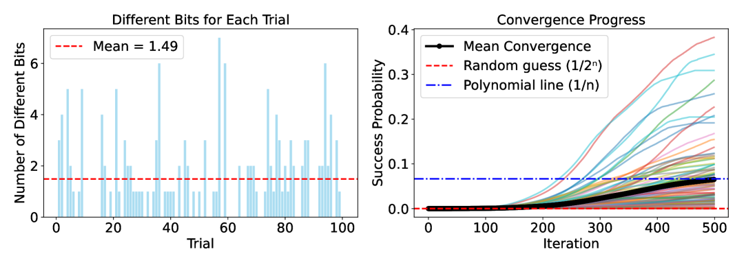
(a) Convergence for 100 random trials of QUBO problems for $n=15$ qubits. The convergence is slow, especially when the eigengap is small. Incorrect bit flips due to the early measurement results cause a bias in the probabilities of the qubits, which gives higher probabilities for the other eigenvectors in the state.

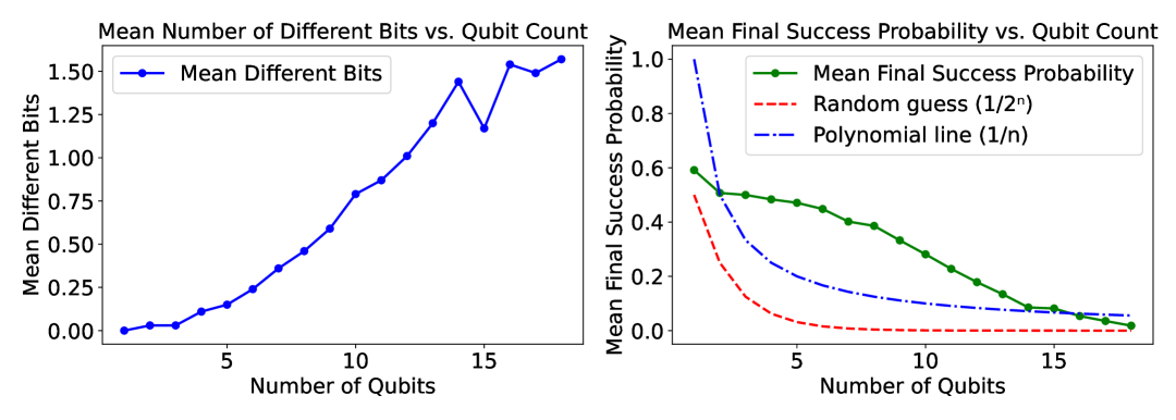
(b) Mean convergence for 100 random trials of QUBO problems for $n=1\dots 18$ qubits. The maximum number of iterations is set to 500. The mean final success probability decreases exponentially, which is related to the eigengap generally determined by the dimension in these random trials.

Figure 3: VQPM without locking the qubits. The algorithm converges to a suboptimal value if the measurements on the qubits introduce a bias in the early iterations.

2.2 Locking Qubits

As explained earlier, in addition to parameterizing the circuit, the second setting for VQPM is: If any qubit value can be determined in the earlier iterations, then these qubit states are locked to that determined value (set to 0 or 1 for the rest of the iterations). That means if the probability difference between 0 and 1 for any qubit is larger than an optimization parameter $p_{diff}$, then the values of these qubits are locked to $\{0,1\}$ depending on the outcome. This can be considered as jumps in the iterations. An example of such jumps is depicted in Fig.4(a) for $n=15$ qubits. As can be seen from the figure, the algorithm converges to the solution in just 15 iterations. Note that this is not a marginal case. Fig.5 shows the same running test (the random seed is set to 42 while generating QUBO problem groups) as used for the case without locking. However, in this case, we only use a maximum of 30 iterations for $n=1\dots 18$ and obtain much better results.

In the simulation, we set $p_{diff}=0.01$ and measurement precision to 3 decimal places (the probabilities are rounded to 3 decimals, e.g., 0.512 and 0.488). These values were the best values we have observed for $n\leq 20$ parameters. We have not run the algorithm for larger $n>20$ simulations. However, from our observations, it is likely to require more iterations instead of an adjustment to these parameters.

From the figures, it can also be seen that it is possible to lock some qubits to the wrong values, which would cause the algorithm to converge to a wrong solution. In the next section, we analyze this incorrect locking and suggest some solutions to remedy this problem.

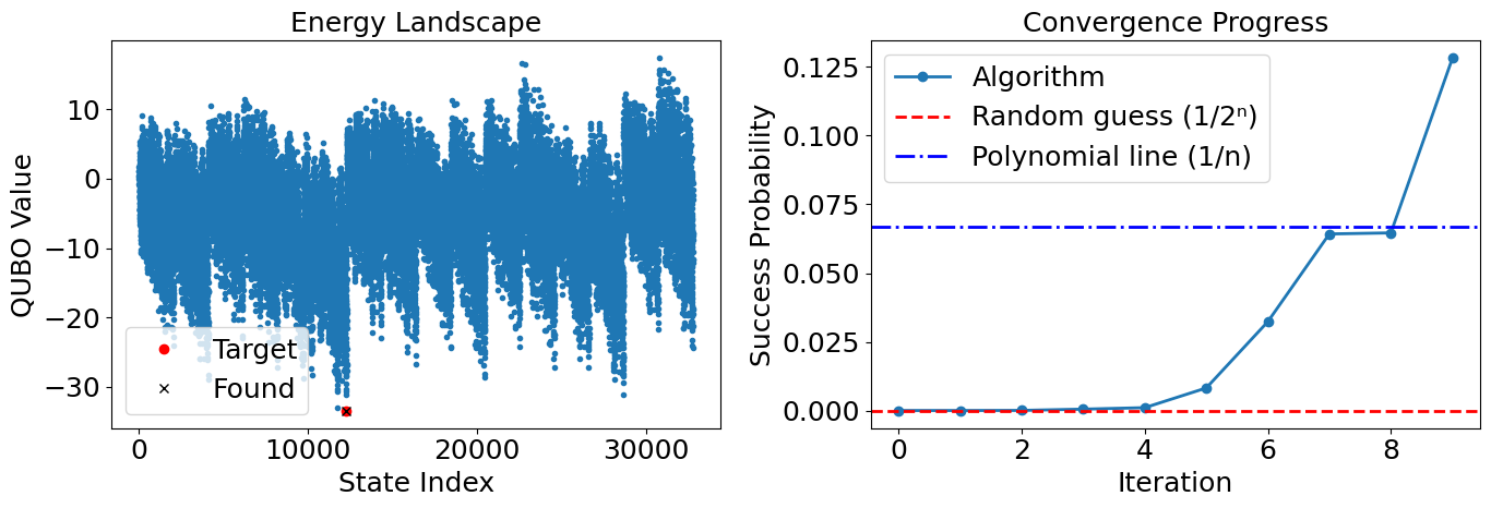
(a) Jumps in the iteration by locking qubits to the values early in the iterations: The optimization converges to the correct value in only a few iterations.

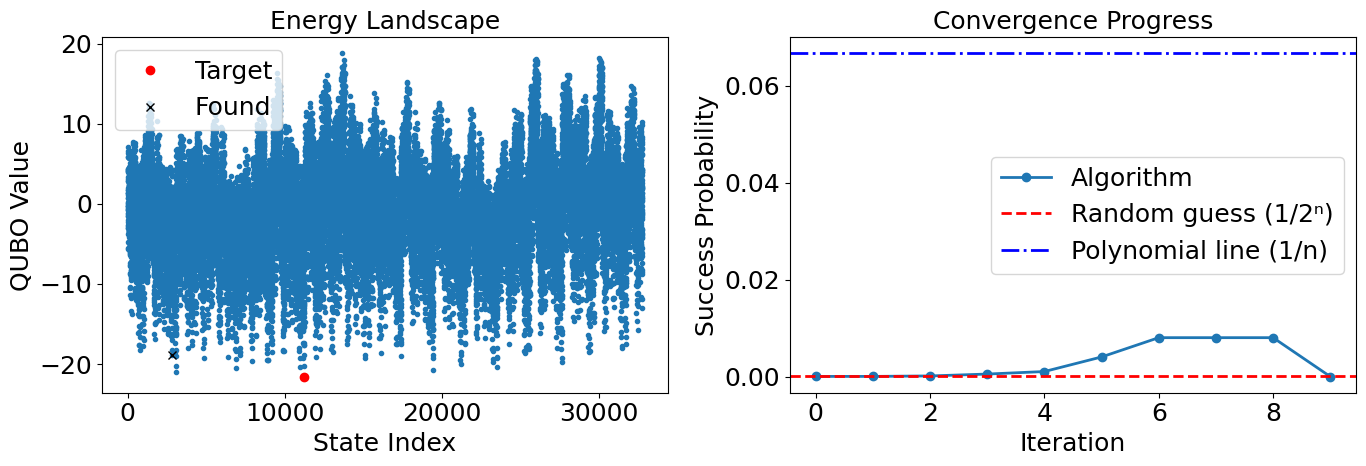
(b) Jumps in the iteration by locking qubits to the values early in the iterations: The optimization converges to a suboptimal value because of an early incorrect locking.

Figure 4: The correct and incorrect locking in VQPM for two random 15-parameter QUBO trials.

3 Incorrect Locking and Minimizing its Impact

3.1 Incorrect Locking

As mentioned earlier, a downside of this approach is the early locking of some qubit values: For a qubit $q$ with the probabilities $P_{0}$ for $q=0$ and $P_{1}$ for $q=1$, $P_{diff}=|P_{0}-P_{1}|$. By letting $S_{0}$ and $S_{1}$ denote the eigenstates where $q=0$ and $q=1$, respectively, the probabilities after $k$ iterations can be defined as:

$$P_{0}^{(k)}=\frac{\sum_{j\in S_{0}}|1+e^{i\lambda_{j}}|^{2k}}{\sum_{j}|1+e^{i\lambda_{j}}|^{2k}},\quad P_{1}^{(k)}=\frac{\sum_{j\in S_{1}}|1+e^{i\lambda_{j}}|^{2k}}{\sum_{j}|1+e^{i\lambda_{j}}|^{2k}}.$$ (13)

Here, the cardinalities of the sets are equal, $|S_{0}|=|S_{1}|=2^{n-1}$, and the dominant eigenvalue can be a member of the same set as the group of eigenvalues with the lowest magnitudes (this can be considered a marginal case for the qubit).

Therefore, a“mistake” (e.g., incorrectly locking $q=1$ while $d\in S_{0}$) can occur if $P_{diff}^{(k)}>p_{diff}$. This leads the algorithm to automatically eliminate the solution from the search space. This is shown in Fig.4(b), where the third locking of a qubit value causes the removal of the optimum eigenvalue from the remaining search space, and the algorithm converges to a different eigenvalue. This incorrect locking can occur in any iteration; however, while in the early iterations it can occur arbitrarily, in the later iterations it is more likely to occur between the dominant eigenvalue and values that are closer to it. This can be prevented to some extent by setting $p_{diff}$ high for early iterations and lowering it toward the later iterations. Note that a lower value of $p_{diff}$ requires higher precision in the measurements and lower error rates in the circuit.

Here note that the energy landscape generated by the coefficients in $Q$ is squeezed into the eigenphases in $[0,\pi/2]$. This may cause some values to be lost because of numerical rounding and cut-off errors if the eigengap is too small. In addition, in some cases the energies are too close to each other and may be degenerate, having multiple optimal values. In our simulations, we do not check for this situation. Therefore, some of the convergence mistakes may be justified.

Also note that in our experiments we always use the equal superposition state as an initial state. To minimize the incorrect early locking effect, one intuitive method is to start the algorithm with a different initial vector. However, this would require more parameterized gates and would change the algorithm into a variational quantum eigensolver. Instead of this, one can try setting the critical bits to different values and run the algorithm with this setting. However, for larger problem instances, it is hard to find which qubits are critical. Below, we will describe dynamic $p_{diff}$ settings for these cases, where a different value is used for every iteration or for each qubit based on its influence.

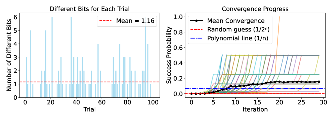
(a) 100 random QUBO trials for $n=15$ with fixed $p_{diff}=0.01$ and precision is 3 (the probabilities are rounded to three decimals by using the NumPy round function).

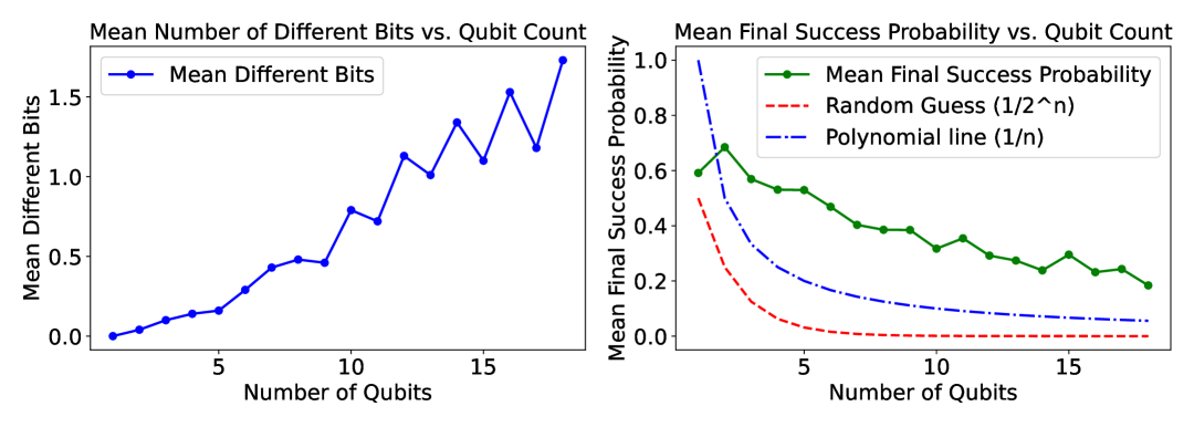
(b) The convergence for the mean values of 100 random trials of QUBO problems for $n=1\dots 18$ qubits. The maximum number of iterations is set to 30.

Figure 5: VQPM with locking of the qubits by using fixed $p_{diff}=0.01$ and a measurement precision of 3 (the probabilities are rounded to three decimals by using the NumPy round function). The algorithm converges to a suboptimal value if there is an incorrect locking or if the suboptimal values have higher probabilities.

3.2 Dynamic $p_{diff}$

Below we describe different approaches that can be used based on the problem specifics. Note that these approaches do not necessarily improve the results on random instances; however, they may be useful in certain cases.

3.2.1 The Bit Significance Based Approach

One idea would be to scale $p_{diff}$ based on the significance of the bits in the order of their values, i.e., applying early locking only to the least significant bits. However, this does not make the error in the end any better because by locking even the least significant bit we may be disregarding the dominant eigenvector or many other close suboptimal eigenstates in the solution space. Thus, although the probabilities would be biased toward the region where the dominant eigenvalues are located, we did not see any benefit in using this approach. This approach may only be useful in certain applications where one has some knowledge of the solution space distribution.

3.2.2 Scaling Based Approach

Another approach would be to start with an initially higher value, i.e., $p_{diff}^{(0)}\gg 0$, in order to prevent early elimination of the dominant eigenvalue because of incorrect locking. A simple method for dynamic $p_{diff}$ is to scale it proportionally to the iteration $k$. For instance, one can use the following:

$$p_{diff}^{(k)}=\frac{p_{diff}^{(k-1)}}{f(k)},$$ (14)

where $f(k)$ is a function of $k$, e.g., $2^{k}$. In this case, the starting point becomes important. In the classical simulations, as stated, the best pair of values for $(p_{diff},\text{precision})$ that we have observed is $(0.01,3)$. Lowering these values means increasing the number of measurements. Therefore, one can only start with a high $p_{diff}$ and scale it by the iterations to a minimum of approximately 0.01. A too-high $p_{diff}$ would convert the VQPM into the version with no qubit locking. Therefore, the scaling would be similar to the results depicted in Fig.3.

3.2.3 Hoeffding’s Inequality Based Approach

(a) 100 random QUBO trials for $n=15$ with dynamic $p_{diff}\in[0.005,0.15]$ determined from Hoeffding’s inequality given in Eq.19 and precision is 3 (the probabilities are rounded to three decimals by using the NumPy round function).

(b) The convergence for the mean values of 100 random trials of QUBO problems for $n=1\dots 18$ qubits. The maximum number of iterations is set to 30.

Figure 6: VQPM with a dynamic $p_{diff}\in[0.005,0.15]$ determined from Hoeffding’s inequality by using $\delta_{total}=0.5$, $M=100$, $10nM=1000n$, the maximum iteration number is 30, and precision is 3 (the probabilities are rounded to three decimals by using the NumPy round function).

A more rigorous approach for determining the value of $p_{diff}$ can be achieved through probability theory. This can be accomplished by using Hoeffding’s inequality, or similar methods, along with the number of measurements (the inverse of the precision) and the expected error rate.

Hoeffding’s inequality [19] is a foundational tool in probability theory and statistical learning theory, which is used to provide an upper bound on the probability that the sample average deviates from the expected value $\mathbb{E}[X]$ by a certain amount $\epsilon$. For a set of independent bounded random variables $X_{1},\dots,X_{M}\in[a,b]$, the inequality is defined as:

$$P\left(\left|\frac{1}{M}\sum_{i=1}^{M}X_{i}-\mathbb{E}[X]\right|\geq\epsilon\right)\leq 2\exp\left(-\frac{2M\epsilon^{2}}{(b-a)^{2}}\right).$$ (15)

This inequality can be repurposed in the context of VQPM to bound the error ($p_{diff}$) in estimating qubit probabilities from a finite number of quantum measurements (i.e., the number of repetitions, or shots). When estimating the probability $P_{0}$ of a qubit being in state $|0\rangle$, $M$ shots yield an empirical estimate $\hat{P}_{0}$. Hoeffding’s inequality guarantees that this estimate is below a certain threshold with the probability defined as [20]:

$$P\left(|\hat{P}_{0}-P_{0}|\geq\epsilon\right)\leq 2e^{-2M\epsilon^{2}}.$$ (16)

Rearranging for $\epsilon$, the maximum error $\epsilon$ with confidence $1-\delta$ is:

$$\epsilon=\sqrt{\frac{\ln(2/\delta)}{2M}}.$$ (17)

Here, $\delta$ represents the failure rate, and it can be distributed across the iterations by using a union bound:

$$\delta_{k}=\frac{\delta_{\text{total}}}{\text{remaining iterations}}.$$ (18)

The deviation threshold $\epsilon$ in our case becomes the adaptive $p_{diff}$ threshold—the minimum probability difference required to confidently lock the state of a qubit. However, the standard equation for $\epsilon$ gives values that are too large. In order to keep the value in the range $\approx[0.015,0.005]$ for $n\leq 20$, we set the values $M=100$ and $\delta_{total}=0.5$, and incorporate the number of parameters (qubits) in the equation as $10n$:

$$\epsilon=\sqrt{\frac{\ln(2/\delta)}{2\times(10nM)}}.$$ (19)

Since this value gives a higher $p_{diff}$ for smaller $n$ and a lower $p_{diff}$ for larger $n$, it incorporates the growth of the solution space.

Fig.6 shows the running of the algorithm with a maximum of 30 iterations for the same problem set. From the figures, it can be seen that overall performance is slightly worse than when using fixed $p_{diff}$ for locking. However, in some instances where the fixed version is unable to find the solution, the dynamic probability converges to the optimum or a better solution. This indicates that in some cases it may be more appropriate to use a dynamic difference.

3.3 Influence Scores Based Approach

Another dynamic approach is to use different $p_{diff}$ values based not on their significance order in the bit value, but on how their change may affect the energy eigenvalue. This can be computed through the coefficients given by $Q$. We define the influence for a parameter (a qubit) $i$ as:

$$\text{Influence}(i)=\frac{\sum_{j}|Q_{ij}|}{\|Q\|_{\infty}}.$$ (20)

Here, the infinity norm is defined as:

$$\|Q\|_{\infty}=\max_{i}\sum_{j}|Q_{ij}|,$$ (21)

which represents the maximum influence. Note that the influence scores are used in molecular similarity and network alignment problems, which are solved by obtaining the dominant eigenvector [21].

Fig.7 shows the results where the individual $p_{diff}$ for qubits are scaled based on their influences. This gives slightly better results than the dynamic $p_{diff}$ determined from Hoeffding’s inequality alone.

(a) 100 random QUBO trials for $n=15$ with dynamic $p_{diff}\in[0.005,0.15]$ determined from Hoeffding’s inequality and influence scores of each qubit, with precision 3 (the probabilities are rounded to three decimals by using the NumPy round function).

(b) The convergence for the mean values of 100 random trials of QUBO problems for $n=1\dots 18$ qubits. The maximum number of iterations is set to 30.

Figure 7: VQPM based on influence scores and with a dynamic $p_{diff}\in[0.005,0.15]$ determined from Hoeffding’s inequality using $\delta_{total}=0.5$, $M=100$, $10nM=1000n$; the maximum iteration number is 30. The found $p_{diff}$ is scaled for each qubit based on their influences. The precision is again 3 (the probabilities are rounded to three decimals by using the NumPy round function).

4 The Role of the Control Qubit in Optimization

The controlled gate acts in the same way as in the phase estimation algorithm. Its probability of $\left|0\right\rangle$ converges to an eigenvalue ($1+e^{i\lambda_{j}}$) associated with the converged $j$th eigenstate—in our case, if the eigenstate is the one with the largest eigenvalue in magnitude of $I+U$.

This qubit can be used to prevent any sudden jumps due to incorrect locking. Therefore, it can also prevent the optimization from converging to an eigenvalue that is too far away from the optimum. This is particularly significant in cases where there are two groups of eigenvalues, one with small and the other with large magnitudes. This shows that the algorithm is almost guaranteed to converge to the larger eigenvalues. Therefore, we have a kind of lower threshold mechanism.

However, any further use of this qubit in the optimization may require extreme precision and increase the complexity. For instance, using the qubit as a means to fully control the locking mechanism—if the optimization improves the eigenvalue (that is, if the probability of $\left|0\right\rangle$ increases), then we lock; otherwise, we use the measured probabilities for the qubit.

In our simulations, we fixed the precision to three decimal places. In this scenario, we did not observe any improvement or change in the optimization. This does not mean that this approach cannot be further employed; it just means that in the simulations, the probability of the qubits is mainly determined by the larger eigenvalues. Therefore, the optimization generally does not make big jumps toward the smaller eigenvalues. However, for larger cases, one may integrate this into a classical optimization algorithm along with the parameters of the rotation gates.

5 A Simple Numerical Comparison to QAOA

(a) $n=4$

.

(b) $n=6$

Figure 8: Comparison for $n=6$ on 100 random trials. Final probabilities of the target state for the same problem sets. For VQPM, we have used fixed $p_{diff}=0.01$ and precision 3 with 30 maximum iterations. For QAOA, we have used a standard circuit with $p=8$, the number of layers.

In Fig.8 we compare the performance of the VQPM with QAOA on the same randomly generated trial data set for $n=4$ and $n=6$. It is known that the performance of QAOA is highly dependent on the optimizer, circuit depth, and the number of iterations. When these are handled correctly, the algorithm is able to solve many difficult problems. While its convergence also depends on the eigengap, it guarantees a solution. However, the overall mean values are in general better for VQPM in our experiments.

6 Conclusion and Future Directions

The QUBO formulation has a wide spread of use in science, where we model many real-world problems as an eigenvalue optimization. For instance, the graph-cut problem, with its standard QUBO formulation, can be seen in the solution of many real-world problems such as optimizing the labeling problem [22]. In these problems, a graph-cut is defined as a problem of minimizing a quadratic energy function [6].

Since the basic graph-cut tries to distinguish vertices into two disjoint sets, VQPM can be a perfect model for it because it also divides eigenvalues into groups based on the qubit states in their eigenstates. Therefore, thanks to the explicit amplitude amplification via $(I+U)^{k}$ and its mechanism to reduce the solution space exponentially by locking qubits to their values, we believe it warrants separate analysis and can be employed in real-world problems.

In this paper, we have investigated many details of VQPM and provided alternatives for choosing the locking mechanism of the algorithm. We believe it can serve as a guide for further applications in different fields.

7 Data availability

The simulation code used to generate all figures presented in this paper is publicly available on: https://github.com/adaskin/vqpm The pseudocode for VQPM is given in Appendix A and the parameters are given in Table 1.

8 Funding

This project is not funded by any funding agency.

9 Acknowledgment

When writing simulation code, we acknowledge that we have benefited suggestions from various AI tools mainly: Microsoft Copilot [23] and DeepSeek-R1/V3 [24] . And the paper and the equations have been proofread, without changing the structures of the paragraphs and sentences, by using Microsoft Copilot [23].

Appendix A Algorithmic Flowchart for VQPM

1:Initialize:

2: - Random QUBO matrix $Q$

3: - Adjust phase: $Q\to Q_{\text{scaled}}$

4: - Construct unitary $U$ from $Q_{\text{scaled}}$

5: - Initialize $\psi_{0}=\frac{1}{\sqrt{2^{n}}}\sum_{j}\left|j\right\rangle$

6:for $k=1$ to max_iter do

7:  Apply variational circuit:

8:   - $\psi_{1}=U\cdot\psi_{0}$

9:   - $\psi_{\text{final}}=\frac{\psi_{0}+\psi_{1}}{\sqrt{2}}\quad(\text{simulate }I+U)$

10:  Calculate probabilities:

11:   - $p_{\text{min}}=\max|\psi_{\text{final}}|^{2}$

12:  Convergence check:

13:  if $p_{\text{min}}\geq 0.5$ then

14:    - Break (success)

15:  end if

16:  if target state is given then

17:   if converged to target state then

18:      - Break (success)

19:   end if

20:   if probability of target state has become 0 then

21:      - Break (failure)

22:   end if

23:  end if

24:  Dynamic $p_{diff}$ adjustment (If chosen):

25:   - $p_{diff}^{(k)}=\sqrt{\frac{\ln(2/\delta_{i})}{2\cdot 10nM}}\quad(\delta_{i}=\delta_{\text{total}}/\text{max\_iter})$

26:   - scale for each qubit by influence scores (if chosen)

27:  Prepare new state:

28:  for each qubit $q\in\{1,...,n\}$ do

29:    - Measure $P_{0}^{(q)},P_{1}^{(q)}$

30:   if $|P_{0}^{(q)}-P_{1}^{(q)}|\geq p_{diff}^{(k)}$ then

31:      - Collapse qubit $q$ to $\arg\max(P_{0}^{(q)},P_{1}^{(q)})$

32:   else

33:      - Keep superposition with the probabilities $P_{0}^{(q)},P_{1}^{(q)}$

34:   end if

35:  end for

36:  Update $\psi_{0}$ for next iteration

37:end for

38:Output:

39: - Found state $s_{\text{final}}=\text{argmax}(|\psi_{\text{final}}|^{2})$

40: - Success probability of the found $p_{\text{min}}$

41: - Probability of the target (if known $|\psi_{\text{final}(\text{target state})}|^{2})$

Table 1: Summary of Key Parameters in the Code and Their Ranges

Parameter	Purpose	Typical Range	Impact
$n$	Number of qubits	1–20	Scales state space as $2^{n}$. Larger $n$ increases complexity.
max_iter	Maximum iterations	10–50	Higher values may improve convergence if $p_{diff}$ is small enough.
$p_{diff}$	Collapse threshold	0.01 or (dynamic [0.005, 0.015])	Balances superposition preservation (low) vs. decision speed (high).
precision	Rounding precision for probabilities	3 (best choice) or 3–7 decimal places
shots_per_iter ($M$)	Measurements per iteration	100–1000	Reduces noise via $\propto 1/\sqrt{M}$. Higher $M$ increases cost.
delta_total	Total failure probability	0.01–0.1	Lower $\delta$ increases reliability but requires more shots.
qubit_weights	Qubit influence weights	[0, 1] (normalized)	Prioritizes high-impact qubits via $p_{diff}$-scaling.

References

- [1] Fernando GS L Brandao, Richard Kueng, and Daniel Stilck França. Faster quantum and classical sdp approximations for quadratic binary optimization. Quantum, 6:625, 2022.
- [2] Fred Glover, Gary Kochenberger, Rick Hennig, and Yu Du. Quantum bridge analytics i: a tutorial on formulating and using qubo models. Annals of Operations Research, 314(1):141–183, 2022.
- [3] Iain Dunning, Swati Gupta, and John Silberholz. What works best when? a systematic evaluation of heuristics for max-cut and qubo. INFORMS Journal on Computing, 30(3):608–624, 2018.
- [4] Martin Anthony, Endre Boros, Yves Crama, and Aritanan Gruber. Quadratic reformulations of nonlinear binary optimization problems. Mathematical Programming, 162:115–144, 2017.
- [5] Svatopluk Poljak and Franz Rendl. Solving the max-cut problem using eigenvalues. Discrete Applied Mathematics, 62(1-3):249–278, 1995.
- [6] Vladimir Kolmogorov and Ramin Zabin. What energy functions can be minimized via graph cuts? IEEE transactions on pattern analysis and machine intelligence, 26(2):147–159, 2004.
- [7] Rimmi Anand, Divya Aggarwal, and Vijay Kumar. A comparative analysis of optimization solvers. Journal of Statistics and Management Systems, 20(4):623–635, 2017.
- [8] Tad Hogg and Dmitriy Portnov. Quantum optimization. Information Sciences, 128(3-4):181–197, 2000.
- [9] Edward Farhi, Jeffrey Goldstone, Sam Gutmann, and Michael Sipser. Quantum computation by adiabatic evolution. arXiv preprint quant-ph/0001106, 2000.
- [10] Wim Van Dam, Michele Mosca, and Umesh Vazirani. How powerful is adiabatic quantum computation? In Proceedings 42nd IEEE symposium on foundations of computer science, pages 279–287. IEEE, 2001.
- [11] Dorit Aharonov, Wim Van Dam, Julia Kempe, Zeph Landau, Seth Lloyd, and Oded Regev. Adiabatic quantum computation is equivalent to standard quantum computation. SIAM review, 50(4):755–787, 2008.
- [12] Aleta Berk Finnila, Maria A Gomez, C Sebenik, Catherine Stenson, and Jimmie D Doll. Quantum annealing: A new method for minimizing multidimensional functions. Chemical physics letters, 219(5-6):343–348, 1994.
- [13] A Yu Kitaev. Quantum measurements and the abelian stabilizer problem. arXiv preprint quant-ph/9511026, 1995.
- [14] Edward Farhi, Jeffrey Goldstone, and Sam Gutmann. A quantum approximate optimization algorithm. arXiv preprint arXiv:1411.4028, 2014.
- [15] Filipe FC Silva, Pedro MS Carvalho, Luís AFM Ferreira, and Yasser Omar. A qubo formulation for minimum loss network reconfiguration. IEEE Transactions on Power Systems, 38(5):4559–4571, 2022.
- [16] Ammar Daskin. Combinatorial optimization through variational quantum power method. Quantum Information Processing, 20(10):336, 2021.
- [17] Ammar Daskin. The quantum version of the shifted power method and its application in quadratic binary optimization. arXiv preprint arXiv:1809.01378, 2018.
- [18] Gene H. Golub and Charles F. van Loan. Matrix Computations. JHU Press, fourth edition, 2013.
- [19] Wassily Hoeffding. Probability inequalities for sums of bounded random variables. The collected works of Wassily Hoeffding, pages 409–426, 1994.
- [20] J. M. Phillips. Chernoff-hoeffding inequality and applications. ArXiv, abs/1209.6396, 2012.
- [21] Anmer Daskin, Ananth Grama, and Sabre Kais. Multiple network alignment on quantum computers. Quantum information processing, 13(12):2653–2666, 2014.
- [22] Nikos Komodakis and Georgios Tziritas. Approximate labeling via graph cuts based on linear programming. IEEE transactions on pattern analysis and machine intelligence, 29(8):1436–1453, 2007.
- [23] Microsoft Copilot. Private communication, May 2025. Personal communication.
- [24] DeepSeek-R1/V3 Chat. Private ai-assisted communication, May 2025. Conversation with Microsoft Copilot/DeepSeek AI system.