SplInterp: Improving our Understanding and Training of Sparse Autoencoders

Abstract

Sparse autoencoders (SAEs) have received considerable recent attention as tools for mechanistic interpretability, showing success at extracting interpretable features even from very large LLMs. However, this research has been largely empirical, and there have been recent doubts about the true utility of SAEs. In this work, we seek to enhance the theoretical understanding of SAEs, using the spline theory of deep learning. By situating SAEs in this framework: we discover that SAEs generalise “$k$-means autoencoders” to be piecewise affine, but sacrifice accuracy for interpretability vs. the optimal “$k$-means-esque plus local principal component analysis (PCA)” piecewise affine autoencoder. We characterise the underlying geometry of (TopK) SAEs using power diagrams. And we develop a novel proximal alternating method SGD (PAM-SGD) algorithm for training SAEs, with both solid theoretical foundations and promising empirical results in MNIST and LLM experiments, particularly in sample efficiency and (in the LLM setting) improved sparsity of codes. All code is available at: https://github.com/splInterp2025/splInterp

1 Introduction

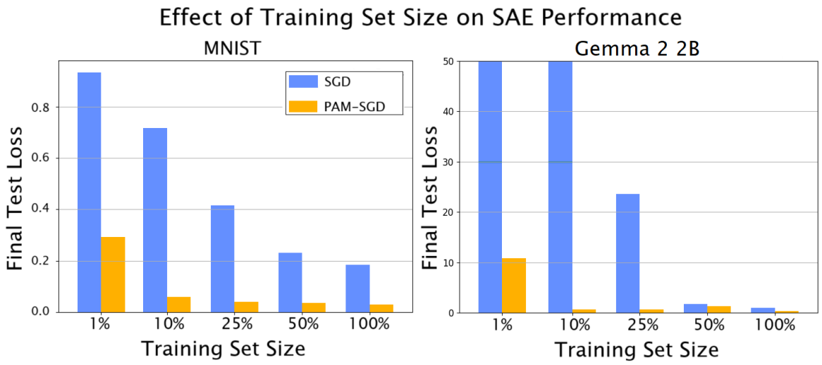
Figure 1: Key ideas in this work. Left: Sparse autoencoders (SAEs) vs. regular autoencoders; in an SAE, the code $z$ can have very high dimension, but most entries are zero (greyed out). Right: The superior sample efficiency (on MNIST and Gemma-2-2B) of our novel proximal alternating method SGD (PAM-SGD) algorithm.

One of the fundamental challenges in modern AI is the interpretability of machine learning systems: how can we look inside these increasingly more complicated (and capable) “black boxes”? The better we understand what makes these systems tick, the better we can diagnose problems with them, direct their behaviour, and ultimately build more effective, reliable, and fair systems. Indeed, for some tasks interpretability may be a legal requirement, for example Article 86 of the European Union’s AI Act describes a “right to explanation” for persons affected by the decisions of certain types of AI system.

A mechanistic interpretability technique that has seen considerable recent attention is to use sparse autoencoders (SAEs), see e.g. Bricken et al. (2023); Huben et al. (2024); Gao et al. (2025). A major obstacle in interpreting a neural network is that neurons seem to be polysemantic, responding to mixtures of seemingly unrelated features Olah et al. (2017). One hypothesis is that this is caused by superposition, a phenomenon in which a neural network represents features via (linear) combinations of neurons, to pack in more features. In Elhage et al. (2022), superposition was shown to arise in a toy model in response to sparsity of the underlying features. The key idea of using SAEs was that these might be able to disentangle this superposition and extract monosemantic features.

Initial work found some success, e.g. Templeton et al. (2024) used SAEs to extract millions of features from Claude 3 Sonnet, including highly interpretable ones such as a “Golden Gate Bridge” feature, which could be used to make Claude incessantly talk about the bridge. However, there have been some recent doubts about the utility of SAEs for mechanistic interpretability. In a recent post by the Google DeepMind mechanistic interpretability team Smith et al. (2025), works finding key issues with SAEs were highlighted, e.g. Leask et al. (2025), and SAEs were found to underperform linear probes at a downstream task. The team argued that whilst SAEs are not useless, they will not be a game-changer for interpretability, and speculated that the field is over-invested in them. Furthermore, in what we will dub a “dead salmon” experiment (in honour of Bennett et al. (2009)), Heap et al. (2025) found that SAEs can extract features from randomly weighted Transformers that have very similar auto-interpretability scores to features extracted from a trained network–suggesting that SAE “interpretations” may not reflect what is actually going on in a model.

This empirical uncertainty motivated us to look at SAEs through a more theoretical lens, inspired by the spline theory of deep learning Balestriero & Baraniuk (2018). Using this perspective, we:

1. Unify, situating SAEs within the spline theory framework, and showing how SAEs form a bridge between the classical ML techniques of $k$-means and principal component analysis (PCA) and contemporary deep learning. (Section˜2, proofs in Appendix˜B)

2. Interpret, characterising and visualising the spline geometry of (TopK) SAEs in terms of weighted Voronoi diagrams. (Sections˜2, A and B)

3. Innovate, developing a novel proximal alternating method SGD (PAM-SGD) algorithm for training SAEs, with both solid theoretical foundations and promising empirical results, which is inspired by the spline geometric way of thinking. In particular, we find in both MNIST and LLM experiments that PAM-SGD outperforms SGD in low-training-data settings, addressing an important concern with SAEs. (Sections˜3, C and E)

2 The spline geometry of sparse autoencoders (SAEs)

2.1 A primer on SAEs

An SAE composes an encoding, which maps an input $x\in\mathbb{R}^{n}$ to a code $z\in\mathbb{R}^{d}$ (enginereed to be sparse), with a decoding which maps $z$ to an output $\hat{x}\in\mathbb{R}^{n}$ (engineered so that $\hat{x}\approx x$). Unlike a traditional autoencoder, in an SAE one may choose the hidden dimension $d\gg n$, but the sparsity of $z$ will be engineered to be much less than $n$, see Figure˜1(left). The SAE encoding is given by

$$z:=\rho(W_{\text{enc}}x+b_{\text{enc}}),$$

where $W_{\text{enc}}\in\mathbb{R}^{d\times n}$, $b_{\text{dec}}\in\mathbb{R}^{d}$, and $\rho$ is a given activation function. Notable choices for $\rho$ include ReLU Bricken et al. (2023), JumpReLU Rajamanoharan et al. (2024) where $\tau\in\mathbb{R}$ is a parameter and

$$\rho(v)_{i}:=\begin{cases}v_{i},&\text{if }v_{i}>\tau,\\ 0,&\text{otherwise},\end{cases}$$

and TopK Makhzani & Frey (2014); Gao et al. (2025) where $K\in\mathbb{N}$ is a parameter and

$$\rho(v)_{i}:=\begin{cases}v_{i},&\text{if $v_{i}$ is among the $K$ largest entries of $v$,}\\ 0,&\text{otherwise}.\end{cases}$$

The decoding is then given by

$$\hat{x}:=W_{\text{dec}}z+b_{\text{dec}},$$

where $W_{\text{dec}}\in\mathbb{R}^{n\times d}$ and $b_{\text{dec}}\in\mathbb{R}^{n}$. The columns of $W_{\text{dec}}$ can be understood as dictionary atoms (see Olshausen & Field (1996)) which are sparsely recombined (with bias) to recover $\hat{x}$.

The full SAE is therefore given by

$$S_{\rho}(x) :=W_{\text{dec}}\rho(W_{\text{enc}}x+b_{\text{enc}})+b_{\text{dec}}.$$

Finally, following Rajamanoharan et al. (2024), given training data $\{x^{r}\}_{r=1}^{N}\in\mathbb{R}^{n}$, we will consider loss functions for training an SAE of the form:

$$\mathcal{L} =\sum_{r=1}^{N}\|S_{\rho}(x^{r})-x^{r}\|_{2}^{2}+\lambda\mathcal{L}_{\text{sparsity}}\left(\{\rho(W_{\text{enc}}x^{r}+b_{\text{enc}})\}_{r=1}^{N}\right)+\mathcal{L}_{\text{aux}},$$

where $\mathcal{L}_{\text{aux}}$ might include regularisation, e.g. weight decay. Some activations, e.g. TopK, always produce a sparse $z$, so one may set $\mathcal{L}_{\text{sparsity}}=0$. Others, e.g. ReLU, do not inherently make $z$ sparse, in which case common choices of $\mathcal{L}_{\text{sparsity}}$ include the $\ell_{1}$ norm Bricken et al. (2023), the $\ell_{0}$ norm Rajamanoharan et al. (2024), and the Kullback–Leibler divergence to a sparse distribution Ng (2011).

2.2 SAEs are piecewise affine splines

We first note a simple fact about our SAEs, also observed in Hindupur et al. (2025) (in different notation). In all three cases of ReLU, JumpReLU, and TopK, for some $S\subseteq\{1,...,d\}$ we have that

$$\rho(v)=P_{S}v,$$

where $P_{S}\in\mathbb{R}^{d\times d}$ is the projection that zeroes the entries of $v$ which are not in $S$. In the case of JumpReLU (of which ReLU is a special case) $S$ is the set of indices $i$ such that $v_{i}>\tau$, and in the case of TopK $S$ is the set of indices containing the largest $K$ entries. Therefore, let us define

$$\Omega_{S}^{\operatorname{JumpReLU}} :=\{x\in\mathbb{R}^{n}:\forall i\in S,(W_{\text{enc}}x+b_{\text{enc}})_{i}>\tau\text{ and }\forall j\notin S,(W_{\text{enc}}x+b_{\text{enc}})_{j}<\tau\},$$

$$\Omega_{S}^{\operatorname{TopK}} :=\{x\in\mathbb{R}^{n}:\forall i\in S,j\notin S,\>(W_{\text{enc}}x+b_{\text{enc}})_{i}>(W_{\text{enc}}x+b_{\text{enc}})_{j}\},$$

where in the former $S$ can be any subset of $\{1,...,d\}$ and in the latter $S$ must be a subset of size $K$. Then for $\rho=\operatorname{JumpReLU}$ or $\rho=\operatorname{TopK}$ the SAE becomes:

$$S_{\rho}(x)=\begin{cases}W_{\text{dec}}P_{S}(W_{\text{enc}}x+b_{\text{enc}})+b_{\text{dec}},&x\in\Omega^{\rho}_{S},\end{cases}$$

which is a piecewise affine spline. Note that the $\Omega_{S}^{\operatorname{JumpReLU}}$ and $\Omega_{S}^{\operatorname{TopK}}$ do not entirely partition the space, e.g. what if $W_{\text{enc}}x+b_{\text{enc}}$ has an entry equal to $\tau$ or has ties for the top $K$? Such $x$s (a set of measure zero) form the boundaries of these pieces, and $S_{\rho}$ is discontinuous at these boundaries (except in the ReLU case, i.e. $\tau=0$). Both $\Omega_{S}^{\rho}$ can be written in the form $\{x\in\mathbb{R}^{n}:Hx>c\}$, for appropriate matrices $H$ and vectors $c$, see Theorem˜B.1. They are thus open and convex sets, and by Theorem˜B.1 are the interiors of convex polyhedra except in degenerate cases of $W_{\text{enc}}$.

Going beyond this simple characterisation, we introduce a new geometric characterisation of the TopK pieces as the cells of a power diagram. (For some visualisations of these notions, see Appendix˜A.)

What Theorem˜2.3 tells us is exactly the spline geometries that TopK SAEs can have, namely that these are exactly the $K^{\text{th}}$-order power diagrams. Indeed, we can explicitly derive the encoding parameters that give rise to a particular spline geometry. This opens the door to engineering TopK SAEs with desirable geometric features, by translating those features into constraints on the parameters. As an example of a geometric feature one might desire to encourage, Humayun et al. (2024) related the generalisability and robustness produced by neural network grokking (see Power et al. (2022)) to the local complexity of the spline geometry.

2.3 SAEs, $k$-means, and principal component analysis (PCA)

By the above, all of the above SAEs are piecewise affine functions on regions $\{\Omega_{S}\}$, with rank $|S|$ on $\Omega_{S}$. We can compare this to the $k$-means clustering.

But if SAEs are “$k$-means autoencoders” generalised to allow piecewise affine behaviour, how do they compare to the most general piecewise affine autoencoder?

2.4 Visualising the SAE bridge between $k$-means and PCA

We just saw mathematically how SAEs generalise $k$-means, but sacrifice accuracy for interpretability compared to the optimal piecewise affine autoencoder, which is $k$-means-esque extended via local PCA. Our first experiment is a quick empirical exploration of this bridge. We chose TopK SAEs, and trained them on 100 points in $\mathbb{R}^{2}$ drawn from $k=3$ clusters. For details on the experimental set-up, see Section˜D.1 and for another figure see Appendix˜E. We compared the SAEs to (i) a $k$-means “autoencoding”, which maps each data point to its centroid, and (ii) a local 1-PCA extension of that $k$-means autoencoding. This is the optimal $G$ from Theorem˜2.6 with $\{R_{i}\}_{i=1}^{3}$ fixed to be the $k$-means cells and $K_{i}\equiv 1$. We found (see Figures˜2 and 8) that the SAE consistently had a lower mean squared error (MSE) than $k$-means but a higher MSE than the PCA extension, in accordance with the theory.

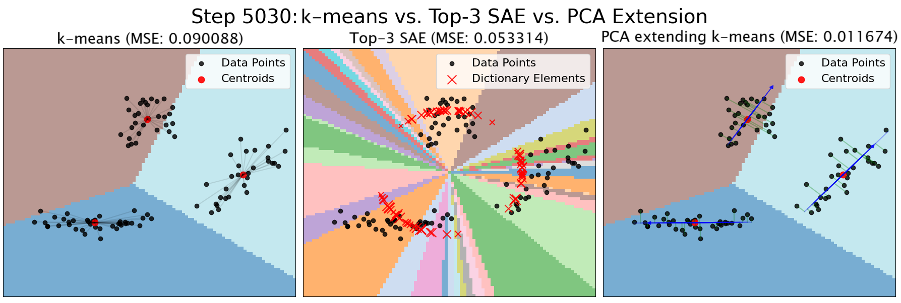
Figure 2: Visualising the SAE bridge between $k$-means clustering and PCA. The cyan/brown boundary intersecting the point cloud (left and right figure) is a visualiser bug.

3 A proximal alternating method (PAM-SGD) for training SAEs

3.1 Convergence theory and the PAM-SGD algorithm

It turns out that for any SAE that has the sort of loss function we have been considering, if we fix the encoding, then learning the decoding reduces to linear least squares regression: the decoding seeks an affine map that sends codes $z^{r}:=\rho(W_{\text{enc}}x^{r}+b_{\text{enc}})$ to $x^{r}$. We can therefore solve for the decoding in closed form, which suggests the idea of training an SAE by alternating between updating our encoding holding the decoding fixed, e.g. by SGD, and then updating our decoding holding the encoding fixed, via the closed form optimum. This dovetails well with the spline theory perspective, as we saw in the previous section that the spline geometry depends entirely on the encoding parameters. Therefore, this alternation can be viewed as (i) updating the SAE spline geometry to better use a given decoding, and then (ii) finding the most accurate decoding given that geometry.

In particular, we will consider the following proximal alternating method with quadratic costs to move, as this has solid theoretical foundations Attouch et al. (2010):

$$(W_{\text{enc}}^{t+1},b_{\text{enc}}^{t+1}) =\operatorname*{argmin}_{W_{\text{enc}},b_{\text{enc}}} \sum_{r=1}^{N}\|W_{\text{dec}}^{t}\rho(W_{\text{enc}}x^{r}+b_{\text{enc}})+b_{\text{dec}}^{t}-x^{r}\|_{2}^{2}+F(W_{\text{enc}},b_{\text{enc}})$$ (3.1a)

$$+\mu_{\text{enc}}^{t}\|W_{\text{enc}}-W_{\text{enc}}^{t}\|_{F}^{2}+\nu_{\text{enc}}^{t}\|b_{\text{enc}}-b_{\text{enc}}^{t}\|_{2}^{2}$$

$$(W_{\text{dec}}^{t+1},b_{\text{dec}}^{t+1}) =\operatorname*{argmin}_{W_{\text{dec}},b_{\text{dec}}} \sum_{r=1}^{N}\|W_{\text{dec}}\rho(W^{t+1}_{\text{enc}}x^{r}+b^{t+1}_{\text{enc}})+b_{\text{dec}}-x^{r}\|_{2}^{2}+G(W_{\text{dec}},b_{\text{dec}})$$ (3.1b)

$$+\mu_{\text{dec}}^{t}\|W_{\text{dec}}-W_{\text{dec}}^{t}\|_{F}^{2}+\nu^{t}_{\text{dec}}\|b_{\text{dec}}-b_{\text{dec}}^{t}\|_{2}^{2}$$

We next use Attouch et al. (2010) to analyse the convergence of Equation˜3.1, and find that under some assumptions (which will require minor adjustments to our SAE settings, see ˜C.2 and C.3) the sequence defined by (3.1) converges to a critical point of the following loss:

$$\mathcal{L}(W_{\text{enc}},b_{\text{enc}},W_{\text{dec}},b_{\text{dec}}):=\sum_{r=1}^{N}\|W_{\text{dec}}\rho(W_{\text{enc}}x^{r}+b_{\text{enc}})+b_{\text{dec}}-x^{r}\|_{2}^{2}+F(W_{\text{enc}},b_{\text{enc}})+G(W_{\text{dec}},b_{\text{dec}}).$$

We summarise the convergence result as follows, for details see Section˜C.1.

The optimal decoding for Equation˜3.1b with weight decay $G:=\alpha\|W_{\text{dec}}\|^{2}_{F}+\beta\|b_{\text{dec}}\|_{2}^{2}$ can still be found in closed form, see Theorem˜C.1. This gives the following novel method for training an SAE by solving Equation˜3.1b exactly, which we call a proximal alternating method SGD (PAM-SGD) algorithm.

3.2 Sample-efficient sparse coding for MNIST and LLMs: PAM-SGD vs. SGD

We performed two experiments comparing the benefits of our PAM-SGD method (Algorithm˜3.1) vs. standard SGD (using Adam for SGD in both cases) for training SAEs: (i) on simple visual domains, using the MNIST dataset, and (ii) on high-dimensional LLM activations, using Google DeepMind’s Gemma-2-2B.

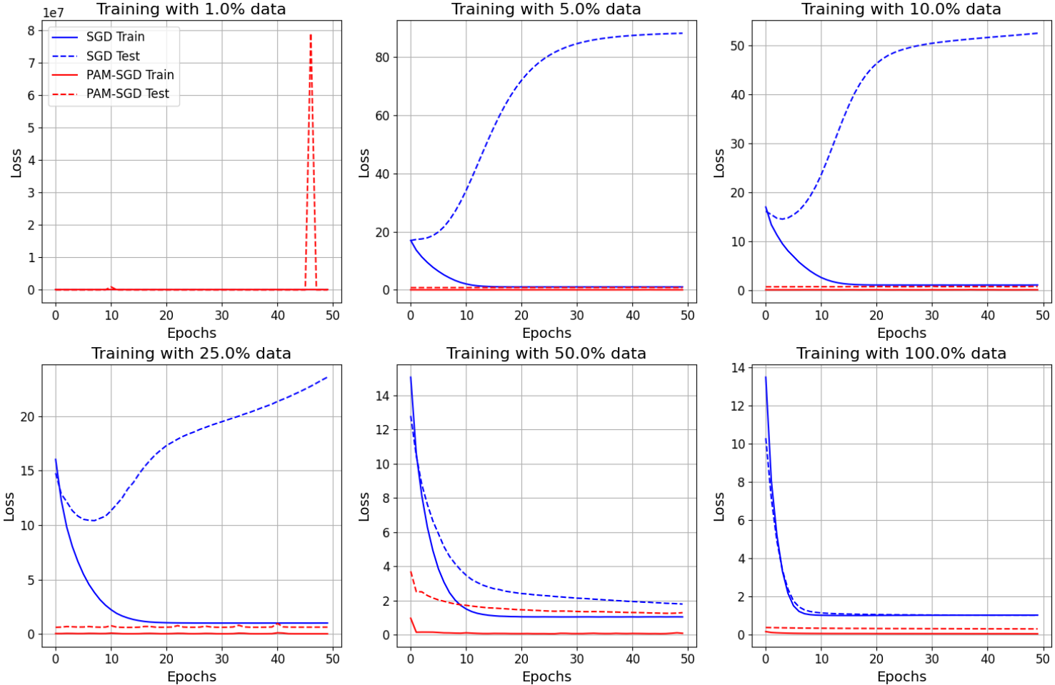
Figure 3: Training and test loss curves at different data sizes for MNIST, with ReLU activation. The chart highlights PAM-SGD’s superior sample efficiency and convergence speed.

For MNIST we used $n=28^{2}$ input dimensions and $d=256$ hidden dimensions. Our LLM experiments used activations from the 12th layer of Gemma-2-2B, with $n=2304$ and a highly overcomplete hidden dimension $d=4096$. Experimental settings are described in Appendix˜D, and additional figures and ablation studies can be found in Appendix˜E.

PAM-SGD generalised better than SGD in low-data regimes. (Figures˜3, 4, 9, 24, 25, 26, 29, 28 and 27)

On MNIST, PAM-SGD consistently (using both ReLU and TopK) substantially outperformed SGD in test loss, especially when trained on just 1%–25% of the MNIST training data. In the LLM experiments, PAM-SGD again outperformed SGD when using ReLU activations, especially for low data. However, PAM-SGD became unstable when TopK was used unless $K$ was large; even for $K=320$ and $K=640$ it underperformed SGD, slightly for low (and high) data and substantially for medium data.

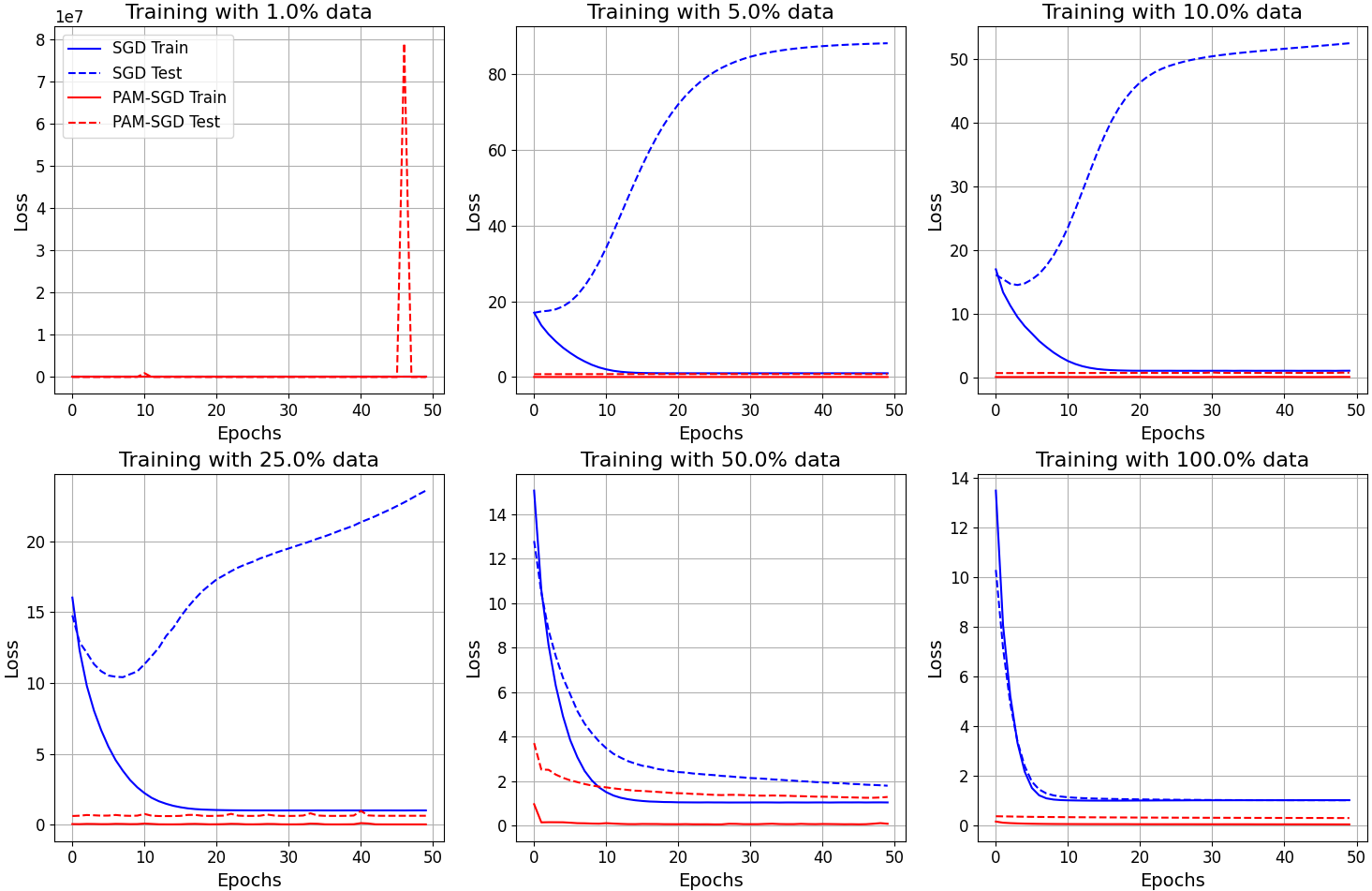
Figure 4: Training and test loss curves at different data sizes for Gemma-2-2B, with ReLU activation. PAM-SGD again has a huge advantage at low data, and remains superior throughout.

PAM-SGD was faster, more accurate, and more interpretable on MNIST. (Figures˜12, 14, 10, 13, 15 and 11)

Reconstruction comparisons over training epochs show that PAM-SGD reconstructions were cleaner and converged faster than those from SGD. This was particularly evident when tracking digit reconstructions over time; PAM-SGD’s exhibited sharper edges and more localised structure by early training. By the end of training, both methods produced visually accurate reconstructions, but PAM-SGD’s showed slightly better fidelity and smoothness, and more closely resembled the originals. Finally, visualizing encoder and decoder filters in the TopK case reveals that both SGD and PAM-SGD learned edge- and stroke-like patterns, but PAM-SGD’s filters were sharper and better structured.

Summary and practical implications.

PAM-SGD demonstrated clear advantages over SGD on MNIST in terms of generalisation, convergence speed, reconstruction quality, and (using TopK) visual interpretability, particularly in low-data regimes. Even in a much more challenging real-world LLM setting, PAM-SGD with ReLU still substantially outperformed in low data, and improved activation sparsity by about 15%. However, issues arose for TopK: small $K$ led to rapidly diverging test loss, and for larger $K$ PAM-SGD still underperformed SGD (though only slightly for low data). In summary, these results suggest that PAM-SGD is a powerful tool for learning overcomplete, sparse representations from visual data and LLM activations in low-data regimes, provided that the sparsity can adapt to the data. This insight is important in downstream applications where data may be scarce.

4 Conclusions and limitations

In this work, we have sought to apply a spline theoretical lens to SAEs, to gain insight into how, why, and whether SAEs work. Given the current prominence of SAEs in mechanistic interpretability, and the societal importance of interpreting AI systems, we hope that the development of SAE theory (and our small contribution to it) can help develop more efficient, fairer, and reliable AI systems.

Building on the piecewise affine spline nature of SAEs, we characterised the spline geometry of TopK SAEs as exactly the $K^{\text{th}}$-order power diagrams, opening the door to directly incorporating geometric constraints into SAEs. We linked SAEs with traditional ML, showing how $k$-means can be viewed as a special kind of SAE, and how SAEs sacrifice accuracy for interpretability vs. the optimal piecewise affine autoencoder, which we showed to be a $k$-means-esque clustering with a local PCA correction. Finally, we developed a new proximal alternating training method (PAM-SGD) for SAEs, with both solid theoretical foundations and promising empirical results, particularly in sample efficiency and activation sparsity for LLMs, two pain points for mechanistic interpretability. PAM-SGD’s separate updating of encoding and decoding dovetails well with the spline theory perspective of the encoding shaping the SAE’s spline geometry vs. the decoding driving the SAE’s autoencoding accuracy.

This work is the beginning of a longer theoretical exploration, and is thus limited in ways we hope to address in future work. Our characterisation of the spline geometry of SAEs is currently limited to TopK SAEs; future work will seek to extend this, and explore more explicitly the incorporation of geometry into SAE training, perhaps giving insight into how to tailor an SAE architecture for a given task. Our bridge between SAEs and PCA-based autoencoders sets aside the matter (see ˜2.7) of shared decoding vectors. Future work will study the optimal autoencoding in that setting, and related results in the superposition hypothesis setting. Finally, PAM-SGD makes approximations which break assumptions of the theory, and had some empirical limitations. Future work will seek to understand more deeply the pros and cons of PAM-SGD, and incorporate the SGD step into the theory.

Appendix A Visualisations of Voronoi and power diagrams

A.1 Spatial Partitioning Methods: From Voronoi to Power Diagrams

This experiment explores the theoretical connections between different spatial partitioning methods. Starting with standard Voronoi diagrams that divide the plane based on proximity to generator points, we demonstrate how they relate to nearest-neighbor classification ($k=1$), centroidal clustering ($k$-means), and finally to power diagrams which introduce weights to Voronoi cells. These relationships reveal that power diagrams emerge as a generalization of Voronoi diagrams, offering additional flexibility through weighted distance metrics and enabling richer geometric representations of data.

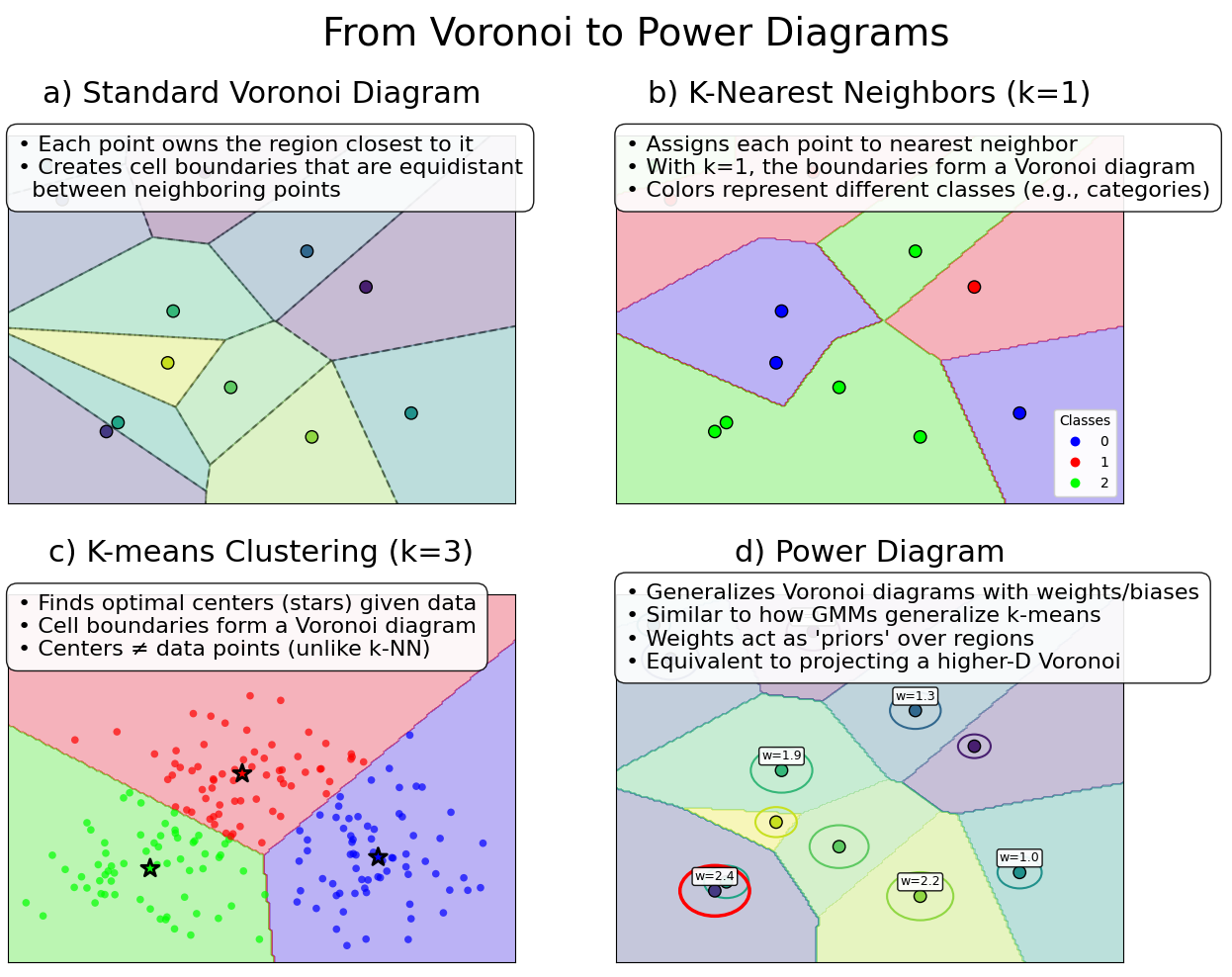
Figure 5: Spatial Partitioning Methods (a) Standard Voronoi diagram where space is partitioned based on the nearest generator point using Euclidean distance; (b) Nearest-neighbor ($k=1$) classification showing how Voronoi cells define decision boundaries for point classification (c) $k$-means clustering with $k=3$ demonstrating how cluster centroids generate Voronoi cells that define cluster boundaries (d) Power diagram (weighted Voronoi) where each generator has an associated weight, creating curved boundaries between regions. Power diagrams generalise Voronoi diagrams and provide additional flexibility for modeling spatial relationships.

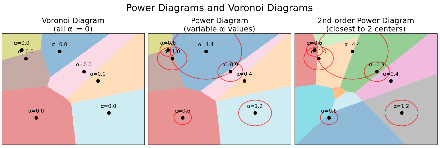
(a)

(b)

Figure 6: Progressive Generalization of Voronoi Diagrams. Comparison showing (left) standard Voronoi diagram, (center) first-order power diagram with linear distance weighting, and (right) second-order power diagram. This progression demonstrates how higher-order power diagrams can capture more sophisticated spatial relationships.

A.2 3D Voronoi diagrams to 2D power diagrams

There is a neat relationship between power diagrams and projections of Voronoi diagrams, observed in Ash & Bolker (1986). Suppose that we consider a Vononoi diagram in $n+1$ dimensions with cells defined by centroids $\{(\mu_{i},\zeta_{i})\}_{i=1}^{k}\in\mathbb{R}^{n+1}$, i.e. the $i^{\text{th}}$ cell is defined to be

$$C_{i}:=\{(x,z)\in\mathbb{R}^{n+1}:\|(x,z)-(\mu_{i},\zeta_{i})\|_{2}^{2}<\|(x,z)-(\mu_{j},\zeta_{j})\|_{2}^{2}\text{ for all }j\neq i\}.$$

Now suppose that we project this diagram into $n$-dimensional space, for example defining

$$\hat{C}_{i}:=\{x\in\mathbb{R}^{n}:(x,0)\in C_{i}\}=\{x\in\mathbb{R}^{n}:\|x-\mu_{i}\|_{2}^{2}+\zeta_{i}^{2}<\|x-\mu_{j}\|_{2}^{2}+\zeta_{j}^{2}\text{ for all }j\neq i\}.$$

This is precisely a power diagram with centroids $\{\mu_{i}\}_{i=1}^{k}\in\mathbb{R}^{n}$ (the projections of the Voronoi centroids) and weights $\alpha_{i}=-\zeta_{i}^{2}$. Conversely, for any power diagram defined by centroids $\{\mu_{i}\}_{i=1}^{k}\in\mathbb{R}^{n}$ and weights $\{\alpha_{i}\}_{i=1}^{k}\in\mathbb{R}$, we can subtract a constant from the $\alpha_{i}$ to get an equivalent power diagram with all non-positive weights, and therefore compute $\zeta_{i}$ such that the corresponding Voronoi diagram with centroids $\{(\mu_{i},\zeta_{i})\}_{i=1}^{k}\in\mathbb{R}^{n+1}$ projects to that power diagram. We visualise this mathematical relationship between 3D Voronoi diagrams and 2D power diagrams in Figure˜7.

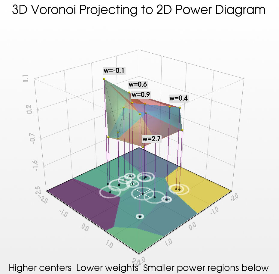
(a)

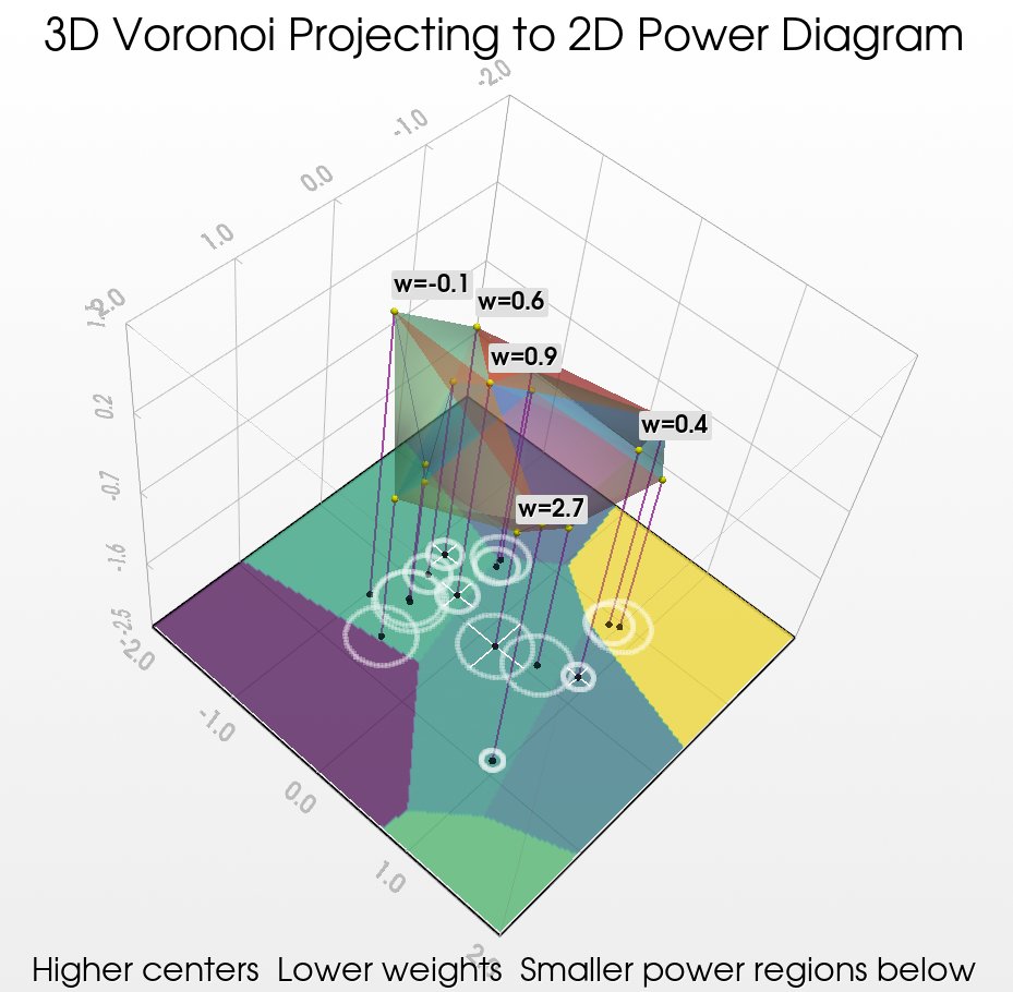
(b)

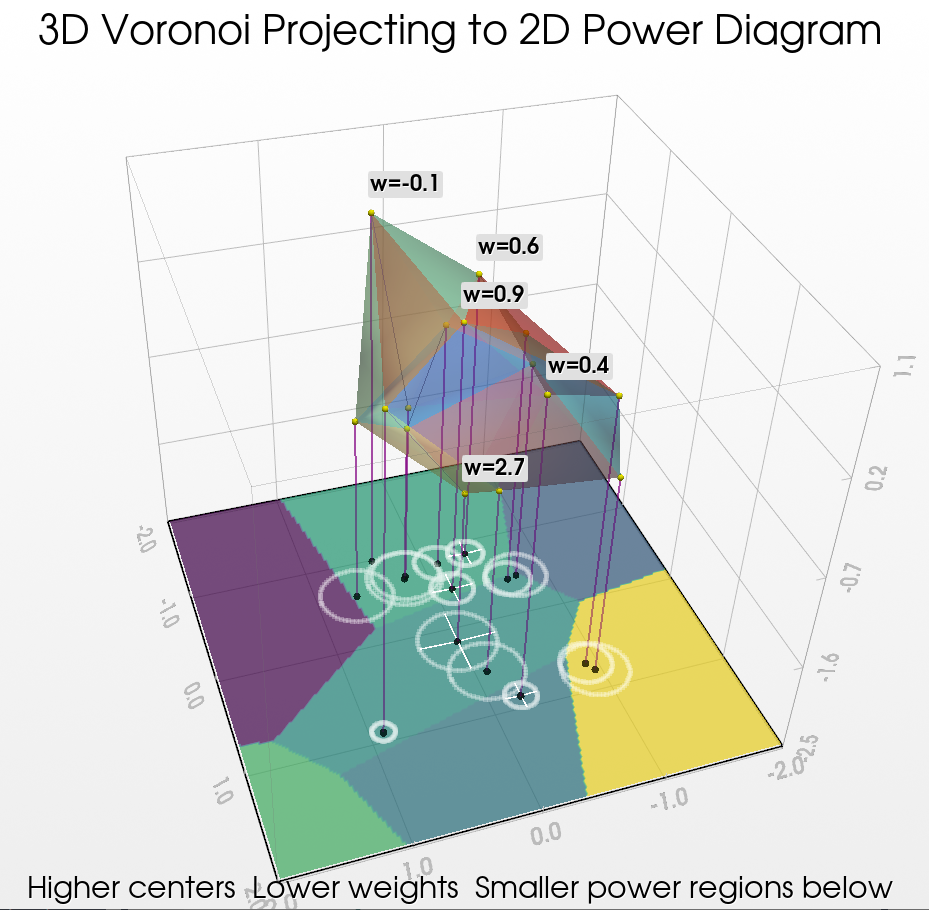
(c)

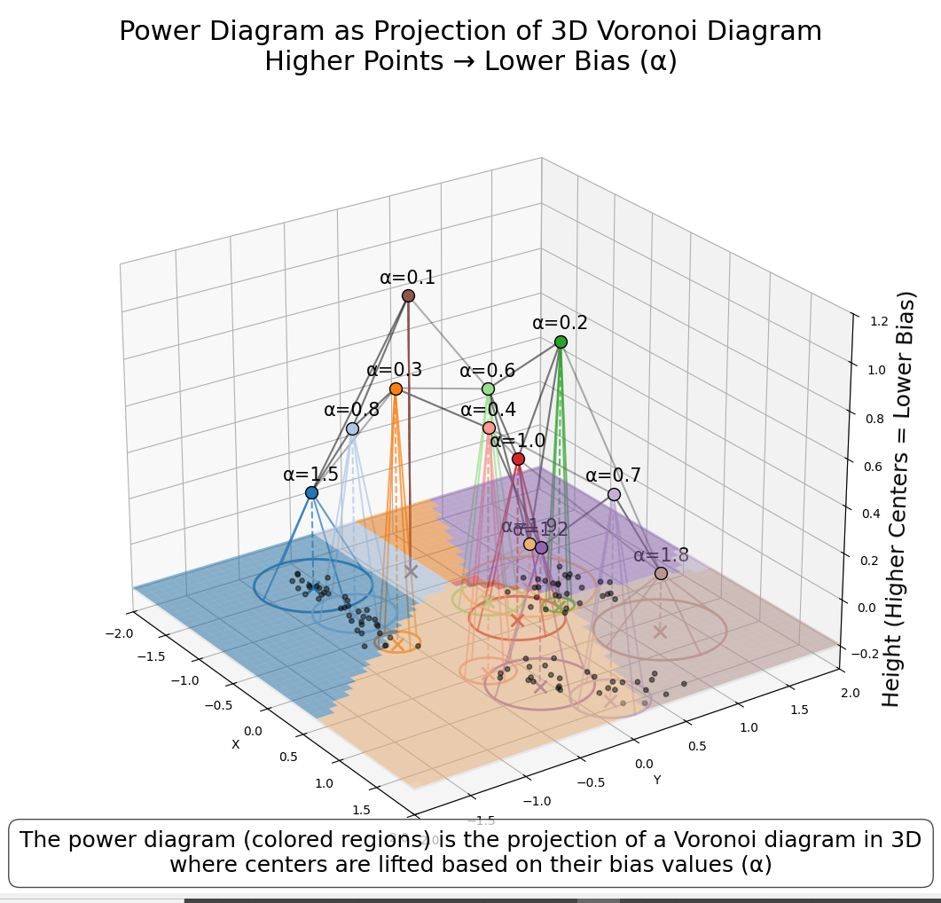
(d)

Figure 7: Projection of 3D Voronoi diagrams onto 2D power diagrams. The resulting power cells demonstrate the preservation of topological structure through projection

Appendix B Proofs in Section˜2

Proof of Theorem˜B.1.

The forms of $H$ and $c$ can be immediately derived by rearranging the inequalities in the definitions of $\Omega^{\operatorname{JumpReLU}}_{S}$ and $\Omega_{S}^{\operatorname{TopK}}$. Convexity immediately follows, since if $Hx_{1}>c$ and $Hx_{2}>c$, then for all $t\in[0,1]$

$$H(tx_{1}+(1-t)x_{2})=tHx_{1}+(1-t)Hx_{2}>tc+(1-t)c=c.$$

Finally, suppose that $x\in\mathbb{R}^{n}$ lies in the interior of $\{x:Hx\geq c\}$. That is, there exists $\varepsilon>0$ such thatr for all $\eta\in\mathbb{R}^{n}$ with $\|\eta\|_{2}<\varepsilon$, $H(x+\eta)\geq c$. We wish to show that $Hx>c$.

Suppose not, then for some $j$, $(Hx)_{j}=c_{j}$. Therefore for all $\eta\in\mathbb{R}^{n}$ with $\|\eta\|_{2}<\varepsilon$, $(H\eta)_{j}\geq 0$, and therefore for all $\eta\in\mathbb{R}^{n}$, $(H\eta)_{j}=0$. This is possible if and only if the $j^{\text{th}}$ row of $H$ is all zeroes. In the JumpReLU case, the $j^{\text{th}}$ row of $H$ is $\pm$ the $j^{\text{th}}$ row of $W_{\text{enc}}$ (depending on if $j\in S$ or $j\notin S$) and hence is zero if and only if the the $j^{\text{th}}$ row of $W_{\text{enc}}$ is zero. In the TopK case, the $(i,j)^{\text{th}}$ row of $H$ is the difference between the $i^{\text{th}}$ and $j^{\text{th}}$ rows of $W_{\text{enc}}$, which is zero if and only if those rows are identical. ∎

Proof of Theorem˜B.2.

Define the power functions

$$P_{i}(x):=-2\mu_{i}^{T}x+\|\mu_{i}\|^{2}_{2}-\alpha_{i} Q_{S}(x):=-2\nu_{S}^{T}x+\|\nu_{S}\|^{2}_{2}-\beta_{S}.$$ and

Then by subtracting $\|x\|_{2}^{2}$ from both sides of the defining inequalities we get:

$$C_{S} =\{x:P_{i}(x)<P_{j}(x)\text{ for all $i\in S$, and $j\in S^{c}$}\},$$

$$R_{S} =\{x:Q_{S}(x)<Q_{T}(x)\text{ for all $T\neq S$, $T$ a $K$-subset of $\{1,...,k\}$}\}.$$

It is straightforward to check that

$$Q_{S}(x)=\frac{1}{K}\sum_{i\in S}P_{i}(x),$$

and hence

$$x\in R_{S}\text{ if and only if }\sum_{i\in S}P_{i}(x)<\sum_{i\in T}P_{i}(x)\text{ for all $T\neq S$ a $K$-subset}.$$

Suppose that $x\in R_{S}$, and let $i\in S$ and $j\in S^{c}$. Let $T=(S\setminus\{i\})\cup\{j\}$. This is a $K$-subset distinct from $S$, and so

$$P_{i}(x)+\sum_{k\in S\setminus\{i\}}P_{k}(x)=\sum_{i\in S}P_{i}(x)<\sum_{i\in T}P_{i}(x)=P_{j}(x)+\sum_{k\in S\setminus\{i\}}P_{k}(x)$$

and hence $P_{i}(x)<P_{j}(x)$. Hence $x\in C_{S}$.

Now suppose that $x\in C_{S}$ and let $T\neq S$ be a $K$-subset. Then

$$\sum_{i\in S}P_{i}(x)=\sum_{i\in S\cap T}P_{i}(x)+\sum_{i\in S\setminus T}P_{i}(x)<\sum_{i\in S\cap T}P_{i}(x)+\sum_{j\in T\setminus S}P_{j}(x)=\sum_{i\in T}P_{i}(x)$$

where we have used that $|S\setminus T|=|T\setminus S|$ and for each $i\in S\setminus T$ and $j\in T\setminus S$, $P_{i}(x)<P_{j}(x)$. Hence $x\in R_{S}$. ∎

Proof of ˜2.2.

Identify $\mathbb{R}^{2}$ with $\mathbb{C}$. Then we would need $\{\mu_{i}\}_{i=1}^{4}\in\mathbb{C}$ such that

$$\nu_{12}=1 =\frac{1}{2}\mu_{1}+\frac{1}{2}\mu_{2}, \nu_{13}=e^{\pi i/3} =\frac{1}{2}\mu_{1}+\frac{1}{2}\mu_{3},$$

$$\nu_{14}=e^{2\pi i/3} =\frac{1}{2}\mu_{1}+\frac{1}{2}\mu_{4}, \nu_{23}=-1 =\frac{1}{2}\mu_{2}+\frac{1}{2}\mu_{3},$$

$$\nu_{24}=-e^{\pi i/3} =\frac{1}{2}\mu_{2}+\frac{1}{2}\mu_{4}, \nu_{34}=-e^{2\pi i/3} =\frac{1}{2}\mu_{3}+\frac{1}{2}\mu_{4}.$$

Hence $\mu_{2}-\mu_{4}=(\frac{1}{2}\mu_{1}+\frac{1}{2}\mu_{2})+(\frac{1}{2}\mu_{2}+\frac{1}{2}\mu_{3})-(\frac{1}{2}\mu_{1}+\frac{1}{2}\mu_{4})-(\frac{1}{2}\mu_{3}+\frac{1}{2}\mu_{4})=1+(-1)-e^{2\pi i/3}-(-e^{2\pi i/3})=0$, so $\mu_{2}=\mu_{4}$ and hence $1=\frac{1}{2}\mu_{1}+\frac{1}{2}\mu_{2}=\frac{1}{2}\mu_{1}+\frac{1}{2}\mu_{4}=e^{2\pi i/3}$, a contradiction. ∎

Proof of Theorem˜2.3.

For each $S$, $\Omega^{\operatorname{TopK}}_{S}$ is given by

$$\Omega^{\operatorname{TopK}}_{S}=\{x\in\mathbb{R}^{n}:e_{i}^{T}W_{enc}x+(b_{enc})_{i}>e_{j}^{T}W_{enc}x+(b_{enc})_{j}\text{ for all $i\in S$ and $j\in S^{c}$}\}.$$

We can rewrite the definition of $C_{S}$ in a $K^{\text{th}}$-order power diagram as

$$C_{S}:=\{x\in\mathbb{R}^{n}:\mu_{i}^{T}x+\frac{1}{2}\alpha_{i}-\frac{1}{2}\|\mu_{i}\|_{2}^{2}>\mu_{j}^{T}x+\frac{1}{2}\alpha_{j}-\frac{1}{2}\|\mu_{j}\|_{2}^{2}\text{ for all $i\in S$ and $j\in S^{c}$}\}.$$

It follows that $\Omega^{\operatorname{TopK}}_{S}=C_{S}$ if for all $\ell$

$$e^{T}_{\ell}W_{enc}=\mu_{\ell}^{T} (b_{enc})_{\ell}=\frac{1}{2}\alpha_{\ell}-\frac{1}{2}\|\mu_{\ell}\|_{2}^{2},$$ and i.e.

$$\mu_{\ell}=W^{T}_{enc}e_{\ell} \alpha_{\ell}=2(b_{enc})_{\ell}+\|W^{T}_{enc}e_{\ell}\|_{2}^{2}.$$ and

Hence, any $(W_{enc},b_{enc})$ gives rise to a $K^{\text{th}}$-order power diagram, and any $K^{\text{th}}$-order power diagram gives rise to an $(W_{enc},b_{enc})$. Finally, Equation˜2.2 follows from Equation˜B.1 and Equation˜2.1. ∎

Proof of Theorem˜2.6.

We seek to minimise

$$\mathcal{L}=\sum_{i=1}^{k}\lambda N_{i}K_{i}+\sum_{x^{r}\in R_{i}}\|x^{r}-U_{i}V_{i}^{T}x^{r}-c_{i}\|_{2}^{2}.$$

For the same reason as for the $\nu_{i}$ in $k$-means, the $c_{i}$ will be minimising when

$$c_{i}=\frac{1}{N_{i}}\sum_{x^{r}\in R_{i}}(I-U_{i}V_{i}^{T})x^{r}=(I-U_{i}V_{i}^{T})\bar{x}_{i},$$

and so $\mathcal{L}$ simplifies to

$$\mathcal{L}=\sum_{i=1}^{k}\lambda N_{i}K_{i}+\sum_{x^{r}\in R_{i}}\|(I-U_{i}V_{i}^{T})(x^{r}-\bar{x}_{i})\|_{2}^{2}.$$

We claim that this is minimised when $U_{i}=V_{i}$ and the columns of $U_{i}$ are the top $K_{i}$ eigenvectors of

$$X_{i}:=\frac{1}{N_{i}}\sum_{x^{r}\in R_{i}}(x^{r}-\bar{x}_{i})(x^{r}-\bar{x}_{i})^{T},$$

and in this case $\mathcal{L}$ reduces to

$$\mathcal{L}=\sum_{i=1}^{k}\lambda N_{i}K_{i}+\left(\sum_{x^{r}\in R_{i}}\|(x^{r}-\bar{x}_{i})\|_{2}^{2}\right)-N_{i}\sum_{\ell=1}^{K_{i}}\lambda_{\ell}(X_{i}),$$

where $\lambda_{\ell}(X_{i})$ are the eigenvalues of $X_{i}$ in descending order.

This follows because

$$\sum_{x^{r}}\|(I-UV^{T})(x^{r}-\bar{x})\|_{2}^{2} =\sum_{x^{r}}(x^{r}-\bar{x})^{T}(I-VU^{T})(I-UV^{T})(x^{r}-\bar{x})$$

$$=\sum_{x^{r}}\operatorname{tr}\left((x^{r}-\bar{x})^{T}(I-VU^{T})(I-UV^{T})(x^{r}-\bar{x})\right)$$

$$=\sum_{x^{r}}\operatorname{tr}\left((x^{r}-\bar{x})(x^{r}-\bar{x})^{T}(I-VU^{T})(I-UV^{T})\right)$$

$$=N\operatorname{tr}\left(X(I-VU^{T})(I-UV^{T})\right)$$

$$=N\operatorname{tr}\left((X-XVU^{T})(I-UV^{T})\right)$$

$$=N\operatorname{tr}\left(X-XVU^{T}-XUV^{T}+XVV^{T}\right)$$

$$=N\operatorname{tr}(X)+N\operatorname{tr}\left(-U^{T}XV-V^{T}XU+V^{T}XV\right)$$

$$=N\operatorname{tr}(X)+N\operatorname{tr}\left((V-U)^{T}X(V-U)\right)-N\operatorname{tr}\left(U^{T}XU\right)$$

is minimised when $U=V$ and $\operatorname{tr}\left(U^{T}XU\right)$ is maximised (with the constraint that $U^{T}U=I$). This occurs when $U$ has columns the top $K$ leading eigenvectors of $X$. At this choice:

$$\sum_{x^{r}}\|(I-UV^{T})(x^{r}-\bar{x})\|^{2}=N\operatorname{tr}(X)-N\sum_{\ell=1}^{k}\lambda_{\ell}=\sum_{x^{r}}\operatorname{tr}((x^{r}-\bar{x})^{T}(x^{r}-\bar{x}))-N\sum_{\ell=1}^{k}\lambda_{\ell}=\sum_{x^{r}}\|x^{r}-\bar{x}\|_{2}^{2}-N\sum_{\ell=1}^{k}\lambda_{\ell}.$$

∎

Appendix C Proofs in Section˜3

Proof of Theorem˜C.1.

By completing the square, the optimal $b_{\text{dec}}$ is given by

$$b_{\text{dec}}=\frac{1}{N+\beta+\nu^{t}_{\text{dec}}}\left(\nu^{t}_{\text{dec}}b_{\text{dec}}^{t}+\sum_{r=1}^{t}x^{r}-W_{\text{dec}}z_{t+1}^{r}\right)=\frac{\nu^{t}_{\text{dec}}}{N+\beta+\nu^{t}_{\text{dec}}}b_{\text{dec}}^{t}+\frac{N}{N+\beta+\nu^{t}_{\text{dec}}}(\bar{x}-W_{\text{dec}}\bar{z}_{t+1}),$$

where

$$z^{r}_{t+1}:=\rho(W^{t+1}_{\text{enc}}x^{r}+b^{t+1}_{\text{enc}}) \bar{z}_{t+1}:=\frac{1}{N}\sum_{r=1}^{N}z^{r}_{t+1}.$$ and

This reduces $\mathcal{L}$ to:

$$\sum_{r=1}^{N}\left\|W_{\text{dec}}\left(z^{r}_{t+1}-\frac{N}{N+\beta+\nu^{t}_{\text{dec}}}\bar{z}_{t+1}\right)+\frac{\nu^{t}_{\text{dec}}}{N+\beta+\nu^{t}_{\text{dec}}}b_{\text{dec}}^{t}+\frac{N}{N+\beta+\nu^{t}_{\text{dec}}}\bar{x}-x^{r}\right\|_{2}^{2}$$

$$+\mu_{\text{dec}}^{t}\|W_{\text{dec}}-W_{\text{dec}}^{t}\|_{F}^{2}+\alpha\|W_{\text{dec}}\|^{2}_{F}+\nu^{t}_{\text{dec}}\left\|\frac{N}{N+\beta+\nu^{t}_{\text{dec}}}(\bar{x}-W_{\text{dec}}\bar{z}_{t+1})-\frac{N+\beta}{N+\beta+\nu^{t}_{\text{dec}}}b_{\text{dec}}^{t}\right\|_{2}^{2}$$

$$+\beta\left\|\frac{\nu^{t}_{\text{dec}}}{N+\beta+\nu^{t}_{\text{dec}}}b_{\text{dec}}^{t}+\frac{N}{N+\beta+\nu^{t}_{\text{dec}}}(\bar{x}-W_{\text{dec}}\bar{z}_{t+1})\right\|_{2}^{2}.$$

Hence

$$\mathcal{L} =\sum_{r=1}^{N+2}\|W_{\text{dec}}\psi_{t}^{r}-\phi_{t}^{r}\|^{2}_{2}+\mu_{\text{dec}}^{t}\|W_{\text{dec}}-W_{\text{dec}}^{t}\|_{F}^{2}+\alpha\|W_{\text{dec}}\|^{2}_{F}$$

$$=\|W_{\text{dec}}\Psi_{t}-\Phi_{t}\|_{F}^{2}+\mu_{\text{dec}}^{t}\|W_{\text{dec}}-W_{\text{dec}}^{t}\|_{F}^{2}+\alpha\|W_{\text{dec}}\|^{2}_{F}$$

$$=\left\|W_{\text{dec}}\begin{pmatrix}\Psi_{t}&\sqrt{\mu^{t}_{\text{dec}}}I_{d}&\sqrt{\alpha}I_{d}\end{pmatrix}-\begin{pmatrix}\Phi_{t}&\sqrt{\mu^{t}_{\text{dec}}}W^{t}_{\text{dec}}&0_{n\times d}\end{pmatrix}\right\|_{F}^{2}$$

and so

$$W_{\text{dec}} =\begin{pmatrix}\Phi_{t}&\sqrt{\mu^{t}_{\text{dec}}}W^{t}_{\text{dec}}&0_{n\times d}\end{pmatrix}\begin{pmatrix}\Psi_{t}&\sqrt{\mu^{t}_{\text{dec}}}I_{d}&\sqrt{\alpha}I_{d}\end{pmatrix}^{\dagger}$$

$$=(\Phi_{t}\Psi_{t}^{T}+\mu^{t}_{\text{dec}}W^{t}_{\text{dec}})\left(\Psi_{t}\Psi_{t}^{T}+(\alpha+\mu^{t}_{\text{dec}})I_{d}\right)^{-1}.$$

∎

C.1 Convergence proof

We will need to make the following assumptions.

Proof of ˜C.3.

It is straightforward to check that if $\rho$ is smooth and (real) analytic, then the $\rho$-dependent conditions of ˜C.2 will be satisfied.

As for the convergence of $\rho_{T}$ to $\operatorname{TopK}$, let $v$ have a unique set of $K$ largest entries, and denote this set $S^{*}$. Then multiplying the numerator and denominator by $\exp\left(-\frac{1}{T}\sum_{j\in S^{*}}v_{j}\right)$ we get that

$$\rho_{T}(v)=\sum_{S\subseteq\{1,...,d\},|S|=K}\frac{\exp\left(\frac{1}{T}\left[\sum_{j\in S}v_{j}-\sum_{j\in S^{*}}v_{j}\right]\right)}{1+\sum_{S^{\prime}\neq S^{*}}\exp\left(\frac{1}{T}\left[\sum_{j\in S^{\prime}}v_{j}-\sum_{j\in S^{*}}v_{j}\right]\right)}P_{S}v.$$

As $T\to 0$, if $S\neq S^{*}$ then $\exp\left(\frac{1}{T}\left[\sum_{j\in S}v_{j}-\sum_{j\in S^{*}}v_{j}\right]\right)\to 0$, since $\sum_{j\in S}v_{j}-\sum_{j\in S^{*}}v_{j}$ is stricly negative. Hence, as $T\to 0$

$$\rho_{T}(v)\to P_{S^{*}}v=\operatorname{TopK}(v).$$

∎

The theory in Attouch et al. (2010) relies crucially on the Kurdyka–Łojasiewicz property, which we now define.

Proof.

Since $\mathcal{L}$ is continuous and piecewise analytic with finitely many pieces, it follows that it is semi-analytic (see Łojasiewicz (1964)). Then if $(W_{\text{enc}},b_{\text{enc}},W_{\text{dec}},b_{\text{dec}})$ is not a critical point of $\mathcal{L}$, the result follows by (Li & Pong, 2017, Lemma 2.1), and if $(W_{\text{enc}},b_{\text{enc}},W_{\text{dec}},b_{\text{dec}})$ is a critical point, the result follows by (Bolte et al., 2007, Theorem 3.1). ∎

We therefore prove a more detailed version of Theorem˜3.1.

Proof.

(i) and (ii) follow from (Attouch et al., 2010, Lemma 3.1). (iii) follows from (Attouch et al., 2010, Proposition 3.1). (iv) and (v) follow from Theorem˜C.5 and (Attouch et al., 2010, Theorem 3.2). (vi) to (viii) follow from Theorem˜C.5 and (Attouch et al., 2010, Theorem 3.4). ∎

Appendix D Experimental settings

All computations were performed on: WS Obsidian 750D AirFlow / AMD Ryzen 9 3900X 12x3.8 Ghz / 2x32GB DDR4 3600 / X570 WS / DIS. NOCTUA / 1000W Platinum / 2TB NVME Ent. / RTX 3090 24GB.

All code is available at: https://github.com/splInterp2025/splInterp.

D.1 SAEs as a bridge between $k$-means and PCA

• Data sampling: 100 points in 2D, sampled as three clusters:

  • 40% on a noisy horizontal line ($x$ from $-1.5$ to $0$, $y\approx-0.8$)

  • 30% in a dense square ($x\in[-0.4,0.4]$, $y\in[0.4,1.2]$)

  • 30% along a noisy diagonal ($x\approx 0.8+t$, $y\approx t-0.5$, $t\in[0,1]$)

• Number of data points: 100

• SAE architecture: Linear sparse autoencoder with 80 dictionary elements ($d=80$), 2D input/output, using a Top1 or Top3 sparse coding.

• Training method and hyperparameters:

  • Adam optimiser (learning rate $8\times 10^{-3}$)

  • 5000 steps, full-batch (all data at once)

  • Dictionary initialised near data points

• Runtime: 6 minutes

D.2 PAM-SGD vs. SGD on MNIST

• Number of data points and training/test split: Uses the standard MNIST dataset:

  • 60,000 training images

  • 10,000 test images

  • Images are $28\times 28$ grayscale digits

• SAE architecture(s): Two models:

  • SGD Autoencoder: Linear encoder/decoder, tied weights, sparsity via TopK ($K=15$) or ReLU (without L1 regularisation), 256 latent dimensions

  • PAM-SGD Autoencoder: Linear encoder, decoder weights solved analytically (not tied), same latent size and sparsity.

• Training (hyper)parameters:

  • Optimiser: Adam (learning rate $0.003$)

  • Batch size: 128 (SGD), 1024 (PAM-SGD encoder update)

  • Number of epochs: 50 (default, or fewer for small ablation subsets)

  • $K$-sparsity: $K=15$ (for TopK)

  • L1 regularisation: not used

  • Input dimension: 784 ($28\times 28$)

  • Ablation studies vary training set size, $K$-sparsity, number of SGD steps per batch, activation type, weight decay parameters, and cost-to-move parameters.

• Running time: 1.5 to 2 hours

D.3 PAM-SGD vs. SGD on Gemma

• Details on Gemma version and license: Uses activations from Gemma-2-2B (https://huggingface.co/google/gemma-2-2b) (Google, 2.2B parameters). License: see Gemma Terms of Use (https://ai.google.dev/gemma/terms) (accessed 8th May 2025).

• Number of data points and training/test split: Up to 10,000 LLM activation vectors extracted from real text (default: 90% train, 10% test split).

• SAE architecture(s): Two models:

  • SGD Autoencoder: Linear encoder/decoder (tied weights), 4096 latent dimensions, sparsity via TopK ($K=320$) or ReLU, with L1 regularisation and “cost-to-move” penalties.

  • PAM-SGD Autoencoder: Linear encoder, decoder weights solved analytically (not tied), same latent size and sparsity, with additional regularisation.

• Training (hyper)parameters:

  • Optimiser: Adam (learning rate $0.001$)

  • Batch size: 256 (SGD), 2048 (PAM-SGD Encoder update)

  • Epochs: 100

  • $K$-sparsity: $K=320$ (for TopK)

  • L1 regularisation: $0.01$ (TopK), $0.00001$ (ReLU)

  • “Cost-to-move” and weight decay regularisation for encoder/decoder

  • Ablation studies vary training set size, $K$-sparsity, number of SGD steps per batch, activation type, weight decay parameters, and cost-to-move parameters.

• Runtimes: 3 to 7 minutes

Appendix E Additional figures and ablation studies

E.1 SAEs as a bridge between $k$-means and PCA

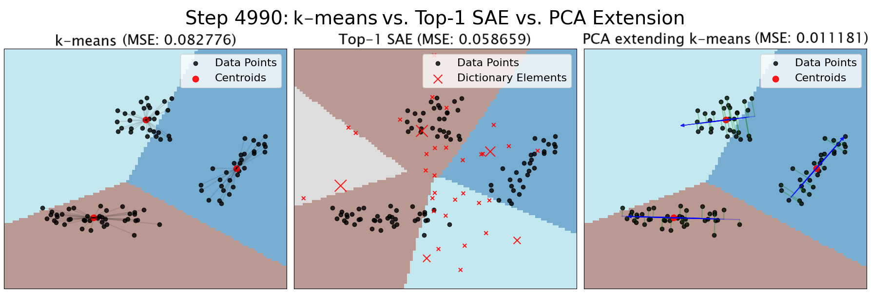
Figure 8: Visualising the SAE bridge between $k$-means clustering and PCA. Top-1 SAE.

E.2 MNIST experiments

E.2.1 TopK experiments

PAM-SGD similarly outperforms SGD with TopK. (Figure˜9)

We tested PAM-SGD using TopK activation for $K=15$. We again saw PAM-SGD outperform SGD, especially at low training data levels.

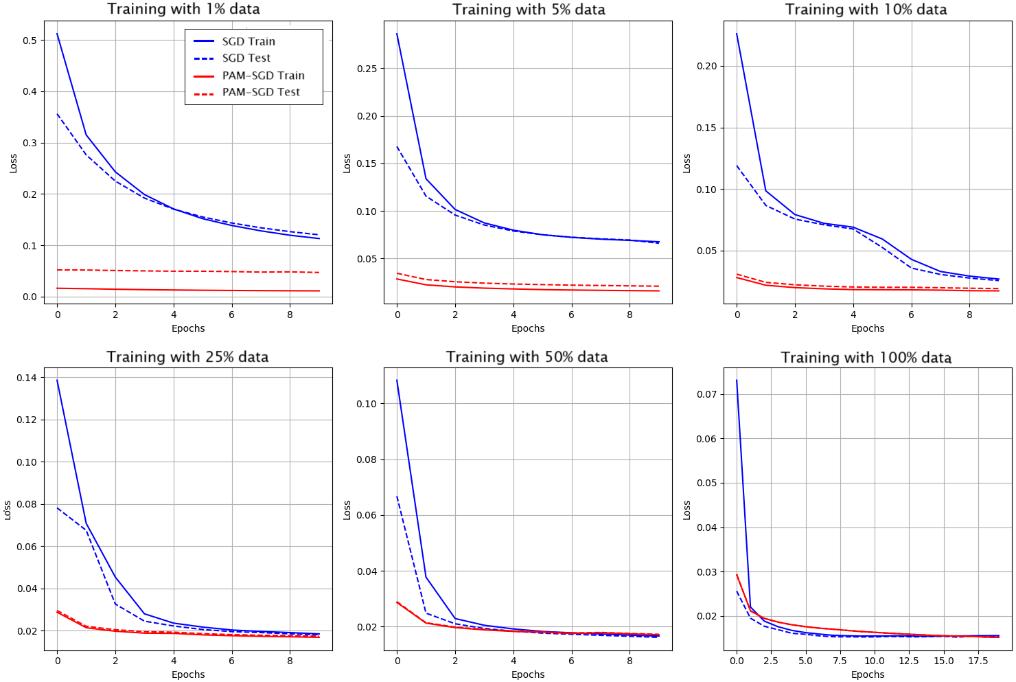
Figure 9: Training and test loss curves at different data sizes for MNIST, with TopK ($K=15$) activation. The chart highlights PAM-SGD’s superior sample efficiency.

E.2.2 Reconstruction accuracy and interpretability

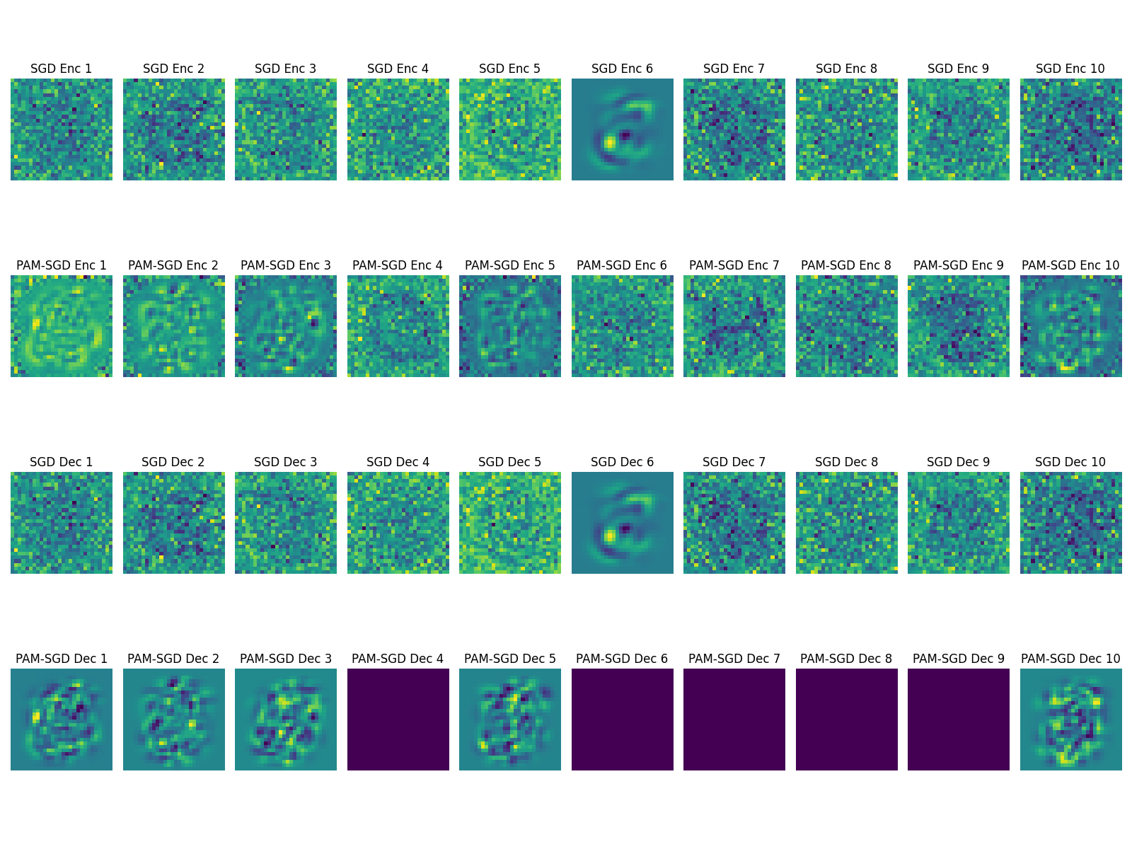
Figure 10: Learned Dictionary Elements using ReLU. Visualization of encoder and decoder weights as filters: SGD encoder (top row), PAM-SGD encoder (second row), SGD decoder (third row), and PAM-SGD decoder (bottom row).

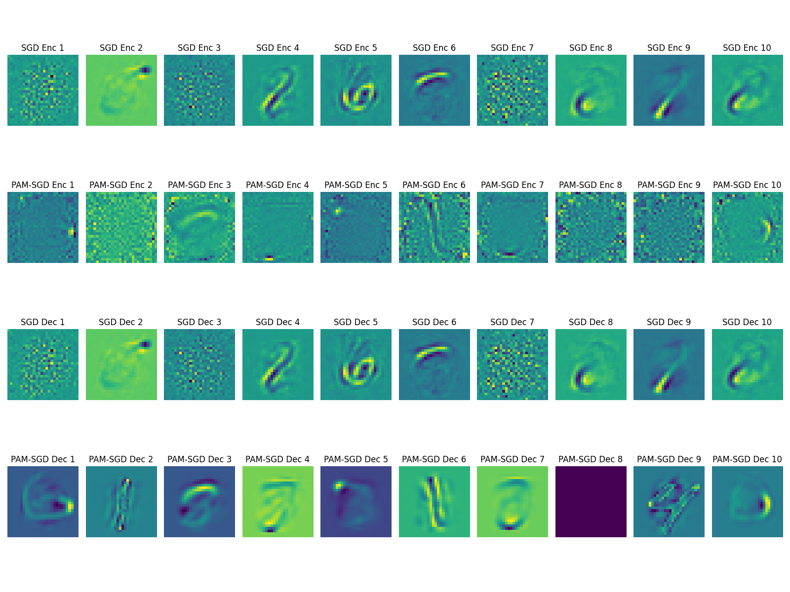
Figure 11: Learned Dictionary Elements using TopK $K=15$. Visualization of encoder and decoder weights as filters: SGD encoder (top row), PAM-SGD encoder (second row), SGD decoder (third row), and PAM-SGD decoder (bottom row). With TopK, PAM-SGD produces more interpretable features representative of digit components

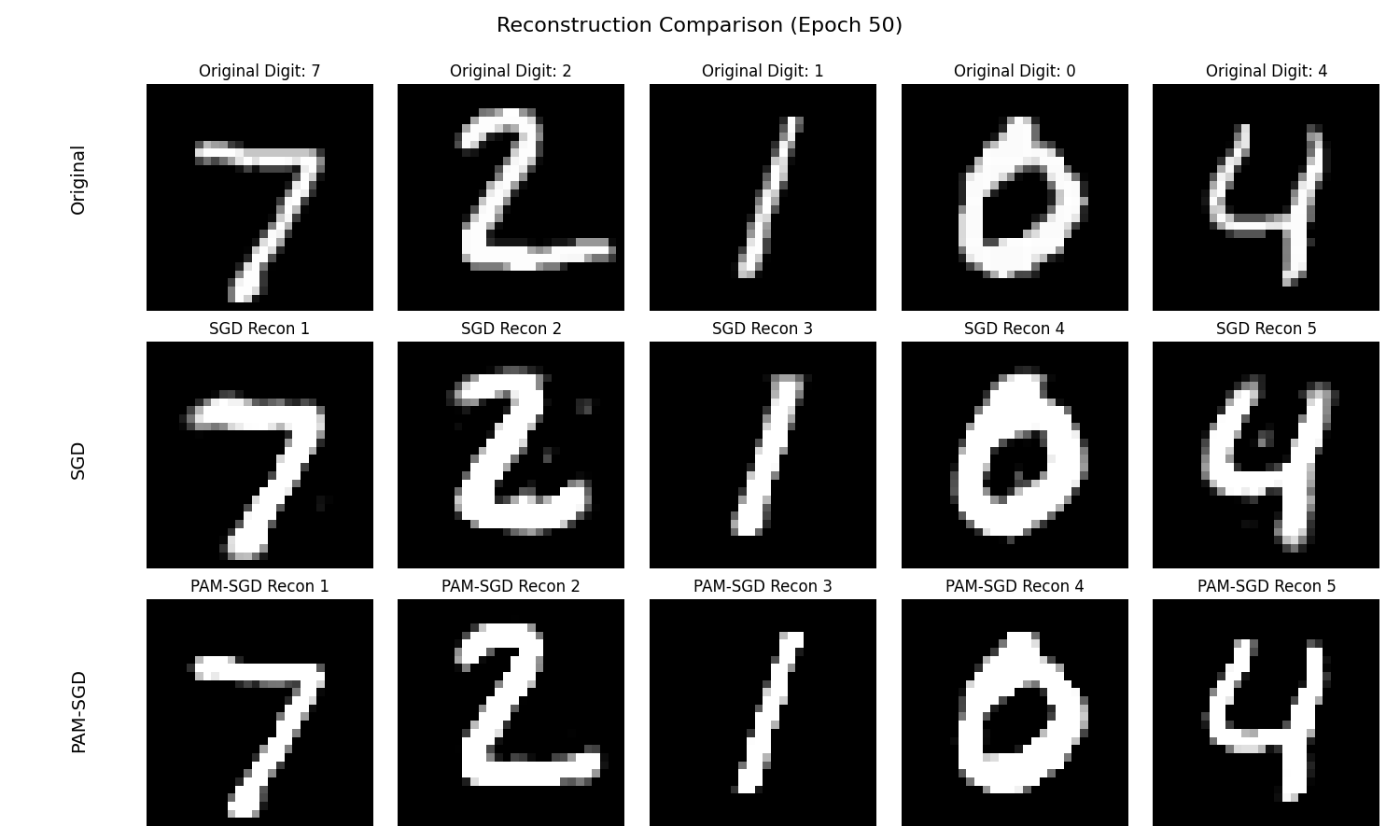
Figure 12: Reconstruction Quality Comparison using ReLU. Original MNIST digits (top row) with their reconstructions using SGD optimization (middle row) and PAM-SGD optimization (bottom row). PAM-SGD produces cleaner, more accurate reconstructions.

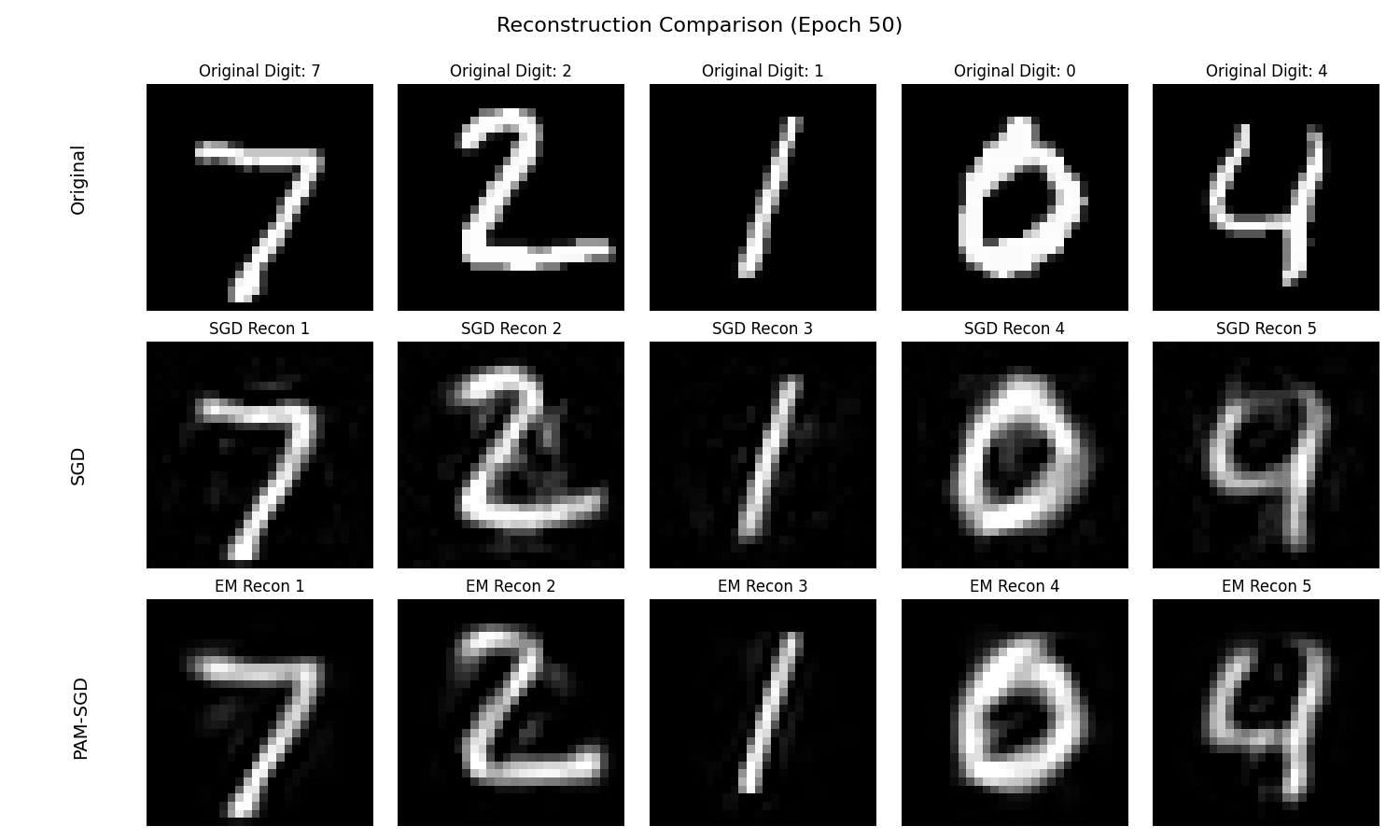
Figure 13: Reconstruction Quality Comparison using TopK $K=15$. Original MNIST digits (top row) with their reconstructions using SGD optimization (middle row) and PAM-SGD optimization (bottom row). PAM-SGD produces cleaner, more accurate reconstructions.

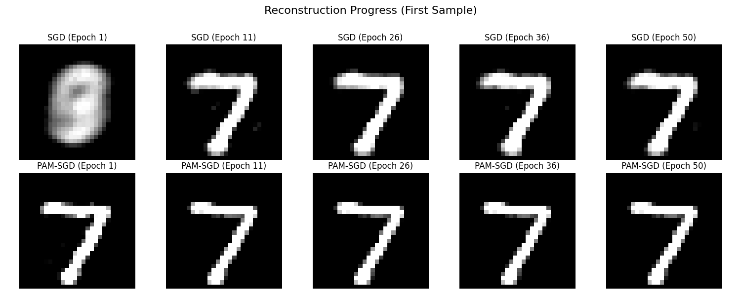
Figure 14: Evolution of Reconstruction Quality Over Training using ReLU. Progression of a single digit’s reconstruction across epochs, comparing SGD (top row) and PAM-SGD (bottom row) approaches, showing how representation quality improves with training. Here PAM-SGD converges almost immediately.

Figure 15: Evolution of Reconstruction Quality Over Training using TopK $K=15$. Progression of a single digit’s reconstruction across epochs, comparing SGD (top row) and PAM-SGD (bottom row) approaches, showing how representation quality improves with training

E.2.3 Ablation study varying SGD updates per batch in PAM-SGD

Stability Across SGD Updates. (Figures˜16 and 17)

Unlike in LLM experiments, PAM-SGD on MNIST is robust to the number of SGD updates per batch. Varying this hyperparameter from 1 to 10 has slightly improves final performance in the ReLU case and has little impact in the TopK case, suggesting that the optimization landscape is smoother and less sensitive in this setting.

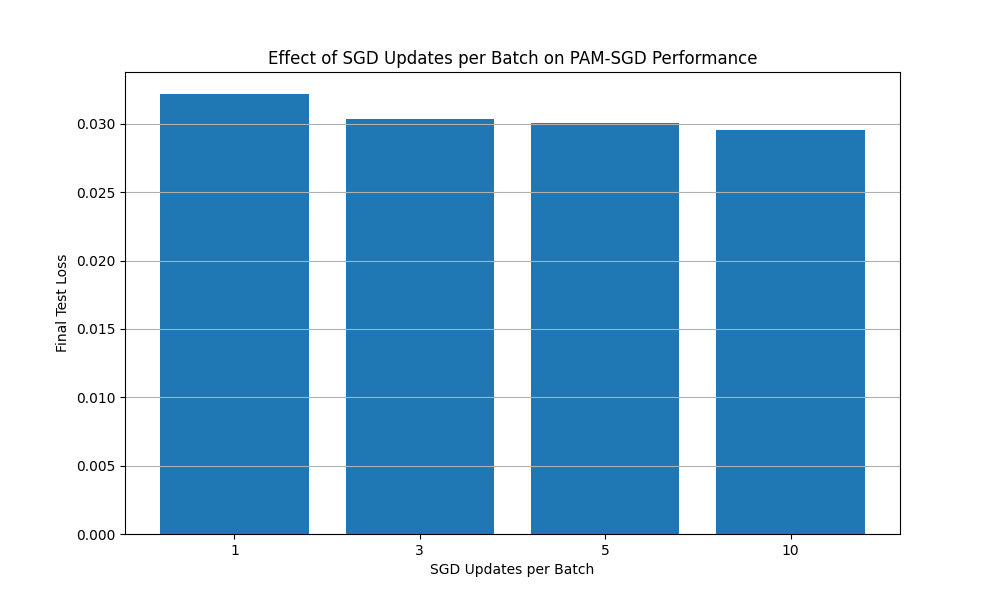
Figure 16: Effect of Multiple SGD Updates Per Batch on PAM-SGD Performance with ReLU. Test loss decreases with more updates per batch.

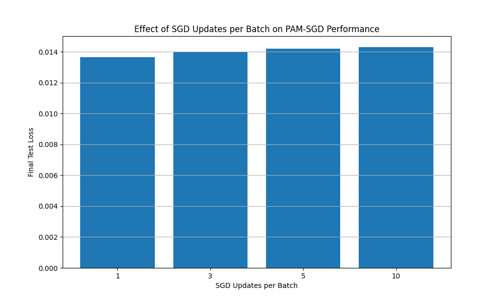
Figure 17: Effect of Multiple SGD Updates Per Batch on PAM-SGD Performance with TopK $K=15$. Test loss increases with more updates per batch, suggesting simpler optimization (single updates) maintains better balance.

E.2.4 TopK and ReLU activation patterns

Figure 18: Sparse activation patterns for ReLU activations. Plots showing which latent neurons activate for 5 different input digits, comparing SGD (left) and PAM-SGD (right) models. PAM-SGD activations are roughly five times denser.

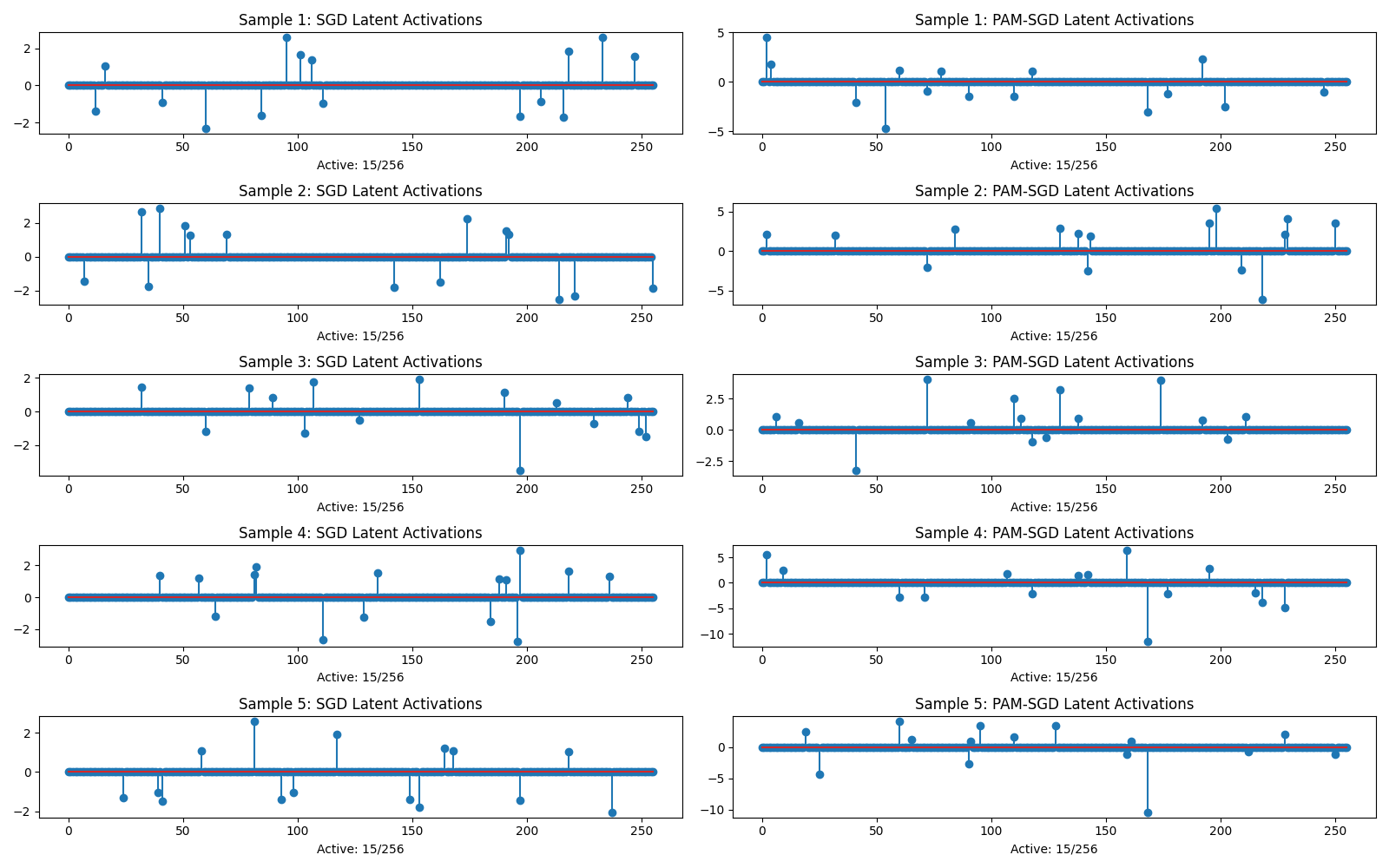
Figure 19: Sparse activation patterns for TopK $K=15$ activations. Plots showing which latent neurons activate for 5 different input digits, comparing SGD (left) and PAM-SGD (right) models. Each sample activates exactly $K=15$ neurons from the 256-dimensional latent space.

E.2.5 Ablation study adding weight decay

Small amounts of weight decay make SGD compete with PAM-SGD in the ReLU setting. (Figures˜20 and 21)

We experimented with adding weight decay in the 100% data setting. In the ReLU setting, we found that small amounts aided SGD performance to be competitive with PAM-SGD and had little effect on PAM-SGD. Increasing weight decay further however degraded both performances, especially PAM-SGD’s. In the TopK setting, weight decay just steadily degraded both performances.

Figure 20: Impact of weight decay on final test loss in the ReLU case.

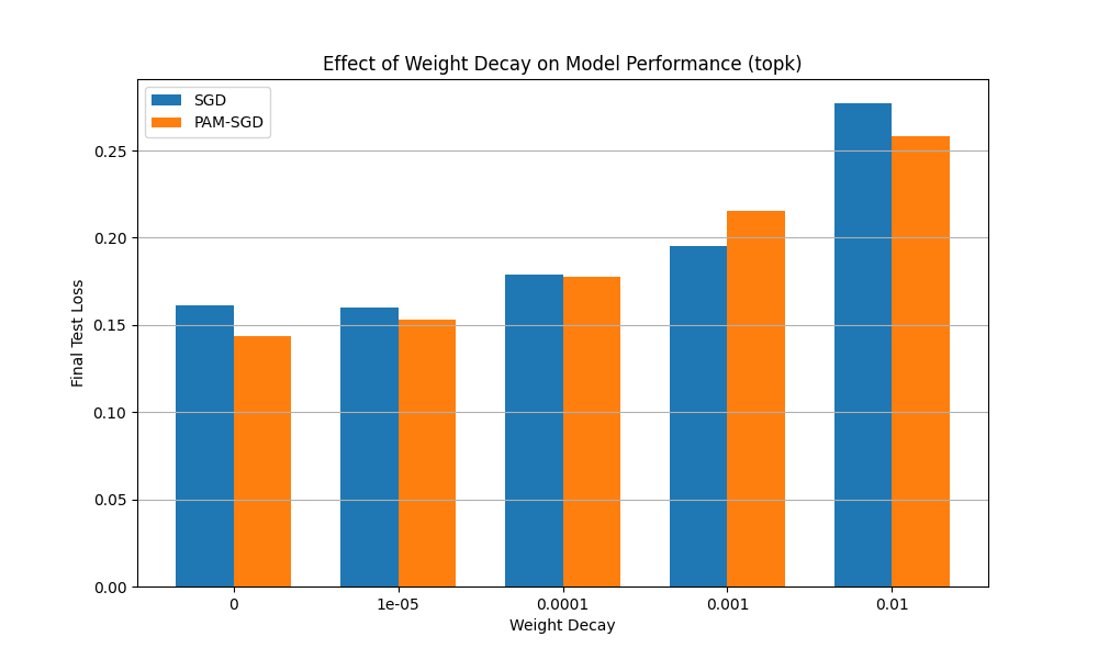
Figure 21: Impact of weight decay on final test loss in the TopK $K=15$ case.

E.2.6 Ablation study varying $\mu$ and $\nu$

Sensitivity to quadratic costs to move $\mu$ and $\nu$. (Figures˜22 and 23)

We studied the effect of varying the values of the parameters $\mu_{\text{enc}},\mu_{\text{dec}},\nu_{\text{enc}},$ and $\nu_{\text{dec}}$ from Equation˜3.1, in the 100% data setting. For ReLU activation, very small values for these parameters improve the test loss almost to zero for both SGD (where similar parameters can easily be introduced) and PAM-SGD. Further increases however degrade performance for both, rapidly in the case of PAM-SGD. For TopK increasing these parameters steadily degrades performance in both cases, though this may simply be due to these parameters slowing convergence and therefore worsening performance at the 50 epoch cut-off.

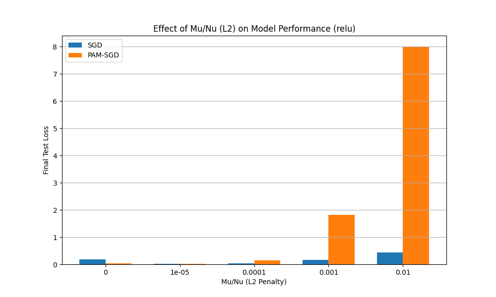
Figure 22: Effect of modifying the cost-to-move parameters on final test loss in the ReLU case.

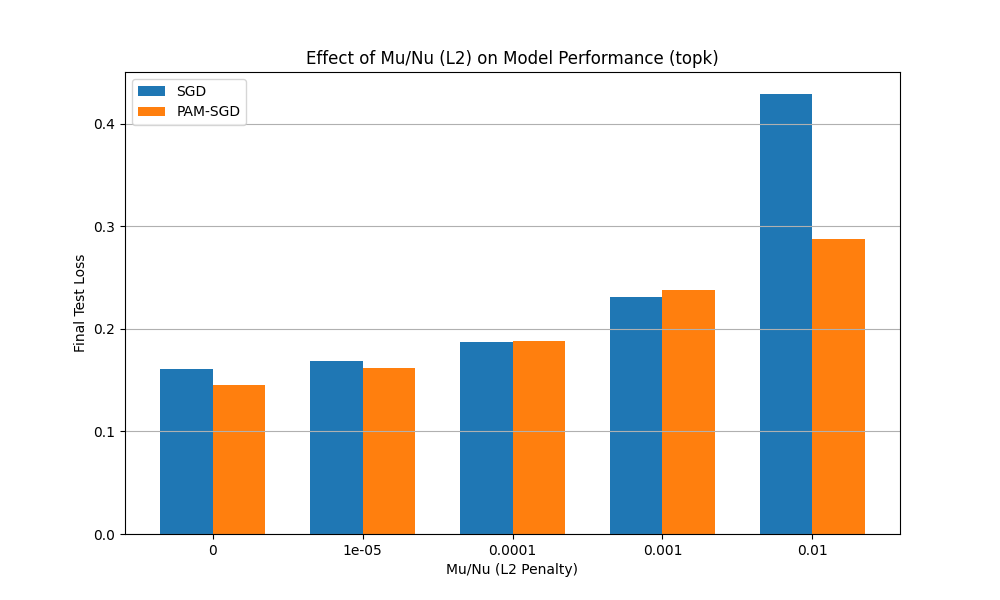
Figure 23: Effect of modifying the cost-to-move parameters on final test loss in the TopK $K=15$ case.

E.3 LLM Activation Experiments (Gemma–2-2B)

E.3.1 Additional ReLU test runs

PAM-SGD consistently outperforms SGD. (Figure˜24)

Owing to the stochasticity of the training algorithms, different results are obtained in every re-run of the training. However, the pattern of PAM-SGD outperforming SGD remained consistent.

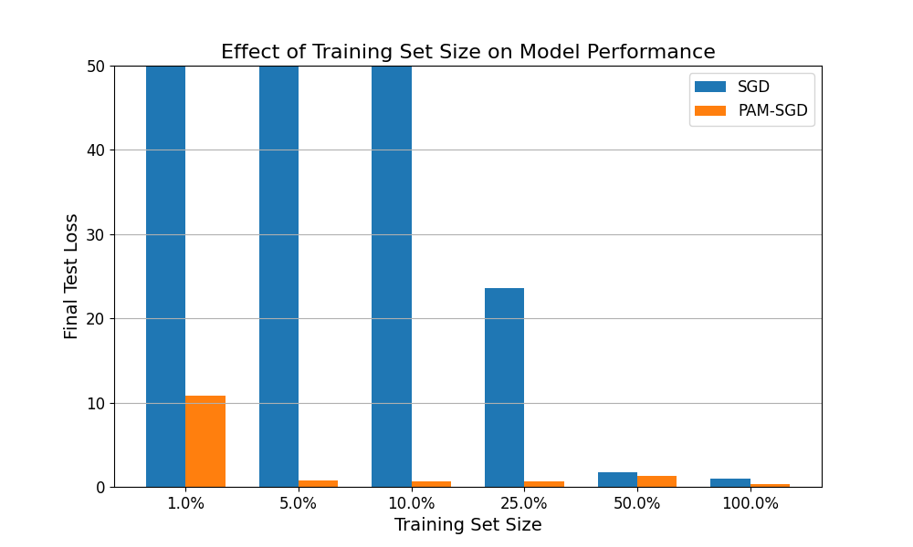
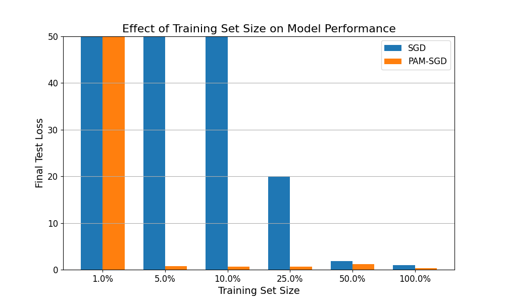
Figure 24: Final test loss across training set sizes for Gemma-2-2B, with ReLU activation, for two additional training runs. PAM-SGD retains an advantage at low data, and remains superior throughout, in both runs.

E.3.2 TopK activation experiments

Stability only at high sparsity and underperforms SGD. (Figures˜25, 26, 29, 28 and 27)

PAM-SGD was highly unstable for low values of $K$, with the test loss diverging rapidly. Only for larger values was the test loss stable, but fairly stagnant agross epochs even for very large $K$ (over 30% of the hidden dimension) leading us to choose $K=320$ as our default TopK sparsity. We speculate that this is because the LLM reconstruction is sufficiently complicated as to make being able to capture it with small $K$ unrealistic.

We furthermore compared SGD and PAM-SGD at various training data sizes for $K=320$ and $K=640$. We found that PAM-SGD consistently underperformed SGD in both cases, with the difference the smallest at low data sizes and again at high data sizes, with a surprising big rise in test loss for medium data sizes (with a maximum around 45%). This peak was consistent across multiple runs, so we suspect it is some fundamental issue perhaps caused by numerical instability. Inspecting the loss curves in the two cases shows that PAM-SGD only has well-behaved training and test loss in the low data regime, or at 100% data in the $K=640$ case.

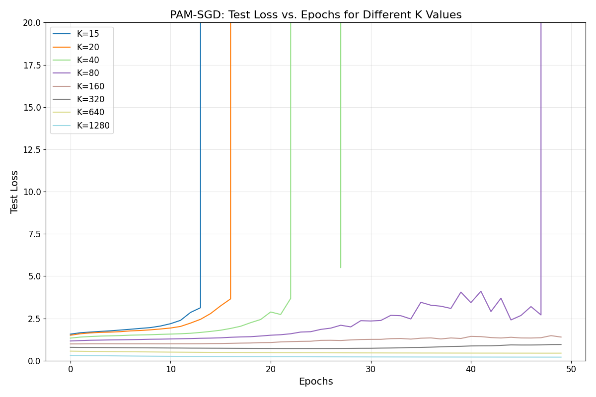
Figure 25: PAM-SGD test loss stable only for high values of $K$.

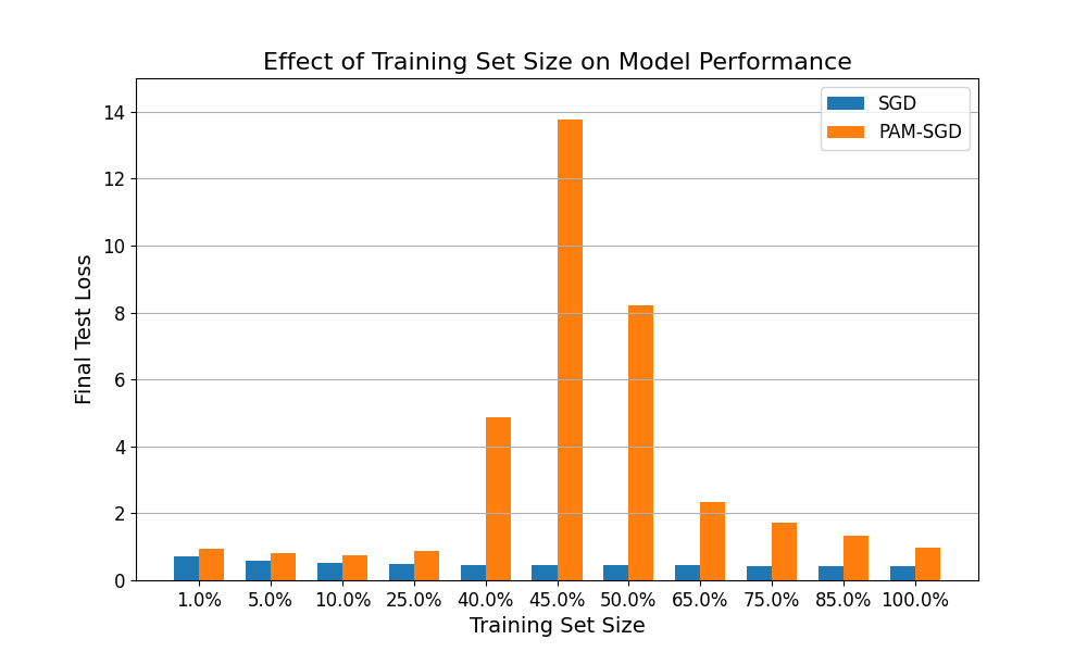
Figure 26: Final test loss across training set sizes for Gemma-2-2b with TopK activation, for $K=320$. PAM-SGD here consistently underperforms SGD, with a major peak at 45% data.

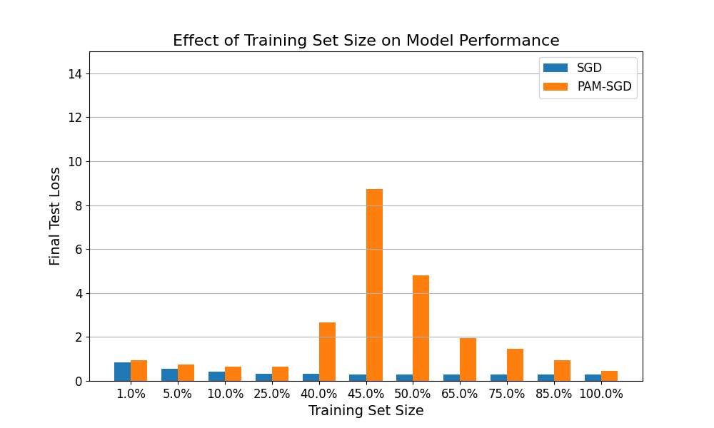
Figure 27: Final test loss across training set sizes for Gemma-2-2b with TopK activation, for $K=640$. PAM-SGD here consistently underperforms SGD, with a major peak at 45% data.

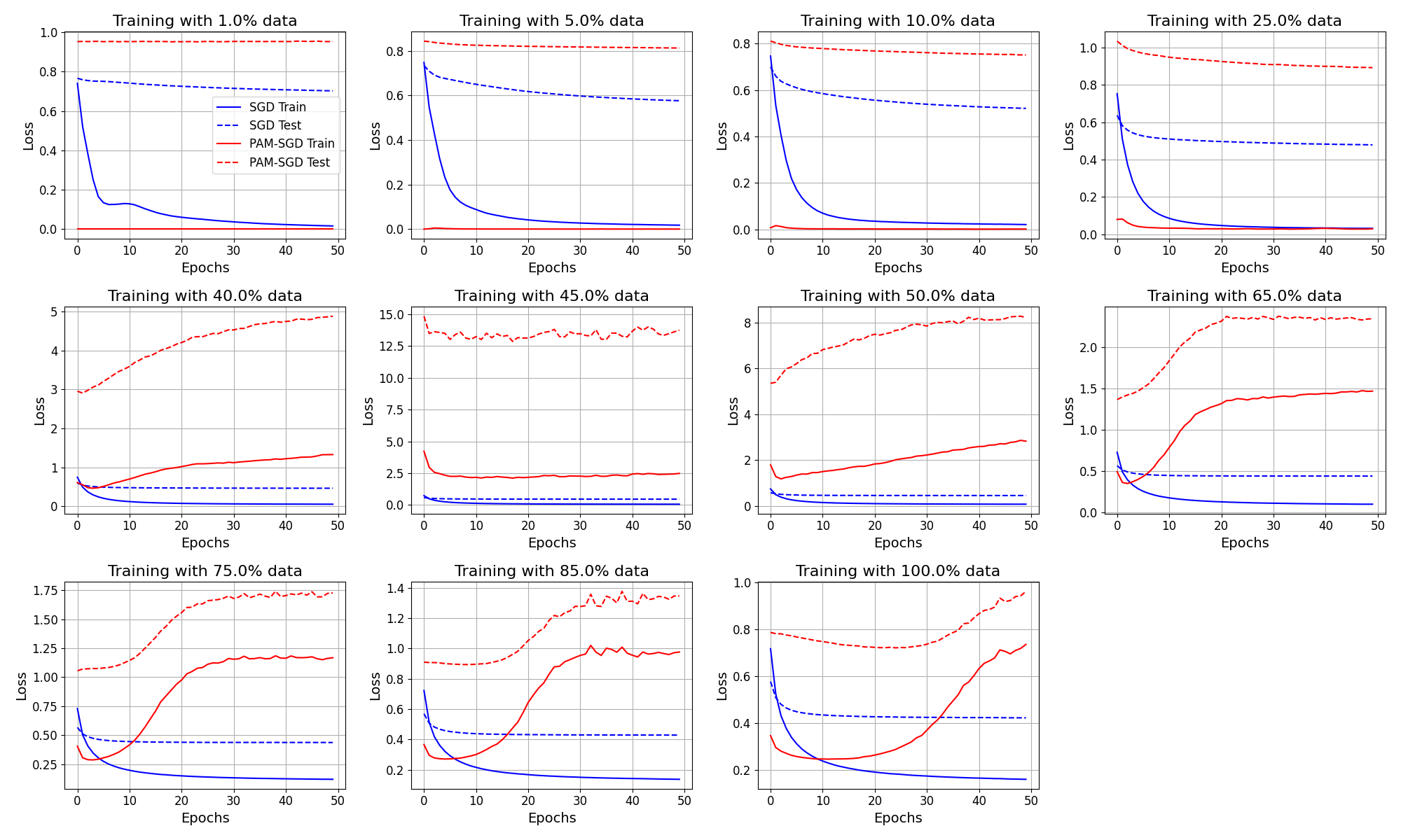
Figure 28: Training and test loss curves across training set sizes for Gemma-2-2b with TopK activation, for $K=320$. PAM-SGD has well-behaved training and test loss only for low data.

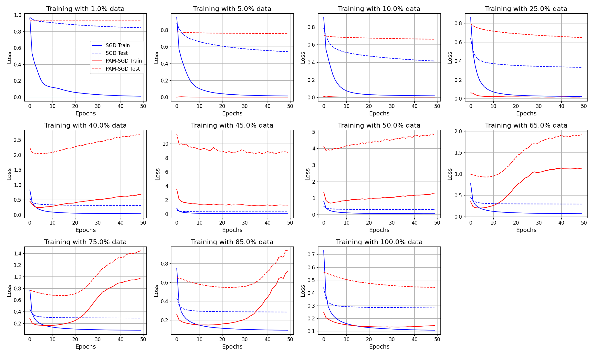
Figure 29: Training and test loss curves across training set sizes for Gemma-2-2b with TopK activation, for $K=640$. PAM-SGD has well-behaved training and test loss only for low data and 100% data.

E.3.3 TopK and ReLU activation patterns

Sparsity Comparison. (Figures˜30, 31 and 32)

TopK by design produces a constant sparsity $K=320$ for both SGD and PAM-SGD. ReLU produces much denser activations, around 58.5% (approx. 2400) for SGD and 49.6% (approx. 2000) for PAM-SGD. This increased sparsity from PAM-SGD is an important advantage of the method.

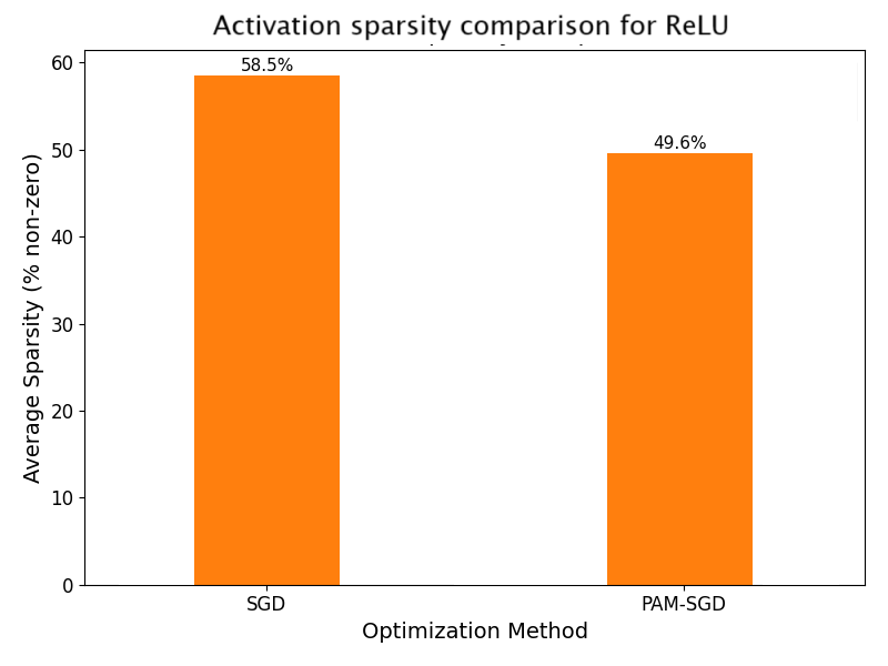
Figure 30: Activation sparsity comparison. ReLU yields much denser activations than TopK, and PAM-SGD activations about 15% sparser than SGD activations.

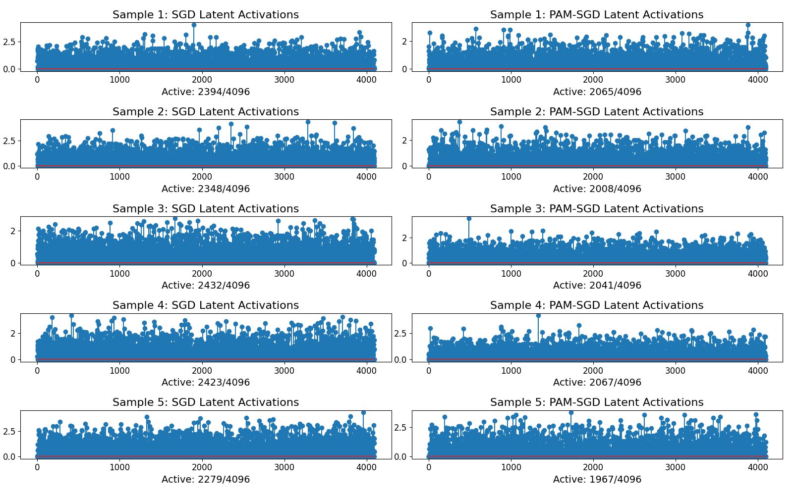
Figure 31: Sparse activation patterns. Plots showing which latent neurons were active in the ReLU case, comparing SGD (left) and PAM-SGD (right).

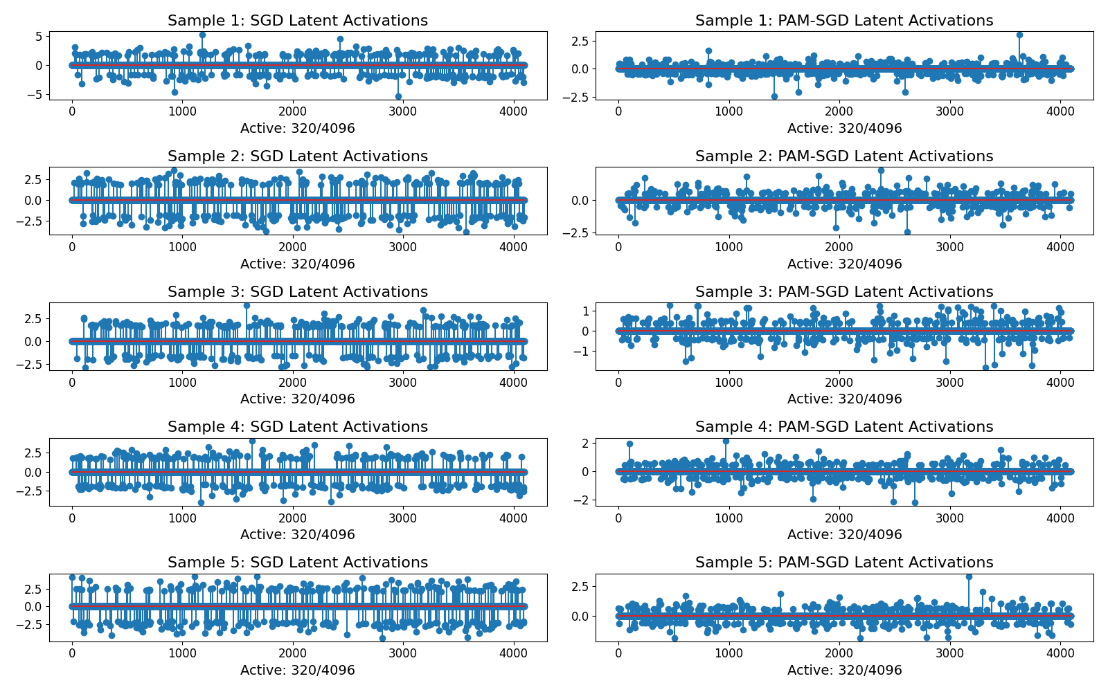
Figure 32: Sparse activation patterns. Plots showing which latent neurons were active in the TopK ($K=320$) case, comparing SGD (left) and PAM-SGD (right).

E.3.4 Ablation study varying SGD updates per batch in PAM-SGD

Number of SGD steps per batch matters for PAM-SGD. (Figures˜33 and 34)

For both the ReLU and TopK activations (with $K=320$), performance improves slightly when increasing SGD updates per batch from 1 to 3, but degrades beyond that. Too few updates prevent convergence of the inner optimization loop. Too many updates may lead to overfitting within the inner loop or instability due to misaligned gradients. PAM-SGD benefits from a moderate number of decoder updates per batch. An optimal value provides enough adaptation without overfitting, highlighting the importance of tuning this hyperparameter for practical deployments.

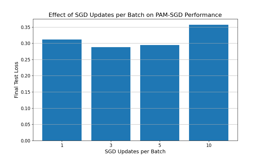
Figure 33: Effect of SGD Updates per Batch on PAM-SGD Test Loss with ReLU activation. Performance improves up to 3 updates but degrades beyond that, suggesting an optimal trade-off.

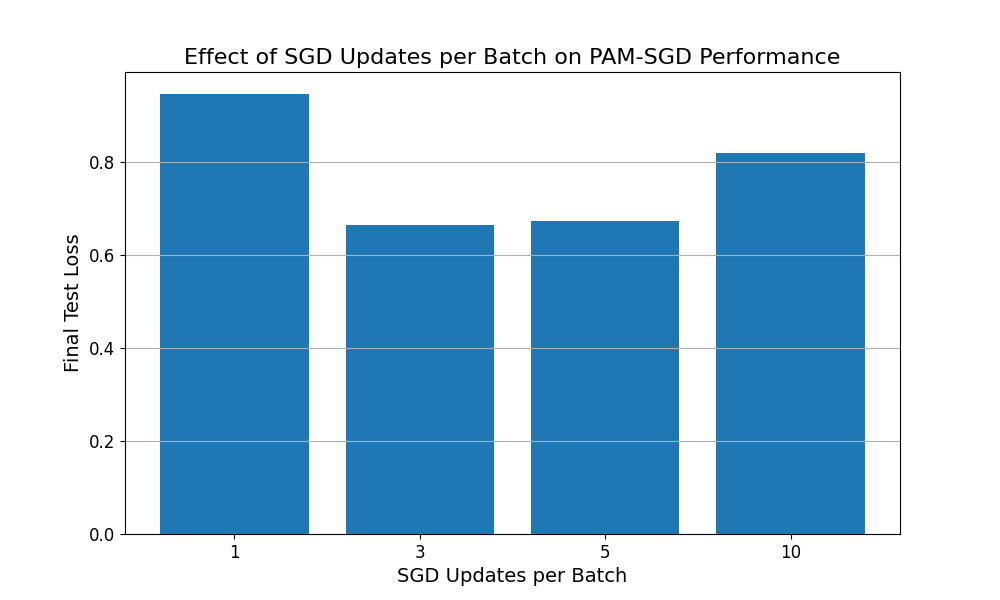
Figure 34: Effect of SGD Updates per Batch on PAM-SGD Test Loss with TopK activation. Performance again improves up to 3 updates but degrades beyond that.

E.3.5 Ablation study adding weight decay

Weight decay had a minor effect on performance. (Figures˜35 and 36)

Weight decay had a very minor effect on the SAE performance using either ReLU or TopK activations, with final test loss relatively constant, and PAM-SGD slightly outperforming SGD in the ReLU case and underperforming SGD in the TopK case. However, in the TopK case large values of weight decay are intially divergent before converging, whilst in the ReLU case this behaviour is less pronounced.

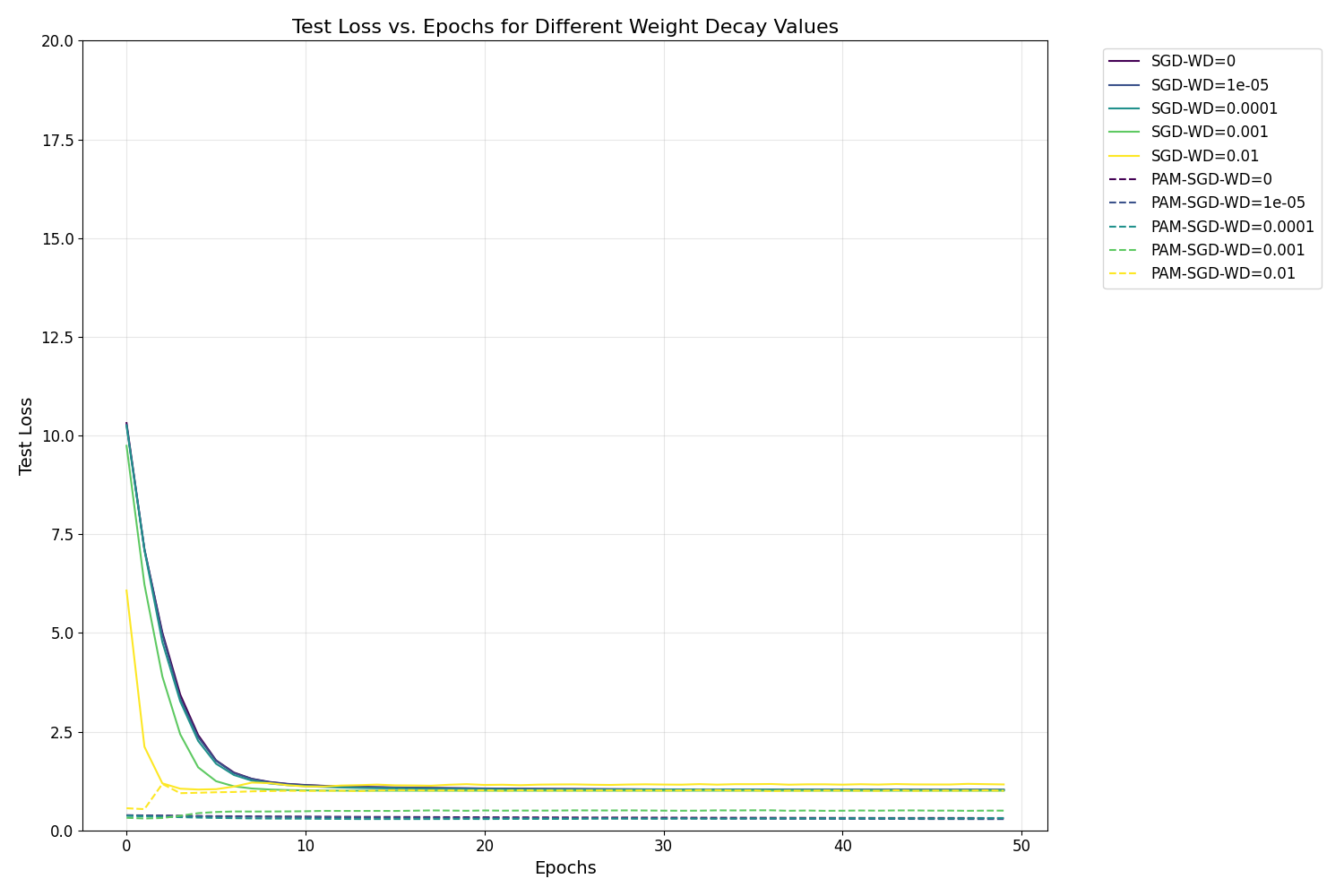
Figure 35: Training and test loss curves with various weight decay parameters, with ReLU activation.

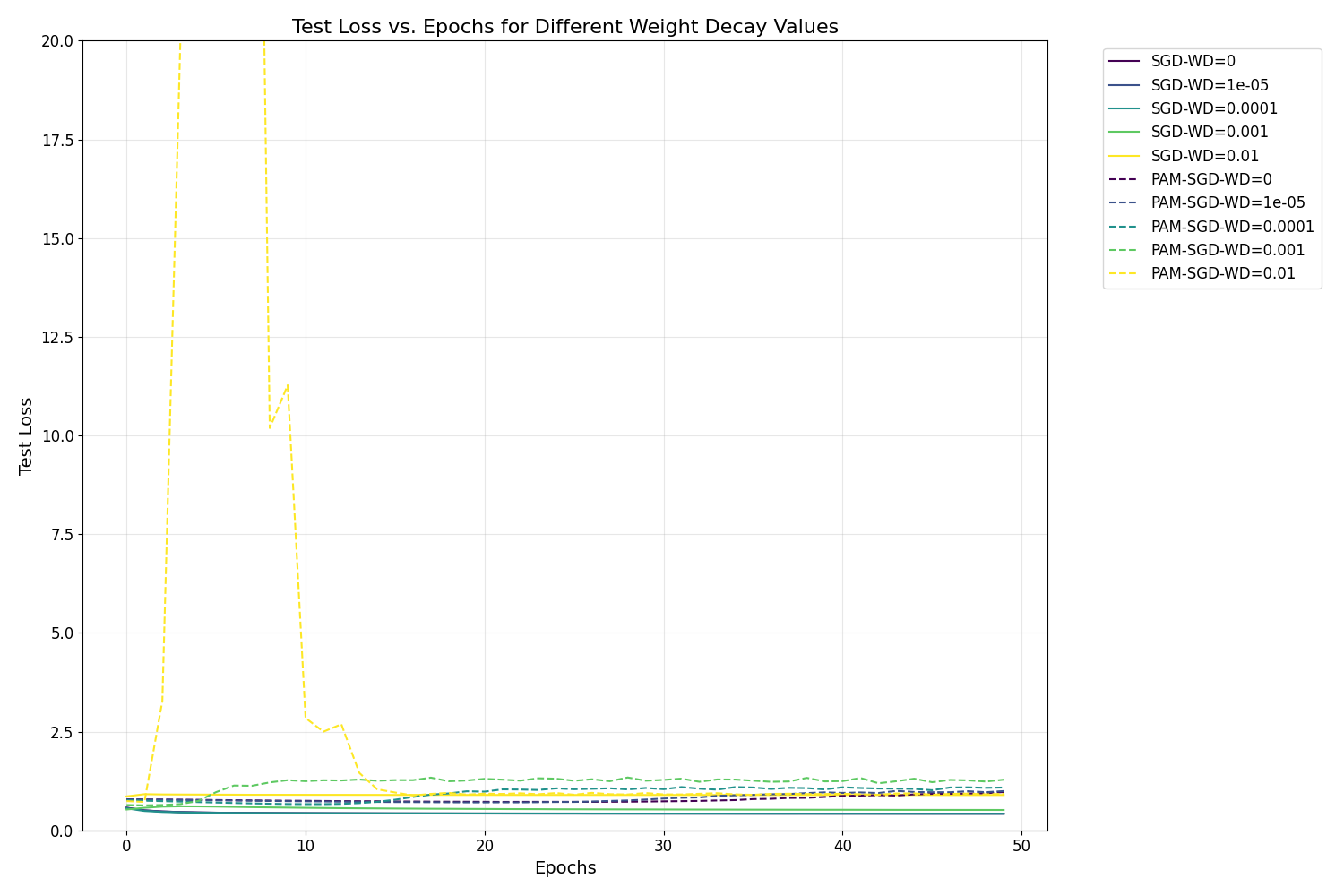
Figure 36: Training and test loss curves with various weight decay parameters, with TopK $K=320$ activation.

E.3.6 Ablation study varying the quadratic costs to move $\mu$ and $\nu$

Sensitivity to quadratic costs to move $\mu$ and $\nu$. (Figure˜37)

We studied the effect of varying the values of the parameters $\mu_{\text{enc}},\mu_{\text{dec}},\nu_{\text{enc}},$ and $\nu_{\text{dec}}$ from Equation˜3.1. For ReLU activation, we found that very small values of these parameters caused the test loss to begin diverging, perhaps due to numerical instability. Slightly larger values improved performance, but increases beyond that slowed the learning process to no clear gain. In the TopK case, this divergence occurred at larger values than for ReLU, but went away once the parameters were sufficiently large.

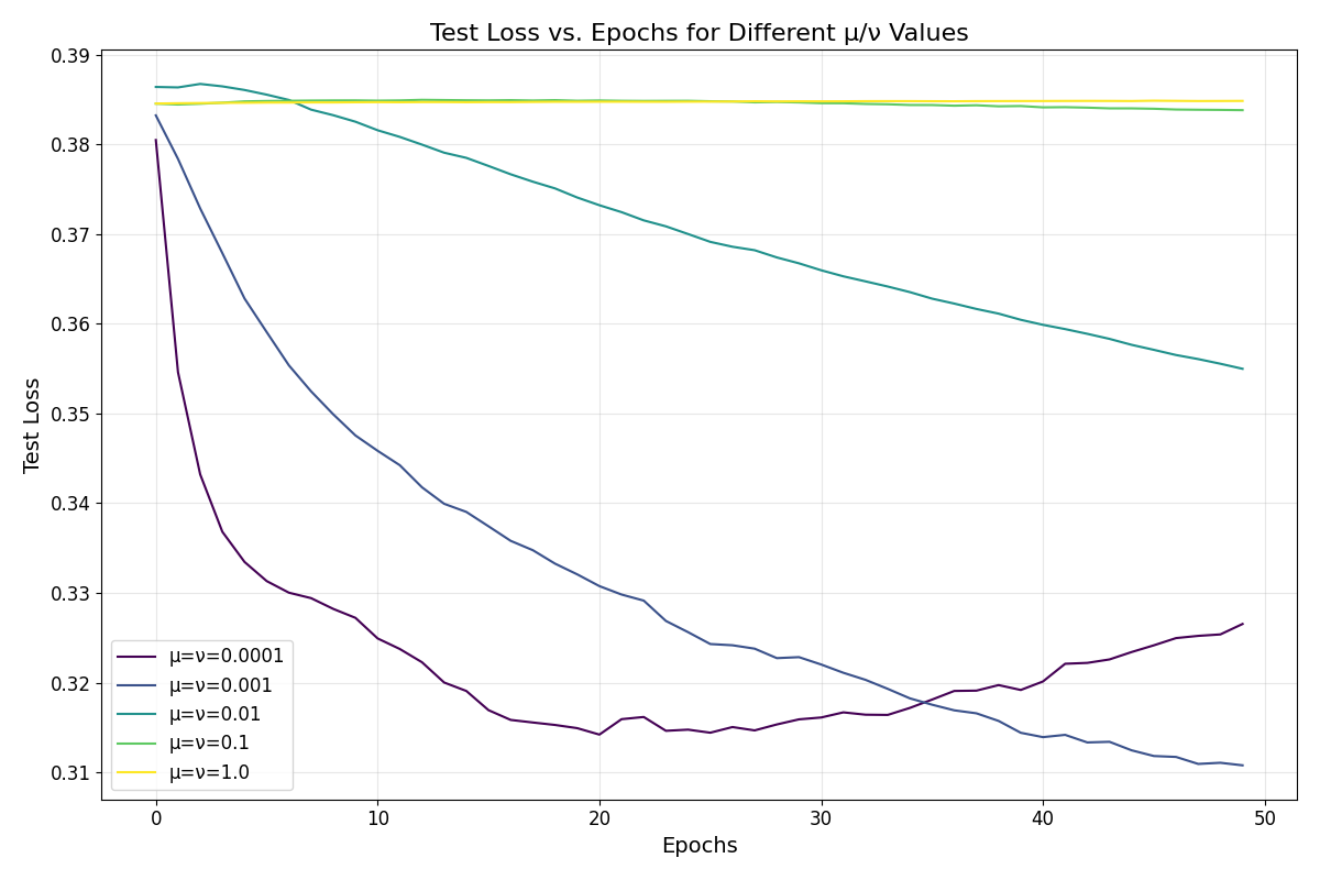
Figure 37: Loss curves for ReLU activation at different “cost to move” parameters.

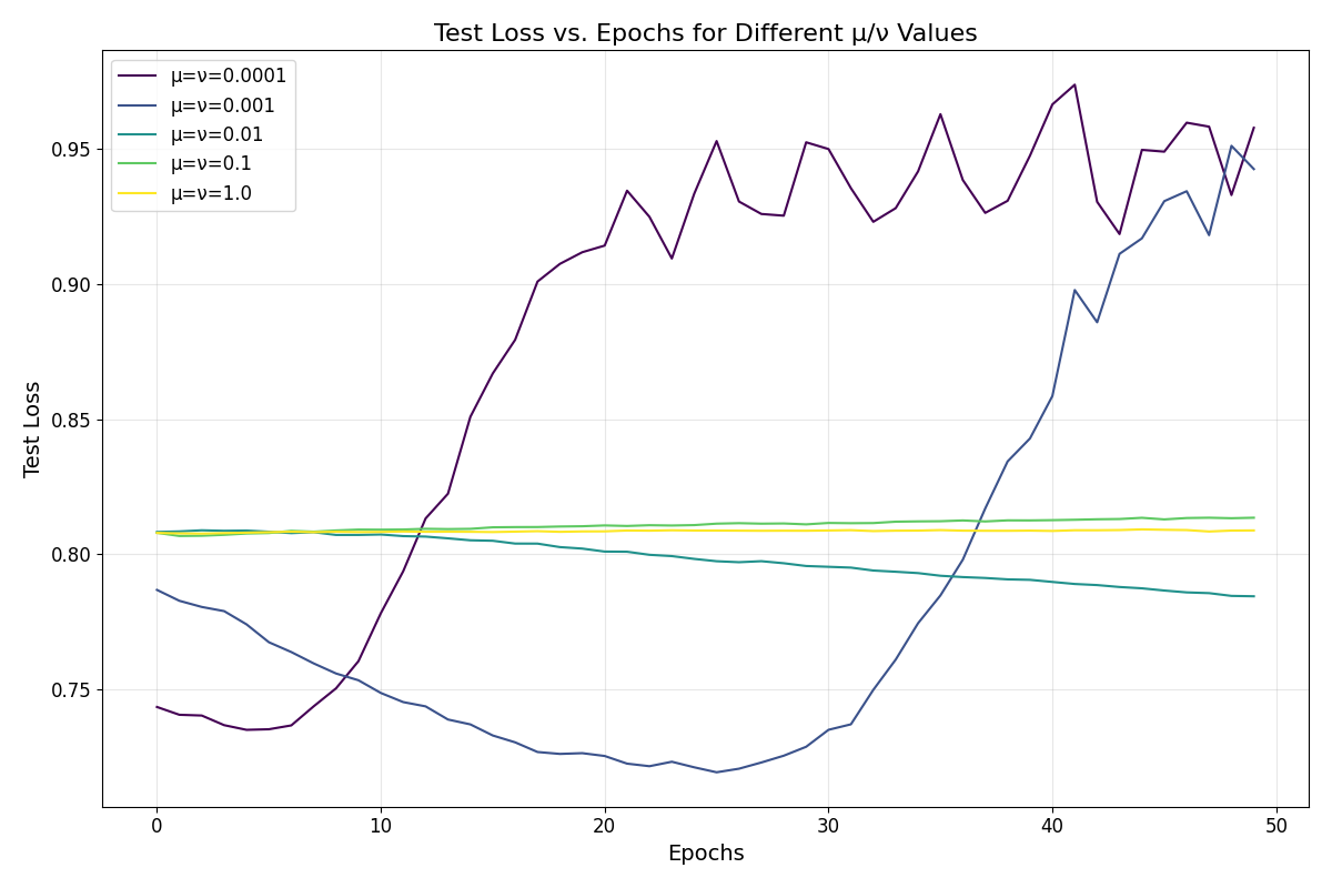
Figure 38: Loss curves for TopK activation ($K=320$) at different “cost to move” parameters.

References

- Ash & Bolker (1986) Ash, P. F. and Bolker, E. D. Generalized Dirichlet tessellations. Geometriae Dedicata, 20(2):209–243, Apr 1986. ISSN 1572-9168. doi: 10.1007/BF00164401. URL https://doi.org/10.1007/BF00164401.
- Attouch et al. (2010) Attouch, H., Bolte, J., Redont, P., and Soubeyran, A. Proximal alternating minimization and projection methods for nonconvex problems: An approach based on the Kurdyka-Łojasiewicz inequality. Mathematics of operations research, 35(2):438–457, 2010.
- Balestriero & Baraniuk (2018) Balestriero, R. and Baraniuk, R. A spline theory of deep learning. In Dy, J. and Krause, A. (eds.), Proceedings of the 35th International Conference on Machine Learning, volume 80 of Proceedings of Machine Learning Research, pp. 374–383. PMLR, 10–15 Jul 2018. URL https://proceedings.mlr.press/v80/balestriero18b.html.
- Bennett et al. (2009) Bennett, C., Miller, M., and Wolford, G. Neural correlates of interspecies perspective taking in the post-mortem atlantic salmon: an argument for multiple comparisons correction. NeuroImage, 47:S125, 2009. ISSN 1053-8119. doi: https://doi.org/10.1016/S1053-8119(09)71202-9. URL https://www.sciencedirect.com/science/article/pii/S1053811909712029. Organization for Human Brain Mapping 2009 Annual Meeting.
- Bolte et al. (2007) Bolte, J., Daniilidis, A., and Lewis, A. The Łojasiewicz Inequality for Nonsmooth Subanalytic Functions with Applications to Subgradient Dynamical Systems. SIAM Journal on Optimization, 17(4):1205–1223, 2007. doi: 10.1137/050644641.
- Bricken et al. (2023) Bricken, T., Templeton, A., Batson, J., Chen, B., Jermyn, A., Conerly, T., Turner, N., Anil, C., Denison, C., Askell, A., Lasenby, R., Wu, Y., Kravec, S., Schiefer, N., Maxwell, T., Joseph, N., Hatfield-Dodds, Z., Tamkin, A., Nguyen, K., McLean, B., Burke, J. E., Hume, T., Carter, S., Henighan, T., and Olah, C. Towards monosemanticity: Decomposing language models with dictionary learning. Transformer Circuits Thread, 2023. https://transformer-circuits.pub/2023/monosemantic-features/index.html.
- Elhage et al. (2022) Elhage, N., Hume, T., Olsson, C., Schiefer, N., Henighan, T., Kravec, S., Hatfield-Dodds, Z., Lasenby, R., Drain, D., Chen, C., et al. Toy models of superposition. arXiv preprint arXiv:2209.10652, 2022.
- Gao et al. (2025) Gao, L., la Tour, T. D., Tillman, H., Goh, G., Troll, R., Radford, A., Sutskever, I., Leike, J., and Wu, J. Scaling and evaluating sparse autoencoders. In The Thirteenth International Conference on Learning Representations, 2025. URL https://openreview.net/forum?id=tcsZt9ZNKD.
- Heap et al. (2025) Heap, T., Lawson, T., Farnik, L., and Aitchison, L. Sparse autoencoders can interpret randomly initialized transformers, 2025. URL https://arxiv.org/abs/2501.17727.
- Hindupur et al. (2025) Hindupur, S. S. R., Lubana, E. S., Fel, T., and Ba, D. Projecting assumptions: The duality between sparse autoencoders and concept geometry, 2025. URL https://arxiv.org/abs/2503.01822.
- Huben et al. (2024) Huben, R., Cunningham, H., Smith, L. R., Ewart, A., and Sharkey, L. Sparse autoencoders find highly interpretable features in language models. In The Twelfth International Conference on Learning Representations, 2024. URL https://openreview.net/forum?id=F76bwRSLeK.
- Humayun et al. (2024) Humayun, A. I., Balestriero, R., and Baraniuk, R. Deep networks always grok and here is why. In High-dimensional Learning Dynamics 2024: The Emergence of Structure and Reasoning, 2024. URL https://openreview.net/forum?id=NpufNsg1FP.
- Leask et al. (2025) Leask, P., Bussmann, B., Pearce, M., Bloom, J., Tigges, C., Moubayed, N. A., Sharkey, L., and Nanda, N. Sparse autoencoders do not find canonical units of analysis, 2025. URL https://arxiv.org/abs/2502.04878.
- Li & Pong (2017) Li, G. and Pong, T. K. Calculus of the Exponent of Kurdyka–Łojasiewicz Inequality and Its Applications to Linear Convergence of First-Order Methods. Foundations of Computational Mathematics, 18(5):1199–1232, aug 2017. doi: 10.1007/s10208-017-9366-8.
- Łojasiewicz (1964) Łojasiewicz, S. Triangulation of semi-analytic sets. Annali della Scuola Normale Superiore di Pisa-Classe di Scienze, 18(4):449–474, 1964.
- Makhzani & Frey (2014) Makhzani, A. and Frey, B. k-sparse autoencoders, 2014. URL https://arxiv.org/abs/1312.5663.
- Ng (2011) Ng, A. Sparse autoencoder. CS294A Lecture notes, 72(2011):1–19, 2011.
- Olah et al. (2017) Olah, C., Mordvintsev, A., and Schubert, L. Feature visualization. Distill, 2(11):e7, 2017.
- Olshausen & Field (1996) Olshausen, B. A. and Field, D. J. Emergence of simple-cell receptive field properties by learning a sparse code for natural images. Nature, 381(6583):607–609, 1996.
- Power et al. (2022) Power, A., Burda, Y., Edwards, H., Babuschkin, I., and Misra, V. Grokking: Generalization beyond overfitting on small algorithmic datasets, 2022. URL https://arxiv.org/abs/2201.02177.
- Rajamanoharan et al. (2024) Rajamanoharan, S., Lieberum, T., Sonnerat, N., Conmy, A., Varma, V., Kramár, J., and Nanda, N. Jumping ahead: Improving reconstruction fidelity with JumpReLU sparse autoencoders, 2024. URL https://arxiv.org/abs/2407.14435.
- Smith et al. (2025) Smith, L., Rajamanoharan, S., Conmy, A., McDougall, C., Kramar, J., Lieberum, T., Shah, R., and Nanda, N. Negative Results for SAEs On Downstream Tasks and Deprioritising SAE Research (GDM Mech Interp Team Progress Update #2), Mar 2025. URL https://www.alignmentforum.org/posts/4uXCAJNuPKtKBsi28/sae-progress-update-2-draft.
- Steinhaus (1957) Steinhaus, H. Sur la division des corps matériels en parties. Bull. Acad. Pol. Sci., Cl. III, 4:801–804, 1957. ISSN 0001-4095.
- Templeton et al. (2024) Templeton, A., Conerly, T., Marcus, J., Lindsey, J., Bricken, T., Chen, B., Pearce, A., Citro, C., Ameisen, E., Jones, A., Cunningham, H., Turner, N. L., McDougall, C., MacDiarmid, M., Freeman, C. D., Sumers, T. R., Rees, E., Batson, J., Jermyn, A., Carter, S., Olah, C., and Henighan, T. Scaling monosemanticity: Extracting interpretable features from Claude 3 Sonnet. Transformer Circuits Thread, 2024. URL https://transformer-circuits.pub/2024/scaling-monosemanticity/index.html.