Theoretical framework for designing phase change material systems

Abstract

Phase change materials (PCMs) hold considerable promise for thermal energy storage applications. However, designing a PCM system to meet specific performance presents a formidable challenge, given the intricate influence of multiple factors on the performance. To address this challenge, we hereby develop a theoretical framework that elucidates the melting process of PCMs. By integrating stability analysis with theoretical modeling, we derive a transition criterion to demarcate different melting regimes, and subsequently formulate the melting curve that uniquely characterizes the performance of an exemplary PCM system. This theoretical melting curve captures the key trends observed in experimental and numerical data across a broad parameter space, establishing a convenient and quantitative relationship between design parameters and system performance. Furthermore, we demonstrate the versatility of the theoretical framework across diverse configurations. Overall, our findings deepen the understanding of thermo-hydrodynamics in melting PCMs, thereby facilitating the evaluation, design, and enhancement of PCM systems.

1 Introduction

Due to their high energy storage density, nearly constant melting temperature, and zero-carbon emissions, solid-liquid phase change materials (PCMs) have increasingly been utilized across various domains, including cold chain logistics (Tong et al., 2021; Zhou et al., 2023), thermal comfort in buildings (Kishore et al., 2023; Ragoowansi et al., 2023), thermal energy storage (Gerkman & Han, 2020; Zhang et al., 2023), and electronic thermal management (Wang et al., 2022a; Liu et al., 2022). The performance of a PCM system is primarily governed by its energy storage capacity and power density (Gur et al., 2012; Woods et al., 2021; Yang et al., 2021; Fu et al., 2022; Chen et al., 2022), which are influenced by various design parameters embedded in material properties, system geometries, and operational conditions (Woods et al., 2021; Yang et al., 2021). Consequently, achieving the desired performance under specific conditions necessitates meticulous selection of storage materials and thoughtful design of system geometries. However, universal guidelines for this practice are not yet established  (Gao & Lu, 2021; Yang et al., 2021; Wang et al., 2022b; He et al., 2022), calling for deeper insights into the physical principles governing how design parameters impact system performance.

The performance indicators—energy storage capacity and power density—are determined by the maximum melted amount and melting rate of PCMs, respectively. Thus, the performance can be exclusively represented by the temporal evolution of PCM’s melted volume, which, in dimensionless form, is the evolution of liquid fraction (melting curve). Indicatively, the task of investigating the effects of design parameters on performance can be restated as identifying their impacts on the melting curve.

The melting curve has been typically recognised a composite of two segments, corresponding to successive regimes underwent by the storage process: initially dominated by conduction and then by convection (Ho & Viskanta, 1984; Gau & Viskanta, 1986; Wang et al., 1999; Duan et al., 2019; Li et al., 2022). Despite this understanding, a comprehensive model for the melting curve is lacking(Verma et al., 2008; Dutil et al., 2011), as current knowledge of the transitional scenario remains scarce (Azad et al., 2021a, b, 2022), commonly limited to empirical fits from experimental or numerical data (Wang et al., 1999; Vogel et al., 2016; Duan et al., 2019; Li & Su, 2023).

In this work, we delineate the transitional scenario of melting PCM and subsequently develop a theoretical framework to model the melting curve. The resulting model encapsulates the essential physics of PCM melting, concomitantly agreeing well with experimental and numerical data. The associated theoretical formula quantifies the impacts of material properties, geometric features, and operational conditions on system performance, providing convenient guiding principles for material selection and geometric design of PCM systems.

2 Storage performance of PCM system

2.1 Problem description

We illustrate the theoretical framework using a minimal yet representative enclosure of PCM (Dhaidan & Khodadadi, 2015)—a rectangular cavity of width $W$ and height $H$ (see figure 1a). It is filled with solid PCM initialized at the ambient temperature $\tilde{T}=T_{c}$, which is below the fusion (melting) temperature $T_{f}$. Keeping its top and bottom walls insulated, the cavity’s left wall absorbs heat from a hot working device at temperature $\tilde{T}=T_{h}>T_{f}$, with its right boundary subject to a cold ambient environment at $\tilde{T}=T_{c}<T_{f}$. This configuration finds typical application in enhancing thermal comfort in buildings (Lachheb et al., 2024), where PCM is encapsulated within bricks, with $T_{f}$ lying between indoor ($T_{c}$) and outdoor ($T_{h}$) temperatures. The ideal configuration—where $T_{f}$ always equals $T_{c}$, preventing any heat transfer in the solid phase—has been discussed in previous studies (Esfahani et al., 2018; Favier et al., 2019; Yang et al., 2022; Li et al., 2022).

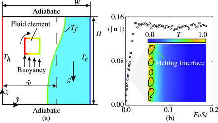
Figure 1: (a) A rectangular cavity filled with subcooled PCM, maintaining temperatures at $T_{h}$ (hot) and $T_{c}$ (cold) at the left and right boundaries, respectively. (b) Time evolution of the domain averaged velocity $\langle|\boldsymbol{u}|\rangle=(g\alpha\Delta T_{l}H)^{-1/2}\int|\boldsymbol{\tilde{u}}|{\rm d}{\mathcal{V}}/\mathcal{V}_{0}$, where $\mathcal{V}_{0}=WH$. Here, ${\textit{Ra}}=10^{7}$, ${\textit{Pr}}=0.1$, ${\textit{St}}=0.1$, ${\textit{S}}_{T}=1.0$, and $\gamma=1.0$. The inset shows the instantaneous temperature field and streamlines at ${\textit{Fo}}{\textit{St}}=0.0046$.

Using tildes to indicate dimensional variables, the thermo-hydrodynamic equations for the liquid phase read

$$\gradient\cdot\boldsymbol{\tilde{u}} =0,$$ (1a)

$$\frac{\partial{\boldsymbol{\tilde{u}}}}{\partial\tilde{t}}+\boldsymbol{{\tilde{u}}}\cdot\gradient\boldsymbol{\tilde{u}} =\boldsymbol{g}\alpha({\tilde{T}}-T_{0})+{\nu\nabla^{2}\boldsymbol{{\tilde{u}}}}-\frac{\gradient{{\tilde{p}}}}{\rho_{0}},$$ (1b)

$$\frac{\partial{\tilde{T}}}{\partial\tilde{t}}+\boldsymbol{\tilde{u}}\cdot\gradient\tilde{T} ={\kappa\nabla^{2}\tilde{T}},$$ (1c)

where $\boldsymbol{\tilde{u}}$, $\tilde{T}$, and $\tilde{p}$ denote the velocity, temperature, and pressure of the liquid, respectively; its kinematic viscosity is $\nu$, while the thermal expansion coefficient and diffusivity are $\alpha$ and $\kappa$, respectively. Here, $\rho_{0}$ denotes the reference density measured at the reference temperature $T_{0}=(T_{h}+T_{f})/2$, and $\boldsymbol{g}$ indicates the gravitational acceleration. At the melting interface between the solid ($s$) and liquid ($l$) phase, the Stefan condition $\mathcal{L}\boldsymbol{\tilde{V}}/C_{p}=[(\kappa\gradient\tilde{T})_{s}-(\kappa\gradient\tilde{T})_{l}]\cdot\boldsymbol{n}$ holds, where $\mathcal{L}$ and $C_{p}$ are the specific latent heat and specific heat, respectively; $\boldsymbol{\tilde{V}}$ represents the velocity of the interface, and $\boldsymbol{n}$ denotes its liquid-facing unit normal.

The above governing equations denote that the material properties affecting the system performance include $\alpha$, $T_{f}$, $\nu$, $\kappa$, $C_{p}$, and $\mathcal{L}$. Their effects, along with those of the geometry ($W$ and $H$), and the working conditions ($T_{h}$ and $T_{c}$) are characterised by five dimensionless numbers: Rayleigh number Ra, Prandtl number Pr, Stefan number St, subcooling strength ${\textit{S}}_{T}$, and the cavity’s aspect ratio $\gamma$, defined as

$${\textit{Ra}}=\frac{g\alpha\Delta T_{l}H^{3}}{\nu\kappa},~{\textit{Pr}}=\frac{\nu}{\kappa},~\textit{St}=\frac{C_{p}\Delta T_{l}}{\mathcal{L}},{\textit{S}}_{T}=\frac{\Delta T_{s}}{\Delta T_{l}},~\gamma=\frac{W}{H}.$$ (2)

Here, $\Delta T_{s}=T_{f}-T_{c}$ and $\Delta T_{l}=T_{h}-T_{f}$ are the temperature differences across the solid and liquid phases, respectively. Additionally, the melting behavior of PCMs is characterized by the Nusselt number Nu, Fourier time Fo, and liquid fraction $f$,

$${\textit{Nu}}=-\frac{H}{\Delta T_{l}}\langle\frac{\partial\tilde{T}}{\partial\tilde{y}}\rangle_{\tilde{y}=0},~{\textit{Fo}}=\frac{\kappa\tilde{t}}{W^{2}},~f=\frac{\tilde{w}}{W},$$ (3)

where $\tilde{w}$ is the average thickness of the liquid layer (figure 1a), and $\langle~\rangle_{\tilde{y}=0}$ denotes spatial averaging along the hot wall at $\tilde{y}=0$.

2.2 Linear stability analysis

We obtain the transition criterion through linear stability analysis, choosing the endpoint of conduction-dominated regime as the base state. Since the horizontal temperature gradient imposes a heterogeneous buoyancy on the fluid (figure 1a), the corresponding base flow $\boldsymbol{\tilde{u}}_{b}$ is not stationary, as evidenced by the temporal evolution of the domain-averaged velocity $\langle|\boldsymbol{u}|\rangle$ in figure 1b. This non-stationary base flow $\boldsymbol{\tilde{u}}_{b}$ differs from the quiescent counterpart of the canonical Rayleigh-Bénard convection, and cannot be derived analytically. However, the base liquid temperature $\tilde{T}_{b}$ is readily calculable, because the convective heat transfer is negligible in the conduction-dominated regime. By solving the heat conduction equation, we obtain $\tilde{T}_{b}=T_{h}-{\Delta T_{l}}\tilde{y}/{\tilde{w}_{b}}$, where $\tilde{w}_{b}=W/(1+{\textit{S}}_{T}^{\ast})$ results from the energy balance between the liquid and solid phases, $\Delta T_{l}/\tilde{w}_{b}=\Delta T_{s}/\left(W-\tilde{w}_{b}\right)$. Here, the superscript ^∗ indicates that ${\textit{S}}_{T}^{\ast}$ is the critical subcooling strength required for the base state to reach the onset of instability.

To linearise (1), we decompose the flow and temperature fields into the base state $\left(\tilde{\boldsymbol{u}}_{b},\tilde{p}_{b},\tilde{T}_{b}\right)$ and the disturbance state $\left(\tilde{\boldsymbol{u}}^{\prime},\tilde{p}^{\prime},\tilde{T}^{\prime}\right)$, such that $\left(\tilde{\boldsymbol{u}},\tilde{p},\tilde{T}\right)=\left(\tilde{\boldsymbol{u}}_{b},\tilde{p}_{b},\tilde{T}_{b}\right)+\left(\tilde{\boldsymbol{u}}^{\prime},\tilde{p}^{\prime},\tilde{T}^{\prime}\right)$. Selecting $\tilde{w}_{b}$ as the length scale, $U_{0}$ and $U$ the base and perturbation velocity scales, respectively, we derive the dimensionless linearised equations for $\left(\tilde{\boldsymbol{u}}^{\prime},\tilde{p}^{\prime},\tilde{T}^{\prime}\right)$,

$$\gradient\cdot\boldsymbol{u}^{\prime} =0,$$ (4a)

$$\frac{\partial{\boldsymbol{u}^{\prime}}}{\partial t}+\frac{U_{0}\tilde{w}_{b}}{\kappa}(\boldsymbol{u}_{b}\cdot\gradient{\boldsymbol{u}^{\prime}}+\boldsymbol{u}^{\prime}\cdot\gradient{\boldsymbol{u}_{b}}) =\frac{{\textit{Ra}}{\textit{Pr}}\gamma^{3}}{(1+{\textit{S}}_{T}^{\ast})^{3}}T^{\prime}\boldsymbol{e_{x}}+{\textit{Pr}}{\nabla^{2}}\boldsymbol{u}^{\prime}-\gradient{{p^{\prime}}},$$ (4b)

$$\frac{\partial{T^{\prime}}}{\partial t}-v^{\prime}+\frac{U_{0}\tilde{w}_{b}}{\kappa}\boldsymbol{u}_{b}\cdot\gradient T^{\prime} ={\nabla^{2}}T^{\prime},$$ (4c)

where we have also chosen $\tilde{w}_{b}^{2}/\kappa$ as the characteristic time, $\rho_{0}\kappa U/\tilde{w}_{b}$ the characteristic pressure, and $\Delta T_{l}U\tilde{w}_{b}/\kappa$ the characteristic temperature. Here, $v^{\prime}$ denotes the $y$-component of the dimensionless perturbation velocity $\boldsymbol{u}^{\prime}$.

We note that $U_{0}\tilde{w}_{b}/\kappa$ in  (4b) and (4c) represents the Péclet number, which measures the relative strength of convection to conduction. Since this number is inherently small in the conduction-dominated base state, we simplify the theoretical analysis by neglecting all terms involving $U_{0}\tilde{w}_{b}/\kappa$ in  (4). This assumption proves reasonable, as will be verified a posterior by numerical simulations (see appendix B). With this simplification, we obtain

$$\gradient\cdot\boldsymbol{u}^{\prime} =0,$$ (5a)

$$\frac{\partial{\boldsymbol{u}^{\prime}}}{\partial t} =\frac{{\textit{Ra}}{\textit{Pr}}\gamma^{3}}{(1+{\textit{S}}_{T}^{\ast})^{3}}T^{\prime}\boldsymbol{e_{x}}+{\textit{Pr}}\nabla^{2}\boldsymbol{u}^{\prime}-\gradient{{p^{\prime}}},$$ (5b)

$$\frac{\partial{T^{\prime}}}{\partial t}-v^{\prime} =\nabla^{2}T^{\prime}.$$ (5c)

Using the normal mode approach, a dimensionless perturbation field $\phi$ of either velocity, temperature, or pressure is expressed as $\phi^{\prime}(x,y,t)=\hat{\phi}(y)\exp({\rm i}\mathcal{K}x+\sigma t)$, where $\hat{\phi}$ presents the complex magnitude of perturbation, $\mathcal{K}$ and $\sigma$ stand for the wavenumber and growth rate, respectively; here, ${\rm i}=\sqrt{-1}$. Substituting the normal modes into  (5), we obtain the governing equations for the perturbation magnitudes,

$$0 ={\rm i}\mathcal{K}\hat{u}+\frac{\partial\hat{v}}{\partial y},$$ (6a)

$$\sigma\hat{u} =\frac{{\textit{Ra}}{\textit{Pr}}\gamma^{3}}{(1+{{\textit{S}}_{T}^{\ast}})^{3}}\hat{T}+{\textit{Pr}}\left(\frac{\partial^{2}\hat{u}}{\partial y^{2}}-\mathcal{K}^{2}\hat{u}\right)-{\rm i}\mathcal{K}\hat{p},$$ (6b)

$$\sigma\hat{v} ={\textit{Pr}}\left(\frac{\partial^{2}\hat{v}}{\partial y^{2}}-\mathcal{K}^{2}\hat{v}\right)-\frac{\partial\hat{p}}{\partial y},$$ (6c)

$$\sigma\hat{T} =\left(\frac{\partial^{2}\hat{T}}{\partial y^{2}}-\mathcal{K}^{2}\hat{T}\right)+\hat{v}.$$ (6d)

The corresponding boundary conditions at the hot wall $y=0$ are

$$\hat{u}=\hat{v}=0,~\hat{T}=0.$$ (7)

Those at the melting interface $y=1$ read

$$\hat{u}=\hat{v}=0,~\mathcal{K}\hat{T}{\rm coth}(\mathcal{K}{{\textit{S}}_{T}^{\ast}})+\frac{\partial\hat{T}}{\partial y}=0,$$ (8)

where the condition for $\hat{T}$ is derived from the Stefan condition (Davis et al., 1984; Toppaladoddi & Wettlaufer, 2019; Lu et al., 2022).

Equations (6), (7), and (8) indicate that the transition depends on Pr, Ra, $\gamma$, and ${{\textit{S}}_{T}^{\ast}}$. To investigate the influence of these parameters, we simplify  (5) into a single equation representing the marginal state ($\sigma=0$). Taking the divergence of  (5b) and using (5a), we derive

$$0=\frac{{\textit{Ra}}{\textit{Pr}}\gamma^{3}}{(1+{\textit{S}}_{T}^{\ast})^{3}}\frac{\partial T^{\prime}}{\partial x}-{\nabla^{2}}{{p^{\prime}}}.$$ (9)

Next, differentiating  (9) with respect to $y$ results in

$$0=\frac{{\textit{Ra}}{\textit{Pr}}\gamma^{3}}{(1+{\textit{S}}_{T}^{\ast})^{3}}\frac{\partial^{2}T^{\prime}}{\partial x\partial y}-{\nabla^{2}}{\frac{\partial p^{\prime}}{\partial y}}.$$ (10)

We then take the Laplacian of the $y$-component of  (5b) and obtain

$$\frac{\partial}{\partial t}{\nabla^{2}}{v^{\prime}}={\textit{Pr}}{\nabla^{4}}v^{\prime}-{\nabla^{2}}\frac{\partial p^{\prime}}{\partial y}.$$ (11)

Further subtracting  (10) from  (11) yields:

$$\frac{\partial}{\partial t}{\nabla^{2}}{v^{\prime}}={\textit{Pr}}{\nabla^{4}}v^{\prime}-\frac{{\textit{Ra}}{\textit{Pr}}\gamma^{3}}{(1+{\textit{S}}_{T}^{\ast})^{3}}\frac{\partial^{2}T^{\prime}}{\partial x\partial y}.$$ (12)

Incorporating the normal modes into  (5c) and  (12), the perturbation magnitudes at the marginal state ($\sigma=0$) are governed by

$$\mathcal{K}^{2}\hat{T}-\hat{v}-\hat{T}^{(2)}=0,$$ (13a)

$$-{\rm i}\mathcal{K}\gamma^{3}{\textit{Ra}}\hat{T}^{(1)}+\mathcal{K}^{2}(1+{\textit{S}}_{T}^{\ast})^{3}(\mathcal{K}^{2}\hat{v}-2\hat{v}^{(2)})+(1+{\textit{S}}_{T}^{\ast})^{3}\hat{v}^{(4)}=0,$$ (13b)

where $\hat{T}^{(n)}=\frac{\partial^{n}\hat{T}}{\partial y^{n}}$ and $\hat{v}^{(n)}=\frac{\partial^{n}\hat{v}}{\partial y^{n}}$. By eliminating $\hat{v}$, we derive

$$\mathcal{K}^{6}\hat{T}-\frac{{\rm i}{\textit{Ra}}\gamma^{3}\mathcal{K}\hat{T}^{(1)}}{(1+{{\textit{S}}_{T}^{\ast}})^{3}}=3\mathcal{K}^{4}\hat{T}^{(2)}-3\mathcal{K}^{2}\hat{T}^{(4)}+\hat{T}^{(6)},$$ (14)

which suggests that the transition is characterized solely by a critical effective Rayleigh number ${\textit{Ra}}_{e}^{\ast}={\textit{Ra}}\gamma^{3}/(1+{{\textit{S}}_{T}^{\ast}})^{3}$.

2.3 Results and discussions

Realizing the critical liquid fraction $f^{\ast}=1/\left(1+{\textit{S}}_{T}^{\ast}\right)$ upon substituting $\tilde{w}_{b}=W/(1+{\textit{S}}_{T}^{\ast})$ into  (3), we further obtain

$$f^{\ast}=\left(\frac{{\textit{Ra}}_{e}^{\ast}}{{\textit{Ra}}\gamma^{3}}\right)^{1/3}.$$ (15)

Applying a spectral method (Weideman & Reddy, 2000) to (6)–(8), we calculate $f^{\ast}=1/\left(1+{\textit{S}}_{T}^{\ast}\right)$ for various configurations within the ranges of $10^{6}\leq\textit{Ra}\leq 10^{10}$, $10^{-5}\leq\textit{Pr}\leq 10^{3}$, and $0.5\leq\gamma\leq 2$, further yielding ${\textit{Ra}}_{e}^{\ast}$ via (15). The results consistently exhibit a similar trend across these ranges. This trend is revealed by a representative set of data presented in figure 2.

Figure 2a shows that ${\textit{Ra}}_{e}^{\ast}$ remains constant with respect to Ra. Additionally, ${\textit{Ra}}_{e}^{\ast}$ is independent of Pr when ${\textit{Pr}}<10^{-3}$ and ${\textit{Pr}}>10$, plateauing at $6248$ and $5200$, respectively (figure 2b). Notably, $f^{\ast}$ corresponding to both the highest and lowest values of ${\textit{Ra}}_{e}^{\ast}$ are closely matched, as indicated by $\left(6248/5200\right)^{1/3}\approx 1.06$. Consequently, in the subsequent theoretical modelling, $f^{\ast}$ can be approximated using the median value of ${\textit{Ra}}_{e}^{\ast}=5724$. However, such an approximation fails for narrow (small $\gamma$) cavities, where ${\textit{Ra}}_{e}^{\ast}$ increases rapidly when $\gamma$ decreases from $0.75$, as evidenced in figure 2c. This failure stems from the stronger confinement effect, as commonly observed in low-aspect-ratio canonical Rayleigh-Bérnard convection (Huang et al., 2013b; Huang & Xia, 2016; Yu et al., 2017; Wang et al., 2012; Shishkina, 2021; Ahlers et al., 2022).

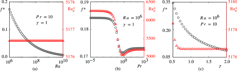
Figure 2: Typical dependence of the critical liquid fraction $f^{\ast}$ and critical effective Rayleigh number ${\textit{Ra}}_{e}^{\ast}$ on (a) Ra with ${\textit{Pr}}=10$ and $\gamma=1$, (b) Pr with $\textit{Ra}=10^{6}$ and $\gamma=1$, and (c) $\gamma$ with $\textit{Ra}=10^{6}$ and ${\textit{Pr}}=10$.

Having derived the transition criterion $f^{\ast}$, we employ it to develop the mathematical model for the melting curve. Following Esfahani et al. (2018); Favier et al. (2019); Yang et al. (2022), we start from the dimensional energy equation for both phases (Voller et al., 1987; Huang et al., 2013a),

$$\frac{\partial{\tilde{T}}}{\partial\tilde{t}}+\boldsymbol{\tilde{u}}\cdot\gradient\tilde{T}={\kappa\nabla^{2}\tilde{T}}-\frac{\mathcal{L}}{C_{p}}\frac{\partial{f_{loc}}}{\partial\tilde{t}},$$ (16)

where $f_{loc}$ represents the local liquid fraction [see (29)] and its volume average is equivalent to the macroscopic counterpart $f$ in (3). The first and last terms represent the change rates of the sensible and latent heats, respectively. The ratio of the two terms, i.e., the Stefan number, is typically far below unity; namely, $\textit{St}=C_{p}\Delta T_{l}/\mathcal{L}\ll 1$, because of the high $\mathcal{L}$ of PCMs. This condition as commonly satisfied in prior studies (Beckermann & Viskanta, 1989; Ho & Gao, 2013; Arasu & Mujumdar, 2012; Kean et al., 2019; Regin et al., 2009; Khan & Khan, 2019), allowing for neglecting the first term.

Further applying Gauss’s theorem, we obtain the integral form of  (16),

$$\frac{\mathcal{L}}{C_{p}}\frac{\partial f}{\partial\tilde{t}}W=\kappa\left[\langle\frac{\partial\tilde{T}}{\partial\tilde{y}}\rangle_{\tilde{y}=W}-\langle\frac{\partial\tilde{T}}{\partial\tilde{y}}\rangle_{\tilde{y}=0}\right],$$ (17)

where $\langle\partial\tilde{T}/\partial\tilde{y}\rangle_{\tilde{y}=W}$, as the average temperature gradient at the cold wall, varies over time generally due to the advancing melting interface. However, in the limit of ${\textit{St}}\ll 1$ as revealed above, the interfacial velocity is negligible compared to the conduction rate, as implied by the normalized Stefan condition $\boldsymbol{\tilde{V}}/({\kappa}/H)={\textit{St}}~(\gradient T_{s}+\gradient T_{l})\cdot\boldsymbol{n}$. Consequently, the conduction process can be considered quasi-steady on the timescale of the interfacial evolution, leading the temperature gradient at the cold wall to

$$\langle\frac{\partial\tilde{T}}{\partial\tilde{y}}\rangle_{\tilde{y}=W}=-\frac{\Delta T_{s}}{W-\tilde{w}},$$ (18)

where $W-\tilde{w}$ quantifies the average thickness of the solid phase (see figure 1a).

At the hot wall, the temperature gradient $\langle\partial\tilde{T}/\partial\tilde{y}\rangle_{\tilde{y}=0}$ depends on the conduction and convection states of the liquid phase. When conduction dominates, this gradient becomes $-\langle\partial\tilde{T}/\partial\tilde{y}\rangle_{\tilde{y}=0}=\Delta T_{l}/\tilde{w}$, which combining  (17) and (18) yields the conduction melting curve in the implicit form

$$\frac{f(1+{\textit{S}}_{T})(f-2{\textit{S}}_{T}+f{\textit{S}}_{T})-2{\textit{S}}_{T}\ln[1-f(1+{\textit{S}}_{T})]}{2(1+{\textit{S}}_{T})^{3}}=\textit{Fo}\textit{St}.$$ (19)

Due to the subcooling effects, this solution differs from the classical Stefan solution $f\sim\sqrt{\textit{Fo}}$ (Esfahani et al., 2018; Fu et al., 2022), but recovers to it when ${\textit{S}}_{T}=0$.

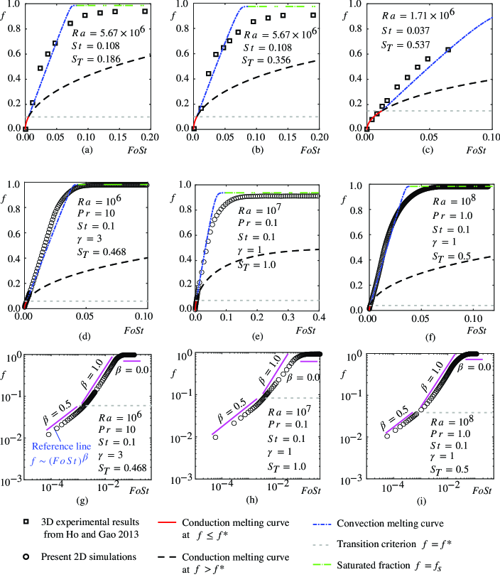
Figure 3: The present model is compared with (a–c) experimental measurements (squares) of n-octadecane ($\textit{Pr}=56$) in a cubic cavity (Ho & Gao, 2013), and (d–f) our two-dimensional numerical data (circles) for a rectangular cavity. The numerical data in (d–f) is represented on a log-log scale in (g–i) to highlight the three melting regimes.

As convection dominates, the temperature gradient can be modelled as $-\langle\partial\tilde{T}/\partial\tilde{y}\rangle_{\tilde{y}=0}={\textit{Nu}}\Delta T_{l}/H$ following (3), resulting in the convection melting curve:

$$\frac{f}{{\textit{Nu}}\gamma}-\frac{{\textit{S}}_{T}}{({\textit{Nu}}\gamma)^{2}}\ln\left[{\textit{Nu}}\gamma(f-1)+{\textit{S}}_{T}\right]=\textit{Fo}\textit{St}+C,$$ (20)

where $C$ is a constant to be determined. Because both melting curves concatenate at $\left({\textit{Fo}}^{\ast}\textit{St},f^{\ast}\right)$, subtracting  (19) from  (20) yields the constant

$$C = \frac{f^{\ast}}{{\textit{Nu}}\gamma}-\frac{{\textit{S}}_{T}}{({\textit{Nu}}\gamma)^{2}}\ln\left[{\textit{Nu}}\gamma(f^{\ast}-1)+{\textit{S}}_{T}\right]$$ (21)

$$- \frac{f^{\ast}(1+{\textit{S}}_{T})(f^{\ast}-2{\textit{S}}_{T}+f^{\ast}{\textit{S}}_{T})-2{\textit{S}}_{T}\ln[1-f^{\ast}(1+{\textit{S}}_{T})]}{2(1+{\textit{S}}_{T})^{3}},$$

where the Nusselt number is expressed using established models, specifically $\textit{Nu}\approx 0.5{\textit{Ra}}^{1/4}{\textit{Pr}}^{1/4}$ for ${\textit{Pr}}\leq 0.1$ and $\textit{Nu}\approx 0.24{\textit{Ra}}^{0.26}{\textit{Pr}}^{0}$ for $\textit{Pr}>0.1$ (Beckermann & Viskanta, 1989; Shishkina, 2016; Wang et al., 2021).

By substituting  (21) into  (20), the domain of the logarithmic function necessitates

$$f<f_{s}=1-\frac{{\textit{S}}_{T}}{{\textit{Nu}}\gamma}.$$ (22)

This indicates that melting will cease at a saturated liquid fraction $f_{s}$, leaving a portion of solid PCM unmelted.

Thus far, we have derived the critical liquid fraction $f^{\ast}$ and established a mathematical model for the melting curve. As shown in figure 3a–c, the theoretical melting curves agree well with the prior experimental data (Ho & Gao, 2013). Besides, these curves also capture the trend revealed in our two-dimensional simulations, see figure 3d–f. In the long-time limit, these curves asymptotically flattens, converging to $f_{s}$ as expected. To better characterize the transition, we depict these curves on a log-log scale in figure 3g–i. The temporal evolution of $f$ exhibits three distinct phases: the first two follow a power-law relationship $f\sim(\textit{Fo}\textit{St})^{\beta}$ with exponents $\beta\approx 0.5$ and $\beta\approx 1.0$, respectively, followed by a saturated phase. Notably, this power-law scaling is exact in no-subcooling cases (${\textit{S}}_{T}=0$), where $\beta=0.5$ and $1.0$ correspond to the conduction-dominated and convection-dominated regimes, respectively (Esfahani et al., 2018; Favier et al., 2019; Li et al., 2022). For present subcooling scenarios (${\textit{S}}_{T}>0$), the first two regimes with different $\beta$ are precisely demarcated by the predicted transition criterion $f=f^{\ast}$ (gray dashed line). Our theory’s predictive ability is further validated through benchmark comparisons with both our simulations and published data (Beckermann & Viskanta, 1989) as detailed in Appendix A.

Despite the generally satisfactory agreement between theoretical predictions and the experimental/numerical data, slight discrepancies are observed. They arise from two approximations: 1) neglecting the time variation of sensible heat in (16) and 2) assuming a steady temperature gradient at the cold wall to obtain (18). Both approximations hold when $\textit{St}\ll 1$. At $\textit{St}=0.1$, figure 3 indicates that the maximum relative error between the theoretical and numerical predictions of $f$ is $\approx 15\%$. This error increases with St, reaching $\approx 20\%$ when $\textit{St}\in\left(0.2,0.4\right)$, see Appendix C.

We now exploit the theoretical melting curve $f(\textit{Fo})$ to predict the key performance indicators. We start with the energy density ED as the cumulative energy stored per unit volume of PCM (Woods et al., 2021; Fu et al., 2022), which depends on the liquid fraction $f$ through

$$\textit{ED}\left(\tilde{t}\right)=\rho[C_{p}(T_{f}-T_{c})+\mathcal{L}]f.$$ (23)

Here, we have neglected the liquid’s sensible heat that plays a negligible role, as demonstrated in Fu et al. (2022) and confirmed by our experimentally-verified calculations (see Appendix E). Notably, the maximum value of ED, reached at $f=f_{s}$, represents the energy storage capacity, whereas the temporal derivative of ED serves as another indicator, the power density (Woods et al., 2021; Fu et al., 2022).

Practically,  (23) characterizes how design parameters of a PCM system affect its performance via the dimensionless numbers encoded in the melting curve. This characterization, requiring only simple algebraic calculations, enables the rapid determination of parameters customized to meet specified performance criteria, thereby streamlining the system’s design.

Besides precisely characterizing performance, the theoretical solutions also provide general guidance for optimizing design parameters. For example, the critical liquid fraction $f^{\ast}$ signifies the duration of the conduction-dominated regime, which features inefficient heat transfer. Hence, reducing $f^{\ast}$ can enhance the melting rate (Sun et al., 2016; Azad et al., 2021a), i.e., the power density. In the current configuration, this can be achieved by increasing the aspect ratio $\gamma$, see (15).

3 Conclusion

By employing linear stability analysis and the integral energy equation, we have developed a theoretical framework for modeling the melting process and performance of PCM systems. Focusing on a exemplary system characterized by lateral heating, we derive an experimentally and numerically validated mathematical model for the melting curve. This curve facilitates rapid designs of PCM systems tailored to specific performance targets. Furthermore, we illustrate, in Appendix D–F, the theoretical framework’s versatility by modelling a variety of other representative PCM configurations, with theoretical predictions corroborated by prior studies (Kean et al., 2019; Korti & Guellil, 2020; Dhaidan et al., 2013). These configurations vary in material species—ranging from pure PCM to nanoparticle-enhanced PCM, in geometries—including an inclined rectangular cavity and an annular tube, and in operational conditions, such as isothermal and constant power heating. Overall, our investigation exemplifies the application of thermo-hydrodynamic theory and physics in facilitating the development of engineering solutions for energy applications.

[Funding]L.Z. acknowledges the partial support received from the National University of Singapore, under the startup grant A-0009063-00-00. The computation of the work was performed on resources of the National Supercomputing Centre, Singapore (https://www.nscc.sg)

[Declaration of interests] The authors report no conflict of interest.

[Author ORCID]Min Li, https://orcid.org/0000-0001-5785-6617; Lailai Zhu, https://orcid.org/0000-0002-3443-0709

Appendix A Numerical Method

In this section, we first present the numerical method used to simulate the melting process of PCM. We then validate the numerical solver using published data.

The numerical simulations of the melting process are performed using the lattice Boltzmann method (Huang et al., 2013a; Luo et al., 2015), which employs density distribution $\eta_{i}$ and temperature distribution $\zeta_{i}$ to describe the evolution of velocity and temperature, respectively. The evolution equations at grid location $\boldsymbol{x}$ are given by:

$$\eta_{i}(\boldsymbol{x}+\boldsymbol{e}_{i},t+1) =\eta_{i}(\boldsymbol{x},t)+\frac{1}{\tau_{v}}\left[\eta_{i}^{eq}(\boldsymbol{x},t)-\eta_{i}(\boldsymbol{x},t)\right]+F_{i},$$ (24a)

$$\zeta_{i}(\boldsymbol{x}+\boldsymbol{e}_{i},t+1) =\zeta_{i}(\boldsymbol{x},t)+\frac{1}{\tau_{T}}\left[\zeta_{i}^{eq}(\boldsymbol{x},t)-\zeta_{i}(\boldsymbol{x},t)\right]+S,$$ (24b)

where $\boldsymbol{e}_{i}$ is the discrete velocity in direction $i$, and $\tau$ with different subscripts represents the dimensionless relaxation time. Here, $F_{i}$ is the discretized body force and $S$ represents the latent heat source. The equilibrium distributions are expressed as

$$\eta_{i}^{eq} =\tilde{\rho}\omega_{i}[1+3\boldsymbol{e}_{i}\cdot\boldsymbol{\tilde{u}}+4.5(\boldsymbol{e}_{i}\cdot\boldsymbol{\tilde{u}})^{2}-1.5\boldsymbol{\tilde{u}}^{2}],$$ (25a)

$$\zeta_{i}^{eq} =\tilde{T}\omega_{i}[1+3\boldsymbol{e}_{i}\cdot\boldsymbol{\tilde{u}}+4.5(\boldsymbol{e}_{i}\cdot\boldsymbol{\tilde{u}})^{2}-1.5\boldsymbol{\tilde{u}}^{2}].$$ (25b)

The weight coefficient in direction $i$ is represented by $w_{i}$ . The density, velocity and temperature are calculated as

$$\tilde{\rho}=\sum_{i}\eta_{i},~\tilde{\rho}\boldsymbol{\tilde{u}}=\sum_{i}\eta_{i}\boldsymbol{e}_{i},~\tilde{T}=\sum_{i}\zeta_{i}.$$ (26)

Notably, all quantities are expressed in lattice units, which can be converted to physical units according to specific rules (Feng et al., 2007; Xia et al., 2024).

The discretized body force in  (24a) reads (Guo & Shu, 2013),

$$F_{i}=3\omega_{i}\boldsymbol{e}_{i}\cdot[-\tilde{\rho}\boldsymbol{g}\alpha(\tilde{T}-T_{0})].$$ (27)

The source term in  (24b) is

$$S=-\omega_{i}\frac{\mathcal{L}}{C_{p}}[{f_{loc}}(\boldsymbol{x},t)-{f_{loc}}(\boldsymbol{x},t-\Delta t)],$$ (28)

which quantifies the propagation effects of melting interface. The local liquid fraction ${f_{loc}}(\boldsymbol{x},t)$ is determined from the enthalpy interpolation

$${f_{loc}}(\boldsymbol{x},t)=\left\{\begin{array}[]{lr}0,&~{\rm if}~\mathcal{H}<\mathcal{H}_{s}=C_{p}T_{f}\\ \frac{\mathcal{H}-\mathcal{H}_{s}}{\mathcal{H}_{l}-\mathcal{H}_{s}},&~{\rm if}~\mathcal{H}_{s}\leq\mathcal{H}\leq\mathcal{H}_{l}=\mathcal{H}_{s}+\mathcal{L}\\ 1,&~{\rm if}~\mathcal{H}>H_{l},\end{array}\right.$$ (29)

where the enthalpy is calculated as $\mathcal{H}=C_{p}\tilde{T}+{f_{loc}}(\boldsymbol{x},t-\Delta t)\mathcal{L}$.

By Chapman-Enskog analysis, the mesoscale evolution equations, (24a) and (24b), recover the macroscopic conservation laws in the limit of low Mach number (Guo & Shu, 2013; Huang et al., 2013a). Additionally, this analysis shows that $\tau_{v}=3\nu+0.5$ and $\tau_{T}=3\kappa+0.5$.

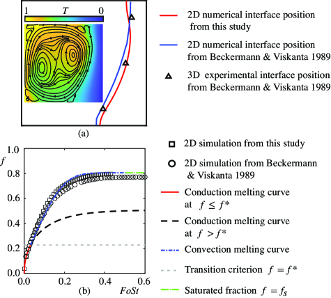
Figure 4: Comparison between our numerical results and those from Beckermann & Viskanta (1989) when ${\textit{Ra}}=4.877\times 10^{5}$, ${\textit{Pr}}=0.0208$, ${\textit{St}}=7.557\times 10^{-2}$, $\gamma=1$, and ${\textit{S}}_{T}=0.971$. (a) Interface position at the end of the melting process, with the inset showing the temperature field and streamlines; (b) liquid fraction $f$ versus FoSt.

Using the above method, we conduct two-dimensional direct numerical simulations for a lateral heating cavity. The non-equilibrium extrapolation scheme (Guo et al., 2002) is implemented to impose both the velocity and temperature boundary conditions. Following previous studies (Favier et al., 2019; Purseed et al., 2020), we assume identical physical properties for the solid and liquid phases.  Additionally, micro-scale Gibbs-Thomson effects are neglected, ensuring $\tilde{T}_{l}=\tilde{T}_{s}=T_{f}$ at the melting interface (Davis et al., 1984; Toppaladoddi & Wettlaufer, 2019; Lu et al., 2022). In figure 4, we compare our numerical results with prior experimental and two-dimensional numerical data (Beckermann & Viskanta, 1989). The demonstrated agreement between the three datasets validates our numerical implementation.

Moreover, the numerical data in figure 4b further validate our derived melting curves and the transition criterion. This indicates that our results are applicable not only to the organic PCM n-octadecane, as discussed in the main article, but also to metallic materials (${\textit{Pr}}=0.0208$ herein corresponding to Gallium (Beckermann & Viskanta, 1989)).

Appendix B A Posterior Justification of Neglecting Advection Term

We neglect the advection terms in (4) to simply the stability analysis, assuming a low Péclect number ($Pe=U_{0}\tilde{w}_{b}/\kappa$) in the conduction-dominated regime. This assumption is validated by examining the evolution of $Pe$ in melting processes of three configurations, as shown in figure 5. Within the conduction-dominated regime ($f<f^{\ast}$), $Pe$ remains low, reaching critical values of 0.22, 0.44, and 0.027 when $f=f^{\ast}$. This directly justifies our low-$Pe$ assumption. Furthermore, the predictive capacity (see figure 3g–i) of the theoretical criterion (15) derived from the simplified perturbation equations indirectly corroborates the neglect of advection terms.

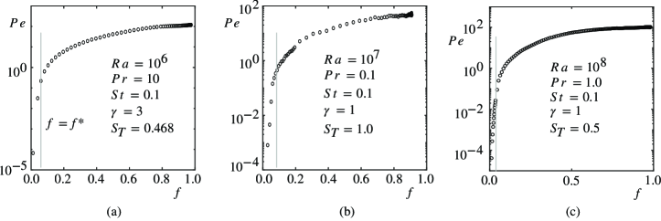
Figure 5: Evolution of Péclet number in three configurations: (a) ${\textit{Ra}}=1.0\times 10^{6}$, ${\textit{Pr}}=10.0$, ${\textit{St}}=0.1$, $\gamma=3$, and ${\textit{S}}_{T}=0.468$; (b) ${\textit{Ra}}=1.0\times 10^{7}$, ${\textit{Pr}}=0.1$, ${\textit{St}}=0.1$, $\gamma=1$, and ${\textit{S}}_{T}=1$; (c) ${\textit{Ra}}=1.0\times 10^{8}$, ${\textit{Pr}}=1.0$, ${\textit{St}}=0.1$, $\gamma=1$, and ${\textit{S}}_{T}=0.5$. The vertical lines represent the critical liquid fraction $f^{\ast}$. These configurations match those in figure 3g–i.

Appendix C Effect of Stefan Number on the Accuracy of the Theoretical Model

As discussed in the main text, our theory assumes $\textit{St}\ll 1$, so its accuracy depends on the value of St. To investigate this dependence, we conduct a series of simulations, as depicted in Figure 6. As expected, the discrepancy between theoretical and numerical predictions increases with growing St for different parametric combinations. Notably, even though the maximum relative error reaches $20\%$, an overall acceptable agreement is seen in figure 6 a, d and g, where $\textit{St}=0.2\sim 0.4$. Thus, we may conclude that the model is valid for $\textit{St}\lessapprox\left(0.2\sim 0.4\right)$. Indeed, most St values in previous studies (Beckermann & Viskanta, 1989; Ho & Gao, 2013; Arasu & Mujumdar, 2012; Kean et al., 2019; Regin et al., 2009; Khan & Khan, 2019) fall within this range, suggesting the relevance of our theoretical model.

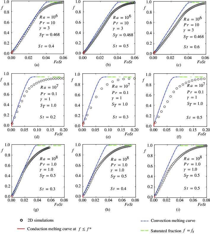
Figure 6: Effects of the Stefan number on the validity of the model, illustrated for different configurations: : (a–c) ${\textit{Ra}}=10^{6}$, ${\textit{Pr}}=10$, $\gamma=3$, and ${\textit{S}}_{T}=0.468$; (d–f) ${\textit{Ra}}=10^{7}$, ${\textit{Pr}}=0.1$, $\gamma=1$, and ${\textit{S}}_{T}=1$; (g–i) ${\textit{Ra}}=10^{8}$, ${\textit{Pr}}=1.0$, $\gamma=1$, and ${\textit{S}}_{T}=0.5$.

Appendix D Melting of Nanoparticle-Enhanced PCM in A Basal Heating Cavity

Here, we apply the theoretical framework to a basal heating configuration, which differs from the lateral heating configuration in two ways. First, the isothermal heat source now serves as the cavity’s bottom wall, instead of the vertical wall. Second, the storage materials are now nanoparticle-enhanced PCM (NEPCM), rather than pure PCM. The analytical solution derived from the theoretical framework successfully predicts the performance of different NEPCMs, despite featuring slightly different material properties. This demonstrates that the framework can accurately evaluate the effects of material properties. With this verified solution, we further provide a new explanation for how nanoparticles affect the melting rate.

D.1 Analytical Solution

The basal heating configuration, shown in figure 7a, can be obtained by simply rotating the lateral heating configuration by 90 degrees in the counter-clockwise direction. This rotation does not alter the energy equation or the dimensionless numbers, as repeated below for completeness,

$$\frac{\partial{\tilde{T}}}{\partial\tilde{t}}+\boldsymbol{\tilde{u}}\cdot\gradient\tilde{T}=\kappa{\nabla^{2}}\tilde{T}-\frac{\mathcal{L}}{C_{p}}\frac{\partial{f_{loc}}}{\partial\tilde{t}},$$ (30)

$${\textit{Ra}}=\frac{g\alpha\Delta T_{l}H^{3}}{\nu\kappa},~{\textit{Pr}}=\frac{\nu}{\kappa},~\textit{St}=\frac{C_{p}\Delta T_{l}}{\mathcal{L}},~{\textit{S}}_{T}=\frac{\Delta T_{s}}{\Delta T_{l}},~\gamma=\frac{W}{H}.$$ (31)

However, the rotation changes the thermal boundary conditions, thus leading to a different melting behavior. Consequently, the Nusselt number Nu, Fourier time Fo, liquid fraction $f$, and effective Rayleigh number $\textit{Ra}_{e}$ are redefined as

Nu $$=-\frac{\tilde{h}}{\Delta T_{l}}\langle\frac{\partial\tilde{T}}{\partial\tilde{x}}\rangle_{\tilde{x}=0},$$ (32a)

Fo $$=\frac{\kappa\tilde{t}}{H^{2}},$$ (32b)

$$f =\frac{\tilde{h}}{H},$$ (32c)

$$\textit{Ra}_{e} =\frac{g\alpha\Delta T_{l}\tilde{h}^{3}}{\nu\kappa}=\textit{Ra}f^{3},$$ (32d)

where $\tilde{h}$ is the average height of the liquid layer, and $\langle~\rangle_{\tilde{x}=0}$ denotes spatial averaging along the hot wall at $\tilde{x}=0$ (figure 7a).

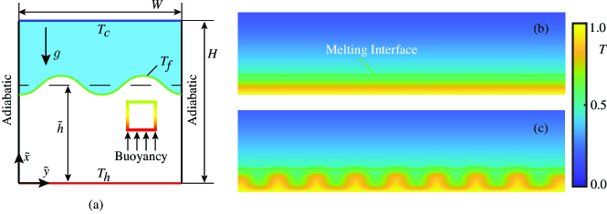
Figure 7: (a) A rectangular cavity filled with subcooled PCM, with the temperature maintained at $T_{h}$ (hot) and $T_{c}$ (cold) at the bottom and top boundaries, respectively. (b) and (c) Typical temperature fields before and after the onset of convection, simulated at $\textit{Ra}=10^{6}$, $\textit{Pr}=10$, $\textit{St}=0.1$, ${\textit{S}}_{T}=1.0$, and $\gamma=2.0$. Only the bottom halves of the fields are presented here.

The transition criterion to differentiate melting regimes in this configuration can be obtained through linear stability analysis. The base flow is $\tilde{\boldsymbol{u}}_{b}=\mathbf{0}$, since the buoyancy is now horizontally homogeneous as indicated by $\partial\tilde{T}/\partial\tilde{y}=0$ (figure 7a). Consequently, the instability phenomenon is very similar to that of the canonical Rayleigh-Bérnard convection (figure 7b and c), and has been extensively investigated (Davis et al., 1984; Kim et al., 2008; Vasil & Proctor, 2011; Esfahani et al., 2018; Madruga & Curbelo, 2018; Favier et al., 2019; Purseed et al., 2020).

For the present configuration, the transition criterion is described by a critical effective Rayleigh number ${\textit{Ra}}_{e}^{\ast}$. It ranges from 1708 to 1493 (Davis et al., 1984), depending on the relative heights of the liquid and solid layers when the melting process is saturated. The highest and lowest ${\textit{Ra}}_{e}^{\ast}$ correspond to similar liquid fractions, as indicated by $\left(1708/1493\right)^{1/3}=1.05$, following  (32d). Thus, the critical liquid fraction $f^{\ast}$ in subsequent theoretical modeling can be approximated by the median value, analogous to the lateral heating configuration

$$f^{\ast}=\left(\frac{1600.5}{{\textit{Ra}}}\right)^{1/3}.$$ (33)

With this transition criterion $f^{\ast}$, we proceed to develop the mathematical model for the melting curve, following the same framework as in the lateral heating configuration. Neglecting the first term of  (30) and applying Gauss’s theorem to the remaining terms, we obtain

$$\frac{\mathcal{L}}{C_{p}}\frac{\partial f}{\partial\tilde{t}}H=\kappa\left[\langle\frac{\partial\tilde{T}}{\partial\tilde{x}}\rangle_{\tilde{x}=H}-\langle\frac{\partial\tilde{T}}{\partial\tilde{x}}\rangle_{\tilde{x}=0}\right].$$ (34)

For the same reasons as in the lateral heating configuration, the temperature gradient at the cold wall can be considered steady, as

$$\langle\frac{\partial\tilde{T}}{\partial\tilde{x}}\rangle_{\tilde{x}=H}=-\frac{\Delta T_{s}}{H-\tilde{h}},$$ (35)

where $H-\tilde{h}$ quantifies the average height of the solid phase (see figure 7a).

At the hot wall, the temperature gradient $\langle\partial\tilde{T}/\partial\tilde{x}\rangle_{\tilde{x}=0}$ depends on the conduction and convection states of the liquid phase. When conduction dominates, this gradient becomes $-\langle\partial\tilde{T}/\partial\tilde{x}\rangle_{\tilde{x}=0}=\Delta T_{l}/\tilde{h}$, which combining  (34) and (35) yields the conduction melting curve

$$\frac{f(1+{\textit{S}}_{T})(f-2{\textit{S}}_{T}+f{\textit{S}}_{T})-2{\textit{S}}_{T}\ln[1-f(1+{\textit{S}}_{T})]}{2(1+{\textit{S}}_{T})^{3}}=\textit{Fo}\textit{St}.$$ (36)

This curve exactly matches that in the lateral heating configurations, since the conduction heat transfer solely depends on molecular motion, which is irrelevant to the orientation of the heat source.

As convection dominates, the temperature gradient can be modelled as $-\langle\partial\tilde{T}/\partial\tilde{x}\rangle_{\tilde{x}=0}={\textit{Nu}}\Delta T_{l}/\tilde{h}$ following  (32a), which rearranges  (34) to

$$\frac{\partial f}{\partial\tilde{t}}=\textit{St}\frac{\kappa}{H^{2}}\left[\frac{\textit{Nu}}{f}-\frac{{\textit{S}}_{T}}{1-f}\right].$$ (37)

The Nusselt number in the present configuration is $\textit{Nu}\approx 0.1\textit{Ra}_{e}^{1/3}=0.1\textit{Ra}^{1/3}f$ (Favier et al., 2019), a typical result predicted by the Grossmann-Lohse theory (Ahlers et al., 2009). Substituting this correlation into  (37), we obtain the convection melting curve:

$$\frac{f\mathcal{F}-{\textit{S}}_{T}\ln(f\mathcal{F}+{\textit{S}}_{T}-\mathcal{F})}{\mathcal{F}^{2}}=\textit{Fo}\textit{St}+C,$$ (38)

where $\mathcal{F}=0.1\textit{Ra}^{1/3}$ and $C$ is a constant to be determined. This curve differs from that in the lateral heating configuration, because the convection heat transfer depends on fluid flow, which in turn is influenced by the orientation of the heat source.

Because both conduction and convection melting curves concatenate at $\left({\textit{Fo}}^{\ast}\textit{St},f^{\ast}\right)$, subtracting  (36) from  (38) yields the constant

$$C=\frac{f^{\ast}\mathcal{F}-{\textit{S}}_{T}\ln(f^{\ast}\mathcal{F}+{\textit{S}}_{T}-\mathcal{F})}{\mathcal{F}^{2}}-\frac{f^{\ast}(1+{\textit{S}}_{T})(f^{\ast}-2{\textit{S}}_{T}+f^{\ast}{\textit{S}}_{T})-2{\textit{S}}_{T}\ln[1-f^{\ast}(1+{\textit{S}}_{T})]}{2(1+{\textit{S}}_{T})^{3}}.$$ (39)

By substituting  (39) into  (38), the domain of the logarithmic function necessitates

$$f<f_{s}=1-\frac{{\textit{S}}_{T}}{\mathcal{F}}.$$ (40)

This indicates that melting will cease at a saturated liquid fraction $f_{s}$, leaving a portion of solid PCM unmelted.

For now, we have derived the analytical solutions for the basal heating configuration, using the theoretical framework outlined in the main article for the lateral heating configuration. These solutions are independent of the cavity’s aspect ratio $\gamma$, whereas those for the lateral configuration depend on $\gamma$. In the following, we will verify the new solutions by the results of Kean et al. (2019).

D.2 Verification of the Analytical Solutions

The NEPCM used in Kean et al. (2019) consists of paraffin wax and various concentrations of ${\rm Al}_{2}{\rm O}_{3}$ nanoparticles, which can address the poor thermal conductivity of traditional PCMs (Kibria et al., 2015; Levin et al., 2013; Jebasingh & Arasu, 2020; Yang et al., 2020; Tariq et al., 2020). The thermophysical properties of paraffin wax, ${\rm Al}_{2}{\rm O}_{3}$ nanoparticles, and NEPCM are summarized in Table 1. Here, an experimentally fitted model is utilized to calculate the NEPCM’s density $\rho$, specific heat $C_{p}$, latent heat $\mathcal{L}$, dynamic viscosity $\mu$, and thermal conductivity $K$ (Chow et al., 1996; Vajjha et al., 2010), as

Property	Paraffin wax	${\rm Al}_{2}{\rm O}_{3}$	Wax + $2\%$ ${\rm Al}_{2}{\rm O}_{3}$	Wax + $5\%$ ${\rm Al}_{2}{\rm O}_{3}$
Density ($\rm Kg/m^{3}$)	$\frac{750}{0.001(\tilde{T}-319.15)+1}$	3600	802.36	888.00
Specific heat ($\rm J/(KgK)$)	2890	765	2699.31	2459.26
Latent heat ($\rm J/Kg$)	173400	–	157839.94	138251.52
Thermal conductivity ($\rm W/mK$)	0.12	36	0.16	0.17
Dynamic viscosity ($\rm Kg/ms$)	$0.001\exp(1790/\tilde{T}-4.25)$	–	0.0044	0.0066
Fusion temperature ($\rm K$)	321	–	–	–
Thermal expansion ($\rm 1/K$)	$10^{-3}$	–	–	–

Table 1: Properties of paraffin wax, ${\rm Al}_{2}{\rm O}_{3}$ nanoparticles, and two different NEPCMs (Arasu & Mujumdar, 2012; Kean et al., 2019).

$$\rho =\Psi\rho_{np}+(1-\Psi)\rho_{pw},$$ (41a)

$$C_{p} =\frac{\Psi(\rho c_{p})_{np}+(1-\Psi)(\rho C_{p})_{pw}}{\rho},$$ (41b)

$$\mathcal{L} =\frac{(1-\Psi)(\rho\mathcal{L})_{pw}}{\rho},$$ (41c)

$$\mu =0.983\exp(12.959\Psi)\mu_{pw},$$ (41d)

$$K =\frac{K_{np}+2K_{pw}-2(K_{pw}-K_{np})\Psi}{K_{np}+2K_{pw}+(K_{pw}-K_{np})\Psi}K_{pw}+5\times 10^{4}\beta_{k}\zeta\Psi(\rho C_{p})_{pw}\sqrt{\frac{1.381\times 10^{-23}\tilde{T}}{\rho_{np}d_{np}}}m,$$ (41e)

where $\Psi$ represents the volume fraction of nanoparticles; here, the subscripts ‘${\it pw}$’ and ‘${\it np}$’ denote paraffin wax and ${\rm Al}_{2}{\rm O}_{3}$ nanoparticles, respectively. In  (41e), $d_{np}$ denotes the nanoparticle diameter, and $\zeta$ is a correction factor equal to the local liquid fraction, and $\beta_{k}$ and $m$ are expressed by

$$\beta_{k} =8.4407(100\Psi)^{-1.07304},$$

$$m =(2.8217\times 10^{-2}\Psi+3.917\times 10^{-3})\frac{T}{273}-(3.0669\times 10^{-2}\Psi+3.91123\times 10^{-3}).$$ (42)

In Kean et al. (2019), the cavity dimensions are $W=H=0.025~{\rm m}$, and $d_{np}=59~{\rm nm}$. The temperatures at hot and cold walls are $T_{h}=330~{\rm K}$ and $T_{c}=300~{\rm K}$, respectively. The properties of the NEPCM depend on the temperature field $\tilde{T}$, which can be obtained by simulations but poses a challenge in model calculations. Consequently, we choose the reference temperature $T_{0}=(T_{h}+T_{f})/2$ as the characteristic value of $\tilde{T}$. At this characteristic temperature, the properties of the NEPCM can be calculated using (41) and (42), as listed in Table 1. Notably, other characteristic temperatures, such as $T_{h}$ or $T_{f}$, will not significantly affect the results.

With the properties listed in Table 1, the dimensionless numbers in (31) can be calculated for pure paraffin wax, NEPCM with $2\%$ ${\rm Al}_{2}{\rm O}_{3}$, and NEPCM with $5\%$ ${\rm Al}_{2}{\rm O}_{3}$. The resulting three sets of numbers can then be substituted into the analytical solutions, (33), (36), (38), and (40), to generate three melting curves. As shown in figure 8, these curves agree with the numerical data of Kean et al. (2019), thereby verifying our theoretical solutions. With these verified solutions, we will further discuss the effects of nanoparticles on the melting rate.

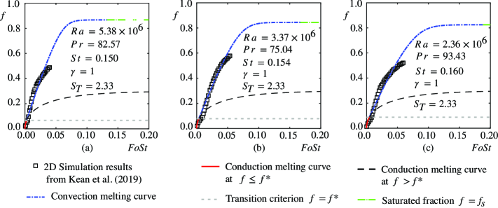
Figure 8: Comparison between our theoretical prediction and numerical results (squares) of Kean et al. (2019) for a cavity filled with: (a) Pure paraffin wax, (b) NEPCM with $2\%$ ${\rm Al}_{2}{\rm O}_{3}$, and (c) NEPCM with $5\%$ ${\rm Al}_{2}{\rm O}_{3}$.

D.3 Effects of Nanoparticles on Melting Rate

According to (38), the dimensionless melting times FoSt to achieve $f=0.5$ are 0.0332, 0.0399, and 0.0462 for pure paraffin wax, NEPCM with $2\%$ ${\rm Al}_{2}{\rm O}_{3}$, and NEPCM with $5\%$ ${\rm Al}_{2}{\rm O}_{3}$, respectively. Correspondingly, the dimensional times $\tilde{t}=\textit{Fo}H^{2}/\kappa$ are 2480.3 s, 2197.9 s, and 2285.7 s, confirming the numerically revealed guideline that NEPCM with $2\%$ ${\rm Al}_{2}{\rm O}_{3}$ exhibits the optimal melting rate  (Kean et al., 2019). This demonstrates that although pure paraffin wax, NEPCM with $2\%$ ${\rm Al}_{2}{\rm O}_{3}$, and NEPCM with $5\%$ ${\rm Al}_{2}{\rm O}_{3}$ have slightly different properties (Table 1), their performance can be accurately differentiated by the present model.

The nonmonotonic dependence of the melting rate on $\Psi$ is widely attributed to the competition between $\mu$ and $K$ (Ho et al., 2008, 2010; Ho & Gao, 2013; Arasu & Mujumdar, 2012; Kibria et al., 2015). When $\Psi$ increases, both $K$ and $\mu$ of NEPCM are enlarged. These studies argued that a larger $K$ enhances heat transfer thus benefits melting, while an augmented $\mu$ hinders heat convection and hence degenerates melting. These opposing effects collectively lead to a nonmonotonic variation in melting rate with $\Psi$. Despite its general acceptance, this explanation might lack rigor. According to ${\textit{Ra}}={g\alpha\Delta T_{l}H^{3}}/{(\nu\kappa)}={g\alpha\Delta T_{l}H^{3}\rho^{2}C_{p}}/{(\mu K)}$, increasing $K$ and $\mu$ both decrease Ra, thereby diminishing convection and negatively impacting melting. This indicates that the effects of $K$ and $\mu$ are not always antagonistic, contrary to the reported explanation. Additionally, nanoparticles not only affect $K$ and $\mu$ but also change $\rho$, $C_{p}$, and $\mathcal{L}$, as illustrated in Table 1. Thus, the reported explanation, which only considers $K$ and $\mu$ in competition, might not fully elucidate the impacts of nanoparticles on the melting rate.

On the other hand, our model offers a more rigorous explanation for the nonmonotonic relation. Our analytical solution, (36) and (38), shows that the melting rate depends on three dimensionless parameters, Ra, St, and ${\textit{S}}_{T}$. Because the fusion temperature $T_{f}$ barely changes with $\Psi$ (Yang et al., 2020), the impact of ${\textit{S}}_{T}$ can be safely neglected, allowing us to focus on Ra and St only. As depicted in figure 8, increasing $\Psi$ decreases Ra and increases St simultaneously. A lower Ra weakens convection, thereby impeding melting. Conversely, a higher $\textit{St}=C_{p}\Delta T_{l}/\mathcal{L}$ signifies a lower latent heat, hence accelerating melting. These two contrasting trends thus result in the nonmonotonic dependence of the melting rate on $\Psi$. The expressions for Ra and St include all the properties affected by nanoparticles, i.e., $K$, $\mu$, $\rho$, $C_{p}$, and $\mathcal{L}$. Hence, compared to the reported explanation, our explanation based on Ra and St encodes a more comprehensive account of how nanoparticles influence the melting rate.

Appendix E Melting of PCM in An Inclined Cavity

This section illustrates the application of the theoretical framework in the configuration of an inclined cavity. Compared to the lateral heating configuration, this configuration has a distinct geometric feature characterized by the inclined angle. Moreover, the heat source in this configuration operates at a constant power, rather than maintaining an isothermal temperature. Despite these differences, the melting curve for the current configuration can be derived using the same theoretical framework. Thus, it is reasonable to claim that the theoretical framework is capable of considering the effects of various geometric features and operational conditions. Using the resulting curve, we further calculate the storage energy, which is consistent with the experimental data (Korti & Guellil, 2020), confirming the effectiveness of the framework in predicting the overall system performance.

The inclined cavity investigated here matches that in Korti & Guellil (2020), as shown in figure 9a. Such an inclined setting is typically encountered when PCM containers are deployed on the non-flat surface of a working device (Khan & Singh, 2024). The dimensions of this cavity are $L=0.045~{\rm m}$ in depth, $W=0.12~{\rm m}$ in width, and $H=0.12~{\rm m}$ in height. All its walls are insulated except for the bottom one, which receives heat from a parallel electrical heater operating at a constant power of $q=2700~{\rm W/m^{2}}$. These thermal boundary conditions are frequently encountered in applications such as electronic cooling and solar energy collection. The entire system can rotate by an angle $\theta$ (figure 9a), and maintains this orientation. The PCM (paraffin wax, CAS 8002-74-2) is initially in the solid phase at a temperature of $T_{c}=296.65~{\rm K}$. The thermophysical properties of the PCM are summarized in Table 2.

Property	Value
Density ($\rm Kg/m^{3}$)	916
Specific heat ($\rm J/KgK$)	2900
Specific latent heat ($\rm J/Kg$)	176000
Thermal conductivity ($\rm W/mK$)	0.12
Dynamic viscosity ($\rm Kg/ms$)	0.0036
Fusion temperature ($\rm K$)	324.65
Thermal expansion ($\rm 1/K$)	$9.1\times 10^{-4}$

Table 2: Properties of the paraffin wax, CAS 8002-74-20(Korti & Guellil, 2020).

Using the same framework as applied to the lateral heating cavity, the melting curve for the inclined cavity can be derived as follows. By neglecting the sensible heat term in (16) and applying Gauss’s theorem to the remaining terms, we obtain:

$$\frac{\mathcal{L}}{C_{p}}\frac{\partial f}{\partial\tilde{t}}WH=\int(\kappa\gradient\tilde{T})_{\tilde{x}=0}\cdot\boldsymbol{n}{\rm d}A.$$ (43)

The area element at the bottom wall is ${\rm d}A={\rm d}y\times 1$, with $\boldsymbol{n}=(-1,~0)$ representing the outward unit normal vector (figure 9a). The temperature gradient at this wall $(\gradient\tilde{T})_{\tilde{x}=0}$ can be related to the heater’s power $q$, as explained below.

The PCM container is separated from the electrical heater by a small gap, within which vertical air plumes arise due to buoyancy (figure 9a). Receiving it from the heater, the plumes transfer the heat to the cavity when they impinge on the bottom wall. Thus, during the impingement process, we obtain:

$$-\rho C_{p}\kappa(\gradient\tilde{T})_{\tilde{x}=0}=q(\cos\theta,~\sin\theta),$$ (44)

where the right-hand side represents the heat flux carried by the plumes, as shown in figure 9a. This equation indicates that the wall temperature gradient does not depend on the conduction and convection melting regimes. Therefore, linear stability analysis, which is required in the lateral heating configuration to distinguish different regimes, is not necessary in this configuration.

Based on (44), the integration of wall temperature gradient can be calculated as

$$\int(\kappa\gradient\tilde{T})_{\tilde{x}=0}\cdot\boldsymbol{n}{\rm d}A=\int_{0}^{W}\frac{q}{\rho C_{p}}\cos\theta{\rm d}y=\frac{q\cos\theta}{\rho C_{p}}W.$$ (45)

Subsequently, the melting curve can be obtained from (43), as

$$f=t\cos\theta,$$ (46)

where the dimensionless time is $t=q\tilde{t}/(\rho H\mathcal{L})$. This curve does not impose any constraint on the liquid fraction $f$. Thus, its saturated value is $f_{s}=1$, indicating that the solid PCM can be completely melted. Notably, at a large inclination, e.g., $\theta\geq\pi/2$, the vertical air plumes do not impinge on the bottom wall. Accordingly, (44) no longer holds, and determining $(\gradient\tilde{T})_{\tilde{x}=0}$ would require analysis of the flow field within the gap. This is beyond the scope of this study, which is hence not pursued here.

Figure 9: (a) An inclined cavity filled with subcooled PCM, with the bottom wall heated by a parallel electrical heater. (b) and (c) Comparison between the melting curve and the experimental results (Korti & Guellil, 2020), when the inclination angle $\theta=0$ and $\pi/4$, respectively. (d) and (e), similar to (b) and (c), but for the storage energy.

According to (46), the derived melting curve accounts for the effects of material properties ($\rho$ and $\mathcal{L}$), geometric features ($H$ and $\theta$), and operational condition ($q$). This curve is well-verified against the experimental results (Korti & Guellil, 2020) at $\theta=0$ and $\theta=\pi/4$, as shown in in figures 9b and c. This verified curve can then be used to calculate the energy density (23).  The energy density ED, when multiplied by the container volume ($W\times H\times L$), yields the storage energy, which is consistent with the experimental result (figures 9d and e), thereby confirming the model’s effectiveness. The power density is the time derivative of ED, which is hence not verified here separately.

Appendix F Melting of PCM in An Annular Tube

Here, we apply the theoretical framework to the configuration of an annular tube. This configuration differs significantly from the lateral heating configuration in terms of the container’s geometry. Moreover, the heat source in this configuration operates at constant power, rather than maintaining an isothermal temperature. Despite these differences, the melting curve for the current configuration can be derived using the same theoretical framework. This curve is well validated by the experimental results (Dhaidan et al., 2013), confirming the capability of the theoretical framework to account for the effects of various geometric features and operational conditions.

The configuration of the annular tube is the same as that in Dhaidan et al. (2013), as shown in figure 10a. In this setup, the outer shell and inner tube are coaxially arranged with radii of of $R_{o}=22.25~{\rm mm}$ and $R_{i}=9.5~{\rm mm}$, respectively. The outer shell is insulated, while the inner tube is heated by an electrical heater operating at a constant power $q$. The space between the shell and tube contains n-octadecane paraffin. Initially, this PCM is in the solid phase at a temperature of $T_{c}=295.85~{\rm K}$, and its thermophysical properties are summarized in Table 3.

Property	Value
Density ($\rm Kg/m^{3}$)	770
Specific heat ($\rm J/KgK$)	2196
Specific latent heat ($\rm J/Kg$)	243500
Thermal conductivity ($\rm W/mK$)	0.148
Kinematic viscosity ($\rm m^{2}/s$)	$5\times 10^{-6}$
Fusion temperature ($\rm K$)	301.15
Thermal expansion ($\rm 1/K$)	$9.1\times 10^{-4}$

Table 3: Properties of n-octadecane paraffin (Dhaidan et al., 2013).

Following the same framework outlined in the main article, the melting curve for this annular tube is derived as follows. By neglecting the sensible heat term in (16) and applying Gauss’s theorem to the remaining terms, we obtain:

$$\frac{\mathcal{L}}{C_{p}}\frac{\partial f}{\partial\tilde{t}}(\pi R_{o}^{2}-R_{i}^{2})=\int(\kappa\gradient\tilde{T})_{\tilde{r}=R_{i}}\cdot\boldsymbol{n}{\rm d}A.$$ (47)

The area element of the tube wall is ${\rm d}A={\rm d}\theta R_{i}\times 1$, with $\boldsymbol{n}=(-\cos\theta,~-\sin\theta)$ representing the outward unit normal vector (figure 10a). The temperature gradient at this wall $(\gradient\tilde{T})_{\tilde{r}=R_{i}}$ can be related to the heater’s power $q$, as shown below.

The inner tube is separated from the electrical heater by a small gap, within which vertical air plumes arise due to buoyancy (figure 10a). These plumes receive heat from the heater, and then transfer it to the upper half of the inner tube when they impinge on the tube wall. Thus, during the impingement process, we obtain:

$$-\rho C_{p}\kappa(\gradient\tilde{T})_{\tilde{r}=R_{i}}=q(0,~1),$$ (48)

where the right-hand side represents the heat flux carried by the plumes, as shown in figure 10a. This equation indicates that the wall temperature gradient does not depend on the conduction and convection melting regimes. Therefore, linear stability analysis is not necessary here.

Using (48), the integration of wall temperature gradient can be calculated by

$$\int(\kappa\gradient\tilde{T})_{\tilde{r}=R_{i}}\cdot\boldsymbol{n}{\rm d}A=\int_{0}^{\pi}\frac{q}{\rho C_{p}}\sin\theta~R_{i}{\rm d}\theta=\frac{2R_{i}q}{\rho C_{p}}.$$ (49)

Subsequently, the melting curve can be obtained from (47) as

$$f=t,$$ (50)

where the dimensionless time is $t=2R_{i}q\tilde{t}/[\pi\rho\mathcal{L}(R_{o}^{2}-R_{i}^{2})]$. This curve does not impose any constraint on $f$. Thus, the saturated value should be $f_{s}=1$, indicating that the solid PCM can be completely melted.

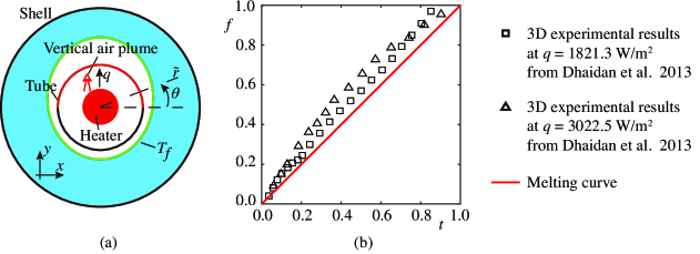
Figure 10: (a) An annular tube filled with subcooled PCM. (b) Comparison between our predicted melting curve and the experimental results (Dhaidan et al., 2013).

According to (50), the derived melting curve accounts for the effects of material properties ($\rho$ and $\mathcal{L}$), geometric features ($R_{i}$ and $R_{o}$), and operational condition ($q$). Figure 10b suggests that this curve agrees reasonably well with the experimental data (Dhaidan et al., 2013) when $q=1821.3~{\rm W/m^{2}}$ and $q=3022.5~{\rm W/m^{2}}$, verifying our theoretical solutions.

References

- Ahlers et al. (2022) Ahlers, G., Bodenschatz, E., Hartmann, R., He, X., Lohse, D., Reiter, P., Stevens, R. J. A. M., Verzicco, R., Wedi, M., Weiss, S. & others 2022 Aspect ratio dependence of heat transfer in a cylindrical Rayleigh-Bénard cell. Phys. Rev. Lett. 128 (8), 084501.
- Ahlers et al. (2009) Ahlers, G., Grossmann, S. & Lohse, D. 2009 Heat transfer and large scale dynamics in turbulent Rayleigh-Bénard convection. Rev. Mod. Phys. 81 (2), 503.
- Arasu & Mujumdar (2012) Arasu, A. V. & Mujumdar, A. S. 2012 Numerical study on melting of paraffin wax with Al2O3 in a square enclosure. Int. Commun. Heat Mass 39 (1), 8–16.
- Azad et al. (2021a) Azad, M., Groulx, D. & Donaldson, A. 2021a Natural convection onset during melting of phase change materials: Part I–effects of the geometry, Stefan number, and degree of subcooling. Int. J. Therm. Sci. 170, 107180.
- Azad et al. (2021b) Azad, M., Groulx, D. & Donaldson, A. 2021b Natural convection onset during melting of phase change materials: Part II–effects of Fourier, Grashof, and Rayleigh numbers. Int. J. Therm. Sci. 170, 107062.
- Azad et al. (2022) Azad, M., Groulx, D. & Donaldson, A. 2022 Natural convection onset during melting of phase change materials: Part III–global correlations for onset conditions. Int. J. Therm. Sci. 172, 107368.
- Beckermann & Viskanta (1989) Beckermann, C. & Viskanta, R. 1989 Effect of solid subcooling on natural convection melting of a pure metal. J. Heat Transfer 111, 416–424.
- Chen et al. (2022) Chen, X., Liu, P., Gao, Y. & Wang, G. 2022 Advanced pressure-upgraded dynamic phase change materials. Joule 6 (5), 953–955.
- Chow et al. (1996) Chow, L. C., Zhong, J. K. & Beam, J. E. 1996 Thermal conductivity enhancement for phase change storage media. Int. Commun. Heat Mass 23 (1), 91–100.
- Davis et al. (1984) Davis, S. H., Müller, U. & Dietsche, C. 1984 Pattern selection in single-component systems coupling Bénard convection and solidification. J. Fluid Mech. 144, 133–151.
- Dhaidan & Khodadadi (2015) Dhaidan, N. S. & Khodadadi, J. M. 2015 Melting and convection of phase change materials in different shape containers: A review. Renew. Sust. Energ. Rev. 43, 449–477.
- Dhaidan et al. (2013) Dhaidan, N. S., Khodadadi, J. M., Al-Hattab, T. A. & Al-Mashat, S. M. 2013 Experimental and numerical investigation of melting of NePCM inside an annular container under a constant heat flux including the effect of eccentricity. Int. J. Heat Mass Transf. 67, 455–468.
- Duan et al. (2019) Duan, J., Xiong, Y. & Yang, D. 2019 On the melting process of the phase change material in horizontal rectangular enclosures. Energies 12 (16), 3100.
- Dutil et al. (2011) Dutil, Y., Rousse, D. R., Salah, N. B., Lassue, S. & Zalewski, L. 2011 A review on phase-change materials: Mathematical modeling and simulations. Renew. Sust. Energ. Rev. 15 (1), 112–130.
- Esfahani et al. (2018) Esfahani, B. R., Hirata, S. C., Berti, S. & Calzavarini, E. 2018 Basal melting driven by turbulent thermal convection. Phys. Rev. Fluids 3 (5), 053501.
- Favier et al. (2019) Favier, B., Purseed, J. & Duchemin, L. 2019 Rayleigh-Bénard convection with a melting boundary. J. Fluid Mech. 858, 437–473.
- Feng et al. (2007) Feng, Y. T., Han, K. & Owen, D. R. J. 2007 Coupled lattice boltzmann method and discrete element modelling of particle transport in turbulent fluid flows: Computational issues. Int. J. Numer. Methods Eng. 72 (9), 1111–1134.
- Fu et al. (2022) Fu, W., Yan, X., Gurumukhi, Y., Garimella, V. S., King, W. P. & Miljkovic, N. 2022 High power and energy density dynamic phase change materials using pressure-enhanced close contact melting. Nat. Energy 7 (3), 270–280.
- Gao & Lu (2021) Gao, T. & Lu, W. 2021 Machine learning toward advanced energy storage devices and systems. iScience 24 (1), 101936.
- Gau & Viskanta (1986) Gau, C. & Viskanta, R. 1986 Melting and solidification of a pure metal on a vertical wall. J. Heat Transfer 108, 174–181.
- Gerkman & Han (2020) Gerkman, M. A. & Han, G. G. D. 2020 Toward controlled thermal energy storage and release in organic phase change materials. Joule 4 (8), 1621–1625.
- Guo & Shu (2013) Guo, Z. & Shu, C. 2013 Lattice Boltzmann Method and Its Application in Engineering, , vol. 3. World Scientific.
- Guo et al. (2002) Guo, Z.-L., Zheng, C.-G. & Shi, B.-C. 2002 Non-equilibrium extrapolation method for velocity and pressure boundary conditions in the lattice Boltzmann method. Chinese Phys. 11 (4), 366.
- Gur et al. (2012) Gur, I., Sawyer, K. & Prasher, R. 2012 Searching for a better thermal battery. Science 335 (6075), 1454–1455.
- He et al. (2022) He, Z., Guo, W. & Zhang, P. 2022 Performance prediction, optimal design and operational control of thermal energy storage using artificial intelligence methods. Renew. Sust. Energ. 156, 111977.
- Ho et al. (2008) Ho, C.-J., Chen, M. W. & Li, Z. W. 2008 Numerical simulation of natural convection of nanofluid in a square enclosure: effects due to uncertainties of viscosity and thermal conductivity. Int. J. Heat Mass Transf. 51 (17-18), 4506–4516.
- Ho & Gao (2013) Ho, C.-J. & Gao, J. Y. 2013 An experimental study on melting heat transfer of paraffin dispersed with Al2O3 nanoparticles in a vertical enclosure. Int. J. Heat Mass Transf. 62, 2–8.
- Ho et al. (2010) Ho, C. J., Liu, W. K., Chang, Y. S. & Lin, C. C. 2010 Natural convection heat transfer of alumina-water nanofluid in vertical square enclosures: An experimental study. IInt. J. Therm. Sci. 49 (8), 1345–1353.
- Ho & Viskanta (1984) Ho, C-J & Viskanta, R 1984 Heat transfer during melting from an isothermal vertical wall. J. Heat Transfer 106, 12–19.
- Huang et al. (2013a) Huang, R., Wu, H. & Cheng, P. 2013a A new lattice Boltzmann model for solid–liquid phase change. Int. J. Heat Mass Transf. 59, 295–301.
- Huang et al. (2013b) Huang, S.-D., Kaczorowski, M., Ni, R., Xia, K.-Q. & others 2013b Confinement-induced heat-transport enhancement in turbulent thermal convection. Phys. Rev. Lett. 111 (10), 104501.
- Huang & Xia (2016) Huang, S.-D. & Xia, K.-Q. 2016 Effects of geometric confinement in quasi-2-D turbulent Rayleigh-Bénard convection. J. Fluid Mech. 794, 639–654.
- Jebasingh & Arasu (2020) Jebasingh, B. E. & Arasu, A. V. 2020 A comprehensive review on latent heat and thermal conductivity of nanoparticle dispersed phase change material for low-temperature applications. Energy Storage Mater. 24, 52–74.
- Kean et al. (2019) Kean, T. H., Sidik, N. A. C. & Kaur, J. 2019 Numerical investigation on melting of phase change material (PCM) dispersed with various nanoparticles inside a square enclosure. In IOP Conf. Ser. Mater. Sci. Eng., , vol. 469, p. 012034. IOP Publishing.
- Khan & Singh (2024) Khan, J. & Singh, P. 2024 Review on phase change materials for spacecraft avionics thermal management. J. Energy Storage 87, 111369.
- Khan & Khan (2019) Khan, Z. & Khan, Z. A. 2019 Thermodynamic performance of a novel shell-and-tube heat exchanger incorporating paraffin as thermal storage solution for domestic and commercial applications. Appl. Therm. Eng. 160, 114007.
- Kibria et al. (2015) Kibria, M. A., Anisur, M. R., Mahfuz, M. H., Saidur, R. & Metselaar, I. H. S. C. 2015 A review on thermophysical properties of nanoparticle dispersed phase change materials. Energ. Convers. Manage. 95, 69–89.
- Kim et al. (2008) Kim, M. C., Lee, D. W. & Choi, C. K. 2008 Onset of buoyancy-driven convection in melting from below. Korean J. Chem. Eng. 25 (6), 1239–1244.
- Kishore et al. (2023) Kishore, R. A., Mahvi, A., Singh, A. & Woods, J. 2023 Finned-tube-integrated modular thermal storage systems for hvac load modulation in buildings. Cell Rep. Phys. Sci. 4 (12), 101704.
- Korti & Guellil (2020) Korti, A. I. N. & Guellil, H. 2020 Experimental study of the effect of inclination angle on the paraffin melting process in a square cavity. J. Energy Storage 32, 101726.
- Lachheb et al. (2024) Lachheb, M., Younsi, Z., Youssef, N. & Bouadila, S. 2024 Enhancing building energy efficiency and thermal performance with PCM-integrated brick walls: A comprehensive review. Build. Environ. p. 111476.
- Levin et al. (2013) Levin, P. P., Shitzer, A. & Hetsroni, G. 2013 Numerical optimization of a PCM-based heat sink with internal fins. Int. J. Heat Mass Transf. 61, 638–645.
- Li et al. (2022) Li, M., Jiao, Z. & Jia, P. 2022 Melting processes of phase change materials in a horizontally placed rectangular cavity. J. Fluid Mech. 950, A34.
- Li & Su (2023) Li, Y. & Su, G. 2023 Melting processes of phase change material in sidewall-heated cavity. J. Thermophys. Heat Transfer 37 (2), 513–518.
- Liu et al. (2022) Liu, Y., Zheng, R. & Li, J. 2022 High latent heat phase change materials (PCMs) with low melting temperature for thermal management and storage of electronic devices and power batteries: Critical review. Renew. Sust. Energ. 168, 112783.
- Lu et al. (2022) Lu, C., Zhang, M., Luo, K., Wu, J. & Yi, H. 2022 Rayleigh-Bénard instability in the presence of phase boundary and shear. J. Fluid Mech. 948, A46.
- Luo et al. (2015) Luo, K., Yao, F.-J., Yi, H.-L. & Tan, H.-P. 2015 Lattice Boltzmann simulation of convection melting in complex heat storage systems filled with phase change materials. Appl. Therm. Eng. 86, 238–250.
- Madruga & Curbelo (2018) Madruga, S. & Curbelo, J. 2018 Dynamic of plumes and scaling during the melting of a phase change material heated from below. Int. J. Heat Mass Transf. 126, 206–220.
- Purseed et al. (2020) Purseed, J., Favier, B., Duchemin, L. & Hester, E. W. 2020 Bistability in Rayleigh-Bénard convection with a melting boundary. Phys. Rev. Fluids 5 (2), 023501.
- Ragoowansi et al. (2023) Ragoowansi, E. A., Garimella, S. & Goyal, A. 2023 Realistic utilization of emerging thermal energy recovery and storage technologies for buildings. Cell Rep. Phys. Sci. 4 (5), 101393.
- Regin et al. (2009) Regin, A. F., Solanki, S. C. & Saini, J. S. 2009 An analysis of a packed bed latent heat thermal energy storage system using PCM capsules: Numerical investigation. Renew. Energy 34 (7), 1765–1773.
- Shishkina (2016) Shishkina, O. 2016 Momentum and heat transport scalings in laminar vertical convection. Phys. Rev. E 93 (5), 051102.
- Shishkina (2021) Shishkina, O. 2021 Rayleigh-Bénard convection: The container shape matters. Phys. Rev. Fluids 6 (9), 090502.
- Sun et al. (2016) Sun, X., Zhang, Q., Medina, M. A. & Lee, K. O. 2016 Experimental observations on the heat transfer enhancement caused by natural convection during melting of solid–liquid phase change materials (PCMs). Appl. Energy 162, 1453–1461.
- Tariq et al. (2020) Tariq, S. L., Ali, H. M., Akram, M. A., Janjua, M. M. & Ahmadlouydarab, M. 2020 Nanoparticles enhanced phase change materials (NePCMs)-A recent review. Appl. Therm. Eng. 176, 115305.
- Tong et al. (2021) Tong, S., Nie, B., Li, Z., Li, C., Zou, B., Jiang, L., Jin, Y. & Ding, Y. 2021 A phase change material (PCM) based passively cooled container for integrated road-rail cold chain transportation—an experimental study. Appl. Therm. Eng. 195, 117204.
- Toppaladoddi & Wettlaufer (2019) Toppaladoddi, S. & Wettlaufer, J. S. 2019 The combined effects of shear and buoyancy on phase boundary stability. J. Fluid Mech. 868, 648–665.
- Vajjha et al. (2010) Vajjha, R. S., Das, D. K. & Namburu, P. K. 2010 Numerical study of fluid dynamic and heat transfer performance of Al2O3 and CuO nanofluids in the flat tubes of a radiator. Int. J. Heat Fluid Fl. 31 (4), 613–621.
- Vasil & Proctor (2011) Vasil, G. M. & Proctor, M. R. E. 2011 Dynamic bifurcations and pattern formation in melting-boundary convection. J. Fluid Mech. 686, 77–108.
- Verma et al. (2008) Verma, P., Singal, S. K. & others 2008 Review of mathematical modeling on latent heat thermal energy storage systems using phase-change material. Renew. Sustain. Energy Rev. 12 (4), 999–1031.
- Vogel et al. (2016) Vogel, J., Felbinger, J. & Johnson, M. 2016 Natural convection in high temperature flat plate latent heat thermal energy storage systems. Appl. Energy 184, 184–196.
- Voller et al. (1987) Voller, V. R., Cross, M. & Markatos, N. C. 1987 An enthalpy method for convection/diffusion phase change. Int. J. Numer. Methods Biomed. Eng. 24 (1), 271–284.
- Wang et al. (2012) Wang, B.-F., Ma, D.-J., Chen, C. & Sun, D.-J. 2012 Linear stability analysis of cylindrical Rayleigh-Bénard convection. J. Fluid Mech. 711, 27–39.
- Wang et al. (2022a) Wang, H., Peng, Y., Peng, H. & Zhang, J. 2022a Fluidic phase–change materials with continuous latent heat from theoretically tunable ternary metals for efficient thermal management. Proc. Natl. Acad. Sci. U.S.A. 119 (31), e2200223119.
- Wang et al. (2021) Wang, Q., Liu, H.-R., Verzicco, R., Shishkina, O. & Lohse, D. 2021 Regime transitions in thermally driven high-Rayleigh number vertical convection. J. Fluid Mech. 917, A6.
- Wang et al. (2022b) Wang, X., Li, W., Luo, Z., Wang, K. & Shah, S. P. 2022b A critical review on phase change materials (PCM) for sustainable and energy efficient building: Design, characteristic, performance and application. Energy Build. 260, 111923.
- Wang et al. (1999) Wang, Y, Amiri, A & Vafai, K 1999 An experimental investigation of the melting process in a rectangular enclosure. Int. J. Heat Mass Transf. 42 (19), 3659–3672.
- Weideman & Reddy (2000) Weideman, J Andre & Reddy, Satish C 2000 A MATLAB differentiation matrix suite. ACM Trans. Math. Softw. 26 (4), 465–519.
- Woods et al. (2021) Woods, J., Mahvi, A., Goyal, A., Kozubal, E., Odukomaiya, A. & Jackson, R. 2021 Rate capability and Ragone plots for phase change thermal energy storage. Nat. Energy 6 (3), 295–302.
- Xia et al. (2024) Xia, M., Fu, J., Feng, Y. T., Gong, F. & Yu, J. 2024 A particle-resolved heat-particle-fluid coupling model by DEM-IMB-LBM. Int. J. Rock Mech. Min. Sci. 16 (6), 2267–2281.
- Yang et al. (2020) Yang, L., Huang, J.-N. & Zhou, F. 2020 Thermophysical properties and applications of nano-enhanced PCMs: An update review. Energ. Convers. Manage. 214, 112876.
- Yang et al. (2022) Yang, R., Chong, K. L., Liu, H.-R., Verzicco, R. & Lohse, D. 2022 Abrupt transition from slow to fast melting of ice. Phys. Rev. Fluids 7 (8), 083503.
- Yang et al. (2021) Yang, T., King, W. P. & Miljkovic, N. 2021 Phase change material-based thermal energy storage. Cell Rep. Phys. Sci. 2 (8), 100540.
- Yu et al. (2017) Yu, J., Goldfaden, A., Flagstad, M. & Scheel, J. D. 2017 Onset of Rayleigh-Bénard convection for intermediate aspect ratio cylindrical containers. Phys. Fluids 29 (2), 024107.
- Zhang et al. (2023) Zhang, Y., Tang, J., Chen, J., Zhang, Y., Chen, X., Ding, M., Zhou, W., Xu, X., Liu, H. & Xue, G. 2023 Accelerating the solar-thermal energy storage via inner-light supplying with optical waveguide. Nat. Commun. 14 (1), 3456.
- Zhou et al. (2023) Zhou, X., Xu, X. & Huang, J. 2023 Adaptive multi-temperature control for transport and storage containers enabled by phase-change materials. Nat. Commun. 14 (1), 5449.