Parallel Scaling Law for Language Models

Abstract

It is commonly believed that scaling language models should commit a significant space or time cost, by increasing the parameters (parameter scaling) or output tokens (inference-time scaling). We introduce the third and more inference-efficient scaling paradigm: increasing the model’s parallel computation during both training and inference time. We apply $P$ diverse and learnable transformations to the input, execute forward passes of the model in parallel, and dynamically aggregate the $P$ outputs. This method, namely parallel scaling (ParScale), scales parallel computation by reusing existing parameters and can be applied to any model structure, optimization procedure, data, or task. We theoretically propose a new scaling law and validate it through large-scale pre-training, which shows that a model with $P$ parallel streams is similar to scaling the parameters by $\mathcal{O}(\log P)$ while showing superior inference efficiency. For example, ParScale can use up to 22$\times$ less memory increase and 6$\times$ less latency increase compared to parameter scaling that achieves the same performance improvement. It can also recycle an off-the-shelf pre-trained model into a parallelly scaled one by post-training on a small amount of tokens, further reducing the training budget. The new scaling law we discovered potentially facilitates the deployment of more powerful models in low-resource scenarios, and provides an alternative perspective for the role of computation in machine learning.

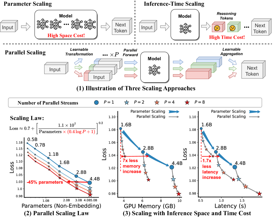
Figure 1: (1) Illustrations of our proposed parallel scaling (ParScale). (2) Parallel scaling laws for pre-training models on 42B tokens from Stack-V2 (Python subset). (3) Loss scaling curve with inference cost. Results are averaged from batch size $\in\{1,2,4,8\}$ and input + output tokens $\in\{128,256,512,1024\}$.

1 Introduction

Recent years have witnessed the rapid scaling of large language models (LLMs) (Brown et al., 2020; OpenAI, 2023; Llama Team, 2024; Qwen Team, 2025b) to narrow the gap towards Artificial General Intelligence (AGI). Mainstream efforts focus on parameter scaling (Kaplan et al., 2020), a practice that requires substantial space overhead. For example, DeepSeek-V3 (Liu et al., 2024a) scales the model size up to 672B parameters, which imposes prohibitive memory requirements for edge deployment. More recently, researchers have explored inference-time scaling (OpenAI, 2024) to enhance the reasoning capability by scaling the number of generated reasoning tokens. However, inference-time scaling is limited to certain scenarios and necessitates specialized training data (DeepSeek-AI, 2025; Qin et al., 2024), and typically imposes significant time costs. For example, Chen et al. (2024b) find that the most powerful models can generate up to 900 reasoning tokens for trivial problems like “2+3=?”. This motivates the question: Is there a universal and efficient scaling approach that avoids excessive space and time costs?

We draw inspiration from classifier-free guidance (CFG) (Ho & Salimans, 2022), a widely used trick during the inference phase of diffusion models (Ho et al., 2020), with similar concepts also developed in the NLP community (Sanchez et al., 2024; Li et al., 2023). Unlike traditional methods that use a single forward pass, CFG utilizes two forward passes during inference: it first performs a normal forward pass to obtain the first stream of output, then perturbs the input (e.g., by discarding conditions in the input) to get a second stream of output. The two streams are aggregated based on predetermined contrastive rules, yielding superior performance over single-pass outputs. Despite its widespread use, the theoretical guarantee of CFG remains an open question. In this paper, we hypothesize that the effectiveness of CFG lies in its double computation. We further propose the following hypothesis:

Hypothesis 1.

Scaling parallel computation (while maintaining the nearly constant parameters) enhances the model’s capability, with similar effects as scaling parameters.

We propose a proof-of-concept scaling approach called parallel scaling (ParScale) to validate this hypothesis on language models. The core idea is to increase the number of parallel streams while making the input transformation and output aggregation learnable. We propose appending $P$ different learnable prefixes to the input and feeding them in parallel into the model. These $P$ outputs are then aggregated into a single output using a dynamic weighted sum, as shown in Figure 1(1). This method efficiently scales parallel computation during both training and inference time by recycling existing parameters, which applies to various training algorithms, data, and tasks.

Our preliminary theoretical analysis suggests that the loss of ParScale may follow a power law similar to the Chinchilla scaling law (Hoffmann et al., 2022). We then carry out large-scale pre-training experiments on the Stack-V2 (Lozhkov et al., 2024) and Pile (Gao et al., 2021) corpus, by ranging $P$ from 1 to 8 and model parameters from 500M to 4.4B. We use the results to fit a new parallel scaling law that generalizes the Chinchilla scaling law, as depicted in Figure 1(2). It shows that parallelizing into P streams equates to scaling the model parameters by $\bm{\mathcal{O}(\log P)}$. Results on comprehensive tasks corroborate this conclusion. Unlike parameter scaling, ParScale introduces negligible parameters and increases only a little space overhead. It also leverages GPU-friendly parallel computation, shifting the memory bottleneck in LLM decoding to a computational bottleneck and, therefore, does not notably increase latency. For example, for a 1.6B model, when scaling to $P=8$ using ParScale, it uses 22$\times$ less memory increase and 6$\times$ less latency increase compared to parameter scaling that achieves the same model capacity (batch size = 1, detailed in Section 3.3). Figure 1(3) illustrates that ParScale offers superior inference efficiency.

Furthermore, we show that the high training cost of ParScale can be reduced by a two-stage approach: the first stage employs traditional training with most of the training data, and ParScale is applied only in the second stage with a small number of tokens. Based on this, we train 1.8B models with various $P$ and scale the training data to 1T tokens. The results of 21 downstream benchmarks indicate the efficacy of this strategy. For example, when scaling to $P=8$, it yields a 34% relative improvement for GSM8K and 23% relative improvement for MMLU using exactly the same training data. We also implement ParScale on an off-the-shelf model, Qwen-2.5 (Qwen Team, 2024), and demonstrate that ParScale is effective in both full and parameter-efficient fine-tuning settings. This also shows the viability of dynamic parallel scaling, which allows flexible adjustment of $P$ during deployment while freezing the backbone weights, to fit different application scenerios.

Table 1: Comparisons of mainstream LLM scaling strategies. We subdivide parameter scaling into traditional Dense Scaling and Mixture-of-Expert (MoE) Scaling (Fedus et al., 2022) for comparison. Inference-Time Scaling: Enhancing the reasoning ability through large-scale reinforcement learning (RL) to scale reasoning tokens during inference.

Method	Inference Time	Inference Space	Training Cost	Specialized Strategy
Dense Scaling	Moderate	High	Pre-training only	No
MoE Scaling	Low	High	Pre-training only	Load balancing
Inference-Time Scaling	High	Moderate	Post-training	RL / reward data
Parallel Scaling	Moderate	Moderate	Pre- or Post-training	No

Table 1 compares ParScale with other mainstream scaling strategies. Beyond introducing an efficient scaling approach for language models, our research also tries to address a more fundamental question in machine learning: Is a model’s capacity determined by the parameters or by the computation, and what is their individual contribution? Traditional machine learning models typically scale both parameters and computation simultaneously, making it difficult to determine their contribution ratio. The ParScale and the fitted parallel scaling law may offer a novel and quantitative perspective on this problem.

We posit that large computing can foster the emergence of large intelligence. We hope our work can inspire more ways to scaling computing towards AGI and provide insights for other areas of machine learning. Our key findings in this paper can be summarized as follows:

• Scaling $P$ times of parallel computation is similar to scaling parameters by a ratio of $\mathcal{O}(\log P)$, and larger models reap greater benefits from ParScale.

• Reasoning-intensive tasks (e.g., coding or math) benefit more from ParScale, which suggests that scaling computation can effectively push the boundary of reasoning.

• ParScale offers superior inference efficiency compared to parameter scaling due to the effective use of memory, particularly suitable for low-resource edge deployment.

• The training cost of ParScale can be significantly alleviated through a two-stage training strategy.

• ParScale remains effective with frozen main parameters for different $P$. This illustrates the potential of dynamic parallel scaling: switching $P$ to dynamically adapt model capabilities during inference.

Our code and 67 trained model checkpoints are publicly available at https://github.com/QwenLM/ParScale and https://huggingface.co/ParScale.

2 Background and Methodology

Classifier-Free Guidance (CFG)

CFG (Ho & Salimans, 2022) has become a de facto inference-time trick in diffusion models (Ho et al., 2020), with similar concepts also developed in NLP (Sanchez et al., 2024; Li et al., 2023). At a high level, these lines of work can be summarized as follows: given an input $x\in\mathbb{R}^{d_{i}}$ and a trained model $f_{\theta}:\mathbb{R}^{d_{i}}\rightarrow\mathbb{R}^{d_{o}}$, where $\theta$ is the parameter and $d_{i},d_{o}$ are dimensions, we transform $x$ into a “bad” version $x^{\prime}$ based on some heuristic rules (e.g., removing conditions), obtaining two parallel outputs $f_{\theta}(x)$ and $f_{\theta}(x^{\prime})$. The final output $g_{\theta}(x)$ is aggregated based on the following rule:

$$g_{\theta}(x)=f_{\theta}(x)+w\left(f_{\theta}(x)-f_{\theta}(x^{\prime})\right).$$ (1)

Here, $w>0$ is a pre-set hyperparameter. Intuitively, Equation 1 can be seen as starting from a “good” prediction and moving $w$ steps in the direction away from a “bad” prediction. Existing research shows that $g_{\theta}(x)$ can perform better than the vanilla $f_{\theta}(x)$ in practice (Saharia et al., 2022).

Motivation

In Equation 1, $x^{\prime}$ is simply a degraded version of $x$, suggesting that $g_{\theta}(x)$ does not gain more useful information than $f_{\theta}(x)$. This raises the question: why is $\bm{f_{\theta}(x)}$ unable to learn the capability of $\bm{g_{\theta}(x)}$ during training, despite both having the same parameters? We hypothesize that the fundamental reason lies in $g_{\theta}(x)$ having twice the computation as $f_{\theta}(x)$. This inspires us to further expand Equation 1 into the following form:

$$g_{\theta}(x)=w_{1}f_{\theta}(x_{1})+w_{2}f_{\theta}(x_{2})+\cdots+w_{P}f_{\theta}(x_{P}),$$ (2)

where $P$ denotes the number of parallel streams. $x_{1},\cdots,x_{P}$ are $P$ distinct transformations of $x$, and $w_{1},\cdots,w_{P}$ are aggregation weights. We term Equation 2 as a parallel scaling (ParScale) of the model $f_{\theta}$ with $P$ streams. This scaling strategy does not require changing the structure of $f_{\theta}$ and training data. In this paper, we focus on Transformer language models (Vaswani et al., 2017; Brown et al., 2020), and regard the stacked Transformer layers as $f_{\theta}(\cdot)$.

Implementation Details and Pivot Experiments

We apply Equation 2 in both training and inference time, and perform a series of pivot experiments to determine the best input transformation and output aggregation strategies (refer to Appendix A). The findings revealed that variations in these strategies minimally affect model performance; the significant factor is the number of computations (i.e., $\bm{P}$). Finally, for input transformation, we employ prefix tuning (Li & Liang, 2021) as the input transformation, which is equivalent to using different KV-caches to distinguish different streams. For output aggregation, we employ a dynamic weighted average approach, utilizing an MLP to convert outputs from multiple streams into aggregation weights. This increases about 0.2% additional parameters for each stream.

3 Parallel Scaling Law

This section focuses on the in-depth comparison of scaling parallel computation with scaling parameters. In Section 3.1, we theoretically demonstrate that parallel scaling is equivalent to increasing parameters by a certain amount. In Section 3.2, we validate this with a practical scaling law through large-scale experiments. Finally, in Section 3.3, we analyze latency and memory usage during inference to show that parallel scaling is more efficient.

3.1 Theoretical Analysis: Can ParScale Achieve Similar Effects as Parameter Scaling?

From another perspective, ParScale can be seen as an ensemble of multiple different next token predictions, despite the ensemble components sharing most of the parameters. Existing theory in literature finds that the ensembling performance depends on the diversity of different components (Breiman, 2001; Lobacheva et al., 2020b). In this section, we further validate this finding by theoretically proposing a new scaling law that generalizes existing language model scaling laws, and demonstrate that ParScale can achieve similar effects as parameter scaling.

We consider a special case that $w_{1}=w_{2}=\cdots=\nicefrac{{1}}{{P}}$ to simplify our analysis. This is a degraded version of ParScale, therefore, we can expect that the full version of ParScale is at least not worse than the theoretical results we can obtain (See Appendix A for further numeric comparison). Let $\hat{p}_{i}(\cdot\mid x)=f_{\theta}(x_{i})$ denote the next token distribution for the input sequence $x$ predicted by the $i$-th stream. Based on Equation 2, the final prediction $\hat{p}(\cdot\mid x)=g_{\theta}(x)$ is the average across $\hat{p}_{i}$, i.e., $\hat{p}(\cdot\mid x)=\nicefrac{{1}}{{P}}\sum_{i}\hat{p}_{i}(\cdot\mid x)$. Chinchilla (Hoffmann et al., 2022) proposes that the loss $\mathcal{L}$ of a language model with $N$ parameters is a function of $N$ after convergence. We assume the prediction of each stream adheres to the Chinchilla scaling law, as follows:

Lemma 3.1 (Chinchilla Scaling Law (Hoffmann et al., 2022)).

The language model cross-entropy loss $\mathcal{L}_{i}$ for the $i$-th stream prediction (with $N$ parameters) when convergence is:

$$\mathcal{L}_{i}=\left(\frac{A}{N}\right)^{\alpha}+E,\quad 1\leq i\leq P,$$ (3)

where $\{A,E,\alpha\}$ are some positive constants. $E$ is the entropy of natural text, and $N$ is the number of parameters.

Based on Lemma 3.1, we theoretically derive that after aggregating $P$ streams, the prediction follows a new type of scaling law, as follows:

Proposition 1 (Theoretical Formula for Parallel Scaling Law).

The loss $\mathcal{L}$ for ParScale (with $P$ streams and $N$ parameters) is

$$\mathcal{L}=\left(\frac{A}{N\cdot{P^{\nicefrac{{1}}{{\alpha}}}\cdot\textsc{Diversity}}}\right)^{\alpha}+E.$$ (4)

We define Diversity as:

$$\textsc{Diversity}=\left[(P-1)\rho+1\right]^{-\nicefrac{{1}}{{\alpha}}},$$

where $\rho$ is the correlation coefficient between random variables $\Delta p_{i}$ and $\Delta p_{j}$ ($i\neq j$), and $\Delta p_{i}$ is the relative residuals for the $i$-th stream prediction, i.e., $\Delta p_{i}=\nicefrac{{[\hat{p}_{i}(y\mid x)-p(y\mid x)]}}{{p(y\mid x)}}$. $p(y\mid x)$ is the real next token probability.

Proof for Proposition 1 is elaborated in Appendix B. From it, we can observe two key insights:

1. When $\rho=1$, predictions across different streams are identical, at which point we can validate that Equation 4 degenerates into Equation 3. Random initialization on a small number of parameters introduced (i.e., prefix embeddings) is sufficient to avoid this situation in our experiments, likely due to the impact being magnified by the extensive computation of LLMs.

2. When $\rho\neq 1$, $\mathcal{L}$ is inversely correlated to $P$. Notably, when $\rho=0$, residuals are independent between streams and the training loss exhibits a power-law relationship with $P$ (i.e., $\mathcal{L}\propto P^{-1}$). This aligns with findings in Lobacheva et al. (2020b). When $\rho$ is negative, the loss can further decrease and approach zero. This somewhat demystifies the effectiveness of CFG: by widening the gap between “good” input $x$ and “bad” input $x^{\prime}$, we force the model to “think” from two distinct perspectives, which can increase the diversity between the two outputs.

Despite the difficulty in further modeling $\rho$, Proposition 1 suggests that scaling $\bm{P}$ times of parallel computation is equivalent to scaling the model parameter count, by a factor of $\bm{(P^{\nicefrac{{1}}{{\alpha}}}\cdot}$Diversity$\bm{)}$. This motivates us to go further, by empirically fitting a practical parallel scaling law to validate 1.

3.2 Practical Parallel Scaling Laws

Experiment Setup

To fit a parallel scaling law in practice, we pre-train Transformer language models with the Qwen-2.5 dense architecture and tokenizer (Qwen Team, 2024) from scratch on the open-source corpus. Models have up to 4.7 billion parameters (with 4.4B non-embedding parameters) and 8 parallel streams. We primarily focus on the relationship between parallel scaling and parameter scaling. Therefore, we fix the training data size at 42 billion tokens without data repeat. We introduce the results for more training tokens in the next section, and leave the impact of data scale on our scaling laws for future work. We use a batch size of 1024 and a sequence length of 2048, resulting in 20K training steps. For models with $P>1$, we incorporate prefix embeddings and aggregation weight, as introduced in Appendix A. No additional parameters are included for $P=1$ models to maintain alignment with existing architectures. We report the last step training loss using exponential moving average, with a smoothing weight of 0.95. Other hyperparameters follow existing works (Muennighoff et al., 2023) and are detailed in Appendix C.

Our pre-training is conducted on two widely utilized datasets: Stack-V2 (Python subset) (Lozhkov et al., 2024) and Pile (Gao et al., 2021). Pile serves as a general corpus aimed at enhancing common sense and memorization skills, while Stack-V2 focuses on code comprehension and reasoning skills. Analyzing ParScale across these contexts can assess how parameters and computations contribute to different skills.

Parametric Fitting

We plot the results in Figure 2, where each point represents the loss of a training run, detailed in Appendix F. We observe that increasing $P$ yields benefits following a logarithmic trend. Similar gains are seen when raising $P$ from 1 to 2, 2 to 4, and 4 to 8. Thus, we preliminarily try the following form:

$$\mathcal{L}=\left(\frac{A}{N\cdot(k\log P+1)}\right)^{\alpha}+E,$$ (5)

where we assume that $P^{\nicefrac{{1}}{{\alpha}}}\cdot\textsc{Diversity}=k\log P+1$ in Equation 4 based on the finding of the logarithmic trend. $(A,k,\alpha,E)$ are parameters to fit, and we use the natural logarithm (base $e$). We follow the fitting procedure from Hoffmann et al. (2022); Muennighoff et al. (2023), detailed in Appendix E.

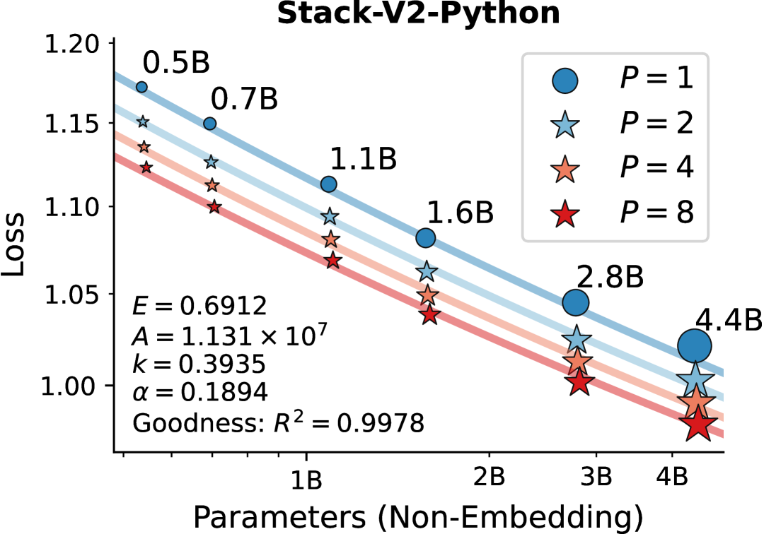
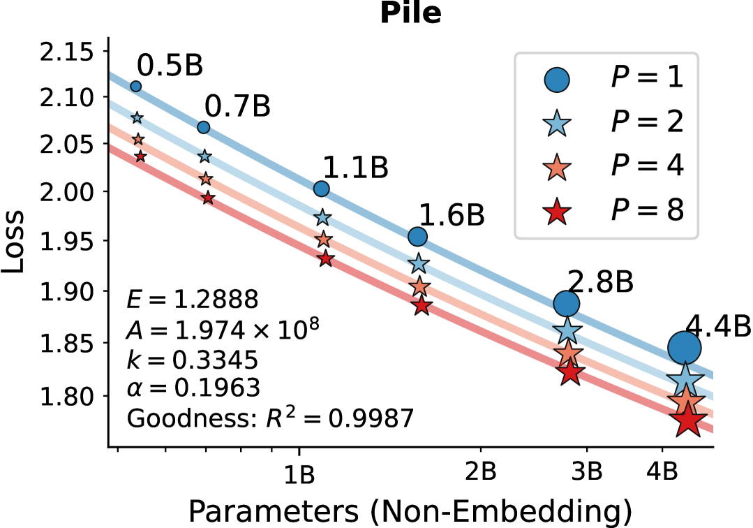
Figure 2: Loss of LLMs scaled on parameters and number of parallel streams $P$ trained on 42B tokens. Each point depicts the loss from a training run. The fitted scaling law curve from Equation 5 is displayed, with annotated fitted parameters $(E,A,k,\alpha)$ and the goodness of fit $R^{2}$.

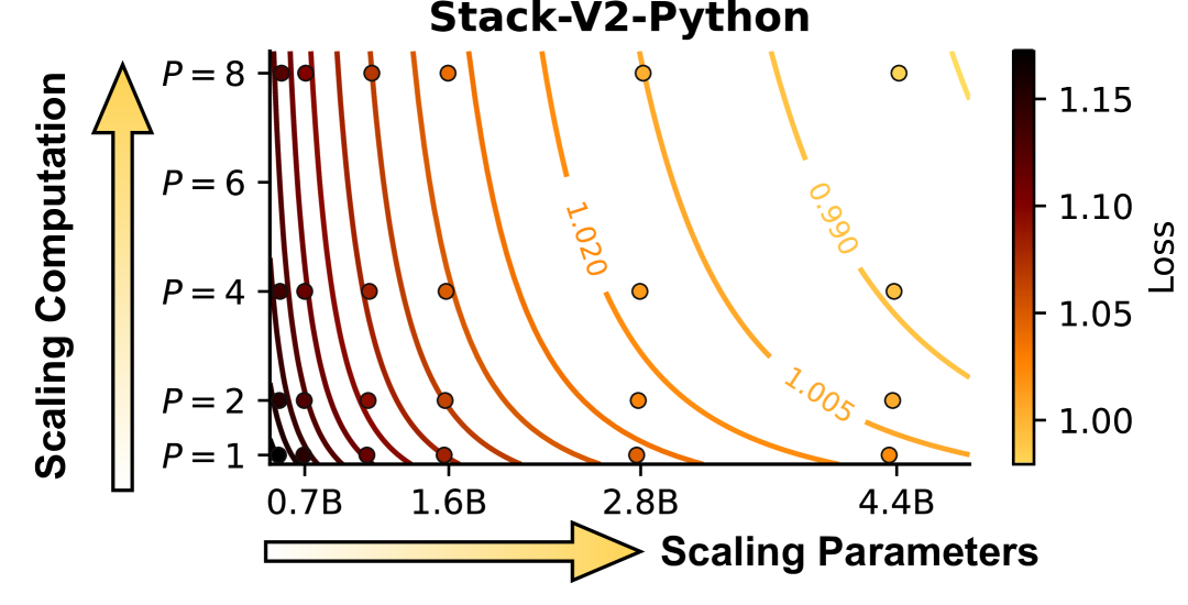
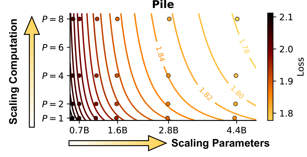
Figure 3: Predicted loss contours for ParScale. Each contour line indicates a combination of (parameter, $P$) with similar performance.

Figure 2 illustrates the parallel scaling law fitted for two training datasets. It shows a high goodness of fit ($R^{2}$ up to $0.998$), validating the effectiveness of Equation 5. Notably, we can observe that the $k$ value for Stack-V2 (0.39) is higher than for Pile (0.33). Recall that $k$ reflects the benefits of increased parallel computation. Since Stack-V2 emphasizes coding and reasoning abilities while Pile emphasizes memorization capacity, we propose an intuitive conjecture that model parameters mainly impact the memorization skills, while computation mainly impacts the reasoning skills. This aligns with recent findings on inference-time scaling (Geiping et al., 2025). Unlike those studies, we further quantitatively assess the ratio of contribution to model performance between parameters and computation through our proposed scaling laws.

Recall that Equation 5 implies scaling $P$ equates to increasing parameters by $\mathcal{O}(N\log P)$. It suggests that models with more parameters benefit more from ParScale. Figure 3 more intuitively displays the influence of computation and parameters on model capacity. As model parameters increase, the loss contours flatten, showing greater benefits from increasing computation.

Table 2: Average performance (%) on two code generation tasks, HumanEval(+) and MBPP(+), after pre-training on the Stack-V2-Python dataset.

$N$	0.5B	0.7B	1.1B	1.6B	2.8B	4.4B
$P=1$	26.7	28.4	31.6	33.9	36.9	39.2
$P=2$	30.3	32.4	33.6	37.4	39.4	42.6
$P=4$	30.1	32.5	34.1	37.6	40.7	42.6
$P=8$	32.3	34.0	37.2	39.1	42.1	45.4

Table 3: Average performance (%) on six general lm-evaluation-harness tasks after pre-training on the Pile dataset.

$N$	0.5B	0.7B	1.1B	1.6B	2.8B	4.4B
$P=1$	49.1	50.6	52.1	53.1	55.2	57.2
$P=2$	49.9	51.0	52.4	54.4	57.0	58.5
$P=4$	50.6	51.8	53.3	55.0	57.8	59.1
$P=8$	50.7	51.8	54.2	55.7	58.1	59.6

Downstream Performance

Tables 3 and 3 illustrate the average performance on downstream tasks (coding tasks for Stack-V2-Python and general tasks for Pile) after pre-training, with comprehensive results in Appendix G. It shows that increasing the number of parallel streams $P$ consistently boosts performance, which confirms that ParScale is able to enhance the model capabilities and similar to scale the parameters. Notably, ParScale offers more substantial improvements for coding tasks compared to general tasks. For example, as shown in Table 3, the coding ability of the 1.6B model for $P=8$ aligns with the 4.4B model, while Table 3 indicates that such setting performs comparably to the 2.8B model on general tasks that focusing on common-sense memorization. These findings affirm our previous hypothesis that the number of parameters impacts the memorization capacity, while computation impacts the reasoning capacity.

3.3 Inference Cost Analysis

We further compare the inference efficiency between parallel scaling and parameter scaling at equivalent performance levels. Although some work uses FLOPS to measure the inference cost (Hoffmann et al., 2022; Sardana et al., 2024), we argue that this is not an ideal metric. Most Transformer operations are bottlenecked by memory access rather than computation during the decoding stage (Ivanov et al., 2021). Some work (such as flash attention (Dao et al., 2022)) incurs more FLOPS but achieves lower latency by reducing memory access. Therefore, we use memory and latency to measure the inference cost, based on the llm-analysis framework (Li, 2023). Memory determines the minimum hardware requirements, while latency measures the time overhead from input to output.

We analyze the inference cost across various inference batch sizes. It is worth mentioning that all models in our experiments feature the same number of layers, differing only in parameter width and parallel streams (detailed in Appendix C). This enables a more fair comparison of the efficiencies.

Space Cost

LABEL:fig:cost_memory_1, LABEL:fig:cost_memory_2, LABEL:fig:cost_memory_4 and LABEL:fig:cost_memory_8 compare the inference memory usage of two scaling strategies, where we utilize loss on Stack-V2-Python as an indicator for model capacity. It shows that ParScale only marginally increases memory usage, even with larger batch sizes. This is because ParScale introduces negligible amounts of additional parameters (i.e., prefix tokens and aggregation weights, about 0.2% parameters per stream) and increases KV cache size (expanded by $P$ times with $P$ streams), which generally occupies far less GPU memory than model parameters. As the input batch size increases, the KV cache size also grows; however, ParScale continues to demonstrate significantly better memory efficiency compared to parameter scaling. This suggests that ParScale maximizes the utility of memory through parameter reusing, while parameter scaling employs limited computation per parameter and cannot fully exploit computation resources.

Time Cost

LABEL:fig:cost_latency_1, LABEL:fig:cost_latency_2, LABEL:fig:cost_latency_4 and LABEL:fig:cost_latency_8 compare the inference time of two scaling strategies. It shows that ParScale adds minimal latency at smaller batch sizes since the memory bottlenect is converted tothe computation bottleneck. Given that parallel computation introduced by ParScale is friendly to GPUs, it will not significantly raise latency. As batch sizes increase, decoding shifts from a memory to a computation bottleneck, resulting in higher costs for ParScale, but it remains more efficient than parameter scaling up to a batch size of 8.

The above analysis indicates that ParScale is ideal for low-resource edge devices like smartphones, smart cars, and robots, where queries are typically few and batch sizes are small. Given limited memory resources in these environments, ParScale effectively utilizes memory and latency advantages at small batch sizes. When batch size is 1, for a 1.6B model and scaling to P = 8 using ParScale, it uses 22$\times$ less memory increase and 6$\times$ less latency increase compared to parameter scaling that achieves the same performance. We anticipate that the future LLMs will gradually shift from centralized server deployments to edge deployments with the popularization of artificial intelligence. This suggests the promising potential of ParScale in the future.

4 Scaling Training Data

Due to our limited budget, our previous experiments on scaling laws focus on pre-training with 42 billion tokens. In this section, we will train a 1.8B model (with 1.6B non-embedding parameters) and scale the training data to 1T tokens, to investigate whether ParScale is effective for production-level training. We also apply ParScale to an off-the-shelf model, Qwen-2.5 (Qwen Team, 2024) (which is pre-trained on 18T tokens), under two settings: continual pre-training and parameter-efficient fine-tuning (PEFT).

4.1 Two-Stage Pretraining

While ParScale is efficient for the inference stage (as we discuss in Section 3.3), it still introduces about $P$ times of floating-point operations and significantly increases overhead in the computation-intensive training processes. To address this limitation, we propose a two-stage strategy: in the first stage, we use traditional pre-training methods with 1 trillion tokens; in the second stage, we conduct ParScale training with 20 billion tokens. Since the second stage accounts for only 2% of the first stage, this strategy can greatly reduce training costs. This two-stage strategy is similar to long-context fine-tuning (Ding et al., 2024), which also positions the more resource-intensive phase at the end. In this section, we will examine the effectiveness of this strategy.

Setup

We follow Allal et al. (2025) and use the Warmup Stable Decay (WSD) learning rate schedule (Hu et al., 2024; Zhai et al., 2021). In the first stage, employing a 2K step warm-up followed by a fixed learning rate of 3e-4. In the second stage, the learning rate is annealed from 3e-4 to 1e-5. The rest of the hyperparameters remain consistent with the previous experiments (see Appendix C).

In the first phase, we do not employ the ParScale technique. We refer to the recipe proposed by Allal et al. (2025) to construct our training data, which consists of 370B general data, 80B mathematics data, and 50B code data. We train the model for two epochs to consume 1T tokens. Among the general text, there are 345B from FineWeb-Edu (Penedo et al., 2024) and 28B from Cosmopedia 2 (Ben Allal et al., 2024); the mathematics data includes 80B from FineMath (Allal et al., 2025); and the code data comprises 47B from Stack-V2-Python and 4B from Stack-Python-Edu.

In the second phase, we use the trained model from the first phase as the backbone and introduce additional parameters from ParScale, which are randomly initialized using a standard deviation of 0.02 (based on the initialization of Qwen-2.5). Following (Allal et al., 2025), in this phase, we increase the proportion of mathematics and code data, finally including a total of 7B general text data, 7B mathematics data, and 7B Stack-Python-Edu data.

Table 4: Performance comparison of the 1.8B models after training on 1T tokens from scratch using the two-stage strategy. We incorporate recent strong baselines (less than 2B parameters) as a comparison to validate that our $P=1$ baseline is well-trained. The best performance and its comparable performance (within 0.5%) is bolded. Appendix G elaborates the evaluation details. @1: Pass@1. @10: Pass@10.

	Tokens	Data	Average				General
			General	Math	Code		MMLU	WinoGrande	Hellaswag	OBQA	PiQA	ARC
gemma-3-1B	2T	Private	53.4	1.9	14.9		26.4	61.4	63.0	37.8	75.6	56.2
Llama-3.2-1B	15T	Private	54.8	4.7	30.1		30.8	62.1	65.7	39.2	75.9	55.3
Qwen2.5-1.5B	18T	Private	63.6	52.3	55.8		61.0	65.6	68.0	42.6	76.6	67.9
SmolLM-1.7B	1T	Public	57.0	6.0	37.9		29.7	61.8	67.3	42.8	77.3	63.3
SmolLM2-1.7B	12T	Public	63.3	24.3	41.6		50.1	68.2	73.1	42.6	78.3	67.3
Baseline ($P=1$)	1T	Public	56.0	25.5	45.6		28.5	61.9	65.0	40.6	75.2	64.8
ParScale ($P=2$)	1T	Public	56.2	27.1	47.4		29.0	62.4	64.7	42.0	74.9	64.3
ParScale ($P=4$)	1T	Public	57.2	30.0	48.6		30.0	63.4	65.9	42.0	75.6	66.3
ParScale ($P=8$)	1T	Public	58.6	32.8	49.9		35.1	64.9	67.0	42.6	76.1	66.0

	Tokens	Data	Math				Code
			GSM8K	GSM8K	Minerva		HumanEval			HumanEval+			MBPP			MBPP+
				+CoT	Math		@1	@10		@1	@10		@1	@10		@1	@10
gemma-3-1B	2T	Private	1.8	2.3	1.5		6.7	15.9		6.1	14.6		13.0	29.1		10.8	23.0
Llama-3.2-1B	15T	Private	5.1	7.2	1.8		16.5	27.4		14.0	25.0		33.1	54.5		27.0	43.4
Qwen2.5-1.5B	18T	Private	61.7	67.2	28.1		36.0	62.8		31.1	55.5		61.9	79.6		50.8	68.5
SmolLM-1.7B	1T	Public	6.4	8.3	3.2		20.1	35.4		15.9	32.3		40.7	66.4		34.7	57.4
SmolLM2-1.7B	12T	Public	30.4	30.8	11.8		23.8	44.5		18.9	37.8		45.2	68.5		36.0	57.9
Baseline ($P=1$)	1T	Public	28.7	35.9	12.0		26.8	44.5		20.7	38.4		51.6	75.9		43.9	62.7
ParScale ($P=2$)	1T	Public	32.6	35.6	13.0		26.2	50.0		20.1	42.1		52.9	77.0		45.0	65.6
ParScale ($P=4$)	1T	Public	34.7	40.8	14.5		27.4	47.6		23.8	43.9		55.3	77.0		47.1	66.7
ParScale ($P=8$)	1T	Public	38.4	43.7	16.4		28.7	50.6		24.4	44.5		56.3	79.1		48.1	67.2

Training Loss

Figure 11 intuitively demonstrates the loss curve during our two-stage training. We find that at the beginning of the second phase, the loss for $P>1$ initially exceed those for $P=1$ due to the introduction of randomly initialized parameters. However, after processing a small amount of data (0.0002T tokens), the model quickly adapts to these newly introduced parameters and remains stable thereafter. This proves that ParScale can take effect rapidly with just a little data. We can also find that in the later stages, ParScale yields similar logarithmic gains. This aligns with previous scaling law findings, suggesting that our earlier conclusions for from-scratch pre-training — parallelism with $P$ streams equates to a $\mathcal{O}(N\log(P))$ increase in parameters — also applies to continued pretraining. Additionally, larger $P$ (such as $P=8$) can gradually widen the gap compared to smaller $P$ values (such as $P=4$). This demonstrates that parallel scaling can also benefit from data scaling.

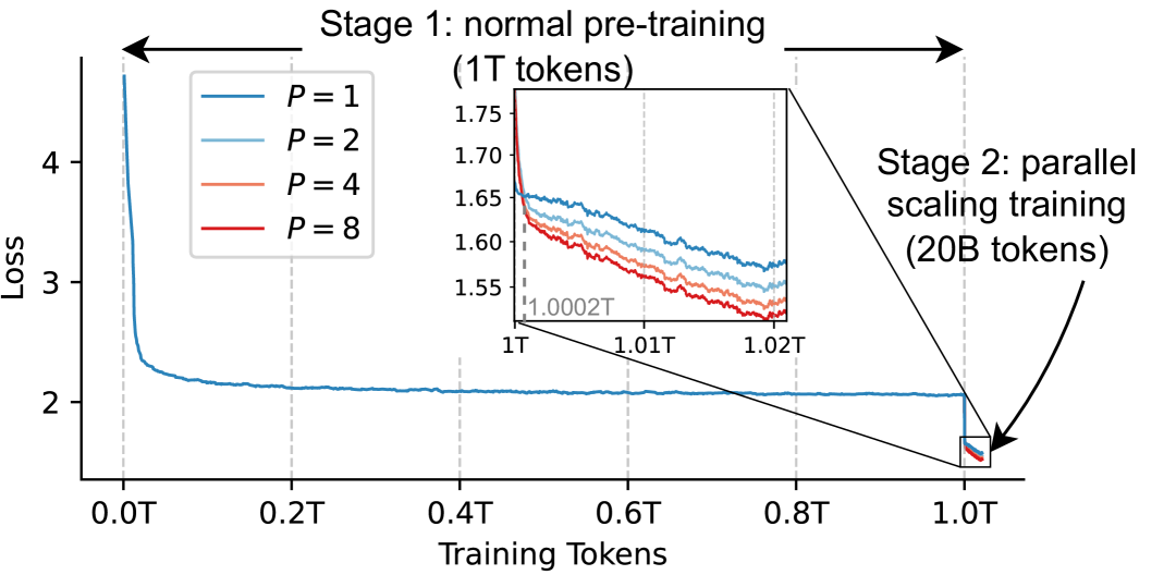
Figure 11: Loss for two-stage training, smoothing using an exponential moving average with a weight of 0.95.

Table 5: Comparison of the performance of different Instruct models, where the few-shot examples are treated as a multi-turn conversation.

	IFEval	MMLU	GSM8K
	0-shot	5-shot	4-shot
SmolLM-1.7B-Inst	16.3	28.4	2.0
Baseline-Inst ($P=1$)	54.1	34.2	50.3
ParScale-Inst ($P=2$)	55.8	35.1	55.3
ParScale-Inst ($P=4$)	58.4	38.2	54.8
ParScale-Inst ($P=8$)	59.5	41.7	56.1

Downstream Performance

In Table 4, we report the downstream performance of the model after finishing two-stage training, across 7 general tasks, 3 math tasks, and 8 coding tasks. It can be observed that with the increase of $P$, the performance presents an upward trend for most of the benchmarks, which validates the effectiveness of ParScale trained on the large dataset. Specifically, when $P$ increases from 1 to 8, ParScale improves by 2.6% on general tasks, and by 7.3% and 4.3% on math and code tasks, respectively. It achieves a 10% improvement (34% relative improvement) on GSM8K. This reaffirms that ParScale can more effectively address reasoning-intensive tasks. Moreover, in combination with CoT, it achieves about an 8% improvement on GSM8K, suggesting that parallel scaling can be used together with inference-time scaling to achieve better results. Compared to the SmolLM-1.7B model, which was also trained on 1T tokens, our $P=1$ baseline achieves comparable results on general tasks and significantly outperforms on math and code tasks. One explanation is that SmolLM training set focuses more on commonsense and world knowledge corpus, while lacking high-quality math and code data. This validates the effectiveness of our dataset construction and training strategy, and further enhances the credibility of our experimental results.

Instruction Tuning

We follow standard practice to post-train the base models, to explore whether ParScale can enhance performance during the post-training stage. We conducted instruction tuning on four checkpoints ($P\in\{1,2,4,8\}$) from the previous pre-training step, increasing the sequence length from 2048 to 8192 and the RoPE base from 10,000 to 100,000, while keeping other hyperparameters constant. We used 1 million SmolTalk (Allal et al., 2025) as the instruction tuning data and trained for 2 epochs. We refer to these instruction models as ParScale-Inst.

The experimental results in Section 4.1 show that when $P$ increases from 1 to 8, our method achieves a 5% improvement on the instruction-following benchmark IFEval, along with substantial gains in the general task MMLU and the reasoning task GSM8K. This demonstrates that the proposed ParScale performs effectively during the post-training phase.

4.2 Applying to the Off-the-Shelf Pre-Trained Model

We further investigate applying ParScale to off-the-shelf models under two settings: continual pre-training and parameter-efficient fine-tuning (PEFT). Specifically, we use Pile and Stack-V2 (Python) to continue pre-training the Qwen-2.5 (3B) model. The training settings remain consistent with Appendix C, with the only difference being that we initialize with Qwen2.5-3B weights and adjust the RoPE base to the preset 1,000,000.

Continual Pre-Training

LABEL:fig:qwen_pile and LABEL:fig:qwen_stack illustrates the training loss after continuous pre-training on Stack-V2 (Python) and Pile. Notably, Qwen2.5 has already been pre-trained on 18T of data, which possibly have significant overlap with both Pile and Stack-V2. This demonstrates that improvements can still be achieved even with a thoroughly trained foundation model and commonly used training datasets.

Parameter-Efficient Fine-Tuning

We further utilize PEFT to fine-tune the introduced parameters while freezing the backbone weights. LABEL:fig:qwen_peft shows that this strategy can still significantly improve downstream code generation performance. Moreover, this demonstrates the promising prospects of dynamic parallel scaling: we can deploy the same backbone and flexibly switch between different numbers of parallel streams in various scenarios (e.g., high throughput and low throughput), which enables quick transitions between different levels of model capacities.

5 Related Work

Beyond language modeling, our work can be connected to various machine learning domains. First, scaling computation while maintaining parameters is also the core idea of inference-time scaling. Second, as previously mentioned, ParScale can be viewed as a dynamic and scalable classifier-free guidance. Third, our method can be seen as a special case of model ensemble. Lastly, the parallel scaling law we explore is a generalization of the existing language model scaling laws.

Inference-Time Scaling

The notable successes of reasoning models, such as GPT-o1 (OpenAI, 2024), DeepSeek-R1 (DeepSeek-AI, 2025), QwQ (Qwen Team, 2025a), and Kimi k1.5 (Kimi Team, 2025) have heightened interest in inference-time scaling. These lines of work (Wei et al., 2022; Madaan et al., 2023; Zhou et al., 2023a) focus on scaling serial computation to increase the length of the chain-of-thought (Wei et al., 2022). Despite impressiveness, it results in inefficient inference and sometimes exhibits overthinking problems (Chen et al., 2024b; Sui et al., 2025).

Other lines of approaches focus on scaling parallel computation. Early methods such as beam search (Wiseman & Rush, 2016), self-consistency (Wang et al., 2023b), and majority voting (Chen et al., 2024a) require no additional training. We also provide an experimental comparison with Beam Search in Appendix H, which shows the importance of scaling parallel computing during the training stage. Recently, the proposal-verifier paradigm has gained attention, by employing a trained verifier to select from multiple parallel outputs (Brown et al., 2024; Wu et al., 2025; Zhang et al., 2024b). However, these methods are limited to certain application scenarios (i.e., generation tasks) and specialized training data (i.e., reward signals).

More recently, Geiping et al. (2025) introduce training LLMs to reason within the latent space and scale sequential computation, applicable to any application scenarios without needing specialized datasets. However, this method demands significant serial computation scaling (e.g., 64 times the looping) and invasive model modifications, necessitating training from scratch and complicating integration with existing trained LLMs.

Classifier-Free Guidance

Classifier-Free Guidance (CFG) stems from Classifier Guided Diffusion (Dhariwal & Nichol, 2021), which uses an additional classifier to guide image generation using diffusion models (Ho et al., 2020). By using the generation model itself as a classifier, CFG (Ho & Salimans, 2022) further eliminates dependency on the classifier and leverage two forward passes. Similar concepts have emerged in NLP, such as Coherence Boosting (Malkin et al., 2022), PREADD (Pei et al., 2023), Context-Aware Decoding (Shi et al., 2024), and Contrastive Decoding (Li et al., 2023). Recently, Sanchez et al. (2024) proposed transferring CFG to language models. However, due to constraints of human-designed heuristic rules, these techniques cannot leverage the power of training-time scaling (Kaplan et al., 2020) and the performance is limited.

Model Ensemble

Model ensemble is a classic research field in machine learning and is also employed in the context of LLMs (Chen et al., 2025). In traditional model ensembles, most ensemble components do not share parameters. Some recent work consider setups with partially shared parameters. For example, Monte Carlo dropout (Gal & Ghahramani, 2016) employs multiple different random dropouts during the inference phase, while BatchEnsemble (Wen et al., 2020; Tran et al., 2022) and LoRA ensemble (Wang et al., 2023a) use distinct low-rank matrix factorizations for model weights to differentiate different streams (we also experimented with this technique as input transformation in Appendix A). Weight sharing (Yang et al., 2021; Lan et al., 2019) is another line of work, where some weights of a model are shared across different components and participate in multiple computations. However, these works have not explored the scaling law of parallel computation from the perspective of model capacity. As we discuss in Appendix A, we find that the specific differentiation technique had a minimal impact, and the key factor is the scaling in parallel computation.

Scaling Laws for Language Models

Many researchers explore the predictable relationships between LLM training performance and various factors under different settings, such as the number of parameters and data (Hestness et al., 2017; Kaplan et al., 2020; Hoffmann et al., 2022; DeepSeek-AI, 2024; Frantar et al., 2024), data repetition cycles (Muennighoff et al., 2023; Hernandez et al., 2022), data mixing (Ye et al., 2025; Que et al., 2024), and fine-tuning (Zhang et al., 2024a). By extending the predictive empirical scaling laws developed from smaller models to larger models, we can significantly reduce exploration costs. Recently, some studies have investigated the scaling effects during inference (Sardana et al., 2024), noting a log-linear relationship between sampling number and performance (Brown et al., 2024; Snell et al., 2025). But they are limited to certain application scenarios. Our work extends the Chinchilla scaling law (Hoffmann et al., 2022) by introducing the intrinsic quantitative relationship between parallel scaling and parameter scaling. Existing literature has also identified a power-law relationship between the number of ensembles and loss in model ensemble scaling laws (Lobacheva et al., 2020a), which can be considered a special case of Proposition 1 when $\rho=0$.

6 Discussion and Future Work

Training Inference-Optimal Language Models

Chinchilla (Hoffmann et al., 2022) explored the scaling law to determine the training-optimal amounts for parameters and training data under a training FLOP budget. On the other hands, modern LLMs are increasingly interested on inference-optimal models. Some practitioners use much more data than the Chinchilla recommendation to train small models due to their high inference efficiency (Qwen Team, 2024; Allal et al., 2025; Sardana et al., 2024). Recent inference-time scaling efforts attempt to provide a computation-optimal strategy during the inference phase (Wu et al., 2025; Snell et al., 2025), but most rely on specific scenarios and datasets. Leveraging the proposed ParScale, determining how to allocate the number of parameters and parallel computation under various inference budgets (e.g., memory, latency, and batch size) to extend inference-optimal scaling laws (Sardana et al., 2024) is a promising direction.

Further Theoretical Analysis for Parallel Scaling Laws

One of our contributions is quantitatively computing the impact of parameters and computation on model capability. Although we present some theoretical results (Proposition 1), the challenge of directly modeling Diversity limits us to using extensive experiments to fit parallel scaling laws. Why the diversity is related to $\log P$, is there a growth rate that exceeds $\mathcal{O}(\log P)$, and whether there is a performance upper bound for $P\gg 8$, remain open questions.

Optimal Division Point of Two-Stage Strategy

Considering that ParScale is inefficient in the training phase, we introduced a two-stage strategy and found that LLMs can still learn to leverage parallel computation for better capacity with relatively few tokens. We currently employ a 1T vs. 20B tokens as the division point. Whether there is a more optimal division strategy and its trade-off with performance is also an interesting research direction.

Application to MoE Architecture

Similar to the method proposed by Geiping et al. (2025), ParScale is a computation-heavy (but more efficient) strategy. This is somewhat complementary to sparse MoE (Fedus et al., 2022; Shazeer et al., 2017), which is parameter-heavy. Considering that MoE is latency-friendly while ParScale is memory-friendly, exploring whether their combination can yield more efficient and high-performing models is worth investigating.

Application to Other Machine Learning Domains

Although we focus on language models, ParScale is a more general method that can be applied to any model architecture, training algorithm, and training data. Exploring ParScale in other areas and even proposing new scaling laws is also a promising direction for the future.

7 Conclusions

In this paper, we propose a new type of scaling strategy, ParScale, for training LLMs by reusing existing parameters for multiple times to scale the parallel computation. Our theoretical analysis and extensive experiments propose a parallel scaling law, showing that a model with $N$ parameters and $P\times$ parallel computation can be comparable to a model with $\mathcal{O}(N\log P)$ parameters. We scale the training data to 1T tokens to validate ParScale in the real-world practice based on the proposed two-stage strategy, and show that ParScale remains effective with frozen main parameters for different $P$. We also demonstrate that parallel scaling is more efficient than parameter scaling during the inference time, especially in low-resource edge scenarios. As artificial intelligence becomes increasingly widespread, we believe that future LLMs will progressively transition from centralized server deployments to edge deployments, and ParScale could emerge as a promising technique for these scenarios.

Appendix

Appendix A Implementation Details and Pivot Experiments

Input Transformation

We expect that the transformations applied to the input embedding $x$ can significantly influence the output, which avoids excessively similar outputs across different parallel streams. This can be achieved through the Soft Prompting technique (Lester et al., 2021). Specifically, Lester et al. (2021) introduced trainable continuous embeddings, known as soft prompts, which are appended to the original sequence of input word embeddings. Freezing the main network while only fine-tuning these soft prompts can be comparable to full fine-tuning. Building on this concept, prefix-tuning (Li & Liang, 2021) incorporates soft prompts into every attention layer of the Transformer model and appends them to the key and value vectors, showing superiority performance to soft prompts.

We utilize prefix-tuning to implement input transformation. To be specific, we first duplicate the input $x$ into $P$ parallel copies, distinguishing them with different prefixes in each attention layer. This can be implemented as using different KV caches for different streams. We found that randomly initializing the prefixes is sufficient to ensure diverse outputs across different streams. We also leverage the prefix reparameterization trick (Li & Liang, 2021; Han et al., 2024), which is theoretically proved effectiveness by Le et al. (2025).

As a comparison, we also compared using other parameter-efficient fine-tuning strategy for discriminating the input, including LoRA (Hu et al., 2022) and BitFit (Ben Zaken et al., 2022). Notably, LoRA has been also applied to the model ensemble scenario in the literature (Wang et al., 2023a), but only used in the fine-tuning setting while freezing the main parameters in their experiments.

Output Aggregation

We found that using dynamic aggregation weights performs better than static ones. Specifically, we concatenate each output together and use an MLP $h:\mathbb{R}^{d_{o}\times P}\rightarrow\mathbb{R}^{P}$ to convert it into a vector of length $P$ as aggregation weights. The process can be formalized as:

$$w_{1},\cdots,w_{P}\leftarrow\text{Softmax}\left(h\left(\text{Concat}[f_{\theta}(x_{1});\cdots;f_{\theta}(x_{P})]\right)\right),$$ (6)

where Softmax ensures aggregation weights are normalized. It can be seen as dynamically weighting different parallel streams during forward process for each token. We observed that, in the early stages of training, the model may assign nearly all weight to a few streams, leaving others with near-zero weights. It prevents the prefix parameters of these unlucky streams from receiving gradients and updates. This is similar to the load imbalance phenomenon in sparse MoE architectures (Fedus et al., 2022; Shazeer et al., 2017), where most tokens are sometimes assigned to a few experts. To address this, we apply label smoothing (Szegedy et al., 2016) to set a non-zero minimum for each weight, formulated as:

$$w_{i}\leftarrow w_{i}\times(1-\epsilon)+\frac{\epsilon}{P},$$ (7)

where $\epsilon$ denotes the smoothing parameter and we set it to $0.1$ in our experiments.

As a comparison, we also compare using Linear layer to aggregate different outputs and directly average the outputs.

Results

We trained a 0.5B model on Stack-V2-Python. Table 6 compares the impact of different strategies on final performance. For output aggregation, a dynamic weighted sum with label smoothing proved most effective. The differences between methods for input transformation were minor (around 0.1%), much less than the benefits obtained from changing $P$. Therefore, we opt for the simplest strategy, prefix tuning. Unlike LoRA and BitFit, it requires minimal changes to the model, only necessitating adjustments to the KV-cache.

Table 6: Comparisons of different strategies for input transformations and output aggregation.

$P$	Input Transformation	Output Aggregation	Loss $\downarrow$	Rel. Improvement $\uparrow$
1	-	-	1.1518	0.00%
2	Prefix (48 tokens)	Dynamic Weighted Sum ($\epsilon=0.1$)	1.1276	2.10%
2	Prefix (48 tokens)	Dynamic Weighted Sum ($\epsilon=0.0$)	1.1284	2.03%
2	Prefix (48 tokens)	Average	1.1288	2.00%
2	Prefix (48 tokens)	Linear Layer	1.1323	1.69%
2	Prefix (48 tokens)	Dynamic Weighted Sum ($\epsilon=0.1$)	1.1276	2.10%
2	Prefix (96 tokens)	Dynamic Weighted Sum ($\epsilon=0.1$)	1.1278	2.08%
2	LoRA ($r=2$)	Dynamic Weighted Sum ($\epsilon=0.1$)	1.1281	2.06%
2	Prefix (48 tokens) + LoRA ($r=2$)	Dynamic Weighted Sum ($\epsilon=0.1$)	1.1263	2.21%
2	Prefix (48 tokens) + LoRA ($r=2$) + BitFit	Dynamic Weighted Sum ($\epsilon=0.1$)	1.1263	2.21%
2	Prefix (48 tokens) + LoRA ($r=4$)	Dynamic Weighted Sum ($\epsilon=0.1$)	1.1260	2.24%
4	Prefix (48 tokens)	Dynamic Weighted Sum ($\epsilon=0.1$)	1.1145	3.24%
8	Prefix (48 tokens)	Dynamic Weighted Sum ($\epsilon=0.1$)	1.1019	4.33%

Appendix B Proof for Proposition 1

Proof.

We first decompose the individual loss $\mathcal{L}_{i}$. Based on the definition of language model loss, we have:

$$\mathcal{L}_{i} =\mathbb{E}_{x}\sum_{y\in\mathcal{V}}\left[-p(y\mid x)\log\hat{p}_{i}(y\mid x)\right]$$

$$=\mathbb{E}_{x}\sum_{y\in\mathcal{V}}-p(y\mid x)\log\left\{p(y\mid x)\times\left(1+\Delta p_{i}(y\mid x)\right)\right\}$$

$$=\underbrace{\mathbb{E}_{x}\sum_{y\in\mathcal{V}}\left[-p(y\mid x)\log p(y\mid x)\right]}_{\text{entropy of natural text}}+\underbrace{\mathbb{E}_{x}\sum_{y\in\mathcal{V}}-p(y\mid x)\log\left(1+\Delta p_{i}(y\mid x)\right)}_{\text{approximation error for the language model}},$$

where $\mathcal{V}$ is the vocabulary. In Chichilla scaling law, the entropy of natural text is $E$ and the approximation error is $(\nicefrac{{A}}{{N}})^{\alpha}$. Therefore, we have:

$$\mathbb{E}_{x}\sum_{y\in\mathcal{V}}-p(y\mid x)\log\left(1+\Delta p_{i}(y\mid x)\right)=\left(\frac{A}{N}\right)^{\alpha}.$$ (8)

Based on the Taylor series expansion, $\log(1+x)=x-\frac{x^{2}}{2}+\mathcal{O}(x^{3})$. Apply this expansion to Equation 8, we have:

$$\left(\frac{A}{N}\right)^{\alpha} =\mathbb{E}_{x}\sum_{y\in\mathcal{V}}-p(y\mid x)\left[\Delta p_{i}(y\mid x)-\frac{\Delta p_{i}(y\mid x)^{2}}{2}+\mathcal{O}\left(\Delta p_{i}(y\mid x)^{3}\right)\right]$$

$$=\mathbb{E}_{x}\left[\sum_{y\in\mathcal{V}}-\left(\hat{p}_{i}(y\mid x)-p(y\mid x)\right)\right]+\mathbb{E}_{x}\left[\sum_{y\in\mathcal{V}}p(y\mid x)\frac{\Delta p_{i}(y\mid x)^{2}}{2}\right]+\mathcal{O}\left(\Delta p_{i}(y\mid x)^{3}\right)$$

$$=\underbrace{\mathbb{E}_{x}\left[\sum_{y\in\mathcal{V}}-\hat{p}_{i}(y\mid x)+\sum_{y\in\mathcal{V}}p(y\mid x)\right]}_{=0}+\mathbb{E}_{x}\mathbb{E}_{y\mid x}\frac{\Delta p_{i}(y\mid x)^{2}}{2}+\mathcal{O}\left(\Delta p_{i}(y\mid x)^{3}\right)$$

$$\sim\mathbb{E}_{x,y}\left[\frac{\Delta p_{i}(y\mid x)^{2}}{2}\right],$$ (9)

where the higher-order terms $\mathcal{O}\left(\Delta p_{i}(y\mid x)^{3}\right)$ are omitted in the last line. The results suggest that minimizing the approximation loss of a language model is equal to minimizing the mean square error (MSE) of relative residuals. After fitting the data, an MSE estimator is usually assumed to be unbiased, meaning that $\mathbb{E}_{x,y}\Delta p_{i}(y\mid x)=0$. Here we follow this unbiased assumption to simplify the following derivation.

We next consider the aggregated loss $\mathcal{L}$. Let $\Delta p(y\mid x)$ denote the new relative residual after the aggregation:

$$\Delta p(y\mid x) =\frac{\hat{p}(y\mid x)-p(y\mid x)}{p(y\mid x)}$$

$$=\frac{\frac{1}{P}\sum_{i=1}^{P}\hat{p}_{i}(y\mid x)-p(y\mid x)}{p(y\mid x)}$$

$$=\frac{1}{P}\sum_{i=1}^{P}\frac{\hat{p}_{i}(y\mid x)-p(y\mid x)}{p(y\mid x)}$$

$$=\frac{1}{P}\sum_{i=1}^{P}\Delta p_{i}(y\mid x).$$

Let $\rho$ denote the correlation coefficient between any two relative residuals $\Delta p_{i}(y\mid x)$ and $\Delta p_{j}(y\mid x)$ for $i\neq j$. Repeating the above process to decomposite the aggregated loss $\mathcal{L}$, we have:

$$\mathcal{L} =\underbrace{\mathbb{E}_{x}\sum_{y\in\mathcal{V}}\left[-p(y\mid x)\log p(y\mid x)\right]}_{\text{entropy of natural text, equal to }E}+\underbrace{\mathbb{E}_{x}\sum_{y\in\mathcal{V}}-p(y\mid x)\log\left(1+\Delta p(y\mid x)\right)}_{\text{approximation error}}$$

$$=E+\mathbb{E}_{x,y}\left[\frac{\Delta p(y\mid x)^{2}}{2}\right]$$

$$=E+\frac{1}{2}\mathbb{E}_{x,y}\left[\left(\frac{1}{P}\sum_{i=1}^{P}\Delta p_{i}(y\mid x)\right)^{2}\right]$$

$$=E+\frac{1}{2P^{2}}\mathbb{E}_{x,y}\left[\sum_{i=1}^{P}\Delta p_{i}^{2}(y\mid x)+2\sum_{i<j}\Delta p_{i}(y\mid x)\Delta p_{j}(y\mid x)\right]$$

$$=E+\frac{1}{P^{2}}\left[\sum_{i=1}^{P}\mathbb{E}_{x,y}\left[\frac{\Delta p_{i}^{2}(y\mid x)}{2}\right]+2\sum_{i<j}\mathbb{E}_{x,y}\left[\frac{\Delta p_{i}(y\mid x)\Delta p_{j}(y\mid x)}{2}\right]\right].$$

Based on the Corollary of Chinchilla Scaling Law (Equation 9), for the first term:

$$\mathbb{E}_{x,y}\left[\frac{\Delta p_{i}(y\mid x)^{2}}{2}\right]=\left(\frac{A}{N}\right)^{\alpha},$$

for the cross terms:

$$\mathbb{E}_{x,y}\left[\frac{\Delta p_{i}(y\mid x)\Delta p_{j}(y\mid x)}{2}\right]=\rho\sqrt{\mathbb{E}_{x,y}\left[\frac{\Delta p_{i}^{2}(y\mid x)}{2}\right]}\sqrt{\mathbb{E}_{x,y}\left[\frac{\Delta p_{j}^{2}(y\mid x)}{2}\right]}=\rho\left(\frac{A}{N}\right)^{\alpha}.$$

Combining the results, we obtain the desired result:

$$\mathcal{L} =E+\frac{1}{P^{2}}\left[P\cdot\left(\frac{A}{N}\right)^{\alpha}+P(P-1)\cdot\left(\frac{A}{N}\right)^{\alpha}\cdot\rho\right]$$

$$=E+\left(\frac{A}{N}\right)^{\alpha}\left[\frac{1+(P-1)\rho}{P}\right]$$

$$=E+\left(\frac{A}{N}\right)^{\alpha}\cdot\left(\frac{1}{P^{\nicefrac{{1}}{{\alpha}}}}\right)^{\alpha}\cdot\left(\frac{1}{\left[(P-1)\rho+1\right]^{-\nicefrac{{1}}{{\alpha}}}}\right)^{\alpha}$$

$$=E+\left(\frac{A}{NP^{\nicefrac{{1}}{{\alpha}}}\left[(P-1)\rho+1\right]^{-\nicefrac{{1}}{{\alpha}}}}\right)^{\alpha}.$$

∎

Appendix C Training Details

Training Hyperparameters

Our training is based on Megatron-LM (Shoeybi et al., 2019). Specifically, the learning rate undergoes a linear warm-up over 2,000 steps, reaching a peak of $3\times 10^{-4}$ before decreasing to a minimum of $1\times 10^{-5}$ according to a cosine decay schedule. The models are trained using a batch size of 1,024 and sequence length of 2,048, alongside a RoPE base of 10,000 (Su et al., 2021). We utilize bfloat16 precision and the Adam optimizer (Kingma & Ba, 2015), setting the epsilon to 1e-8, $\beta_{1}$ to 0.9, and $\beta_{2}$ to 0.95. All parameters, including backbones and additional ones we’ve introduced, are initialized with a Gaussian distribution having a standard deviation of 0.02. Furthermore, we maintain a dropout rate of 0, enforce a weight decay rate of 0.1, and clip gradients at 1.0. The hyperparameter choices are mostly adopted from existing research (Muennighoff et al., 2023; Hoffmann et al., 2022; Qwen Team, 2024).

Model Architectures

The model architectures are mostly based on the dense model of Qwen-2.5 (Qwen Team, 2024). Recent work has indicated that the number of layers still significantly impacts the final performance of smaller models (Allal et al., 2024; Liu et al., 2024b). To eliminate the influence of the number of layers and derive a cleaner scaling law, we utilize the architecture of Qwen-2.5-3B (comprising 36 layers, 16 attention heads, and 2 KV groups) and vary the hidden size / intermediate size within this framework. By keeping the number of layers constant and increasing the parameter width, we can more fairly compare the latency of parallel scaling and parameter. The final model structure is presented in the Table 7.

Table 7: Model architectures.

$P$	Parameters (Non-Embedding)	Hidden Size	Intermediate Size
1	535,813,376	896	4,864
2	538,195,842	896	4,864
4	540,577,412	896	4,864
8	545,340,552	896	4,864
1	693,753,856	1,024	5,504
2	696,738,818	1,024	5,504
4	699,722,756	1,024	5,504
8	705,690,632	1,024	5,504
1	1,088,376,320	1,280	6,912
2	1,092,762,882	1,280	6,912
4	1,097,148,164	1,280	6,912
8	1,105,918,728	1,280	6,912
1	1,571,472,384	1,536	8,320
2	1,577,522,690	1,536	8,320
4	1,583,571,460	1,536	8,320
8	1,595,669,000	1,536	8,320
1	2,774,773,760	2,048	11,008
2	2,784,937,986	2,048	11,008
4	2,795,100,164	2,048	11,008
8	2,815,424,520	2,048	11,008
1	4,353,203,200	2,560	13,824
2	4,368,529,922	2,560	13,824
4	4,383,854,084	2,560	13,824
8	4,414,502,408	2,560	13,824

Appendix D Training Loss for OpenWebText with Repeating Data

Both Stack-V2-Python and Pile datasets contain more tokens than the total number used in our experiment (42 billion), and therefore previous scaling law experiments did not involve data reuse. Muennighoff et al. (2023) noted that the performance of scaling laws tends to change when training data is repeated. In this section, we explore how ParScale performs on a smaller dataset, OpenWebText (Gokaslan et al., 2019), with repeating data.

LABEL:fig:openwebtext_loss shows a comparison of training loss and validation loss, with OpenWebText repeated over four cycles. At the transition from the end of the fourth epoch to the beginning of the fifth epoch, we observe a significant decrease in training loss and a notable increase in validation loss, indicating overfitting. This aligns with the optimal number of epochs being four for training language models, as reported by Muennighoff et al. (2023). Comparing parallel scaling and parameter scaling, we observed an intriguing phenomenon: parallel scaling results in a smaller decline in performance when overfitting occurs, while parameter scaling leads to a larger decline. Specifically, by the time overfitting occurs, the validation loss of a 3B parameter model with two-way parallel scaling matched that of a 5 billion parameter model. This suggests that ParScale may alleviate the risk of overfitting, possibly due to having fewer parameters. As we increasingly face the depletion of pre-training data (Villalobos et al., 2022), further research into the scaling laws of computation in data-constrained scenarios presents a compelling future direction.

Appendix E Parametric Fitting for the Parallel Scaling Law

To obtain the practical parallel scaling law in Equation 5, based on the 24 runs (i.e., four $P$ $\times$ six $N$) we obtain for each dataset, we follow the strategy from Hoffmann et al. (2022) and Muennighoff et al. (2023) to use the LBFGS algorithm and Huber loss for curve fitting. This process can be fomulated as:

$$\min\limits_{A,k,E,\alpha}\sum_{\text{run }i}\textsc{Huber}_{\delta}\left(\log\mathcal{L}_{\text{pred}}^{i},\log\mathcal{L}_{\text{true}}^{i}\right),$$

where $\mathcal{L}_{\text{true}}^{i}$ is the $i$-th observed final loss obtained from experiments and $\mathcal{L}_{\text{pred}}^{i}$ is the corresponding prediction based on the corresponding observations $\{N,P\}$ and parameters $\{A,k,E,\alpha\}$. We use $\delta=0.001$ for the Huber loss to avoid overfitting.

Following Muennighoff et al. (2023); Hoffmann et al. (2022), we utilize the LBFGS algorithm (Liu & Nocedal, 1989) via SciPy (Virtanen et al., 2020) to locate local minima of the objective. The initialization grid is defined by: $E\in\{e^{-1},e^{-0.5},e^{0}\},A\in\{e^{-4},e^{-2},e^{0},e^{2},e^{4}\}\times 10^{9},\alpha\in\{0,0.5,1,1.5,2\},k\in\{0.2,0.4,0.6,0.9\}$. All parameters are constrained to be positive. After fitting, the optimal initialization is found to be away from the boundaries of our sweep.

Table 8: Fitting results of the logarithmic scaling law (Equation 5) for Stack-V2 (Python).

$A$	$1.130616\times 10^{7}$
$k$	$0.393463$
$E$	$0.691237$
$\alpha$	$0.189371$
Fitting Huber Loss $\downarrow$	$3.677\times 10^{-5}$
Fitting $R^{2}$ $\uparrow$	$0.9978$

Table 9: Fitting results of the logarithmic scaling law (Equation 5) for Pile.

$A$	$1.973520\times 10^{8}$
$k$	$0.334456$
$E$	$1.288766$
$\alpha$	$0.196333$
Fitting Huber Loss $\downarrow$	$1.814\times 10^{-5}$
Fitting $R^{2}$ $\uparrow$	$0.9987$

Table 10: Prediction of the logarithmic scaling law (Equation 5) for Stack-V2 (Python).

$P$	Parameters	$\mathcal{L}_{\text{pred}}$	$\mathcal{L}_{\text{true}}$	Error
1	535,813,376	1.1728	1.1722	0.0006
1	693,753,856	1.1498	1.1496	0.0002
1	1,088,376,320	1.1123	1.1131	-0.0008
1	1,571,472,384	1.0840	1.0817	0.0023
1	2,774,773,760	1.0439	1.0451	-0.0012
1	4,353,203,200	1.0151	1.0213	-0.0062
2	538,195,842	1.1509	1.1507	0.0002
2	696,738,818	1.1290	1.1262	0.0028
2	1,092,762,882	1.0932	1.0940	-0.0008
2	1,577,522,690	1.0662	1.0623	0.0039
2	2,784,937,986	1.0280	1.0244	0.0036
2	4,368,529,922	1.0005	1.0025	-0.0020
4	540,577,412	1.1340	1.1354	-0.0014
4	699,722,756	1.1129	1.1124	0.0005
4	1,097,148,164	1.0784	1.0808	-0.0024
4	1,583,571,460	1.0524	1.0490	0.0034
4	2,795,100,164	1.0156	1.0126	0.0030
4	4,383,854,084	0.9891	0.9906	-0.0015
8	545,340,552	1.1198	1.1231	-0.0033
8	705,690,632	1.0994	1.0997	-0.0003
8	1,105,918,728	1.0661	1.0688	-0.0027
8	1,595,669,000	1.0410	1.0383	0.0027
8	2,815,424,520	1.0053	1.0016	0.0037
8	4,414,502,408	0.9797	0.9794	0.0003

Table 11: Prediction of the logarithmic scaling law (Equation 5) for Pile.

$P$	Parameters	$\mathcal{L}_{\text{pred}}$	$\mathcal{L}_{\text{true}}$	Error
1	535,813,376	2.1107	2.1113	-0.0006
1	693,753,856	2.0701	2.0671	0.0030
1	1,088,376,320	2.0039	2.0027	0.0012
1	1,571,472,384	1.9542	1.9539	0.0003
1	2,774,773,760	1.8839	1.8876	-0.0037
1	4,353,203,200	1.8335	1.8451	-0.0116
2	538,195,842	2.0770	2.0772	-0.0002
2	696,738,818	2.0381	2.0363	0.0018
2	1,092,762,882	1.9747	1.9730	0.0017
2	1,577,522,690	1.9270	1.9266	0.0004
2	2,784,937,986	1.8596	1.8610	-0.0014
2	4,368,529,922	1.8113	1.8137	-0.0024
4	540,577,412	2.0501	2.0544	-0.0043
4	699,722,756	2.0125	2.0128	-0.0003
4	1,097,148,164	1.9514	1.9509	0.0005
4	1,583,571,460	1.9053	1.9040	0.0013
4	2,795,100,164	1.8402	1.8394	0.0008
4	4,383,854,084	1.7936	1.7938	-0.0002
8	545,340,552	2.0272	2.0364	-0.0092
8	705,690,632	1.9908	1.9933	-0.0025
8	1,105,918,728	1.9315	1.9318	-0.0003
8	1,595,669,000	1.8869	1.8856	0.0013
8	2,815,424,520	1.8238	1.8218	0.0020
8	4,414,502,408	1.7785	1.7772	0.0013

Tables 9 and 9 present the fitted parameters and evaluation metrics. Tables 11 and 11 show the prediction results based on the fitted parameters.

Table 12: Fitting results of the theoretical scaling law (Equation 4) for Stack-V2 (Python).

$A$	$1.187646\times 10^{7}$
$\rho$	$0.891914$
$E$	$0.660016$
$\alpha$	$0.175036$
Fitting Huber Loss $\downarrow$	$5.259\times 10^{-5}$
Fitting $R^{2}$ $\uparrow$	$0.9959$

Table 13: Fitting results of the theoretical scaling law (Equation 4) for Pile.

$A$	$2.150890\times 10^{8}$
$\rho$	$0.899475$
$E$	$1.272178$
$\alpha$	$0.190100$
Fitting Huber Loss $\downarrow$	$4.545\times 10^{-5}$
Fitting $R^{2}$ $\uparrow$	$0.9968$

Table 14: Prediction of the theoretical scaling law (Equation 4) for Stack-V2 (Python).

$P$	Parameters	$\mathcal{L}_{\text{pred}}$	$\mathcal{L}_{\text{true}}$	Error
1	535,813,376	1.1734	1.1722	0.0012
1	693,753,856	1.1507	1.1496	0.0011
1	1,088,376,320	1.1135	1.1131	0.0004
1	1,571,472,384	1.0853	1.0817	0.0036
1	2,774,773,760	1.0450	1.0451	-0.0001
1	4,353,203,200	1.0158	1.0213	-0.0055
2	538,195,842	1.1453	1.1507	-0.0054
2	696,738,818	1.1238	1.1262	-0.0024
2	1,092,762,882	1.0887	1.0940	-0.0053
2	1,577,522,690	1.0620	1.0623	-0.0003
2	2,784,937,986	1.0239	1.0244	-0.0005
2	4,368,529,922	0.9964	1.0025	-0.0061
4	540,577,412	1.1310	1.1354	-0.0044
4	699,722,756	1.1102	1.1124	-0.0022
4	1,097,148,164	1.0762	1.0808	-0.0046
4	1,583,571,460	1.0503	1.0490	0.0013
4	2,795,100,164	1.0133	1.0126	0.0007
4	4,383,854,084	0.9866	0.9906	-0.0040
8	545,340,552	1.1234	1.1231	0.0003
8	705,690,632	1.1030	1.0997	0.0033
8	1,105,918,728	1.0695	1.0688	0.0007
8	1,595,669,000	1.0440	1.0383	0.0057
8	2,815,424,520	1.0077	1.0016	0.0061
8	4,414,502,408	0.9814	0.9794	0.0020

Table 15: Prediction of the theoretical scaling law (Equation 4) for Pile.

$P$	Parameters	$\mathcal{L}_{\text{pred}}$	$\mathcal{L}_{\text{true}}$	Error
1	535,813,376	2.1129	2.1113	0.0016
1	693,753,856	2.0726	2.0671	0.0055
1	1,088,376,320	2.0069	2.0027	0.0042
1	1,571,472,384	1.9574	1.9539	0.0035
1	2,774,773,760	1.8872	1.8876	-0.0004
1	4,353,203,200	1.8367	1.8451	-0.0084
2	538,195,842	2.0700	2.0772	-0.0072
2	696,738,818	2.0317	2.0363	-0.0046
2	1,092,762,882	1.9695	1.9730	-0.0035
2	1,577,522,690	1.9225	1.9266	-0.0041
2	2,784,937,986	1.8559	1.8610	-0.0051
2	4,368,529,922	1.8080	1.8137	-0.0057
4	540,577,412	2.0482	2.0544	-0.0062
4	699,722,756	2.0110	2.0128	-0.0018
4	1,097,148,164	1.9505	1.9509	-0.0004
4	1,583,571,460	1.9048	1.9040	0.0008
4	2,795,100,164	1.8400	1.8394	0.0006
4	4,383,854,084	1.7935	1.7938	-0.0003
8	545,340,552	2.0364	2.0364	-0.0000
8	705,690,632	1.9998	1.9933	0.0065
8	1,105,918,728	1.9403	1.9318	0.0085
8	1,595,669,000	1.8953	1.8856	0.0097
8	2,815,424,520	1.8315	1.8218	0.0097
8	4,414,502,408	1.7857	1.7772	0.0085

We also test our derived theoretical parallel scaling law (Equation 4), in which the correlation coefficient $\rho$ is treated as a constant to fit. Tables 13 and 13 present the fitted parameters and evaluation metrics, while Tables 15 and 15 show the fitted results. It is evident that, whether for Stack or Pile, treating $\rho$ as a constant yields fitting accuracy that is inferior to the previously proposed logarithmic parallel scaling law.

Appendix F Training Loss for Pile and Stack-V2-Python

LABEL:fig:scaling_law_loss illustrates the curve of loss versus data size in our scaling law experiments. It clearly shows that scaling $P$ yields benefits, regardless of the data scale.

Appendix G Downstream Datasets

Table 16: HumanEval Pass@1 (%)

$N$	0.5B	0.7B	1.1B	1.6B	2.8B	4.4B
$P=1$	12.8	15.9	17.7	18.3	18.3	19.5
$P=2$	15.9	20.7	20.1	19.5	18.9	24.4
$P=4$	15.2	17.1	18.3	18.3	22.0	20.7
$P=8$	18.9	18.3	21.3	18.3	21.3	25.0

Table 17: HumanEval+ Pass@1 (%)

$N$	0.5B	0.7B	1.1B	1.6B	2.8B	4.4B
$P=1$	11.0	13.4	15.9	15.9	15.9	16.5
$P=2$	13.4	17.7	17.7	16.5	16.5	21.3
$P=4$	14.0	14.6	15.9	15.9	18.9	18.3
$P=8$	15.9	15.2	18.3	16.5	19.5	20.7

Table 18: MBPP Pass@1 (%)

$N$	0.5B	0.7B	1.1B	1.6B	2.8B	4.4B
$P=1$	27.8	30.2	31.5	36.0	40.5	45.8
$P=2$	34.4	33.6	36.8	42.6	47.4	47.1
$P=4$	35.2	33.9	39.4	40.7	45.5	50.3
$P=8$	33.3	36.0	39.9	45.5	47.4	48.4

Table 19: MBPP+ Pass@1 (%)

$N$	0.5B	0.7B	1.1B	1.6B	2.8B	4.4B
$P=1$	23.5	26.2	25.7	31.2	34.7	38.4
$P=2$	27.0	27.8	30.7	35.4	39.4	38.9
$P=4$	28.0	27.2	32.3	32.5	37.3	40.5
$P=8$	29.1	29.1	33.6	38.9	40.5	42.3

Table 20: HumanEval Pass@10 (%)

$N$	0.5B	0.7B	1.1B	1.6B	2.8B	4.4B
$P=1$	25.0	21.3	29.9	29.9	32.9	37.2
$P=2$	25.0	27.4	28.0	35.4	34.8	40.2
$P=4$	26.2	30.5	28.0	36.0	38.4	40.2
$P=8$	29.9	32.3	31.7	37.2	38.4	47.0

Table 21: HumanEval+ Pass@10 (%)

$N$	0.5B	0.7B	1.1B	1.6B	2.8B	4.4B
$P=1$	23.8	21.3	26.8	26.8	29.9	33.5
$P=2$	22.0	25.6	24.4	31.7	32.3	36.0
$P=4$	24.4	27.4	25.6	33.5	33.5	34.8
$P=8$	27.4	29.9	29.9	32.9	36.0	42.7

Table 22: MBPP Pass@10 (%)

$N$	0.5B	0.7B	1.1B	1.6B	2.8B	4.4B
$P=1$	49.2	54.0	57.7	61.4	68.3	66.4
$P=2$	57.9	57.7	60.3	64.0	67.7	72.0
$P=4$	54.0	59.8	61.1	66.9	70.9	73.5
$P=8$	57.7	60.3	66.1	67.5	72.8	75.1

Table 23: MBPP+ Pass@10 (%)

$N$	0.5B	0.7B	1.1B	1.6B	2.8B	4.4B
$P=1$	40.2	44.7	47.9	51.6	54.5	56.3
$P=2$	46.8	48.4	50.5	54.2	58.2	60.6
$P=4$	43.7	49.5	52.1	56.6	59.0	62.7
$P=8$	46.0	50.8	56.6	56.1	60.6	62.2

Table 24: WinoGrande Performance (%)

$N$	0.5B	0.7B	1.1B	1.6B	2.8B	4.4B
$P=1$	51.9	51.2	51.6	52.2	53.5	54.7
$P=2$	51.0	51.4	53.0	53.3	56.0	57.4
$P=4$	52.4	53.0	53.5	54.5	56.7	56.4
$P=8$	51.7	53.6	55.0	53.4	55.6	56.9

Table 25: Hellaswag Performance (%)

$N$	0.5B	0.7B	1.1B	1.6B	2.8B	4.4B
$P=1$	35.7	37.4	40.1	42.6	46.7	49.3
$P=2$	36.8	38.4	41.3	44.5	48.4	51.9
$P=4$	37.4	39.4	42.9	45.7	50.0	53.8
$P=8$	38.6	40.6	44.1	46.8	51.0	54.6

Table 26: OpenBookQA Performance (%)

$N$	0.5B	0.7B	1.1B	1.6B	2.8B	4.4B
$P=1$	26.0	28.8	28.2	28.0	29.0	32.4
$P=2$	26.8	26.6	27.8	29.8	30.6	29.8
$P=4$	26.6	29.0	29.8	29.4	31.0	32.0
$P=8$	26.8	27.2	29.4	31.0	31.6	30.6

Table 27: PiQA Performance (%)

$N$	0.5B	0.7B	1.1B	1.6B	2.8B	4.4B
$P=1$	65.0	65.8	66.9	67.5	68.8	69.5
$P=2$	65.7	66.8	67.4	68.5	70.5	71.3
$P=4$	65.8	66.7	68.0	68.8	70.6	72.1
$P=8$	66.5	66.9	67.8	69.5	70.9	71.5

Table 28: ARC Performance (%)

$N$	0.5B	0.7B	1.1B	1.6B	2.8B	4.4B
$P=1$	36.9	38.5	40.5	42.1	44.7	46.4
$P=2$	38.6	39.9	40.9	43.2	45.9	49.1
$P=4$	39.1	39.9	41.1	44.2	47.4	48.8
$P=8$	39.4	39.8	42.0	44.8	48.2	49.4

Table 29: SciQ Performance (%)

$N$	0.5B	0.7B	1.1B	1.6B	2.8B	4.4B
$P=1$	78.9	81.7	85.2	86.1	88.5	91.0
$P=2$	80.8	83.2	84.0	87.3	90.5	91.4
$P=4$	82.3	82.7	84.4	87.2	91.2	91.7
$P=8$	81.3	83.0	86.9	88.9	91.2	94.2

Setup for 42B token experiments

For HumanEval(+) (Chen et al., 2021) and MBPP(+) (Austin et al., 2021), we use the EvalPlus framework (Liu et al., 2023) for evaluation, where Pass@1 employs greedy decoding and Pass@10 employs a temperature of 0.8. Considering that the pretrained base model cannot follow instructions, we use the direct completion format. For general tasks, we employ lm-eval harness (Biderman et al., 2024) and report normalized accuracy when provided. The number of few-shot mostly follows existing research configurations. Benchmarks include: WinoGrande (5-shot, Sakaguchi et al. (2021)), Hellaswag (10-shot, Zellers et al. (2019)), OpenBookQA (5-shot, Mihaylov et al. (2018)), PiQA (5-shot, Bisk et al. (2020)), ARC-Easy and ARC-Challenge (25-shot, Clark et al. (2018); we reporting the average of both), and SciQ (3-shot, Welbl et al. (2017)).

Setup for 1T token experiments

In the 1T token experiments, we use more challenging datasets for comprehensive testing, including MMLU (5-shot, Hendrycks et al. (2021a)) and RACE (4-shot, Lai et al. (2017)). In addition, we introduce mathematics reasoning datasets, including GSM8K (4-shot, Cobbe et al. (2021)), GSM8K-CoT (8-shot), and MATH (4-shot, Hendrycks et al. (2021b); using the Minerva evaluation rules (Lewkowycz et al., 2022)). When evaluating the Instruct model, we also use IFEval (0-shot, Zhou et al. (2023b)) and report the average among four metrics provided by lm-eval harness.

Tables 17 to 29 show the downstream task performance in the 42B token experiments. We report the average of these performances in the main text (Tables 3 and 3).

Appendix H Compared with Beam Search

Some training-free inference-time scaling methods also expand parallel computation during the inference phase, with Beam Search being a representative method. We applied Beam Search to the trained Baseline-1.8B and compared it with ParScale to emphasize the importance of expanding parallel computation during the training phase. It is worth mentioning that Beam Search cannot be applied to the general tasks in Table 4 because these tasks primarily evaluate next-token prediction, whereas Beam Search can only be used for generation tasks. Therefore, we compared Beam Search on mathematics reasoning benchmarks.

Table 30: Comparison with Beam-Search.

Number of Parallels	Method	GSM8K	GSM8K-CoT	Minerva MATH
1	-	28.7	35.9	12.0
2	ParScale ($P=2$)	32.6	35.6	13.0
2	Beam-Search ($S=2$)	29.3	37.8	13.6
4	ParScale ($P=4$)	34.7	40.8	14.5
4	Beam-Search ($S=4$)	27.7	37.8	12.5
8	ParScale ($P=8$)	38.4	43.7	16.4
8	Beam-Search ($S=8$)	22.5	30.1	10.0

The results are shown in Table 30. It can be observed that Beam Search is only effective when $n\_beams=2$. As $n\_beams$ increases, the performance of Beam Search actually decreases. This indicates that, without a strong verifier, it is difficult for LLM alone to select the correct result from multiple sampling results. This aligns with the finding in Stroebl et al. (2024). This experiment further emphasizes the importance of expanding parallel computation in both the training stage and inference stage.

Appendix I Visualization for Different Parallel Streams

In the output aggregation, we assign different dynamic weights to different streams. These weights indicate the contribution ratio of different parallel streams to the next token prediction. We visualize the stream that contributes the most to each token (i.e., the stream with the highest aggregated weight), based on the 4.4B model pre-trained on the Pile. Tokens of the same color indicating that these tokens are primarily contributed by the same stream. Tables 31, 32 and 33 visualize the results. An interesting observation is the locality of the colors: tokens in close proximity are often primarily contributed by the same stream, especially when $P$ is relatively small (e.g., $P=2$).

Table 31: Parallel stream visualization, where paragraphs are sampled from wikitext (Merity et al., 2016). Tokens with the same color indicate they are primarily contributed by the same stream.

$P=2$	Somerset progressed to the second round of the competition after Trinidad and Tobago beat Deccan in the final group match , but lost Trescothick , who flew home after a recurrence of his illness . Wes Durston , who replaced Trescothick in the side , top - scored for Somerset in their next match , making 57 . Only two other players reached double - figures for the county , and the Diamond Eagles chased down the total with eight balls to spare . Somerset went into their final match , against the New South Wales Blues with a slim mathematical chance of progressing , but a strong bowling display from Brett Lee and Stuart Clark restricted Somerset to 111 , which the Australian side reached with ease .
$P=4$	Somerset progressed to the second round of the competition after Trinidad and Tobago beat Deccan in the final group match , but lost Trescothick , who flew home after a recurrence of his illness . Wes Durston , who replaced Trescothick in the side , top - scored for Somerset in their next match , making 57 . Only two other players reached double - figures for the county , and the Diamond Eagles chased down the total with eight balls to spare . Somerset went into their final match , against the New South Wales Blues with a slim mathematical chance of progressing , but a strong bowling display from Brett Lee and Stuart Clark restricted Somerset to 111 , which the Australian side reached with ease .
$P=8$	Somerset progressed to the second round of the competition after Trinidad and Tobago beat Deccan in the final group match , but lost Trescothick , who flew home after a recurrence of his illness . Wes Durston , who replaced Trescothick in the side , top - scored for Somerset in their next match , making 57 . Only two other players reached double - figures for the county , and the Diamond Eagles chased down the total with eight balls to spare . Somerset went into their final match , against the New South Wales Blues with a slim mathematical chance of progressing , but a strong bowling display from Brett Lee and Stuart Clark restricted Somerset to 111 , which the Australian side reached with ease .

Table 32: Parallel stream visualization, where paragraphs are sampled from GSM8K (Cobbe et al., 2021). Tokens with the same color indicate they are primarily contributed by the same stream.

$P=2$	Question: A baker is making bread according to a recipe that requires him to use 3 eggs for every 2 cups of flour. If the baker wants to use up the 6 cups of flour he has remaining in his pantry, how many eggs will he need to use?. Answer: If he uses 6 cups of flour, the baker will be making 6/2 = <<6/2=3>>3 times the normal amount that the recipe describes. Thus, he must use 3*3 = <<3*3=9>>9 eggs. #### 9
$P=4$	Question: A baker is making bread according to a recipe that requires him to use 3 eggs for every 2 cups of flour. If the baker wants to use up the 6 cups of flour he has remaining in his pantry, how many eggs will he need to use?. Answer: If he uses 6 cups of flour, the baker will be making 6/2 = <<6/2=3>>3 times the normal amount that the recipe describes. Thus, he must use 3*3 = <<3*3=9>>9 eggs. #### 9
$P=8$	Question: A baker is making bread according to a recipe that requires him to use 3 eggs for every 2 cups of flour. If the baker wants to use up the 6 cups of flour he has remaining in his pantry, how many eggs will he need to use?. Answer: If he uses 6 cups of flour, the baker will be making 6/2 = <<6/2=3>>3 times the normal amount that the recipe describes. Thus, he must use 3*3 = <<3*3=9>>9 eggs. #### 9

Table 33: Parallel stream visualization, where paragraphs are sampled from RACE (Lai et al., 2017). Tokens with the same color indicate they are primarily contributed by the same stream.

$P=2$	The Mysterious Universe By Ellen Jackson and Nic Bishop How did the universe begin? How big is it? What is dark matter? Cosmologist and expert supernova hunter Alex Filippenko hopes that supernovas can help us answer some of these questions. But first we’ve got to find them! Join Alex and his team as they go on the hunt with huge telescopes and banks of computers. The Time and Space of Uncle Albert By Russell Stannard What would you say if your uncle asked you whether you would like to go into space? You’d say, ”When do I leave?”, just like the girl in this story. Gedanken is speeding across the universe trying to help her uncle answer some questions, such as ”How big is space?” and ”Where does gravity come from?” Along the way she also discovers how to get heavier without getting fat, how to live forever without knowing it, and the strange things that can happen when you go really fast. George’s Secret Key to the Universe By Lucy Hawking and Stephen Hawking When George chases his pet pig through a hole in the fence, little does he expect that he will soon be riding a comet around Saturn . But just as he discovers the joys of space exploration with the computer Cosmos, which can open doors anywhere in the universe, everything starts to go wrong.
$P=4$	The Mysterious Universe By Ellen Jackson and Nic Bishop How did the universe begin? How big is it? What is dark matter? Cosmologist and expert supernova hunter Alex Filippenko hopes that supernovas can help us answer some of these questions. But first we’ve got to find them! Join Alex and his team as they go on the hunt with huge telescopes and banks of computers. The Time and Space of Uncle Albert By Russell Stannard What would you say if your uncle asked you whether you would like to go into space? You’d say, ”When do I leave?”, just like the girl in this story. Gedanken is speeding across the universe trying to help her uncle answer some questions, such as ”How big is space?” and ”Where does gravity come from?” Along the way she also discovers how to get heavier without getting fat, how to live forever without knowing it, and the strange things that can happen when you go really fast. George’s Secret Key to the Universe By Lucy Hawking and Stephen Hawking When George chases his pet pig through a hole in the fence, little does he expect that he will soon be riding a comet around Saturn . But just as he discovers the joys of space exploration with the computer Cosmos, which can open doors anywhere in the universe, everything starts to go wrong.
$P=8$	The Mysterious Universe By Ellen Jackson and Nic Bishop How did the universe begin? How big is it? What is dark matter? Cosmologist and expert supernova hunter Alex Filippenko hopes that supernovas can help us answer some of these questions. But first we’ve got to find them! Join Alex and his team as they go on the hunt with huge telescopes and banks of computers. The Time and Space of Uncle Albert By Russell Stannard What would you say if your uncle asked you whether you would like to go into space? You’d say, ”When do I leave?”, just like the girl in this story. Gedanken is speeding across the universe trying to help her uncle answer some questions, such as ”How big is space?” and ”Where does gravity come from?” Along the way she also discovers how to get heavier without getting fat, how to live forever without knowing it, and the strange things that can happen when you go really fast. George’s Secret Key to the Universe By Lucy Hawking and Stephen Hawking When George chases his pet pig through a hole in the fence, little does he expect that he will soon be riding a comet around Saturn . But just as he discovers the joys of space exploration with the computer Cosmos, which can open doors anywhere in the universe, everything starts to go wrong.

References

- Allal et al. (2024) Loubna Ben Allal, Anton Lozhkov, and Elie Bakouch. Smollm - blazingly fast and remarkably powerful. https://huggingface.co/blog/smollm, 2024.
- Allal et al. (2025) Loubna Ben Allal, Anton Lozhkov, Elie Bakouch, Gabriel Martín Blázquez, Guilherme Penedo, Lewis Tunstall, Andrés Marafioti, Hynek Kydlíček, Agustín Piqueres Lajarín, Vaibhav Srivastav, Joshua Lochner, Caleb Fahlgren, Xuan-Son Nguyen, Clémentine Fourrier, Ben Burtenshaw, Hugo Larcher, Haojun Zhao, Cyril Zakka, Mathieu Morlon, Colin Raffel, Leandro von Werra, and Thomas Wolf. Smollm2: When smol goes big – data-centric training of a small language model. arXiv preprint arXiv:2502.02737, 2025. URL https://arxiv.org/abs/2502.02737.
- Austin et al. (2021) Jacob Austin, Augustus Odena, Maxwell Nye, Maarten Bosma, Henryk Michalewski, David Dohan, Ellen Jiang, Carrie Cai, Michael Terry, Quoc Le, and Charles Sutton. Program synthesis with large language models. arXiv preprint arXiv:2108.07732, 2021. URL https://arxiv.org/abs/2108.07732.
- Ben Allal et al. (2024) Loubna Ben Allal, Anton Lozhkov, Guilherme Penedo, Thomas Wolf, and Leandro von Werra. Cosmopedia, February 2024. URL https://huggingface.co/datasets/HuggingFaceTB/cosmopedia.
- Ben Zaken et al. (2022) Elad Ben Zaken, Yoav Goldberg, and Shauli Ravfogel. BitFit: Simple parameter-efficient fine-tuning for transformer-based masked language-models. In Smaranda Muresan, Preslav Nakov, and Aline Villavicencio (eds.), Proceedings of the 60th Annual Meeting of the Association for Computational Linguistics (Volume 2: Short Papers), pp. 1–9, Dublin, Ireland, May 2022. Association for Computational Linguistics. doi: 10.18653/v1/2022.acl-short.1. URL https://aclanthology.org/2022.acl-short.1/.
- Biderman et al. (2024) Stella Biderman, Hailey Schoelkopf, Lintang Sutawika, Leo Gao, Jonathan Tow, Baber Abbasi, Alham Fikri Aji, Pawan Sasanka Ammanamanchi, Sidney Black, Jordan Clive, Anthony DiPofi, Julen Etxaniz, Benjamin Fattori, Jessica Zosa Forde, Charles Foster, Jeffrey Hsu, Mimansa Jaiswal, Wilson Y. Lee, Haonan Li, Charles Lovering, Niklas Muennighoff, Ellie Pavlick, Jason Phang, Aviya Skowron, Samson Tan, Xiangru Tang, Kevin A. Wang, Genta Indra Winata, François Yvon, and Andy Zou. Lessons from the trenches on reproducible evaluation of language models. arXiv preprint arXiv:2405.14782, 2024. URL https://arxiv.org/abs/2405.14782.
- Bisk et al. (2020) Yonatan Bisk, Rowan Zellers, Ronan Le Bras, Jianfeng Gao, and Yejin Choi. PIQA: reasoning about physical commonsense in natural language. In The Thirty-Fourth AAAI Conference on Artificial Intelligence, AAAI 2020, The Thirty-Second Innovative Applications of Artificial Intelligence Conference, IAAI 2020, The Tenth AAAI Symposium on Educational Advances in Artificial Intelligence, EAAI 2020, New York, NY, USA, February 7-12, 2020, pp. 7432–7439. AAAI Press, 2020. doi: 10.1609/AAAI.V34I05.6239. URL https://doi.org/10.1609/aaai.v34i05.6239.
- Breiman (2001) Leo Breiman. Random forests. Mach. Learn., 45(1):5–32, October 2001. ISSN 0885-6125. doi: 10.1023/A:1010933404324. URL https://doi.org/10.1023/A:1010933404324.
- Brown et al. (2024) Bradley Brown, Jordan Juravsky, Ryan Ehrlich, Ronald Clark, Quoc V. Le, Christopher Ré, and Azalia Mirhoseini. Large language monkeys: Scaling inference compute with repeated sampling. arXiv preprint arXiv:2407.21787, 2024. URL https://arxiv.org/abs/2407.21787.
- Brown et al. (2020) Tom B. Brown, Benjamin Mann, Nick Ryder, Melanie Subbiah, Jared Kaplan, Prafulla Dhariwal, Arvind Neelakantan, Pranav Shyam, Girish Sastry, Amanda Askell, Sandhini Agarwal, Ariel Herbert-Voss, Gretchen Krueger, Tom Henighan, Rewon Child, Aditya Ramesh, Daniel M. Ziegler, Jeffrey Wu, Clemens Winter, Christopher Hesse, Mark Chen, Eric Sigler, Mateusz Litwin, Scott Gray, Benjamin Chess, Jack Clark, Christopher Berner, Sam McCandlish, Alec Radford, Ilya Sutskever, and Dario Amodei. Language models are few-shot learners. arXiv preprint arXiv:2005.14165, 2020. URL https://arxiv.org/abs/2005.14165.
- Chen et al. (2024a) Lingjiao Chen, Jared Quincy Davis, Boris Hanin, Peter Bailis, Ion Stoica, Matei Zaharia, and James Zou. Are more LLM calls all you need? towards the scaling properties of compound AI systems. In The Thirty-eighth Annual Conference on Neural Information Processing Systems, 2024a. URL https://openreview.net/forum?id=m5106RRLgx.
- Chen et al. (2021) Mark Chen, Jerry Tworek, Heewoo Jun, Qiming Yuan, Henrique Ponde de Oliveira Pinto, Jared Kaplan, Harri Edwards, Yuri Burda, Nicholas Joseph, Greg Brockman, Alex Ray, Raul Puri, Gretchen Krueger, Michael Petrov, Heidy Khlaaf, Girish Sastry, Pamela Mishkin, Brooke Chan, Scott Gray, Nick Ryder, Mikhail Pavlov, Alethea Power, Lukasz Kaiser, Mohammad Bavarian, Clemens Winter, Philippe Tillet, Felipe Petroski Such, Dave Cummings, Matthias Plappert, Fotios Chantzis, Elizabeth Barnes, Ariel Herbert-Voss, William Hebgen Guss, Alex Nichol, Alex Paino, Nikolas Tezak, Jie Tang, Igor Babuschkin, Suchir Balaji, Shantanu Jain, William Saunders, Christopher Hesse, Andrew N. Carr, Jan Leike, Josh Achiam, Vedant Misra, Evan Morikawa, Alec Radford, Matthew Knight, Miles Brundage, Mira Murati, Katie Mayer, Peter Welinder, Bob McGrew, Dario Amodei, Sam McCandlish, Ilya Sutskever, and Wojciech Zaremba. Evaluating large language models trained on code. arXiv preprint arXiv:2107.03374, 2021. URL https://arxiv.org/abs/2107.03374.
- Chen et al. (2024b) Xingyu Chen, Jiahao Xu, Tian Liang, Zhiwei He, Jianhui Pang, Dian Yu, Linfeng Song, Qiuzhi Liu, Mengfei Zhou, Zhuosheng Zhang, Rui Wang, Zhaopeng Tu, Haitao Mi, and Dong Yu. Do not think that much for 2+3=? on the overthinking of o1-like llms. arXiv preprint arXiv:2412.21187, 2024b. URL https://arxiv.org/abs/2412.21187.
- Chen et al. (2025) Zhijun Chen, Jingzheng Li, Pengpeng Chen, Zhuoran Li, Kai Sun, Yuankai Luo, Qianren Mao, Dingqi Yang, Hailong Sun, and Philip S. Yu. Harnessing multiple large language models: A survey on llm ensemble. arXiv preprint arXiv:2502.18036, 2025. URL https://arxiv.org/abs/2502.18036.
- Clark et al. (2018) Peter Clark, Isaac Cowhey, Oren Etzioni, Tushar Khot, Ashish Sabharwal, Carissa Schoenick, and Oyvind Tafjord. Think you have solved question answering? try arc, the ai2 reasoning challenge. arXiv preprint arXiv:1803.05457, 2018. URL https://arxiv.org/abs/1803.05457.
- Cobbe et al. (2021) Karl Cobbe, Vineet Kosaraju, Mohammad Bavarian, Mark Chen, Heewoo Jun, Lukasz Kaiser, Matthias Plappert, Jerry Tworek, Jacob Hilton, Reiichiro Nakano, Christopher Hesse, and John Schulman. Training verifiers to solve math word problems. arXiv preprint arXiv:2110.14168, 2021. URL https://arxiv.org/abs/2110.14168.
- Dao et al. (2022) Tri Dao, Daniel Y. Fu, Stefano Ermon, Atri Rudra, and Christopher Ré. Flashattention: Fast and memory-efficient exact attention with io-awareness. arXiv preprint arXiv:2205.14135, 2022. URL https://arxiv.org/abs/2205.14135.
- DeepSeek-AI (2024) DeepSeek-AI. Deepseek llm: Scaling open-source language models with longtermism. arXiv preprint arXiv:2401.02954, 2024. URL https://arxiv.org/abs/2401.02954.
- DeepSeek-AI (2025) DeepSeek-AI. Deepseek-r1: Incentivizing reasoning capability in llms via reinforcement learning. arXiv preprint arXiv:2501.12948, 2025. URL https://arxiv.org/abs/2501.12948.
- Dhariwal & Nichol (2021) Prafulla Dhariwal and Alexander Quinn Nichol. Diffusion models beat GANs on image synthesis. In A. Beygelzimer, Y. Dauphin, P. Liang, and J. Wortman Vaughan (eds.), Advances in Neural Information Processing Systems, 2021. URL https://openreview.net/forum?id=AAWuCvzaVt.
- Ding et al. (2024) Yiran Ding, Li Lyna Zhang, Chengruidong Zhang, Yuanyuan Xu, Ning Shang, Jiahang Xu, Fan Yang, and Mao Yang. Longrope: Extending llm context window beyond 2 million tokens. arXiv preprint arXiv:2402.13753, 2024. URL https://arxiv.org/abs/2402.13753.
- Fedus et al. (2022) William Fedus, Barret Zoph, and Noam Shazeer. Switch transformers: scaling to trillion parameter models with simple and efficient sparsity. J. Mach. Learn. Res., 23(1), January 2022. ISSN 1532-4435.
- Frantar et al. (2024) Elias Frantar, Carlos Riquelme Ruiz, Neil Houlsby, Dan Alistarh, and Utku Evci. Scaling laws for sparsely-connected foundation models. In The Twelfth International Conference on Learning Representations, 2024. URL https://openreview.net/forum?id=i9K2ZWkYIP.
- Gal & Ghahramani (2016) Yarin Gal and Zoubin Ghahramani. Dropout as a bayesian approximation: Representing model uncertainty in deep learning. In Maria Florina Balcan and Kilian Q. Weinberger (eds.), Proceedings of The 33rd International Conference on Machine Learning, volume 48 of Proceedings of Machine Learning Research, pp. 1050–1059, New York, New York, USA, 20–22 Jun 2016. PMLR. URL https://proceedings.mlr.press/v48/gal16.html.
- Gao et al. (2021) Leo Gao, Stella Biderman, Sid Black, Laurence Golding, Travis Hoppe, Charles Foster, Jason Phang, Horace He, Anish Thite, Noa Nabeshima, Shawn Presser, and Connor Leahy. The pile: An 800gb dataset of diverse text for language modeling. arXiv preprint arXiv:2101.00027, 2021. URL https://arxiv.org/abs/2101.00027.
- Geiping et al. (2025) Jonas Geiping, Sean McLeish, Neel Jain, John Kirchenbauer, Siddharth Singh, Brian R. Bartoldson, Bhavya Kailkhura, Abhinav Bhatele, and Tom Goldstein. Scaling up test-time compute with latent reasoning: A recurrent depth approach. arXiv preprint arXiv:2502.05171, 2025. URL https://arxiv.org/abs/2502.05171.
- Gokaslan et al. (2019) Aaron Gokaslan, Vanya Cohen, Ellie Pavlick, and Stefanie Tellex. Openwebtext corpus. http://Skylion007.github.io/OpenWebTextCorpus, 2019.
- Han et al. (2024) Zeyu Han, Chao Gao, Jinyang Liu, Jeff Zhang, and Sai Qian Zhang. Parameter-efficient fine-tuning for large models: A comprehensive survey. Transactions on Machine Learning Research, 2024. ISSN 2835-8856. URL https://openreview.net/forum?id=lIsCS8b6zj.
- Hendrycks et al. (2021a) Dan Hendrycks, Collin Burns, Steven Basart, Andy Zou, Mantas Mazeika, Dawn Song, and Jacob Steinhardt. Measuring massive multitask language understanding. In International Conference on Learning Representations, 2021a. URL https://openreview.net/forum?id=d7KBjmI3GmQ.
- Hendrycks et al. (2021b) Dan Hendrycks, Collin Burns, Saurav Kadavath, Akul Arora, Steven Basart, Eric Tang, Dawn Song, and Jacob Steinhardt. Measuring mathematical problem solving with the math dataset. NeurIPS, 2021b.
- Hernandez et al. (2022) Danny Hernandez, Tom Brown, Tom Conerly, Nova DasSarma, Dawn Drain, Sheer El-Showk, Nelson Elhage, Zac Hatfield-Dodds, Tom Henighan, Tristan Hume, Scott Johnston, Ben Mann, Chris Olah, Catherine Olsson, Dario Amodei, Nicholas Joseph, Jared Kaplan, and Sam McCandlish. Scaling laws and interpretability of learning from repeated data. arXiv preprint arXiv:2205.10487, 2022. URL https://arxiv.org/abs/2205.10487.
- Hestness et al. (2017) Joel Hestness, Sharan Narang, Newsha Ardalani, Gregory Diamos, Heewoo Jun, Hassan Kianinejad, Md. Mostofa Ali Patwary, Yang Yang, and Yanqi Zhou. Deep learning scaling is predictable, empirically. arXiv preprint arXiv:1712.00409, 2017. URL https://arxiv.org/abs/1712.00409.
- Ho & Salimans (2022) Jonathan Ho and Tim Salimans. Classifier-free diffusion guidance. arXiv preprint arXiv:2207.12598, 2022. URL https://arxiv.org/abs/2207.12598.
- Ho et al. (2020) Jonathan Ho, Ajay Jain, and Pieter Abbeel. Denoising diffusion probabilistic models. In H. Larochelle, M. Ranzato, R. Hadsell, M.F. Balcan, and H. Lin (eds.), Advances in Neural Information Processing Systems, volume 33, pp. 6840–6851. Curran Associates, Inc., 2020. URL https://proceedings.neurips.cc/paper_files/paper/2020/file/4c5bcfec8584af0d967f1ab10179ca4b-Paper.pdf.
- Hoffmann et al. (2022) Jordan Hoffmann, Sebastian Borgeaud, Arthur Mensch, Elena Buchatskaya, Trevor Cai, Eliza Rutherford, Diego de Las Casas, Lisa Anne Hendricks, Johannes Welbl, Aidan Clark, Tom Hennigan, Eric Noland, Katie Millican, George van den Driessche, Bogdan Damoc, Aurelia Guy, Simon Osindero, Karen Simonyan, Erich Elsen, Jack W. Rae, Oriol Vinyals, and Laurent Sifre. Training compute-optimal large language models. arXiv preprint arXiv:2203.15556, 2022. URL https://arxiv.org/abs/2203.15556.
- Hu et al. (2022) Edward J Hu, yelong shen, Phillip Wallis, Zeyuan Allen-Zhu, Yuanzhi Li, Shean Wang, Lu Wang, and Weizhu Chen. LoRA: Low-rank adaptation of large language models. In International Conference on Learning Representations, 2022. URL https://openreview.net/forum?id=nZeVKeeFYf9.
- Hu et al. (2024) Shengding Hu, Yuge Tu, Xu Han, Ganqu Cui, Chaoqun He, Weilin Zhao, Xiang Long, Zhi Zheng, Yewei Fang, Yuxiang Huang, Xinrong Zhang, Zhen Leng Thai, Chongyi Wang, Yuan Yao, Chenyang Zhao, Jie Zhou, Jie Cai, Zhongwu Zhai, Ning Ding, Chao Jia, Guoyang Zeng, dahai li, Zhiyuan Liu, and Maosong Sun. MiniCPM: Unveiling the potential of small language models with scalable training strategies. In First Conference on Language Modeling, 2024. URL https://openreview.net/forum?id=3X2L2TFr0f.
- Ivanov et al. (2021) Andrei Ivanov, Nikoli Dryden, Tal Ben-Nun, Shigang Li, and Torsten Hoefler. Data movement is all you need: A case study on optimizing transformers. In A. Smola, A. Dimakis, and I. Stoica (eds.), Proceedings of Machine Learning and Systems, volume 3, pp. 711–732, 2021. URL https://proceedings.mlsys.org/paper_files/paper/2021/file/bc86e95606a6392f51f95a8de106728d-Paper.pdf.
- Kaplan et al. (2020) Jared Kaplan, Sam McCandlish, Tom Henighan, Tom B. Brown, Benjamin Chess, Rewon Child, Scott Gray, Alec Radford, Jeffrey Wu, and Dario Amodei. Scaling laws for neural language models. arXiv preprint arXiv:2001.08361, 2020. URL https://arxiv.org/abs/2001.08361.
- Kimi Team (2025) Kimi Team. Kimi k1.5: Scaling reinforcement learning with llms. arXiv preprint arXiv:2501.12599, 2025. URL https://arxiv.org/abs/2501.12599.
- Kingma & Ba (2015) Diederik P. Kingma and Jimmy Ba. Adam: A method for stochastic optimization. In Yoshua Bengio and Yann LeCun (eds.), 3rd International Conference on Learning Representations, ICLR 2015, San Diego, CA, USA, May 7-9, 2015, Conference Track Proceedings, 2015. URL http://arxiv.org/abs/1412.6980.
- Lai et al. (2017) Guokun Lai, Qizhe Xie, Hanxiao Liu, Yiming Yang, and Eduard Hovy. RACE: Large-scale ReAding comprehension dataset from examinations. In Martha Palmer, Rebecca Hwa, and Sebastian Riedel (eds.), Proceedings of the 2017 Conference on Empirical Methods in Natural Language Processing, pp. 785–794, Copenhagen, Denmark, September 2017. Association for Computational Linguistics. doi: 10.18653/v1/D17-1082. URL https://aclanthology.org/D17-1082/.
- Lan et al. (2019) Zhenzhong Lan, Mingda Chen, Sebastian Goodman, Kevin Gimpel, Piyush Sharma, and Radu Soricut. Albert: A lite bert for self-supervised learning of language representations. arXiv preprint arXiv:1909.11942, 2019. URL https://arxiv.org/abs/1909.11942.
- Le et al. (2025) Minh Le, Chau Nguyen, Huy Nguyen, Quyen Tran, Trung Le, and Nhat Ho. Revisiting prefix-tuning: Statistical benefits of reparameterization among prompts. In The Thirteenth International Conference on Learning Representations, 2025. URL https://openreview.net/forum?id=QjTSaFXg25.
- Lester et al. (2021) Brian Lester, Rami Al-Rfou, and Noah Constant. The power of scale for parameter-efficient prompt tuning. In Marie-Francine Moens, Xuanjing Huang, Lucia Specia, and Scott Wen-tau Yih (eds.), Proceedings of the 2021 Conference on Empirical Methods in Natural Language Processing, pp. 3045–3059, Online and Punta Cana, Dominican Republic, November 2021. Association for Computational Linguistics. doi: 10.18653/v1/2021.emnlp-main.243. URL https://aclanthology.org/2021.emnlp-main.243/.
- Lewkowycz et al. (2022) Aitor Lewkowycz, Anders Andreassen, David Dohan, Ethan Dyer, Henryk Michalewski, Vinay Ramasesh, Ambrose Slone, Cem Anil, Imanol Schlag, Theo Gutman-Solo, Yuhuai Wu, Behnam Neyshabur, Guy Gur-Ari, and Vedant Misra. Solving quantitative reasoning problems with language models. arXiv preprint arXiv:2206.14858, 2022. URL https://arxiv.org/abs/2206.14858.
- Li (2023) Cheng Li. Llm-analysis: Latency and memory analysis of transformer models for training and inference. https://github.com/cli99/llm-analysis, 2023.
- Li & Liang (2021) Xiang Lisa Li and Percy Liang. Prefix-tuning: Optimizing continuous prompts for generation. In Chengqing Zong, Fei Xia, Wenjie Li, and Roberto Navigli (eds.), Proceedings of the 59th Annual Meeting of the Association for Computational Linguistics and the 11th International Joint Conference on Natural Language Processing (Volume 1: Long Papers), pp. 4582–4597, Online, August 2021. Association for Computational Linguistics. doi: 10.18653/v1/2021.acl-long.353. URL https://aclanthology.org/2021.acl-long.353/.
- Li et al. (2023) Xiang Lisa Li, Ari Holtzman, Daniel Fried, Percy Liang, Jason Eisner, Tatsunori Hashimoto, Luke Zettlemoyer, and Mike Lewis. Contrastive decoding: Open-ended text generation as optimization. In Anna Rogers, Jordan Boyd-Graber, and Naoaki Okazaki (eds.), Proceedings of the 61st Annual Meeting of the Association for Computational Linguistics (Volume 1: Long Papers), pp. 12286–12312, Toronto, Canada, July 2023. Association for Computational Linguistics. doi: 10.18653/v1/2023.acl-long.687. URL https://aclanthology.org/2023.acl-long.687/.
- Liu et al. (2024a) Aixin Liu, Bei Feng, Bing Xue, Bingxuan Wang, Bochao Wu, Chengda Lu, Chenggang Zhao, Chengqi Deng, Chenyu Zhang, Chong Ruan, et al. Deepseek-v3 technical report. arXiv preprint arXiv:2412.19437, 2024a.
- Liu & Nocedal (1989) Dong C. Liu and Jorge Nocedal. On the limited memory bfgs method for large scale optimization. Math. Program., 45(1–3):503–528, August 1989. ISSN 0025-5610.
- Liu et al. (2023) Jiawei Liu, Chunqiu Steven Xia, Yuyao Wang, and Lingming Zhang. Is your code generated by chatGPT really correct? rigorous evaluation of large language models for code generation. In Thirty-seventh Conference on Neural Information Processing Systems, 2023. URL https://openreview.net/forum?id=1qvx610Cu7.
- Liu et al. (2024b) Zechun Liu, Changsheng Zhao, Forrest Iandola, Chen Lai, Yuandong Tian, Igor Fedorov, Yunyang Xiong, Ernie Chang, Yangyang Shi, Raghuraman Krishnamoorthi, Liangzhen Lai, and Vikas Chandra. Mobilellm: Optimizing sub-billion parameter language models for on-device use cases. arXiv preprint arXiv:2402.14905, 2024b. URL https://arxiv.org/abs/2402.14905.
- Llama Team (2024) Llama Team. The llama 3 herd of models. arXiv preprint arXiv:2407.21783, 2024. URL https://arxiv.org/abs/2407.21783.
- Lobacheva et al. (2020a) Ekaterina Lobacheva, Nadezhda Chirkova, Maxim Kodryan, and Dmitry Vetrov. On power laws in deep ensembles. arXiv preprint arXiv:2007.08483, 2020a. URL https://arxiv.org/abs/2007.08483.
- Lobacheva et al. (2020b) Ekaterina Lobacheva, Nadezhda Chirkova, Maxim Kodryan, and Dmitry P Vetrov. On power laws in deep ensembles. In H. Larochelle, M. Ranzato, R. Hadsell, M.F. Balcan, and H. Lin (eds.), Advances in Neural Information Processing Systems, volume 33, pp. 2375–2385. Curran Associates, Inc., 2020b. URL https://proceedings.neurips.cc/paper_files/paper/2020/file/191595dc11b4d6e54f01504e3aa92f96-Paper.pdf.
- Lozhkov et al. (2024) Anton Lozhkov, Raymond Li, Loubna Ben Allal, Federico Cassano, Joel Lamy-Poirier, Nouamane Tazi, Ao Tang, Dmytro Pykhtar, Jiawei Liu, Yuxiang Wei, Tianyang Liu, Max Tian, Denis Kocetkov, Arthur Zucker, Younes Belkada, Zijian Wang, Qian Liu, Dmitry Abulkhanov, Indraneil Paul, Zhuang Li, Wen-Ding Li, Megan Risdal, Jia Li, Jian Zhu, Terry Yue Zhuo, Evgenii Zheltonozhskii, Nii Osae Osae Dade, Wenhao Yu, Lucas Krauß, Naman Jain, Yixuan Su, Xuanli He, Manan Dey, Edoardo Abati, Yekun Chai, Niklas Muennighoff, Xiangru Tang, Muhtasham Oblokulov, Christopher Akiki, Marc Marone, Chenghao Mou, Mayank Mishra, Alex Gu, Binyuan Hui, Tri Dao, Armel Zebaze, Olivier Dehaene, Nicolas Patry, Canwen Xu, Julian McAuley, Han Hu, Torsten Scholak, Sebastien Paquet, Jennifer Robinson, Carolyn Jane Anderson, Nicolas Chapados, Mostofa Patwary, Nima Tajbakhsh, Yacine Jernite, Carlos Muñoz Ferrandis, Lingming Zhang, Sean Hughes, Thomas Wolf, Arjun Guha, Leandro von Werra, and Harm de Vries. Starcoder 2 and the stack v2: The next generation. arXiv preprint arXiv:2402.19173, 2024. URL https://arxiv.org/abs/2402.19173.
- Madaan et al. (2023) Aman Madaan, Niket Tandon, Prakhar Gupta, Skyler Hallinan, Luyu Gao, Sarah Wiegreffe, Uri Alon, Nouha Dziri, Shrimai Prabhumoye, Yiming Yang, Shashank Gupta, Bodhisattwa Prasad Majumder, Katherine Hermann, Sean Welleck, Amir Yazdanbakhsh, and Peter Clark. Self-refine: Iterative refinement with self-feedback. In Thirty-seventh Conference on Neural Information Processing Systems, 2023. URL https://openreview.net/forum?id=S37hOerQLB.
- Malkin et al. (2022) Nikolay Malkin, Zhen Wang, and Nebojsa Jojic. Coherence boosting: When your pretrained language model is not paying enough attention. In Smaranda Muresan, Preslav Nakov, and Aline Villavicencio (eds.), Proceedings of the 60th Annual Meeting of the Association for Computational Linguistics (Volume 1: Long Papers), pp. 8214–8236, Dublin, Ireland, May 2022. Association for Computational Linguistics. doi: 10.18653/v1/2022.acl-long.565. URL https://aclanthology.org/2022.acl-long.565/.
- Merity et al. (2016) Stephen Merity, Caiming Xiong, James Bradbury, and Richard Socher. Pointer sentinel mixture models. arXiv preprint arXiv:1609.07843, 2016. URL https://arxiv.org/abs/1609.07843.
- Mihaylov et al. (2018) Todor Mihaylov, Peter Clark, Tushar Khot, and Ashish Sabharwal. Can a suit of armor conduct electricity? a new dataset for open book question answering. In Ellen Riloff, David Chiang, Julia Hockenmaier, and Jun’ichi Tsujii (eds.), Proceedings of the 2018 Conference on Empirical Methods in Natural Language Processing, pp. 2381–2391, Brussels, Belgium, October-November 2018. Association for Computational Linguistics. doi: 10.18653/v1/D18-1260. URL https://aclanthology.org/D18-1260/.
- Muennighoff et al. (2023) Niklas Muennighoff, Alexander M Rush, Boaz Barak, Teven Le Scao, Nouamane Tazi, Aleksandra Piktus, Sampo Pyysalo, Thomas Wolf, and Colin Raffel. Scaling data-constrained language models. In Thirty-seventh Conference on Neural Information Processing Systems, 2023. URL https://openreview.net/forum?id=j5BuTrEj35.
- OpenAI (2023) OpenAI. Gpt-4 technical report. arXiv preprint arXiv:2303.08774, 2023. URL https://arxiv.org/abs/2303.08774.
- OpenAI (2024) OpenAI. New reasoning models: Openai o1-preview and o1-mini. https://openai.com/research/o1-preview-and-o1-mini, 2024.
- Pei et al. (2023) Jonathan Pei, Kevin Yang, and Dan Klein. PREADD: Prefix-adaptive decoding for controlled text generation. In Anna Rogers, Jordan Boyd-Graber, and Naoaki Okazaki (eds.), Findings of the Association for Computational Linguistics: ACL 2023, pp. 10018–10037, Toronto, Canada, July 2023. Association for Computational Linguistics. doi: 10.18653/v1/2023.findings-acl.636. URL https://aclanthology.org/2023.findings-acl.636/.
- Penedo et al. (2024) Guilherme Penedo, Hynek Kydlíček, Loubna Ben allal, Anton Lozhkov, Margaret Mitchell, Colin Raffel, Leandro Von Werra, and Thomas Wolf. The fineweb datasets: Decanting the web for the finest text data at scale. arXiv preprint arXiv:2406.17557, 2024. URL https://arxiv.org/abs/2406.17557.
- Qin et al. (2024) Yiwei Qin, Xuefeng Li, Haoyang Zou, Yixiu Liu, Shijie Xia, Zhen Huang, Yixin Ye, Weizhe Yuan, Hector Liu, Yuanzhi Li, and Pengfei Liu. O1 replication journey: A strategic progress report – part 1. arXiv preprint arXiv:2410.18982, 2024. URL https://arxiv.org/abs/2410.18982.
- Que et al. (2024) Haoran Que, Jiaheng Liu, Ge Zhang, Chenchen Zhang, Xingwei Qu, Yinghao Ma, Feiyu Duan, Zhiqi Bai, Jiakai Wang, Yuanxing Zhang, Xu Tan, Jie Fu, Wenbo Su, Jiamang Wang, Lin Qu, and Bo Zheng. D-cpt law: Domain-specific continual pre-training scaling law for large language models. arXiv preprint arXiv:2406.01375, 2024. URL https://arxiv.org/abs/2406.01375.
- Qwen Team (2024) Qwen Team. Qwen2.5 technical report. arXiv preprint arXiv:2412.15115, 2024. URL https://arxiv.org/abs/2412.15115.
- Qwen Team (2025a) Qwen Team. Qwq: Reflect deeply on the boundaries of the unknown. https://qwenlm.github.io/blog/qwq-32b-preview/, 2025a.
- Qwen Team (2025b) Qwen Team. Qwen3 technical report. arXiv preprint arXiv:2505.09388, 2025b. URL https://arxiv.org/abs/2505.09388.
- Saharia et al. (2022) Chitwan Saharia, William Chan, Saurabh Saxena, Lala Li, Jay Whang, Emily Denton, Seyed Kamyar Seyed Ghasemipour, Burcu Karagol Ayan, S. Sara Mahdavi, Rapha Gontijo Lopes, Tim Salimans, Jonathan Ho, David J Fleet, and Mohammad Norouzi. Photorealistic text-to-image diffusion models with deep language understanding. arXiv preprint arXiv:2205.11487, 2022. URL https://arxiv.org/abs/2205.11487.
- Sakaguchi et al. (2021) Keisuke Sakaguchi, Ronan Le Bras, Chandra Bhagavatula, and Yejin Choi. Winogrande: an adversarial winograd schema challenge at scale. Commun. ACM, 64(9):99–106, August 2021. ISSN 0001-0782. doi: 10.1145/3474381. URL https://doi.org/10.1145/3474381.
- Sanchez et al. (2024) Guillaume V Sanchez, Alexander Spangher, Honglu Fan, Elad Levi, and Stella Biderman. Stay on topic with classifier-free guidance. In Proceedings of the 41st International Conference on Machine Learning, pp. 43197–43234, 2024.
- Sardana et al. (2024) Nikhil Sardana, Jacob Portes, Sasha Doubov, and Jonathan Frankle. Beyond chinchilla-optimal: accounting for inference in language model scaling laws. In Proceedings of the 41st International Conference on Machine Learning, ICML’24. JMLR.org, 2024.
- Shazeer et al. (2017) Noam Shazeer, Azalia Mirhoseini, Krzysztof Maziarz, Andy Davis, Quoc Le, Geoffrey Hinton, and Jeff Dean. Outrageously large neural networks: The sparsely-gated mixture-of-experts layer. arXiv preprint arXiv:1701.06538, 2017. URL https://arxiv.org/abs/1701.06538.
- Shi et al. (2024) Weijia Shi, Xiaochuang Han, Mike Lewis, Yulia Tsvetkov, Luke Zettlemoyer, and Wen-tau Yih. Trusting your evidence: Hallucinate less with context-aware decoding. In Kevin Duh, Helena Gomez, and Steven Bethard (eds.), Proceedings of the 2024 Conference of the North American Chapter of the Association for Computational Linguistics: Human Language Technologies (Volume 2: Short Papers), pp. 783–791, Mexico City, Mexico, June 2024. Association for Computational Linguistics. doi: 10.18653/v1/2024.naacl-short.69. URL https://aclanthology.org/2024.naacl-short.69/.
- Shoeybi et al. (2019) Mohammad Shoeybi, Mostofa Patwary, Raul Puri, Patrick LeGresley, Jared Casper, and Bryan Catanzaro. Megatron-lm: Training multi-billion parameter language models using model parallelism. arXiv preprint arXiv:1909.08053, 2019. URL https://arxiv.org/abs/1909.08053.
- Snell et al. (2025) Charlie Victor Snell, Jaehoon Lee, Kelvin Xu, and Aviral Kumar. Scaling LLM test-time compute optimally can be more effective than scaling parameters for reasoning. In The Thirteenth International Conference on Learning Representations, 2025. URL https://openreview.net/forum?id=4FWAwZtd2n.
- Stroebl et al. (2024) Benedikt Stroebl, Sayash Kapoor, and Arvind Narayanan. Inference scaling flaws: The limits of llm resampling with imperfect verifiers. arXiv preprint arXiv:2411.17501, 2024. URL https://arxiv.org/abs/2411.17501.
- Su et al. (2021) Jianlin Su, Yu Lu, Shengfeng Pan, Ahmed Murtadha, Bo Wen, and Yunfeng Liu. Roformer: Enhanced transformer with rotary position embedding. arXiv preprint arXiv:2104.09864, 2021. URL https://arxiv.org/abs/2104.09864.
- Sui et al. (2025) Yang Sui, Yu-Neng Chuang, Guanchu Wang, Jiamu Zhang, Tianyi Zhang, Jiayi Yuan, Hongyi Liu, Andrew Wen, Shaochen Zhong, Hanjie Chen, and Xia Hu. Stop overthinking: A survey on efficient reasoning for large language models. arXiv preprint arXiv:2503.16419, 2025. URL https://arxiv.org/abs/2503.16419.
- Szegedy et al. (2016) Christian Szegedy, Vincent Vanhoucke, Sergey Ioffe, Jon Shlens, and Zbigniew Wojna. Rethinking the Inception Architecture for Computer Vision . In 2016 IEEE Conference on Computer Vision and Pattern Recognition (CVPR), pp. 2818–2826, Los Alamitos, CA, USA, June 2016. IEEE Computer Society. doi: 10.1109/CVPR.2016.308. URL https://doi.ieeecomputersociety.org/10.1109/CVPR.2016.308.
- Tran et al. (2022) Dustin Tran, Jeremiah Liu, Michael W. Dusenberry, Du Phan, Mark Collier, Jie Ren, Kehang Han, Zi Wang, Zelda Mariet, Huiyi Hu, Neil Band, Tim G. J. Rudner, Karan Singhal, Zachary Nado, Joost van Amersfoort, Andreas Kirsch, Rodolphe Jenatton, Nithum Thain, Honglin Yuan, Kelly Buchanan, Kevin Murphy, D. Sculley, Yarin Gal, Zoubin Ghahramani, Jasper Snoek, and Balaji Lakshminarayanan. Plex: Towards reliability using pretrained large model extensions. arXiv preprint arXiv:2207.07411, 2022. URL https://arxiv.org/abs/2207.07411.
- Vaswani et al. (2017) Ashish Vaswani, Noam Shazeer, Niki Parmar, Jakob Uszkoreit, Llion Jones, Aidan N Gomez, Ł ukasz Kaiser, and Illia Polosukhin. Attention is all you need. In I. Guyon, U. Von Luxburg, S. Bengio, H. Wallach, R. Fergus, S. Vishwanathan, and R. Garnett (eds.), Advances in Neural Information Processing Systems, volume 30. Curran Associates, Inc., 2017. URL https://proceedings.neurips.cc/paper_files/paper/2017/file/3f5ee243547dee91fbd053c1c4a845aa-Paper.pdf.
- Villalobos et al. (2022) Pablo Villalobos, Anson Ho, Jaime Sevilla, Tamay Besiroglu, Lennart Heim, and Marius Hobbhahn. Will we run out of data? limits of llm scaling based on human-generated data. arXiv preprint arXiv:2211.04325, 2022. URL https://arxiv.org/abs/2211.04325.
- Virtanen et al. (2020) Pauli Virtanen, Ralf Gommers, Travis E. Oliphant, Matt Haberland, Tyler Reddy, David Cournapeau, Evgeni Burovski, Pearu Peterson, Warren Weckesser, Jonathan Bright, Stéfan J. van der Walt, Matthew Brett, Joshua Wilson, K. Jarrod Millman, Nikolay Mayorov, Andrew R. J. Nelson, Eric Jones, Robert Kern, Eric Larson, C J Carey, İlhan Polat, Yu Feng, Eric W. Moore, Jake VanderPlas, Denis Laxalde, Josef Perktold, Robert Cimrman, Ian Henriksen, E. A. Quintero, Charles R. Harris, Anne M. Archibald, Antônio H. Ribeiro, Fabian Pedregosa, Paul van Mulbregt, and SciPy 1.0 Contributors. SciPy 1.0: Fundamental Algorithms for Scientific Computing in Python. Nature Methods, 17:261–272, 2020. doi: 10.1038/s41592-019-0686-2.
- Wang et al. (2023a) Xi Wang, Laurence Aitchison, and Maja Rudolph. Lora ensembles for large language model fine-tuning. arXiv preprint arXiv:2310.00035, 2023a. URL https://arxiv.org/abs/2310.00035.
- Wang et al. (2023b) Xuezhi Wang, Jason Wei, Dale Schuurmans, Quoc V Le, Ed H. Chi, Sharan Narang, Aakanksha Chowdhery, and Denny Zhou. Self-consistency improves chain of thought reasoning in language models. In The Eleventh International Conference on Learning Representations, 2023b. URL https://openreview.net/forum?id=1PL1NIMMrw.
- Wei et al. (2022) Jason Wei, Xuezhi Wang, Dale Schuurmans, Maarten Bosma, Brian Ichter, Fei Xia, Ed Chi, Quoc Le, and Denny Zhou. Chain-of-thought prompting elicits reasoning in large language models. arXiv preprint arXiv:2201.11903, 2022. URL https://arxiv.org/abs/2201.11903.
- Welbl et al. (2017) Johannes Welbl, Nelson F. Liu, and Matt Gardner. Crowdsourcing multiple choice science questions. In Leon Derczynski, Wei Xu, Alan Ritter, and Tim Baldwin (eds.), Proceedings of the 3rd Workshop on Noisy User-generated Text, pp. 94–106, Copenhagen, Denmark, September 2017. Association for Computational Linguistics. doi: 10.18653/v1/W17-4413. URL https://aclanthology.org/W17-4413/.
- Wen et al. (2020) Yeming Wen, Dustin Tran, and Jimmy Ba. Batchensemble: An alternative approach to efficient ensemble and lifelong learning. arXiv preprint arXiv:2002.06715, 2020. URL https://arxiv.org/abs/2002.06715.
- Wiseman & Rush (2016) Sam Wiseman and Alexander M. Rush. Sequence-to-sequence learning as beam-search optimization. In Jian Su, Kevin Duh, and Xavier Carreras (eds.), Proceedings of the 2016 Conference on Empirical Methods in Natural Language Processing, pp. 1296–1306, Austin, Texas, November 2016. Association for Computational Linguistics. doi: 10.18653/v1/D16-1137. URL https://aclanthology.org/D16-1137.
- Wu et al. (2025) Yangzhen Wu, Zhiqing Sun, Shanda Li, Sean Welleck, and Yiming Yang. Inference scaling laws: An empirical analysis of compute-optimal inference for LLM problem-solving. In The Thirteenth International Conference on Learning Representations, 2025. URL https://openreview.net/forum?id=VNckp7JEHn.
- Yang et al. (2021) Shuo Yang, Le Hou, Xiaodan Song, Qiang Liu, and Denny Zhou. Speeding up deep model training by sharing weights and then unsharing. arXiv preprint arXiv:2110.03848, 2021. URL https://arxiv.org/abs/2110.03848.
- Ye et al. (2025) Jiasheng Ye, Peiju Liu, Tianxiang Sun, Jun Zhan, Yunhua Zhou, and Xipeng Qiu. Data mixing laws: Optimizing data mixtures by predicting language modeling performance. In The Thirteenth International Conference on Learning Representations, 2025. URL https://openreview.net/forum?id=jjCB27TMK3.
- Zellers et al. (2019) Rowan Zellers, Ari Holtzman, Yonatan Bisk, Ali Farhadi, and Yejin Choi. HellaSwag: Can a machine really finish your sentence? In Anna Korhonen, David Traum, and Lluís Màrquez (eds.), Proceedings of the 57th Annual Meeting of the Association for Computational Linguistics, pp. 4791–4800, Florence, Italy, July 2019. Association for Computational Linguistics. doi: 10.18653/v1/P19-1472. URL https://aclanthology.org/P19-1472/.
- Zhai et al. (2021) Xiaohua Zhai, Alexander Kolesnikov, Neil Houlsby, and Lucas Beyer. Scaling vision transformers. arXiv preprint arXiv:2106.04560, 2021. URL https://arxiv.org/abs/2106.04560.
- Zhang et al. (2024a) Biao Zhang, Zhongtao Liu, Colin Cherry, and Orhan Firat. When scaling meets LLM finetuning: The effect of data, model and finetuning method. In The Twelfth International Conference on Learning Representations, 2024a. URL https://openreview.net/forum?id=5HCnKDeTws.
- Zhang et al. (2024b) Lunjun Zhang, Arian Hosseini, Hritik Bansal, Mehran Kazemi, Aviral Kumar, and Rishabh Agarwal. Generative verifiers: Reward modeling as next-token prediction. In The 4th Workshop on Mathematical Reasoning and AI at NeurIPS’24, 2024b. URL https://openreview.net/forum?id=CxHRoTLmPX.
- Zhou et al. (2023a) Denny Zhou, Nathanael Schärli, Le Hou, Jason Wei, Nathan Scales, Xuezhi Wang, Dale Schuurmans, Claire Cui, Olivier Bousquet, Quoc V Le, and Ed H. Chi. Least-to-most prompting enables complex reasoning in large language models. In The Eleventh International Conference on Learning Representations, 2023a. URL https://openreview.net/forum?id=WZH7099tgfM.
- Zhou et al. (2023b) Jeffrey Zhou, Tianjian Lu, Swaroop Mishra, Siddhartha Brahma, Sujoy Basu, Yi Luan, Denny Zhou, and Le Hou. Instruction-following evaluation for large language models. arXiv preprint arXiv:2311.07911, 2023b. URL https://arxiv.org/abs/2311.07911.