Scalable Approximate Biclique Counting over Large Bipartite Graphs

Abstract.

Counting $(p,q)$-bicliques in bipartite graphs is crucial for a variety of applications, from recommendation systems to cohesive subgraph analysis. Yet, it remains computationally challenging due to the combinatorial explosion to exactly count the $(p,q)$-bicliques. In many scenarios, e.g., graph kernel methods, however, exact counts are not strictly required. To design a scalable and high-quality approximate solution, we novelly resort to $(p,q)$-broom, a special spanning tree of the $(p,q)$-biclique, which can be counted via graph coloring and efficient dynamic programming. Based on the intermediate results of the dynamic programming, we propose an efficient sampling algorithm to derive the approximate $(p,q)$-biclique count from the $(p,q)$-broom counts. Theoretically, our method offers unbiased estimates with provable error guarantees. Empirically, our solution outperforms existing approximation techniques in both accuracy (up to 8$\times$ error reduction) and runtime (up to 50$\times$ speedup) on nine real-world bipartite networks, providing a scalable solution for large-scale $(p,q)$-biclique counting.

1. Introduction

The bipartite graph stands as a cornerstone in graph mining, comprising two distinct sets of vertices where edges exclusively link vertices from different sets. This concept serves as a powerful tool for modeling relationships across various real-world domains, including recommendation networks (Chen et al., 2020), collaboration networks (Beutel et al., 2013), and gene coexpression networks (Kaytoue et al., 2011). For example, in recommendation networks, users and items typically constitute two distinct vertex types. The interactions between these vertices form a bipartite graph, with edges representing users’ historical purchase behaviors.

In the realm of bipartite graph analysis, counting $(p,q)$-bicliques has attracted much attention. A $(p,q)$-biclique is a complete subgraph between two distinct vertex sets of size $p$ and $q$. The $(2,2)$-bicliques, also known as butterflies, have played an important role in the analysis of bipartite networks (Mang et al., 2024; Wang et al., 2014, 2019). Furthermore, there are more scenarios in which $p,q$ is not fixed to $2$. In general, counting $(p,q)$-bicliques serves as a fundamental operator in many applications, including cohesive subgraph analysis (Borgatti and Everett, 1997) and information aggregation in graph neural networks (Yang et al., 2021), and densest subgraph mining (Mitzenmacher et al., 2015). In higher-order bipartite graph analysis, the clustering coefficient is the ratio between the counts of $(p,q)$-bicliques and $(p,q)$-wedges, where counting $(p,q)$-wedges can be reduced to counting $(p,q)$-bicliques (Ye et al., 2023).

Despite its importance, counting $(p,q)$-bicliques is very challenging due to its exponential increase with respect to $p$ and $q$ (Yang et al., 2021). For example, in one of the graph datasets Twitter, with fewer than $2\times 10^{6}$ edges, there are more than $10^{13}$ $(5,4)$-bicliques and more than $10^{18}$ $(6,3)$-bicliques within. Therefore, enumeration-based counting methods including BCList++ (Yang et al., 2021), EPivoter (Ye et al., 2023) that produce the exact solution are not scalable. On the other hand, in many applications of biclique counting, an approximate count is often sufficient. In graph kernel methods (Sheshbolouki and Özsu, 2022), motifs serve as the basis for defining similarity measures between graphs in tasks like classification and anomaly detection. Since graph kernels depend on relative similarities rather than exact counts, approximate counts can preserve kernel performance while significantly reducing the computational overhead. This efficiency facilitates similarity computations in fields such as bioinformatics (e.g., comparing protein interaction networks) and cybersecurity (e.g., detecting similar attack patterns across networks). In recommendation systems (Wang et al., 2014), biclique counting helps uncover dense substructures among users or items, such as groups of users with shared interests or items commonly co-purchased. In large-scale environments such as e-commerce or streaming platforms, allowing a small error margin for counting can significantly reduce the runtime cost while still preserving the effectiveness of the downstream tasks.

From this perspective, we can see that developing algorithms that produce approximate answers to $(p,q)$-biclique counting is more practical and more applicable to large-scale data. Ye et al. propose a sampling-based method called EP/Zz++ for approximate counting $(p,q)$-bicliques (Ye et al., 2023). However, its precision is not satisfactory as $p,q$ increases. For example, when querying $(5,9)$-bicliques in the data set Twitter, EP/Zz++ could produce an answer of the error ratio of more than $200\%$. This shows the need to develop a better algorithm for approximate $(p,q)$-biclique counting, aiming to improve scalability and accuracy.

In this paper, we propose a new sampling-based method that produces a high-accuracy approximate counting of $(p,q)$-bicliques. We first adapt the coloring trick in this problem, inspired by several counting methods of $k$-cliques in general graphs (Li et al., 2020; Ye et al., 2022). Then, we design a special type of subgraph that has a strong correlation with $(p,q)$-biclique, named $(p,q)$-brooms. The $(p,q)$-broom is a special type of spanning tree in a $(p,q)$-biclique, which has a fixed structure that can be taken advantage of when counting the amount. Using dynamic programming, we can count this motif efficiently and precisely. It also naturally adapts to the coloring. Finally, we develop a sampling method that takes advantage of the coloring and the intermediate result of dynamic programming. Compared to the h-zigzag pattern proposed by Ep/Zz++, our $(p,q)$-brooms have a structure that is closer to $(p,q)$-cliques, and it usually has a smaller amount in the graph. As a result, it provides a better error guarantee when sampling $(p,q)$-bicliques from them.

We empirically evaluate our algorithm against state-of-the-art exact and approximate counting algorithms on nine real-world datasets. Our contributions are summarized as follows:

• We design $(p,q)$-broom, a special type of spanning tree in a $(p,q)$-biclique, which can be efficiently counted via dynamic programming.

• Based on the dynamic programming result of counting $(p,q)$-brooms, we develop an efficient sampling-based algorithm that computes a high-accuracy counting of $(p,q)$-bicliques in bipartite graphs.

• Mathematical analysis shows that our algorithm is unbiased and obtains a provable error guarantee.

• Extensive experiments show that our algorithm consistently outperforms state-of-the-art approximate algorithms, with up to 8$\times$ reduction in approximation errors and up to $50\times$ speed-up in running time. 

Outline. The rest of the paper is organized as follows. We review the related work in Section 2, and introduce notations and definitions in Section 3. Section 4 presents our sampling-based algorithm. Experimental results are given in Section 5, and we conclude in Section 6.

2. Related Works

In this section, we first review the existing works on biclique and $k$-clique counting problems and then briefly review other motif counting methods.

Biclique Counting. The biclique counting problem focuses on enumerating $(p,q)$-bicliques within bipartite graphs, with particular emphasis on the $(2,2)$-biclique, commonly known as a butterfly—a fundamental structural pattern with significant real-world applications. Given the importance of butterfly motifs, researchers have developed numerous algorithms for their efficient enumeration and counting (Wang et al., 2019; Sanei-Mehri et al., 2018; Wang et al., 2014). The state-of-the-art method utilizes the vertex priority and cache optimization (Wang et al., 2019). Recent advances have emerged in multiple directions: parallel computing techniques that optimize both memory and time efficiency (Xia et al., 2024), I/O-efficient methods (Wang et al., 2023) that minimize disk operations, and approximation strategies that provide accurate counts while reducing computational overhead. The field has further expanded to address more complex graph types, including uncertain graphs with probabilistic edges (Zhou et al., 2021) and temporal graphs incorporating time-varying relationships (Cai et al., 2024). The $(p,q)$-biclique counting is a general version of butterfly counting, which recently gained much attention (Ye et al., 2023; Yang et al., 2021). The state-of-the-art methods are extensively introduced and analyzed in the latter (See Section 3.1).

$k$-clique Counting. The evolution of $k$-clique counting algorithms began with Chiba and Nishizeki’s backtracking enumeration method, which was later enhanced through more efficient ordering-based optimizations, including degeneracy ordering (Danisch et al. (Eden et al., 2020)) and color ordering (Li et al. (Li et al., 2020)). While these algorithms perform efficiently for small $k$, their performance deteriorates with increasing $k$. Pivoter (Jain and Seshadhri, 2020a), introduced by Jain and Seshadhri, marked a significant advancement by employing pivoting techniques from maximal clique enumeration, enabling combinatorial counting instead of explicit enumeration. However, Pivoter’s performance can degrade on large, dense graphs. To address scalability challenges, researchers have developed sampling-based approaches, including TuranShadow (Jain and Seshadhri, 2020b) and coloring-based sampling techniques (Ye et al., 2022).

Other Motif Counting. Beyond $k$-clique and $(p,q)$-biclique, numerous works are focusing on counting general motifs, such as four-cycles and other subgraph patterns (Hou et al., 2024; Zhao et al., 2023; Bressan et al., 2018; Ma et al., 2019). These methods can be broadly divided into two categories: traditional counting approaches (Bressan et al., 2018; Ma et al., 2019) and learning-based methods (Hou et al., 2024; Zhao et al., 2023). The former is typically based on the sampling and enumeration techniques used to obtain the approximate and exact count of the motif, respectively. In contrast, learning-based approaches offer an alternative approximate solution by leveraging machine learning techniques. Beyond this primary categorization, subgraph counting can be further classified by scope: global counting determines subgraph frequencies across the entire graph, while local counting focuses on specific nodes or edges.

3. Preliminaries

Throughout the paper, we study the bipartite graphs. A bipartite graph is an undirected graph $G=((U,V),E)$, where $U$ and $V$ are disjoint sets of vertices and each edge $(u,v)\in E$ satisfies $u\in U,v\in V$. To denote the corresponding vertex and edge sets of a certain $G$, we may use $U(G)$, $V(G)$, and $E(G)$, respectively. For each vertex $u\in U(G)$, we denote its neighbor set as $N(u,G)=\{v\in V\mid(u,v)\in E\}$. Similarly, for a vertex $v\in V(G)$, its neighbor set is $N(v,G)=\{u\in U\mid(u,v)\in E\}$. For any vertex $x\in U\bigcup V$, its degree $d(x)$ is the size of its neighbor set. Now we define the $(p,q)$-biclique.

Definition 3.1 (Biclique).

Given a bipartite graph $G=((U,V),E)$, a $(p,q)$-biclique is a subgraph $G^{\prime}=((U^{\prime},V^{\prime}),E^{\prime})\in G$ where $|U^{\prime}|=p$, $|V^{\prime}|=q$ and $E^{\prime}=\{(u,v)\mid u\in U^{\prime},v\in V^{\prime}\}$ (a complete bipartite graph).

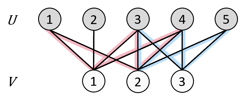
Figure 1. An illustrative example of two $(3,2)$-bicliques.

Lastly, we define the problem that we mainly study:

For example, in Figure 1, there are two $(3,2)$-bicliques: (1) $U^{\prime}=\{1,3,4\},V^{\prime}=\{1,2\}$; (2) $U^{\prime}=\{3,4,5\},V^{\prime}=\{2,3\}$. Their edges are highlighted with pink lines and blue lines, respectively. Therefore, the number of $(3,2)$-bicliques is $2$. It is also known that 1 is NP-Hard (Yang et al., 2021), which means there is no algorithm that runs in polynomial time. Throughout this paper, we assume $p,q\geq 2$.

4. ALGORITHM

In this section, we propose a new sampling-based algorithm called Colored Broom-based Sampling (CBS) that solves 1 approximately.

Inspired by methods for solving $k$-clique counting problems on general graphs (Li et al., 2020; Ye et al., 2022), we start by assigning a color to every vertex on the graph (Section 4.1). Our coloring method is simple, and produces assignments with a small number of colors empirically.

Instead of counting bicliques directly, our next step is to calculate the number of a special motif called ”broom” that we design (Section 4.2). Specifically, the $(p,q)$-broom is defined as follows:

Definition 4.1 (Broom).

Given a bipartite graph $G((U,V),E)$, two vertex sets $U^{\prime}\in U$ and $V^{\prime}\in V$ of size $p$ and $q$, respectively. A vertex ordering is also given: $\{u_{1},u_{2},\dots,u_{p}\}$ and $\{v_{1},v_{2},\dots,v_{q}\}$. The corresponding $(p,q)$-broom is the subgraph $G^{\prime}((U^{\prime},V^{\prime}),E^{\prime})\in G$ that satisfies $E^{\prime}=\{(u_{i},v_{\lfloor\frac{(i-1)(q-1)}{p-1}+1\rfloor})\mid 1\leq i\leq p\}\cup\{(u_{\lceil\frac{(i-1)(p-1)}{q-1}\rceil},v_{i})\mid 2\leq i\leq q\}.$

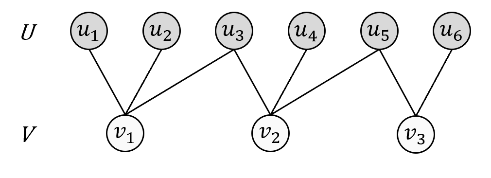
Figure 2. An illustrative example of a $(6,3)$-broom.

In Figure 2, we provide an illustration of a $(6,3)$-broom. We can observe that such a subgraph is, in fact, a tree, which contains $p+q-1$ edges and is connected. As shown in Figure 2, we can clearly see that each vertex $v_{i}$ in $V$ connects to the $2-3$ vertices $u_{j}$ in $U$ that $i$ and $j$ are close. Note that the defined ordering is only used to characterize the pattern, providing a better visualization, and it does not have to align with the original vertex index. Visually speaking, a $(p,q)$-broom is the ”skeleton” of a $(p,q)$-biclique. The general idea here is to design a way to sparsify the dense biclique while trying best to preserve its identity. This broom pattern is very different from EP/Zz++ (Ye et al., 2023)’s $h$-zigzag patterns, as they only use a simple path. We then empirically show that such pattern’s count can lead to a much better approximation of biclique counting.

There are at least two observations for the broom:

1. A spanning tree captures a subgraph better than a simple path.

2. All $p+q-1$ edges are allocated to each vertex nearly evenly.

This distribution design limits the total number of existing brooms, which makes the error analysis tight. Despite its complicated structures, we show in Section 4.2 that its amount can be computed precisely and efficiently using a dynamic programming process with respect to color assignment.

Lastly, by sampling, we extract the quantity relationship between the $(p,q)$-brooms and $(p,q)$-bicliques in the graph and eventually compute our approximate answer (Section 4.3). Shown in Section 5, our algorithm produces high-accuracy approximate counting with faster runtime in real-world datasets. We also prove unbiasedness and provide an error guarantee for our algorithm.

4.1. Coloring

The color assignment should guarantee that for any $(p,q)$-clique $H$, there are no two vertices in $U(H)$ that share the same color. Similarly, the same is true for any two vertices in $V(H)$.

Our coloring algorithm is shown in Algorithm 1. We run the coloring process CalcColor for the vertices in $U$ and $V$ separately (Algorithm 1, 1). Note that here, we consider the neighbor symmetrically. After preprocessing the input graph $G$ with Algorithm 1, each vertex $x\in U\bigcup V$ is colored, and we denote its color as $c(x)$.

$S$ denotes the set of vertices that has not been colored. Whenever $S$ is not empty (Algorithm 1), we will try coloring some vertices with a new color, denoted as $\kappa$. For brevity, we initialize $\kappa$ to be $1$ (Algorithm 1), and whenever we need a new color, we increase $\kappa$ by $1$ (Algorithm 1). $Cnt$ is a temporary array that is used to guarantee the coloring is legal. Specifically, when we try coloring with color $\kappa$, $Cnt[u]$ stores the number of $v$ that satisfies $v\in N(u,G)$ and there exists $w\in N(v,G)$ such that $c(w)=\kappa$. In each round of coloring, we start by initializing $Cnt$ to be all zeros (Algorithm 1). We use $S_{next}$ to store vertices that have to be colored in the next round, initialized as $\emptyset$ (Algorithm 1). We enumerate vertices in $S$ in a randomized order (Algorithm 1). For each enumerated vertex $u$, we first set its color to be $\kappa$ (Algorithm 1) and update $Cnt$ correspondingly (Algorithm 1). If there exists a vertex $x$ such that $Cnt[x]\geq q$ (Algorithm 1), then there could exist a $(p,q)$-biclique with two vertices with the same color. Therefore, such coloring is illegal, and we cannot color $u$ with $\kappa$. In such case, we first revert the changes in $Cnt$ (Algorithm 1) and add $u$ into $S_{next}$ (Algorithm 1). In the end, we have tried every vertex in $S$ at least once and have deferred some vertices’ coloring to upcoming rounds. We assign $S_{next}$ to $S$ and continue (Algorithm 1).

It is not hard to see that the runtime of this coloring process is dominated by the total time of the total number of colors, i,e. $\kappa$. Note that querying, updating, and reverting $cnt$ can be done in $O(|N(u,G)|)$ each operation. In all, the time complexity is $O(\kappa|E|)$. Shown in Table 1, on real-world datasets, $\kappa$ is not large and our coloring algorithm runs very efficiently in turn. The only question left is how such an algorithm guarantees a correct color assignment. We prove it in the following lemma.

Lemma 4.2.

After executing Coloring$(G,p,q)$, for any $(p,q)$-clique $H$ in $G$, there are no two vertices $x,y$ either both in $U(H)$ or in $V(H)$ that share the same color, i.e. $c(x)=c(y)$.

Proof.

Let $U(H)=\{u_{1},u_{2},\dots,u_{p}\}$, $V(H)=\{v_{1},v_{2},\dots,v_{q}\}$. Because of symmetry, we only prove the case of $U$ and $p$. We assume that there are two vertices $u_{1},u_{2}\in U(H)$ with the same color, i.e. $c(u_{1})=c(u_{2})=k$. WLOG, when we color vertices with the $k$-th color, we first set $c(u_{1})\leftarrow k$. Then we will have $Cnt[u_{2}]\geq q$ since $\{v_{1},v_{2},\dots,v_{q}\}$ are $u_{2}$’s neighbors and they all have neighbor $u_{1}$ such that $c(u_{1})=k$. So $u_{2}$ cannot be colored in this round. This contradicts the assumption.

∎

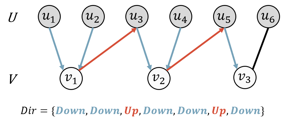
Figure 3. An example of edges’ directions in a $(6,3)$-broom, where edges with different directions are represented by Up and Down in $Dir$ and colored in red and blue, respectively.

Input: $G$: a bipartite graph; $p,q$: two parameters.

Output: $G^{\prime}$: a colored bipartite graph.

1

2CalcColor$(G,U(G),p,q)$;

3 CalcColor$(G,V(G),q,p)$;

4 $G^{\prime}\leftarrow G$;

5

6return $G^{\prime}$;

7Procedure CalcColor$(G,S,p,q)$

8    Initialize $\kappa\leftarrow 1$;

9    while $|S|>0$ do

10       Initialize an array $Cnt$ with zeros;

11       $S_{next}\leftarrow\emptyset$;

       /* enumerate vertices in a random order */

12       for $u\in S$ do

13          $c(u)\leftarrow\kappa$;

14          Update $Cnt$;

15          if $\exists x,Cnt[x]\geq q$ then

16             Revert $Cnt$’s change;

17             $S_{next}\leftarrow S_{next}\cup\{u\}$;

18            

19         

20      $\kappa\leftarrow\kappa+1$;

21       $S\leftarrow S_{next}$;

22      

23   

Algorithm 1 CBS: Coloring

4.2. Pattern Counting

After coloring, we enhance the motif we are counting with a condition of distinct color. However, it is still hard to count bicliques directly. Instead, we count the number of $(p,q)$-brooms. Since we assign a concrete integer for each color in Algorithm 1 for any $(p,q)$-biclique, to avoid overcounting, we assume its vertex ordering of $U^{\prime}$ and $V^{\prime}$ is following the color from small to large. With this exact ordering, by Definition 4.1, there is exactly one $(p,q)$-broom subgraph in each $(p,q)$-biclique. Note that the color of these $(p,q)$-brooms is also unique, which is convenient for counting. Algorithm 2 is able to compute the number of $(p,q)$-brooms of this type. We then show how to use this value to approximate the biclique count.

The whole process is dynamic programming where its state is represented by the total number of edges we have accumulated so far and the last edge we keep track of. To well define this dynamic programming state, we need to specify a few more properties in this type of $(p,q)$-broom:

A. Any $(p,q)$-broom $H$ is connected and contains exactly $p+q-1$ edges. That is to say, it is actually a tree.

B. If we sort all edges $(u,v)\in E(H)$ by the increasing order of the tuple $(c(u),c(v))$, there is only three types of edges:

1. The edge with the maximum tuple.

2. Edges sharing an endpoint in $U(H)$ with the next edge.

3. Edges sharing an endpoint in $V(H)$ with the next edge.

For (2) and (3), we signal them with a ”direction” as either Up or Down. For example, as shown in the $(6,3)$-broom in Figure 3, $(u_{1},v_{1})$ is with the smallest partial order. Its direction is Down since it shares the same endpoint $v_{1}$ with the next edge $(u_{2},v_{1})$. Similarly, $(u_{2},v_{1})$, $(u_{3},v_{2})$, $(u_{4},v_{2})$, $(u_{5},v_{3})$ are also with direction Down, highlighted with blue arrows. $(u_{3},v_{1})$, $(u_{5},v_{2})$ are with direction Up, highlighted with reversed red arrows. $(u_{6},v_{3})$ has no direction since it is the edge with the maximum tuple.

After fixing the structure and order of edges by B, we can simply use the number of edges and the last edge to represent the current structure of the growing broom. The rest is enumeration and direct transition. The details are as follows.

To begin with, we sort $U(G)$, $V(G)$ by the increasing order of colors $c(u),c(v)$ (Algorithm 2), and sort $E(G)$ by the increasing order of the color tuple $(c(u),c(v))$ (Algorithm 2). We use a 2D table $Dp[len][pre]$ to store the count of each state, indicating the current number of edges $len$ and the last edge $pre$. We first initialize the whole table to $0$ (Algorithm 2). Then for the case where each $(u,v)$ acts as the first edge in the broom, we set $Dp[1][(u,v)]$ to be $1$ (Algorithm 2, 2). Since there are $p+q-1$ edges in total besides the first one, the first dimension of the table should be $1$ to $p+q-1$. We iterate this dimension from small to large to accumulate the growing broom from $1..t$-th edges to $1..t+1$-th edges (Algorithm 2). We use $Dir[t]$ to denote the $t$-th edge’s direction in the $(p,q)$-broom. When $Dir[t]$ is Up (Algorithm 2), the $t+1$-th edge and the $t$-th edge share a common point in $U$. Therefore, for each edge $(u,v)$ (Algorithm 2), $Dp[t+1][(u,v)]$ should accumulate the number of ways coming from any $Dp[t][(u,w)]$ such that $w$ is in $N(u,G)$ and $c(w)<c(v)$ (Algorithm 2). Similarly, when $Dir[t]$ is Down (Algorithm 2), the $t+1$-th edge and the $t$-th edge share a common point in $V$. In this case, $Dp[t+1][(u,v)]$ should accumulate the number of ways coming from any $Dp[t][(w,v)]$ such that $w$ is in $N(v,G)$ and $c(w)<c(u)$ (Algorithm 2, 2). After all computations, we return $B$ as the sum of all $Dp[p+q-1][\cdot]$ and the $Dp$ table as the results (Algorithm 2).

By using the prefix sum technique, for each iteration, we can finish all transition computations in $O(|E|)$. There are $O(p+q)$ rounds. Therefore, the total time complexity is $O((p+q)|E|)$.

Input: $G$: a colored bipartite graph; $p,q$: two parameters.

Output: $Dp$: a $2D$ array; $B$: the total number of $(p,q)$-brooms in $G$.

1

2Sort $U(G),V(G)$ by the increasing order of $c(u),c(v)$;

3 Sort $E(G)$ by the increasing order of $(c(u),c(v))$;

4

5Initialize $Dp$ with zeros;

6

7for $(u,v)\in E(G)$ do  $Dp[1][(u,v)]\leftarrow 1$ ;

8 for $t\leftarrow 1$ to $p+q-2$ do

9    if $Dir[t]=\texttt{Up}$ then

10       for $(u,v)\in E(G)$ do

11          $Dp[t+1][(u,v)]\leftarrow\sum_{w\in N(u,G),c(w)<c(v)}Dp[t][(u,w)]$;

12         

13      

14    else

15       for $(u,v)\in E(G)$ do

16          $Dp[t+1][(u,v)]\leftarrow\sum_{w\in N(v,G),c(w)<c(u)}Dp[t][(w,v)]$;

17         

18      

19   

20$B\leftarrow\sum_{(u,v)\in E(G)}Dp[p+q-1][(u,v)]$;

21

return $Dp,B$;

Algorithm 2 CBS: CountingIndex

4.3. Approximate Counting via Sampling

After CountingIndex$(G,p,q)$, we have accumulated $B$ $(p,q)$-brooms. To approximate the quantity relation between our computed $(p,q)$-brooms and $(p,q)$-bicliques, we can do the following sampling process:

1. Set two counters $cnt_{broom}$ and $cnt_{biclique}$.

2. Uniformly sample a $(p,q)$-broom $P$ from all $B$ ones and increase $cnt_{broom}$ by $1$.

3. If the induced subgraph by $U(P)$ and $V(P)$ is a $(p,q)$-biclique, increase $cnt_{biclique}$ by $1$.

After applying this sampling process sufficiently many times, we can roughly approximate the number of $(p,q)$-bicliques by $cnt_{biclique}/cnt_{broom}\times B$.

However, such a sampling process is too inefficient. We now propose Algorithm 3 to accelerate this process, utilizing the computed dynamic programming results from CountingIndex$(G,p,q)$. Recall that $Dp[t][(u,v)]$ represents the number of ways to build a growing $(p,q)$-broom til the $t$-th edge, which is $(u,v)$.

To begin with, we start by sampling the last edge of the $(p,q)$-broom, denoted as $(u_{last},v_{last})$ (Algorithm 3). Here, the sampling should follow the weight distribution of $\{Dp[p+q-1][\cdot]\}$, indicating how many $(p,q)$-brooms end with each edge. The following process is similar to reverting the dynamic programming process. Instead of building the $(p,q)$-broom from the $1$-st edge to the $(p+q-1)$-th edge, we do it reversely. We use $(u_{cur},v_{cur})$, $U^{\prime}$, $V^{\prime}$ to denote the current growing $(p,q)$-broom. They are initialized as $(u_{last},v_{last})$, $\{u_{last}\}$, $\{v_{last}\}$ respectively (Algorithm 3, 3). Specifically, since $(u_{last},v_{last})$ is the $(p+q-1)$-th edge, we are now adding the $(p+q-2)$-th edge til the $1$-th edge gradually (Algorithm 3). Assume we are processing the $i$-th edge now, and we know the $(i+1)$-th edge is $(u_{cur},v_{cur})$. We initialize an edge set $S$ to store the candidate edge for the $i$-th edge. Based on the direction signaling, we can know whether it should share the common endpoint in $U$ or $V$. If $Dir[i]$ is Up (Algorithm 3), then we should find all $w\in N(u_{cur},G)$ such that $c(w)<c(v_{cur})$ and $U^{\prime}\subseteq N(w,G)$. We assign $S$ to be $\{(u_{cur},w)\}$ (Algorithm 3). The first condition is for obeying the color order, and the second condition indicates that adding $w$ can still guarantee that the induced subgraph is biclique. Similarly, if $Dir[i]$ is Down (Algorithm 3), we find all all $w\in N(v_{cur},G)$ such that $c(w)<c(u_{cur})$ and $V^{\prime}\subseteq N(w,G)$. Then we assign $S$ to be $\{(w,v_{cur})\}$ (Algorithm 3).

The idea to accelerate the sampling is, by building the $(p,q)$-broom, we strictly guarantee that it will correspond to a $(p,q)$-biclique while keeping track of the probability of sampling out this $(p,q)$-broom, which can be computed through the dynamic programming table. In the beginning, we initialize $ans$ to be $1$ (Algorithm 3). Then, for the $i$-th edge, the probability contribution of sampling it out from $S$ should be the number of the growing broom ends with $(u,v)\in S$ divided by the total number of possible brooms at this step, which is $\frac{\sum_{(u,v)\in S}Dp[i][(u,v)]}{Dp[i+1][(u_{cur},v_{cur})]}$. We multiply $ans$ by this value (Algorithm 3). If $ans$ becomes $0$, then there is no possible $(p,q)$-biclique from the current sampled $(p,q)$-broom. We return with $0$ in this case (Algorithm 3). Now we are ready to sample the $i$-th edge from $S$ (Algorithm 3). We do so following the normalized distribution of possible brooms from this step ($\{Dp[i][\cdot]\}$). To continue the process, we assign $(u_{cur},v_{cur})$, $U^{\prime}$, $V^{\prime}$ to $(u_{next},v_{next})$, $U^{\prime}\cup\{u_{next}\}$, $V^{\prime}\cup\{v_{next}\}$, respectively (Algorithm 3, 3).

In the end, we successfully sample a $(p,q)$-broom that corresponds to one $(p,q)$-biclique and compute the probability of sampling it out. We return this probability by multiplying $B$ as the approximate count of $(p,q)$-bicliques (Algorithm 3).

It is not hard to see that the time complexity is dominated by the cost of updating $S$, which requires enumerating all neighbors. The loop only lasts $O(p+q)$. Therefore, the time complexity is $O((p+q)\times\Delta)$, where $\Delta$ denotes the maximal degree in $G$.

Input: $G$: a colored bipartite graph; $p,q$: two parameters; $Dp$: a $2D$ array; $B$: the total number of $(p,q)$-brooms in $G$.

Output: $ans$: estimate number of $(p,q)$-clique in $G$.

1 Sample the last edge $(u_{last},v_{last})$ in $E(G)$ following the weight distribution of brooms;

2 $(u_{cur},v_{cur})\leftarrow(u_{last},v_{last})$;

3

4$U^{\prime}\leftarrow\{u_{last}\},\ V^{\prime}\leftarrow\{v_{last}\}$;

5

6$ans\leftarrow 1$;

7 for $i\leftarrow p+q-2$ to $1$ do

8    Initialize set $S\leftarrow\emptyset$;

9    if $Dir[i]=\texttt{Up}$ then

10       $S\leftarrow\{(u_{cur},w)\ |\ w\in N(u_{cur},G),c(w)<c(v_{cur}),U^{\prime}\subseteq N(w,G)\}$;

11      

12    else

13       $S\leftarrow\{(w,v_{cur})\ |\ w\in N(v_{cur},G),c(w)<c(u_{cur}),V^{\prime}\subseteq N(w,G)\}$;

14      

15   $ans\leftarrow ans\times\frac{\sum_{(u,v)\in S}Dp[i][(u,v)]}{Dp[i+1][(u_{cur},v_{cur})]}$;

16    if $ans=0$ then  break ;

17    Sample the next edge $(u_{next},v_{next})$ in $S$ following the weight distribution of growing brooms;

18    $(u_{cur},v_{cur})\leftarrow(u_{next},v_{next})$;

19    $U^{\prime}\leftarrow U^{\prime}\cup\{u_{next}\},V^{\prime}\leftarrow V^{\prime}\cup\{v_{next}\}$;

20   

return $ans\times B$;

Algorithm 3 CBS: Sampling

Overall Algorithm. We provide Algorithm 4 as a black box to call all three subroutines properly and output the estimated answer of the biclique count. We start by coloring (Algorithm 4) and pattern counting (Algorithm 4). Then by the input sampling size parameter $T$, we repeatedly call Sampling$(G,p,q,Dp,B)$ and aggregate the return to $\hat{C}$. The output approximate $(p,q)$-biclique count is the average of all $T$ attempts (Algorithm 4). Note that as a common trick, we will execute core-reduction for the original graph (Yang et al., 2021): For any query $(p,q)$, we split the graph and reduce the query pair to $(p-1,q)$.

Input: $G$: a bipartite graph; $p,q$: two parameters; $T$: sampling times.

Output: $\hat{C}$: estimate number of $(p,q)$-clique.

1 $G\leftarrow\$ Coloring$(G,p,q)$;

2 $Dp,B\leftarrow\$ CountingIndex$(G,p,q)$;

3 $\hat{C}\leftarrow 0$;

4 for $i\leftarrow 1$ to $T$ do

5    $\hat{C}\leftarrow\hat{C}\ +$ Sampling$(G,p,q,Dp,B)$;

6$\hat{C}\leftarrow\hat{C}/T$;

7

return $\hat{C}$;

Algorithm 4 CBS: Main

Unbiasedness. We now show that the CBS method is unbiased. Let $(u_{cur},v_{cur})$, $U^{\prime}$, and $V^{\prime}$ represent the current growing $(p,q)$-broom. For clarity, we introduce the following definitions:

• $\mathcal{F}_{U^{\prime},V^{\prime}}$: The total value to be multiplied into $ans$, defined as the product of the last $i=(p+q)-(|U^{\prime}|+|V^{\prime}|)$ fractions.

• $\mathcal{B}_{U^{\prime},V^{\prime}}$: The number of $(p,q)$-brooms $H$ such that $U^{\prime},V^{\prime}$ are the maximal tuples of $U(H)$ and $V(H)$.

• $\mathcal{C}_{U^{\prime},V^{\prime}}$: The number of $(p,q)$-bicliques $H^{\prime}$ such that $U^{\prime},V^{\prime}$ are the maximal tuples of $U(H^{\prime})$ and $V(H^{\prime})$.

After that, we prove the following lemma by mathematical induction.

Lemma 4.3.

For any growing $(p,q)$-broom $U^{\prime},V^{\prime}$, $\mathbb{E}\left[\mathcal{F}_{U^{\prime},V^{\prime}}\right]=\mathcal{C}_{U^{\prime},V^{\prime}}/\mathcal{B}_{U^{\prime},V^{\prime}}.$

Proof.

(a) When $|U^{\prime}|+|V^{\prime}|=p+q$, we have $\mathcal{B}_{U^{\prime},V^{\prime}}=1$. In this case, $\mathcal{F}_{U^{\prime},V^{\prime}}=\mathcal{C}_{U^{\prime},V^{\prime}}=1$ if $U^{\prime},V^{\prime}$ forms a $(p,q)$-biclique; otherwise $\mathcal{F}_{U^{\prime},V^{\prime}}=\mathcal{C}_{U^{\prime},V^{\prime}}=0$. Hence, $\mathbb{E}\left[\mathcal{F}_{U^{\prime},V^{\prime}}\right]=\mathcal{C}_{U^{\prime},V^{\prime}}/\mathcal{B}_{U^{\prime},V^{\prime}}$ trivially holds in this case. (b) Suppose that the lemma holds for all growing $(p,q)$-brooms with $\ |U^{\prime}|+|V^{\prime}|=k+1$ . For any broom with $|U^{\prime}|+|V^{\prime}|=k$, let $P=\frac{\sum_{(u,v)\in S}Dp[i][(u,v)]}{Dp[i+1][(u_{cur},v_{cur})]}$. We then have

$$\mathbb{E}\left[\mathcal{F}_{U^{\prime},V^{\prime}}\right]=P\sum\limits_{(u,v)\in S}\frac{Dp[i][(u,v)]}{\sum\limits_{(u,v)\in S}Dp[i][(u,v)]}\mathbb{E}\left[\mathcal{F}_{U^{\prime}\cup\{u\},V^{\prime}\cup\{v\}}\right].$$

Since $u_{cur}=u$ or $v_{cur}=v$ always holds, we have that $|U^{\prime}\cup\{u\}|+|V^{\prime}\cup\{v\}|=|U|+|V|+1=k+1$. According to the definition of $Dp$ and $\mathcal{B}$, We can derive that $Dp[i][(u,v)]=\mathcal{B}_{U^{\prime}\cup\{u\},V^{\prime}\cup\{v\}}$, and thus

$$\mathbb{E}\left[\mathcal{F}_{U^{\prime},V^{\prime}}\right] =\frac{\sum\limits_{(u,v)\in S}Dp[i][(u,v)]\frac{\mathcal{C}_{U^{\prime}\cup\{u\},V^{\prime}\cup\{v\}}}{\mathcal{B}_{U^{\prime}\cup\{u\},V^{\prime}\cup\{v\}}}}{Dp[i+1][(u_{cur},v_{cur})]}$$

$$=\frac{\sum\limits_{(u,v)\in S}\mathcal{C}_{U^{\prime}\cup\{u\},V^{\prime}\cup\{v\}}}{\mathcal{B}_{U^{\prime},V^{\prime}}}$$

$$=\frac{\mathcal{C}_{U^{\prime},V^{\prime}}}{\mathcal{B}_{U^{\prime},V^{\prime}}},$$

where the last equation is because $\mathcal{C}_{U^{\prime}\cup\{u\},V^{\prime}\cup\{v\}}=0$ for all pairs of $(u,v)\notin S$. ∎

Then we can derive the following theorem:

Theorem 4.4.

Let $ans_{i}$ be the value of $ans$ in the $i$-th sampling. Let $\hat{C}=\frac{1}{T}\sum_{i=1}^{T}ans_{i}\times B$. Then $\hat{C}$ is an unbiased estimator of the number of $(p,q)$-bicliques in $G$.

Proof.

We first have the following induction by Lemma 4.3:

$$\mathbb{E}\left[ans_{i}\times B\right]$$

$$=B\times\sum\limits_{(u,v)\in E(G)}\frac{Dp[p+q-1][(u,v)]}{\sum Dp[p+q-1][(u,v)]}\mathbb{E}\left[\mathcal{F}_{\{u\},\{v\}}\right]$$

$$=\sum\limits_{(u,v)\in E(G)}Dp[p+q-1][(u,v)]\times\mathbb{E}\left[\mathcal{F}_{\{u\},\{v\}}\right]$$

$$=\sum\limits_{(u,v)\in E(G)}\mathcal{C}_{\{u\},\{v\}}=\mathcal{C}_{\emptyset,\emptyset}.$$

Then we can derive that: $\mathbb{E}\left[\hat{C}\right]=\frac{1}{T}\sum_{i=1}^{T}\mathbb{E}\left[ans_{i}\times B\right]=\mathcal{C}_{\emptyset,\emptyset}$. Note that $\mathcal{C}_{\emptyset,\emptyset}$ is the number of $(p,q)$-bicliques in $G$ according to the definition. Therefore, $\hat{C}$ is an unbiased estimator of the number of $(p,q)$-bicliques in $G$. ∎

Based on Theorem 4.4, we have obtained an unbiased estimator $\hat{C}$ of the number of $(p,q)$-bicliques in Algorithm 4.

Error Analysis. we now analyze the estimation error of our sampling algorithms. Our analysis relies on the classic Hoeffding’s inequalities, which are shown below.

Lemma 4.5 (Hoeffding’s inequality, (Chernoff, 1952; Hoeffding, 1994)).

For the random variables $X_{i}\in[0,M]$,$1\leq i\leq n$, we let $X=\sum_{i=1}^{n}X_{i}$. Then for $\epsilon>0$, we have

$$\Pr(X\geq(1+\epsilon)\mathbb{E}\left[X\right]) \leq\exp(-\frac{2\epsilon^{2}\mathbb{E}\left[X\right]^{2}}{nZ^{2}}),$$

$$\Pr(X\leq(1-\epsilon)\mathbb{E}\left[X\right]) \leq\exp(-\frac{2\epsilon^{2}\mathbb{E}\left[X\right]^{2}}{nZ^{2}}).$$

Based on Lemma 4.5, we can derive the estimation error of our algorithms as shown in the following theorem.

Theorem 4.6.

Let $C,B$ be the number of $(p,q)$-bicliques, $(p,q)$-brooms, respectively. Let $\hat{C}=\frac{1}{T}\sum_{i=1}^{T}ans_{i}\times B$ denote the estimated number of $(p,q)$-bicliques, where $ans_{i}$ is the return result in the $i$-th sampling. Then, $\hat{C}$ is a $(1+\epsilon)$ approximation of $C$ with probability $(1-\alpha)$ if $T\geq\frac{B^{2}}{2\epsilon^{2}C^{2}}\ln(\frac{2}{\alpha})$.

Proof.

We can derive $ans_{i}\times B\in[0,B]$ since the values multiplied to $ans$ are all probabilities in $[0,1]$. And we have $\mathbb{E}\left[\hat{C}T\right]=CT$ based on Theorem 4.4. Given a positive value $\epsilon$, applying Lemma 4.5 by plugging in $n=T$, $X_{i}=ans_{i}\times B$, $X=\sum_{i=1}^{n}X_{i}=\hat{C}T$, we then have

$$\Pr(X\geq(1+\epsilon)\mathbb{E}\left[X\right]) =\Pr(\hat{C}T\geq(1+\epsilon)CT)\leq\exp(-\frac{2\epsilon^{2}(CT)^{2}}{TB^{2}}),$$

$$\Pr(X\leq(1-\epsilon)\mathbb{E}\left[X\right]) =\Pr(\hat{C}T\leq(1-\epsilon)CT)\leq\exp(-\frac{2\epsilon^{2}(CT)^{2}}{TB^{2}}).$$

Further, we have

$$\Pr(\frac{|\hat{C}-C|}{C}\geq\epsilon)\leq 2\exp(-\frac{2\epsilon^{2}C^{2}T}{B^{2}})$$

Let $2\exp(-\frac{2\epsilon^{2}C^{2}T}{B^{2}})\leq\alpha$, we can derive that $T\geq\frac{B^{2}}{2\epsilon^{2}C^{2}}\ln(\frac{2}{\alpha})$. ∎

From Theorem 4.6, the sample size $T$ is mainly determined by $(\frac{B}{C})^{2}$. That is to say, we need a larger sample size $T$ to ensure high accuracy with a larger $(\frac{B}{C})^{2}$, where $B$ is the number of $(p,q)$-brooms, $C$ is the number of $(p,q)$-bicliques. As shown in Section A.3, $(\frac{B}{C})^{2}$ is usually small. Therefore, our algorithm generally does not need a large $T$ to achieve good accuracy in real-world datasets.

5. EVALUATION

Table 1. Datasets used in experiments.

Graphs (Abbr.)	Category	$|U|$	$|V|$	$|E|$	$\max\kappa$
github (GH)	Authorship	56,519	120,867	440,237	508
StackOF (SO)	Rating	545,195	96,678	1,301,942	290
Twitter (Wut)	Interaction	175,214	530,418	1,890,661	2933
IMDB (IMDB)	Affiliation	685,568	186,414	2,715,604	158
Actor2 (Actor2)	Affiliation	303,617	896,302	3,782,463	189
Amazon (AR)	Rating	2,146,057	1,230,915	5,743,258	155
DBLP (DBLP)	Authorship	1,953,085	5,624,219	12,282,059	126
Epinions (ER)	Rating	120,492	755,760	13,668,320	13200
Wikipedia-edits-de (DE)	Authorship	1,025,084	5,910,432	129,885,939	118356

5.1. Experimental Setting

Datasets. We use nine real datasets from different domains, which are available at SNAP (Project, 2009), Laboratory of Web Algorithmics (of Web Algorithmics, 2013), and Konect  (Konect, 2006). Table 1 shows the statistics of these graphs.

Baselines. We compare our method with the baselines from highly related works. We summarize the core ideas of each baseline method as follows.

• BCList++ (Yang et al., 2021): the biclique listing-based algorithm, which is based on the Bron-Kerbosch algorithm (Bron and Kerbosch, 1973). The key idea of BCList++ is to iteratively enumerate all $(p,q)$-bicliques containing each vertex through a node expansion process. Specifically, it employs an ordering-based search paradigm, where for each vertex, only its higher-order neighbors are considered during enumeration. Additionally, a graph reduction technique is applied to reduce the search space before biclique counting.

• EPivoter (Ye et al., 2023): the state-of-the-art algorithm for exact biclique counting, which relies on the edge-based pivot technique. In EPivoter, an edge-based search framework is introduced. Unlike BCList++, it iteratively selects edges from the candidate set (i.e., the edge set used for biclique expansion) to expand the current biclique. Specifically, during the enumeration process, in each branch, it first select one edge as the pivot edge, and based on this edge, vertices can be grouped into four disjoint groups. By storing the entire enumeration tree along with the four vertex sets, biclique counting can then be efficiently performed using combination counting.

• EP/Zz++ (Ye et al., 2023): the state-of-the-art algorithm for approximate biclique counting. It first partitions the graph into two regions: a dense region (a subgraph containing only high-degree vertices) and a sparse region (a subgraph containing only low-degree vertices). For the sparse region, EP/Zz++ utilizes EPivoter for exact counting, while for the dense region, it proposes a zigzag path-based sampling algorithm for approximate counting. Specifically, it leverages the fact that a $(p,q)$-biclique must contain a fixed number of $(min\{p,q\})$-zigzag paths. Based on this property, the algorithm first counts the number of $h$-zigzag paths and then samples $T$ such paths, where $h=min\{p,q\}$. Finally, it estimates the number of $h$-bicliques based on their proportion with the sampled paths.

• CBS: our proposed approximation algorithm, which is introduced in Section 4.

Notice that we compare EP/Zz++ instead of EP/Zz (Ye et al., 2023), since the former one is a better version of the latter in terms of efficiency and accuracy. We implement all the algorithms in C++ and run experiments on a machine having an Intel(R) Xeon(R) Platinum 8358 CPU @ 2.60GHz and 512GB of memory, with Ubuntu installed.

Parameter Settings. In our experiments, we following the existing work (Ye et al., 2023) setting $T$=$10^{5}$ as default values. We define the estimation error as $\frac{|\hat{C}-C|}{C}$, where $C$ denotes the exact count of bicliques, and $\hat{C}$ represents its approximated value. To ensure the reliability of our results, we run each approximation algorithm 10 times, with the reported error representing the average across these executions. For some datasets, the exact count of bicliques cannot be computed (e.g., ER and DE), we evaluate the estimation error differently by using the average approximated biclique count from 10 runs as the exact count (i.e., $C$).

5.2. Overall Comparison Results

In this section, we compare CBS with three competitors (introduced in Section 5.1), w.r.t. overall efficiency, accuracy, and the effect of $p$ and $q$, and the number of samples to demonstrate the superior of our algorithm.

1. Efficiency of All Algorithms. Figure 4 depicts the average running time of all the biclique counting algorithms on nine datasets for counting all $3\leq p,q\leq 9$ bicliques. We make the following observations and analysis: (1) Our method CBS is up to two orders of magnitude faster than all competitors, this is mainly because our algorithm has a better theoretical guarantee. (2) on almost all datasets, CBS is at least $10\times$ faster than all methods, except DBLP dataset. On this dataset, BCList++ achieves the best performance, as graph reduction significantly reduces $|U|$ and $|V|$, allowing it to perform efficiently without extra initialization steps. Meanwhile, CBS still outperforms EPivoter and EP/Zz++. (3) On the two largest datasets, ER and DE, the exact algorithms fail to count the bicliques within $10^{5}$ seconds, while both approximate algorithms successfully complete the task. Our method, CBS, demonstrates at least 3 times faster performance compared to EP/Zz++.

Figure 4. Average runtime of different biclique counting algorithms for all $3\leq p,q\leq 9$.

Figure 5. Average error of EP/Zz++ and CBS for all $3\leq p,q\leq 9$.

2. Accuracy of All Algorithms. Figure 5 illustrates the average error rates of CBS and EP/Zz++ across all datasets for biclique sizes ranging from 3 to 9 (i.e., $3\leq p,q\leq 9$). We can see that our algorithm demonstrates up to a $8\times$ reduction in error compared to EP/Zz++, thanks to our carefully designed coloring scheme and $(p,q)$-broom-based sampling technique. Note that for the first three smaller datasets, EP/Zz++ exhibits significant errors, with at least 38.9% inaccuracy, rendering its results unreliable. In contrast, our method, CBS, maintains a maximum error rate of 16.9% under the same number of sampling rounds. Combining these observations with the performance results shown in Figure 4, we can conclude that our algorithm demonstrates an even greater advantage when considering the trade-off between accuracy and efficiency. This indicates that to achieve the same error rate, our algorithm would likely exhibit an even more substantial performance advantage over EP/Zz++.

3. Effect of $p$ and $q$. Figures LABEL:figure:sampling_time_heatmap and LABEL:figure:error_heatmap illustrate the sampling time and error rate, respectively, of CBS and EP/Zz++ across various $p$ and $q$ values. In each figure, rows represent $p$ values and columns represent $q$ values. Each cell displays the sampling time (in Figure LABEL:figure:sampling_time_heatmap) or the estimation error (in Figure LABEL:figure:error_heatmap) for counting the corresponding $(p,q)$-bicliques. Clear, our method, CBS, outperforms EP/Zz++ by up to two orders of magnitude in both sampling time and accuracy. For instance, with $p=5$ and $q=3$ on the ER dataset, EP/Zz++ requires 822.6 seconds for sampling, whereas our algorithm completes this stage in just 5.3 seconds. In terms of accuracy, on the Wut dataset with $p=5$ and $q=7$, EP/Zz++ has an estimation error of 202.49, while our algorithm achieves a significantly lower error of 1.91. This observation aligns with our analysis in Section 4.

LABEL:Tcurve

LABEL:Errorcurve

4. Effect of $T$. We evaluate the effect of sample numbers on sampling time and error rate. The results on three datasets are shown in Figures LABEL:figure:Timecurve and LABEL:figure:T_curve. Based on these results, we observe the following: (1) For sampling time, our algorithm consistently outperforms EP/Zz++, particularly when the sample numbers are relatively low (e.g., from $10^{1}$ to $10^{3}$). (2) Our algorithm consistently produces more accurate results than EP/Zz++, regardless of whether the sample size is high or low. (3) Even with very few samples, our algorithm achieves acceptable solutions. For instance, on the AR dataset, CBS requires only $10^{3}$ samples to achieve a solution with a $30\%$ error rate, whereas EP/Zz++ requires over $10^{4}$ samples.

Detailed Analysis

In addition, more detailed analysis about CBS is provided in Appendix A, including Ablation Study, Time Cost of Different Stages, and Statistical of the Hyper-parameters. We only summarize the key conclusions here: (1) In high-accuracy scenarios, our coloring technique can significantly improve accuracy without highly impacting sampling time. (2) On more than half of the datasets, our algorithm requires less initializing and sampling time, compared to EP/Zz++. (3) When error rate $\epsilon$ is fixed, our algorithm CBS consistently requires fewer samples than EP/Zz++.

6. CONCLUSION

In this paper, we tackled the $(p,q)$-biclique counting problem in large-scale bipartite graphs, crucial for applications like recommendation systems and cohesive subgraph analysis. To address scalability and accuracy issues in existing methods, we proposed a novel sampling-based algorithm leveraging $(p,q)$-brooms, special spanning trees within $(p,q)$-bicliques. Utilizing graph coloring and dynamic programming, our method efficiently approximates $(p,q)$-biclique counts with unbiased estimates and provable error guarantees. Experimental results on nine real-world datasets show that our approach outperforms state-of-the-art methods, achieving up to 8$\times$ error reduction and 50$\times$ speed-up. Interesting future work includes extending our method to dynamic bipartite graphs with evolving structures and exploring its application to counting motifs/cliques in heterogeneous information networks.

Appendix A Detailed Analysis

In this section, we extensively evaluate and analyze CBS from different angles.

A.1. Ablation Study

To evaluate the effect of our coloring technique, we design a new variant of CBS by removing the vertex coloring step, denoted by BS. We then run them on two datasets and report the results in Figure 9. As we shall see, CBS generally achieves lower error with the same number of samples, aligning with our previous analysis. While the coloring technique slightly increases sampling time initially, the gap diminishes as sampling iterations increase. This demonstrates that in high-accuracy scenarios, our coloring technique can significantly improve accuracy without highly impacting sampling time.

$T$	AR		Wut
	BS	CBS	BS	CBS
$10^{2}$	72.75	81.63	60.60	37.70
$10^{3}$	43.33	28.47	22.03	23.50
$10^{4}$	13.08	11.54	13.51	12.64
$10^{5}$	4.37	3.35	5.11	4.59
$10^{6}$	1.35	1.13	1.71	1.43

Figure 9. Results of BS and CBS with varying $T$.

A.2. Time Cost of Different Stages

For the two approximation algorithms, CBS and EP/Zz++, both require an initialization stage to precompute some auxiliary data for sampling. Specifically, in CBS, we need to assign a color number for each vertex (i.e., coloring) and count the number of $(p,q)$-brooms in bipartite graph, while in EP/Zz++, it needs to count the number of $h$-zigzag paths bipartite graph, where $h$ = $\min\{p,q\}$. In Figure  10, we report the initializing and sampling times for these algorithms across all datasets. We observe that on more than half of the datasets, our algorithm requires less initializing and sampling time, which indicates that the number of $(p,q)$-brooms in the bipartite graph is typically less than $h$-zigzag paths (using in EP/Zz++). In terms of sampling time, our algorithm is up to two orders of magnitude faster than EP/Zz++. While on two datasets, GH and ER, EP/Zz++ is 10 times faster in initializing, CBS achieves 100 times lower sampling time, making the total time (i.e., initializing plus sampling) of our algorithm still highly efficient.

Figure 10. Average initializing and sampling time of EP/Zz++ and CBS for all $3\leq p,q\leq 9$ ($T=10^{5}$).

A.3. Statistical of the Hyper-parameters

Recall that in CBS and EP/Zz++, when $\epsilon$ is fixed, their required sample sizes are proportional to $\frac{B^{2}}{C^{2}}$ and $\frac{Z^{2}}{\rho^{2}}$, respectively. As shown in Table 2, we report the values of $\frac{B^{2}}{C^{2}}$ and $\frac{Z^{2}}{\rho^{2}}$ on the Amazon dataset for varying $p$ and $q$. Similar trends are observed across other datasets. Based on Table 2, our algorithm CBS consistently requires fewer samples than EP/Zz++, explaining why CBS achieves the same or even lower estimation error with a smaller sample size. For instance, CBS requires up to 88$\times$ fewer samples than EP/Zz++ on $p$ = 5 and $q$ = 9, demonstrating its efficiency in reducing sampling overhead while maintaining accuracy.

Table 2. The value of $\frac{B^{2}}{C^{2}}$ and $\frac{Z^{2}}{\rho^{2}}$ with varying $p,q$ (Amazon).

$(p,q)$	$\frac{B^{2}}{C^{2}}$	$\frac{Z^{2}}{\rho^{2}}$
(3,4)	1.40E+03	1.79E+03
(3,5)	3.97E+03	1.69E+04
(3,9)	4.55E+04	2.85E+05
(4,5)	5.41E+04	5.98E+04
(4,8)	9.27E+04	2.48E+05
(5,3)	3.96E+02	6.17E+03
(5,6)	4.04E+05	1.20E+06
(5,9)	3.77E+04	3.34E+06
(6,4)	5.73E+03	5.80E+04
(6,7)	6.42E+06	5.32E+07
(7,4)	8.07E+03	1.54E+05
(7,7)	7.15E+06	2.44E+07
(8,4)	1.36E+04	3.16E+05
(8,8)	4.74E+07	1.04E+09
(9,4)	2.36E+04	5.32E+05
(9,9)	2.92E+08	8.01E+10

References

- (1)
- Beutel et al. (2013) Alex Beutel, Wanhong Xu, Venkatesan Guruswami, Christopher Palow, and Christos Faloutsos. 2013. Copycatch: stopping group attacks by spotting lockstep behavior in social networks. In Proceedings of the 22nd international conference on World Wide Web. 119–130.
- Borgatti and Everett (1997) Stephen P Borgatti and Martin G Everett. 1997. Network analysis of 2-mode data. Social networks 19, 3 (1997), 243–269.
- Bressan et al. (2018) Marco Bressan, Flavio Chierichetti, Ravi Kumar, Stefano Leucci, and Alessandro Panconesi. 2018. Motif counting beyond five nodes. ACM Transactions on Knowledge Discovery from Data (TKDD) 12, 4 (2018), 1–25.
- Bron and Kerbosch (1973) Coenraad Bron and Joep Kerbosch. 1973. Finding all cliques of an undirected graph (algorithm 457). Commun. ACM 16, 9 (1973), 575–576.
- Cai et al. (2024) Xinwei Cai, Xiangyu Ke, Kai Wang, Lu Chen, Tianming Zhang, Qing Liu, and Yunjun Gao. 2024. Efficient Temporal Butterfly Counting and Enumeration on Temporal Bipartite Graphs. Proc. VLDB Endow. 17, 4 (mar 2024), 657–670. https://doi.org/10.14778/3636218.3636223
- Chen et al. (2020) Hongxu Chen, Hongzhi Yin, Tong Chen, Weiqing Wang, Xue Li, and Xia Hu. 2020. Social boosted recommendation with folded bipartite network embedding. IEEE Transactions on Knowledge and Data Engineering 34, 2 (2020), 914–926.
- Chernoff (1952) Herman Chernoff. 1952. A measure of asymptotic efficiency for tests of a hypothesis based on the sum of observations. The Annals of Mathematical Statistics (1952), 493–507.
- Eden et al. (2020) Talya Eden, Dana Ron, and C Seshadhri. 2020. Faster sublinear approximation of the number of k-cliques in low-arboricity graphs. In Proceedings of the Fourteenth Annual ACM-SIAM Symposium on Discrete Algorithms. SIAM, 1467–1478.
- Hoeffding (1994) Wassily Hoeffding. 1994. Probability inequalities for sums of bounded random variables. The collected works of Wassily Hoeffding (1994), 409–426.
- Hou et al. (2024) Wenzhe Hou, Xiang Zhao, and Bo Tang. 2024. LearnSC: An Efficient and Unified Learning-Based Framework for Subgraph Counting Problem. In 2024 IEEE 40th International Conference on Data Engineering (ICDE). IEEE, 2625–2638.
- Jain and Seshadhri (2020a) Shweta Jain and C Seshadhri. 2020a. The power of pivoting for exact clique counting. In Proceedings of the 13th International Conference on Web Search and Data Mining. 268–276.
- Jain and Seshadhri (2020b) Shweta Jain and C Seshadhri. 2020b. Provably and efficiently approximating near-cliques using the Turán shadow: PEANUTS. In Proceedings of The Web Conference 2020. 1966–1976.
- Kaytoue et al. (2011) Mehdi Kaytoue, Sergei O Kuznetsov, Amedeo Napoli, and Sébastien Duplessis. 2011. Mining gene expression data with pattern structures in formal concept analysis. Information Sciences 181, 10 (2011), 1989–2001.
- Konect (2006) Konect. 2006. Konect. http://konect.cc/networks/.
- Li et al. (2020) Ronghua Li, Sen Gao, Lu Qin, Guoren Wang, Weihua Yang, and Jeffrey Xu Yu. 2020. Ordering Heuristics for k-clique Listing. Proc. VLDB Endow. (2020).
- Ma et al. (2019) Chenhao Ma, Reynold Cheng, Laks VS Lakshmanan, Tobias Grubenmann, Yixiang Fang, and Xiaodong Li. 2019. Linc: a motif counting algorithm for uncertain graphs. Proceedings of the VLDB Endowment 13, 2 (2019), 155–168.
- Mang et al. (2024) Qiuyang Mang, Jingbang Chen, Hangrui Zhou, Yu Gao, Yingli Zhou, Richard Peng, Yixiang Fang, and Chenhao Ma. 2024. Efficient Historical Butterfly Counting in Large Temporal Bipartite Networks via Graph Structure-aware Index. arXiv preprint arXiv:2406.00344 (2024).
- Mitzenmacher et al. (2015) Michael Mitzenmacher, Jakub Pachocki, Richard Peng, Charalampos Tsourakakis, and Shen Chen Xu. 2015. Scalable large near-clique detection in large-scale networks via sampling. In Proceedings of the 21th ACM SIGKDD International Conference on Knowledge Discovery and Data Mining. 815–824.
- of Web Algorithmics (2013) Laboratory of Web Algorithmics. 2013. Laboratory of Web Algorithmics Datasets. http://law.di.unimi.it/datasets.php.
- Project (2009) Stanford Network Analysis Project. 2009. SNAP. http://snap.stanford.edu/data/.
- Sanei-Mehri et al. (2018) Seyed-Vahid Sanei-Mehri, Ahmet Erdem Sariyuce, and Srikanta Tirthapura. 2018. Butterfly counting in bipartite networks. In Proceedings of the 24th ACM SIGKDD International Conference on Knowledge Discovery & Data Mining. 2150–2159.
- Sheshbolouki and Özsu (2022) Aida Sheshbolouki and M Tamer Özsu. 2022. sGrapp: Butterfly approximation in streaming graphs. ACM Transactions on Knowledge Discovery from Data (TKDD) 16, 4 (2022), 1–43.
- Wang et al. (2014) Jia Wang, Ada Wai-Chee Fu, and James Cheng. 2014. Rectangle counting in large bipartite graphs. In 2014 IEEE International Congress on Big Data. IEEE, 17–24.
- Wang et al. (2019) Kai Wang, Xuemin Lin, Lu Qin, Wenjie Zhang, and Ying Zhang. 2019. Vertex Priority Based Butterfly Counting for Large-scale Bipartite Networks. PVLDB (2019).
- Wang et al. (2023) Zhibin Wang, Longbin Lai, Yixue Liu, Bing Shui, Chen Tian, and Sheng Zhong. 2023. I/O-Efficient Butterfly Counting at Scale. Proceedings of the ACM on Management of Data 1, 1 (2023), 1–27.
- Xia et al. (2024) Yifei Xia, Feng Zhang, Qingyu Xu, Mingde Zhang, Zhiming Yao, Lv Lu, Xiaoyong Du, Dong Deng, Bingsheng He, and Siqi Ma. 2024. GPU-based butterfly counting. The VLDB Journal (2024), 1–25.
- Yang et al. (2021) Jianye Yang, Yun Peng, and Wenjie Zhang. 2021. (p, q)-biclique counting and enumeration for large sparse bipartite graphs. Proceedings of the VLDB Endowment 15, 2 (2021), 141–153.
- Ye et al. (2022) Xiaowei Ye, Rong-Hua Li, Qiangqiang Dai, Hongzhi Chen, and Guoren Wang. 2022. Lightning fast and space efficient k-clique counting. In Proceedings of the ACM Web Conference 2022. 1191–1202.
- Ye et al. (2023) Xiaowei Ye, Rong-Hua Li, Qiangqiang Dai, Hongchao Qin, and Guoren Wang. 2023. Efficient biclique counting in large bipartite graphs. Proceedings of the ACM on Management of Data 1, 1 (2023), 1–26.
- Zhao et al. (2023) Kangfei Zhao, Jeffrey Xu Yu, Qiyan Li, Hao Zhang, and Yu Rong. 2023. Learned sketch for subgraph counting: a holistic approach. The VLDB Journal 32, 5 (2023), 937–962.
- Zhou et al. (2021) Alexander Zhou, Yue Wang, and Lei Chen. 2021. Butterfly counting on uncertain bipartite graphs. Proceedings of the VLDB Endowment 15, 2 (2021), 211–223.