From Persistence to Resilience: New Betti Numbers for Analyzing Robustness in Simplicial Complex Networks.

Abstract.

Persistent homology is a fundamental tool in topological data analysis; however, it lacks methods to quantify the fragility or fineness of cycles, anticipate their formation or disappearance, or evaluate their stability beyond persistence. Furthermore, classical Betti numbers fail to capture key structural properties such as simplicial dimensions and higher-order adjacencies. In this work, we investigate the robustness of simplicial networks by analyzing cycle thickness and their resilience to failures or attacks. To address these limitations, we draw inspiration from persistent homology to introduce filtrations that model distinct simplicial elimination rules, leading to the definition of two novel Betti number families: thick and cohesive Betti numbers. These improved invariants capture richer structural information, enabling the measurement of the thickness of the links in the homology cycle and the assessment of the strength of their connections. This enhances and refines classical topological descriptors and our approach provides deeper insights into the structural dynamics of simplicial complexes and establishes a theoretical framework for assessing robustness in higher-order networks. Finally, we establish that the resilience of topological features to simplicial attacks can be systematically examined through biparameter persistence modules, wherein one parameter encodes the progression of the attack, and the other captures structural refinements informed by thickness or cohesiveness.

1. Introduction

Network Science ([1, 3, 4]) has experienced significant growth in recent decades, evolving from its roots in graph theory to become an interdisciplinary field encompassing areas as diverse as biology, sociology, computer science, mathematics, and physics. However, despite the success of complex network analysis, there is a major drawback in its approach: it assumes that the complex system is described by combinations of pairwise interactions, i.e., binary relationships. Nevertheless, many complex systems and real-world network datasets have an inherently richer structure, as there are higher-order interactions involving groups of agents. This complexity leads to the need to create or utilize more advanced and flexible tools to model and analyze these phenomena [9, 13]. Some of the tools that allow representing relationships among multiple groups of agents include simplicial complexes, hypergraphs, cellular complexes or combinatorial complexes. The applications of these higher-order structures in Network Science, Topological Data Analysis (TDA) or Artificial Intelligence span a wide range of fields, including neuroscience [37, 55, 36, 58, 27, 59], molecular and computational biology [18, 51, 52, 60, 64], contagion dynamics [44, 6, 48, 25, 46, 57, 63], social systems [2, 29, 31, 47] and topological deep learning [39, 40, 7, 54, 8], among others.

We will focus on simplicial complexes and their relationship with TDA, a recent research area that began as an independent field with the pioneering works of [30] and [65] on persistent homology, and truly gained popularity with the 2009 article [19]. The idea of TDA is to extract structural information from data using techniques from algebraic topology. It starts with a point cloud (residing in a potentially high-dimensional space) and converts it into a simplicial complex by connecting nearby points according to a geometric criterion that depends on a parameter (e.g., using the Vietoris-Rips complex). Algebraic topology functions here as a lens ([34]): homology reveals objects and features not visible to the naked eye. However, having only a homology lens is not sufficient, and persistent homology comes into play acting like a telescope with multiple homology lenses that allow studying the evolution (as a function of the aforementioned parameter) of topological features, enabling noise filtering and highlighting significant structures in the data. These topological features, captured by persistent homology in the form of barcodes or diagrams, are quantified at each dimension by the well-known Betti numbers: the $0$-th Betti number counts the number of connected components, while $n$-th Betti number ($n\geq 1$) quantifies the independent $n$-dimensional holes in the simplicial complex (such as loops or two-dimensional voids in higher-dimensional spaces). These invariants are broadly used in applications due to their intuitive interpretation and the availability of efficient algorithms for their computation [62, 38, 33]. Betti numbers, while widely used to quantify topological features in simplicial complexes, are limited in their ability to reflect the full structural complexity of such objects. As homotopy invariants, they cannot distinguish between simplicial complexes that share the same overall topological type but differ in subtler aspects, such as the dimension of the simplices forming the holes or the higher-order adjacencies among them [42, 43].

This limitation is especially significant in the context of network robustness. Traditionally, robustness in Network Science has been studied by examining how network connectivity degrades under the removal of nodes or edges [4, 14]. However, in simplicial complexes, higher-dimensional simplices can also be damaged [12], or may even provide synergistic protection to their lower-dimensional faces [24]. These behaviors cannot be detected by classical Betti numbers alone. As illustrated in Figure 1, Betti numbers do not provide information about the dimensional makeup of the simplices that define topological features, nor about the connectivity patterns among those simplices. To properly assess robustness in simplicial networks (particularly under high-order failures or structural degradation) more refined invariants are needed to capture these overlooked aspects.

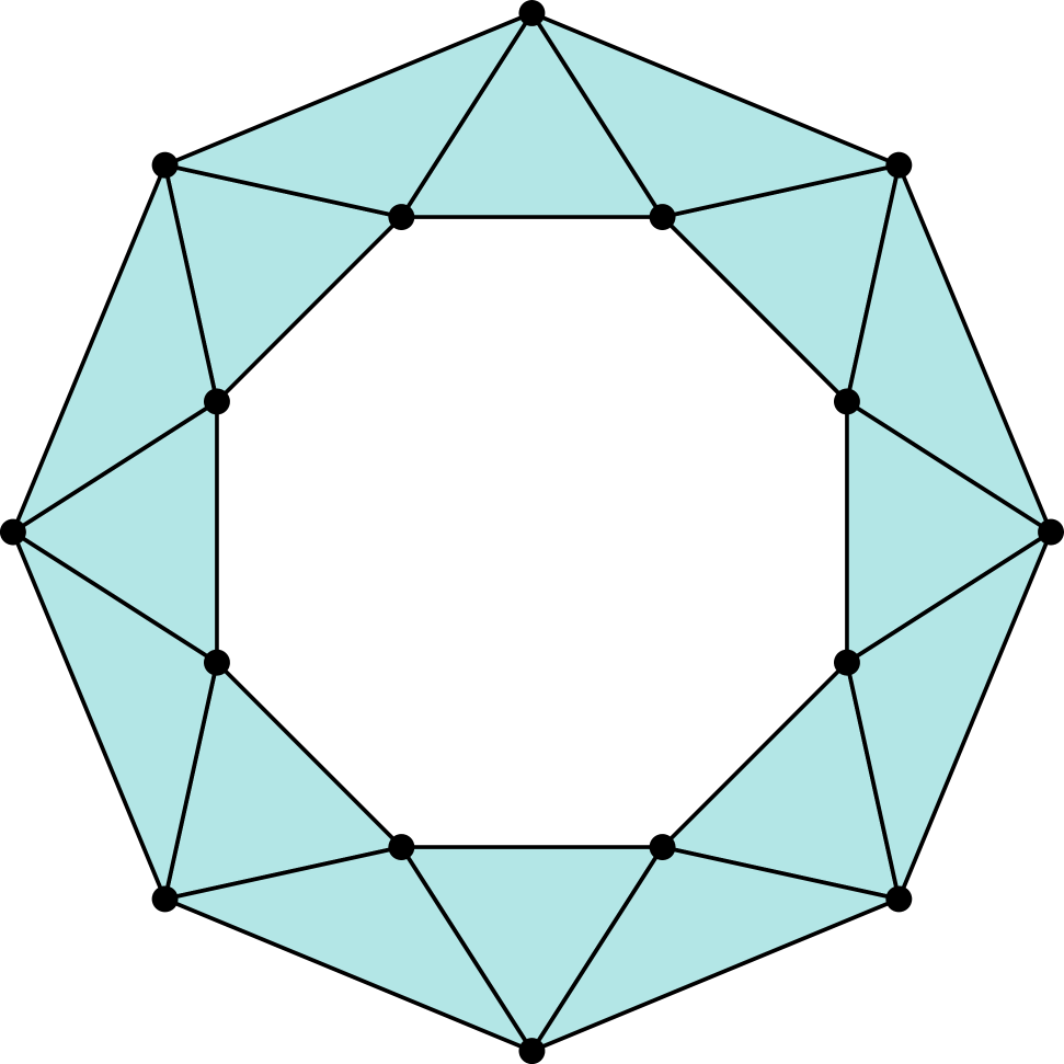
$\begin{gathered}\beta^{0}(X;\mathbb{Z}_{2})=1\\ \beta^{1}(X;\mathbb{Z}_{2})=1\end{gathered}$

$\begin{gathered}\beta^{0}(Y;\mathbb{Z}_{2})=1\\ \beta^{1}(Y;\mathbb{Z}_{2})=1\end{gathered}$

$\begin{gathered}\beta^{0}(Z;\mathbb{Z}_{2})=1\\ \beta^{1}(Z;\mathbb{Z}_{2})=1\end{gathered}$

Figure 1. Three simplicial complexes with identical Betti numbers but different structural properties.

As stated in [34] to explain and motivate the study of persistence: “a hole is a hole no matter how fragile or fine”. However, despite its multiple advantages and applications in various fields, persistent homology, as far as we know, does not provide tools to assess the fragility or fineness of a cycle or hole, nor does it allow analyzing its stability beyond its temporal persistence. Additionally, it does not offer a framework to predict the emergence or disappearance of these cycles.

Our goal is to conduct a robustness study in simplicial networks, focusing on how thick or cohesive a cycle is and how robust or resilient it is against potential failures or attacks the network may suffer. The idea arises from the context of neurodegenerative diseases, where the disconnection or death of neurons, or the loss of synaptic connections, contribute to neuronal dysfunction and, eventually, to the loss of brain tissue. From a mathematical perspective, if a neuronal network is modeled as a simplicial complex, the degenerative process translates into the disappearance of vertices (neurons) or even simplices (connections or synapses among groups of neurons), which can lead to partial or total disconnections between different regions within the cerebral cortex, thus causing significant changes in its topology and functionality. From this perspective, the robustness of a cycle can be evaluated in two stages: its thickness (determined by the dimension of the simplices composing it) and the strength of its connections (defined by the strength of the adjacencies between its simplices).

In this work, we borrow the ideas of persistent homology in TDA to create different filtrations that allow modeling two distinct simplicial elimination rules and we examine their impact on the structure of the simplicial complex. This enables us to introduce two novel families of Betti numbers for finite simplicial complexes that extend the classical invariants by incorporating richer structural information: the thick and the cohesive Betti numbers.

On the one hand, we remove the simplices that are not a face of an $h$-simplex. In this way, the filtration we propose is a cofiltration based on the coskeletons of a simplicial complex, and this construction provides information about the dimensions of the facets defining the holes and connected components of the simplicial complex. This construction allows us to introduce the thick Betti numbers, where the $(n,h)$-thick Betti number can be interpreted as the number of $n$-dimensional holes formed by paths of simplices of dimension $h$ or higher and thus, they capture how thick the links of the cycles are.

On the other hand, we remove the simplices with some fixed dimensions. This provides insights into the interaction of simplices of different dimensions and, therefore, into higher-order adjacencies. The cohesive Betti numbers are then defined, enhancing the information captured by the thick Betti numbers by providing insight into the higher-order adjacencies between the simplices enclosing the holes of the simplicial complex. That is, they assess how strong the connection is among the simplices of the homology cycle. They are more technical to define and sheaf theory over finite topological spaces is needed to analyze how simplices of specific dimensions interact with each other.

Finally, we show that the resilience of topological features to simplicial attacks can be captured using biparameter persistence modules, where one parameter traces the progression of the attack, while the other reflects structural refinements based on cycle thickness or network cohesiveness.

While persistence is traditionally applied to analyze real-world data by tracking homological features across scales, here we repurpose it as a theoretical tool to systematically study the robustness and structural evolution of simplicial complexes under simplices removal.

The main contributions of this article are:

1. The introduction of thick Betti numbers, which refine the classical Betti numbers by incorporating information about the dimension of the simplices defining the connected components and holes. They measure how thick the links of the homology cycle are.

2. The introduction of cohesive Betti numbers, which extend the analysis to higher-order adjacencies between simplices. They assess how strong the connection is among the links of the homology cycle.

3. The application of persistence to the comprehensive study of the robustness of topological features in finite simplicial complexes, using both thick and cohesive Betti numbers.

4. The development of a biparameter persistence framework for modeling topological resilience, where one parameter tracks simplicial attacks and the other encodes structural features related to cycle thickness or network cohesion.

This paper is structured as follows. Section 2 introduces the necessary preliminaries on simplicial complexes, Betti numbers, and persistence –via cofiltrations and simplicial cohomology– as well as on finite topological spaces, which are needed for the development of the paper. In Section 3, we define the thick Betti numbers. Using coskeleta (Definition 3.1), we introduce this new family of invariants for simplicial complexes and prove that they are indeed simplicial invariants (Theorem 3.3). Through the study of the persistence module induced by the coskeletal cofiltration (Section 3.2), we show that thick Betti numbers quantify the thickness of homological holes in terms of the dimension of their surrounding simplices. Section 4 refines the study of robustness in simplicial networks by introducing the cohesive Betti numbers (Definition 4.3), which we also prove to be simplicial invariants (Theorem 4.5). As with thick Betti numbers, cohesive Betti numbers are introduced within a persistent framework (Section 4.2) and serve as indicators of the cohesion of homology cycles, contributing to a deeper understanding of robustness. Finally, Section 5 presents a biparameter persistence approach to analyze the resilience of holes and connected components under simplicial attacks. One parameter encodes the progression of the attack, while the other reflects structural information provided by coskeletal or cohesive cofiltrations.

2. Preliminaries

To start with, we will give a brief overview of some basic notions and facts about simplicial complexes, persistence and finite topological spaces which, in the sequel, will be useful for the convenience of the reader unfamiliar with these subjects. For a thorough exposition we refer to [50, 41] for simplicial complexes, to [23, 20, 35] for persistence and to [22, 5] for finite spaces.

2.1. Simplicial complexes

Let $V$ be a finite set and let ${\mathcal{P}}(V)^{*}$ be the set of non-empty subsets of $V$.

Definition 2.1.

An (abstract) simplicial complex on the ground set $V$ is a subset $X$ of ${\mathcal{P}}(V)^{*}$ closed under taking subsets, that is, if $\sigma\in X$, then ${\mathcal{P}}(\sigma)^{*}\subseteq X$.

The elements $\sigma$ of $X$ are called simplices or faces of $X$ and the elements of $\sigma$ are called vertices. That is, the vertices of $X$ are the one-point sets of $X$. Let us denote by $V(X)$ the set of vertices of $X$. If $\sigma\subseteq\tau$ we also say that $\sigma$ is a face of $\tau$ and we shall put $\sigma{\trianglelefteqslant}\tau$. A maximal face of $X$ (with respect to the inclusion of subsets) is called a facet. Then, a simplicial complex is completely defined by the set of its facets.

(a) Simplices

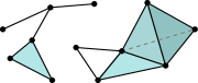
(b) Simplicial complex

Figure 2. We can represent a $0$-simplex as a point, a $1$-simplex as an edge, a $2$-simplex as a filled triangle, a $3$-simplex as a filled tetrahedron, etc. (A), and a simplicial complex as a set of simplices glued together in such a way that the intersection of any two simplices is another simplex (B).

A simplex $\sigma\in X$ consisting of $n+1$ vertices is called an $n$-simplex and we say that it has dimension $n$. The set of $n$-simplices of a simplicial complex $X$ is denoted by $S^{n}(X)$.

The dimension of a simplicial complex $X$ is defined as the maximum of the dimensions of its simplices, $\dim\,X=\max\{\dim\,\sigma:\sigma\in X\}$.

Definition 2.2.

Let $X$ and $Y$ be simplicial complexes with vertex sets $V(X)$ and $V(Y)$ respectively. A simplicial morphism $f\colon X\to Y$ is an application $f\colon V(X)\to V(Y)$ which maps simplices of $X$ into simplices of $Y$ (possibly of smaller dimension). $f\colon X\to Y$ is an isomorphism of simplicial complexes if it is bijective and both $f$ and $f^{-1}$ are simplicial morphisms. In particular, injective morphisms preserve the dimension of the simplices.

As mentioned above (Figure 2), a simplicial complex is constructed by gluing simplices together by means of their faces, resulting in different degrees of adjacency between the simplices. Here we focus on the notion of lower adjacencies introduced in [42].

Definition 2.3.

Let $\tau$ and $\tau^{\prime}$ be simplices of a simplicial complex $X$. We say that $\tau$ and $\tau^{\prime}$ are $h$-lower adjacent if there exist a $h$-simplex $\sigma$ such that $\sigma{\trianglelefteqslant}\tau$ and $\sigma{\trianglelefteqslant}\tau^{\prime}$. In this case, we write $\tau\sim_{L_{h}}\tau^{\prime}$.

Definition 2.4.

Let $X$ be a simplicial complex and let $0\leq h_{0}<h_{1}$.

• An $(h_{0},h_{1})$-walk is a sequence $\{\tau_{1},\tau_{2},\dots,\tau_{r}\}$ of $h_{0}$-lower adjacent simplices such that $h_{1}=\min\{\dim\tau_{i}\}$,

  $$\tau_{1}\sim_{L_{h_{0}}}\tau_{2}\sim_{L_{h_{0}}}\dots\sim_{L_{h_{0}}}\tau_{r}\ \ ,\ \ h_{1}=\min\,\dim\,\tau_{i}$$

  We say that a walk is closed if $\tau_{1}=\tau_{r}$.

• For a pair of simplices $\sigma$ and $\sigma^{\prime}$ we define

  $$\sigma\sim_{h_{0}h_{1}}\sigma^{\prime}\iff\exists\quad(h_{0},h_{1})\text{-walk }\,\{\tau_{1},\tau_{2},\dots,\tau_{r}\}:\sigma{\trianglelefteqslant}\tau_{1}\,\text{ and }\,\sigma^{\prime}{\trianglelefteqslant}\tau_{r}\,.$$ (1)

  In addition, we set that $\sigma\sim_{h_{0}h_{1}}\sigma$ for each $\sigma\in X$.

• We call $(h_{0},h_{1})$-connected components of $X$ the equivalence classes of the quotient set ${S^{h_{0}}(X)}/{\sim_{h_{0}h_{1}}}$.

Example 2.5.

Figure 3 shows a connected simplicial complex with three $(0,2)$-connected components (marked in red). The $(0,2)$-connected components measure the connectivity of the vertices through walks of adjacent triangles.

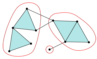
Figure 3. $(0,2)$-connected components.

This connectivity is closely related to the “$q$-connectivity” in [2, 47, 43]. Indeed, the set of $q$-connected components defined in [47] is in bijection with the set of $(q,q+1)$-connected components whose equivalence classes contain more than one element. In particular, the $(0,1)$-connected components are the usual connected components of the simplicial complex.

From here we will always assume that $V$ is a finite ordered set, that is, a set of cardinality, say, $N$ equipped with a bijection map $o\colon\{1,\dots,N\}\to V$. This bijection map is called a total ordering in $V$ and we denote $v_{i}=o(i)$. Then, if $\sigma$ is a $n$-simplex in $X$ with vertices $\{v_{i}\}_{i\in I}$, for some $I\subseteq\{1,\dots,N\}$, we shall denote $\sigma=(v_{i_{0}},\dots,v_{i_{n}})$ being $i_{0}<i_{1}<\cdots<i_{n}$.

Definition 2.6.

Given a simplicial complex $X$ and a field $\Bbbk$, the space of $n$-cochains on $X$, denoted by $C^{n}(X;\Bbbk)$, is the $\Bbbk$-vector space spanned by the set of $n$-simplices of $X$

$$C^{n}(X;\Bbbk)=\displaystyle\prod_{\dim\sigma=n}\Bbbk$$ (2)

Remark 2.7.

Cochains are referred to as topological signals in Topological Deep Learning ([40]).

Once a total ordering has been fixed on the set of vertices of $X$, there exists a coboundary operator

$$\delta^{n}\colon C^{n}(X;\Bbbk)\to C^{n+1}(X;\Bbbk)$$

defined for each $\sigma=(v_{i_{0}},v_{i_{1}},\dots,v_{i_{n+1}})$ such that $i_{0}<i_{1}<\dots<i_{n+1}$ and each $x\in C^{n}(X;\Bbbk)$ as

$$(\delta^{n}\,x)_{\sigma}=\sum_{j=0}^{n+1}(-1)^{i}\,x_{(v_{i_{0}},\dots,\widehat{v_{i_{j}}},\dots,v_{i_{n+1}})}$$ (3)

The notation $\widehat{v_{i_{j}}}$ means that the element ${v_{i_{j}}}$ has been removed.

One can check that these linear maps satisfy $\delta^{n+1}\circ\delta^{n}=0$ for all $n\geq 0$, so $(C^{\bullet}(X;\Bbbk),\delta^{\bullet})$ defines a cochain complex.

Definition 2.8.

The $n$-th simplicial cohomology space with coefficients in $\Bbbk$ of the simplicial complex $X$, is the quotient

$$H^{n}(X;\Bbbk)=\text{Ker}\,\delta^{n}/\text{Im}\,\delta^{n-1}\,.$$

Remark 2.9.

The simplicial cohomology spaces that we have defined do not depend on the total order fixed on the set of vertices. Moreover, the usual definition of simplicial cohomology [32] is based on the cochain spaces and coboundary maps obtained by taking dual in the chain spaces and boundary maps that define the simplicial homology [50]. The definition presented here is equivalent to the usual one, as follows from the linear isomorphisms $C^{n}(X;\Bbbk)\simeq\text{Hom}_{\Bbbk}(C_{n}(X;\Bbbk);\Bbbk)$ which associates to each generator $1_{\sigma}\in\Bbbk_{\sigma}$ the linear map $\omega_{\sigma}\colon C_{n}(X;\Bbbk)\to\Bbbk$ defined for each $\mu\in X$ as

$$w_{\sigma}(1_{\mu})=\begin{cases}1&\text{ if }\mu=\sigma\\ 0&\text{ otherwise}\end{cases}$$

Given a simplicial morphism $f\colon X\to Y$, for each simplex $\sigma=(v_{i_{0}},\dots,v_{i_{n}})$ its image $f(\sigma)$ is a simplex in $Y$, whose dimension could be less than the dimension of $\sigma$. Moreover, even if $f(\sigma)$ is a $n$-simplex, the ordering of its vertices $f(v_{i_{0}}),\dots,f(v_{i_{n}})$ might be not compatible with the ordering given in $Y$. Thus, let us denote by $\epsilon_{\sigma}$ the permutation on the indices $\{0,\dots,n\}$ such that (the indices of) the vertices of $f(\sigma)$ appear according to the ordering in $Y$, that is, and abusing notation, $f(v_{i_{\epsilon(0)}})<\cdots<f(v_{i_{\epsilon(n)}})$. We denote by $\epsilon_{\sigma}\cdot f(\sigma)$ the $n$-simplex $(f(v_{i_{\epsilon(0)}}),\dots,f(v_{i_{\epsilon(n)}}))$. Then, for each $n\geq 0$ there is a linear transformation

$${f^{n}}\colon C^{n}(Y;\Bbbk)\to C^{n}(X;\Bbbk)$$

defined for each $y\in C^{n}(Y;\Bbbk)$ and each $n$-simplex $\sigma=(v_{i_{0}},v_{i_{1}},\dots,v_{i_{n}})\in X$ as

$${f^{n}}(y)_{(v_{i_{0}},v_{i_{1}},\dots,v_{i_{n}})}=\begin{cases}(-1)^{|\epsilon_{\sigma}|}y_{\epsilon_{\sigma}\cdot f(\sigma)}&\text{ if }f(v_{i_{j}})\neq f(v_{i_{k}})\,\forall\,i_{j}\neq i_{k}\\ 0&\text{ otherwise}\end{cases}$$ (4)

Note that $(-1)^{|\epsilon_{\sigma}|}$ denote the sign of $\epsilon_{\sigma}$. These linear maps satisfy ${f^{n+1}}\circ\delta^{n}=\delta^{n}\circ{f^{n}}$, so they induce morphisms between the cohomology spaces

$$\begin{array}[]{rccc}H^{n}(f)\colon&H^{n}(Y;\Bbbk)&\longrightarrow&H^{n}(X;\Bbbk)\\ &[y]&\longmapsto&[{f^{n}}(y)]\end{array}$$

The assignments above are functorial, meaning that they are compatible with identity and composition: $H^{n}(\text{Id})=\text{Id}$ and $H^{n}(g\circ f)=H^{n}(f)\circ H^{n}(g)$.

Definition 2.10.

Given a simplicial complex $X$, a field $\Bbbk$ and $n\geq 0$, the $n$-th Betti number of $X$ with coefficients in $\Bbbk$ is defined as the dimension of the $n$-th simplicial cohomology space associated to $X$ with coefficients in $\Bbbk$,

$$\beta^{n}(X;\Bbbk)=\dim\,H^{n}(X;\Bbbk)\,.$$

Remark 2.11.

Betti numbers of simplicial complexes are usually defined as the dimension of simplicial homology spaces [50] rather than the dimension of simplicial cohomology spaces. However, in our case both definitions agree as follows from the Universal Coefficient Theorem for cohomology ([32, Proposition 12.9]).

Proposition 2.12.

The Betti numbers are simplicial invariants. That is, if $X$ and $Y$ are finite isomorphic simplicial complexes, then $\beta^{n}(X;\Bbbk)=\beta^{n}(Y;\Bbbk)$, for every $n\geq 0$.

Proof.

It follows by the functoriality of the cohomology. ∎

In the sense of the previous proposition, we say that Betti numbers are invariants associated to the category of simplicial complexes, which allow us to distinguish non-isomorphic simplicial complexes. Moreover, Betti numbers give us topological information about the structure of the simplicial complex: $\beta^{0}(X;\Bbbk)$ counts the number of connected components of $X$ and, for $n\geq 1$, $\beta^{n}(X;\Bbbk)$ is usually interpreted as the number of “$n$-dimensional holes” in the simplicial complex.

2.2. Persistence

Persistence is a key concept in Topological Data Analysis, primarily used to study of the “shape” of point clouds [23, 20, 35]. In the standard setting, the starting point is a filtration of simplicial complexes, i.e. a nested sequence of simplicial complexes indexed by some integer or real parameter. Such sequences usually arise when we try to model a point cloud (a finite set of points endowed with a distance) by a simplicial complex, for example using the Vietoris-Rips, Čech or Alpha constructions [20]. The idea behind persistent homology is to track the topological features of the simplicial complexes throughout the filtration by using simplicial homology.

Given the interests of our paper, we will introduce persistence from a dual point of view, by means of cofiltrations and simplicial cohomology.

Definition 2.13.

A cofiltration of simplicial complexes indexed by a partially ordered set $P$ is a family $\{X^{p}\}_{p\in P}$ of simplicial complexes such that $X^{p}\supseteq X^{q}$ for each $p\leq q$.

Example 2.14.

A finite $1$-parameter cofiltration (Figure 4) is a nested sequence of simplicial complexes

$$X^{0}\supseteq X^{1}\supseteq X^{2}\supseteq\dots\supseteq X^{N}$$

This configuration occurs, for instance, when simplices are successively removed from an initial simplicial complex $X^{0}$, modelling an arbitrary degenerative process.

Given a cofiltration of simplicial complexes $\{X^{p}\}_{p\in P}$, the aim is to follow the changes in the topology of the simplicial complexes along the cofiltration. This is performed by studying the vector spaces $H^{n}(X^{p};\Bbbk)$ and the linear maps $\varphi_{pq}\colon H^{n}(X^{p};\Bbbk)\to H^{n}(X^{q};\Bbbk)$ induced by the inclusions $X^{p}\supseteq X^{q}$. The resulting object is known as a persistence module, a notion which appears in [21] motivated by the study of the homology of a filtration.

Definition 2.15.

Let $P$ be a partially ordered set. A persistence module $M$ (indexed by $P$) is a set $\{M_{p}\}_{p\in P}$ of $\Bbbk$-vector spaces together with linear maps $\varphi_{pq}\colon M_{p}\to M_{q}$ for all $p\leq q$, such that $\varphi_{pp}=\text{Id}_{M_{p}}$ and $\varphi_{qr}\circ\varphi_{pq}=\varphi_{pr}$ for all $p\leq q\leq r$ .

A morphism of persistence modules $\Phi\colon M\to N$ is a set of linear maps $\{\Phi_{p}\colon M_{p}\to N_{p}\}_{p\in P}$ such that for each $p\leq q$ the following diagram commutes

If $\Phi_{p}$ is bijective for all $p\in P$, then $\Phi$ is an isomorphism.

We say that the persistence module $M$ is pointwise finite-dimensional if all the spaces $M_{p}$ are finite dimensional.

Example 2.16.

A persistence module $M$ indexed by $\mathbb{N}\times\mathbb{N}$ is a called a biparameter persistence module and consists of a commutative diagram of vector spaces and linear maps of the form:

(5)

Definition 2.17.

Let $I$ be an interval of a totally ordered set $T$, that is, a subset such that if $t\leq s\leq r$ and $t,r\in I$, then $s\in I$ as well. We denote by $\Bbbk[I]$ the persistence module defined, for every $t\in T$ and every $t\leq s$, as

$$\Bbbk[I]_{t}=\begin{cases}\Bbbk&\text{ if }t\in I\\ 0&\text{ otherwise}\end{cases}\ \ \ \text{ and }\ \ \ \varphi_{ts}=\begin{cases}Id_{\Bbbk}&\text{ if }t,s\in I\\ 0&\text{ otherwise}\end{cases}$$

We say that $\Bbbk[I]$ is an interval persistence module and, according to the following structure theorem, they are the basic building blocks to obtain other persistence modules.

Theorem 2.18.

([15, Theorem 1.2]) Every pointwise finite-dimensional persistence module $M$ indexed by a totally ordered set decomposes in an unique way (unique up to reordering) as a direct sum of interval modules, $M\simeq\displaystyle\bigoplus_{\lambda\in\Lambda}\Bbbk[I_{\lambda}]$.

The collection of intervals $\{I_{\lambda}\}_{\lambda\in\Lambda}$ for which $M\simeq\displaystyle\bigoplus_{\lambda\in\Lambda}\Bbbk[I_{\lambda}]$ is known as the persistence barcode of $M$. Various persistent homology software implementations are available for computing persistence barcode (see [53]).

Example 2.19.

Taking the $n$-th simplicial cohomology of a finite $1$-parameter cofiltration of simplicial complexes (Example 2.14) we obtain a persistence module

$$H^{n}(X^{\bullet};\Bbbk)\equiv H^{n}(X^{0};\Bbbk)\to H^{n}(X^{1};\Bbbk)\to\dots\to H^{n}(X^{N};\Bbbk)$$

By Theorem 2.18, it decomposes as a direct sum of intervals of the finite set $\{0,1,\dots,N\}$,

$$H^{n}(X^{\bullet};\Bbbk)\simeq\bigoplus_{i=1}^{m}[b_{i},d_{i})\ \ ,\ \ \text{for some }0\leq b_{i}<d_{i}\leq N+1.$$

The persistence barcode, $\{[b_{i},d_{i})\}_{i=0}^{m}$, is represented as a set of bars over the real line. These bars visually encode the behaviour of the topological features along the cofiltration (Figure 4). Each bar corresponds to an interval during which a cohomology class persists, with $b_{i}$ and $d_{i}$ indicating its birth and death, respectively. In particular, long bars correspond to cohomology classes with high persistence, which are therefore more robust to the deletion of simplices from the initial simplicial complex $X^{0}$.

Example 2.20.

Figure 4 provides an example of a cofiltration indexed by the ordered set $\{0,1,2,3,4,5\}$ and the barcodes of the persistence modules associated with the $0$-th and $1$-st simplicial cohomology with coefficients in $\mathbb{Z}_{2}$. The $H^{0}(X^{\bullet};\mathbb{Z}_{2})$ barcode tracks the connected components of the simplicial complexes. A bar starts at $0$ and reflects the connectivity of the initial simplicial complex. The connectivity is not affected by the first two removals, but it is at step $3$, where one of the vertices is disconnected from the rest, so a new bar appears. This bar persists until step $5$, when the vertex on the right is removed. Also in step $5$, two connected components are born due to the elimination of the remaining edges. As for the $1$-dimensional holes captured by $H^{1}(X^{\bullet};\mathbb{Z}_{2})$, there are two bars in the corresponding barcode. Both bars start at step $1$, when two holes are “born” due to the removal of the interior of the triangles from the initial simplicial complex. One of them “dies” immediately in step $2$ but the other persists until step $4$, as shown by the top bar.

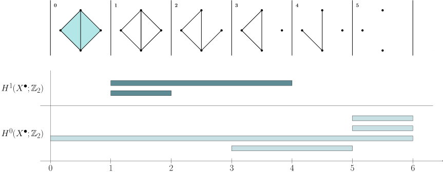
Figure 4. Cofiltration of a simplicial complex and the barcodes of the persistence modules associated with the $0$-th and $1$-st simplicial cohomology with coefficients in $\mathbb{Z}_{2}$.

Remark 2.21.

Unlike the single-parameter case, the analysis of multi-parameter persistence modules presents several challenges [16]. A key difficulty is that there is no straightforward generalization of the barcode decomposition theorem (Theorem 2.18). Several invariants have been proposed in TDA for multiparameter persistence, such as the Hilbert function, the rank invariant or the bigraded Betti numbers. Moreover, persistence barcodes may be obtained from a biparameter persistence module $M_{(\bullet,\bullet)}$ by restricting it to single-persistence modules defined by totally ordered subsets of $\mathbb{N}\times\mathbb{N}$, such as the vertical or the horizontal lines of diagram (5). To facilitate the computation and visualization of these invariants, software tools such as RIVET [61, 45] have been developed.

2.3. Finite topological spaces

Simplicial cohomology of finite simplicial complexes can be understood from the point of view of sheaf theory ([17, 32]) over finite topological spaces, as we will see in this section. This approach will be useful in the definition of the cohesive Betti numbers in Section 4.

To begin with, we recall the relationship between finite topological spaces and finite posets, [49].

Every finite poset $P$ can be though as a topological space endowing it with the Alexandrov topology, whose open sets are the upper sets of $P$. That is, $U\subseteq P$ is open if and only if for every $p\in U$ and every $q\in P$ such that $p\leq q$ it follows that $q\in U$. In particular, given $p\in P$, the open set $U_{p}\coloneqq\{q\in P:p\leq q\}$ is the minimal open set of $P$ that contains $p$.

Conversely, given a finite topological space $X$, we can define a preorder on its set of points as $p\leq q$ if $U_{q}\subseteq U_{p}$, where $U_{p}$ denotes the minimum open set containing $p$. In particular, if $X$ is a $T_{0}$ space, the defined preorder is a partial order.

Theorem 2.22.

The above assignments are functorial and define an equivalence between the category of finite $T_{0}$ topological spaces and the category of finite posets.

Proof.

The assignments are mutually inverse. Moreover, a map $f\colon P\to Q$ between finite posets is monotone ($p\leq p^{\prime}\Rightarrow f(p)\leq f(p^{\prime})$) if and only if it is continuous for the corresponding topologies. The details can be found in [5]. ∎

Thus, given a poset $P$ and a field $\Bbbk$, we can compute the sheaf cohomology spaces associated to the constant sheaf $\Bbbk$ over $P$, viewing $P$ as a topological space by means of the equivalence given by the above Theorem. To compute $H^{n}(P,\Bbbk)$ we can make use of the standard resolution of the constant sheaf [56]. Taking its global sections yields a cochain complex consisting of the vector spaces

$$C^{n}(P;\Bbbk)\coloneqq\!\!\!\displaystyle\prod_{(p_{0}<p_{1}<\dots<p_{n})\in P}\!\!\!\Bbbk$$ (6)

and the coboundary morphisms $\delta^{n}\colon C^{n}(P;\Bbbk)\to C^{n+1}(P;\Bbbk)$, defined for each $x\in C^{n}(P;\Bbbk)$ and each $(p_{0}<p_{1}<\dots<p_{n+1})\in P$ as

$$(\delta^{n}x)_{p_{0}<p_{1}<\dots<p_{n+1}}\coloneqq\sum_{i=0}^{n}(-1)^{i}x_{p_{0}<\dots<\widehat{p_{i}}<\dots<p_{n+1}}$$ (7)

These linear transformations satisfy $\delta^{n+1}\circ\delta^{n}=0$ and $H^{n}(P;\Bbbk)\simeq{\text{Ker}\,\delta^{n}}/{\text{Im}\,\delta^{n-1}}$, for all $n\geq 0$.

The sheaf cohomology of the constant sheaf $\Bbbk$ is functorial: given a continuous map between finite spaces $f\colon P\to Q$, for each $n\geq 0$ there is a linear map

$$f^{n}\colon C^{n}(Q;\Bbbk)\longrightarrow C^{n}(P;\Bbbk)$$

defined for each $y\in C^{n}(Q;\Bbbk)$ and each $p_{0}<p_{1}<\dots<p_{n}\in P$ as

$$f^{n}(y)_{p_{0}<p_{1}<\dots<p_{n}}=\begin{cases}y_{f(p_{0})<f(p_{1})<\cdots<f(p_{n})}&\text{ if }f(p_{i})\neq f(p_{i+1})\ \forall\,0\leq i\leq n-1\\ 0&\text{otherwise}\end{cases}$$

This map induces a linear map in cohomology

$$\begin{array}[]{rccc}H^{n}(f)\colon&H^{n}(Q;\Bbbk)&\longrightarrow&H^{n}(P;\Bbbk)\\ &[y]&\longmapsto&[{f^{n}}(y)]\end{array}$$

satisfying that $H^{n}(Id)=Id$ and $H^{n}(f\circ g)=H^{n}(g)\circ H^{n}(f)$.

Definition 2.23.

The face poset of a simplicial complex $X$, denoted by $P_{X}$, is the set of simplices of $X$ equipped with the partial order given by the face relation ${\trianglelefteqslant}$.

Theorem 2.24.

The $n$-th simplicial cohomology with coefficients in $\Bbbk$ of a simplicial complex $X$ is isomorphic to the sheaf cohomology of the constant sheaf $\Bbbk$ over its face poset $P_{X}$,

$$H^{n}(X;\Bbbk)\simeq H^{n}(P_{X};\Bbbk)$$

Proof.

It follows from [32, Theorem 13.18], by viewing the simplicial cohomology as the Čech cohomology of the constant sheaf $\Bbbk$ over $P_{X}$. ∎

Corollary 2.25.

The Betti numbers of a simplicial complex $X$ can be computed via sheaf cohomology as

$$\beta^{n}(X;\Bbbk)=\dim H^{n}(P_{X};\Bbbk)$$

3. How thick is a hole?

In this section, we will use coskeletons and persistence to introduce a collection of new invariants associated to (the category of) simplicial complexes: the thick Betti numbers. As we shall see, these invariants reveal structural properties of the cohomological cycles of a simplicial complex related to the dimension of their constituting simplices, providing us a way to quantify the robustness of a simplicial network in terms of the thickness of its connected components and holes.

3.1. Thick Betti numbers

Definition 3.1.

Given a simplicial complex $X$ and $h\in\mathbb{Z}_{\geq 0}$, the $h$-coskeleton of $X$ is defined as

$$X^{h}=\{\sigma\in X:\exists\,\tau\in X\,\text{ with }\,\sigma{\trianglelefteqslant}\tau\,\text{ and }\dim\tau\geq h\}\,.$$

The $h$-coskeleton is a simplicial subcomplex of $X$ and, in contrast to the $h$-skeleton of a simplicial complex (consisting of the simplices of dimension less than or equal to $h$), it considers the simplices of dimension greater than or equal to $h$ together with all their faces (Figure 5). In other words, the $1$-coskeleton removes all vertices that do not belong to any edge, the $2$-coskeleton removes all vertices and edges that are not part of any filled triangle, and so on. The resulting subcomplex, $X^{h}$, highlights the topological features of $X$ defined by higher dimensional facets (those with dimension $\geq h$). Additionally, we gain insight into the relevance of smaller facets by analysing the effect of their removal on the structure of the complex.

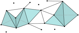
(a) Simplicial complex $X$

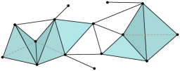
(b) $1$-coskeleton $X^{1}$

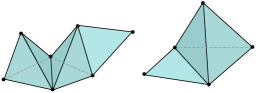
(c) $2$-coskeleton $X^{2}$

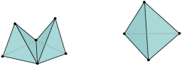
(d) $3$-coskeleton $X^{3}$

Figure 5. We can recursively obtain the $h$-coskeleton by eliminating from the $(h-1)$-coskeleton the simplices that are not a face of an $h$-simplex.

Definition 3.2.

The $(n,h)$-th thick Betti number of a simplicial complex $X$ with coefficients in $\Bbbk$ is the dimension of the $n$-th simplicial cohomology space with coefficients in $\Bbbk$ of the $h$-coskeleton of $X$, that is:

$$\beta^{n,h}(X;\Bbbk)=\dim H^{n}(X^{h};\Bbbk)\,.$$

The $(n,h)$-th thick Betti number can be interpreted as the number of $n$-dimensional cycles which are surrounded by simplices of dimension at least $h$. In particular, $\beta^{n,0}(X;\Bbbk)=\beta^{n}(X;\Bbbk)$ for all $n\geq 0$, so the set of thick Betti numbers extends the set of Betti numbers.

Theorem 3.3.

The thick Betti numbers are simplicial invariants. That is, if $X$ and $Y$ are isomorphic simplicial complexes, then $\beta^{n,h}(X;\Bbbk)=\beta^{n,h}(Y;\Bbbk)$ for all $n,h\geq 0$.

Proof.

Every simplicial isomorphism $f\colon X\stackrel{{\scriptstyle\sim}}{{\to}}Y$ restricts to an isomorphism between the $h$-coskeletons, $f^{h}\colon X^{h}\stackrel{{\scriptstyle\sim}}{{\to}}Y^{h}$. By Proposition 2.12 one gets $\dim H^{n}(X^{h};\Bbbk)=\dim H^{n}(Y^{h};\Bbbk)$, for all $n\geq 0$. ∎

Example 3.4.

In Figure 6A, we have a $1$-dimensional hole in $X$ (empty triangle, $\beta^{1}(X)=1$) that is fully enclosed by filled triangles ($2$-simplices). Taking the $2$-coskeleton of $X$ does not alter $X$, and the $(1,2)$-thick Betti number, $\beta^{1,2}(X)=1$, confirms that the hole persists as shown in (B). In (C), the $1$-dimensional hole in $Y$ (empty triangle, $\beta^{1}(Y)=1$) is not completely surrounded by filled triangles, causing the hole to disappear when taking the $2$-coskeleton. This is captured by the thick Betti number, $\beta^{1,2}(Y)=0$, as shown in (D).

Therefore, one can say that the hole in $X$ is thicker than the hole in $Y$, as it is fully enclosed by $2$-simplices.

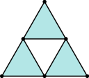
(e) $\beta^{1}(X;\mathbb{Z}_{2})=1$

$$\stackrel{{\scriptstyle h=2}}{{\scalebox{2.2}[1.0]{$\longmapsto$}}}$$

(f) $\beta^{1,2}(X;\mathbb{Z}_{2})=1$

(g) $\beta^{1}(Y;\mathbb{Z}_{2})=1$

$$\stackrel{{\scriptstyle h=2}}{{\scalebox{2.2}[1.0]{$\longmapsto$}}}$$

(h) $\beta^{1,2}(Y;\mathbb{Z}_{2})=0$

Figure 6. Thickness of a hole: a $1$-dimensional hole fully enclosed by $2$-simplices in (A) and a $1$-dimensional hole not surrounded by $2$-simplices in (C). Structural difference is captured by considering $2$-coskeletons: the hole does not change in $X$, figure (B), whereas the hole in $Y$ disappears, figure (D).

For a preliminary definition, we will consider a $n$-dimensional cycle to be thicker than other if it is enclosed by higher dimensional simplices. However, as we will explore in the next section, this requires a more formal treatment.

The following proposition shows that the $(0,h)$-th thick Betti numbers counts the number of connected components which are defined by lower adjacent $h$-dimensional simplices (see Figure 7).

$\beta^{0,2}(X;\mathbb{Z}_{2})=4$

$\beta^{0,2}(Y;\mathbb{Z}_{2})=1$

Figure 7. Two connected simplicial complexes. The $(0,2)$-th thick Betti numbers measure the connectivity between the triangles.

Proposition 3.5.

For any $h>0$ and any field $\Bbbk$, the following formula holds:

$$\beta^{0,h}(X;\Bbbk)=\#\faktor{V(X)}{\sim_{0h}}-\#\{v\in V(X):v\centernot{\lhd}\sigma\textup{ for all }\sigma\in S^{h}(X)\}\,,$$

or, equivalently,

$$\beta^{0,h}(X;\Bbbk)=\#\faktor{S^{\geq h}(X)}{\sim_{0h}}\,,$$

where $S^{\geq h}(X)$ denotes the set of simplices of $X$ of dimension at least $h$.

Proof.

$\beta^{0,h}(X;\Bbbk)$ is the number of connected components of $X^{h}$. That is,

$$\beta^{0,h}(X;\Bbbk)=\#\faktor{V(X^{h})}{\sim_{01}}$$

Given a walk $\{e_{1},e_{2},\dots,e_{r}\}$ of $0$-lower adjacent $1$-simplices of $X^{h}$, by definition of the $h$-coskeleton, there exists a $(0,h)$-walk $\{\sigma_{1},\sigma_{2},\dots,\sigma_{r}\}$ in $X^{h}$ such that $e_{i}{\trianglelefteqslant}\sigma_{i}$ for each $i$. Consequently,

$$\#\faktor{V(X^{h})}{\sim_{01}}=\#\faktor{V(X^{h})}{\sim_{0h}}$$

Finally, the equivalence classes of the last quotient set corresponds to the non-singleton equivalence classes of $V(X)/\sim_{0h}$, which yields the first formula in the proposition.

To prove the second formula, it suffices to observe that there is a bijection between the set of equivalence classes in $V(X)/\sim_{0h}$ consisting of more than one element, and the quotient set $S^{\geq h}(X)/\sim_{0h}$. Indeed, each equivalence class $[v]$ in the former corresponds to the equivalence class of an $h$-simplex containing $v$, and conversely, each class $[\sigma]\in S^{\geq h}(X)/\sim_{0h}$ corresponds to $[v]$ for any vertex $v\in\sigma$. ∎

3.2. Persistence of a hole’s thickness.

Now we would like to answer the following question: how robust or resilient is a hole under the simplicial elimination rule defined by taking coskeletons?

We mentioned earlier that a hole could be considered thicker than another if it was enclosed by higher-dimensional simplices. However, as illustrated in Figure 6, thick Betti numbers do not provide a static way to verify this but instead require a dynamic perspective. It is through the successive simplicial removals that we can determine whether a “thick” hole remains or disappears. This is exactly what the persistence telescope helps us achieve.

The coskeletons of a simplicial complex $X$ give rise to a cofiltration:

$$X=X^{0}\supseteq X^{1}\supseteq X^{2}\supseteq\dots\supseteq X^{N}\supseteq X^{N+1}=\emptyset\ \ ,\ N=\dim X$$

Taking cohomology in degree $n\geq 0$ in the previous cofiltration, we obtain a sequence of $\Bbbk$-vector spaces and linear maps:

$$H^{n}(X^{0};\Bbbk)\to H^{n}(X^{1};\Bbbk)\to\dots\to H^{n}(X^{N-1};\Bbbk)\to H^{n}(X^{N};\Bbbk)\to 0$$ (8)

In short, by simplicial cohomology functoriality, the coskeletons induce for each $n\geq 0$ a persistence module $H^{n}(X^{\bullet};\Bbbk)$ which captures how cohomology classes evolve along the cofiltration.

In particular, since $X^{0}=X$, we can analyze the structure of connected components and holes in $X$ by tracking their persistence as successive coskeletons are taken. This provides a robustness measure for the holes in a simplicial complex: the cohomology classes in $H^{n}(X;\Bbbk)$ with longer persistence correspond to those defined by higher-dimensional facets, meaning they are thicker.

Remark 3.6.

It is also worth noting that if we intend to rigorously analyze other events occurring throughout the coskeletal cofiltration, such as the appearance of holes or connected components, persistence provides the most appropriate framework for this study, as shown in Figure 8) (birth of a thick hole) or illustrate in Example 3.7 (splitting in new connected components).

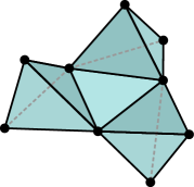
(a) $\beta^{1}(X;\mathbb{Z}_{2})=0$

$$\stackrel{{\scriptstyle h=3}}{{\scalebox{2.2}[1.0]{$\longmapsto$}}}$$

(b) $\beta^{1,3}(X;\mathbb{Z}_{2})=1$

Figure 8. Example of the birth of a hole in the coskeletal cofiltration.

Example 3.7.

The simplicial complex in Figure 9A has two connected components, the same as its non-trivial coskeletons. However, when we take the $2$-coskeleton (Figure 9B), one connected component disappears and the other one is split in two. So, although the Betti numbers remain constant along the coskeletons cofiltration, there may be structural changes when taking successive coskeletons. In (C), the barcode of the persistence module $H^{0}(X^{\bullet};\mathbb{Z}_{2})$ allow us to capture these changes: when $h$ reaches $2$, a bar in the barcode dies (corresponding with the top connected component) and another bar is born (the bottom component splits).

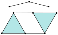
(a) $\beta^{0}(X;\mathbb{Z}_{2})=2$

(b) $\beta^{0,2}(X;\mathbb{Z}_{2})=2$

(c) $H^{0}$ persistence barcode

Figure 9. While the static thick Betti numbers in (A) and (B) indicate the same number of connected components, persistence distinguishes them, as reflected in the barcode of (C).

Theorem 3.8.

Every simplicial isomorphism $X\simeq Y$ induces an isomorphism of persistence modules $H^{n}(X^{\bullet};\Bbbk)\simeq H^{n}(Y^{\bullet};\Bbbk)$, for any $n\geq 0$.

Proof.

Let $f\colon X\stackrel{{\scriptstyle\sim}}{{\to}}Y$ be a simplicial isomorphism. For each $h\geq 0$, $f$ restricts to an isomorphism $f^{h}\colon X^{h}\stackrel{{\scriptstyle\sim}}{{\to}}Y^{h}$. Moreover, for each $h\leq h^{\prime}$, these isomorphisms make the following diagram commutative:

Taking simplicial cohomology, we obtain a commutative diagram:

This establishes the desired isomorphism between $H^{n}(X^{\bullet};\Bbbk)$ and $H^{n}(Y^{\bullet};\Bbbk)$. ∎

We now analyze the birth and death of thick holes, a phenomenon that is captured by the decomposition of the persistence module and is visualized through barcodes. Following Theorem 2.18, the persistence module $H^{n}(X^{\bullet};\Bbbk)$ decomposes into interval modules

$$H^{n}(X^{\bullet};\Bbbk)\simeq\bigoplus_{i=1}^{m}\Bbbk[b_{i},d_{i})\,\text{ with }\,b_{i},d_{i}\in\mathbb{Z}_{\geq 0}\,\text{ and }\,b_{i}<d_{i}\leq\dim\,X+1$$ (9)

Definition 3.9.

Given a simplicial complex $X$, $n\geq 0$ and $0\leq b<d$, we define the $(n,b,d)$-th thick Betti number of $X$ with coefficients in $\Bbbk$, and we denote it $\beta^{n}_{b,d}(X;\Bbbk)$, as the number of intervals of the persistence barcode associated to $H^{n}(X^{\bullet};\Bbbk)$ of the form $[b,d)$. That is, if $H^{n}(X^{\bullet};\Bbbk)\simeq\displaystyle\bigoplus_{i=1}^{m}\Bbbk[b_{i},d_{i})$, then

$$\beta^{n}_{b,d}(X;\Bbbk)=\#\{[b_{i},d_{i}):b_{i}=b\ \text{and}\ d_{i}=d\}_{1\leq i\leq m}$$

The $(n,b,d)$-th thick Betti number of $X$ counts the $n$-dimensional holes formed by removing simplices not contained in those of dimension $\geq b$, which are surrounded by $(d-1)$-simplices but not fully enclosed by $d$-simplices.

Corollary 3.10.

The $(n,b,d)$-thick Betti numbers are simplicial invariants. That is, if $X$ and $Y$ are isomorphic simplicial complexes, then $\beta^{n}_{b,d}(X;\Bbbk)=\beta^{n}_{b,d}(Y;\Bbbk)$ for all $n\geq 0$ and $0\leq b<d$.

Proof.

It is a straightforward consequence of Theorem 3.8 and the uniqueness of the interval decomposition in Theorem 2.18. ∎

The following proposition provides information on the potential birth and death values in the barcode of $H^{n}(X^{\bullet};\Bbbk)$: it shows that equivalence classes in $H^{n}(X^{\bullet};\Bbbk)$ are born either at $h=0$ or at $h\geq n+2$ and that if $H^{n}(X;\Bbbk)$ has a non-trivial equivalence class, it cannot die until $h=n+1$. This corresponds with the intuition that we cannot create new $n$-dimensional holes until we remove $n+1$-dimensional simplices and that we cannot break $n$-dimensional holes until we remove the $n$-dimensional simplices.

Proposition 3.11.

If $h\leq n$, the linear map $H^{n}(X;\Bbbk)\longrightarrow H^{n}(X^{h};\Bbbk)$ induced by the inclusion $X^{h}\subseteq X$ is the identity map. Moreover, the induced morphism $H^{n}(X;\Bbbk)\longrightarrow H^{n}(X^{n+1};\Bbbk)$ is surjective.

Proof.

On the one hand, $H^{n}(X^{h};\Bbbk)$ is defined by the coboundary maps

$$C^{n-1}(X^{h};\Bbbk)\stackrel{{\scriptstyle\delta^{n-1}}}{{\longrightarrow}}C^{n}(X^{h};\Bbbk)\stackrel{{\scriptstyle\delta^{n}}}{{\longrightarrow}}C^{n+1}(X^{h+1};\Bbbk)$$ (10)

On the other hand, $H^{n}(X;\Bbbk)$ is defined by the coboundary maps

$$C^{n-1}(X;\Bbbk)\stackrel{{\scriptstyle\delta^{n-1}}}{{\longrightarrow}}C^{n}(X;\Bbbk)\stackrel{{\scriptstyle\delta^{n}}}{{\longrightarrow}}C^{n+1}(X;\Bbbk)$$ (11)

By definition, the sequences (10) and (11) agree when $h<n$, so $H^{n}(X^{h};\Bbbk)\to H^{n}(X;\Bbbk)$ is the identity. In the case $h=n$, the natural inclusion $i\colon X^{n}\hookrightarrow X$ induces a commutative diagram (Equation (4)):

Moreover, $\delta^{n-1}\colon C^{n-1}(X;\Bbbk)\longrightarrow C^{n}(X;\Bbbk)$ vanishes on the subspace $C^{n-1}(X;\Bbbk)\smallsetminus C^{n-1}(X^{n};\Bbbk)$. Therefore, $\text{Im}\,\delta^{h-1}_{X}=\text{Im}\,\delta^{h-1}_{X^{n}}$ and hence $H^{n}(X;\Bbbk)=H^{n}(X^{n};\Bbbk)$, being $H^{n}(i)$ the identity map.

For the second part of the proposition, we have the commutative diagram:

Where the linear map ${i^{n}}$ is surjective and ${i^{n+1}}$ is the identity map. Thus, given $[x]\in H^{n}(X^{n+1};\Bbbk)$ and taking any $y\in({i^{n}})^{-1}(x)$, by the commutativity of the second square, it verifies that $y\in\text{Ker}\,\delta^{n}$ and $H^{n}(i)([y])=[{i^{n}}(y)]=[x]$. Then, we conclude that the induced morphism $H^{n}(i)\colon H^{n}(X;\Bbbk)\longrightarrow H^{n}(X^{n+1};\Bbbk)$ is surjective. ∎

Corollary 3.12.

The possible non-trivial $(n,b,d)$-th thick Betti numbers are those for which $b=0$ and $d\geq n+1$ or $d>b\geq n+2$.

Focusing on the first case of the previous corollary, $\beta^{n}_{0,d}(X;\Bbbk)$ corresponds to the number of $n$-dimensional holes in $X$ with the minimum dimension of its defining facets being $d-1$. In particular, as the following corollary states, this gives us a stratification of the holes in $X$ relative to the dimension of the simplices defining them (Figure 10).

Corollary 3.13.

Let $X$ be a simplicial complex. Then $\beta^{n}_{0,d}(X;\Bbbk)=0$ for all $d\leq n$ and

$$\beta^{n}(X;\Bbbk)=\sum_{d=n+1}^{\dim X+1}\beta^{n}_{0,d}(X;\Bbbk)\,.$$ (12)

Example 3.14.

Consider the simplicial complex $X$ in Figure 10A, which has two holes ($\beta^{1}(X;\mathbb{Z}_{2})=2$). Figure 10B shows, in yellow and pink, two representatives of independent cohomology classes in $H^{1}(X;\mathbb{Z}_{2})$. Only the yellow one survives the elimination of the middle edge when taking the $2$-coskeleton. This is encoded in the persistence barcode (Figure 10D), from which we obtain $\beta^{1}_{0,2}(X;\mathbb{Z}_{2})=1$ (the minimum dimension of the facets defining the cycle in pink is $1$) and $\beta^{1}_{0,3}(X;\mathbb{Z}_{2})=1$ (the yellow hole is surrounded by triangles). However, it is important to note that this stratification cannot be achieved by analysing the dimension of the facets containing the representatives of cohomology classes defining a basis of $H^{n}(X;\Bbbk)$. For example, the yellow and pink cycles in figure (C) also form a basis of $H^{1}(X;\mathbb{Z}_{2})$ but both include an edge which is not contained in a triangle.

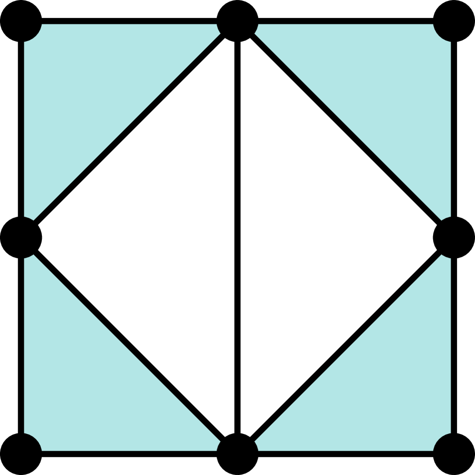
(a)

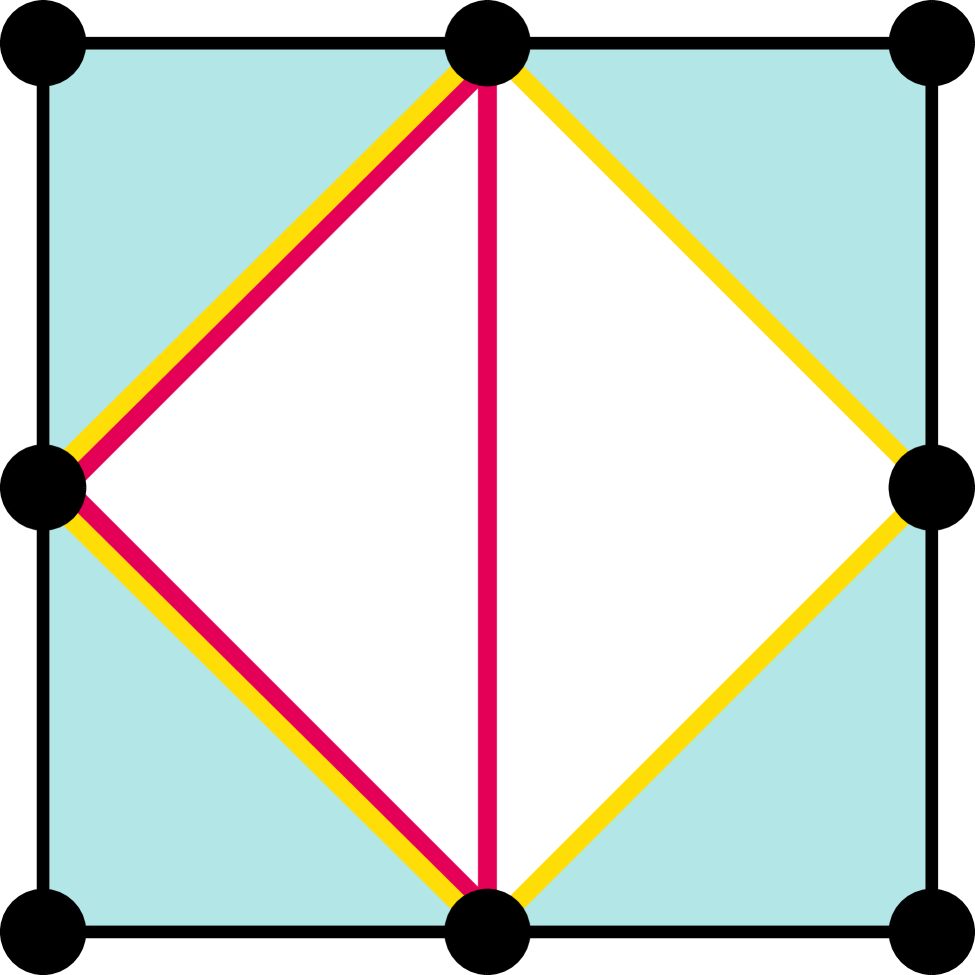
(b)

(c)

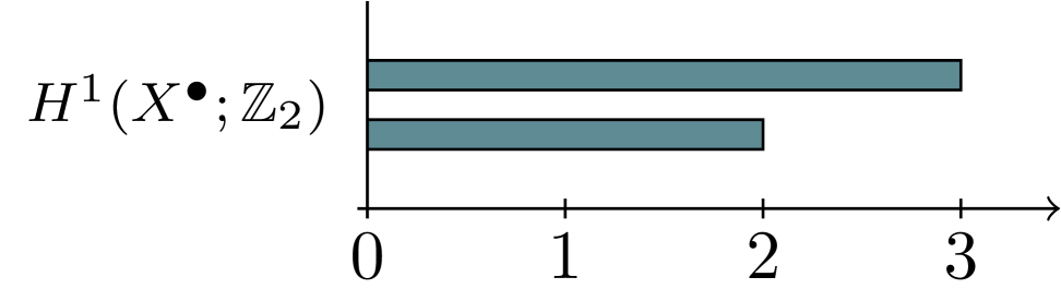
(d)

Figure 10. Simplicial complex (A), representatives of a basis of $H^{1}(X;\mathbb{Z}_{2})$ in yellow and pink (B and C) and thickness persistence barcode (D).

4. How cohesive is a thick hole?

As discussed in the introduction, analyzing the robustness of a simplicial network involves two steps: measuring cycle thickness (using the thick Betti numbers introduced in the previous section) and evaluating the strength of their internal connections, measured by the adjacency between them. Here, we focus on the second aspect.

4.1. Cohesive Betti numbers

Our goal is to analyze the topological impact of removing simplices of fixed dimensions from a simplicial complex. However, the resulting structure is not necessarily a simplicial complex. Imagine a $2$-simplex with its interior removed. The result is a triangle, which can be seen as a graph and thus a 1-dimensional simplicial complex. If, instead, we remove from the $2$-simplex one of its edges, we obtain a hypergraph. However, if we remove its vertices, the resulting structure is neither a simplicial complex nor a hypergraph, but rather a finite space (Section 2.3). Finite spaces thus provide a suitable general framework for analyzing such cases.

In this section, we use sheaf cohomology over finite spaces to introduce a new set of invariants that give us information about the cohesion of cohomological cycles in a simplicial complex. This phenomenon is illustrated in Figure 11, eliminating the vertices separates the triangles on the left while leaving the ones on the right still connected.

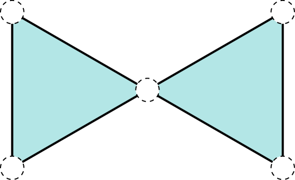
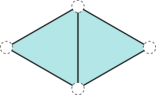
Figure 11. Removing vertices from a simplicial complex.

The dimensions of the simplices of a simplicial complex $X$ define a stratification of the points in the poset $P_{X}$, as shown in its Hasse diagram (Figure 12A).

Definition 4.1.

Let $\mathbf{h}=\{h_{0},h_{1},\dots,h_{m}\}$ be a set of integer numbers such that $0\leq h_{0}<h_{1}<\dots<h_{m}$. We define the $\mathbf{h}$-face poset of $X$, and denote it by $P_{X}^{\mathbf{h}}$, as the subposet defined by the strata of $P_{X}$ corresponding to the dimensions $\{h_{0},h_{1},\dots,h_{m}\}$. That is,

$$P_{X}^{\mathbf{h}}=\{\sigma\in P_{X}:\dim\,\sigma=h_{i}\,\text{ for some }0\leq i\leq m\}.$$

Example 4.2.

Consider the simplicial complex in Figure 6A. In Figure 12A, we present the Hasse diagram of its associated face poset, where the triangles, edges and vertices from Figure 6A correspond to $2$-dimensional, $1$-dimensional, and $0$-dimensional vertices, respectively, in the Hasse diagram. Figure 12B represents its associated $\{0,2\}$-face poset.

(a) $P_{X}$

(b) $P_{X}^{\{0,2\}}$

Figure 12. Hasse diagrams of the face poset (A) of the simplicial complex in Figure 6A and its $\{0,2\}$-face poset (B).

Definition 4.3.

The $(n,\mathbf{h})$-th cohesive Betti number of a simplicial complex $X$ with coefficients in $\Bbbk$ is defined as the dimension of the $n$-th cohomology space of the constant sheaf $\Bbbk$ over the $\mathbf{h}$-face poset,

$$\beta^{n,\mathbf{h}}(X;\Bbbk)=\dim\,H^{n}(P_{X}^{\mathbf{h}};\Bbbk)\,.$$

Taking $\mathbf{h}=\{0,1,\dots,\dim X\}$ one recovers the usual Betti numbers of the simplicial complex, i.e. $\beta^{n,\mathbf{h}}(X;\Bbbk)=\beta^{n}(X;\Bbbk)$ (by Corollary 2.25). Thus, like the thick Betti numbers, the set of cohesive Betti numbers of $X$ extends the set of ordinary Betti numbers.

Remark 4.4.

Notice that $(\beta^{0,\{0\}}(X;\Bbbk),\,\beta^{0,\{1\}}(X;\Bbbk),\,\dots,\,\beta^{0,\{\dim X\}}(X;\Bbbk))$ is the so-called $f$-vector of $X$ and $(\beta^{0,\{0,1,\dots,\dim X\}}(X;\Bbbk),\,\beta^{1,\{0,1,\dots,\dim X\}}(X;\Bbbk),\,\dots,\,\beta^{\dim X,\{0,1,\dots,\dim X\}}(X;\Bbbk))$ is the $\beta$-vector of $X$.

Theorem 4.5.

The cohesive Betti numbers are invariant under simplicial isomorphism. That is, if $X$ and $Y$ are isomorphic simplicial complexes, then $\beta^{n,\mathbf{h}}(X;\Bbbk)=\beta^{n,\mathbf{h}}(Y;\Bbbk)$ for all $n\geq 0$ and all $\mathbf{h}=\{h_{0},h_{1},\dots,h_{m}\}$ such that $0\leq h_{0}<h_{1}<\dots<h_{m}$.

Proof.

Any a simplicial isomorphism $f\colon X\stackrel{{\scriptstyle\sim}}{{\to}}Y$ induces an isomorphism between the face posets, $P_{f}\colon P_{X}\to P_{Y}$ defined for each point $\sigma\in P_{X}$ by $P_{f}(\sigma)\coloneqq f(\sigma)$. Restricting $P_{f}$ to $P_{X}^{\mathbf{h}}$ we obtain an isomorphism between $P_{X}^{\mathbf{h}}$ and $P_{Y}^{\mathbf{h}}$. Then, it follows from the functoriality of sheaf cohomology of the constant sheaf that $H^{n}(P_{X}^{\mathbf{h}};\Bbbk)\simeq H^{n}(P_{Y}^{\mathbf{h}};\Bbbk)$ for all $n\geq 0$. ∎

To understand the information given by this set of new invariants, let us consider, for each $0\leq h_{0}<h_{1}$ and each simplicial complex $X$, the following vector space

$$\Gamma^{h_{0},h_{1}}(X;\Bbbk)\coloneqq\{x\in\prod_{\begin{subarray}{c}\sigma\in X\\ \dim\,\sigma=h_{0}\end{subarray}}\Bbbk\ :\ x_{\sigma}=x_{\sigma^{\prime}}\ \,\forall\,\sigma,\sigma^{\prime}{\trianglelefteqslant}\tau\in X:\dim\tau\geq h_{1}\}$$

Proposition 4.6.

The $\Bbbk$-vector spaces $\Gamma^{h_{0},h_{1}}(X;\Bbbk)$ and $H^{0}(P_{X}^{\mathbf{h}};\Bbbk)$ are isomorphic for any $\mathbf{h}=\{h_{0},h_{1},\dots,h_{m}\}$.

Proof.

The $0$-th cohomology space $H^{0}(P_{X}^{\mathbf{h}};\Bbbk)$ is defined as the kernel of the coboundary map $\delta^{0}\colon C^{0}(P_{X}^{\mathbf{h}};\Bbbk)\to C^{1}(P_{X}^{\mathbf{h}};\Bbbk)$. Then,

$$H^{0}(P_{X}^{\mathbf{h}};\Bbbk)=\{x\in\prod_{\begin{subarray}{c}\sigma\in X\\ \dim\,\sigma\in\mathbf{h}\end{subarray}}\Bbbk\ :x_{\sigma}=x_{\tau}\ \ \forall\,\sigma{\trianglelefteqslant}\tau\in X:\dim\sigma\,,\dim\tau\in\mathbf{h}\}$$

In particular, if $x\in H^{0}(P_{X}^{\mathbf{h}};\Bbbk)$ it follows that $x_{\sigma}=x_{\sigma^{\prime}}$ for every $\sigma,\sigma^{\prime}$ of dimension $h_{0}$ such that $\sigma,\sigma^{\prime}{\trianglelefteqslant}\tau$ for some simplex $\tau$ of dimension greater than or equal to $h_{1}$. Indeed, if $\sigma,\sigma^{\prime}{\trianglelefteqslant}\tau$ then there is a sequence $\{\tau_{0},\tau_{1},\dots,\tau_{r}\}$ of $h_{1}$-dimensional faces of $\tau$ and a sequence $\{\sigma_{0},\sigma_{1},\dots,\sigma_{r+1}\}$ of $h_{0}$-dimensional faces of $\tau$ such that

$$\sigma=\sigma_{0}{\trianglelefteqslant}\tau_{0}\trianglerighteqslant\sigma_{1}{\trianglelefteqslant}\tau_{1}\trianglerighteqslant\sigma_{2}{\trianglelefteqslant}\dots\trianglelefteqslant\tau_{r}\trianglerighteqslant\sigma_{r+1}=\sigma^{\prime}$$

Therefore, $x_{\sigma}=x_{\sigma_{1}}=\dots=x_{\sigma_{r+1}}=x_{\sigma^{\prime}}$. Thus, the natural projection

$$\prod_{\begin{subarray}{c}\sigma\in X\\ \dim\,\sigma\in\mathbf{h}\end{subarray}}\Bbbk\longrightarrow\prod_{\begin{subarray}{c}\sigma\in X\\ \dim\,\sigma=h_{0}\end{subarray}}\Bbbk$$

induces a linear map $H^{0}(P_{X}^{\mathbf{h}};\Bbbk)\longrightarrow\Gamma^{h_{0},h_{1}}(X;\Bbbk)$.

Conversely, we can define a linear map $\Gamma^{h_{0},h_{1}}(X;\Bbbk)\longrightarrow H^{0}(P_{X}^{\mathbf{h}};\Bbbk)$ by assigning to each $x\in\Gamma^{h_{0},h_{1}}(X;\Bbbk)$ the vector $x^{\prime}\in H^{0}(P_{X}^{\mathbf{h}};\Bbbk)$ such that $x^{\prime}_{\tau}\coloneqq x_{\sigma}$ for any $h_{0}$-face $\sigma$ of $\tau$. This map is well defined in the sense that it do not depend on the selected $h_{0}$-face $\sigma$ of $\tau$, by the definition of $\Gamma^{h_{0},h_{1}}(X;\Bbbk)$.

The linear maps $H^{0}(P_{X}^{\mathbf{h}};\Bbbk)\longrightarrow\Gamma^{h_{0},h_{1}}(X;\Bbbk)$ and $\Gamma^{h_{0},h_{1}}(X;\Bbbk)\longrightarrow H^{0}(P_{X}^{\mathbf{h}};\Bbbk)$ are mutually inverse, and we conclude. ∎

Corollary 4.7.

The $(0,\mathbf{h})$-th cohesive Betti number of $X$ counts the number of $(h_{0},h_{1})$-connected components of $X$,

$$\beta^{0,\mathbf{h}}(X;\Bbbk)=\#\faktor{S^{h_{0}}(X)}{\sim_{h_{0}h_{1}}}$$

Proof.

By Proposition 4.6 the dimension of $H^{n}(P_{X}^{\mathbf{h}};\Bbbk)$ coincides with the dimension of the space $\Gamma^{h_{0},h_{1}}(X;\Bbbk)$, which corresponds to the number of equivalence classes on $S^{h_{0}}(X)/\sim_{h_{0}h_{1}}$. ∎

Therefore, just as the $0$-th Betti number provides information about the connectivity of the simplicial complex, the cohesive Betti numbers associated with the $0$-th cohomology spaces give information about the connectivity of simplices via higher-order adjacencies.

Corollary 4.8.

For $\mathbf{h}=\{0,h_{1},\dots,h_{m}\}$, the $(0,\mathbf{h})$-th cohesive Betti number and the $(0,h_{1})$-th thick Betti number of $X$ are related by the formula:

$$\beta^{0,\{0,h_{1},\dots,h_{m}\}}(X;\Bbbk)=\beta^{0,h_{1}}(X;\Bbbk)+\#\{v\in V(X):v\centernot{\lhd}\sigma\ ,\,\forall\sigma\in S^{h}(X)\}$$

Proof.

It follows from Proposition 3.5 and the previous Corollary. ∎

Remark 4.9.

Although the classification given by the cohesive Betti numbers is generally stronger than that given by the thick Betti numbers, there are simplicial complexes with the same cohesive Betti numbers but with different thick Betti numbers (Figure 13 and Table 1).

Figure 13. Two simplicial complexes with the same cohesive Betti numbers but different thick Betti numbers (Table 1).

Cohesive Betti numbers			Thick Betti numbers
	Left	Right		Left	Right
$\beta^{0,\{0\}}(X;\mathbb{Z}_{2})$	$6$	$6$	$\beta^{0,0}(X;\mathbb{Z}_{2})$	$1$	$1$
$\beta^{0,\{1\}}(X;\mathbb{Z}_{2})$	$8$	$8$	$\beta^{1,0}(X;\mathbb{Z}_{2})$	$1$	$1$
$\beta^{0,\{2\}}(X;\mathbb{Z}_{2})$	$2$	$2$	$\beta^{0,1}(X;\mathbb{Z}_{2})$	$1$	$1$
$\beta^{0,\{0,1\}}(X;\mathbb{Z}_{2})$	$1$	$1$	$\beta^{1,1}(X;\mathbb{Z}_{2})$	$1$	$1$
$\beta^{1,\{0,1\}}(X;\mathbb{Z}_{2})$	$3$	$3$	$\boldsymbol{\beta^{0,2}(X;\mathbb{Z}_{2})}$	$\boldsymbol{1}$	$\boldsymbol{2}$
$\beta^{0,\{0,2\}}(X;\mathbb{Z}_{2})$	$2$	$2$	$\beta^{1,2}(X;\mathbb{Z}_{2})$	$0$	$0$
$\beta^{1,\{0,2\}}(X;\mathbb{Z}_{2})$	$0$	$0$
$\beta^{0,\{1,2\}}(X;\mathbb{Z}_{2})$	$4$	$4$
$\beta^{1,\{1,2\}}(X;\mathbb{Z}_{2})$	$0$	$0$
$\beta^{0,\{1,2,3\}}(X;\mathbb{Z}_{2})$	$1$	$1$
$\beta^{1,\{1,2,3\}}(X;\mathbb{Z}_{2})$	$1$	$1$

Table 1. Betti numbers of the simplicial complexes in Figure 13.

4.2. Persitence of a hole’s cohesion.

Similar to thick Betti numbers, the cohesion of homology cycles as a robustness indicator in a simplicial network should be considered within the context of persistence, which can be studied by means of the linear map:

$$\varphi^{n,\mathbf{h}}\colon H^{n}(X;\Bbbk)\longrightarrow H^{n}(P_{X}^{\mathbf{h}};\Bbbk)$$ (13)

induced by the inclusion $P_{X}^{\mathbf{h}}\subseteq P_{X}$ and the isomorphism $H^{n}(X;\Bbbk)\simeq H^{n}(P_{X};\Bbbk)$.

One can interpret the kernel, image, and cokernel of this linear map in the following way:

• The kernel of $\varphi^{n,\mathbf{h}}$ corresponds to the holes in $X$ that disappear when removing the simplices whose dimension is not in $\mathbf{h}$.

• The image of $\varphi^{n,\mathbf{h}}$ counts the holes of $X$ that persist the elimination of simplices.

• The cokernel of $\varphi^{n,\mathbf{h}}$ captures the new holes that arise in the construction.

Remark 4.10.

As with thick Betti numbers, this process of simplicial removal can lead to the emergence of new holes that were not present in the original simplicial complex, as shown in Figure 14.

(a) $\beta^{1}(X;\mathbb{Z}_{2})=0$

(b) $\beta^{1,\{0,2\}}(X;\mathbb{Z}_{2})=1$

Figure 14. Removing all edges from the simplicial complex creates a 1-dimensional hole (specifically due to the removal of the intersecting edge), as captured by the cohesive Betti numbers.

Definition 4.11.

We define the persitent $(n,\mathbf{h})$-cohesive Betti number by:

$$\beta^{n,\mathbf{h}}_{\operatorname{im}}(X;\Bbbk)=\dim\operatorname{im}\varphi^{n,\mathbf{h}}$$

Notice that it holds that $\beta^{n,\mathbf{h}}_{\operatorname{im}}(X;\Bbbk)\leq\beta^{n}(X;\Bbbk)$. By comparing $\beta^{n}(X;\Bbbk)$ and $\beta^{n,\mathbf{h}}_{\operatorname{im}}(X;\Bbbk)$, we can measure the robustness of holes in terms of the strength of their internal connections or adjacencies, meaning their level of cohesion. The closer $\beta^{n,\mathbf{h}}(X)$ is to $\beta^{n}(X)$ for each $\mathbf{h}$, the more cohesive the $n$-dimensional holes are.

Example 4.12.

Observe Figure 15. The hole in the simplicial complex on the left is defined by a closed $(1,2)$-walk, meaning it persists even when removing the edges or vertices of $X$. In the second simplicial complex, the cycle is determined by a closed $(0,2)$-walk. Removing the vertices destroys the hole, as there is no closed walk of $1$-lower adjacent triangles surrounding it, which is captured by $\beta^{1,\{1,2\}}_{\operatorname{im}}(Y;\mathbb{Z}_{2})$. In the last simplicial complex, the hole is not defined by triangles and thus does not persist in either case.

$\begin{gathered}\beta^{1,\{0,2\}}_{\operatorname{im}}(X;\mathbb{Z}_{2})=1\\[4.30554pt] \beta^{1,\{1,2\}}_{\operatorname{im}}(X;\mathbb{Z}_{2})=1\end{gathered}$

$\begin{gathered}\beta^{1,\{0,2\}}_{\operatorname{im}}(Y;\mathbb{Z}_{2})=1\\[4.30554pt] \beta^{1,\{1,2\}}_{\operatorname{im}}(Y;\mathbb{Z}_{2})=0\end{gathered}$

$\begin{gathered}\beta^{1,\{0,2\}}_{\operatorname{im}}(Z;\mathbb{Z}_{2})=0\\[4.30554pt] \beta^{1,\{1,2\}}_{\operatorname{im}}(Z;\mathbb{Z}_{2})=0\end{gathered}$

Figure 15. Cohesive Betti numbers distinguish holes in simplicial complexes based on the dimension and adjacency of the surrounding simplices.

4.3. Cohesive Betti numbers from the point of view of barycentric subdivision

Cohesive Betti numbers can also be defined by means of barycentric subdivision, a useful operation on simplicial complexes (Figure 16). This alternative perspective is useful for two main reasons: it provides a clearer understanding of the behavior of sheaf cohomology of $\mathbf{h}$-face posets, and it allows for the application of standard persistent homology software within this framework.

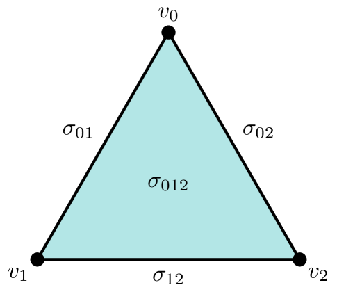
(a) $X$

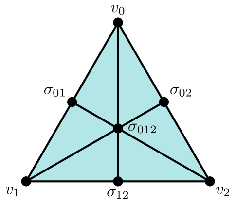
(b) $\mathcal{K}(X)$

Figure 16. We represent the barycentric subdivision of a simplicial complex identifying the vertices in $\mathcal{K}(X)$ with the barycenters of the corresponding simplices.

Definition 4.13.

Given a simplicial complex $X$, its barycentric subdivision, denoted by $\mathcal{K}(X)$, is defined as the simplicial complex whose set of vertices is the set of simplices in $X$ and whose simplices are the sets of simplices $(\sigma_{0},\sigma_{1},\dots,\sigma_{n})$ which are totally ordered by the face relation in $X$, $\sigma_{0}{\trianglelefteqslant}\sigma_{1}{\trianglelefteqslant}\dots\trianglelefteqslant\sigma_{n}$.

An important characteristic of the barycentric subdivision is that it preserves the topological properties of the simplicial complex. In particular, $X$ and $\mathcal{K}(X)$ have isomorphic cohomology spaces: $H^{n}(X;\Bbbk)\simeq H^{n}(\mathcal{K}(X);\Bbbk)$ [50, Theorem 17.2].

Definition 4.14.

Let $X$ be a simplicial complex. The star of a simplex $\sigma\in X$ is the set of simplices that contain $\sigma$ as a face. It is denoted as

$$\text{st}_{X}(\sigma)=\{\tau\in X:\sigma{\trianglelefteqslant}\tau\}$$

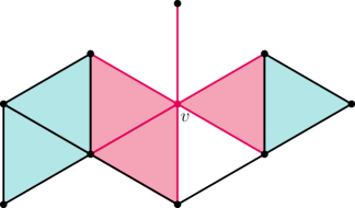
Figure 17. In pink, the star of the vertex $v$.

Definition 4.15.

Let $\mathbf{h}=\{h_{0},h_{1},\dots,h_{m}\}$ be as before. Given a simplicial complex $X$, we define the $\mathbf{h}$-barycentric subdivision of $X$, $\mathcal{K}(X)^{\mathbf{h}}$, as the simplicial complex defined by the simplices $(\sigma_{0},\sigma_{1},\dots,\sigma_{n})$ in its barycentric subdivision such that $\dim\sigma_{i}\in\mathbf{h}$ for all $0\leq i\leq n$. That is, $\mathcal{K}(X)^{\mathbf{h}}$ is the simplicial complex obtained by removing from $\mathcal{K}(X)$ the stars of the vertices of $\mathcal{K}(X)$ associated with the simplices in $X$ whose dimension is not in $\mathbf{h}$,

$$\mathcal{K}(X)^{\mathbf{h}}=\mathcal{K}(X)\smallsetminus\bigcup_{\dim\sigma\notin\mathbf{h}}\text{st}_{\mathcal{K}(X)}(\sigma)$$

Proposition 4.16.

The sheaf cohomology of the constant sheaf $\Bbbk$ over the $\mathbf{h}$-face poset is isomorphic to the simplicial cohomology with coefficients in $\Bbbk$ of the $\mathbf{h}$-barycentric subdivision,

$$H^{n}(P_{X}^{\mathbf{h}};\Bbbk)\simeq H^{n}(\mathcal{K}(X)^{\mathbf{h}};\Bbbk)$$

As a consequence,

$$\beta^{n,\mathbf{h}}(X;\Bbbk)=\dim H^{n}(\mathcal{K}(X)^{\mathbf{h}};\Bbbk)$$

Proof.

It follows from the fact that cochain spaces and coboundary maps induced by the standard resolution associated with the constant sheaf $\Bbbk$ over the finite space $P_{X}^{\mathbf{h}}$ (Equations (6) and (7)) coincide with cochain spaces and coboundary maps associated with simplicial cohomology with coefficients in $\Bbbk$ of the simplicial complex $\mathcal{K}(X)^{\mathbf{h}}$ (Equations (2) and (3)). ∎

Example 4.17.

Let $X$ be the simplicial complex in Figure 6A. Taking $\mathbf{h}=\{0,2\}$, that is, removing the edges from $X$, we obtain the following cohesive Betti numbers

$$\beta^{0,\{0,2\}}(X;\mathbb{Z}_{2})=1\ \ \text{ and }\ \ \beta^{1,\{0,2\}}(X;\mathbb{Z}_{2})=1$$

They correspond with the topological properties of the $\{0,2\}$-barycentric subdivision (Figure 18A): the simplicial complex $\mathcal{K}(X)^{\{0,2\}}$ has a connected component and a hole.

When we instead remove the vertices, $\mathbf{h}=\{1,2\}$, we obtain cohesive Betti numbers

$$\beta^{0,\{1,2\}}(X;\mathbb{Z}_{2})=3\ \ \text{ and }\ \ \beta^{1,\{0,2\}}(X;\mathbb{Z}_{2})=0$$

This corresponds to the three connected components and the absence of holes in $\mathcal{K}(X)^{\{1,2\}}$ (Figure 18B).

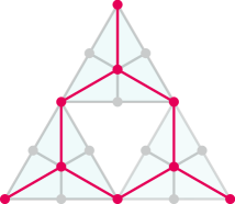
(a) $\mathcal{K}(X)^{\{0,2\}}$

(b) $\mathcal{K}(X)^{\{1,2\}}$

Figure 18. Barycentric subdivision of simplicial complex in Figure 6A and the corresponding subcomplexes $\mathcal{K}(X)^{\{0,2\}}$ and $\mathcal{K}(X)^{\{1,2\}}$ (marked in pink).

5. Resilience: thick and cohesive bipersistence.

This section is devoted to explaining how the resilience of holes and connected components in simplicial networks subject to attacks (involving the removal of simplices across different dimensions) can be analyzed through a specific type of biparameter persistence module, where one parameter reflects the attack cofiltration index, and the other corresponds to the index of a cofiltration based either on coskeleta or on cohesiveness.

5.1. Resilience of thick holes.

Let

$$X^{\bullet}\colon X=X^{0}\supseteq X^{1}\supseteq X^{2}\supseteq\dots\supseteq X^{N}$$ (14)

be a cofiltration of simplicial complexes modelling an arbitrary degenerative process (in which vertices, edges, triangles, etc., may disappear at each step). As illustrated in Section 3.2, a comprehensive study of the thickness of the holes requires a dynamic perspective. In this sense, for each $X^{i}$ we have the cofiltration defined by its coskeletons:

$$X^{i,\bullet}\colon X^{i,0}\supseteq X^{i,1}\supseteq X^{i,2}\supseteq\dots\supseteq X^{i,M}$$

Varying both parameters, $i=1,\dots,N$ and $h=1,\dots,M$, we obtain a biparameter persistence module (Example 2.16):

(15)

The horizontal axis ($i$) reveals how features emerge or disappear as simplices are removed from the initial complex, while the vertical axis ($h$) tracks how features change when restricting to higher-dimensional simplices.

One of the main challenges in multipersistence lies in the absence of a straightforward generalization of the barcode decomposition theorem (Remark 2.21). Consequently, inspired by the framework introduced in [26] and for each h = 1,…,M, we focus our attention on the following diagram:

(16)

which allow us to analyze the subsequent collection of one parameter persistence modules:

• The $n$-th persistence module of the cofiltration modelling the degenerative process, on the bottom horizontal line,

  $$H^{n}(X^{\bullet};\Bbbk):H^{n}(X^{0};\Bbbk)\to H^{n}(X^{1};\Bbbk)\to\cdots\to H^{n}(X^{N};\Bbbk)\to 0$$

• The $n$-th persistence module of the $h$-coskeleton of the cofiltration, on the top horizontal line,

  $$H^{n}(X^{\bullet,h};\Bbbk):H^{n}(X^{0,h};\Bbbk)\to H^{n}(X^{1,h};\Bbbk)\to\cdots\to H^{n}(X^{N,h};\Bbbk)\to 0$$

• The image persistence module

  $$\operatorname{im}\varphi^{n,\bullet,h}:\operatorname{im}\varphi^{n,0,h}\to\operatorname{im}\varphi^{n,1,h}\to\cdots\to\operatorname{im}\varphi^{n,N,h}\to 0$$

  It registers the persistence of holes enclosed by simplices of dimension at least $h$ within the cofiltration $X^{\bullet}$.

• The kernel persistence module

  $$\ker\varphi^{n,\bullet,h}:\ker\varphi^{n,0,h}\to\ker\varphi^{n,1,h}\to\cdots\to\ker\varphi^{n,N,h}\to 0$$

  It captures the evolution of holes that are enclosed by simplices of dimension less than $h$ as the cofiltration $X^{\bullet}$ progresses.

• The cokernel persistence module

  $$\operatorname{coker}\varphi^{n,\bullet,h}:\operatorname{coker}\varphi^{n,0,h}\to\operatorname{coker}\varphi^{n,1,h}\to\cdots\to\operatorname{coker}\varphi^{n,N,h}\to 0$$

  It encodes the persistence of cohomology classes that emerge when simplices outside the $h$-coskeleton are removed.

Let us illustrate this study with the following examples.

Example 5.1.

In Figure 19A we have a cofiltration of simplicial complexes with $5$ steps. In the first step, $X^{0}$, there is a $1$-dimensional hole that is fully enclosed by triangles ($2$-simplices). Along the cofiltration, some of the triangles surrounding the hole disappear, resulting in a thinning of the hole. However, the persistence barcode of the filtration do not capture any change in the structure of the simplicial complexes (Figure 19C). Examining the cofiltration of $2$-coskeletons (Figure 19B), we observe that the hole disappears at step 4. The persistence barcode of the cofiltration $X^{\bullet,2}$ (Figure 19D) reflects that the hole in $X^{\bullet}$ is no longer enclosed by triangles in $X^{4}$. In this way, although the hole persists throughout the cofiltration, we can see that it is suffering some damage, causing a loss of thickness that could indicate a future disappearance of the hole. It is worth noting that, in this example, the image, kernel, and cokernel persistence modules offer little additional insight beyond what is already captured by the persistence module of the $2$-coskeleton. In Example 5.2 we present a case where such information is less immediately accessible.

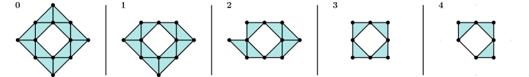
(a) Cofiltration $X^{\bullet}$

(b) Cofiltration $X^{\bullet,2}$

(c) Barcodes of cofiltration $X^{\bullet}$

(d) Barcodes of cofiltration $X^{\bullet,2}$

Figure 19. Cofiltration of simplicial complexes, cofiltration of $2$-coskeletons and their corresponding barcodes

Example 5.2.

Figure 20 shows a cofiltration and the associated persistence barcodes for $h=2$. We focus here on $0$-th cohomology, that is, on the evolution of connected components. In the cofiltration $X^{\bullet}$ there are two connected components: one persists throughout the entire cofiltration, and another is born at step 1 and dies at step 3.

The image barcode indicates that the long-persistent connected component in $X^{\bullet}$ is defined by triangles whereas the shorter-lived component is defined by lower dimensional simplices at step $2$, which is when its corresponding bar is born in the kernel persistence module. The bar in $\ker\varphi^{0,\bullet,2}$ reflects the thinning of the connected component, anticipating its disappearance. Finally, the bar in the cokernel persistence module reflects the connected component that emerges at step 0 when passing to the $2$-coskeleta, which become a connected component of $X^{\bullet}$ at step 1.

(a) Cofiltration $X^{\bullet}$

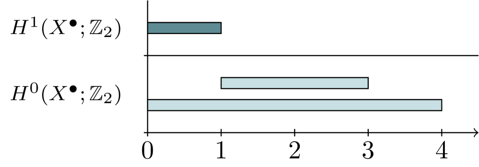
(b) Barcodes of the cofiltration $X^{\bullet}$

(c) Barcode of the cofiltration of $2$-coskeletons

(d) Barcode of the image persistence module

(e) Barcode of the kernel persistence module

(f) Barcode of the cokernel persistence module

Figure 20. Cofiltration of simplicial complexes and persistence barcodes arising from the $2$-coskeletons

5.2. Resilience of cohesive holes.

Example 5.1 illustrates the utility of thick Betti numbers in analyzing the degenerative dynamics of a simplicial network. However, Figure 19 indicates that such an approach is not sufficient to fully characterize the network’s degradation, a gap we address through cohesive Betti numbers in this section.

Given the cofiltration in equation (14):

$$X^{\bullet}\colon X=X^{0}\supseteq X^{1}\supseteq X^{2}\supseteq\dots\supseteq X^{N}\,,$$

for each $\mathbf{h}=\{h_{0},h_{1},\dots,h_{m}\}$, the $\mathbf{h}$-face posets of simplicial complexes $X^{\bullet}$ form a cofiltration of finite topological spaces:

$$P^{\mathbf{h}}_{X^{\bullet}}\colon P_{X^{0}}^{\mathbf{h}}\supseteq P_{X^{1}}^{\mathbf{h}}\supseteq P_{X^{2}}^{\mathbf{h}}\supseteq\dots\supseteq P_{X^{N}}^{\mathbf{h}}$$

Cofiltration $P^{\mathbf{h}}_{X^{\bullet}}$ and the corresponding linear maps $\varphi^{n,h}_{\bullet}$ from equation (13) induce a commutative diagram:

(17)

Similar to the previous section, from diagram (17) we get the following collection of persistence modules:

• The $n$-th persistence module of the cofiltration, on the bottom horizontal line,

  $$H^{n}(X^{\bullet};\Bbbk)\,\colon\ H^{n}(X^{0};\Bbbk)\to H^{n}(X^{1};\Bbbk)\to\dots\to H^{n}(X^{N};\Bbbk)\to 0$$

• The $n$-th persistence module of the cofiltration of $\mathbf{h}$-face posets, $P_{X^{\bullet}}^{\mathbf{h}}$, on the top horizontal line,

  $$H^{n}(P_{X^{\bullet}}^{\mathbf{h}};\Bbbk)\,\colon\ H^{n}(P_{X^{0}}^{\mathbf{h}};\Bbbk)\to H^{n}(P_{X^{1}}^{\mathbf{h}};\Bbbk)\to\dots\to H^{n}(P_{X^{N}}^{\mathbf{h}};\Bbbk)\to 0$$

• The image persistence module

  $$\operatorname{im}\varphi_{\bullet}^{n,\mathbf{h}}\,\colon\ \operatorname{im}\varphi_{0}^{n,\mathbf{h}}\to\operatorname{im}\varphi_{1}^{n,\mathbf{h}}\to\dots\to\operatorname{im}\varphi_{N}^{n,\mathbf{h}}\to 0$$

  It tracks the evolution of the holes in the cofiltration $X^{\bullet}$ defined by simplices whose dimension is in $\mathbf{h}$.

• The kernel persistence module

  $$\ker\varphi_{\bullet}^{n,\mathbf{h}}\,\colon\ \ker\varphi_{0}^{n,\mathbf{h}}\to\ker\varphi_{1}^{n,\mathbf{h}}\to\dots\to\ker\varphi_{N}^{n,\mathbf{h}}\to 0$$

  It records the evolution throughout the cofiltation $X^{\bullet}$ of the holes that disappear when removing simplices whose dimension is not in $\mathbf{h}$ (the less cohesive ones).

• The cokernel persistence module

  $$\operatorname{coker}\varphi_{\bullet}^{n,\mathbf{h}}\,\colon\ \operatorname{coker}\varphi_{0}^{n,\mathbf{h}}\to\operatorname{coker}\varphi_{1}^{n,\mathbf{h}}\to\dots\to\operatorname{coker}\varphi_{N}^{n,\mathbf{h}}\to 0$$

  It contains the dynamics of the holes that are created by the elimination of simplices.

Remark 5.3.

In practice, the study of the persistence modules defined by diagram (17) is equivalent (Section 4.3) to the study of the corresponding persistence modules associated with the following diagram

(18)

Here, the horizontal linear maps are induced respectively by the cofiltrations $\mathcal{K}(X^{\bullet})$ and $\mathcal{K}(X^{\bullet})^{\mathbf{h}}$ and the vertical linear maps $\varphi^{n,\mathbf{h}}_{\bullet}$ are defined by the inclusions $\mathcal{K}(X^{\bullet})^{\mathbf{h}}\subseteq\mathcal{K}(X^{\bullet})$. This perspective helps to visualize the information encoded by diagram (17), as we will see in Example 5.4.

Example 5.4.

Let us continue with the analysis of the cofiltration in Example 5.1 as previously pointed out. We adopt the viewpoint of the barycentric subdivision (see Section 4.3) and reinterpret the degeneration cofiltration presented in Example 5.1 accordingly (see Figure 21A).

Figure 21D shows the persistence barcodes associated with the $\{0,2\}$-face poset cofiltration. We observe that many bars appear in $H^{1}(P_{X^{\bullet}}^{\{0,2\}};\mathbb{Z}_{2})$. The $\{0,2\}$-barycentric subdivision cofiltration (Figure 21B) illustrates the persistence of such bars. Moreover, comparing with $\mathcal{K}(X^{\bullet})$ (Figure 21A), we can see that most of the bars in $H^{1}(P_{X^{\bullet}}^{\{0,2\}};\mathbb{Z}_{2})$ correspond to holes that are created by edge removal. From an algebraic point of view, the persistence of such holes is given by cokernel persistence barcode $\operatorname{coker}\varphi^{1,\{0,2\}}_{\bullet}$ (Figure 21H). To focus on the persistence of the hole in $X^{\bullet}$ when edges are removed, we study the image persistence module $\operatorname{im}\varphi^{1,\{0,2\}}_{\bullet}$ (Figure 21F). As its barcode shows, in this example it captures the same information as the $2$-coskeleton cofiltration barcode (Figure 19D), reflecting that the hole in $X^{\bullet}$ is no longer fully surrounded by triangles in stage 4.

On the other hand, the persistence barcode $\operatorname{im}\varphi^{1,\{1,2\}}_{\bullet}$ (Figure 21F) consists of the interval $[0,1)$, meaning that the hole in $X^{\bullet}$ is only enclosed by a closed $(1,2)$-walk in $X^{0}$. Thus, the study of the cohesion of the network detects that the deterioration affects the hole from the very first stage. Further information is provided by the intervals in $\operatorname{coker}\varphi^{0,\{1,2\}}_{\bullet}$ (Figure 21I). When we remove the vertices, two $(1,2)$-connected components are born in step $2$ and one more is born in step $3$, although neither connectivity nor $(0,2)$-connectivity are affected along the original cofiltration (Figures 19C and 21D). This points to an increase of critical vertices in the network.

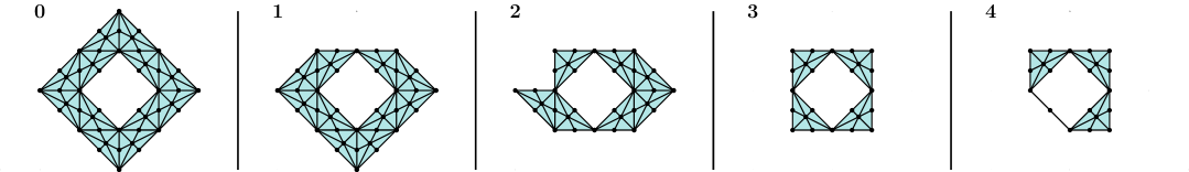
(a) Cofiltration $\mathcal{K}(X^{\bullet})$

(b) Cofiltration $\mathcal{K}(X^{\bullet})^{\{0,2\}}$

(c) Cofiltration $\mathcal{K}(X^{\bullet})^{\{1,2\}}$

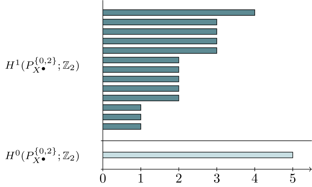
(d) Barcodes of the $\{0,2\}$-face posets cofiltration

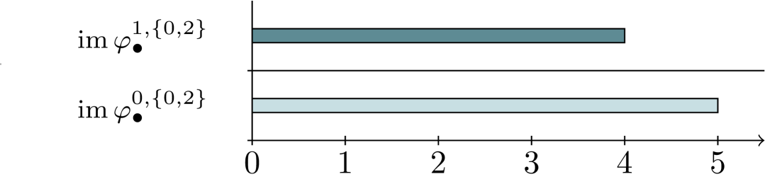
(e) Barcodes of the $\{0,2\}$-image persistence modules

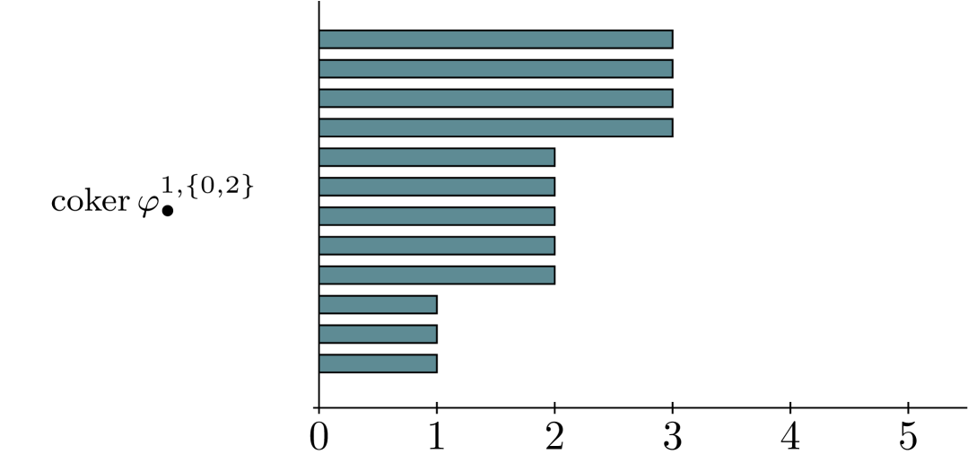
(f) Barcode of the $\{0,2\}$-cokernel persistence modules

(g) Barcodes of the $\{1,2\}$-face posets cofiltration

(h) Barcodes of the $\{1,2\}$-image persistence modules

(i) Barcode of the $\{1,2\}$-cokernel persistence modules

Figure 21. Barycentric subdivision cofiltrations and persistence barcodes

Remark 5.5.

Notice that from diagrams (16) and (18) emerges an additional $1$-parameter persistence module, defined by relative simplicial cohomology, completing the so-called 6-pack [28], which was not examined in this work.

Remark 5.6.

Cohen-Steiner et al. [26] developed algorithms to compute the barcodes of the image, kernel and cokernel persistence modules arising from an inclusion of simplicial filtrations. However, to the best of our knowledge, few public implementations are available. One such implementation is provided by Bauer and Schmahl [11], who integrated an algorithm for image persistence into the Ripser framework [10], enabling efficient barcode computation for an inclusion of Vietoris-Rips filtrations.

6. Conclusion

In this work, we have proposed a novel approach to studying the robustness of simplicial networks through the lens of Topological Data Analysis. Motivated by the limitations of classical Betti numbers in capturing the structural intricacies of higher-order interactions, we introduced two new families of invariants: the thick Betti numbers, which quantify the dimensional thickness of homology cycles, and the cohesive Betti numbers, which assess the strength of higher-order adjacencies among the simplices forming such cycles. As shown in Figure 22, despite sharing the same homotopy type, the three simplicial complexes differ in structural aspects that the Betti numbers proposed here successfully detect.

$\begin{gathered}\beta^{1}(X;\mathbb{Z}_{2})=1\\[4.30554pt] \beta^{1}_{0,2}(X;\mathbb{Z}_{2})=1\\[4.30554pt] \beta^{1,\{0,2\}}_{\operatorname{im}}(X;\mathbb{Z}_{2})=1\\[4.30554pt] \beta^{1,\{1,2\}}_{\operatorname{im}}(X;\mathbb{Z}_{2})=1\end{gathered}$

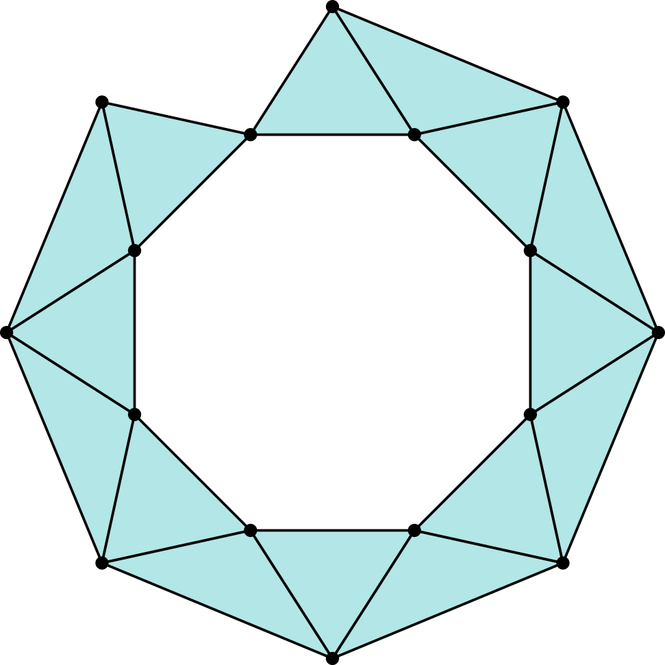
$\begin{gathered}\beta^{1}(Y;\mathbb{Z}_{2})=1\\[4.30554pt] \beta^{1}_{0,2}(Y;\mathbb{Z}_{2})=1\\[4.30554pt] \beta^{1,\{0,2\}}_{\operatorname{im}}(Y;\mathbb{Z}_{2})=1\\[4.30554pt] \beta^{1,\{1,2\}}_{\operatorname{im}}(Y;\mathbb{Z}_{2})=0\end{gathered}$

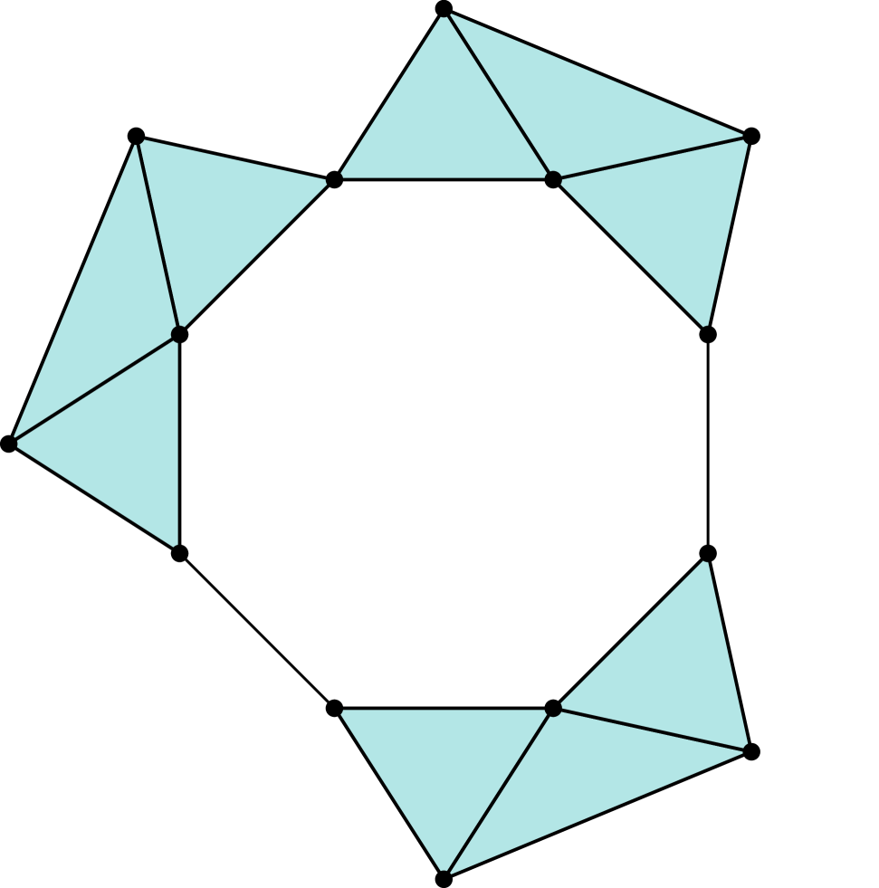
$\begin{gathered}\beta^{1}(Z;\mathbb{Z}_{2})=1\\[4.30554pt] \beta^{1}_{0,2}(Z;\mathbb{Z}_{2})=0\\[4.30554pt] \beta^{1,\{0,2\}}_{\operatorname{im}}(Z;\mathbb{Z}_{2})=0\\[4.30554pt] \beta^{1,\{1,2\}}_{\operatorname{im}}(Z;\mathbb{Z}_{2})=0\end{gathered}$

Figure 22. Simplicial complexes that are homotopy equivalent yet differ in subtle structural features, which are effectively captured by the refined Betti numbers introduced in this work.

By modeling different simplicial degradation processes using cofiltrations–based on coskeleta and dimension-specific removals–we demonstrated how these invariants offer a finer topological characterization of robustness beyond what is measurable by classical persistence. Furthermore, we extended this framework through biparameter persistence modules, which allow us to jointly track both the evolution of structural damage (attacks) and the underlying topological refinement related to cycle thickness or cohesiveness. This dual-parameter perspective opens new directions for theoretical studies of topological resilience in higher order complex systems.

While the proposed invariants provide meaningful insights into the internal structure and stability of topological features, several limitations remain. First, the cohesive Betti numbers require a sheaf-theoretic cohomological formalism, which may pose conceptual and computational challenges for practical applications. Second, the computational cost associated with barycentric subdivision presents a significant challenge when working with very large or high-dimensional complexes, potentially limiting scalability. Additionally, the current lack of publicly available software for computing kernel and cokernel persistence modules restricts broader adoption and impedes the full reproducibility of our proposed pipeline.

Looking forward, we envision several applications of this work. In particular, these methods could be useful for early detection of degenerative diseases, such as neurodegeneration or cardiac dysfunction, where the progressive removal of simplices models the degradation of biological connectivity. Other possible areas include cancer propagation, contagion dynamics, and topological deep learning, where understanding the robustness of higher-order interactions is crucial. While such applications are beyond the scope of the current paper, they will be explored in future work.

References

- [1] R. Albert and A.-L. Barabási, Statistical mechanics of complex networks, Rev. Mod. Phys., 74 (2002), pp. 47–97.
- [2] R. Atkin, From cohomology in physics to q-connectivity in social science, International Journal of Man-Machine Studies, 4 (1972), pp. 139–167.
- [3] A.-L. Barabasi and R. Albert, Emergence of scaling in random networks, Science, 286 (1999), pp. 509–512.
- [4] A.-L. Barabási and M. Pósfai, Network science, Cambridge University Press, Cambridge, 2016.
- [5] J. A. Barmak, Algebraic topology of finite topological spaces and applications, vol. 2032 of Lecture Notes in Mathematics, Springer, Heidelberg, 2011.
- [6] A. Barrat, G. Ferraz de Arruda, I. Iacopini, and Y. Moreno, Social contagion on higher-order structures, in Higher-Order Systems, Springer, 2021, pp. 163–184.
- [7] M. Barsbey, R. Ballester, A. Demir, C. Casacuberta, P. Hernández-García, D. Pujol-Perich, S. Yurtseven, S. Escalera, C. Battiloro, M. Hajij, and T. Birdal, Higher-order molecular learning: The cellular transformer, in ICLR 2025 Workshop on Generative and Experimental Perspectives for Biomolecular Design, 2025.
- [8] C. Battiloro, E. Karaismailoǧlu, M. Tec, G. Dasoulas, M. Audirac, and F. Dominici, E(n) equivariant topological neural networks, in International Conference on Learning Representations (ICLR), 2025.
- [9] F. Battiston, G. Cencetti, I. Iacopini, V. Latora, M. Lucas, A. Patania, J.-G. Young, and G. Petri, Networks beyond pairwise interactions: structure and dynamics, Phys. Rep., 874 (2020), pp. 1–92.
- [10] U. Bauer, Ripser: efficient computation of Vietoris-Rips persistence barcodes, J. Appl. Comput. Topol., 5 (2021), pp. 391–423.
- [11] U. Bauer and M. Schmahl, Efficient Computation of Image Persistence, in 39th International Symposium on Computational Geometry (SoCG 2023), E. W. Chambers and J. Gudmundsson, eds., vol. 258 of Leibniz International Proceedings in Informatics (LIPIcs), Dagstuhl, Germany, 2023, Schloss Dagstuhl – Leibniz-Zentrum für Informatik, pp. 14:1–14:14.
- [12] G. Bianconi and R. M. Ziff, Topological percolation on hyperbolic simplicial complexes, Phys. Rev. E, 98 (2018), p. 052308.
- [13] C. Bick, E. Gross, H. A. Harrington, and M. T. Schaub, What are higher-order networks?, SIAM Review, 65 (2023), pp. 686–731.
- [14] S. Boccaletti, V. Latora, Y. Moreno, M. Chavez, and D.-U. Hwang, Complex networks: Structure and dynamics, Physics Reports, 424 (2006), pp. 175–308.
- [15] M. B. Botnan and W. Crawley-Boevey, Decomposition of persistence modules, Proc. Amer. Math. Soc., 148 (2020), pp. 4581–4596.
- [16] M. B. Botnan and M. Lesnick, An introduction to multiparameter persistence, in Representations of algebras and related structures, EMS Ser. Congr. Rep., EMS Press, Berlin, [2023] ©2023, pp. 77–150.
- [17] G. E. Bredon, Sheaf theory, vol. 170 of Graduate Texts in Mathematics, Springer-Verlag, New York, second ed., 1997.
- [18] Z. Cang and G.-W. Wei, Topologynet: Topology based deep convolutional and multi-task neural networks for biomolecular property predictions, PLOS Computational Biology, 13 (2017), pp. 1–27.
- [19] G. Carlsson, Topology and data, AMS Bulletin, 46 (2009), pp. 255–308.
- [20] G. Carlsson, Persistent homology and applied homotopy theory, in Handbook of homotopy theory, CRC Press/Chapman Hall Handb. Math. Ser., CRC Press, Boca Raton, FL, [2020] ©2020, pp. 297–330.
- [21] G. Carlsson, A. Zomorodian, A. Collins, and L. Guibas, Persistence barcodes for shapes, in Proceedings of the 2004 Eurographics/ACM SIGGRAPH Symposium on Geometry Processing, SGP ’04, New York, NY, USA, 2004, Association for Computing Machinery, pp. 124–135.
- [22] V. Carmona Sánchez, C. Maestro Pérez, F. Sancho de Salas, and J. Torres Sancho, Homology and cohomology of finite spaces, Journal of Pure and Applied Algebra, 224 (2020), p. 106200.
- [23] F. Chazal and B. Michel, An introduction to topological data analysis: Fundamental and practical aspects for data scientists, Frontiers in Artificial Intelligence, Volume 4 - 2021 (2021).
- [24] Q. Chen, Y. Zhao, C. Li, and X. Li, Robustness of higher-order networks with synergistic protection, New Journal of Physics, 25 (2023), p. 113045.
- [25] S. Chowdhary, A. Kumar, G. Cencetti, I. Iacopini, and F. Battiston, Simplicial contagion in temporal higher-order networks, Journal of Physics: Complexity, 2 (2021), p. 035019.
- [26] D. Cohen-Steiner, H. Edelsbrunner, J. Harer, and D. Morozov, Persistent homology for kernels, images, and cokernels, in Proceedings of the Twentieth Annual ACM-SIAM Symposium on Discrete Algorithms, SODA ’09, USA, 2009, Society for Industrial and Applied Mathematics, pp. 1011–1020.
- [27] C. Curto, What can topology tell us about the neural code?, Bull. Amer. Math. Soc. (N.S.), 54 (2017), pp. 63–78.
- [28] S. C. di Montesano, O. Draganov, H. Edelsbrunner, and M. Saghafian, Chromatic alpha complexes, 2024.
- [29] P. Doreian, On the evolution of group and network structure, Social Networks, 2 (1979), pp. 235–252.
- [30] H. Edelsbrunner, D. Letscher, and A. Zomorodian, Topological persistence and simplification, Discrete Comput. Geom., 28 (2002), pp. 511–533. Discrete and computational geometry and graph drawing (Columbia, SC, 2001).
- [31] L. C. Freeman, Q-analysis and the structure of friendship networks, International Journal of Man-Machine Studies, 12 (1980), pp. 367–378.
- [32] J. Gallier and J. Quaintance, Homology, Cohomology, and Sheaf Cohomology for Algebraic Topology, Algebraic Geometry, and Differential Geometry, World Scientific, 2022.
- [33] E. Gawrilow and M. Joswig, polymake: a Framework for Analyzing Convex Polytopes, Birkhäuser Basel, Basel, 2000, pp. 43–73.
- [34] R. Ghrist, Barcodes: The persistent topology of data, Bull. Amer. Math. Soc., 45 (2008), pp. 61–75.
- [35] R. Ghrist, Homological algebra and data, in The mathematics of data, vol. 25 of IAS/Park City Math. Ser., Amer. Math. Soc., Providence, RI, 2018, pp. 273–325.
- [36] C. Giusti, R. Ghrist, and D. S. Bassett, Two’s company, three (or more) is a simplex, J. Comput. Neurosci., 41 (2016), pp. 1–14.
- [37] C. Giusti, E. Pastalkova, C. Curto, and V. Itskov, Clique topology reveals intrinsic geometric structure in neural correlations, Proc. Natl. Acad. Sci. USA, 112 (2015), pp. 13455–13460.
- [38] D. R. Grayson and M. E. Stillman, Macaulay2, a software system for research in algebraic geometry. Available at http://www2.macaulay2.com.
- [39] M. Hajij, G. Zamzmi, T. Papamarkou, V. Maroulas, and X. Cai, Simplicial complex representation learning, 2021.
- [40] M. Hajij, G. Zamzmi, T. Papamarkou, N. Miolane, A. Guzmán-Sáenz, K. N. Ramamurthy, T. Birdal, T. K. Dey, S. Mukherjee, S. N. Samaga, N. Livesay, R. Walters, P. Rosen, and M. T. Schaub, Topological deep learning: Going beyond graph data, 2023.
- [41] A. Hatcher, Algebraic topology, Cambridge University Press, Cambridge, 2002.
- [42] D. Hernández Serrano, J. Hernández-Serrano, and D. Sánchez Gómez, Simplicial degree in complex networks. Applications of topological data analysis to network science, Chaos Solitons Fractals, 137 (2020), pp. 109839, 21.
- [43] D. Hernández Serrano and D. Sánchez Gómez, Centrality measures in simplicial complexes: applications of topological data analysis to network science, Appl. Math. Comput., 382 (2020), pp. 125331, 21.
- [44] I. Iacopini, G. Petri, A. Barrat, and V. Latora, Simplicial models of social contagion, Nature Communications, 10 (2019), p. 2485.
- [45] M. Lesnick and M. Wright, Interactive visualization of 2-d persistence modules, 2015.
- [46] Z. Lin, L. Han, M. Feng, Y. Liu, and M. Tang, Higher-order non-markovian social contagions in simplicial complexes, Communications Physics, 7 (2024).
- [47] S. Maletić and M. Rajkovic, Combinatorial laplacian and entropy of simplicial complexes associated with complex networks, The European Physical Journal Special Topics, 212 (2012), pp. 77–97.
- [48] J. T. Matamalas, S. Gómez, and A. Arenas, Abrupt phase transition of epidemic spreading in simplicial complexes, Phys. Rev. Res., 2 (2020), p. 012049.
- [49] M. C. McCord, Singular homology groups and homotopy groups of finite topological spaces, Duke Mathematical Journal, 33 (1966), pp. 465 – 474.
- [50] J. R. Munkres, Elements of algebraic topology, Addison-Wesley Publishing Company, Menlo Park, CA, 1984.
- [51] D. Nguyen Duc, Z. Cang, K. Wu, M. Wang, Y. Cao, and G.-W. Wei, Mathematical deep learning for pose and binding affinity prediction and ranking in d3r grand challenges, Journal of Computer-Aided Molecular Design, 33 (2019), pp. 1–12.
- [52] D. Nguyen Duc, K. Gao, M. Wang, and G.-W. Wei, Mathdl: mathematical deep learning for d3r grand challenge 4, Journal of Computer-Aided Molecular Design, 34 (2020).
- [53] N. Otter, M. A. Porter, U. Tillmann, P. Grindrod, and H. A. Harrington, A roadmap for the computation of persistent homology, EPJ Data Science, 6 (2017).
- [54] M. Papillon, G. Bernárdez, C. Battiloro, and N. Miolane, Topotune: A framework for generalized combinatorial complex neural networks, 2024.
- [55] M. W. Reimann, M. Nolte, M. Scolamiero, K. Turner, R. Perin, G. Chindemi, P. DÅ’otko, R. Levi, K. Hess, and H. Markram, Cliques of neurons bound into cavities provide a missing link between structure and function, Frontiers in Computational Neuroscience, 11 (2017).
- [56] F. Sancho de Salas, Finite spaces and schemes, J. Geom. Phys., 122 (2017), pp. 3–27.
- [57] D. H. Serrano, J. Villarroel, J. Hernández-Serrano, and A. Tocino, Stochastic simplicial contagion model, Chaos, Solitons & Fractals, 167 (2023), p. 113008.
- [58] A. E. Sizemore, C. Giusti, A. Kahn, J. M. Vettel, R. F. Betzel, and D. S. Bassett, Cliques and cavities in the human connectome, J. Comput. Neurosci., 44 (2018), pp. 115–145.
- [59] A. E. Sizemore, J. E. Phillips-Cremins, R. Ghrist, and D. S. Bassett, The importance of the whole: Topological data analysis for the network neuroscientist, Network Neuroscience, 3 (2019), pp. 656–673.
- [60] N. Swenson, A. S. Krishnapriyan, A. Buluc, D. Morozov, and K. Yelick, Persgnn: Applying topological data analysis and geometric deep learning to structure-based protein function prediction, 2020.
- [61] The RIVET Developers, Rivet. https://github.com/rivetTDA/rivet/, 2020.
- [62] The Sage Developers, SageMath, the Sage Mathematics Software System, 2022. DOI 10.5281/zenodo.6259615.
- [63] A. Tocino, D. Hernández Serrano, J. Hernández-Serrano, and J. Villarroel, A stochastic simplicial sis model for complex networks, Communications in Nonlinear Science and Numerical Simulation, 120 (2023), p. 107161.
- [64] K. Wu and G.-W. Wei, Quantitative toxicity prediction using topology based multitask deep neural networks, Journal of Chemical Information and Modeling, 58 (2018), pp. 520–531. PMID: 29314829.
- [65] A. Zomorodian and G. Carlsson, Computing persistent homology, Discrete Comput. Geom., 33 (2005), pp. 249–274.