Counterfactual Strategies for Markov Decision Processes

Abstract

Counterfactuals are widely used in AI to explain how minimal changes to a model’s input can lead to a different output. However, established methods for computing counterfactuals typically focus on one-step decision-making, and are not directly applicable to sequential decision-making tasks. This paper fills this gap by introducing counterfactual strategies for Markov Decision Processes (MDPs). During MDP execution, a strategy decides which of the enabled actions (with known probabilistic effects) to execute next. Given an initial strategy that reaches an undesired outcome with a probability above some limit, we identify minimal changes to the initial strategy to reduce that probability below the limit. We encode such counterfactual strategies as solutions to non-linear optimization problems, and further extend our encoding to synthesize diverse counterfactual strategies. We evaluate our approach on four real-world datasets and demonstrate its practical viability in sophisticated sequential decision-making tasks.

1 Introduction

Consider an application procedure in which clients who want to obtain a loan, interact with a bank to establish their eligibility. Although established prediction methods Leo et al. (2019); Teinemaa et al. (2019) can be used to filter for eligible clients, the overall application procedure is far from automated. In practice, to receive a loan from the bank, a client must follow a complicated application procedure, involving, e.g., multiple consultations with loan advisors, providing various documents and filling out complex forms. Eligible but impatient clients are prone to abandoning the application procedure before they receive their loan, causing losses for both parties: the client spent time without reaching their goal and the bank invested resources without return. Markov Decision Processes (MDPs) Baier and Katoen (2008) can be used to model such procedures and improve their transparency; however, methods are currently lacking to address questions about recourse and process improvement; e.g., what would enable an ineligible client to obtain a loan? and how can we simplify the application procedure for eligible clients?

Counterfactual explanations can help answer such questions by showing how minimal changes in user applications would lead to a desired change of the output, e.g., to make the client eligible for the previously refused loan. However, most available methods for computing counterfactuals target one-step prediction tasks Guidotti (2024), and are not applicable to sequential decision making settings, where the output of a process is determined by a sequence of steps.

Contributions. To fill this gap, we propose a method to compute counterfactual explanations for sequential decision making processes modeled by an MDP. In each state of these non-deterministic discrete-time models, a finite number of actions with a known probabilistic effect are enabled. During execution, strategies decide which enabled action to execute next. Given an initial strategy that visits some undesired states with a probability above some limit, we propose to compute explanations in terms of counterfactual strategies that reduce the reachability probability below this limit, while staying as close to the initial strategy as possible. To formalize these requirements, we introduce a distance measure $d$ on strategies and encode counterfactual strategy synthesis as nonlinear optimization problems. By enforcing that only user-controllable actions can be selected in the MDP, we ensure that the resulting counterfactual strategies are indeed actionable. Furthermore, we extend our encoding to compute not only a single solution but a collection of counterfactual strategies, which are optimized for diversity, as several studies emphasize that providing different counterfactuals is key for user understanding Russell (2019); Mothilal et al. (2020); Bove et al. (2023). The method is evaluated on four real-world datasets. The evaluation shows that the method is computationally feasible, and can synthesize counterfactual strategies for sophisticated sequential decision making tasks, modeled as MDPs with thousands of states and ten thousands of transitions.

In summary, our main contributions are (1) to introduce counterfactual strategies for MDPs as post-hoc explanations for sequential decision making, (2) to encode a counterfactual strategy synthesis problem for MDPs as a nonlinear optimization problem, (3) to synthesize diverse counterfactual strategies, and (4) to experimentally evaluate the feasibility and performance of our counterfactual strategy synthesis method.

Outline.

After recalling some background on MDPs, nonlinear optimization and counterfactuals in Section 2, we formalize counterfactual strategies for MDPs in Section 3, and present our encoding of the MDP counterfactual synthesis problem as a non-linear optimization problem in Section 4. We evaluate our approach in Section 5, discuss related work in Section 6, and conclude the paper in Section 7.

2 Preliminaries

A (discrete probability) distribution is a function $\mu\colon X\rightarrow[0,1]$ with a discrete domain $X$ such that $\sum_{x\in X}\mu(x)=1$. We write $\textit{Distr}(X)$ for the set of distributions with domain $X$. Given two distributions $\mu_{1}$ and $\mu_{2}$ with domain $X$, their total variation distance is $\Delta(\mu_{1},\mu_{2})=\frac{1}{2}\sum_{x\in X}|\mu_{1}(x)-\mu_{2}(x)|$ (Levin and Peres, 2017, Prop. 4.2), where $|\cdot|$ stays for the absolute value.

For $n\in\mathbb{N}$, $v\in\mathbb{R}^{n}$ and $i=1,\ldots,n$, we denote the $i$th element of $v$ as $v_{i}$, and use the standard norms $\|v\|_{0}=|\{v_{i}\mid v_{i}\neq 0\}|$, $\|v\|_{1}=\sum_{i}|v_{i}|$, and $\|v\|_{\infty}=\max_{i}|v_{i}|$.

2.1 Markov Decision Processes

A Markov decision process (MDP) $\mathcal{M}$ is a tuple $\langle S,A,s_{0},\delta\rangle$, where $S$ is a finite set of states, $A$ is a finite set of actions, $s_{0}\in S$, and $\delta\colon S\times A\rightharpoonup\textit{Distr}(S)$ is a partial function. For each state $s\in S$, let $A(s)$ be the set of all actions $a\in A$ for which $\delta(s,a)$ is defined; we require $A(s)\not=\emptyset$ and say that the actions in $A(s)$ are enabled in $s$. By $\delta(s,a,s^{\prime})$ we denote $\delta(s,a)(s^{\prime})$ if $\delta(s,a)$ is defined and $0$ otherwise.

A (finite or infinite) path $\tau$ of $\mathcal{M}$ is a non-empty sequence of alternating states and actions $s_{0}a_{0}s_{1}\dots$ such that $\delta(s_{j},a_{j},s_{j+1})>0$ for all $j\geq 0$. The cylinder set $\textit{Cyl}(\hat{\tau})$ of a finite path $\hat{\tau}$ is the set of all infinite paths with $\hat{\tau}$ as a prefix. Let $\Omega_{\mathcal{M}}(s)$ and and $\Omega^{\textit{fin}}_{\mathcal{M}}(s)$ be the set of all infinite respectively finite paths of $\mathcal{M}$ starting in the state $s\in S$.

A state $t\in S$ can be reached from state $s\in S$ if there exists a finite path from $s$ to $t$. We use $\textit{Reach}(t)$ to denote the set of all states from which $t$ can be reached.

A (memoryless) strategy is a function $\sigma\colon S\to\textit{Distr}(A)$ that maps states to distributions over actions with $\sigma(s)(a)=0$ for all $s\in S$ and $a\in A{\setminus}A(s)$. We denote the set of strategies for $\mathcal{M}$ by $\Sigma_{\mathcal{M}}$; we omit the index if it is clear from the context. Given two strategies $\sigma,\sigma^{\prime}\in\Sigma$, we overload notation and define their distance vector as $\Delta(\sigma,\sigma^{\prime})=(\Delta(\sigma(s),\sigma^{\prime}(s)))_{s\in S}$ (entries in fixed but arbitrary order).

Applying a strategy $\sigma$ to an MDP $\mathcal{M}$ induces a deterministic model. Thus we omit the actions and define the discrete-time Markov chain (DTMC) induced by $\sigma$ on $\mathcal{M}$ as the tuple $\mathcal{M}^{\sigma}=\langle S,s_{0},\delta^{\sigma}\rangle$ with $S$ and $s_{0}$ as before and $\delta^{\sigma}\colon S\times S\to[0,1]$ with $\delta^{\sigma}(s,s^{\prime})=\sum_{a\in A}\sigma(s)(a)\cdot\delta(s,a,s^{\prime})$ for all $s,s^{\prime}\in S$.

We associate with $\mathcal{D}{=}\mathcal{M}^{\sigma}$ the probability space $(\Omega_{\mathcal{D}}(s_{0}),\allowbreak\{\bigcup_{\hat{\tau}\in R}\textit{Cyl}(\hat{\tau})\mid R~\subseteq~\Omega^{\textit{fin}}_{\mathcal{D}}(s_{0})\},\allowbreak\textit{Pr}_{\mathcal{D}}(s_{0}))$ where the probability of the cylinder set of a finite path $\hat{\tau}=s_{0}\ldots s_{n}$ is $\textit{Pr}_{\mathcal{D}}(s_{0})(\textit{Cyl}(\hat{\tau}))=\prod_{i=1}^{n}\delta(s_{i-1},s_{i})$. By $\textit{Pr}_{\mathcal{D}}(s_{0},t)$ we denote the probability of reaching state $t\in S$ from $s_{0}$ in $\mathcal{D}$.

(a) MDP model. The only service provider action Provider appears deterministically, thus the user has full strategy control.

	Apply	Consult	Quit	Submit
$s_{0}$	1	0	0	0
Error	0	0.2	0.8	0
Consultation	0	0	1	0
Rework	0	0	0.7	0.3

(b) Probability values $\sigma(s)(a)$ of the impatient client strategy $\sigma$.

	Apply	Consult	Quit	Submit
$s_{0}$	1	0	0	0
Error	0	0.2	0.8	0
Consultation	0	0	1	0
Rework	0	0	0.14	0.86

(c) Counterfactual strategy $\sigma^{*}$ for the impatient client.

Figure 1: Running example of a loan application procedure.

Example 1.

Figure 1(a) shows an MDP model $\mathcal{M}$ of a loan application procedure. Starting in $s_{0}$, the client either directly fills out an application or requests a consultation to increase the probability of direct acceptance. However, when independently filling out the application, there is a $5\%$ chance to make a mistake in the application, which requires a consultation to fix. If the application is not accepted directly, it can be reworked before it is evaluated. The client may decide to quit the application procedure after making a mistake in the form, after the consultation, or if the application is not directly accepted. The behavior of the service provider is captured by several occurrences of the Provider action.

The client’s goal is to receive a loan, i.e. reach the Rejected state with a probability of at most $20\%$. For an impatient client who directly fills out the application using strategy $\sigma\in\Sigma_{\mathcal{M}}$ in Fig. 1(b), the probability of reaching Rejected is $Pr_{\mathcal{M}^{\sigma}}(s_{0},\textit{Rejected})=0.411$.

2.2 Non-linear Optimization

Mixed Integer Quadratically Constrained Quadratic Problems (MIQCQPs) Billionnet et al. (2016) are a class of non-linear optimization problems, where the objective function and the constraints are at most quadratic in variables with real and integer domains. Formally, an MIQCQP has the form

$$\begin{array}[]{lll}\min&f_{0}(x)\\ \text{subject to }&f_{i}(x)\leq b_{i}&\textit{for\ \ }i=1,\dots,m,\\ &0\leq x_{j}\leq u_{j}&\textit{for\ \ }x_{j}\in V_{\mathbb{Z}}\cup V_{\mathbb{R}},\\ &x_{j}\in\mathbb{Z}&\textit{for\ \ }x_{j}\in V_{\mathbb{Z}},\\ &x_{j}\in\mathbb{R}&\textit{for\ \ }x_{j}\in V_{\mathbb{R}},\end{array}$$

where $m\in\mathbb{N}$ is the number of constraints, $x=(x_{1},\ldots,x_{n})$ are the variables divided into the sets $V_{\mathbb{Z}}$ and $V_{\mathbb{R}}$ of integer- respectively real-valued variables, $f_{i}(x)=x^{T}Q_{i}x+c^{T}_{i}x$ for all $i\in\{0,\dots,m\}$ with symmetric matrices $Q_{i}\in\mathbb{R}^{n\times n}$ and $c_{i}\in\mathbb{R}^{n}$. Bounds conform to the variable domains, i.e. $u_{j}\in\mathbb{Z}$ for $x_{j}\in V_{\mathbb{Z}}$, and $u_{j}\in\mathbb{R}$ for $x_{j}\in V_{\mathbb{R}}$. MIQCQPs are not convex and in general hard to solve Billionnet et al. (2016); Garey and Johnson (1979).

2.3 Counterfactual Explanations

Informally, counterfactual explanations answer the question “If $A$ were true, would $C$ have been true?” by providing a counterfactual antecedent $A$ such that under its observation the counterfactual consequent $C$ would have evaluated to true Balke and Pearl (1994a). Our notion of counterfactual strategies echoes common formalizations in machine learning Russell (2019); Mothilal et al. (2020); Guidotti (2024); Molnar (2020), which typically define counterfactual explanations as follows. For a set of classes $C$, a classifier $f:\mathbb{R}^{n}\rightarrow C$, and an input $x\in\mathbb{R}^{n}$, a counterfactual is a closest input to $x$ w.r.t. a distance measure $d$ that yields a desired class $c\in C$:

$$\operatorname*{arg\,min}_{x^{\prime}}d(x,x^{\prime})\quad\text{subject to}\quad f(x^{\prime})=c.$$

This basic formulation of counterfactuals requires $x^{\prime}$ to be close to the initial input $x$, to ensure that the changes suggested by the counterfactual are realistic. Further properties might be required for counterfactual explanations (see, e.g., the recent survey Guidotti (2024)). In the next section we discuss some of them, and map them to the MDP setting.

3 Counterfactual Explanations for MDPs

In this section, we first discuss desired properties of counterfactuals (as formalised in the machine learning literature) and how they translate to MDPs. Based on these, we then introduce our definition of counterfactual strategies for MDPs. We refine our definition to account for different notions of distances between the counterfactual strategy and the initial strategy, while also extending the running example.

We consider the following four desired properties of counterfactual explanations from machine learning (ML) Gajcin and Dusparic (2024); Guidotti (2024) and translate them to MDPs:

• Validity: ML: The counterfactual does change the classification to the desired class, i.e. $f(x^{\prime})=c$. MDP: Following the counterfactual strategy reduces the probability of reaching $t$ below a given threshold.

• Proximity: ML: The distance between initial input and counterfactual is minimal. MDP: The distance between initial strategy and counterfactual strategy is minimal.

• Actionability: ML: Only features from a set of actionable features are mutated. MDP: Only actions controlled by the user are altered in the counterfactual strategy.

• Sparsity: ML: The number of changed features is minimal. MDP: The number of actions changed in the counterfactual strategy is minimal.

To define distance measures for strategies, for any two strategies $\sigma$, $\sigma^{\prime}\in\Sigma$, let

$$d_{0}(\sigma,\sigma^{\prime}) :=\|\Delta(\sigma,\sigma^{\prime})\|_{0}$$

$$d_{1}(\sigma,\sigma^{\prime}) :=\|\Delta(\sigma,\sigma^{\prime})\|_{1}\ /\ |S|$$

$$d_{\infty}(\sigma,\sigma^{\prime}) :=\|\Delta(\sigma,\sigma^{\prime})\|_{\infty}$$

where $|S|$ is the number of states. Here, $d_{0}$ captures the sparsity of the counterfactual by measuring the number of states where a decision was changed, while $d_{1}$ and $d_{\infty}$ address proximity by measuring the average, respectively maximal, changes over all states between counterfactual and input strategy.

A strategy distance measure for $\mathcal{M}$ is a function $d:\Sigma_{\mathcal{M}}\times\Sigma_{\mathcal{M}}\rightarrow\mathbb{R}$ using some $r_{0},r_{1},r_{\infty}\in\mathbb{R}$ to define $d(\sigma,\sigma^{\prime})=r_{0}\cdot d_{0}(\sigma,\sigma^{\prime})+r_{1}\cdot d_{1}(\sigma,\sigma^{\prime})+r_{\infty}\cdot d_{\infty}(\sigma,\sigma^{\prime})$ for $\sigma,\sigma^{\prime}\in\Sigma_{\mathcal{M}}$.

Now we are ready to define counterfactual strategies for MDPs.

Definition 1 (Counterfactual Strategy).

Assume an MDP $\mathcal{M}=(S,\allowbreak A,\allowbreak s_{0},\allowbreak\delta)$, a strategy $\sigma\in\Sigma_{\mathcal{M}}$, a bound $\gamma\in[0,1]$, and a target state $t\in S$ such that $Pr_{\mathcal{M}^{\sigma}}(s_{0},t)>\gamma$. Let furthermore $d$ be a strategy distance measure for $\mathcal{M}$. We call a strategy $\sigma^{*}\in\Sigma_{\mathcal{M}}$ a counterfactual strategy to $\sigma$ (under $d$ for reaching $t$ within $\gamma$ in $\mathcal{M}$) if (i) $Pr_{\mathcal{M}^{\sigma^{*}}}(s_{0},t)\leq\gamma$ and (ii) $d(\sigma,\sigma^{*})\leq d(\sigma,\sigma^{\prime})$ for all $\sigma^{\prime}\in\Sigma_{\mathcal{M}}$ with $\textit{Pr}_{\mathcal{M}^{\sigma^{\prime}}}(s_{0},t)\leq\gamma$.

Example 2.

Consider again the MDP $\mathcal{M}$ and the strategy $\sigma$ from Ex. 1 with strategy distance measure $d(\sigma^{\prime},\sigma^{\prime\prime})\coloneqq d_{0}(\sigma^{\prime},\sigma^{\prime\prime})+d_{1}(\sigma^{\prime},\sigma^{\prime\prime})+d_{\infty}(\sigma^{\prime},\sigma^{\prime\prime})$. Strategy $\sigma^{*}\in\Sigma_{\mathcal{M}}$ from Fig. 1(c) is a counterfactual strategy to $\sigma$ under $d$ for reaching Rejected within $\gamma=0.2$ in $\mathcal{M}$ by asking the client to continue after Rework.

To reduce computational cost, we also define $\epsilon$-counterfactual strategies by replacing the requirement of smallest distance by the requirement of bounded distance.

Definition 2 ($\epsilon$-Counterfactual Strategy).

Assume an MDP $\mathcal{M}=(S,\allowbreak A,\allowbreak s_{0},\allowbreak\delta)$, a strategy $\sigma\in\Sigma_{\mathcal{M}}$, a bound $\gamma\in[0,1]$, and a target state $t\in S$ such that $Pr_{\mathcal{M}^{\sigma}}(s_{0},t)>\gamma$. Let furthermore $d$ be a strategy distance measure for $\mathcal{M}$ and $\epsilon>0$. We call a strategy $\sigma^{*}\in\Sigma_{\mathcal{M}}$ an $\epsilon$-counterfactual strategy to $\sigma$ (under $d$ for reaching $t$ within $\gamma$ in $\mathcal{M}$) if (i) $Pr_{\mathcal{M}^{\sigma^{*}}}(s_{0},t)\leq\gamma$ and (ii) $d(\sigma,\sigma^{*})\leq\epsilon$.

In this paper we focus on counterfactual strategies, but our methods can be easily adapted to $\epsilon$-counterfactual strategies, which need less computational effort because the optimality criterion is dropped.

Example 3.

Strategy $\sigma^{*}$ from Ex. 2 changes the decision only in state Rework, thus $\Delta(\sigma,\sigma^{*})=(0,0,0,0.56)$. Therefore, strategy $\sigma^{*}$ is a $0.56$-counterfactual strategy under $d_{\infty}$, $0.14$-counterfactual strategy under $d_{1}$ and a $1$-counterfactual strategy under $d_{0}$. Only all three measures combined reveal an accurate picture of the changes required for adapting to the counterfactual. Note that for $\epsilon<0.51$, there exists no valid counterfactual strategy under $d_{\infty}$ for $\gamma=0.2$.

4 Computing Counterfactual Strategies

We propose to generate counterfactual strategies $\sigma^{*}$ by solving non-linear optimization problems, minimizing the distance $d(\sigma,\sigma^{\prime})=r_{0}\cdot d_{0}(\sigma,\sigma^{\prime})+r_{1}\cdot d_{1}(\sigma,\sigma^{\prime})+r_{\infty}\cdot d_{\infty}(\sigma,\sigma^{\prime})$ to the initial strategy $\sigma$ over all strategies $\sigma^{\prime}$ that reach the target state $t$ with a probability below the given limit of $\gamma$:

$$\operatorname*{arg\,min}_{\sigma^{\prime}\in\Sigma_{\mathcal{M}}}d(\sigma,\sigma^{\prime})\quad\text{subject to}\quad Pr_{\mathcal{M}^{\sigma^{\prime}}}(s_{0},t)\leq\gamma.$$

To formalize the above optimization problem in arithmetic terms, we use for each $s\in S$ and $a\in A(s)$ the following real variables: (1) $p_{sa}$ to encode the probability $\sigma^{\prime}(s)(a)$ that in the state $s$ the counterfactual strategy $\sigma^{\prime}$ chooses the action $a$; (2) $p_{s}$ to encode the probability of reaching $t$ from $s$ in $\mathcal{M}^{\sigma^{\prime}}$; (3) $\Delta_{s}$ to encode $\Delta(\sigma(s),\sigma^{\prime}(s))$; (4) $D_{\bowtie}$ for $\bowtie\in\{0,1,\infty\}$ to encode the distances $d_{\bowtie}(\sigma,\sigma^{\prime})$. In addition, we introduce for each state $s$ an integer variable $i_{s}\in\{0,1\}$, whose value is $1$ iff $\sigma$ and $\sigma^{\prime}$ define different distributions at state $s$. For fixed input MDP $\mathcal{M}=\langle S,A,s_{0},\delta\rangle$, state $t$, limit $\gamma$, strategy $\sigma$, and real coefficients $r_{0}$, $r_{1}$ and $r_{\infty}$, the encoding is as follows:

$$\min\quad r_{0}\cdot D_{0}+r_{1}\cdot D_{1}+r_{\infty}\cdot D_{\infty}$$ (1)

subject to

$$\forall s\in S,a\in A(s): 0\leq p_{sa}\leq 1$$ (2)

$$\forall s\in S: \sum_{a\in A(s)}p_{sa}=1$$ (4)

$$p_{t}=1$$

$$\forall s\in S{\setminus}\textit{Reach}(t): p_{s}=0$$ (5)

$$\forall s\in\textit{Reach}(t){\setminus}\{t\}: 0\leq p_{s}\leq 1$$ (6)

$$\forall s\in\textit{Reach}(t){\setminus}\{t\}: \hskip-17.22217ptp_{s}\!=\!\!\!\sum_{a\in A(\!s\!)}\sum_{s^{\prime}\in S}p_{sa}{\cdot}\delta(s,a,s^{\prime}){\cdot}p_{s^{\prime}}$$ (8)

$$p_{s_{0}}\leq\gamma$$

$$\forall s\in S: \Delta_{s}=\frac{1}{2}\!\!\!\sum_{a\in A(s)}|\sigma(s)(a){\shortminus}p_{sa}|$$ (9)

$$\forall s\in S: 0\leq i_{s}\leq 1\wedge\Delta_{s}\leq i_{s}$$ (10)

$$\forall s\in S: D_{0}=\sum_{s\in S}i_{s}$$ (12)

$$D_{1}=\frac{1}{|S|}\sum_{s\in S}\Delta_{s}$$

$$\forall s\in S: \Delta_{s}\leq D_{\infty}$$ (13)

Here, Eq. (1) encodes the objective function value $d(\sigma,\sigma^{\prime})$. Constraints (2)-(4) encode $p_{sa}$ as the probabilistic choices of $\sigma^{\prime}$. Constraints (4)-(8) use the Bellman equations for computing the probabilities to reach $t$ from individual states, where $\textit{Reach}(t)$ is the set of all states from which $t$ is reachable (this can be easily computed by graph analysis). Constraint (8) enforces that $Pr_{\mathcal{M}^{\sigma^{\prime}}}(s_{0},t)\leq\gamma$. Finally, Constraints (9)-(13) encode the distances $\textit{d}_{\bowtie}(\sigma,\sigma^{\prime})$. Constraint 10 ensures that a positive distance $\Delta_{s}$, indicating a difference between $\sigma(s)$ and $\sigma^{\prime}(s)$, enforces $i_{s}=1$, and minimization will ensure $i_{s}=0$ for $\Delta_{s}=0$. Note that for the infinity norm, even though Constraint 13 only encodes that $D_{\infty}$ is an upper bound on the distribution distance $\Delta(\sigma(s),\sigma^{\prime}(s))$ for all $s\in S$, minimizing the objective function will ensure that $D_{\infty}$ equals the smallest such value (i.e. the maximum) over all states.

Note that the non-linearity of the problem stems from the calculation of $p_{s}$ in Constraint (8), since we allow probabilistic strategy decisions.

Let in the following $P$ denote the MIQCQP optimization problem defined by the Constraints (1)-(13).

Lemma 1.

Assume a solution to $P$, assigning to each variable $v$ the value $\nu(v)$. Let $\sigma^{\prime}$ be the strategy for $\mathcal{M}$ with $\sigma^{\prime}(s)(a)=\nu(p_{sa})$ for all $s\in S$ and $a\in A(s)$. Then the objective function value as specified in Constraint (1) equals $d(\sigma,\sigma^{\prime})$.

Proof sketch.

We observe:

• $\Delta_{s}=\Delta(\sigma(s),\sigma^{\prime}(s))$ according to Constraint (9);

• $D_{0}=d_{0}(\sigma,\sigma^{\prime})$ denotes the number of non-zero elements in $\Delta(\sigma,\sigma^{\prime})$, using the counting mechanism from Eq. (10). The variables $i_{s}$ indicate whether the entry $\Delta_{s}$ for $s$ in $\Delta(\sigma,\sigma^{\prime})$ is non-zero. As $\Delta_{s}\leq 1$ holds for all $s\in S$, it follows that for $i_{s}=1$ we have $\Delta_{s}\leq i_{s}$. By minimizing $D_{0}$, each $i_{s}$ is set to $1$ if and only if $\Delta_{s}\neq 0$.

• $D_{1}=d_{1}(\sigma,\sigma^{\prime})$ denotes the average over $\Delta(\sigma,\sigma^{\prime})$.

• $D_{\infty}\,{=}\,d_{\infty}(\sigma,\sigma^{\prime})$ encodes the maximal entry in $\Delta(\sigma,\sigma^{\prime})$: by limiting each element $\Delta_{s}=\allowbreak\Delta(\sigma(s),\sigma^{\prime}(s))$ from above by $D_{\infty}$ and by minimizing $D_{\infty}$, $D_{\infty}$ is forced to be the maximum.

Thus, the value of the objective function (1) is per definition $d(\sigma,\sigma^{\prime})$. ∎

Theorem 1 (Soundness and Completeness).

$P$ admits a solution iff there exists a counterfactual strategy to $\sigma$ (under $d$ for reaching $t$ within $\gamma$ in $\mathcal{M}$).

Proof sketch.

$\rightarrow$. Let $\nu$ be a solution to $P$ assigning to each variable $v$ the value $\nu(v)$. The values of the variables $p_{sa}$ induce a valid strategy $\sigma^{\prime}\in\Sigma$ for $\mathcal{M}$, with $\sigma^{\prime}(s)(a)=\nu(p_{sa})$ for all $s\in S$ and $a\in A(s)$. By satisfying (8), $\sigma^{\prime}$ satisfies $Pr_{\mathcal{M}^{\sigma^{\prime}}}(s_{0},t)\leq\gamma$. According to Lemma 1, the objective function value is $d(\sigma,\sigma^{\prime})$. As the solution minimizes the objective function value, there exists no strategy with smaller distance. Hence, $\sigma^{\prime}$ is a counterfactual strategy to $\sigma$ (under $d$ for reaching $t$ within $\gamma$ in $\mathcal{M}$).

$\leftarrow$. Let $\sigma^{\prime}\in\Sigma$ be a counterfactual strategy to $\sigma$. The strategy can be extended to a solution for the optimization problem by (1) encoding $\sigma^{\prime}$ into variables $p_{sa}=\sigma^{\prime}(s)(a)$, (2) computing reachability values for $p_{s}$ satisfying the Bellman optimality equation, (3) setting $i_{s}=1$ iff any decision in state $s$ was changed, and (4) setting $\Delta_{s}$ and the distance variables $D_{0}$, $D_{1}$ and $D_{\infty}$ accordingly. As $\sigma^{\prime}$ is well-defined, all constraints in $P$ are satisfied, and from Definition 1 it follows that $\sigma^{\prime}$ minimizes $d(\sigma,\sigma^{\prime})$. ∎

The following theorem prohibits efficient, i.e. polynomial-time, algorithms for solving the MIQCQP optimization problem for counterfactual strategies.

Theorem 2.

The presented optimization problem for counterfactual strategies is generally nonconvex.

Proof.

Recall that an optimization problem is convex iff the target function and all constraints are convex Boyd and Vandenberghe (2004). We show that the constraints of our optimization problem are, in general, not convex by providing a counterexample: Consider the MDP defined in Fig. 1(a). The quadratic constraint stemming from (8) for encoding $p_{s_{0}}$ can be expressed as follows:

$$p_{s_{0}}=p_{{s_{0}}{\text{Apply}}}\cdot 0.95\cdot p_{\text{Application}}+p_{{s_{0}}{\text{Apply}}}\cdot 0.05\cdot p_{\text{Error}}+\\ p_{{s_{0}}{\text{Consult}}}\cdot 1\cdot p_{\text{Consultation}}=\\ \begin{pmatrix}p_{{s_{0}}{\text{Apply}}}\\ p_{\text{Application}}\\ p_{\text{Error}}\\ p_{{s_{0}}{\text{Consult}}}\\ p_{\text{Consultation}}\\ \end{pmatrix}^{T}\underbrace{\begin{pmatrix}0&\frac{0.95}{2}&0&0&0\\ \frac{0.95}{2}&0&\frac{0.05}{2}&0&0\\ 0&\frac{0.05}{2}&0&0&0\\ 0&0&0&0&\frac{1}{2}\\ 0&0&0&\frac{1}{2}&0\\ \end{pmatrix}}_{P_{s_{0}}}\begin{pmatrix}p_{{s_{0}}{\text{Apply}}}\\ p_{\text{Application}}\\ p_{\text{Error}}\\ p_{{s_{0}}{\text{Consult}}}\\ p_{\text{Consultation}}\\ \end{pmatrix}$$

Our goal is now to check whether the function $f\colon\mathbb{R}^{5}\to\mathbb{R}$ defined by $f(x)=x^{T}P_{s_{0}}x$ for $x\in\mathbb{R}^{5}$ is convex. Oberserve that the Hessian of $x^{T}P_{s_{0}}x$ is $2P_{s_{0}}$. The eigenvalues of $2P_{s_{0}}$ are $-1$, $1$, $-\frac{\sqrt{362}}{20}$, $\frac{\sqrt{362}}{20}$, and $0$. As the matrix is symmetric and has a negative eigenvalue, it is not positive semi-definite. By the second-order condition of convexity Boyd and Vandenberghe (2004), the constraint is thus not convex, and the whole problem is neither. ∎

Remark.

We note that validity, actionability, proximity, and sparsity are ensured by construction in our approach. Validity of counterfactual strategies requires that $\textit{Pr}_{\mathcal{M}^{\sigma}}(s_{0},t)\leq\gamma$, i.e. following the counterfactual strategy $\sigma^{\prime}$ reduces the chance of reaching $t$ below the limit $\gamma$, ensured by Constraint (8). Proximity minimizes the changes in the counterfactual strategy $\sigma^{\prime}$. The minimization of the strategy distance measure $d$ ensures that $\sigma^{\prime}$ is as close to $\sigma$ as possible but yet satisfies $\textit{Pr}_{\mathcal{M}^{\sigma}}(s_{0},t)\leq\gamma$. Actionability of counterfactual strategies follows from a valid MDP where only actually controllable features are controllable. Sparsity between initial strategy $\sigma$ and counterfactual strategy $\sigma^{\prime}$ follows from minimizing the strategy distance measure.

Diverse Counterfactual Strategies.

A single counterfactual strategy provides only a single alternative, e.g., for recourse. However, recent work Bove et al. (2023) has shown that offering diverse counterfactuals demonstrating different possibilities for recourse may improve the interpretability of AI decisions. To this end, we extend our method for computing an individual counterfactual strategy to an iterative method where the $n$th counterfactual minimizes the distance to the initial strategy while maximizing the distance to all previously generated solutions.

We define the diversity of a collection of strategies $\sigma_{0},\dots,\sigma_{n}\in\Sigma$ as the determinant of the matrix of inverse pairwise distances $D\in\mathbb{R}^{n\times n}$ with $D_{ij}=\frac{1}{1+\|\Delta(\sigma_{i},\sigma_{j}^{\prime})\|_{1}}$, as done in Mothilal et al. (2020).

Further, we adjust the objective function (1) to additionally optimize for diversity:

$$\min r_{0}\cdot D_{0}+r_{1}\cdot D_{1}+r_{\infty}\cdot D_{\infty}-\lambda\cdot det(D).$$

To avoid ill-defined determinants, a small perturbation is added to the diagonals. In comparison to Mothilal et al. (2020), we do not average the $\|\cdot\|_{1}$ norm as each element is smaller than $1$ and we wish to maximize for diversity. The parameter $\lambda$ weights the diversity part of the target function. In this work, we use $r_{0}=r_{1}=r_{\infty}=1$ and $\lambda=2$ to weight each distance component equally and to weight diversity higher than distances.

To evaluate the diversity of counterfactual strategies, we consider the fraction of novel state-action pairs introduced. By this, a diverse counterfactual strategy contains many state-action pairs not utilized in previously.

5 Experimental Evaluation

Our aim is to demonstrate that (1) counterfactual strategies can be efficiently computed for complex sequential decision processes and (2) diverse counterfactual strategies can be generated. This is done by experiments Exp1 and Exp2, respectively, conducted on complementary real-world datasets.

5.1 Experimental Design and Setup

In our experiments, we consider four real-world datasets. GrepS records customer interaction with a programming skill evaluation service Kobialka et al. (2022). BPIC12 van Dongen (2012) and BPIC17 van Dongen (2017), which record the loan application procedure in a bank, stem from the Business Process Intelligence Challenge of the IEEE Task Force on Process Mining. MSSD is the Music Streaming Sessions Dataset Brost et al. (2019) from Spotify; we consider the small version of MSSD, with $10\,000$ listening sessions.

We briefly outline the experimental setup (for further details, see Appendix A). After standard preprocessing of the datasets, stochastic automata learning Mao et al. (2016) was used to generate the MDPs. Given the size of the MSSD dataset, we construct 10 models depending on the number of included traces; e.g., MSSD10 and MSSD40 include 10% and 40% of the data set, respectively. For MSSD, the number of states in each model is drastically higher than for the other datasets: already MSSD10 has on average $40$ times more states than BPIC12 or BPIC17, and a $100$ times higher $\max$ degree. We randomly generate ten initial user strategies for each model and let the target probability $\gamma$ range over $\{0.0001\}\cup\{0.1,0.2,\dots,1\}$, where $0.0001$ represents near-perfect performance.

5.2 Computing Counterfactual Strategies

In Exp1, we compute counterfactual strategies for all models, showing that counterfactual strategies for models with thousands of states and tens of thousands of transitions can be computed within minutes.

Table 1 compares averaged computation times and outcomes for all values of $\gamma$ for GrepS, BPIC12 and BPIC17; Opt. denotes optimally solved instances, Inf. infeasible instances and T.O. timeouts. No computation took more than a minute, e.g. for BPIC17 the longest computation took $5.01$ seconds. The mean for all models is around one second.

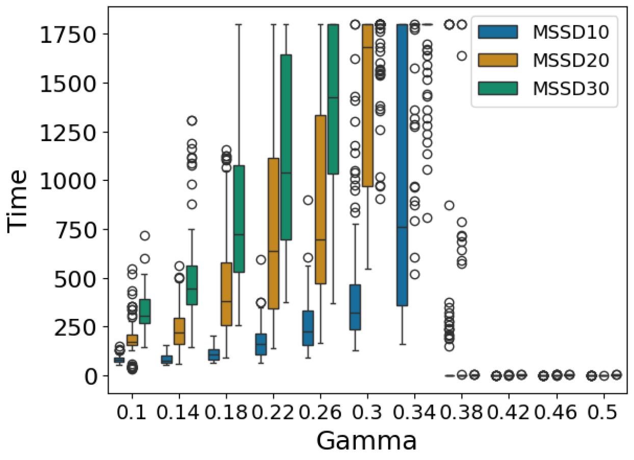
Figure 2: Runtime comparison.

Table 2 shows runtimes for the MSSD models; Sub.O. denotes instances solved within the time limit, but not necessarily optimally. While MSSD10–MSSD30 had few timeouts, MSSD70–MSSD100 had $269$–$300$ timeouts. Table 3 shows individual results for sextile 1 (S1) to sextile 3 (S3) of $\gamma$; the full table is in Appendix A. For all MSSD models both trivial and infeasible problems are solved, see S1 and S3 in Table 3(a). Figure 2 details runtimes for MSSD10–MSSD30 with $\gamma\in[0.1,0.5]$, highlighting the runtime peak for non-trivial instances. The difficulty lies in computing non-trivial counterfactual strategies around S2, where all non-trivial models from MSSD50–MSSD100 timeout, see Table 3(b).

Table 1: Averaged GrepS and BPIC runtime results in seconds for computing counterfactual strategies.

Model	mean(t)	std(t)	min(t)	max(t)	Opt.	Inf.	T.O.
Greps	0.01	0.01	0.01	0.05	90	20	0
BPIC12	0.79	0.94	0.04	4.24	110	0	0
BPIC17	1.00	1.06	0.01	5.01	100	10	0

Table 2: MSSD runtime results in seconds for computing counterfactual strategies.

Model	mean(t)	std(t)	min(t)	max(t)	Opt.	Inf.	T.O.	Sub.O.
MSSD10	56.08	152.35	0.05	T.O.	710	388	2	0
MSSD20	195.77	453.00	0.10	T.O.	707	343	41	9
MSSD30	276.62	556.85	0.14	T.O.	703	320	60	17
MSSD40	412.96	718.68	0.18	T.O.	700	193	207	0
MSSD50	464.38	767.34	0.22	T.O.	700	149	251	0
MSSD60	483.53	788.52	0.24	T.O.	700	123	277	0
MSSD70	485.84	789.70	0.29	T.O.	700	131	269	0
MSSD80	493.91	799.60	0.33	T.O.	700	103	297	0
MSSD90	494.57	799.79	0.36	T.O.	700	100	300	0
MSSD100	494.39	799.90	0.39	T.O.	700	100	300	0

Table 3: MSSD results for selected sextiles of $\gamma$.

	S1 (0, 0.17]				S2 (0.17, 0.33]				S3 (0.33, 0.5]
Model	Opt.	Inf.	T.O.	Sub.	Opt.	Inf.	T.O.	Sub.	Opt.	Inf.	T.O.	Sub.
MSSD10	0	200	0	0	10	188	2	0	200	0	0	0
MSSD20	0	200	0	0	7	143	41	9	200	0	0	0
MSSD30	0	200	0	0	3	120	60	17	200	0	0	0
MSSD40	0	187	13	0	0	6	194	0	200	0	0	0
MSSD50	0	149	51	0	0	0	200	0	200	0	0	0
MSSD60	0	123	77	0	0	0	200	0	200	0	0	0
MSSD70	0	131	69	0	0	0	200	0	200	0	0	0
MSSD80	0	103	97	0	0	0	200	0	200	0	0	0
MSSD90	0	100	100	0	0	0	200	0	200	0	0	0
MSSD100	0	100	100	0	0	0	200	0	200	0	0	0

(a) Categorical results by sextile.

	S1 (0, 0.17]				S2 (0.17, 0.33]				S3 (0.33, 0.5]
Model	mean(t)	std(t)	min(t)	max(t)	mean(t)	std(t)	min(t)	max(t)	mean(t)	std(t)	min(t)	max(t)
MSSD10	39	40	0	128	266	267	73	T.O.	1	0	1	2
MSSD20	92	114	0	684	978	603	126	T.O.	2	0	1	4
MSSD30	159	167	0	567	1352	495	335	T.O.	3	1	2	5
MSSD40	468	585	0	T.O.	1793	59	1144	T.O.	3	1	2	7
MSSD50	743	796	0	T.O.	T.O.	0	T.O.	T.O.	3	1	2	6
MSSD60	847	865	0	T.O.	T.O.	0	T.O.	T.O.	3	1	2	8
MSSD70	858	867	0	T.O.	T.O.	0	T.O.	T.O.	4	1	3	7
MSSD80	899	901	0	T.O.	T.O.	0	T.O.	T.O.	5	1	3	13
MSSD90	900	902	0	T.O.	T.O.	0	T.O.	T.O.	6	1	3	12
MSSD100	900	902	0	T.O.	T.O.	0	T.O.	T.O.	5	1	4	12

(b) Runtime results by sextile, rounded to seconds.

The counterfactual strategies can be used to provide interpretable recommendations to users, which is essential to enable users to follow the recourse suggested by the counterfactual strategy. To this aim, counterfactual strategies are presented in a textual representation highlighting the suggested changes. An example for two states of BPIC12 is given below, where the client is asked not to cancel the loan offer after receiving the first offer but to continue in the process:

State ‘negative’ is reached with probability 0.64.
You can reach ‘negative’ with probability 0.09 as follows:
 In state ‘q9: A_CANCELLED’
  increase probability of action ‘Nabellen offer.’ to 0.89
  decrease probability of action ‘negative’ to 0.07
 In state ‘q27: Nabellen offer.#0’
  increase probability of action ‘O_SENT_BACK’ to 0.81
  decrease probability of action ‘negative’ to 0.0
  decrease probability of action ‘O_CANCELLED’ to 0.0

We summarize our conclusions for Exp1: counterfactual strategies can be efficiently computed for complex MDPs with up to $10\,000$ states and $20\,000$ transitions; these models are significantly larger than models used in current process mining benchmarks but occur in, e.g., MSSD.

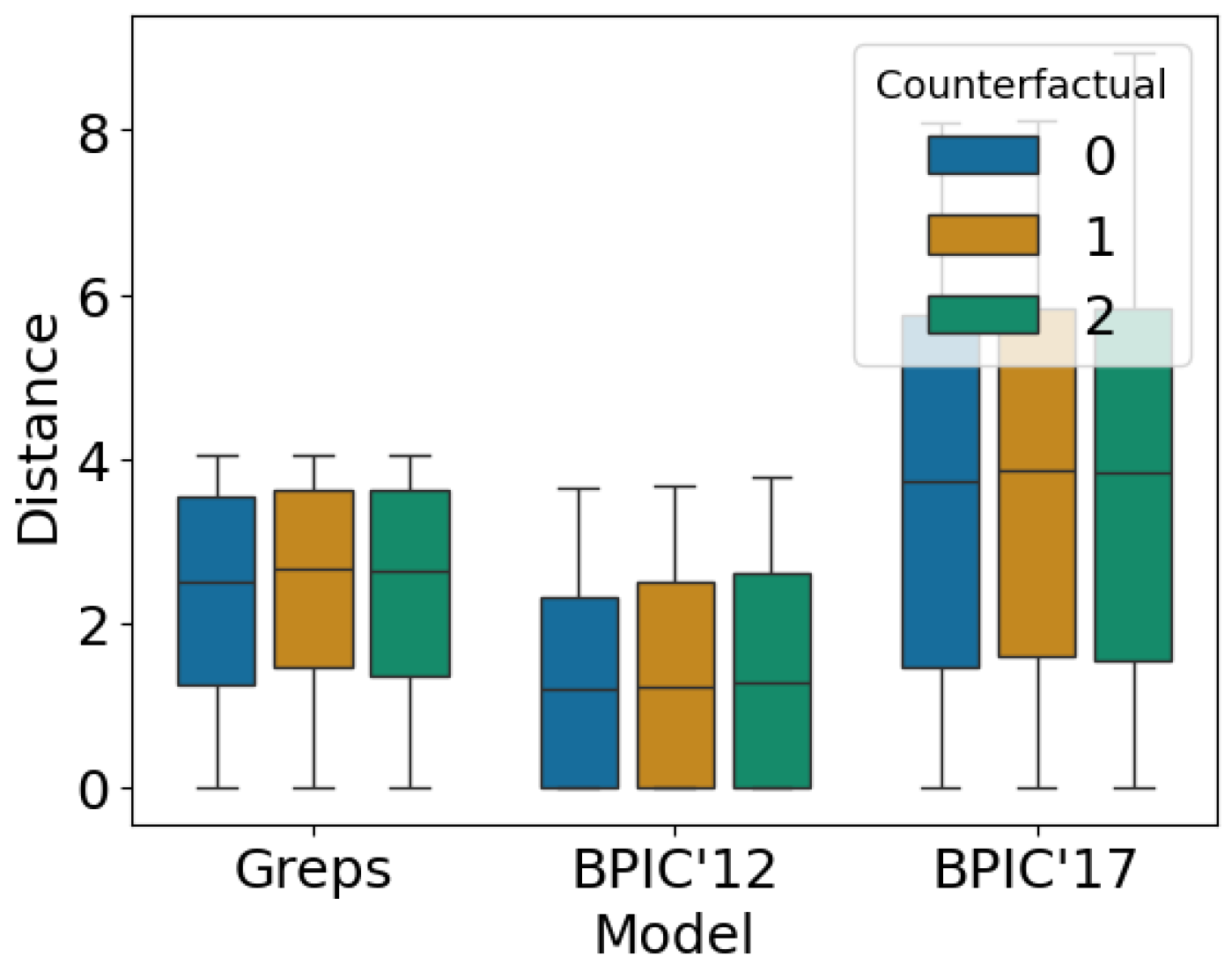
(a) Boxplot over distances from three diverse counterfactual strategies to the initial strategy.

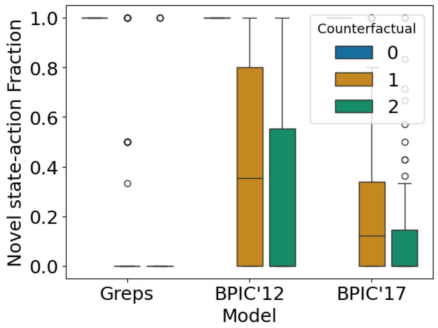
(b) Boxplot showing novel state-action fractions for three diverse counterfactual strategies.

Figure 3: Results for diverse counterfactual strategies.

5.3 Diverse Counterfactuals

In Exp2, we generate a collection of diverse counterfactual strategies for GrepS, BPIC12, and BPIC17 and compare the distance between counterfactual strategies as well as the diversity of the counterfactual strategies. To evaluate diversity, we investigate the fraction of novel state-action pairs, i.e., the actions changed in a counterfactual strategy compared to the initial strategy that were not changed in any previous one.

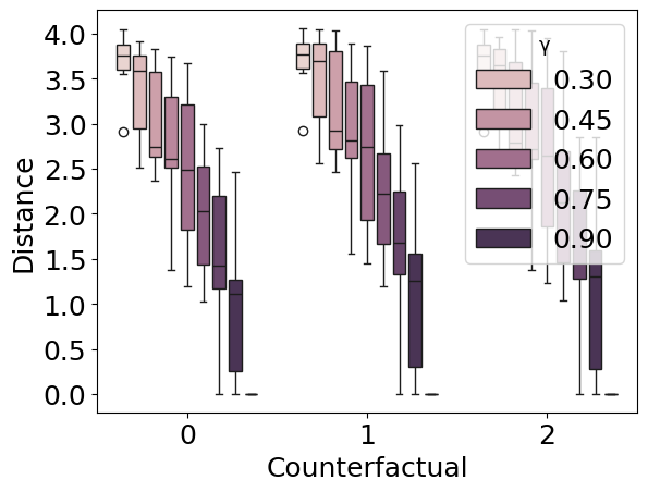
(a) Greps.

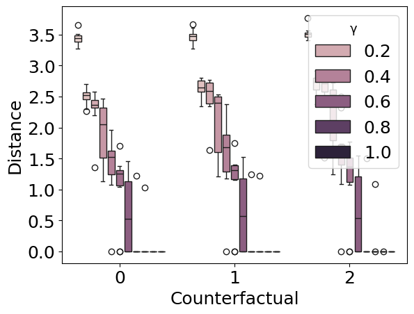
(b) BPIC’12.

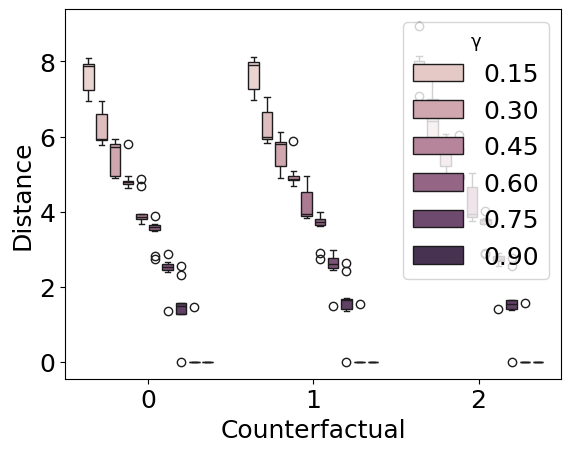
(c) BPIC’17.

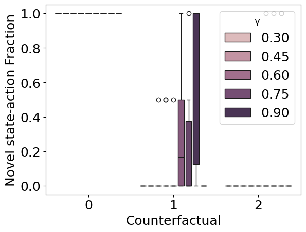
(d) Greps.

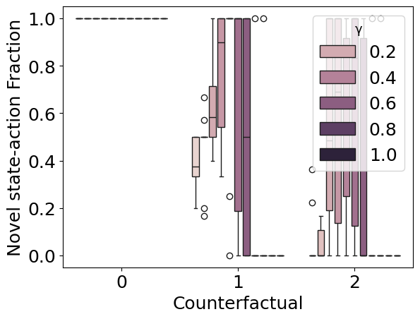
(e) BPIC’12.

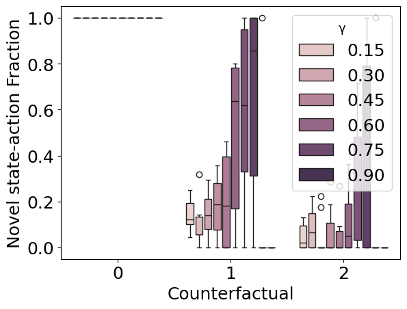
(f) BPIC’17.

Figure 4: Results for diverse counterfactual strategies for each value of $\gamma$.

Figure 3 compares the distance between each generated counterfactual strategy and the initial strategy (Fig. 3(a)), and shows the fraction of novel state-action pairs in each strategy (Fig. 3(b)). While the distance to the initial strategy varies only slightly between consecutive counterfactual strategies, each provides novel recourse strategies. Intermediate values of $\gamma$ offer the largest range of diversity for counterfactual explanations. The individual distances to the initial strategy and the fraction of novel state-action pairs increase with $\gamma$, until the problem is trivially satisfied, see Fig. 4 in Appendix A.

We summarize our conclusions for Exp2: diverse counterfactual strategies can be efficiently computed for the benchmark problems considered. The diverse counterfactual strategies introduce new recourse possibilities while remaining at a short distance to the initial strategy, comparable to the distance of the first counterfactual strategy.

6 Related Work

We discuss related work with respect to stochastic counterfactuals, model repair and synthesis. Balke and Pearl discuss stochastic evaluations of counterfactual queries in their seminal work Balke and Pearl (1994b). Since then, much work on counterfactual explanations has been published, summarized by Guidotti Guidotti (2024). An adaptation for predictive business process monitoring was presented with LORLEY Huang et al. (2021). Notably, MDPs in combination with causal models have been adapted for counterfactual reasoning Tsirtsis et al. (2021); Kazemi et al. (2024). In this line of work, the authors define the transition probabilities of the MDP via structural causal models and then search for a counterfactual path that only diverges in $k$ actions from the given path. In contrast, our work does not assume causal knowledge. We further define counterfactuals over strategies, as opposed to paths in the MDP.

Although both model repair and counterfactuals start with a model and a violated property, these problems aim for different solutions. Model repair considers the problem of adjusting a model to satisfy a desired property Bartocci et al. (2011); Chatzieleftheriou and Katsaros (2018); Chen et al. (2013); Pathak et al. (2015). In contrast, counterfactual strategies do not aim to adjust the underlying model, but rather to propose behavior changes to the user (thus, the transition probabilities of the model remain unchanged).

Recent work on model synthesis for parametric MDPs consider transition probabilities expressed as functions over variables. In this setting, one searches for a parameter valuation such that a given property is satisfied under every strategy Cubuktepe et al. (2017, 2018, 2021). In contrast, our work starts from a fully specified model and a strategy, and we search for a minimal change of the strategy that satisfies the given property.

7 Conclusion

In this work, we introduced counterfactual strategies for Markov decision processes as post-hoc explanations for sequential decision-making tasks. We presented an optimization approach for computing counterfactual strategies and extended it to also optimize for diversity. In extensive experiments on four real-world datasets, we evaluated the generation of diverse counterfactual strategies, showing that counterfactual strategies can be generated within minutes for models significantly larger than current Process Mining benchmarks.

Our work opens several interesting avenues for future work. First, we plan to investigate the complexity of generating counterfactual strategies further, as well as techniques to further reduce the runtime of our approach. Approximations of the optimization problem, such as those based on linearization, e.g., Cubuktepe et al. (2021), promise to reduce the computation time while producing local optimal strategies. Second, it would be interesting to study the problem of generating counterfactual strategies for scenarios where the environment (e.g., the service provider) adapts to counterfactual changes. This will require generalizing our counterfactual strategies from MDPs to Stochastic Games, thus requiring novel theoretical investigations. Finally, it would be interesting to investigate whether our counterfactual strategies result in realistic recourse behaviors, e.g. by measuring similarity to those witnessed in our dataset or by running user studies.

Appendix A Appendix

Table 4: Averaged model overview of each dataset.

	$mean(\text{States})$	$mean(\text{Transitions})$	$max$ Degree
Greps	64.0	76.0	6.0
BPIC’12	129.0	288.0	28.0
BPIC’17	158.0	292.0	19.0
MSSD10	5702.8	11341.5	1952.6
MSSD20	7971.6	16247.5	2794.0
MSSD30	9378.6	19718.0	3397.3
MSSD40	10603.4	22585.8	3857.1
MSSD50	11581.2	25016.5	4249.0
MSSD60	12456.2	27106.1	4612.0
MSSD70	13213.2	28984.2	4918.7
MSSD80	13804.2	30547.4	5171.3
MSSD90	14334.0	31905.5	5403.8
MSSD100	14860.0	33266.0	5622.0

Table 5: GrepS and BPIC runtime results in seconds for quantiles.

	Q1 (0, 0.25]				Q2 (0.25, 0.5]				Q3 (0.5, 0.75]				Q4 (0.75, 1]
Model	mean(t)	std(t)	min(t)	max(t)	mean(t)	std(t)	min(t)	max(t)	mean(t)	std(t)	min(t)	max(t)	mean(t)	std(t)	min(t)	max(t)
Greps	0.0	0.0	0.0	0.0	0.0	0.0	0.0	0.0	0.0	0.0	0.0	0.0	0.0	0.0	0.0	0.1
BPIC’12	1.3	0.8	0.4	3.3	1.2	1.1	0.0	4.2	0.3	0.5	0.0	1.5	0.1	0.2	0.0	1.0
BPIC’17	1.4	1.5	0.0	5.0	1.5	0.8	0.6	3.8	0.8	0.5	0.4	2.2	0.2	0.2	0.0	0.8

Table 6: MSSD results by sextiles.

	S1 (0, 0.17]				S2 (0.17, 0.33]				S3 (0.33, 0.5]				S4 (0.5, 0.67]				S5 (0.67, 0.83]				S6 (0.83, 1]
Model	Opt.	Inf.	T.O.	Sub.	Opt.	Inf.	T.O.	Sub.	Opt.	Inf.	T.O.	Sub.	Opt.	Inf.	T.O.	Sub.	Opt.	Inf.	T.O.	Sub.	Opt.	Inf.	T.O.	Sub.
MSSD10	0	200	0	0	10	188	2	0	200	0	0	0	100	0	0	0	200	0	0	0	200	0	0	0
MSSD20	0	200	0	0	7	143	41	9	200	0	0	0	100	0	0	0	200	0	0	0	200	0	0	0
MSSD30	0	200	0	0	3	120	60	17	200	0	0	0	100	0	0	0	200	0	0	0	200	0	0	0
MSSD40	0	187	13	0	0	6	194	0	200	0	0	0	100	0	0	0	200	0	0	0	200	0	0	0
MSSD50	0	149	51	0	0	0	200	0	200	0	0	0	100	0	0	0	200	0	0	0	200	0	0	0
MSSD60	0	123	77	0	0	0	200	0	200	0	0	0	100	0	0	0	200	0	0	0	200	0	0	0
MSSD70	0	131	69	0	0	0	200	0	200	0	0	0	100	0	0	0	200	0	0	0	200	0	0	0
MSSD80	0	103	97	0	0	0	200	0	200	0	0	0	100	0	0	0	200	0	0	0	200	0	0	0
MSSD90	0	100	100	0	0	0	200	0	200	0	0	0	100	0	0	0	200	0	0	0	200	0	0	0
MSSD100	0	100	100	0	0	0	200	0	200	0	0	0	100	0	0	0	200	0	0	0	200	0	0	0

(a) Categorical results by sextile.

	S1 (0, 0.17]				S2 (0.17, 0.33]				S3 (0.33, 0.5]				S4 (0.5, 0.67]				S5 (0.67, 0.83]				S6 (0.83, 1]
Model	mean(t)	std(t)	min(t)	max(t)	mean(t)	std(t)	min(t)	max(t)	mean(t)	std(t)	min(t)	max(t)	mean(t)	std(t)	min(t)	max(t)	mean(t)	std(t)	min(t)	max(t)	mean(t)	std(t)	min(t)	max(t)
MSSD10	39	40	0	128	266	267	73	T.O.	1	0	1	2	1	0	1	2	1	0	1	2	1	0	1	2
MSSD20	92	114	0	684	978	603	126	T.O.	2	0	1	4	2	0	2	3	2	0	2	4	2	0	2	4
MSSD30	159	167	0	567	1352	495	335	T.O.	3	1	2	5	3	1	2	6	3	0	2	6	3	0	2	5
MSSD40	468	585	0	T.O.	1793	59	1144	T.O.	3	1	2	7	3	1	2	7	3	1	2	7	3	1	2	7
MSSD50	743	796	0	T.O.	T.O.	0	T.O.	T.O.	3	1	2	6	3	1	2	5	3	1	2	8	3	1	2	6
MSSD60	847	865	0	T.O.	T.O.	0	T.O.	T.O.	3	1	2	8	3	1	2	6	3	1	2	10	3	1	2	9
MSSD70	858	867	0	T.O.	T.O.	0	T.O.	T.O.	4	1	3	7	4	1	3	7	4	1	3	7	4	1	3	9
MSSD80	899	901	0	T.O.	T.O.	0	T.O.	T.O.	5	1	3	13	5	1	4	14	5	1	3	11	5	1	3	8
MSSD90	900	902	0	T.O.	T.O.	0	T.O.	T.O.	6	1	3	12	6	2	4	14	5	1	3	11	6	1	4	11
MSSD100	900	902	0	T.O.	T.O.	0	T.O.	T.O.	5	1	4	12	6	1	4	10	5	1	4	11	5	1	4	12

(b) Runtime results by sextile, rounded to seconds.

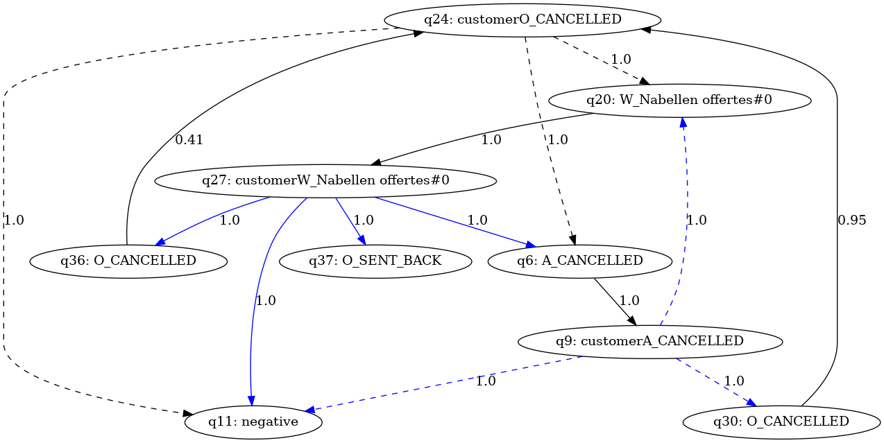
Figure 5: Comparison of two counterfactual strategies for BPIC’12. We only depict states that are close to a state where any counterfactual strategy differs from the initial strategy. Actions are colored blue if the first counterfactual strategy differs from the initial strategy for that action, and are dashed if the second counterfactual strategy differs.

A.1 Further details on experimental setup

We preprocess the datasets following the literature (for GrepS Kobialka et al. [2024], for BPIC12 Bautista et al. [2012], for BPIC17 Kobialka et al. [2023]; Rodrigues et al. [2017], and for MSSD Johnsen et al. [2025]). In the preprocessing of the datasets, we removed irregular behavior, filtered unused events, and massaged event names to improve the resulting models, e.g. we added the count of the current offer in BPIC’12 to the event name to differentiate consecutive offers. For MSSD, We adapt the preprocessing by Johnsen et al. for counterfactuals by ignoring weights and real-time information, and introduce a negative state if the listening sessions have less than 15 songs, and otherwise a positive state.

Due to the complexity of MSSD, we generate models over multiples of $10\%$ of the $10\,000$ listening sessions For each multiple of $10\%$, we build ten models each with a random subset from MSSD. The generated models have between $64$ and $15\,000$ states, $76$ – $33\,000$ transitions and a maximal out degree between $6$ and $5\,622$, as shown in Table 4. To differentiate between datasets and models, we denote models in bold, i.e. MSSD10 denotes a model for 1000 listening sessions.

We implemented our evaluation framework in Python 3.10.12, using Gurobi 11.0.3. For model construction, we use the jAlergia implementation of the automata learning algorithm Alergia Carrasco and Oncina [1994], accessed through the Python automata learning library AAlpy, version 1.4.1 Muškardin et al. [2022]. The generated benchmark set and code is available online. We deploy the executions on a workstation with 128 GB memory and a 64-core AMD EPYC processor. We restrict Gurobi to use one core, limit its memory to $2.5\text{\,}\mathrm{GB}$ of RAM, and the computation time to $1800$ seconds.

A.2 Extended results

We present extended results omitted in the main paper. Table 5 presents the run times for computing counterfactual strategies for each $\gamma$-quantile for Greps, BPIC’12 and BPIC’17.

Table 6 presents categorical and run time results for each $\gamma$-sextile for computing counterfactual strategies for MSSD.

References

- Baier and Katoen [2008] Christel Baier and Joost-Pieter Katoen. Principles of Model Checking. MIT press, 2008.
- Balke and Pearl [1994a] Alexander Balke and Judea Pearl. Counterfactual probabilities: Computational methods, bounds and applications. In Uncertainty in artificial intelligence, pages 46–54. Elsevier, 1994.
- Balke and Pearl [1994b] Alexander Balke and Judea Pearl. Probabilistic evaluation of counterfactual queries. In Proc. 12th National Conference on Artificial Intelligence (AAAI), pages 230–237. AAAI Press / The MIT Press, 1994.
- Bartocci et al. [2011] Ezio Bartocci, Radu Grosu, Panagiotis Katsaros, CR Ramakrishnan, and Scott A Smolka. Model repair for probabilistic systems. In Proc. 17th International Conference on Tools and Algorithms for the Construction and Analysis of Systems (TACAS 2011), pages 326–340. Springer, 2011.
- Bautista et al. [2012] Arjel D Bautista, Lalit Wangikar, and Syed M Kumail Akbar. Process mining-driven optimization of a consumer loan approvals process. BPI Challenge, 2012.
- Billionnet et al. [2016] Alain Billionnet, Sourour Elloumi, and Amélie Lambert. Exact quadratic convex reformulations of mixed-integer quadratically constrained problems. Mathematical Programming, 158(1):235–266, 2016.
- Bove et al. [2023] Clara Bove, Marie-Jeanne Lesot, Charles Albert Tijus, and Marcin Detyniecki. Investigating the intelligibility of plural counterfactual examples for non-expert users: an explanation user interface proposition and user study. In Proc. 28th International Conference on Intelligent User Interfaces, pages 188–203. ACM, 2023.
- Boyd and Vandenberghe [2004] Stephen P. Boyd and Lieven Vandenberghe. Convex Optimization. Cambridge University Press, 2004.
- Brost et al. [2019] Brian Brost, Rishabh Mehrotra, and Tristan Jehan. The music streaming sessions dataset. In The World Wide Web Conference, pages 2594–2600, 2019.
- Carrasco and Oncina [1994] Rafael C Carrasco and José Oncina. Learning stochastic regular grammars by means of a state merging method. In International Colloquium on Grammatical Inference, pages 139–152. Springer, 1994.
- Chatzieleftheriou and Katsaros [2018] George Chatzieleftheriou and Panagiotis Katsaros. Abstract model repair for probabilistic systems. Information and Computation, 259:142–160, 2018.
- Chen et al. [2013] Taolue Chen, Ernst Moritz Hahn, Tingting Han, Marta Kwiatkowska, Hongyang Qu, and Lijun Zhang. Model repair for Markov decision processes. In 2013 International Symposium on Theoretical Aspects of Software Engineering, pages 85–92. IEEE, 2013.
- Cubuktepe et al. [2017] Murat Cubuktepe, Nils Jansen, Sebastian Junges, Joost-Pieter Katoen, Ivan Papusha, Hasan A. Poonawala, and Ufuk Topcu. Sequential convex programming for the efficient verification of parametric MDPs. In Proc. 23rd International Conference on Tools and Algorithms for the Construction and Analysis of Systems (TACAS 2017), volume 10206 of LNCS, pages 133–150. Springer, 2017.
- Cubuktepe et al. [2018] Murat Cubuktepe, Nils Jansen, Sebastian Junges, Joost-Pieter Katoen, and Ufuk Topcu. Synthesis in pMDPs: A tale of 1001 parameters. In International Symposium on Automated Technology for Verification and Analysis, pages 160–176. Springer, 2018.
- Cubuktepe et al. [2021] Murat Cubuktepe, Nils Jansen, Sebastian Junges, Joost-Pieter Katoen, and Ufuk Topcu. Convex optimization for parameter synthesis in MDPs. IEEE Transactions on Automatic Control, 67(12):6333–6348, 2021.
- Gajcin and Dusparic [2024] Jasmina Gajcin and Ivana Dusparic. Redefining counterfactual explanations for reinforcement learning: Overview, challenges and opportunities. ACM Computing Surveys, 56(9):1–33, 2024.
- Garey and Johnson [1979] Michael R Garey and David S Johnson. Computers and Intractability: A Guide to the Theory of NP-Completeness. W. H. Freeman, 1979.
- Guidotti [2024] Riccardo Guidotti. Counterfactual explanations and how to find them: literature review and benchmarking. Data Mining and Knowledge Discovery, 38(5):2770–2824, 2024.
- Huang et al. [2021] Tsung-Hao Huang, Andreas Metzger, and Klaus Pohl. Counterfactual explanations for predictive business process monitoring. In European, Mediterranean, and Middle Eastern Conference on Information Systems, pages 399–413. Springer, 2021.
- Johnsen et al. [2025] Einar Broch Johnsen, Paul Kobialka, Andrea Pferscher, and Silvia Lizeth Tapia Tarifa. Nudging strategies for user journeys: Take a path on the wild side. In Real Time and Such - Essays Dedicated to Wang Yi to Celebrate His Scientific Career, volume 15230 of LNCS, pages 42–63. Springer, 2025.
- Kazemi et al. [2024] Milad Kazemi, Jessica Lally, Ekaterina Tishchenko, Hana Chockler, and Nicola Paoletti. Counterfactual influence in Markov decision processes. arXiv preprint arXiv:2402.08514, 2024.
- Kobialka et al. [2022] Paul Kobialka, Silvia Lizeth Tapia Tarifa, Gunnar Rye Bergersen, and Einar Broch Johnsen. Weighted games for user journeys. In Proc. 20th International Conference Software Engineering and Formal Methods (SEFM 2022), volume 13550 of LNCS, pages 253–270. Springer, 2022.
- Kobialka et al. [2023] Paul Kobialka, Felix Mannhardt, Silvia Lizeth Tapia Tarifa, and Einar Broch Johnsen. Building user journey games from multi-party event logs. In Proc. Workshop on Event Data and Behavioral Analytics (EdbA 2022), volume 468 of Lecture Notes in Business Information Processing, pages 71–83. Springer, 2023.
- Kobialka et al. [2024] Paul Kobialka, Silvia Lizeth Tapia Tarifa, Gunnar Rye Bergersen, and Einar Broch Johnsen. User journey games: Automating user-centric analysis. Software & Systems Modeling, 23(3):605–624, 2024.
- Leo et al. [2019] Martin Leo, Suneel Sharma, and Koilakuntla Maddulety. Machine learning in banking risk management: A literature review. Risks, 7(1):29, 2019.
- Levin and Peres [2017] David A Levin and Yuval Peres. Markov Chains and Mixing Times, volume 107. American Mathematical Soc., 2017.
- Mao et al. [2016] Hua Mao, Yingke Chen, Manfred Jaeger, Thomas D. Nielsen, Kim G. Larsen, and Brian Nielsen. Learning deterministic probabilistic automata from a model checking perspective. Machine Learning, 105(2):255–299, 2016.
- Molnar [2020] Christoph Molnar. Interpretable Machine Learning. Lulu.com, 2020.
- Mothilal et al. [2020] Ramaravind K Mothilal, Amit Sharma, and Chenhao Tan. Explaining machine learning classifiers through diverse counterfactual explanations. In Proc. 2020 Conference on Fairness, Accountability, and Transparency, pages 607–617. ACM, 2020.
- Muškardin et al. [2022] Edi Muškardin, Bernhard K Aichernig, Ingo Pill, Andrea Pferscher, and Martin Tappler. AALpy: an active automata learning library. Innovations in Systems and Software Engineering, 18(3):417–426, 2022.
- Pathak et al. [2015] Shashank Pathak, Erika Ábrahám, Nils Jansen, Armando Tacchella, and Joost-Pieter Katoen. A greedy approach for the efficient repair of stochastic models. In NASA Formal Methods Symposium, pages 295–309. Springer, 2015.
- Rodrigues et al. [2017] Ariane M B Rodrigues, Cassio F P Almeida, Daniel D G Saraiva, Georges M Spyrides, Guilherme Varela, Gustavo M Krieger, Leila F Dantas, Mauricio Lana, Odair E Alves, Rafael Franca, A Q Neira, Sonia F Gonzalez, William P D Fernandes, Simone D J Barbosa, Marcus Poggi, and Helio Lopes. Stairway to value: Mining a loan application process. BPI Challenge, page 30, 2017.
- Russell [2019] Chris Russell. Efficient search for diverse coherent explanations. In Proc. Conference on Fairness, Accountability, and Transparency, pages 20–28. ACM, 2019.
- Teinemaa et al. [2019] Irene Teinemaa, Marlon Dumas, Marcello La Rosa, and Fabrizio Maria Maggi. Outcome-oriented predictive process monitoring: Review and benchmark. ACM Transactions on Knowledge Discovery from Data (TKDD), 13(2):1–57, 2019.
- Tsirtsis et al. [2021] Stratis Tsirtsis, Abir De, and Manuel Rodriguez. Counterfactual explanations in sequential decision making under uncertainty. Advances in Neural Information Processing Systems, 34:30127–30139, 2021.
- van Dongen [2012] Boudewijn van Dongen. BPI Challenge, 2012.
- van Dongen [2017] Boudewijn van Dongen. BPI Challenge, 2017.