Structured coalescents, coagulation equations and multi-type branching processes
Abstract.
We consider the genealogy of a structured population consisting of colonies. Individuals migrate between colonies at a rate that scales with a positive parameter . Within a colony, pairs of ancestral lineages coalesce at a constant rate, i.e. as in Kingman coalescent. We start this multi-type coalescent with single lineages distributed among the colonies. We consider two regimes: the critical sampling regime (case ) and the large sampling regime (case ). In this setting, we study the asymptotic behaviour, as , of the vector of empirical measures, whose -th component keeps track at each time of the blocks present at colony , and of the initial location of the lineages composing each blocks. We show that, in the proper time-space scaling (small times), the process of empirical measures converges to the solution of a -dimensional coagulation equation. In the critical sampling regime, its solution admits a stochastic representation in terms of a multi-type branching process, and in the large sampling regime in terms of the entrance law of a multi-type Feller diffusion.
MSC 2020. Primary: 60J90; 60G57 Secondary: 60J95; 60B10; 60J80; 35Q92
Keywords. Structured coalescent; coagulation equations; multi-type branching processes; multi-type Feller-diffusions
1. Introduction
Coalescents, branching processes, and coagulation equations represent three fundamental approaches for modeling the dynamics of general interacting particle systems. Each of these captures a distinct yet interconnected facet of stochastic evolution: coalescents describe the merging of ancestral lineages backward in time; branching processes model population growth and reproduction mechanisms forward in time; and coagulation equations provide deterministic approximations for the evolution of cluster sizes in systems undergoing mass-conserving mergers.
The relationship between these models is both theoretically rich and practically significant. For instance, the interplay of the evolution of block-sizes in Kingman’s coalescent [9] and critical branching processes is well known, as both the mean-field limit of the former and the law of the latter solve a Smoluchowski-type coagulation equation (see for example [2, 5, 3]). In this work, we extend this connection to a multi-type setting, where multiple interacting types (or subpopulations) are involved.
Our starting point is a coalescent model drawn from a subclass of multi-type -coalescents [8], commonly referred to as (mainland-)island models. These models describe structured populations partitioned into colonies (or islands), where individuals typically remain within their colony for life, with occasional migration events between colonies. In our formulation, colonies are represented by colors, and only pairs of blocks that share the same color may merge (as in Kingman’s coalescent [9]), while blocks can change color through migration.
This general framework is closely related to the classical structured coalescent [11] but, crucially, diverges significantly in its treatment of migration rates in the large population limit (). Standard scaling regimes assume either strong migration () or weak migration (). In contrast, we focus on an intermediate or moderate migration regime, where for some . Simultaneously, we consider varying sample sizes of order with . For notational convenience, we denote the order of the migration rate by , and the corresponding sample size by , allowing us to interpret the samples as drawn from an effectively infinite population, dependent on the migration rate.
In this setting, we investigate the asymptotic behavior of the vector of empirical measures as at small times, whose -th component keeps track of the blocks of color at time and of the initial coloring of the integers composing each of these blocks. We prove that, under suitable time-space scaling, this vector converges to the solution of a multi-dimensional Smoluchowski-type coagulation equation.
This result parallels the findings of [10], which examined a different framework known as nested coalescents, modeling both the ancestry of species and the ancestry of genes within each species. Although our coagulation equation is simpler, lacking their transport term, it may give rise to degenerate initial conditions depending on the initial sample size. Nevertheless, we show that, as in the single-type case, the solution to our coagulation equation corresponds either to the law of a critical multi-type branching process, or to the entrance law of a multi-type Feller diffusion, depending on the initial sample size.
2. Model and main results
In this section we formalize the definition of the structured coalescent that will be the object of our analysis and we state our main results.
2.1. The model
We consider a prototype model for the genealogies of a large population divided into colonies, where will remain fixed all along the manuscript. The model takes the form of a structured coalescent that evolves according to the following principles. Within a colony, blocks coalesce as in Kingman’s coalescent (i.e. at a constant rate per pair of blocks), while blocks can also migrate between colonies at rates proportional to a scaling parameter . The aim of this article is to analyze the effect of sample size in the corresponding ancestral structures, at small times, as .
Let us now formalize the previous description. Each individual in the population is identified by a unique number in ; each colony is identified by a unique number in , which we will often refer to as a color. The state of the system is encoded by a structured partition as defined below.
Definition 2.1 (Structured/colored partition).
Let . We refer to the elements of as colored (positive) integers. We say that is a coloring of if for some . We refer to as a colored partition of a coloring of if are disjoint (possibly empty) collections of non-empty subsets of and is a partition of ; we call the elements of blocks of color . If is a coloring of , we denote by the set of all colored partitions of and by the set of all colored partitions of some coloring of . We equip and with the discrete topology.
Example 2.2.
is a coloring of with colors.
is a colored partition of with blue blocks and 1 green block.
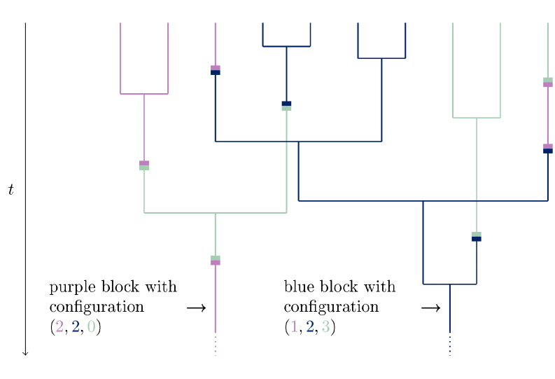
Now, we describe the anticipated multi-type coalescent as a Markov process on the set of colored partitions. Fix . Let be a primitive matrix and . The multi-type coalescent is the continuous-time Markov chain on which is characterized by the following dynamics (see Fig. 1):
-
(1)
At time , start with a coloring of . The partition is the set of singletons whose coloring coincides with the coloring of . For instance, for the coloring of in Example 2.2,
-
(2)
Each block changes its color from to at rate . For instance
-
(3)
For every in , each pair of blocks of color coalesce into a single block of color at rate . For instance
Pairs of different colors do not coalesce.
If we envision the coalescent as a random ultrametric tree, the color of a block and its internal coloring can be interpreted as follows. The color of a given block at time is the position of a lineage. The internal coloring provides the labels and colors of the leaves supported by this lineage units of time in the past (see Fig. 1).
Assumption 2.3.
Let be the number of blocks of color at time . There is a vector , such that, for each ,
Since the matrix is primitive, it follows that it admits a unique stationary distribution, which we denote by .
2.2. The empirical measure
In this work we will focus on the asymptotic properties of a functional of the coalescent , which will code for the colony sizes, but also for the color-configurations within blocks. To encode this information, we will need a few definitions.
We will say that the internal coloring of a block is if and only if the block contains elements of color , elements of color etc.
For instance, the internal coloring of the blue block
is .
For every time , we define the empirical measure as the element of such that
In words, is the number of lineages at time located in colony carrying leaves of color etc. As anticipated at the beginning of the section, our aim is to understand the interplay between the sampling size and the scale at which migrations (change of color) occur in the model. In our analysis, we will distinguish between the two regimes depending on the asymptotic behavior of . More precisely, we consider:
-
(1)
The critical sampling regime:
-
(2)
The large sampling regime:
To avoid unnecessary case distinctions when scaling blocks, we will use the notation
| (2.1) |
Note that in both regimes
| (2.2) |
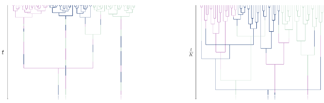
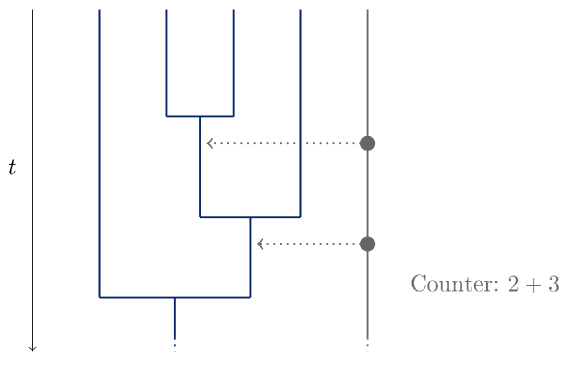
In the critical sampling regime, the rates of migration and coalescence events will both be of the same order as long as the total number of blocks remains of order . In contrast, in the large sampling regime, coalescence events will dominate the dynamics as long as the total number of blocks is of a higher order than , and only when the total number of blocks reaches order will coalescence events and migrations synchronize on the same time scale. We will therefore slow down time by , so that the time frame in which coalescence dominates the dynamics is very short, and hence the strengths of migration and coalescence equilibrate very quickly (see Fig. 2 for an illustration of the time scaling). As a consequence, in the large sampling regime, blocks will quickly become very large, and we will therefore need to introduce an appropriate space scaling. More precisely, we will consider the rescaled measure valued process valued in equipped with weak topology as
2.3. Convergence
In this section we state the two main results concerning the convergence of the empirical measures as . Let us anticipate that our results will differ substantially depending on the parameter regime under consideration.
We start by introducing some notation. If we denote by their convolution, i.e.
In addition, if and is integrable with respect to , we set
If the involved measures have discrete support, the integrals can, as usual, be understood as sums.
Now we state our main convergence result in the critical regime.
Theorem 2.4 (Critical sampling).
Assume that as . If Assumption 2.3 holds, then weakly converges, as , to the solution of the -dimensional discrete coagulation equation
| (2.3) | ||||
| (2.4) |
for all , and , where denotes the canonical basis of .
The dynamics of the coagulation equation is very intuitive. When two blocks coalesce, the resulting block configuration is the sum of the block configurations of the coalescing blocks; hence the convolution. Moreover, whenever a block with a given configuration merges with another block, we lose that configuration. The remaining sum is due to migration: we gain a block configuration in colony whenever a block with that configuration migrates from another colony to colony ; we lose a block configuration whenever a block with that configuration migrates from colony to another colony . The initial condition is due to the fact that at time there are approximately singletons in colony .
The next theorem covers the large sampling case.
Theorem 2.5 (Large sampling).
Assume that as . If Assumption 2.3 holds, then weakly converges, as , to the weak solution of the -dimensional continuous coagulation equation
| (2.5) | |||
| (2.6) |
Remark 2.6.
By weak solution, we mean that for
2.4. Stochastic representation
In this section we provide stochastic representations to the coagulation equations obtained in the previous section. We provide here the derivation only on the large sampling case; the critical sampling case will be treated analogously in Appendix A. Therefore, throughout this section, we assume that as .
Let be the solution of the continuum coagulation equation (2.5) under (2.6). Define
A direct computation shows that solves the multi-dimensional ODE
where
We identify as the Laplace exponent of the -CSBP, or equivalently the -dimensional Feller diffusion solution of the SDE
| (2.7) |
where is a standard -dimensional Brownian motion. Thus, for every , we have
| (2.8) |
Let be the entrance law of the process from state , i.e.
Using standard arguments one can deduce from (2.8) that for
But recall that
We can then invert the Laplace transform and get the following result.
Theorem 2.7.
For the critical sampling, we will prove the following analogous result in Appendix A.
Theorem 2.8.
If we choose , where is the equilibrium measure with respect to the migration matrix, the solution of the coagulation equation of (2.3) with initial condition (2.4) admits the stochastic representation
where denotes a continuous-time multi-type branching process, such that a particle of color
-
•
branches and dies at rate .
-
•
makes a transition from to at rate .
2.5. Proof strategy
The remainder of the manuscript is devoted to the proofs of Theorems 2.4 and 2.5. In Section 3.1, we characterize the generator of the process of empirical measures and establish its convergence in a precise sense. In Section 3.4 we establish a coupling allowing us to compare the number of blocks in our multi-type coalescent to the number of blocks in Kingman’s coalescent; the resulting bounds will play an important role in later sections. In Section 4, we prove the tightness of the sequence of empirical measures and characterize its accumulation points. Finally, in Section 5, we complete the proofs of Theorems 2.4 and 2.5, offering further insight into the role of the initial condition in the large sampling regime (i.e. Eq. (2.4)).
3. Convergence of the generators and Kingman bounds
In this section we describe the action of the infinitesimal generator of the process of empirical measures on a special class of functions. We will use to derive properties of the process . In the second half of this section we will prove the convergence as of the generators , in an appropriate sense.
3.1. The action of the generator
Let be the set of real-valued functions on of the form
| , | (3.1) |
for some and with for , where
To describe the action of the generator of the process of empirical measures on functions in , we write
where the operators and account for the contributions of migrations and coalescences, respectively. For the migration part, recall that any block-configuration present in colony migrates to colony at rate , which has the effect on of adding to coordinate a mass at and removing from coordinate a mass at (see Fig. 3 (right)). This yields
| (3.2) |
where .
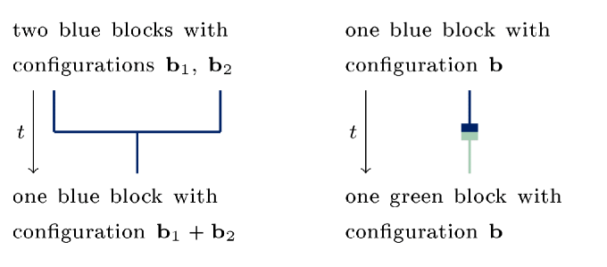
For the coalescent part, recall that any pair of block configurations , present in colony coalesces at rate , which has the effect on of adding to the coordinate a mass at and removing from the coordinate a mass at and (see Fig. 3 (left)). Distinguishing between the cases where and yields
| (3.3) |
where .
3.2. Useful bounds
The next result provides bounds for some functionals of the measures , which will be used in Section 4 (see proof of Lemma 4.8) and Section 5 (see proof of Proposition 5.1).
Lemma 3.1.
Proof.
We begin with the proof of (3.4). Note that for and , we have
Hence . Moreover, Eq. (3.2) yields . To deal with coalescences, we group block-configurations in sets of the form , and we use Eq. (3.1) together with the inequality , to obtain
Recalling the definition of yields
Using this and Fubini yields Thus, setting , it then follows from Dynkin’s formula that
Moreover, at time we have
and (3.4) follows.
3.3. Convergence of the generators
In this section, we will prove a uniform convergence result for the generator . Since our final goal is to prove the convergence of the measures toward the solution of the coagulation equation (2.3) (resp. (2.5)), the generator of the limiting object should be given formally by
where denotes the solution of Eq. (2.3) (resp. Eq. (2.5)) with initial value . For functions , a straightforward calculation shows that
The next result formalises the announced convergence result.
Proposition 3.2.
For any with bounded second order partial derivatives and with , for , there is a constant such that
| (3.6) |
Proof.
Let us start with the migration part of the generator. A second order Taylor’s expansion for at yields
where for a constant depending only on the supremum of and the second order partial derivatives of . Plugging this into Eq. (3.2) yields
and .
Similarly, for the coalescence part of the generator, we use a second order Taylor expansion at , to obtain
for a constant depending only on the supremum of and the second order derivatives of . Plugging this into Eq. (3.1), we obtain
The result follows combining the bounds for the error arising from the migration and from the coalescent parts. ∎
3.4. Comparison results
In this section we will provide a comparison result between the total number of blocks in the multi-type coalescent and two Kingman coalescents. This result will allow us to get a hand on the order of magnitude of the colony sizes.
3.4.1. The coupling
Let be the process that accounts for the total number of blocks in , i.e.
We start this section with the announced coupling result.
Lemma 3.3 (Coupling to Kingman).
There is a coupling between the vector-valued process and other two processes and distributed as the block-counting processes of Kingman coalescents with merger rates per pair of blocks and , respectively, such that
and .
Proof.
We first prove deterministic inequalities that will help us to compare the coalescence rates of the three processes. We claim that for any with ,
| (3.7) |
Indeed, for with , Cauchy-Schwartz inequality yields
and the claimed lower bound for follows. The upper bound is a direct consequence of the inequality .
Equipped with (3.7) we construct the announced coupling. We start , and such that .
Assume that we have constructed them up to the -th transition (transitions refer to the times at which at least one of the three processes makes a jump; we consider time as the -th transition), which brings , and respectively to states satisfying and . The next transition is then constructed as follows. We define
and . We refer to and as coalescence rates of , , , respectively. Then after an exponential time with parameter
-
(1)
with probability a migration event takes place (affecting only ). More precisely,
(and ) remain unchanged.
-
(2)
with probability a coalescence event takes place. The coalescence will always produce a transition among states whose coalescence rate is equal to ; the state associated with the second highest coalescence rate will only be modified with some probability and only then will the state with the lowest coalescence rate be affected with some probability.
There are possible cases to consider that correspond to the different orderings of the coalescence rates of . We explain in detail one case; the others are analogous. We consider the case where . In this case, the transition
takes place. In addition, with probability the state transitions. The transition affects only one of its coordinates; it is the -th coordinate with probability , in which case the transition
takes place. Finally, only if changes, the transition
occurs with probability ; otherwise, remains unchanged.
As soon as goes below , we continue to carry out the coupling between and ; the process can then be further constructed independently.
Note that, thanks to (3.7), if , then . Similarly, if , then . This, together with the fact that the transitions only decrease the size of the affected states by one, implies that the transitions will preserve the ordering . The proof is achieved by noticing that the so-constructed processes have the desired distributions. ∎
3.4.2. Kingman bounds
The following result on Kingman’s coalescent will be helpful in many proofs. We provide here a short proof for completeness.
Lemma 3.4 (Moment bounds).
Let be the block-counting process of a Kingman coalescent with merger rate , which started with blocks at time . Then, for any , we have
Proof.
Let denote the generator of and . Clearly,
Using that, for , and , we get
Combining this with Dynkin’s formula and Jensen inequality, we get
Setting , the previous inequality implies that
Dividing both sides by and integrating both sides of the resulting inequality between and and rearranging terms yields the result. ∎
4. Tightness and characterization of accumulation points
In this section we will prove the tightness of the sequence and characterize its accumulation points, paving the way to the desired convergence result.
4.1. Tightness
The next proposition states the tightness of and is the main result of this section.
Proposition 4.1.
Let in the critical sampling case and (with fix, but arbitrary) in the large sampling case. For any , the sequence of measure-valued processes is tight in , where stands for the weak topology,
4.1.1. The proof strategy
To prove Proposition 4.1, we will show that the sequence of product measures
is tight. The tightness of the sequence will then follow from the continuous mapping theorem (see [4, Thm. 2.7]).
With this in mind, we introduce the following notation. Let denote the space of functions of the form
for some and for , . According to the Stone-Weierstrass theorem, is dense in the set of continuous functions vanishing at infinity.
Our proof of the tightness of in follows a standard line of argumentation (see e.g. [6, 14, 13]), which, in our setting, amounts to proving that the following three conditions are met.
(P1) For every function , the sequence is tight in .
(P2) .
(P3) Any accumulation point of in belongs to
.
The strategy is analogous to the one used in [10, Thm. 7.4]), but they use a version of (P3) considering accumulation points in , where stands for the vague topology. The fact that these three conditions imply the tightness of follows from [14, Thm. 1.1.8] (see Remark 4.2 below). According to Roelly’s criterium (see [12]), condition (P1) already implies tightness in , where stands for the vague topology. Conditions (P2) and (P3) allow one to go from vague convergence to weak convergence (see [14, Lemma. 1.1.9]).
Remark 4.2.
Property (P2) slightly differs from the property stated in [14, Thm. 1.1.8], which reads as
| (4.1) |
where is a function satisfying that To see that (P2) is a stronger condition, note that Markov’s inequality implies that, for all ,
In particular, we have
Another application of Markov’s inequality shows that, under (P2), condition (4.1) holds.
Remark 4.3.
In view of our proof strategy, it will be useful to notice that (recall (3.1)), we have for as above and
| (4.2) |
4.1.2. A bound on the quadratic variations
In the next lemma, an important role is played by the functions , , defined via
Lemma 4.4 (Quadratic variation).
Let in the critical sampling case and in the large sampling case. For any , and , there is a constant and decreasing processes and satisfying that
and such that for any
| (4.3) | ||||
| (4.4) |
where stands for the quadratic variation at time .
Proof.
4.1.3. On the proof of (P1)
To prove (P1), we will use a classic result of Aldous and Rebolledo (see [1], [7]), which consists of two ingredients; the first is the content of the next lemma.
Lemma 4.5.
In the critical (resp. large) sampling case, for every fix (resp. ), the sequence is tight.
Proof.
The second ingredient is provided by the following result.
Lemma 4.6.
Let in the critical sampling case and in the large sampling case. Let , , and . Define
Then, for any and any pair of stopping times such that , there are constants such that
In particular, the two quantities are bounded from above by a function of that goes to as .
Proof.
Lemma 4.7 ((P1)).
Let in the critical sampling case and in the large sampling case. For every function and , the sequence is tight in .
4.1.4. On the proof of (P2)
Now we proceed with the proof of condition (P2).
Lemma 4.8 ((P2)).
Let in the critical sampling case and in the large sampling case. We have
Proof.
For the critical sampling, we would like to make use of Eq. (3.4) from Lemma 3.1. To that end, once again since , we find (with abuse of notation)
Note that on the left hand side we integrate against the 2-Norm on , whereas on the right hand side we integrate against the 2-Norm on . Further, since the sum of the squares is smaller than the square of the sum:
Last, since the block sizes are only increasing over time, and again the sum of the squares is smaller than the square of the sum, Eq. (3.4) already yields
because we assumed for all throughout the section. Since , we conclude:
The proof for the large sampling follows the same general idea, only that here, we make use of Eq. (3.5). More explicitly, this time we find (again with abuse of notation)
Note that (again) on the left hand side we integrate against the 2-Norm on , whereas on the right hand side we integrate against the 2-Norm on . For the first expectation on the right hand side, we again use that the sum of squares is smaller than the square of the sum and that blocks are only increasing over time:
We may therefore apply Eq. (3.5) to find
| (4.5) |
For the second expectation, since the number of blocks is decreasing over time, we first find
Moreover, according to Lemmas 3.3 and 3.4
| (4.6) |
Combining Eq. (4.5) and Eq. (4.6), we arrive at
4.1.5. On the proofs of (P3) and Proposition 4.1
In this section we prove condition (P3) and conclude the proof of Proposition 4.1
Lemma 4.9 ((P3)).
Let in the critical sampling case and in the large sampling case. Any accumulation point of in belongs to .
Proof.
We start with the critical sampling case. Let be an accumulation point of the sequence in . By a slight abuse of notation we denote by the subsequence converging to . Recall that
-
•
a migration from colony to colony moves a single point measure with a mass of from to
-
•
a coalescence removes two point measures each with a mass of and adds another point measure, also with a mass of .
Using this and that , it follows that
It follows that .
Let us now consider the large sampling case. Similarly as before, let be an accumulation point of the sequence in . By a slight abuse of notation we denote by the subsequence converging to . This time we obtain
and the result follows using Lemma 3.3 and that, for the Kingman coalescent started with infinitely many lines, converges almost surely as to a positive constant. ∎
We now have all the ingredients to prove the tightness of .
4.2. Characterization of the accumulation points
We conclude with the main result of this section, characterizing the accumulation points of the sequence of vectors of measures :
Proposition 4.10.
Let in the critical sampling case and in the large sampling case. Consider an accumulation point of . For every with , we define
where is the projection to the -th coordinate and , for . Then
for every and any .
Proof.
We prove the result for the large sampling case. By a slight abuse of notation we denote by a subsequence converging to . We then observe from Proposition 3.2 and Lemma 4.4
The first expectation goes to with according to Lemma 4.6. For the second expectation, we find by Proposition 3.2
due to Lemma 3.4.
On the other hand, since any accumulation point must be in , because and is continuous (and since for every continuous bounded the process converges to in the uniform norm on every finite interval if converges to a continuous ) we also have
Therefore we find
by the uniform integrability of . Therefore, a.s for every and any . ∎
5. Proofs of Theorems 2.4 and 2.5.
In this section, we will provide proofs of our main results. We will start this section with the proof of Theorem 2.4, which will follow as a combination of the results obtained in the previous sections. The proof of Theorem 2.5 will require some additional work due to the degenerate initial condition.
5.1. The critical sampling case
As anticipated, we already have all the necessary ingredients to prove the main result in the critical sampling case.
Proof of Theorem 2.4.
We know from Proposition 4.1 that the sequence is tight. Furthermore, Proposition 4.10 tells us that its accumulation points are weak solutions of Eq. (2.3). Moreover, under Assumption 2.3 we have
| (5.1) |
Hence, the result follows from the uniqueness of solutions to Eq. (2.3) with initial condition (2.4) (see Proposition A.1 in Appendix A). ∎
5.2. The large sampling case
We start this section with the last ingredients for the proof of Theorem 2.5, namely the convergence (in an appropriate sense) of the initial conditions of the empirical measures . Recall that the problem arises in the large sampling case because
The next result allows us to circumvent this problem.
Proposition 5.1.
We have
Before we dive into the proof of this result, let us use it to prove Theorem 2.5.
Proof of Theorem 2.5.
Let be an arbitrary subsequence of . Due to Propositions 4.1 and 4.10, for each , one can extract a subsequence of converging in distribution to a measure-valued process evolving according to (2.5). Then a standard diagonalization argument yields the existence of a further subsequence of and a measure-valued process such that
-
•
evolves according to Eq. (2.5),
-
•
for any , ,
-
•
for each , in .
We now claim that for all ,
If the claim is true, then by Theorem 2.7 the function would be uniquely determined (it is then in fact a deterministic measure-valued function) and would not depend on the choice of the initial subsequence . The result would then follow.
Let us now prove the claim. To simplify the notation, we will denote from now on the subsequence as the original sequence . By construction, we have for any
Therefore, it follows that
for every open set . In particular, for any :
Taking with on both sides, we find by Proposition 5.1 that
Hence converges in probability to as . It remains to show that the previous limit exists almost surely. To see this, define for
Thanks to the convergence in probability we can localize, with probability arbitrarily close to , the values of for small. A simple comparison analysis for the system of ODE’s satisfied by implies that they do not blow-up before time for chosen sufficiently small. This yields the desired almost sure convergence. ∎
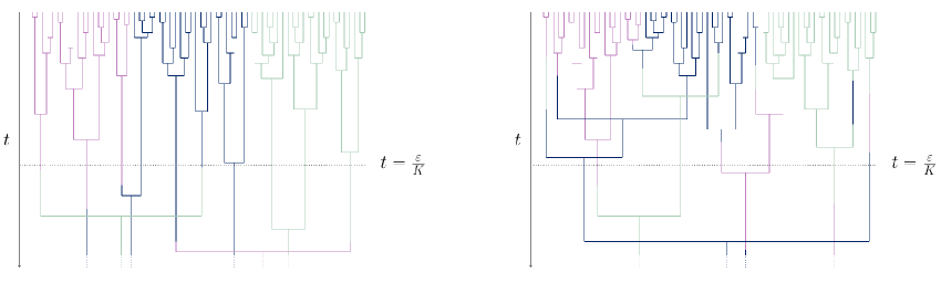
The proof of Proposition 5.1 builds on the following intuition (see Fig. 4). At small times, the coalescence rate is much higher than the migration rate. Therefore, we expect that, while coalescence reduces the number of blocks to , the impact of migration is of a smaller order and can be neglected. More precisely, we will see that in a typical block at colony the number of elements of colors different from is much smaller than the scaling factor .
To make this intuition precise, we will introduce two new measures and , the first accounting for the mono-chromatic part of the process and the second for the poly-chromatic part. To do this, we order the blocks in each colony according to their least element and denote by , , the number of elements of type in the -th block in colony ; we refer to as the internal coloring of the block. We then set
| (5.2) | ||||
| (5.3) |
Note that even if , we still have for
and hence
We will dedicate Subsections 5.2.1 and 5.2.2 respectively to the analysis of the monochromatic and the polychromatic parts in the previous expression.
5.2.1. Mono-chromatic part
The first thing to note here is that the total number of elements of color counted across all colonies remains constant, as migration simply moves elements from one colony to another. No elements change color, nor are they created or destroyed. So, if we only consider colony , we lose elements of color due to migration to other colonies, although it is possible that some of them might return (also due to migration).
The next result, loosely speaking, states that we can neglect the impact of migration at small times .
Lemma 5.2.
Let be defined as in Eq. (5.2). Then
Proof.
Recall that we start with singletons in colony , and note that
where denotes the number of elements of color that are not present in colony at time . It remains to show
To do this, we will construct a process that upper bounds ; the key ingredients are
-
(1)
Migrations of blocks to colony without any element of color do not affect . Thus, when constructing we can remove at time all singletons with a color different from and only keep the singletons of color .
-
(2)
When a block in colony with elements of color migrates, it adds to , but reduces the number of blocks in colony , and therefore the rate of migration out of colony . Thus, when constructing , at such a transition we will duplicate the block, keeping one copy in colony and the other contributing to . This way, when a block migrates back to colony , its elements will have already duplicates in colony , and hence can ignore that migration event. Note that in doing this, we are overcounting the number of elements of color out fo colony , because the same element may contribute several times to , but not to .
Having this in mind, we construct our upper-bound process as follows (see Fig. 5).
-
•
We set and start a (single-type) Kingman coalescent with rate with singletons.
-
•
At rate , with , per block of the Kingman coalescent, we count the number of elements within that block and increase by that amount the value of .
Let denote the rescaled empirical measure of the single-type Kingman coalescent described above. Then, for functions , the generator of is given as
with
Consider first the function defined via . Note that is constant in its second component, and that it is invariant under coalescence events. Thus,
| (5.4) |
Consider now the function defined via . Since is constant in its first component, we have . Moreover, we have
Since , using Dynkin’s formula and Eq. (5.4) yields
and therefore,
In particular
The result follows taking . ∎
5.2.2. Poly-chromatic part
The next result tells us that in colony the number of elements of a different color is much smaller than in .
Lemma 5.3.
Let be defined as in (5.3). Then
Proof.
A straightforward calculation yields
where and denotes the number of elements, with a color different than , present in colony at time . It remains to show
For this, note first that
where is defined in the proof of Lemma 5.2. Using this and the upper bound we obtained in the proof of Lemma 5.2, we get
The result follows taking . ∎
We conclude this section with the proof of Proposition 5.1.
Proof of Proposition 5.1.
Appendix A Uniqueness and stochastic representation for the critical sampling
Before diving into the proof of Theorem 2.8, let us prove the following result about the uniqueness of solutions to the discrete coagulation equation.
Proposition A.1.
Proof.
Assume that is a solution of (2.3) with initial condition (2.4). Define . A straightforward calculation shows that solves the system of equations
| (A.1) |
with initial condition . According to Picard-Lindelöf theorem, that initial value problem has at most solution. Since we have one solution, that solution is uniquely determined.
Second, let us now fix . Note that solves the system of non-linear odes
where is the solution of the system of equations (A.1) with initial condition . This is a finite dimensional system, and its solution is again uniquely determined by the initial condition, due to the Picard-Lindelöf theorem. The result follows as was arbitrarily chosen. ∎
Now we proceed with the proof of Theorem 2.8 and therefore assume that is the equilibrium probability measure, i.e.
Proof of Theorem 2.8.
Let be the solution of the discrete coagulation equation (2.3) under initial condition (2.4). For , define and
Hence,
For the first term we have
| (A.2) |
For the second term, recalling that solves (2.3), we find
| (A.3) |
Combining the previous identities yields after a tedious, but straightforward calculation
| (A.4) |
Since is assumed to be the equilibrium measure, the last term on the RHS vanishes, and we see that is the unique solution to the system of equations
| (A.5) |
with initial condition (uniqueness follows by standard results).
Let us now consider a continuous-time multi-type branching process such that, each particle of type
-
•
branches and dies at rate ,
-
•
makes a transition from to at rate .
It is straightforward to check that the function satisfies the system of equations (A.5) and the initial condition . Thus, by uniqueness of this initial value problem, we infer that
and the result follows. ∎
Remark A.2 (Stochastic representation beyond equilibrium).
Hence, assuming that (for example choosing sufficiently large), and proceeding as in the proof of Theorem (2.8), we deduce that
where is a multi-type branching process such that each particle of type
-
•
branches at rate ,
-
•
dies at rate ,
-
•
makes a transition from to at rate .
Acknowledgements
The authors would like to thank Sebastian Hummel for insightful discussions at an early stage of the project. Fernando Cordero and Sophia-Marie Mellis are funded by the Deutsche Forschungsgemeinschaft (DFG, German Research Foundation) — Project-ID 317210226 — SFB 1283.
References
- Aldous [1978] D. Aldous. Stopping times and tightness. Ann. Probab., 6:335–340, 1978. doi: 10.1214/aop/1176995579.
- Aldous [1999] D. J. Aldous. Deterministic and stochastic models for coalescence (aggregation and coagulation): a review of the mean-field theory for probabilists. Bernoulli, 5:3–48, 1999. doi: 10.2307/3318611.
- Bertoin and Le Gall [2006] J. Bertoin and J.-F. Le Gall. Stochastic flows associated to coalescent processes. III. Limit theorems. Illinois J. Math., 50:147–181, 2006.
- Billingsley [1999] P. Billingsley. Convergence of Probability Measures. Wiley, New York, 2nd edition, 1999. doi: 10.1002/9780470316962.
- Deaconu and Tanré [2000] M. Deaconu and E. Tanré. Smoluchowski’s coagulation equation: probabilistic interpretation of solutions for constant, additive and multiplicative kernels. Ann. Scuola Norm. Sup. Pisa Cl. Sci. (4), 29:549–579, 2000.
- Fournier and Méléard [2004] N. Fournier and S. Méléard. A microscopic probabilistic description of a locally regulated population and macroscopic approximations. Ann. Appl. Probab., 14:1880–1919, 2004.
- Joffe and Métivier [1986] A. Joffe and M. Métivier. Weak convergence of sequences of semimartingales with applications to multitype branching processes. Adv. in Appl. Probab., 18:20–65, 1986. doi: 10.2307/1427238.
- Johnston et al. [2023] S. G. G. Johnston, A. Kyprianou, and T. Rogers. Multitype -coalescents. Ann. Appl. Probab., 33:4210–4237, 2023. doi: 10.1214/22-aap1891.
- Kingman [1982] J. F. C. Kingman. The coalescent. Stochastic Process. Appl., 13:235–248, 1982. doi: 10.1016/0304-4149(82)90011-4.
- Lambert and Schertzer [2020] A. Lambert and E. Schertzer. Coagulation-transport equations and the nested coalescents. Probab. Theory Related Fields, 176:77–147, 2020. doi: 10.1007/s00440-019-00914-4.
- Notohara [1990] M. Notohara. The coalescent and the genealogical process in geographically structured population. J. Math. Biol., 29:59–75, 1990. doi: 10.1007/BF00173909.
- Roelly-Coppoletta [1986] S. Roelly-Coppoletta. A criterion of convergence of measure-valued processes: application to measure branching processes. Stoch. Int. J. Probab. Stoch. Process., 17:43–65, 1986.
- Tran [2008] V. C. Tran. Large population limit and time behaviour of a stochastic particle model describing an age-structured population. ESAIM Probab. Stat., 12:345–386, 2008.
- Tran [2014] V. C. Tran. Une ballade en forêts aléatoires. Technical report, 2014.