A Learning-Based Inexact ADMM for Solving Quadratic Programs

Abstract

Convex quadratic programs (QPs) constitute a fundamental computational primitive across diverse domains including financial optimization, control systems, and machine learning. The alternating direction method of multipliers (ADMM) has emerged as a preferred first-order approach due to its iteration efficiency – exemplified by the state-of-the-art OSQP solver. Machine learning-enhanced optimization algorithms have recently demonstrated significant success in speeding up the solving process. This work introduces a neural-accelerated ADMM variant that replaces exact subproblem solutions with learned approximations through a parameter-efficient Long Short-Term Memory (LSTM) network. We derive convergence guarantees within the inexact ADMM formalism, establishing that our learning-augmented method maintains primal-dual convergence while satisfying residual thresholds. Extensive experimental results demonstrate that our approach achieves superior solution accuracy compared to existing learning-based methods while delivering significant computational speedups of up to $7\times,28\times$, and $22\times$ over Gurobi, SCS, and OSQP, respectively. Furthermore, the proposed method outperforms other learning-to-optimize methods in terms of solution quality. Detailed performance analysis confirms near-perfect compliance with the theoretical assumptions, consequently ensuring algorithm convergence.

Keywords: quadratic programs, learning to optimize, inexact alternating direction method of multiplier, long short-term memory networks, self-supervised learning

1 Introduction

Quadratic Programs (QPs), as a fundamental class of constrained optimization problems, find widespread applications across diverse domains, ranging from finance and engineering to machine learning. In finance, a prominent example is portfolio optimization, where QPs are employed to allocate assets by optimizing the trade-off between expected returns and risk exposure (Boyd et al., 2013, Xiu et al., 2023). Control engineering, on the other hand, frequently relies on solving sequential QPs at each time step, necessitating extremely rapid computation to satisfy real-time control requirements (Garcia et al., 1989, Borrelli et al., 2017). Similarly, in machine learning, numerous unconstrained optimization problems—such as LASSO regression (Tibshirani, 1996), support vector machines (Cortes, 1995), and Huber regression (Huber and Ronchetti, 2011)—can be equivalently reformulated as QPs, as demonstrated in (Stellato et al., 2020). Given this extensive applicability, the development of efficient and accurate QP-solving algorithms remains a critical research pursuit.

Interior-point methods (IPMs) constitute a fundamental class of algorithms for solving QPs and serve as the computational backbone of leading commercial solvers including MOSEK (ApS, 2019) and Gurobi (Gurobi Optimization, 2023). As a second-order method, IPMs have gained widespread adoption for various nonlinear programs (Wächter and Biegler, 2006). In practice, modern implementation predominantly employs an infeasible path-following primal-dual approach, which initiates from potentially infeasible points and iteratively solves the perturbed KKT conditions via the Newton’s method, while enforcing centrality conditions via line search. These methods generate iterates that follow central paths, progressively reducing infeasibility while converging to optimal solutions. Each iteration requires solving a Newton system through matrix factorization, with computational complexity up to $\mathcal{O}(n^{3})$ for dense matrices. Consequently, despite exhibiting quadratic convergence rates, IPMs face significant challenges in scaling to large-scale or ill-conditioned problems. Furthermore, the central path trajectory inherently limits the effectiveness of warm-start strategies (John and Yıldırım, 2008), presenting additional computational bottlenecks for practical implementation.

First-order methods, which rely solely on gradient information, have emerged as powerful alternatives to second-order methods in large-scale optimization due to their computational efficiency. Notable examples include the primal-dual hybrid gradient (PDHG, He et al. (2014)) algorithm and the alternating direction method of multipliers (ADMM, Boyd et al. (2011)). Applegate et al. (2021) pioneered the application of PDHG to linear programs, achieving accuracy comparable to traditional solvers while demonstrating enhanced computational efficiency through matrix-free operations. Efficient parallelization is enabled by the algorithmic structure, allowing significant wall-clock time reduction through GPU acceleration. Building upon these advancements, Lu and Yang (2023) extended the PDHG framework to QPs, which attains linear convergence under mild regularity conditions while maintaining hardware-agnostic implementation across both GPU and CPU architectures. Mathematically equivalent to Douglas-Rachford splitting (Lions and Mercier, 1979), ADMM is particularly suitable for noise-prone environments where computationally efficient, near-optimal solutions are acceptable. The splitting conic solver (SCS, O’donoghue et al. (2016), O’Donoghue (2021)), a leading ADMM-based implementation, solves convex conic programs through careful dual variable tuning. While any QP can be reformulated as a conic program, such reformulation is often inefficient from a computational point of view. Our focus, the operator splitting quadratic programming (OSQP, Stellato et al. (2020)) solver, represents a specialized ADMM variant optimized for convex QPs through adaptive parameter updates that alleviates computational burden from expensive matrix factorization.

Recently, Learning to Optimize (L2O) has emerged as a transformative paradigm that integrates machine learning with numerical optimization to improve computational efficiency, demonstrating particular effectiveness for optimization problems with repetitive structural patterns. The foundational work of Gregor and LeCun (2010) proposed the learned iterative shrinkage thresholding algorithm, establishing the L2O approach by incorporating trainable parameters into optimization update steps and empirically demonstrating accelerated convergence through data-driven learning. Subsequent research has significantly expanded L2O methodologies across various domains, encompassing unconstrained optimization (Andrychowicz et al., 2016, Liu et al., 2023), linear optimization (Chen et al., 2022, Li et al., 2024), combinatorial optimization (Nair et al., 2020, Gasse et al., 2022), and constrained nonlinear programs (Donti et al., 2021, Liang et al., 2023, Gao et al., 2024). They demonstrate remarkable effectiveness when applied to problems with well-defined input distributions. Our investigation specifically targets the development of L2O techniques for convex QPs, a crucial subset within constrained optimization frameworks that merits particular attention.

Feasibility and optimality represent two core requirements in constrained L2O frameworks. While both supervised and self-supervised learning offer viable approaches, supervised methods critically depend on computationally expensive labeled datasets—a requirement that self-supervised approaches avoid. This significant advantage motivates us to focus on self-supervised learning methodologies. For equality constraints, completion techniques (Donti et al., 2021) generate full solutions through algebraic transformations or numerical procedures applied to network outputs (Kim et al., 2023, Liang et al., 2023, Li et al., 2023). Inequality constraints are typically addressed via post-processing operations, including gradient-based correction (Donti et al., 2021), Lagrangian dual variable ascent (Kim et al., 2023), homeomorphic projections (Liang et al., 2023), and gauge mappings from $\ell_{\infty}$-norm domains (Li et al., 2023). Another prevalent self-supervised learning strategy incorporates penalty functions into loss formulations to mitigate constraint violation (Donti et al., 2021, Park and Van Hentenryck, 2023, Liang et al., 2023). For example, the work of Park and Van Hentenryck (2023) proposed a co-training framework via an augmented Lagrangian method. While effective at reducing feasibility gaps, penalty methods require meticulous parameter tuning and lack feasibility guarantees. More importantly, most existing L2O works lack convergence guarantees. A notable exception is the work of Gao et al. (2024), which embedded LSTM-based approximations within inexact IPMs and demonstrated that learning-based optimization algorithms could produce optimal solutions when approximations meet acceptable tolerances.

Several pioneering works have explored the integration of L2O techniques with the ADMM. The seminal work by Sun et al. (2016) first demonstrated this synergy by unrolling ADMM iterations for compressive sensing applications, showing that parameterizing critical operations could significantly improve efficiency for unconstrained inverse problems. However, the systematic configuration of convergence-governing parameters in ADMM for convex QPs remains an open research challenge. Addressing this gap, Ichnowski et al. (2021) made substantial advances by developing a reinforcement learning framework to dynamically adapt penalty parameters in OSQP, achieving notable performance improvements through policy gradient optimization. Complementary approaches have explored warm-start strategies, exemplified by the hybrid architecture developed by Sambharya et al. (2023), which synergizes neural network-generated primal-dual initializations with fixed-iteration Douglas-Rachford splitting. These developments collectively highlight the inherent compatibility between ADMM and machine learning paradigms, maintaining theoretical convergence guarantees while exploiting learned priors for computational acceleration.

Although certain L2O algorithms possess theoretical convergence guarantees, a significant theory-practice gap persists in their practical implementation. For constrained optimization problems, this discrepancy manifests through substantial optimality gaps and measurable constraint violation in real-world applications. The L2O paradigm of obtaining approximate solutions represents a departure from exact methods, yet aligns with classical inexact optimization frameworks—where controlled approximations accelerate convergence while maintaining theoretical guarantees, as evidenced in Newton-type methods (Bellavia, 1998), IPMs (Eisenstat and Walker, 1994), and ADMM (Bai et al., 2025, Xie, 2018). Within ADMM specifically, inexact subproblem solutions have proven particularly effective: Xie (2018) established rigorous relative-error criteria for inexact resolution that enable more aggressive multiplier updates, while Bai et al. (2025) extended these principles to nonconvex problems under proper conditions. By ensuring neural network outputs comply with these established inexactness criteria, algorithmic convergence could be still maintained. As demonstrated by Gao et al. (2024), empirical adherence to residual bounds in IPMs allows learning-based methods to preserve theoretical guarantees. Hence, in this work, we introduce a novel LSTM-based framework for generating inexact solutions to ADMM subproblems, called “I-ADMM-LSTM”. The proposed architecture employs self-supervised learning on primal-dual residuals across fixed-length iteration windows, with convergence guaranteed when LSTM outputs satisfy inexact ADMM-derived primal-dual conditions. A refinement stage incorporating limited exact ADMM iterations (requiring only a single factorization) further enhances solution quality. The distinct contributions of our work can be summarized as follows:

• Learning-based ADMM. We present a novel neural architecture that seamlessly integrates traditional ADMM mechanics with deep learning. The framework employs a single LSTM cell to approximate ADMM subproblem solutions while maintaining consistency with update rules in OSQP. A carefully designed residual-driven loss function simultaneously minimizes primal and dual feasibility gaps, enabling stable convergence without requiring labeled training data.

• Theoretical Guarantee. By formulating our learned solver as an inexact ADMM variant, we establish verifiable conditions under which approximate subproblem solutions ensure convergence. This theoretical analysis connects approximation errors to algorithmic stability, providing quantifiable bounds on primal-dual residual decay throughout the optimization process.

• Computational Efficiency. Through extensive evaluation across multiple benchmark problems, our proposed approach achieves solutions with superior feasibility compared to state-of-the-art learning-based alternatives while delivering significant computational advantages—yielding up to $7\times$, $28\times$ and $22\times$ speed improvements over Gurobi, SCS, and OSQP, respectively. These results highlight the distinctive capability of our framework to maintain optimization rigor while achieving substantial computational gains.

The remainder of this paper is structured as follows. Section 2 presents the theoretical foundations of classical ADMM algorithms for convex QPs and derives convergence conditions for inexact ADMM variants. Section 3 introduces our novel learning-augmented ADMM framework, detailing its architecture and training methodology. The theoretical analysis regarding convergence properties of the proposed method appears in Section 4. Comprehensive numerical experiments on several benchmark problems, demonstrating the practical performance of our approach, are presented in Section 5. Finally, Section 6 provides concluding remarks that discuss limitations of the proposed method and identify promising directions for future research. For reproducibility and community benefit, our implementation is publicly available at https://github.com/NetSysOpt/I-ADMM-LSTM.

This paper employs the following mathematical conventions: The symbols $\mathbb{R}$, $\mathbb{R}^{n}$, and $\mathbb{R}^{n\times m}$ denote the sets of real numbers, $n$-dimensional real vectors, and $n\times m$ real matrices, respectively. The cone of $n\times n$ positive semidefinite matrices is represented by $\mathbb{S}^{n}_{+}$. We utilize $\mathbb{I}$ for the indicator function, with $I$ and $0$ designating the identity matrix and zero scalar/vector/matrix of appropriate dimensions. For symmetric matrices $A$ and $B$ having matching dimensions, the expressions $A\succ B$ and $A\succeq B$ indicate that $A-B$ is positive definite and positive semidefinite, respectively. The standard Euclidean norm on $\mathbb{R}^{n}$ is written as $\|\cdot\|$. When considering a positive semidefinite matrix $D\succeq 0$, we employ the weighted norm $\|x\|_{D}^{2}=x^{\top}Dx$. For an arbitrary matrix $A$, the notation $\text{Range}(A)$ refers to its range space, while $\kappa(A)$ represents its condition number. Finally, given a nonempty closed set $\mathcal{C}\subseteq\mathbb{R}^{n}$, the Euclidean distance from a point $x$ to $\mathcal{C}$ is expressed as $\text{dist}(x,\mathcal{C})=\inf_{z\in\mathcal{C}}\|x-z\|$.

2 ADMM for Convex QPs

This section introduces our convex QP formulation and derives an ADMM framework based on the widely-adopted OSQP solver. We subsequently develop an inexact ADMM variant that relaxes the solution accuracy requirements for subproblems, enabling effective incorporation of learning-based optimization approaches.

2.1 Problem Formulation

We consider the following convex QP:

$$\begin{array}[]{cl}\underset{x\in\mathbb{R}^{n}}{\operatorname{min}}&\frac{1}{2}x^{\top}Qx+p^{\top}x\\ \text{ s.t. }&l\leq Ax\leq u,\end{array}$$ (1)

where the decision variable $x\in\mathbb{R}^{n}$ is optimized over a quadratic objective function defined by a positive semidefinite matrix $Q\in\mathbb{S}^{n}_{+}$ and a linear term $p\in\mathbb{R}^{n}$. The linear constraints are specified by the matrix $A\in\mathbb{R}^{m\times n}$ with lower and upper bounds $l_{i}\in\mathbb{R}\cup\{-\infty\}$ and $u_{i}\in\mathbb{R}\cup\{+\infty\}$, respectively, for each constraint $i=1,\ldots,m$.

2.2 OSQP: An ADMM-Based Solver

This study focuses on OSQP, an ADMM-based first-order solver for convex QPs. Before detailing its iteration scheme, we first reformulate (1) through the introduction of auxiliary variables $z$ as follows:

$$\begin{array}[]{cl}\underset{x\in\mathbb{R}^{n}}{\operatorname{min}}&\frac{1}{2}x^{\top}Qx+p^{\top}x\\ \text{ s.t. }&Ax=z\\ &l\leq z\leq u.\end{array}$$ (2)

This reformulation enables efficient projection-based updates for $z$. Given initial primal variables $(x^{0},z^{0})\in\mathbb{R}^{n+m}$ and dual variables $y^{0}\in\mathbb{R}^{m}$, the ADMM iterations proceed as:

$$\left(x^{k+1},\tilde{z}^{k+1}\right) \leftarrow\underset{({x},\tilde{z}):A{x}=\tilde{z}}{\operatorname{argmin}}\;\frac{1}{2}{x}^{\top}Q{x}+p^{\top}{x}+\frac{\eta}{2}\|{x}-x^{k}\|_{2}^{2}+\frac{\rho}{2}\left\|\tilde{z}-z^{k}+\rho^{-1}y^{k}\right\|_{2}^{2},$$ (3)

$$z^{k+1} \leftarrow\Pi_{[l,u]}\left(\tilde{z}^{k+1}+\rho^{-1}y^{k}\right),$$ (4)

$$y^{k+1} \leftarrow y^{k}+\rho\left(\tilde{z}^{k+1}-z^{k+1}\right),$$ (5)

where $\eta,\rho>0$ denote penalty parameters, and $\Pi_{[l,u]}$ represents the projection operator onto $[l,u]$. The projection in step (4) ensures bound constraint satisfaction, while step (5) maintains complementary slackness through dual variable updates. This allows focusing exclusively on the convergence of primal and dual residuals:

$$r_{\text{primal}}\coloneqq Ax-z,\quad r_{\text{dual}}\coloneqq Qx+p+A^{\top}y,$$ (6)

with OSQP guaranteeing their asymptotic convergence to zero (Banjac et al., 2019). To address the equality-constrained quadratic subproblem (3), we focus on its optimality conditions:

$$\left[\begin{array}[]{ccc}Q+\eta I&&A^{\top}\\ &\rho I&-I\\ A&-I&\\ \end{array}\right]\left[\begin{array}[]{c}x\\ \tilde{z}\\ v\end{array}\right]=\left[\begin{array}[]{c}-p+\eta x^{k}\\ \rho z^{k}-y^{k}\\ 0\end{array}\right].$$ (7)

This linear system can be reduced to either: (i) a quasi-definite system solvable by direct methods (e.g., $L^{\top}DL$ factorization), or (ii) a positive definite system amenable to iterative methods (e.g., conjugate gradient). For direct solution methods, when both $\eta$ and $\rho$ remain fixed, only a single round of matrix factorization is required. In practical implementation, while $\eta$ is typically held constant, $\rho$ undergoes limited updates to balance primal-dual residuals - in such cases, only several rounds of matrix factorization are needed. This characteristic enables OSQP to achieve superior computational efficiency compared to second-order methods such as IPMs. Conversely, indirect methods are better suited for large-scale linear systems and can accommodate frequent updates of $\rho$.

2.3 Inexact ADMM Framework

Although the adaptive update rule for $\rho$ enhances computational efficiency of OSQP, solving subproblem (3) to exact optimality remains a computational bottleneck, particularly when dealing with large-scale matrices. To alleviate this issue, we propose an inexact ADMM approach that computes approximate solutions to (3). Since the $z$-update in (4) directly depends on $\tilde{z}$, our method naturally incorporates inexact solutions for $z$ as well. Following the inexact ADMM framework (Bai et al., 2025), we reformulate QPs of the form (1) as:

$$\begin{array}[]{cl}\underset{x\in\mathbb{R}^{n},z\in\mathbb{R}^{m}}{\operatorname{min}}&\frac{1}{2}x^{\top}Qx+p^{\top}x+\mathbb{I}_{l\leq z\leq u}(z)\\ \text{s.t.}&Ax=z,\\ \end{array}$$ (8)

where $\mathbb{I}_{l\leq z\leq u}(z)$ denotes the indicator function for bound constraints. The objective in (8) consists of a smooth quadratic component $f(x)\coloneqq\frac{1}{2}x^{\top}Qx+p^{\top}x$ and a nonsmooth proximal term $g(z)\coloneqq\mathbb{I}_{l\leq z\leq u}(z)$. For this two-block convex optimization structure, we employ ADMM with the following iterative steps:

$$x^{k+1} \leftarrow\underset{x\in\mathbb{R}^{n}}{\text{argmin}}\;\mathcal{L}_{\rho}(x,z^{k},y^{k})+\frac{\eta}{2}\|x-x^{k}\|^{2},$$ (9)

$$z^{k+1} \leftarrow\underset{z\in\mathbb{R}^{n}}{\text{argmin}}\;\mathcal{L}_{\rho}(x^{k+1},z,y^{k}),$$ (10)

$$y^{k+1} \leftarrow y^{k}+\rho\left(Ax^{k+1}-z^{k+1}\right),$$ (11)

where $\mathcal{L}(x,z,y)\coloneqq f(x)+g(z)+y^{\top}(Ax-z)$ and $\mathcal{L}_{\rho}(x,z,y)\coloneqq\mathcal{L}(x,z,y)+\frac{\rho}{2}\|Ax-z\|^{2}$ represent the Lagrangian and augmented Lagrangian functions for Problem (8), respectively.

Remark 1.

The steps in (9) – (11) generate iterates equivalent to those produced by (3) – (5). This equivalence holds because the optimality conditions (7) reduce to the linear system:

$$\left(Q+\eta I+\rho A^{T}A\right)x=\eta x^{k}-p+A^{T}\left(\rho z^{k}-y^{k}\right),$$ (12)

which exactly represents the optimality conditions for subproblem (9).

In numerous practical scenarios, obtaining exact solutions to subproblems (9) and (10) is could be computationally expensive, thus justifying the adoption of an inexact ADMM approach with approximation criteria. Our framework permits controlled inexact solutions for both $x^{k+1}$ and $z^{k+1}$ while preserving convergence guarantees. For the $x$-subproblem (9), the approximate solution $\tilde{x}^{k+1}$ must satisfy:

$$\mathcal{L}_{\rho}(\tilde{x}^{k+1},z^{k},y^{k})+\frac{\rho\beta_{x}}{2}\|\tilde{x}^{k+1}-x^{k}\|^{2}\leq\mathcal{L}_{\rho}(x^{k},z^{k},y^{k})$$ (13)

ensuring monotonic decrease of the augmented Lagrangian function, along with the gradient condition:

$$\|\xi_{x}^{k+1}\|\leq c_{x}\rho\|\tilde{x}^{k+1}-x^{k}\|,$$ (14)

for some $c_{x}>0$ and $\xi_{x}^{k+1}\coloneqq\nabla_{x}\mathcal{L}_{\rho}(\tilde{x}^{k+1},z^{k},y^{k})$. Similarly, the $z$-subproblem solution must obey:

$$\mathcal{L}_{\rho}(\tilde{x}^{k+1},z^{k+1},y^{k})+\frac{\rho\beta_{z}}{2}\|z^{k+1}-z^{k}\|^{2}\leq\mathcal{L}_{\rho}(\tilde{x}^{k+1},z^{k},y^{k}),$$ (15)

and the subgradient bound:

$$\|\xi_{z}^{k+1}\|\leq c_{z}\rho\left(\|z^{k+1}-z^{k}\|+\|\tilde{x}^{k+1}-x^{k}\|\right),$$ (16)

for $\xi_{z}^{k+1}\in\partial_{z}\mathcal{L}_{\rho}(\tilde{x}^{k+1},z^{k+1},y^{k})$ and $c_{z}>0$. The line search procedure employs a step size $\alpha^{k}\in(0,2)$ such that:

$$\mathcal{L}_{\rho}(x^{k+1},z^{k+1},y^{k+1})\leq\mathcal{L}_{\rho}(\tilde{x}^{k+1},z^{k+1},y^{k+1})-\delta\rho\|x^{k+1}-\tilde{x}^{k+1}\|^{2},$$ (17)

with $\delta\in(0,1)$. While analogous to the relaxation parameter of OSQP, $\alpha^{k}$ serves dual purposes of acceleration and stabilization.

Based on the preceding conditions (13) – (17), we derive an inexact ADMM algorithm (Algorithm 1) for solving (2). At iteration $k$, the algorithm computes approximate solutions $\tilde{x}^{k+1}$ and $z^{k+1}$ satisfying the specified conditions, followed by a dual variable update and line search procedure to maintain convergence guarantees. The iterative process terminates when the composite residual metric

$$R^{k+1}\coloneqq\|\tilde{x}^{k+1}-x^{k}\|+\|z^{k+1}-z^{k}\|+\|A\tilde{x}^{k+1}-z^{k+1}\|$$ (18)

falls below a predetermined tolerance threshold. As proven in Section 4, adherence to these conditions ensures global convergence to stationary points of the optimization problem.

Algorithm 1 Inexact ADMM for convex QPs

Input: Initial iterates $x^{0},z^{0},y^{0}$; parameters $\rho,\eta>0$, $\alpha\in(0,2)$

1:while $R^{k+1}>\epsilon_{\text{tol}}$ do

2:  Identify $\tilde{x}^{k+1}$ such that (13) and (14) satisfied

3:  Identify $z^{k+1}$ such that (15) and (16) satisfied

4:  $y^{k+1}\leftarrow y^{k}+\rho(\tilde{z}^{k+1}-z^{k+1})$

5:  Compute $x^{k+1}=\alpha^{k}\tilde{x}^{k+1}+(1-\alpha^{k})x^{k}$ via (17)

6:end while

3 Learning-based Inexact ADMM

Extending the inexact ADMM framework outlined in Section 2, we propose a learning-enhanced optimization methodology. The core innovation lies in replacing exact solutions to the ADMM subproblem (3) with learned approximations from LSTM networks, while preserving the ADMM iterative procedure. Figure 1 depicts the architecture of our Inexact ADMM with LSTM (denoted by I-ADMM-LSTM) framework, highlighting the integration of neural approximations with classical optimization components.

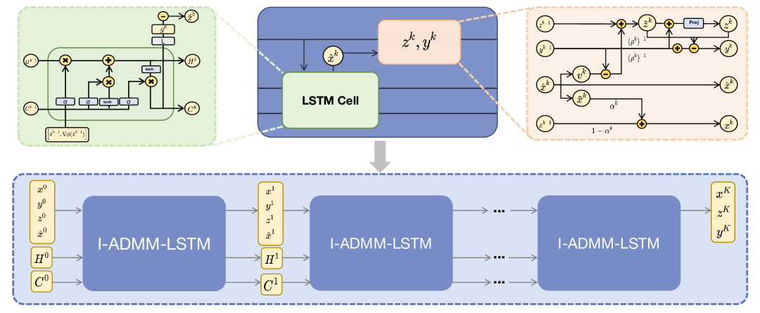
Figure 1: An illustration of the I-ADMM-LSTM approach.

3.1 I-ADMM-LSTM

To efficiently obtain inexact solutions for subproblem (3), we integrate learning-based techniques for solving its optimality conditions (7). To balance computational efficiency and numerical stability, we reformulate (7) into a condensed system:

$$\left[\begin{array}[]{cc}Q+\sigma I&A^{\top}\\ A&-\rho^{-1}I\end{array}\right]\left[\begin{array}[]{c}\tilde{x}^{k+1}\\ \nu^{k+1}\end{array}\right]=\left[\begin{array}[]{c}\sigma x^{k}-p\\ z^{k}-\rho^{-1}y^{k}\end{array}\right],$$ (19)

with $\tilde{z}^{k+1}$ being reconstructed as:

$$\tilde{z}^{k+1}=z^{k}+\rho^{-1}\left(\nu^{k+1}-y^{k}\right).$$ (20)

The system of equations (19) could be interpreted as a least-squares problem:

$$\min_{\hat{x}}\phi(\hat{x}):=\frac{1}{2}\left\|\hat{A}^{k}\hat{x}-\hat{b}^{k}\right\|^{2},$$ (21)

where $\hat{A}^{k}$ and $\hat{b}^{k}$ correspond to the coefficient matrix and right-hand side of (19), respectively. While such a linear system (19) can be further reduced in dimension, solving the resulting compact system would suffer from elevated condition numbers (Greif et al., 2014). The inclusion of $\eta$ ensures strong convexity of $\phi(\hat{x})$ in the least-squares formulation. A canonical approach for solving such problems involves first-order methods, particularly gradient-based algorithms, whose iterative structure makes them well-suited for solution trajectory approximation via L2O techniques (Andrychowicz et al., 2016, Gao et al., 2024).

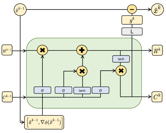
Figure 2: Coordinate-wise LSTM architecture for solving (21), where “L” represents the affine transformation layer.

To enhance computational efficiency, our framework incorporates a single coordinate-wise LSTM cell (Online Appendix A) to generate approximate solutions for (21), with its architecture detailed in Figure 2. The LSTM cell takes the previous output $\hat{x}^{k-1}$ and the gradient $\nabla\phi(\hat{x}^{k-1})$ as the input and outputs $\hat{x}^{k}$:

$$\hat{x}^{k}:=\operatorname{LSTM}_{\theta}\left(\left[\hat{x}^{k-1},\nabla\phi(\hat{x}^{k-1})\right]\right).$$ (22)

Our LSTM-based approach maintains parameter sharing across all iterations while seamlessly integrating with the primal-dual updates (4) and (5) from OSQP. Such a design could be considered as a novel recurrent neural network architecture tailored for convex QPs, which we refer to as I-ADMM-LSTM. Given initial primal-dual variables $\left(x^{0},z^{0},y^{0}\right)$ and LSTM inputs $x^{0}_{v},H^{0},C^{0}$, the algorithm iterates $K$ times to generate approximate solutions $\left(x^{K},z^{K},y^{K}\right)$, as outlined in Algorithm 2. The convergence of OSQP depends fundamentally on primal-dual residual reduction (6), which directly motivates us to choose the self-supervised loss function:

$$\min_{\theta}\frac{1}{|\mathcal{B}|}\sum_{B\in\mathcal{B}}\left(\frac{1}{K}\sum_{k=1}^{K}\left\|r_{\text{prim}}^{k}\right\|+\left\|r_{\text{dual}}^{k}\right\|\right)_{B},$$ (23)

where $\theta$ represents trainable network parameters and $\mathcal{B}$ comprises a dataset of identically distributed convex QPs. This formulation circumvents expensive label generation while ensuring convergence. To alleviate memory constraints, we implement truncated backpropagation through time (Liu et al., 2023), partitioning the $K$-iteration trajectory into $T$-length subsequences for gradient computation.

Algorithm 2 I-ADMM-LSTM for Convex QPs

Inputs: Initial values $x^{0},z^{0},y^{0},\hat{x}^{0},H^{0},C^{0}$, step size parameter $\eta>0$ and maximum iteration number $K$

Outputs: $x^{K},z^{K},y^{K}$

1:for $k\leftarrow 0$ to $K-1$ do

2:  $\hat{x}^{k+1}\leftarrow\operatorname{LSTM}_{\theta}\left(\left[\hat{x}^{k},\nabla\phi(\hat{x}^{k})\right]\right)$  

3:  $\tilde{x}^{k+1}\leftarrow\hat{x}^{k+1}[:n],v^{k+1}\leftarrow\hat{x}^{k+1}[n:]$ 

4:  $\tilde{z}^{k+1}\leftarrow z^{k}+({\rho^{k+1}})^{-1}(v^{k+1}-y^{k})$  

5:  $z^{k+1}\leftarrow\Pi_{[l,u]}\left(\tilde{z}^{k+1}+({\rho^{k+1}})^{-1}y^{k}\right)$  

6:  $y^{k+1}\leftarrow y^{k}+{\rho^{k+1}}\left(\tilde{z}^{k+1}-z^{k+1}\right)$  

7:  $x^{k+1}\leftarrow{\alpha^{k+1}}\tilde{x}^{k+1}+(1-{\alpha^{k+1}})x^{k}$ 

8:end for

3.2 Adaptive Parameters

Parameters $\rho,\eta$ and $\alpha$ in Algorithm 1 significantly influence the convergence rate, numerical stability, and primal-dual trade-offs within the optimization process. To enhance algorithmic adaptability, we propose a unified framework for dynamic parameter adaptation: the regularization parameter $\eta>0$, ensuring solution uniqueness in (3), is fixed as a small constant (e.g., $\eta=10^{-6}$) to preserve numerical stability. The relaxation parameter $\alpha^{k}\in(0,2)$ is parameterized via a sigmoid transformation

$$\alpha^{k}=2\cdot\sigma({\bar{\alpha}^{k}}),k=1,\cdots,K$$ (24)

where $\sigma(\cdot)$ denotes the sigmoid function and ${\bar{\alpha}^{k}}\in\mathbb{R}$ is a learnable scalar, eliminating heuristic line search while enforcing domain constraints. For the penalty parameter $\rho>0$, we prioritize active constraints by defining $\rho^{k}\coloneqq\operatorname{diag}\left(\rho^{k}_{1},\ldots,\rho^{k}_{m}\right)$, where each diagonal entry adapts as:

$$\rho^{k}_{i}\coloneqq\begin{cases}{\sigma({\bar{\rho}^{k}})}&l_{i}\neq u_{i}\,(\text{inactive}),\\ 10^{3}\cdot\sigma({\bar{\rho}^{k}})&l_{i}=u_{i}\,(\text{active}),\end{cases}$$ (25)

with ${\bar{\rho}^{k}}\in\mathbb{R}$ trainable. The sigmoid function ensures $\rho>0$ and mitigates gradient explosion. The self-supervised loss function, which minimizes primal and dual residuals (6), inherently balances primal-dual trade-offs through learned $\rho^{k}$ updates, aligning with principles in He et al. (2000). Crucially, unlike the shared LSTM parameters in Algorithm 1, $\alpha^{k}$ and $\rho^{k}$ are iteration-specific, enabling context-aware adjustments tailored to transient constraint activity. This design enhances adaptability across diverse problem geometries while maintaining numerical robustness, particularly in mixed active/inactive constraint regimes.

3.3 The Two-Stage Framework

To address the persistent challenge faced by learning-based methods in achieving sufficient proximity to optimal solutions while mitigating mild feasibility violations, we introduce a two-stage framework, termed I-ADMM-LSTM-FR (Feasibility-Restoration), designed to refine solution quality. The architecture of this approach is illustrated in Figure 3. The first stage employs I-ADMM-LSTM to generate approximate solutions via end-to-end neural optimization. This stage leverages learned optimization dynamics to achieve computational superiority over traditional solvers, albeit with mild feasibility violations. The second stage initializes with the primal-dual variables $(x^{K},y^{K},z^{K})$ and adaptive penalty parameter $\rho^{K}$ from Stage I. It executes a fixed number of exact ADMM iterations, resolving subproblem (3) via direct linear system solvers. Computational overhead is minimized through parameter freezing (fixing $\rho^{K}$ and disabling online tuning) and single matrix factorization reuse (leveraging precomputed $LU$ decompositions). For time-critical applications, the first stage alone suffices, while safety-critical domains benefit from the full I-ADMM-LSTM-FR pipeline.

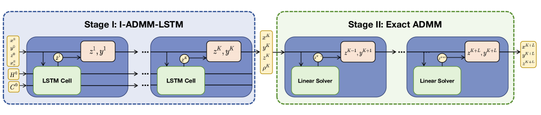
Figure 3: An illustration of the I-ADMM-LSTM-FR approach.

4 Convergence Analysis

In this section, we analyze the convergence of Algorithm 2 under the assumption that I-ADMM-LSTM satisfies conditions (13) – (17) outlined in Section 2.3. While empirical results demonstrate that the direct method in solving subproblem (3) enhances I-ADMM-LSTM for improved computational performance, our theoretical framework retains focus on the indirect method to preserve the equivalence between OSQP and the inexact ADMM framework. This alignment ensures rigorous adherence to convergence guarantees while maintaining methodological consistency.

The quadratic function $f(x)=\frac{1}{2}x^{\top}Qx+p^{\top}x$ possesses a Lipschitz-continuous gradient, satisfying:

$$\|\nabla f(x_{1})-\nabla f(x_{2})\|\leq\sigma_{Q}^{\text{max}}\|x_{1}-x_{2}\|$$ (26)

where $\sigma_{Q}^{\text{max}}>0$ denotes the largest eigenvalue of $Q$. We further impose:

Assumption 1.

For all $z\in\mathbb{R}^{m}$, $z\in\text{Range}(A)$.

Under this assumption, the dual variable update $y^{k+1}-y^{k}=\rho r^{k+1}$ lies in $\text{Range}(A)$, yielding:

$$\|y^{k+1}-y^{k}\|\leq\left(\sigma^{\text{min}}_{A^{\top}A}\right)^{{}^{-\frac{1}{2}}}\|A^{\top}\left(y^{k+1}-y^{k}\right)\|$$ (27)

where $\sigma_{A^{\top}A}^{\text{min}}$ is the smallest positive eigenvalue of $A^{\top}A$. To facilitate the analysis, we introduce the following notation:

$$\tilde{d}_{x}^{k}:=\tilde{x}^{k+1}-x^{k},\quad\hat{d}_{x}^{k}:=x^{k+1}-\tilde{x}^{k+1},\quad{d}_{z}^{k}:=z^{k+1}-z^{k}\quad\text{ and }\quad d_{y}^{k}:=y^{k+1}-y^{k}$$

We define the potential energy functions as

$$\tilde{E}^{k+1}:=\mathcal{L}_{\rho}\left(\tilde{x}^{k+1},z^{k+1},y^{k+1}\right)+\tilde{\Gamma}^{k},\quad\quad{E}^{k+1}:=\mathcal{L}_{\rho}\left(x^{k+1},z^{k+1},y^{k+1}\right)+\Gamma^{k}$$ (28)

where

$$\tilde{\Gamma}^{k}:=\frac{8\left(1+\tau\right)c^{2}_{x}\rho}{\sigma^{\text{min}}_{A^{\top}A}}\left\|\tilde{d}_{x}^{k}\right\|^{2}+8\left(1+\tau\right)\rho\kappa(A^{\top}A)\|d_{z}^{k}\|^{2},$$ (29)

$$\Gamma^{k}:=\tilde{\Gamma}^{k}+\frac{8\left(1+\tau\right)\left(\sigma_{Q}^{\text{max}}\right)^{2}}{\rho\sigma^{\text{min}}_{A^{\top}A}}\left\|\hat{{d}}_{x}^{k}\right\|^{2}$$ (30)

with $0<\tau<\delta<1$. Then, we can derive the following energy reduction proposition.

Proposition 1.

Suppose Assumption 1 holds, and Conditions (13), (14), (16) are satisfied. If the following conditions are satisfied:

$$\tilde{\mathcal{D}}_{x}:=\left[\frac{\beta_{x}(1-\tau)}{2(1+\tau)}-\frac{2\left(\frac{\sigma_{Q}^{\text{max}}}{\rho}+c_{x}\right)^{2}+8c_{x}^{2}}{\sigma^{\text{min}}_{A^{\top}A}}\right]I\succeq 0,$$ (31)

$$\hat{\mathcal{D}}_{x}:=\left[\frac{\delta-\tau}{1+\tau}-\frac{8\left(\frac{\sigma_{Q}^{\text{max}}}{\rho}\right)^{2}}{\sigma^{\text{min}}_{A^{\top}A}}\right]I\succeq 0,$$ (32)

$$\mathcal{D}_{z}:=\left[\frac{\beta_{z}(1-\tau)}{2(1+\tau)}-16\kappa(A^{\top}A)\right]I\succeq 0.$$ (33)

then for all $k\geq 1$, we have

$$E^{k+1}\leq E^{k}-\frac{\tau\rho\beta_{x}}{2}\left\|\tilde{d}_{x}^{k}\right\|^{2}-\frac{\tau\rho\beta_{z}}{2}\left\|d_{z}^{k}\right\|^{2}-\frac{\tau}{\rho}\left\|d_{y}^{k}\right\|^{2}-\tau\rho\|\hat{d}_{x}^{k}\|^{2},$$ (34)

$$\tilde{E}^{k+1}\leq\tilde{E}^{k}-\frac{\tau\rho\beta_{x}}{2}\left\|\tilde{d}_{x}^{k}\right\|^{2}-\frac{\tau\rho\beta_{z}}{2}\left\|d_{z}^{k}\right\|^{2}-\frac{\tau}{\rho}\left\|d_{y}^{k}\right\|^{2}-\tau\rho\|\hat{d}_{x}^{k-1}\|^{2}.$$ (35)

Readers are referred to Appendix C.2 for a detailed proof. Proposition 1 guarantees the monotonic decrease of the energy sequences $\{E^{k}\}_{k=1}^{\infty}$ and $\{\hat{E}^{k}\}_{k=1}^{\infty}$, forming the foundation for deriving global convergence of the proposed algorithm. A point $(x^{*},z^{*},y^{*})$ is stationary for Problem (8) if:

$$0=\nabla f\left(x^{*}\right)+A^{\top}y^{*},\quad 0\in\partial g\left(z^{*}\right)-y^{*}\quad\text{ and }\quad Ax^{*}=z^{*}.$$ (36)

Then, it is obvious that $(x^{k},z^{k},y^{k})$ is a stationary point if $R^{k}=0$. Hence, in the following convergence theorem, we assume $R^{k}\neq 0$ for all $k$.

Theorem 1.

Under Assumption 1 and Conditions (13) – (16), if $\tilde{E}^{k}$ is bounded below and (31) – (33) hold, there exists $F^{*}$ such that:

$$\lim_{k\rightarrow\infty}\mathcal{L}\left(x^{k},z^{k},y^{k}\right)=\lim_{k\rightarrow\infty}\mathcal{L}_{\rho}\left(x^{k},z^{k},y^{k}\right)=\lim_{k\rightarrow\infty}E^{k}=\lim_{k\rightarrow\infty}\tilde{E}^{k}=F^{*},$$ (37)

$$\lim_{k\rightarrow\infty}\operatorname{dist}\left(0,\partial\mathcal{L}\left(x^{k},z^{k},y^{k}\right)\right)=\lim_{k\rightarrow\infty}\operatorname{dist}\left(0,\partial\mathcal{L}_{\rho}\left(x^{k},z^{k},y^{k}\right)\right)=0.$$ (38)

Let $(x^{*},z^{*},y^{*})$ be a limit point of the sequence $\{(x^{k},z^{k},y^{k})\}$. Then $\{(x^{k},z^{k},y^{k})\}$ converges sublinearly to $(x^{*},z^{*},y^{*})$, and $(x^{*},z^{*},y^{*})$ is an optimal solution to (1).

Readers are referred to Appendix C.3 for a detailed proof. Theorem 1 states that Algorithm 2 achieves sublinear convergence to the optimal solution when mild assumptions are satisfied. Although the convergence rate appears slower in classical terms, I-ADMM-LSTM could achieve superior wall-clock performance by eliminating matrix factorization and hence enabling effective GPU parallelization.

5 Experiments

We present a systematic evaluation of the proposed I-ADMM-LSTM framework against classical optimization solvers and state-of-the-art L2O methods. The comparative analysis focuses on solving convex QPs across multiple benchmarks, quantifying the framework’s performance through objective value gaps, constraint satisfaction residuals, and runtime speedups.

5.1 Experimental Settings

5.1.1 Datasets.

The convex QPs used in this study include multiple datasets from Donti et al. (2021) and Stellato et al. (2020). For each dataset, we generated 1,000 samples, splitting them into training (940 samples), validation (10 samples), and test sets (50 samples). Additional dataset specifications are provided in Appendix D.

5.1.2 Baseline Algorithms.

In our experiments, we denote our proposed method as I-ADMM-LSTM and evaluate it against both classical optimization solvers and state-of-the-art L2O algorithms:

• Gurobi 10.0.3 (Gurobi Optimization, 2023): A state-of-the-art commercial solver employing advanced numerical techniques for linear, nonlinear, and mixed-integer programming.

• SCS (O’donoghue et al., 2016): An ADMM-based numerical solver for conic programming, which is employed through the CVX framework in this work to streamline implementation.

• OSQP (Stellato et al., 2020): An ADMM-based solver for convex QPs. For numerical precision assessment, we compare against two configurations: OSQP(1E-3) and OSQP(1E-4), with absolute/relative tolerances set to $10^{-3}$ and $10^{-4}$, respectively, and a maximum iteration limit of 20,000.

• DC3 (Donti et al., 2021): A constrained deep learning framework that ensures equality constraints via completion steps and enforces inequality constraints through correction mechanisms.

• PDL (Park and Van Hentenryck, 2023): A self-supervised L2O approach that co-trains primal and dual solution networks.

• LOOP-LC (Li et al., 2023): A neural operator leveraging gauge maps to generate feasible solutions for linearly constrained optimization problems.

5.1.3 Model Settings.

Our model is optimized using the Adam optimizer (Kingma, 2014). For I-ADMM-LSTM, we employ an early stopping criterion with a patience of 50 iterations, terminating training when no improvement in the objective value is observed for 50 consecutive epochs while maintaining both inequality and equality constraint violations below predetermined tolerance thresholds. The learning rate is fixed at $5\times 10^{-5}$ with a batch size of 2 per task. Task-specific hyperparameters for I-ADMM-LSTM are provided in Appendix D.

5.1.4 Configuration.

All experiments were executed on a computational platform equipped with an NVIDIA RTX A6000 GPU and an Intel Xeon 2.10GHz CPU, utilizing Python 3.10.0 and PyTorch 1.13.1.

5.2 Computational Results

We conduct a comprehensive evaluation of I-ADMM-LSTM (-FR) against baseline methods across multiple datasets, focusing on three critical performance metrics: solution optimality, constraint satisfaction, and computational efficiency. The experimental datasets are organized into two distinct groups, presented separately in Tables 1 and 2. Table 1 contains the “Convex QP (RHS)” dataset, following the experimental protocol established in Donti et al. (2021) and Gao et al. (2024), where only right-hand-side vectors undergo perturbation while all other parameters remain constant. Notably, we advance beyond previous work by scaling the problem size to 1,500 variables with 1,500 constraints, substantially exceeding the 200-variable limit employed in prior studies (Donti et al., 2021, Park and Van Hentenryck, 2023, Liang et al., 2023, Gao et al., 2024). Table 2 incorporates the “Convex QP (All)” dataset, where all parameters receive perturbations as implemented in Gao et al. (2024), along with additional synthetic datasets from (Stellato et al., 2020). While Table 1 includes comparisons with existing L2O baselines, these approaches are omitted from Table 2 due to the absence of representation learning approach for general convex QPs.

All methods were evaluated on 50 test instances, with metrics averaged to ensure statistical significance. The evaluation framework considers five key criteria: primal objective value (“Obj.”), mean inequality/equality constraint violation (“Mean ineq.” and “Mean eq.”), matrix factorization round count (“# Fac.”) - the dominant computational bottleneck for traditional solvers - iteration counts (“Ite.”), and total runtime (“Time (s)”). To ensure fair comparison, learning-based methods operated in single-instance mode (batch size=1) on GPU hardware.

Table 1 presents two problem scales for “Convex QP (RHS)”: (i) 1,000 variables with 500 inequality and 500 equality constraints, and (ii) 1,500 variables with 750 inequality and 750 equality constraints, as annotated in the “Instance” column. Traditional solvers Gurobi, SCS and OSQP each guarantee solution optimality through distinct approaches, with Gurobi achieving superior efficiency through its commercial-grade implementation - demonstrating $4\times$ and $3\times$ speed improvements over SCS and OSQP respectively on the 1,500-variable problems. While both SCS and OSQP utilize ADMM frameworks, SCS requires more iterations and incurs additional overhead from conic programming reformulations, leading to inferior performance compared to OSQP. The relaxed tolerance setting OSQP(1E-3) exhibits marginally larger optimality gaps and feasibility violations than OSQP(1E-4). Although relaxed tolerances reduce iteration counts, they provide limited reduction in matrix factorizations since $\rho$ updates occur only during substantial parameter variations, resulting in comparable total computation times. All L2O baseline algorithms returned solutions very quickly. However, learning-based approaches DC3 and PDL demonstrate significant constraint violations across both problem scales. While DC3 could ensure the satisfaction of equality constraints through “completion” techniques, its gradient-based “correction” fails to fully enforce inequality constraints. The end-to-end neural approach of PDL, lacking specialized feasibility mechanisms, shows more pronounced violations, particularly for inequality constraints. LOOP-LC maintains feasibility through combined completion and gauge projection but exhibits substantial optimality gaps. The proposed I-ADMM-LSTM eliminates matrix factorization through learned ADMM parameterization, achieving $6\times$, $21\times$, and $17\times$ speed improvements over Gurobi, SCS and OSQP respectively on 1,500-variable instances while maintaining optimality gaps within 2.4% of commercial solvers. The method demonstrates robust feasibility (mean violations $<0.017$) across both scales while surpassing Gurobi in computational efficiency. The enhanced I-ADMM-LSTM-FR variant incorporates a 20-iteration restoration phase (shown in the “Ite.” column) requiring one matrix factorization to completely eliminate constraint violations while preserving computational efficiency. Furthermore, this restoration yields measurable objective value improvements, driving solutions closer to optimality. In summary, I-ADMM-LSTM demonstrates faster computation than conventional solvers while outperforming other L2O baselines in both solution quality and feasibility across different problem scales.

Table 1: Comparative performance evaluation on “Convex QP (RHS)”.

Instance	Method	Obj.	Mean ineq. $\downarrow$	Mean eq. $\downarrow$	# Fac. $\downarrow$	Ite.	Time (s) $\downarrow$
Convex QP (RHS) (1000, 500, 500)	Gurobi	-152.701	0.000	0.000	-	14.3	0.824
	SCS	-152.701	0.000	0.000	-	75.0	2.285
	OSQP(1E-4)	-152.701	0.000	0.000	3.0	33.6	1.491
	OSQP(1E-3)	-152.705	0.002	0.001	3.0	28.3	1.456
	DC3	-112.894	0.175	0.000	-	-	0.056
	PDL	-131.568	0.002	0.555	-	-	0.025
	LOOP-LC	-108.525	0.000	0.000	-	-	0.042
	I-ADMM-LSTM	-147.334	0.002	0.017	0.0	100.0	0.217
	I-ADMM-LSTM-FR	-149.324	0.000	0.000	1.0	100.0 (20.0)	0.246
Convex QP (RHS) (1500, 750, 750)	Gurobi	-232.952	0.000	0.000	-	14.4	1.761
	SCS	-232.952	0.000	0.000	-	100.0	6.523
	OSQP(1E-4)	-232.952	0.000	0.000	3.0	38.6	5.140
	OSQP(1E-3)	-232.895	0.002	0.000	3.0	34.5	5.071
	DC3	-194.942	0.133	0.000	-	-	0.082
	PDL	-183.090	0.010	1.053	-	-	0.026
	LOOP-LC	0.094	0.000	0.000	-	-	0.026
	I-ADMM-LSTM	-227.257	0.002	0.015	0.0	150.0	0.303
	I-ADMM-LSTM-FR	-229.454	0.000	0.001	1.0	150.0 (20.0)	0.346

Similarly, we introduce additional datasets in Table 2, where all parameters are subject to perturbation, thus limiting our comparison to traditional methods. Consistent with the trends observed in Table 1, Gurobi demonstrates comparable computational efficiency to SCS and OSQP only on the “SVM” dataset, while exhibiting significantly superior performance across all the other test cases. More notably, on the newly introduced “Random QP”, “Equality QP”, and “SVM” datasets, I-ADMM-LSTM achieves remarkable solution quality even without any solution refinement, producing results that closely approximate optimal solutions both in terms of objective value and feasibility. The subsequent Stage II further enhances performance, as evidenced by I-ADMM-LSTM-FR matching the optimal objective values of Gurobi on the “Random QP” benchmark while delivering $3\times$ speed improvement.

Table 2: Comparative performance evaluation on synthetic datasets.

Instance	Method	Obj.	Mean ineq. $\downarrow$	Mean eq. $\downarrow$	# Fac. $\downarrow$	Ite.	Time (s) $\downarrow$
Convex QP (ALL) (1000, 500, 500)	Gurobi	-164.035	0.000	0.000	-	14.3	0.831
	SCS	-164.035	0.000	0.000	-	75.0	2.353
	OSQP(1E-4)	-164.035	0.000	0.000	3.1	35.9	1.558
	OSQP(1E-3)	-164.039	0.002	0.001	3.0	30.4	1.504
	I-ADMM-LSTM	-154.494	0.001	0.013	0.0	100.0	0.220
	I-ADMM-LSTM-FR	-158.822	0.000	0.000	1.0	100.0 (20.0)	0.258
Convex QP (ALL) (1500, 750, 750)	Gurobi	-251.073	0.000	0.000	-	14.8	1.701
	SCS	-251.073	0.000	0.000	-	100.0	6.666
	OSQP(1E-4)	-251.073	0.000	0.000	3.0	38.2	5.266
	OSQP(1E-3)	-251.077	0.002	0.000	3.0	33.5	5.081
	I-ADMM-LSTM	-232.944	0.002	0.022	0.0	100.0	0.232
	I-ADMM-LSTM-FR	-240.223	0.000	0.000	1.0	100.0 (20.0)	0.267
Random QP	Gurobi	-2.714	0.000	-	-	12.9	3.934
	SCS	-2.714	0.000	-	-	191.7	8.060
	OSQP(1E-4)	-2.714	0.000	-	3.0	93.9	10.765
	OSQP(1E-3)	-2.714	0.000	-	3.0	79.4	9.968
	I-ADMM-LSTM	-2.614	0.000	-	0.0	600.0	1.169
	I-ADMM-LSTM-FR	-2.716	0.000	-	1.0	600.0 (20.0)	1.215
Equality QP	Gurobi	249.722	-	0.000	-	5.3	0.794
	SCS	249.722	-	0.000	-	25.0	1.509
	OSQP(1E-4)	249.732	-	0.000	3.0	36.1	1.245
	OSQP(1E-3)	249.740	-	0.000	3.0	31.7	1.234
	I-ADMM-LSTM	249.713	-	0.000	0.0	400.0	0.846
	I-ADMM-LSTM-FR	250.501	-	0.000	1.0	400.0 (20.0)	1.001
SVM	Gurobi	547.880	0.000	-	-	6.8	0.236
	SCS	547.880	0.000	-	-	50.0	2.176
	OSQP(1E-4)	547.859	0.000	-	3.3	51.0	0.227
	OSQP(1E-3)	548.226	0.000	-	2.6	36.7	0.171
	I-ADMM-LSTM	545.800	0.000	-	0.0	50.0	0.134
	I-ADMM-LSTM-FR	545.711	0.000	-	1.0	50.0 (20.0)	0.171

5.3 Performance Analysis

5.3.1 Convergence Profiling.

We evaluate the baseline convergence characteristics of I-ADMM-LSTM (-FR) across diverse optimization benchmarks, focusing on four critical metrics: objective value trajectories, linear system solution residuals, and primal/dual residual dynamics (Figure 4). The results for three representative problem instances demonstrate consistent terminal convergence across all cases. To visualize, I-ADMM-LSTM is represented by blue lines, while the subsequent feasibility refinement process is depicted in green. All three datasets exhibit final convergence to optimal objective values, though initial fluctuations are observed for both “Equality_QP” and “SVM”, indicating some sensitivity to initialization choices. This observation suggests potential performance enhancements through more sophisticated initialization strategies. The solution accuracy for linear systems across all datasets evolves from relatively large initial residuals to significantly refined values, confirming the inexact nature of our algorithm. However, the concurrent convergence of primal-dual residuals to zero verifies that our inexact approach maintains theoretical convergence guarantees. While Stage II provides further improvement in objective values, occasional discontinuous jumps in primal-dual residuals suggest partial divergence between the exact ADMM and I-ADMM-LSTM solution paths. This behavior implies that the restoration stage may first adjust to its own convergence trajectory before proceeding with further optimization.

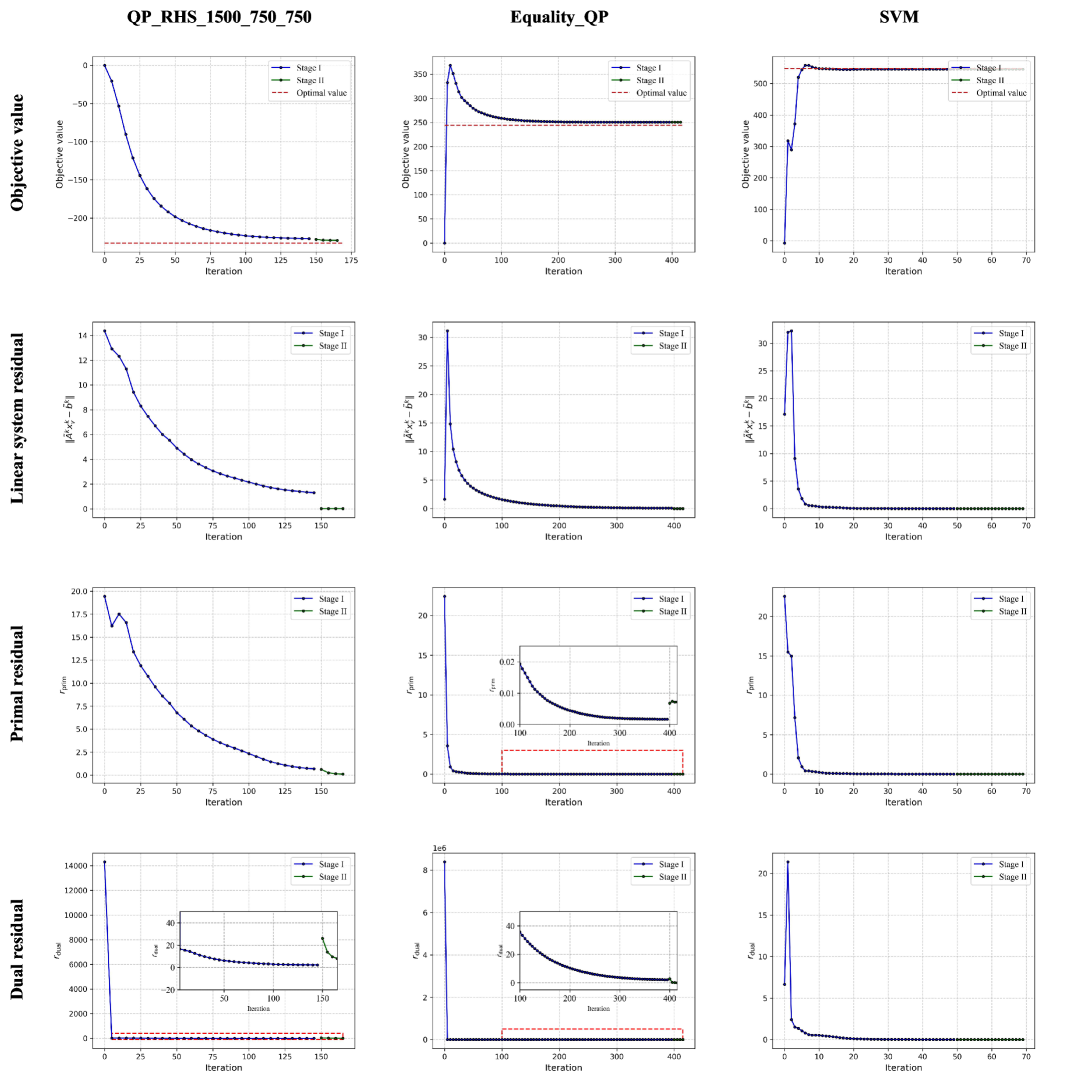
Figure 4: Convergence characteristics of I-ADMM-LSTM (-FR) across representative instances, illustrating objective value trajectories, linear system residuals, and primal/dual residual dynamics.

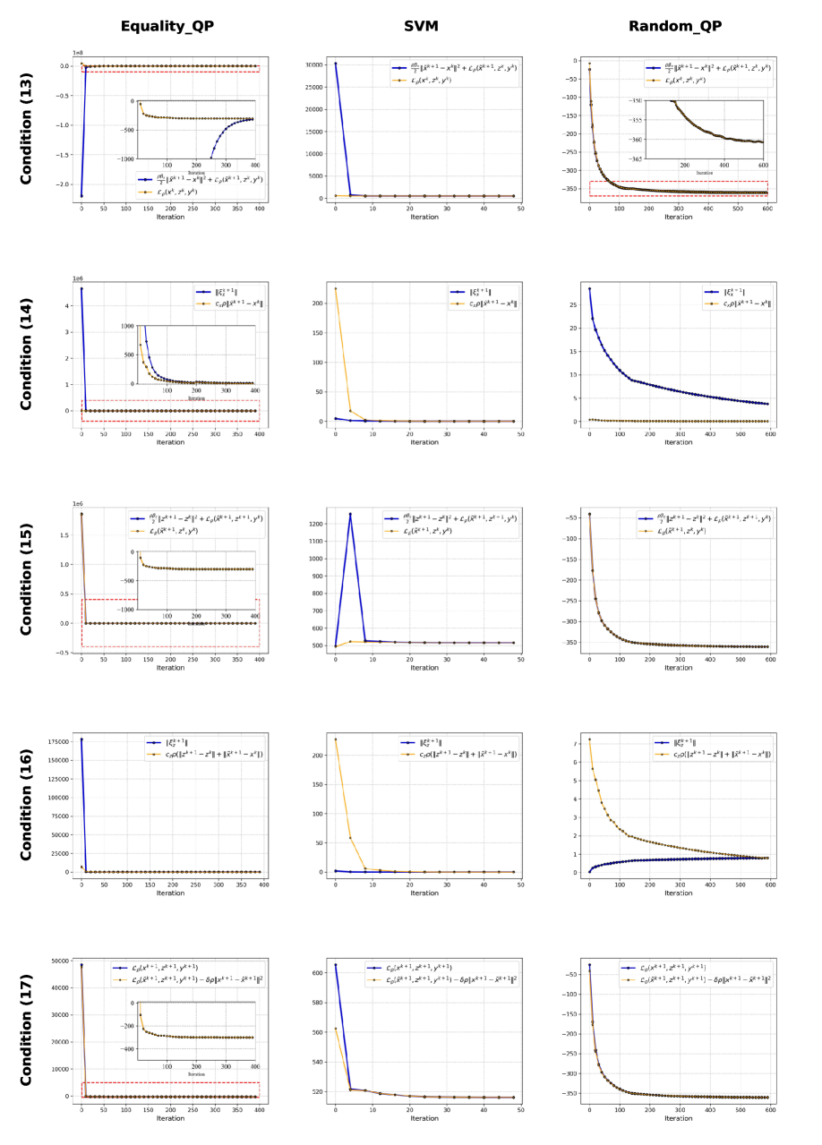
Figure 5: The satisfaction of conditions (13) – (17) across I-ADMM-LSTM iterations.

5.3.2 Empirical Validation.

Building upon the convergence framework established in Section 2.3, we empirically validate whether the proposed inexact ADMM conditions (13) – (17) hold in practical implementation. Following the experimental demonstrations of approximate optimality in Section 5.2, we assess whether conditions (13) – (17) hold by examining representative cases. Parameters are fixed as $c_{x}=1.0$, $c_{z}=1.0$ $\delta=0.9$ and $\tau=0.1$, with $\beta_{x}$ and $\beta_{z}$ derived via:

$$\beta_{x}=\frac{2(1+\tau)}{1-\tau}\left[\frac{2\left(\frac{\sigma_{Q}^{\text{max}}}{\rho}+1\right)^{2}+8}{\sigma^{\text{min}}_{A^{\top}A}}\right],\quad\beta_{z}=\frac{32(1+\tau)\kappa(A^{\top}A)}{1-\tau},$$ (39)

ensuring satisfaction of the bounding conditions (31) – (33). Figure 5 visualizes condition compliance across iterations, with blue/yellow curves denoting left/right-hand sides of inequalities.

Conditions (13) and (15) guarantee sufficient decrease of the augmented Lagrangian. The I-ADMM-LSTM framework generally maintains these conditions throughout optimization, with rare violations limited to initial iterations (typically $<10$ iterations for SVM-class problems). The gradient-based conditions (14) and (16) demand that $\tilde{x}^{k+1}$ and $z^{k}$ remain sufficiently close to stationary points of the augmented Lagrangian function, particularly in later iterations when primal-dual variable updates diminish and corresponding gradients should approach zero. While I-ADMM-LSTM satisfies these conditions well for “Equality QP” and “SVM” problems, significant violations occur for “Random QP” instances, consistent with Table 2 results showing remaining optimality gaps. The line search condition (17) requires adaptive step sizes $\alpha^{k}$ to further decrease the augmented Lagrangian function. In practice, the relatively stable values of the augmented Lagrangian function lead to near-equality satisfaction of condition (17). This empirical validation reveals a subtle yet critical gap between inexact computation and provable convergence, while simultaneously demonstrating that I-ADMM-LSTM approximately adheres to the convergence mechanisms of inexact ADMM frameworks.

6 Conclusions

In this study, we propose I-ADMM-LSTM, a learning-based inexact ADMM framework that approximates the ADMM subproblem solutions through a specialized LSTM network architecture. Our methodology demonstrates that machine-learned approximations via a single LSTM cell can maintain numerical convergence while accelerating computation. Extensive computational experiments on multiple convex QPs validate the effectiveness of I-ADMM-LSTM in generating high-quality primal-dual solutions. However, the current self-supervised learning framework inherently restricts its applicability to general nonlinear programs. Future research directions will focus on developing enhanced learning architectures capable of handling large-scale NLPs while preserving solution quality and convergence properties.

Appendix A Coordinate-wise LSTM

The coordinate-wise LSTM network addresses the unconstrained optimization problem $\min_{\hat{x}}\phi(\hat{x})$ through an iterative update scheme defined by the following operations:

$$X^{k} \leftarrow\left[\hat{x}^{k},\nabla\phi\left(\hat{x}^{k}\right)\right],$$ (40)

$$I^{k+1} \leftarrow{\sigma}\left(X^{k}W_{i}+H^{k}U_{i}+b_{i}\right),$$ (41)

$$F^{k+1} \leftarrow\sigma\left(X^{k}W_{f}+H^{k}U_{f}+b_{f}\right),$$ (42)

$$O^{k+1} \leftarrow\sigma\left(X^{k}W_{o}+H^{k}U_{o}+b_{o}\right),$$ (43)

$$\tilde{C}^{k+1} \leftarrow{\text{tanh}}\left(X^{k}W_{c}+H^{k}U_{c}+b_{c}\right),$$ (44)

$$C^{k+1} \leftarrow I^{k+1}\odot\tilde{C}^{k+1}+F^{k+1}\odot C^{k},$$ (45)

$$H^{k+1} \leftarrow O^{k+1}{\odot}\text{tanh}(C^{k+1}),$$ (46)

$$g^{k+1} \leftarrow H^{k+1}W_{g}+b_{g},$$ (47)

$$\hat{x}^{k+1} \leftarrow\hat{x}^{k}-g^{k+1},$$ (48)

where $H^{k}\in\mathbb{R}^{n\times h}$ (hidden state) and $C^{k}\in\mathbb{R}^{n\times h}$ (cell state) encode temporal dependencies, with $h$ denoting hidden units. Gating mechanisms regulate information flow: the input gate $I^{k}\in\mathbb{R}^{n\times h}$ governs feature integration into $C^{k}$, the forget gate $F^{k}\in\mathbb{R}^{n\times h}$ modulates retention of historical states $C^{k-1}$, and the output gate $O^{k}\in\mathbb{R}^{n\times h}$ controls state propagation through $H^{k}$. The update direction $g^{k}\in\mathbb{R}^{n}$, derived via $g^{k}=H^{k}W_{g}+b_{g}$, drives iterative parameter refinement. Trainable parameters include input weights $W_{i},W_{f},W_{o},W_{c}\in\mathbb{R}^{2\times h}$, recurrent weights $U_{i},U_{f},U_{o},U_{c}\in\mathbb{R}^{h\times h}$, output weights $W_{g}\in\mathbb{R}^{h\times 1}$, and biases $b_{i},b_{f},b_{o},b_{c}\in\mathbb{R}^{h}$, $b_{g}\in\mathbb{R}$. The operators $\sigma$, $\tanh$, and $\odot$ denote the sigmoid activation, hyperbolic tangent, and Hadamard product, respectively.

Appendix B Preconditioning

Preconditioning serves as a heuristic strategy to mitigate numerical instabilities in ill-conditioned optimization problems. Our framework adopts an efficient preconditioning method adapted from Stellato et al. (2020), designed to improve numerical conditioning while preserving computational tractability. A key advantage of this approach is its inherent parallelizability across optimization instances, critical for L2O pipelines requiring batch processing. Consider the symmetric matrix $M\in\mathbb{S}^{n+m}$, defined as:

$$M\coloneqq\left[\begin{array}[]{cc}P&A^{T}\\ A&0\end{array}\right].$$ (49)

We employ symmetric matrix equilibration through computation of a diagonal matrix $S\in\mathbb{S}_{++}^{n+m}$ to reduce the condition number of $SMS$. The matrix $S$ admits the diagonal representation:

$$S\coloneqq\begin{bmatrix}D&0\\ 0&E\end{bmatrix},$$ (50)

where $D\in\mathbb{S}_{++}^{n\times n}$ and $E\in\mathbb{S}_{++}^{m\times m}$ are diagonal matrices. To constrain dual variable magnitudes, a scaling coefficient $c>0$ is incorporated into the objective function. This preconditioning operation transforms the original QP problem (2) into a normalized form:

$$\begin{array}[]{ll}\underset{\bar{x}\in\mathbb{R}^{n}}{\min}&\frac{1}{2}\bar{x}^{\top}\bar{Q}\bar{x}+\bar{p}^{\top}\bar{x}\\ \text{ s.t. }&\bar{A}\bar{x}=z\\ &\bar{l}\leq z\leq\bar{u},\end{array}$$ (51)

where $\bar{x}=D^{-1}x$, $\bar{P}=cDQD$, $\bar{p}=cDp$, $\bar{A}=EAD$, $\bar{l}=El$ and $\bar{u}=Eu$. To find an $S$, we employ a modified Ruiz equilibration algorithm (Algorithm 3) from Stellato et al. (2020). This process enhances numerical stability while preserving problem sparsity.

Algorithm 3 Modified Ruiz equilibration

Inputs: Initial values $c^{0}=1,S^{0}=I,\delta^{0}=0,\bar{Q}^{0}=Q,\bar{p}^{0}=p,\bar{A}^{0}=A,\bar{l}^{0}=l,\bar{u}^{0}=u$ and Maximum number of iteration $K$

Outputs: $S^{K},c^{K}$

1:for $k\leftarrow 1$ to $K$ do

2:  for $i\leftarrow 1$ to $n+m$ do

3:   $\delta_{i}^{k}\leftarrow 1/\sqrt{\left\|M_{i}\right\|_{\infty}}$ 

4:  end for

5:  $\bar{Q}^{k},\bar{p}^{k},\bar{A}^{k},\bar{l}^{k},\bar{u}^{k}\leftarrow$ Scale $\bar{Q}^{k-1},\bar{p}^{k-1},\bar{A}^{k-1},\bar{l}^{k-1},\bar{u}^{k-1}$ using $\operatorname{diag}(\delta^{k})$  

6:  $\gamma^{k}\leftarrow 1/\max\left\{\operatorname{mean}\left(\left\|\bar{Q}_{i}^{k}\right\|_{\infty}\right),\|\bar{p}^{k}\|_{\infty}\right\}$ 

7:  $\bar{Q}^{k}\leftarrow\gamma^{k}\bar{Q}^{k},\bar{p}^{k}\leftarrow\gamma^{k}\bar{p}^{k}$ 

8:  $S^{k}\leftarrow\operatorname{diag}(\delta^{k})S^{k-1},c^{k}\leftarrow\gamma^{k}c^{k-1}$ 

9:end for

Appendix C Proofs

Prior to presenting the proof of Proposition 1, we first establish the following lemma:

Lemma 1.

Under Assumption 1 and Condition (14), the following inequality holds for all $k\geq 1$:

$$\begin{array}[]{cl}\|A^{\top}d_{y}^{k}\|^{2}\leq&2\left(\sigma_{Q}^{\text{max}}+c_{x}\rho\right)^{2}\|\tilde{d}_{x}^{k}\|^{2}+8\left(\sigma_{Q}^{\text{max}}\right)^{2}\|\hat{d}_{x}^{k-1}\|^{2}\\ &+8c_{x}^{2}\rho^{2}\|\tilde{d}_{x}^{k-1}\|^{2}+8\rho^{2}\sigma_{A^{\top}A}^{\text{max}}\left(\|d_{z}^{k}\|^{2}+\|d_{z}^{k-1}\|^{2}\right)\end{array}$$ (52)

C.1 Proof of Lemma 1

Beginning with the definition of the gradient $\xi_{x}^{k+1}=\nabla_{x}\mathcal{L}_{\beta}\left(\tilde{x}^{k+1},z^{k},y^{k}\right)$, we have

$$\begin{array}[]{cl}\xi_{x}^{k+1}&=\nabla f\left(\tilde{x}^{k+1}\right)+A^{\top}y^{k}+\rho A^{\top}\left(A\tilde{x}^{k+1}-z^{k}\right)\\ &=\nabla f\left(\tilde{x}^{k+1}\right)+A^{\top}y^{k}+\rho A^{\top}\left(A\tilde{x}^{k+1}-z^{k+1}+z^{k+1}-z^{k}\right)\\ &=\nabla f\left(\tilde{x}^{k+1}\right)+A^{\top}y^{k}+\rho A^{\top}\left(\tilde{r}^{k+1}+d_{z}^{k+1}\right)\\ \end{array}$$ (53)

where $\tilde{r}^{k+1}=A\tilde{x}^{k+1}-z^{k+1}$. Hence, we have

$$A^{\top}y^{k}=\xi_{x}^{k+1}-\nabla f\left(\tilde{x}^{k+1}\right)-\rho A^{\top}\tilde{r}^{k+1}-\rho A^{\top}d_{z}^{k}$$ (54)

Substituting the dual update $y^{k+1}=y^{k}+\rho\tilde{r}^{k+1}$ into (54) produces:

$$A^{\top}y^{k+1}=\xi_{x}^{k+1}-\nabla f\left(\tilde{x}^{k+1}\right)-\rho A^{\top}d_{z}^{k}$$ (55)

Letting $d_{y}^{k}=y^{k+1}-y^{k}$, we derive the equation:

$$A^{\top}d^{k}_{y}=\xi_{x}^{k+1}-\xi_{x}^{k}+\nabla f\left(\tilde{x}^{k}\right)-\nabla f\left(\tilde{x}^{k+1}\right)+\rho A^{\top}\left(d^{k-1}_{z}-d^{k}_{z}\right)$$ (56)

Squaring both sides and applying the Cauchy-Schwarz inequality:

$$\left\|A^{\top}d_{y}^{k}\right\|^{2} =\|\nabla f\left(\tilde{x}^{k}\right)-\nabla f\left(\tilde{x}^{k+1}\right)+\xi_{x}^{k+1}-\xi_{x}^{k}+\rho A^{\top}\left(d^{k-1}_{z}-d^{k}_{z}\right)\|^{2}$$ (57)

$$\leq\left[\sigma_{Q}^{\text{max}}\|\tilde{d}_{x}^{k}+\hat{d}_{x}^{k-1}\|+c_{x}\rho\left(\|\tilde{d}_{x}^{k}\|+\|\tilde{d}_{x}^{k-1}\|\right)+\rho\left(\|A^{\top}d_{z}^{k}\|+\|A^{\top}d_{z}^{k-1}\|\right)\right]^{2}$$

$$\leq\left[\left(\sigma_{Q}^{\text{max}}+c_{x}\rho\right)\|\tilde{d}_{x}^{k}\|+\sigma_{Q}^{\text{max}}\|\hat{d}_{x}^{k-1}\|+c_{x}\rho\|\tilde{d}_{x}^{k-1}\|+\rho\left(\|A^{\top}d_{z}^{k}\|+\|A^{\top}d_{z}^{k-1}\|\right)\right]^{2}$$

$$\leq 2\left(\sigma_{Q}^{\text{max}}+c_{x}\rho\right)^{2}\|\tilde{d}_{x}^{k}\|^{2}+8\left(\sigma_{Q}^{\text{max}}\right)^{2}\|\hat{d}_{x}^{k-1}\|^{2}+8c_{x}^{2}\rho^{2}\|\tilde{d}_{x}^{k-1}\|^{2}+8\rho^{2}\sigma_{A^{\top}A}^{\text{max}}\left(\|d_{z}^{k}\|^{2}+\|d_{z}^{k-1}\|^{2}\right)$$

C.2 Proof of Proposition 1

Building upon Lemma 1, we establish the proof of Proposition 1. Beginning with conditions (13), (15), and the dual residual bound (27), we decompose the Lagrangian difference:

$$\mathcal{L}_{\rho}\left(\tilde{x}^{k+1},z^{k+1},y^{k+1}\right)-\mathcal{L}_{\rho}\left(x^{k},z^{k},y^{k}\right)$$ (58)

$$= \mathcal{L}_{\rho}\left(\tilde{x}^{k+1},z^{k+1},y^{k+1}\right)-\mathcal{L}_{\rho}\left(\tilde{x}^{k+1},z^{k+1},y^{k}\right)+\mathcal{L}_{\rho}\left(\tilde{x}^{k+1},z^{k+1},y^{k}\right)$$

$$-\mathcal{L}_{\rho}\left(\tilde{x}^{k+1},z^{k},y^{k}\right)+\mathcal{L}_{\rho}\left(\tilde{x}^{k+1},z^{k},y^{k}\right)-\mathcal{L}_{\rho}\left(x^{k},z^{k},y^{k}\right)$$

$$\leq \frac{1+\tau}{\rho}\left\|d_{y}^{k}\right\|^{2}-\frac{\rho\beta_{z}}{2}\left\|d_{z}^{k}\right\|^{2}-\frac{\rho\beta_{x}}{2}\left\|\tilde{d}_{x}^{k}\right\|^{2}-\frac{\tau}{\rho}\left\|d_{y}^{k}\right\|^{2}$$

$$\leq \frac{1+\tau}{\rho\sigma^{\text{min}}_{A^{\top}A}}\left\|A^{\top}d_{y}^{k}\right\|^{2}-\frac{\rho\beta_{z}}{2}\left\|d_{z}^{k}\right\|^{2}-\frac{\rho\beta_{x}}{2}\left\|\tilde{d}_{x}^{k}\right\|^{2}-\frac{\tau}{\rho}\left\|d_{y}^{k}\right\|^{2}.$$

In addition, by (52), we obtain

$$\frac{1+\tau}{\rho\sigma^{\text{min}}_{A^{\top}A}}\left\|A^{\top}d_{y}^{k}\right\|^{2}$$ (59)

$$\leq \frac{1+\tau}{\rho\sigma^{\text{min}}_{A^{\top}A}}\left[2\left(\sigma_{Q}^{\text{max}}+c_{x}\rho\right)^{2}\|\tilde{d}_{x}^{k}\|^{2}+8\left(\sigma_{Q}^{\text{max}}\right)^{2}\|\hat{d}_{x}^{k-1}\|^{2}+8c_{x}^{2}\rho^{2}\|\tilde{d}_{x}^{k-1}\|^{2}+8\rho^{2}\sigma_{A^{\top}A}^{\text{max}}\left(\|d_{z}^{k}\|^{2}+\|d_{z}^{k-1}\|^{2}\right)\right].$$

Plugging (59) into (58), by (17) and , yields:

$$\mathcal{L}_{\rho}\left(x^{k+1},z^{k+1},y^{k+1}\right)-\mathcal{L}_{\rho}\left(x^{k},z^{k},y^{k}\right)$$ (60)

$$\leq \mathcal{L}_{\rho}\left(\tilde{x}^{k+1},z^{k+1},y^{k+1}\right)-\mathcal{L}_{\rho}\left(x^{k},z^{k},y^{k}\right)-\delta\rho\|x^{k+1}-\tilde{x}^{k+1}\|^{2}$$

$$\leq \frac{1+\tau}{\rho\sigma^{\text{min}}_{A^{\top}A}}\left[2\left(\sigma_{Q}^{\text{max}}+c_{x}\rho\right)^{2}\|\tilde{d}_{x}^{k}\|^{2}+8\left(\sigma_{Q}^{\text{max}}\right)^{2}\|\hat{d}_{x}^{k-1}\|^{2}+8c_{x}^{2}\rho^{2}\|\tilde{d}_{x}^{k-1}\|^{2}+8\rho^{2}\sigma_{A^{\top}A}^{\text{max}}\left(\|d_{z}^{k}\|^{2}+\|d_{z}^{k-1}\|^{2}\right)\right]$$

$$-\frac{\rho\beta_{z}}{2}\left\|d_{z}^{k}\right\|^{2}-\frac{\rho\beta_{x}}{2}\left\|\tilde{d}_{x}^{k}\right\|^{2}-\frac{\tau}{\rho}\left\|d_{y}^{k}\right\|^{2}-\delta\rho\|\hat{d}_{x}^{k}\|^{2}$$

$$= \frac{8\left(1+\tau\right)c^{2}_{x}\rho}{\sigma^{\text{min}}_{A^{\top}A}}\left(\left\|\tilde{d}_{x}^{k-1}\right\|^{2}-\left\|\tilde{{d}}_{x}^{k}\right\|^{2}\right)+\frac{8\left(1+\tau\right)\left(\sigma_{Q}^{\text{max}}\right)^{2}}{\rho\sigma^{\text{min}}_{A^{\top}A}}\left(\left\|\hat{d}_{x}^{k-1}\right\|^{2}-\left\|\hat{{d}}_{x}^{k}\right\|^{2}\right)+\frac{8\left(1+\tau\right)\rho\sigma^{\text{max}}_{A^{\top}A}}{\sigma^{\text{min}}_{A^{\top}A}}\left(\|d_{z}^{k-1}\|^{2}-\|d_{z}^{k}\|^{2}\right)$$

$$-\frac{\rho\beta_{z}}{2}\left\|d_{z}^{k}\right\|^{2}-\frac{\rho\beta_{x}}{2}\left\|\tilde{d}_{x}^{k}\right\|^{2}-\frac{\tau}{\rho}\left\|d_{y}^{k}\right\|^{2}-\delta\rho\|\hat{d}_{x}^{k}\|^{2}$$

$$+\frac{\left(1+\tau\right)\rho\left[2\left(\frac{\sigma_{Q}^{\text{max}}}{\rho}+c_{x}\right)^{2}+8c_{x}^{2}\right]}{\sigma^{\text{min}}_{A^{\top}A}}\|\tilde{d}^{k}\|^{2}+\frac{8\left(1+\tau\right)\left(\sigma_{Q}^{\text{max}}\right)^{2}}{\rho\sigma^{\text{min}}_{A^{\top}A}}\|\hat{d}^{k}_{x}\|^{2}+\frac{16\left(1+\tau\right)\rho\sigma^{\text{max}}_{A^{\top}A}}{\sigma^{\text{min}}_{A^{\top}A}}\|d_{z}^{k}\|^{2}$$

$$= \frac{8\left(1+\tau\right)c^{2}_{x}\rho}{\sigma^{\text{min}}_{A^{\top}A}}\left(\left\|\tilde{d}_{x}^{k-1}\right\|^{2}-\left\|\tilde{{d}}_{x}^{k}\right\|^{2}\right)+\frac{8\left(1+\tau\right)\left(\sigma_{Q}^{\text{max}}\right)^{2}}{\rho\sigma^{\text{min}}_{A^{\top}A}}\left(\left\|\hat{d}_{x}^{k-1}\right\|^{2}-\left\|\hat{{d}}_{x}^{k}\right\|^{2}\right)+\frac{8\left(1+\tau\right)\rho\sigma^{\text{max}}_{A^{\top}A}}{\sigma^{\text{min}}_{A^{\top}A}}\left(\|d_{z}^{k-1}\|^{2}-\|d_{z}^{k}\|^{2}\right)$$

$$-\frac{\tau\rho\beta_{x}}{2}\left\|\tilde{d}_{x}^{k}\right\|^{2}-\tau\rho\|\hat{d}_{x}^{k}\|^{2}-\frac{\tau\rho\beta_{z}}{2}\left\|d_{z}^{k}\right\|^{2}-\frac{\tau}{\rho}\left\|d_{y}^{k}\right\|^{2}$$

$$-\left(1+\tau\right)\rho\left(\|\tilde{d}^{k}_{x}\|^{2}_{\tilde{\mathcal{D}}_{x}}+\|\hat{d}_{x}^{k}\|^{2}_{\hat{\mathcal{D}}_{x}}+\|d_{z}^{k}\|^{2}_{\mathcal{D}_{z}}\right)$$

$$\leq \frac{8\left(1+\tau\right)c^{2}_{x}\rho}{\sigma^{\text{min}}_{A^{\top}A}}\left(\left\|\tilde{d}_{x}^{k-1}\right\|^{2}-\left\|\tilde{{d}}_{x}^{k}\right\|^{2}\right)+\frac{8\left(1+\tau\right)\left(\sigma_{Q}^{\text{max}}\right)^{2}}{\rho\sigma^{\text{min}}_{A^{\top}A}}\left(\left\|\hat{d}_{x}^{k-1}\right\|^{2}-\left\|\hat{{d}}_{x}^{k}\right\|^{2}\right)+8\left(1+\tau\right)\rho\kappa(A^{\top}A)\left(\|d_{z}^{k-1}\|^{2}-\|d_{z}^{k}\|^{2}\right)$$

$$-\frac{\tau\rho\beta_{x}}{2}\left\|\tilde{d}_{x}^{k}\right\|^{2}-\tau\rho\|\hat{d}_{x}^{k}\|^{2}-\frac{\tau\rho\beta_{z}}{2}\left\|d_{z}^{k}\right\|^{2}-\frac{\tau}{\rho}\left\|d_{y}^{k}\right\|^{2},$$

where $0<\tau<\delta<1$, $\kappa(A^{\top}A)$ denotes the condition number of $A^{\top}A$, $\tilde{\mathcal{D}}_{x}\succeq 0$, $\hat{\mathcal{D}}_{x}\succeq 0$ and $\mathcal{D}_{z}\succeq 0$ are defined in (31), (32) and (33), respectively. Then, (34) follows from (60) and the definition of $E^{k+1}$ in (28). Similarly, by (17) and $\hat{d}^{k}_{x}=x^{k+1}-\tilde{x}^{k+1}$, we have

$$\begin{array}[]{rl}\mathcal{L}_{\rho}(\tilde{x}^{k+1},z^{k+1},y^{k+1})-\mathcal{L}_{\rho}(\tilde{x}^{k},z^{k},y^{k})\leq&\mathcal{L}_{\rho}(\tilde{x}^{k+1},z^{k+1},y^{k+1})-\mathcal{L}_{\rho}(x^{k},z^{k},y^{k})-\delta\rho\|x^{k}-\tilde{x}^{k}\|^{2}\\ =&\mathcal{L}_{\rho}(\tilde{x}^{k+1},z^{k+1},y^{k+1})-\mathcal{L}_{\rho}(x^{k},z^{k},y^{k})-\delta\rho\|\tilde{d}^{k-1}_{x}\|^{2}\end{array}$$ (61)

So, we can similarly derive by the definition of $\tilde{E}^{k+1}$ in (28) that (35) holds.

C.3 Proof of Theorem 1

Assume the energy sequence $\{\tilde{E}^{k}\}$ is bounded from below. From the energy descent inequality (35), we derive:

$$c\sum_{k=1}^{K}\left\{\left\|\tilde{d}_{x}^{k}\right\|^{2}+\|\hat{d}_{x}^{k}\|^{2}+\left\|d_{z}^{k}\right\|^{2}+\left\|d_{y}^{k-1}\right\|^{2}\right\}\leq\tilde{E}^{1}-\tilde{E}^{K+1}\leq\tilde{E}^{1}-\bar{P}$$ (62)

where $c=\operatorname{min}\left\{\frac{\tau\rho\beta_{x}}{2},\frac{\tau\rho\beta_{z}}{2},\tau\rho,\frac{\tau}{\rho}\right\}>0$ and $\bar{P}$ denotes the lower bound of $E^{k}$. This implies the series convergence:

$$\lim_{k\rightarrow\infty}\left\|\tilde{d}_{x}^{k}\right\|=0,\quad\lim_{k\rightarrow\infty}\left\|\hat{d}_{x}^{k}\right\|=0,\quad\lim_{k\rightarrow\infty}\left\|d_{z}^{k}\right\|=0\quad\text{ and }\quad\lim_{k\rightarrow\infty}\left\|d_{y}^{k}\right\|=0.$$ (63)

From $d_{y}^{k}=\rho\tilde{r}^{k+1}$ and the definition of $R^{k}$ in (18), we further obtain:

$$\lim_{k\rightarrow\infty}\left\|\tilde{r}^{k}\right\|=0\quad\text{ and }\quad\lim_{k\rightarrow\infty}R^{k}=\lim_{k\rightarrow\infty}\left(\left\|\tilde{d}_{x}^{k-1}\right\|+\left\|d_{z}^{k-1}\right\|+\left\|\tilde{r}^{k}\right\|\right)=0.$$ (64)

Using the residual decomposition $r^{k}=\tilde{r}^{k}+A\hat{d}_{x}^{k-1}$ and the primal update bound $\|d_{x}^{k}\|\leq\|\hat{d}_{x}^{k}\|+\|\tilde{d}_{x}^{k}\|$, it follows that:

$$\lim_{k\rightarrow\infty}\left\|r^{k}\right\|=0\quad\text{ and }\quad\lim_{k\rightarrow\infty}\left\|d_{x}^{k}\right\|=0$$ (65)

where $r^{k}=Ax^{k}-z^{k}$ and $d^{k}_{x}=x^{k+1}-x^{k}$. The monotonicity and boundedness of $\left\{\tilde{E}^{k}\right\}$ is a ensure $\lim_{k\rightarrow\infty}\tilde{E}^{k}=F^{*}$ for some $F^{*}$. Then, it follows from the definition of $E^{k}$, and (64) and (65) that (37) holds.

To establish stationarity, we analyze the Lagrangian subdifferentials:

$$\partial_{x}\mathcal{L}_{\rho}\left(x^{k},z^{k},y^{k}\right) =\partial_{x}\mathcal{L}\left(x^{k},z^{k},y^{k}\right)+\rho A^{\top}r^{k}=\nabla f\left(x^{k}\right)+A^{\top}y^{k}+\rho A^{\top}r^{k}$$ (66)

$$=\nabla_{x}\mathcal{L}_{\rho}\left(\tilde{x}^{k+1},z^{k},y^{k}\right)-\rho A^{\top}A\tilde{d}_{x}^{k}-\left[\nabla f\left(\tilde{x}^{k+1}\right)-\nabla f\left(x^{k}\right)\right],$$

$$\partial_{z}\mathcal{L}_{\rho}\left(x^{k},z^{k},y^{k}\right) =\partial_{z}\mathcal{L}\left(x^{k},z^{k},y^{k}\right)-\rho r^{k}=\partial_{z}g\left(z^{k}\right)-y^{k}-\rho r^{k}$$

$$=\partial_{z}\mathcal{L}_{\rho}\left(\tilde{x}^{k},z^{k},y^{k-1}\right)-d_{y}^{k}-\rho A\hat{d}^{k-1}_{x},$$

$$\partial_{y}\mathcal{L}_{\rho}\left(x^{k},z^{k},y^{k}\right) =\partial_{y}\mathcal{L}\left(x^{k},z^{k},y^{k}\right)=r^{k}.$$

Then, it follows from (14), (16), (63) and (65) that (38) holds. In addition, for any limiting point $(x^{*},z^{*},y^{*})$ of $\left\{x^{k},z^{k},y^{k}\right\}$, it follows from (38) and the definition of the limiting-subdifferential $\partial\mathcal{L}(x^{*},z^{*},y^{*})$ that (36) holds. Hence, $(x^{*},z^{*},y^{*})$ is a stationary point of (8). Due to the convexity of the QPs under this study, these stationary points further guarantee global optimality.

From (62), the minimum residual satisfies:

$$\min_{k\in\{1,\ldots,K\}}\left\{\left\|\hat{d}_{x}^{k-1}\right\|^{2}+\left\|\tilde{d}_{x}^{k}\right\|^{2}+\left\|d_{z}^{k}\right\|^{2}+\left\|\tilde{r}^{k+1}\right\|^{2}\right\}=\mathcal{O}(1/K),$$ (67)

which together with (14) and (16) implies:

$$\min_{k\in\{1,\ldots,K\}}\left\{\operatorname{dist}\left(0,\partial\mathcal{L}\left(x^{k},z^{k},y^{k}\right)\right)\right\}=\mathcal{O}(1/\sqrt{K}).$$ (68)

This analysis establishes that Algorithm 1 converges sublinearly to stationary points under mild assumptions, with sublinear rates governed by problem geometry.

Appendix D Datasets and Parameter setting

Convex QP: We generate synthetic convex QPs adhering to the formulations in Donti et al. (2021) and Gao et al. (2024), featuring both inequality and equality constraints:

$$\min_{x\in\mathbb{R}^{n}} \ \frac{1}{2}x^{\top}Qx+p^{\top}x$$ (69)

s.t. $$\ G^{\top}x\leq c,\quad A^{\top}x=b$$

where $Q\in\mathbb{S}_{+}^{n}$ is a diagonal positive semidefinite matrix with entries $Q_{ii}\sim\mathcal{U}(0,1)$, $p\in\mathbb{R}^{n}$ is a linear coefficient vector with $p_{j}\sim\mathcal{U}(0,1)$, and constraint parameters $G\in\mathbb{R}^{m_{\text{ineq}}\times n}$, $A\in\mathbb{R}^{m_{\text{eq}}\times n}$ are sampled from $\mathcal{N}(0,1)$. The equality constraint RHS $b$ follows $b_{i}\sim\mathcal{U}(-1,1)$. To guarantee feasibility, inequality bounds are set as $c=\sum_{j}|(GA^{\dagger})_{ij}|$, where $A^{\dagger}$ denotes the Moore-Penrose pseudoinverse. Two variants are defined: “Convex QP (RHS)” with equality constraint perturbations only $b$ and “Convex QP (ALL)” with Full parameter perturbations.

Random QP. The instances of Random QP are generated as in Stellato et al. (2020). Consider the following QP:

$$\begin{array}[]{cl}\underset{x\in\mathbb{R}^{n}}{\min}&\frac{1}{2}x^{\top}Qx+p^{\top}x\\ \text{ s.t. }&l\leq Ax\leq u\\ \end{array}$$ (70)

where $Q=MM^{\top}+\alpha I$, $M\in\mathbb{R}^{n\times n},A\in\mathbb{R}^{m\times n}$ contain 50% non-zero Gaussian entries ($\mathcal{N}(0,1)$), and $p_{i},b_{i}\sim\mathcal{N}(0,1)$.

Equality QP (Stellato et al., 2020). Consider the following equality constrained QP

$$\begin{array}[]{cl}\underset{x\in\mathbb{R}^{n}}{\min}&\frac{1}{2}x^{\top}Qx+p^{\top}x\\ \text{ s.t. }&Ax=b\\ \end{array}$$ (71)

where $Q=MM^{\top}+\alpha I$, $M\in\mathbb{R}^{n\times n}$ with 50% nonzero elements $M_{ij}\sim\mathcal{N}(0,1)$, $\alpha=10^{-2}$, $A\in\mathbb{R}^{m\times n}$ with 50% nonzero elements $A_{ij}\sim\mathcal{N}(0,1)$, and $q_{i},b_{i}\sim\mathcal{N}(0,1)$.

SVM (Stellato et al., 2020). Support vector machine problem can be represented as following QP

$$\begin{array}[]{cl}\underset{x\in\mathbb{R}^{n},t\in\mathbb{R}^{m}}{\min}&x^{\top}x+\lambda\mathbf{1}^{\top}t\\ \text{ s.t. }&t\geq\text{diag}(b)Ax+\mathbf{1}\\ &t\geq 0\\ \end{array}$$ (72)

where $\lambda\sim\mathcal{N}(0,1)$, $b$ is chosed as

$$b_{i}=\left\{\begin{array}[]{ll}+1&i\leq m/2\\ -1&\text{ otherwise }\end{array}\right.,$$ (73)

and the elements of $A$ are

$$A_{ij}\sim\left\{\begin{array}[]{ll}\mathcal{N}(+1/n,1/n)&i\leq m/2\\ \mathcal{N}(-1/n,1/n)&\text{ otherwise },\end{array}\right.$$ (74)

with $50\%$ nonzero elements.

We provide information for each instance, detailing the number of variables, inequality constraints, equality constraints, finite lower bounds, and finite upper bounds in Table 3, where $I_{L}=\left\{i:l_{i}\neq-\infty\right\}$ and $I_{U}=\left\{i:u_{i}\neq\infty\right\}$. The key hyperparameters of our method include the number of iterations $K$, the training truncated length $T$, and the hidden dimension $h$. Generally, larger values of $K$ and $T$ lead to better performance, but they also incur higher computational costs.

Table 3: Instance information and hyperparameter settings.

Instance	Information						Hyperparameters
	$n$	$m_{\text{ineq}}$	$m_{\text{eq}}$	$|I^{L}|$	$|I^{U}|$	$K$	$T$	$h$
Convex QPs (RHS)	1,000	500	500	0	0	100	100	400
	1,500	750	750	0	0	150	150	800
Convex QPs (ALL)	1,000	500	500	0	0	100	100	800
	1,500	750	750	0	0	100	100	400
Random QP	1,000	2,000	0	0	0	600	150	200
Equality QP	1,000	0	500	0	0	400	200	200
SVM	1,500	500	0	0	0	50	50	400

Appendix E Parallel Computation Efficiency.

Section 5.2 reports single-instance execution times for I-ADMM-LSTM under GPU inference ($\text{batch size}=1$). We now exploit the inherent parallel processing capabilities of GPU architectures to evaluate throughput scalability when solving multiple optimization problems concurrently - a paradigm inaccessible to conventional commercial solvers. Figure 6 demonstrates this acceleration on several convex QPs, with batch sizes constrained to 100. This batch process capability can further enhance the computational efficiency, enable the solution time of I-ADMM-LSTM significantly less than Gurobi and OSQP. This advantage emerges consistently across instances regardless of baseline solver performance, with latency reductions scaling linearly up to hardware limits. Though direct CPU-GPU comparisons require methodological caution, these results highlight a critical niche: scenarios requiring simultaneous processing of numerous optimization tasks. The architectural divergence between learning-based parallelization and traditional sequential solvers suggests complementary use cases - where I-ADMM-LSTM excels at high-throughput batch optimization despite potential single-instance latency tradeoffs.

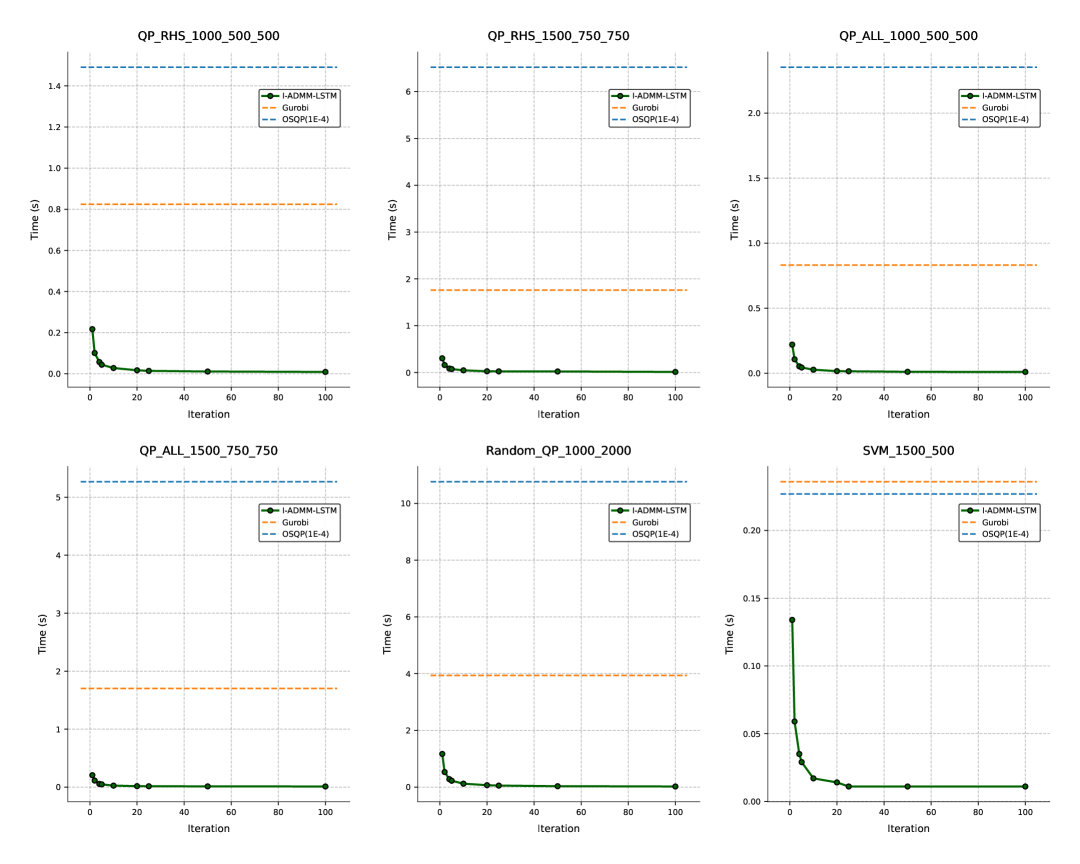
Figure 6: The time required for I-ADMM-LSTM to solve multiple optimization problems in parallel.

References

- Andrychowicz et al. (2016) Marcin Andrychowicz, Misha Denil, Sergio Gomez, Matthew W Hoffman, David Pfau, Tom Schaul, Brendan Shillingford, and Nando De Freitas. Learning to learn by gradient descent by gradient descent. Advances in neural information processing systems, 29, 2016.
- Applegate et al. (2021) David Applegate, Mateo Díaz, Oliver Hinder, Haihao Lu, Miles Lubin, Brendan O’Donoghue, and Warren Schudy. Practical large-scale linear programming using primal-dual hybrid gradient. Advances in Neural Information Processing Systems, 34:20243–20257, 2021.
- ApS (2019) Mosek ApS. Mosek optimization toolbox for matlab. User’s Guide and Reference Manual, Version, 4(1), 2019.
- Bai et al. (2025) Jianchao Bai, Miao Zhang, and Hongchao Zhang. An inexact admm for separable nonconvex and nonsmooth optimization. Computational Optimization and Applications, pages 1–35, 2025.
- Banjac et al. (2019) Goran Banjac, Paul Goulart, Bartolomeo Stellato, and Stephen Boyd. Infeasibility detection in the alternating direction method of multipliers for convex optimization. Journal of Optimization Theory and Applications, 183:490–519, 2019.
- Bellavia (1998) Stefania Bellavia. Inexact interior-point method. Journal of Optimization Theory and Applications, 96:109–121, 1998.
- Borrelli et al. (2017) Francesco Borrelli, Alberto Bemporad, and Manfred Morari. Predictive control for linear and hybrid systems. Cambridge University Press, 2017.
- Boyd et al. (2011) Stephen Boyd, Neal Parikh, Eric Chu, Borja Peleato, Jonathan Eckstein, et al. Distributed optimization and statistical learning via the alternating direction method of multipliers. Foundations and Trends® in Machine learning, 3(1):1–122, 2011.
- Boyd et al. (2013) Stephen Boyd, Mark T Mueller, Brendan O’Donoghue, Yang Wang, et al. Performance bounds and suboptimal policies for multi–period investment. Foundations and Trends® in Optimization, 1(1):1–72, 2013.
- Chen et al. (2022) Ziang Chen, Jialin Liu, Xinshang Wang, and Wotao Yin. On representing mixed-integer linear programs by graph neural networks. In The Eleventh International Conference on Learning Representations, 2022.
- Cortes (1995) Corinna Cortes. Support-vector networks. Machine Learning, 1995.
- Donti et al. (2021) Priya L Donti, David Rolnick, and J Zico Kolter. Dc3: A learning method for optimization with hard constraints. In International Conference on Learning Representations, 2021.
- Eisenstat and Walker (1994) Stanley C Eisenstat and Homer F Walker. Globally convergent inexact newton methods. SIAM Journal on Optimization, 4(2):393–422, 1994.
- Gao et al. (2024) Xi Gao, Jinxin Xiong, Akang Wang, Jiang Xue, Qingjiang Shi, et al. Ipm-lstm: A learning-based interior point method for solving nonlinear programs. Advances in Neural Information Processing Systems, 37:122891–122916, 2024.
- Garcia et al. (1989) Carlos E Garcia, David M Prett, and Manfred Morari. Model predictive control: Theory and practice—a survey. Automatica, 25(3):335–348, 1989.
- Gasse et al. (2022) Maxime Gasse, Simon Bowly, Quentin Cappart, Jonas Charfreitag, Laurent Charlin, Didier Chételat, Antonia Chmiela, Justin Dumouchelle, Ambros Gleixner, Aleksandr M Kazachkov, et al. The machine learning for combinatorial optimization competition (ml4co): Results and insights. In NeurIPS 2021 competitions and demonstrations track, pages 220–231. PMLR, 2022.
- Gregor and LeCun (2010) Karol Gregor and Yann LeCun. Learning fast approximations of sparse coding. In Proceedings of the 27th international conference on international conference on machine learning, pages 399–406, 2010.
- Greif et al. (2014) Chen Greif, Erin Moulding, and Dominique Orban. Bounds on eigenvalues of matrices arising from interior-point methods. SIAM Journal on Optimization, 24(1):49–83, 2014.
- Gurobi Optimization (2023) LLC Gurobi Optimization. Gurobi Optimizer Reference Manual, 2023. URL https://www.gurobi.com/documentation/.
- He et al. (2000) Bing-Sheng He, Hai Yang, and SL Wang. Alternating direction method with self-adaptive penalty parameters for monotone variational inequalities. Journal of Optimization Theory and applications, 106:337–356, 2000.
- He et al. (2014) Bingsheng He, Yanfei You, and Xiaoming Yuan. On the convergence of primal-dual hybrid gradient algorithm. SIAM Journal on Imaging Sciences, 7(4):2526–2537, 2014.
- Huber and Ronchetti (2011) Peter J Huber and Elvezio M Ronchetti. Robust statistics. John Wiley & Sons, 2011.
- Ichnowski et al. (2021) Jeffrey Ichnowski, Paras Jain, Bartolomeo Stellato, Goran Banjac, Michael Luo, Francesco Borrelli, Joseph E. Gonzalez, Ion Stoica, and Ken Goldberg. Accelerating quadratic optimization with reinforcement learning, 2021.
- John and Yıldırım (2008) Elizabeth John and E Alper Yıldırım. Implementation of warm-start strategies in interior-point methods for linear programming in fixed dimension. Computational Optimization and Applications, 41(2):151–183, 2008.
- Kim et al. (2023) Hongseok Kim et al. Self-supervised equality embedded deep lagrange dual for approximate constrained optimization. arXiv preprint arXiv:2306.06674, 2023.
- Kingma (2014) DP Kingma. Adam: a method for stochastic optimization. In Int Conf Learn Represent, 2014.
- Li et al. (2024) Bingheng Li, Linxin Yang, Yupeng Chen, Senmiao Wang, Haitao Mao, Qian Chen, Yao Ma, Akang Wang, Tian Ding, Jiliang Tang, et al. Pdhg-unrolled learning-to-optimize method for large-scale linear programming. In Proceedings of the 41st International Conference on Machine Learning, pages 29164–29180, 2024.
- Li et al. (2023) Meiyi Li, Soheil Kolouri, and Javad Mohammadi. Learning to solve optimization problems with hard linear constraints. IEEE Access, 2023.
- Liang et al. (2023) Enming Liang, Minghua Chen, and Steven Low. Low complexity homeomorphic projection to ensure neural-network solution feasibility for optimization over (non-) convex set. In Conference on Parsimony and Learning (Recent Spotlight Track), 2023.
- Lions and Mercier (1979) Pierre-Louis Lions and Bertrand Mercier. Splitting algorithms for the sum of two nonlinear operators. SIAM Journal on Numerical Analysis, 16(6):964–979, 1979.
- Liu et al. (2023) Jialin Liu, Xiaohan Chen, Zhangyang Wang, Wotao Yin, and HanQin Cai. Towards constituting mathematical structures for learning to optimize. In International Conference on Machine Learning, pages 21426–21449. PMLR, 2023.
- Lu and Yang (2023) Haihao Lu and Jinwen Yang. A practical and optimal first-order method for large-scale convex quadratic programming. arXiv preprint arXiv:2311.07710, 2023.
- Nair et al. (2020) Vinod Nair, Sergey Bartunov, Felix Gimeno, Ingrid Von Glehn, Pawel Lichocki, Ivan Lobov, Brendan O’Donoghue, Nicolas Sonnerat, Christian Tjandraatmadja, Pengming Wang, et al. Solving mixed integer programs using neural networks. arXiv preprint arXiv:2012.13349, 2020.
- O’Donoghue (2021) Brendan O’Donoghue. Operator splitting for a homogeneous embedding of the linear complementarity problem. SIAM Journal on Optimization, 31(3):1999–2023, 2021.
- O’donoghue et al. (2016) Brendan O’donoghue, Eric Chu, Neal Parikh, and Stephen Boyd. Conic optimization via operator splitting and homogeneous self-dual embedding. Journal of Optimization Theory and Applications, 169:1042–1068, 2016.
- Park and Van Hentenryck (2023) Seonho Park and Pascal Van Hentenryck. Self-supervised primal-dual learning for constrained optimization. In Proceedings of the AAAI Conference on Artificial Intelligence, volume 37, pages 4052–4060, 2023.
- Sambharya et al. (2023) Rajiv Sambharya, Georgina Hall, Brandon Amos, and Bartolomeo Stellato. End-to-end learning to warm-start for real-time quadratic optimization. In Learning for Dynamics and Control Conference, pages 220–234. PMLR, 2023.
- Stellato et al. (2020) Bartolomeo Stellato, Goran Banjac, Paul Goulart, Alberto Bemporad, and Stephen Boyd. Osqp: An operator splitting solver for quadratic programs. Mathematical Programming Computation, 12(4):637–672, 2020.
- Sun et al. (2016) Jian Sun, Huibin Li, Zongben Xu, et al. Deep admm-net for compressive sensing mri. Advances in neural information processing systems, 29, 2016.
- Tibshirani (1996) Robert Tibshirani. Regression shrinkage and selection via the lasso. Journal of the Royal Statistical Society Series B: Statistical Methodology, 58(1):267–288, 1996.
- Wächter and Biegler (2006) Andreas Wächter and Lorenz T Biegler. On the implementation of an interior-point filter line-search algorithm for large-scale nonlinear programming. Mathematical programming, 106:25–57, 2006.
- Xie (2018) Jiaxin Xie. On inexact admms with relative error criteria. Computational Optimization and Applications, 71(3):743–765, 2018.
- Xiu et al. (2023) Shengjie Xiu, Xiwen Wang, and Daniel P Palomar. A fast successive qp algorithm for general mean-variance portfolio optimization. IEEE Transactions on Signal Processing, 2023.