ARCANE - Early Detection of Interplanetary Coronal Mass Ejections

Abstract

Interplanetary coronal mass ejections (ICMEs) are major drivers of space weather disturbances, posing risks to both technological infrastructure and human activities. Automatic detection of ICMEs in solar wind in situ data is essential for early warning systems. While several methods have been proposed to identify these structures in time series data, robust real-time detection remains a significant challenge. In this work, we present ARCANE — the first framework explicitly designed for early ICME detection in streaming solar wind data under realistic operational constraints, enabling event identification without requiring observation of the full structure. Our approach evaluates the strengths and limitations of detection models by comparing a machine learning-based method to a threshold-based baseline. The ResUNet++ model, previously validated on science data, significantly outperforms the baseline, particularly in detecting high-impact events, while retaining solid performance on lower-impact cases. Notably, we find that using real-time solar wind (RTSW) data instead of high-resolution science data leads to only minimal performance degradation. Despite the challenges of operational settings, our detection pipeline achieves an F1 score of $0.53$, with an average detection delay of 21.5% of the event’s duration while only seeing a minimal amount of data. As more data becomes available, the performance increases significantly. These results mark a substantial step forward in automated space weather monitoring and lay the groundwork for enhanced real-time forecasting capabilities.

Space Weather

Austrian Space Weather Office, GeoSphere Austria, Graz, Austria Institute of Physics, University of Graz, Graz, Austria DPHY, ONERA, Université de Toulouse, 31000, Toulouse, France

H. T. Rüdisserhannah@ruedisser.at

We provide a modular framework to develop and evaluate methods for early detection of Interplanetary Coronal Mass Ejections in real-time.

We assess models under realistic operational conditions using streaming real-time solar wind data.

We reliably detect high-impact events in a real-time setting and achieve acceptable performance on low-impact events.

Plain Language Summary

Solar storms are major drivers of the weather in space, which can disrupt technology and impact our daily lives on Earth. Automatically recognizing these events in data from satellites near Earth is important for early warning systems, but current methods still have significant limitations. In this study, we present a new framework to evaluate how well different methods can automatically detect solar storms while observing the solar wind. We compare a machine learning model to a simpler threshold-based method. Our results show that the machine learning model performs much better, especially for identifying the most impactful events. Additionally, it still handles less critical events effectively. This system is a step forward for automated space weather monitoring and helps to improve real-time forecasting and early warning capabilities.

1 Introduction

Interplanetary coronal mass ejections (ICMEs) are among the primary drivers of space weather disturbances. These massive eruptions from the Sun occur more frequently during solar maximum [richardson_2012] and are responsible for the most intense geomagnetic storms [echer_2013]. Since their discovery in the $1970$’s [gosling_1973, Burlaga . (1981), klein_1982], ICMEs have been the subject of extensive research, with numerous studies focusing on their properties, propagation, and geoeffectiveness [<]e.g.¿[]kilpua_2017. These efforts have greatly advanced our understanding of their physical properties and have led to a number of publications of event catalogs, providing start and end times of ICMEs, as observed by various spacecraft [jian_2006, lepping_2006, richardson_2010, Chi_2016, nieves_chinchilla_2018, nguyen_automatic_2019, Möstl_2020, nguyen_multiclass_2025].

Interplanetary coronal mass ejections (ICMEs) are typically characterized by an enhanced, smoothly rotating magnetic field, a declining solar wind velocity, and low plasma beta ($\beta$), where $\beta$ is the ratio of thermal to magnetic pressure. They are often preceded by shocks and turbulent sheath regions, while their main structure is generally considered to be a magnetic cloud or flux rope. However, detecting ICMEs remains challenging due to the variability of their in situ signatures and the complex solar wind environment [<]e.g.¿[]zurbuchen_2006, Chi_2016, kilpua_2017. The observed signatures can vary significantly depending on factors such as the spacecraft trajectory through the ICME, interactions with other CMEs, or the presence of additional transient solar wind structures [<]e.g.¿kilpua2009, good2018correlation, Lugaz_2018, salman2020radial, ruedisser_2024.

Manually identifying ICME signatures is time-consuming and prone to inconsistencies. Catalogs often differ significantly, with studies showing that only a subset of the ICMEs in one catalog are present in another [<]e.g.¿[]rudisser_automatic_2022. This inconsistency is a major challenge for the development of automatic detection methods, as they rely on expert-labeled data for training and validation. However, automatically detecting these events in solar wind in situ data is essential for early warning systems, needed to mitigate the impact of space weather on critical infrastructure. A reliable ICME detection method could serve as a real-time trigger for more computationally intensive analysis, or even be deployed onboard a spacecraft to start different observational tasks.

Several approaches have been proposed to automate ICME detection. Traditional methods, such as threshold-based techniques [lepping_2005_automaticdetection], algorithms based on the Grad-Shafranov reconstruction technique [Hu_2018], and spatio-temporal entropy analysis [ojedagonzalez2017], have been employed. However, these approaches are highly dataset-dependent and often struggle to generalize across the diverse in situ signatures of ICMEs. More recent advancements in machine learning offer a promising alternative.

Early machine learning approaches for solar wind classification and ICME detection employed methods such as Gaussian Process classification and simple Convolutional Neural Networks (CNNs), demonstrating the feasibility of automated in situ data analysis [camporeale_classification_2017, nguyen_automatic_2019]. Subsequent advancements have leveraged deep learning architectures, such as UNets, to reframe ICME detection as a time series segmentation task [rudisser_automatic_2022, chen_ru-net_2022]. More recent efforts have explored alternative machine learning techniques, including feature selection with random forests to classify magnetic flux ropes [farooki_machine_2024], probabilistic neural networks for identifying solar wind structures [narock_classifying_2024], and supervised classification pipelines to further refine the automatic detection of magnetic flux ropes and solar transients [pal_automatic_2024].

The latest advancements integrate object detection frameworks inspired by the YOLO family [redmon_2016_yolo], enabling efficient multi-class event detection with minimal post-processing. These approaches unify the identification of ICMEs and Stream Interaction Regions (SIRs) within a single model, achieving high precision and recall in extensive datasets [nguyen_multiclass_2025].

Despite the substantial advancements in automatic detection of large-scale structures in solar wind in situ data, significant challenges remain in the field. One of the primary complications is the inherent subjectivity and inconsistency in existing event catalogs. As highlighted in previous work, the identification of ICMEs is still heavily dependent on expert visual labeling, which is time-consuming and highly biased [rudisser_automatic_2022].

In addition to the challenges stemming from incomplete catalogs, there are several difficulties when applying automatic detection methods in operational real-time settings. One potential issue is the difference in data quality. While many of the models discussed above are trained, validated, and tested on science-quality data, real-time data is often of lower quality, with increased noise and potentially containing more gaps. Another challenge arises from the fact that many current detection methods rely on analyzing the entire time series before identifying an ICME and setting its boundaries. However, in an operational setting, the goal is to detect events as early as possible with sufficient confidence to avoid false alarms. This means that the model must be capable of identifying initial signs of an ICME, such as the shock, sheath, or the early onset of the magnetic cloud, even when only part of the data is available.

In this study, we introduce ARCANE (Automatic Real-time deteCtion ANd forEcast), a comprehensive and modular machine learning framework designed for the real-time detection, prediction, and analysis of interplanetary coronal mass ejections (ICMEs) using solar wind in situ data. By integrating multiple state-of-the-art methods across different stages, ARCANE provides an automated, data-driven, and physics-informed system for space weather forecasting and operational early warning.

Here, we focus on the first component of ARCANE: the early detection of ICMEs. In contrast to rudisser_automatic_2022, which evaluated ICME detection retrospectively, we assess our model under realistic operational conditions, emphasizing evaluation methodologies specifically designed to measure its capability to detect ICMEs in a real-time scenario.

The structure of this paper is as follows: Section 2 describes the datasets used in this study, including in situ solar wind measurements, event catalogs, and the generation of labels. Section 3 outlines the detection module of ARCANE, detailing model architecture, training process, and the baseline model we compare to. Additionally, we introduce postprocessing and evaluation strategy and validate this approach. Section 4 presents our experimental results, comparing the performance of our model against the baseline and assessing its early detection capabilities. Finally, in Section 5, we discuss the implications of our findings for operational space weather forecasting and outline possible directions for future research.

2 Data

2.1 In Situ Data

In previous work [rudisser_automatic_2022], we utilized solar wind in situ data from Wind, STEREO-A and STEREO-B, with varied input parameters. nguyen_multiclass_2025 and many other machine learning studies made use of the OMNI dataset [King_Papitashvili_2005], as it provides preprocessed, 1-minute-resolution data, specifically intended to support studies of the effects of solar wind variations on the magnetosphere and ionosphere. Data is available from 1995 onward. However, its lack of real-time availability renders it unsuitable for operational space weather forecasting.

To address this limitation, we rely on the NOAA Real-Time Solar Wind (RTSW) dataset [zwickl_noaa_1998], which is made available by the Space Weather Prediction Center (NOAA SWPC) and accessible at https://www.spaceweather.gov/products/real-time-solar-wind, as shown in Figure 1. This archived dataset comprises measurements from various spacecraft located upstream of Earth, typically at the L1 Lagrange point, and tracked by the Real-Time Solar Wind Network of ground stations. Data is available from 1998 onward, with the NOAA/DSCOVR satellite [Burt  Smith (2012)] serving as the primary operational RTSW spacecraft since July 2016, replacing the NASA/ACE spacecraft [Chiu1998_ace]. However, in the event of issues with DSCOVR, the NASA/ACE spacecraft resumes its role as the operational RTSW source, serving as a backup. During such periods, RTSW data is provided by four ACE instruments: EPAM - Energetic Ions and Electrons [EPAM_Gold_Krimigis_Hawkins_Haggerty_Lohr_Fiore_Armstrong_Holland_Lanzerotti_1998], MAG - Magnetic Field Vectors [MAG_Smith_1998], SIS - High Energy Particle Fluxes [SIS_Stone_1998], and SWEPAM - Solar Wind Ions [SWEPAM_Comas_1998]. The two DSCOVR instruments for which real-time data is available are the magnetometer (MAG) and the Faraday Cup (FC) [lotoaniu_validation_2022].

To mimic a real-time operational scenario, we compile a dataset by selecting data from the spacecraft designated as operational during specific periods.

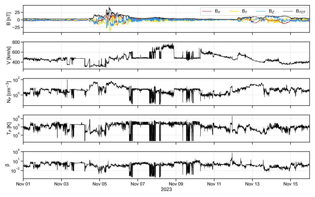
Figure 1: This figure shows the RTSW data as available via NOAA SWPC. The top panel shows the total magnetic field $B_{TOT}$, along with the vector components $B_{X}$, $B_{Y}$, and $B_{Z}$ in GSM coordinates. The remaining panels show from top to bottom: the bulk velocity $V$, the proton density $N_{P}$, proton temperature $T_{P}$, and plasma $\beta$.

The DSCOVR MAG and FC data have been validated against equivalent science-quality data from Wind and ACE. The results demonstrate strong statistical agreement in both magnetic field measurements and the velocity components relevant to this study [lotoaniu_validation_2022]. Similarly, Lugaz_2018 highlighted a sufficiently high correlation in magnetic ejecta measurements between ACE and Wind, supporting the interchangeability of these datasets when referencing event catalogs.

Beyond data validation, Bouriat_2022 explored the usability of ACE data for machine learning applications. While challenges such as data gaps were identified, their study suggested that integrating ACE with DSCOVR observations could help mitigate missing values, making these datasets more robust for predictive modeling. A related investigation by smith2022 assessed the suitability of near-real-time (NRT) data for space weather forecasting. Their findings indicate that while NRT datasets are valuable for real-time hazard prediction, they exhibit increased short-term variability and occasional anomalies when compared to post-processed, science-quality data.

Despite these limitations, certain parameters in NRT data remain reliable, according to smith2022. For instance, solar wind velocity typically deviates by no more than $\pm 10\%$ from the post-processed data. Similarly, density and temperature measurements are generally consistent with science-quality data but may display greater uncertainty. Magnetic field measurements show a comparable level of variability, with total field magnitudes typically accurate within $\pm 10\%$ of their processed values. While smith2022 suggest that some models might be able to overcome these issues when being trained directly on NRT data, others may require additional preprocessing steps.

In situ measurements often consist of a wide range of input parameters provided by different instruments. nguyen_automatic_2019 demonstrated that incorporating all available parameters, including 15 channels of proton fluxes, resulted in slight improvements compared to using only magnetic field data and general plasma parameters. However, pal_automatic_2024 focused solely on magnetic field measurements, and both rudisser_automatic_2022 and nguyen_multiclass_2025 successfully used a limited number of input variables without affecting detection performance.

In this study, we focus on a limited number of input variables to ensure compatibility across different spacecraft. Following nguyen_multiclass_2025, we select the following parameters: the three Geocentric Solar Magnetic (GSM) components of the interplanetary magnetic field (IMF) ($B_{X}$, $B_{Y}$, $B_{Z}$), their total magnitude ($B$), the proton density ($N_{p}$), the proton temperature ($T_{p}$), the bulk solar wind speed ($V$), and the plasma beta ($\beta$). This results in a total of six independent parameters, while $B$ is derived from the individual magnetic field components and $\beta$ is calculated using $N_{p}$, $T_{p}$, and $B$.

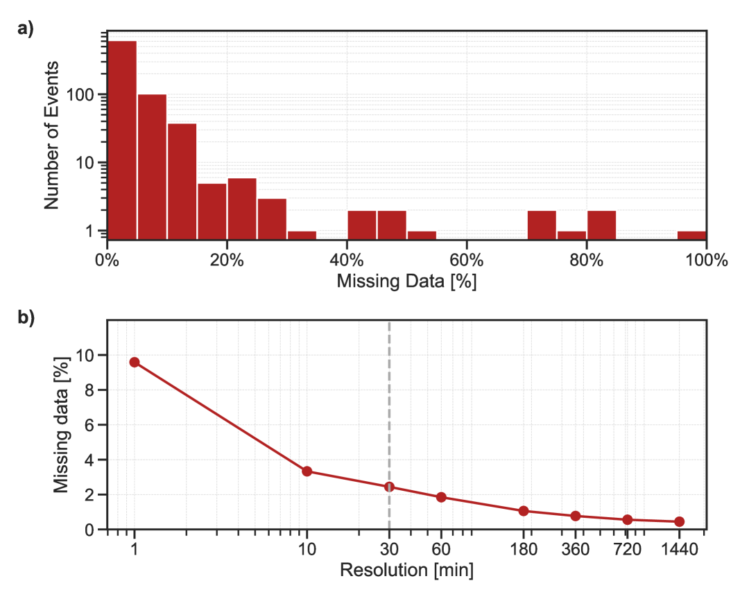
Figure 2: Overview of missing data characteristics in the RTSW dataset. (a) Missing data percentage per ICME event for the RTSW dataset. The bars show the histogram of missing data per ICME event. (b) Percentage of missing data depending on the chosen resolution for both the RTSW dataset. The dashed vertical grey line indicates the resolution we opted for.

Figure 2a illustrates the percentage of missing data per ICME event for the RTSW dataset. As expected, the RTSW dataset exhibits a significant proportion of missing data. Despite these limitations, we train on the RTSW dataset to enable the model to adapt to and learn from lower-quality data. Our tests have shown that this strategy enhances the model’s robustness and overall performance compared to training on a science-quality dataset, such as the OMNI dataset.

The complete RTSW dataset comprises approximately $1.23\times 10^{7}$ data points between 1998-02-16 00:00:00 and 2023-12-17 04:00:00, with a resolution of $1$ minute and about $9.59\%$ missing values. To address this, nguyen_automatic_2019 and rudisser_automatic_2022 resampled all in situ data to a $10$-minute resolution. Figure 2b shows the percentage of missing data, depending on the chosen resolution.

For this study, a $30$-minute resolution was selected to balance minimizing data gaps with maintaining sufficient temporal resolution for early warning and detection. This resampling strategy effectively reduced the proportion of missing values to approximately $2.44\%$ in the RTSW dataset. Additionally, this approach inherently accounts for uncertainties in event boundaries and mitigates the impact of short-term data gaps. To further improve data continuity, we applied linear interpolation for gaps shorter than 6 hours, reducing the proportion of missing values to $<1$ %.

As proposed in rudisser_automatic_2022, a sliding window method was applied to segment the time series and associated labels into fixed-length windows of $512$ timesteps. At the chosen resolution of $30$ minutes, each window corresponds to a little over $10.5$ days. A stride of $1$ was used to simulate a real-time operational environment. Finally, any windows that still contain missing values are discarded. This resulted in $404403$ samples for the RTSW dataset.

We normalize and scale the data such that each feature has a mean of $0$ and a standard deviation of $1$. To preserve the relative magnitudes of the magnetic field components, the four magnetic field values ($B_{X}$, $B_{Y}$, $B_{Z}$, $B_{TOT}$) are treated as a single feature during the scaling process.

2.2 Event Catalogs

As extensively discussed in prior studies, ICME catalogs often differ in their identification criteria, leading to variations in both the number of recorded events and their reported start and end times. For this study, we use an updated version of the aggregated ICME catalog introduced by nguyen_multiclass_2025, which consolidates entries from richardson_2010, moestl_2017, nieves_chinchilla_2018 and nguyen_automatic_2019, adapted for OMNI data. While these catalogs are not entirely exhaustive, as noted in nguyen_automatic_2019, they remain among the most comprehensive resources currently available.

After filtering out events with remaining data gaps, the catalog provides a total of 681 events for the period under study. Although this catalog was specifically adapted for OMNI data, we disregard the time shift between OMNI and RTSW data, as the  40-minute difference falls within the uncertainty of event boundaries introduced by our sampling strategy.

Furthermore, we choose to include the sheath region—when present—as part of the ICME structure. This decision is consistent with the approach taken by nguyen_multiclass_2025. Although there is no universally accepted definition regarding whether the sheath should be considered part of the ICME, we argue for its inclusion based on both practical and scientific considerations. Sheath regions are often geoeffective and can significantly contribute to space weather disturbances. As highlighted by riley_2023, they can also provide valuable early indicators for forecasting key ICME parameters. Especially in a real-time operational context, this makes the sheath a relevant and informative component for analysis.

2.3 Generation of Labels

To generate the labels for the time series segmentation task, we process the catalog, following the approach described in rudisser_automatic_2022. Specifically, we create a binary time series where each timestep is labeled as 1 if it falls within an event and 0 otherwise. In future work, this could be adapted to assigning different values to the sheath and the flux rope part of the ICME. The start and end times of the events have been rounded to the chosen resolution of $30$ minutes.

Windows were classified as positive if the last timestep fell within an ICME event and was therefore labeled as $1$. An example pair of input and output is shown in Figure 3.

Using this criterion, the proportion of positive samples, corresponding to having the last timestep in the window labeled as ICME, was calculated to be $12.58\%$ for the RTSW dataset.

3 Framework and Methodology

In this section, we introduce the setup of our framework, ARCANE (Automatic Real-Time deteCtion ANd forEcast), along with its early detection module. ARCANE serves as a highly modular and adaptable machine learning framework created to address the complexities of time series event detection tasks. Its primary goal is to streamline workflows by offering integrated modules and tools for data preprocessing, model training, testing, evaluation and visualization.

The framework is built on Hydra [Yadan2019Hydra], which provides a flexible and modular setup, making it easy to configure and manage experiments. The configurable components are organized into eight main categories: Datasets, Boundaries, Callbacks, Collates, Models, Modules, Samplers, and Schedulers. Each module can be adjusted directly through configuration files, allowing for quick modification of setups without altering the core code.

These modules integrate with available scripts, which handle tasks such as training, testing, analysis and prediction. The framework also includes routines specifically designed to download and process the RTSW data.

3.1 Model Architecture

The used model is a modified ResUNet++ architecture, as described in rudisser_automatic_2022, which achieved state-of-the-art performance for the automatic detection of ICMEs. nguyen_multiclass_2025 compared this architecture to their YOLO-based approach, ”SPODIfY,” finding comparable results between the two methods. The main difference lies in the output representation: while YOLO-based models rely on bounding boxes to localize events, ResUNet++ performs pointwise segmentation. Since our focus lies on early detection in streaming data – in which events unfold progressively and are not fully visible from the start – segmentation proves more effective than bounding boxes, which may struggle to capture the gradual onset of an ICME. Initial tests confirmed that ResUNet++ is better suited for our goals, demonstrating superior performance in predicting event boundaries at an early stage.

While the original implementation in rudisser_automatic_2022 used 2D convolutional layers, we adapted the architecture to use 1D convolutions, reflecting the structure of our dataset. Additionally, we adjusted the filter sizes from $[64,128,256,512]$ to $[32,64,128,256]$. The lower resolution of our dataset justifies this reduction in filter sizes and results in a significant decrease in the number of trainable parameters, enhancing computational efficiency without compromising performance. For a complete description of all the components of the model, see rudisser_automatic_2022.

The architecture of our modified ResUNet++ model is shown in Figure 3.

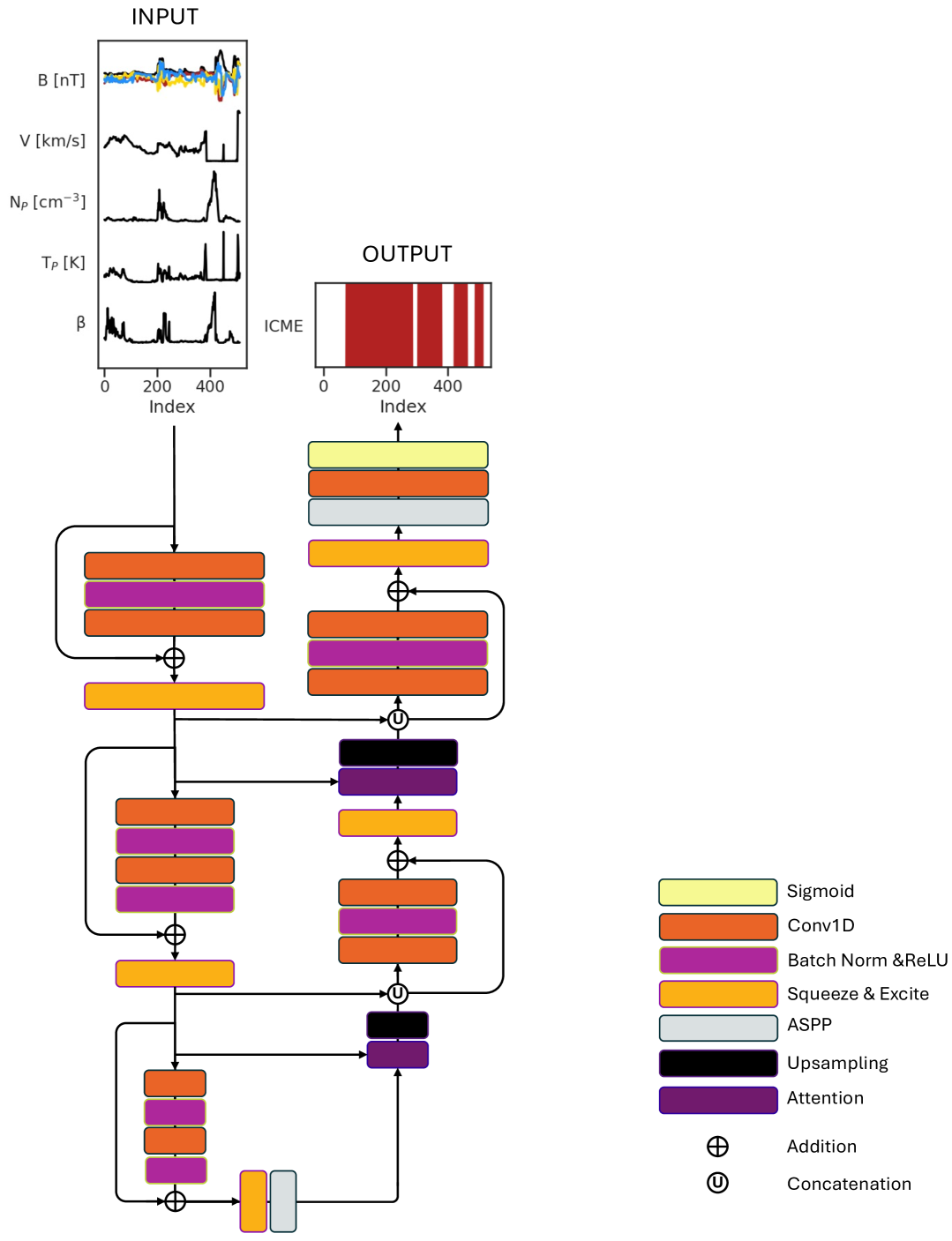
Figure 3: Schematic representation of the used model, adapted from rudisser_automatic_2022. A complete description of the used layers and components can be found in rudisser_automatic_2022. Additionally, we show a sample from the dataset, containing an example input and output. The input consists of 8 variables. From top to bottom: Magnetic field $B$ plus components $B_{X}$, $B_{Y}$, $B_{Z}$, bulk velocity $V$, proton density $N_{P}$, proton temperature $T_{P}$ and plasma $\beta$. The output is a segmented time series that consists of $0$ (white) and $1$ (red), depending on whether a point in time contains an ICME event or not.

3.2 Training

To address our limited dataset size, we employ the nested cross-validation strategy outlined by bernoux_2022_geomagforecast. The dataset is divided into yearly folds, with each fold serving as a test set while the remaining folds are used for training and validation. For each test year, the remaining years are further split into three equal subsets. Two-thirds are used for training, while the remaining third functions as a validation set. To ensure a fair evaluation, we repeat this process three times, cycling through which subset is designated as validation data. The final prediction for the test set is obtained by averaging the predictions of the three resulting models, thereby reducing variance and enhancing stability.

This two-loop evaluation approach ensures unbiased evaluation, mitigating the limitations of simpler cross-validation techniques. Although it requires training multiple models, this method enhances the robustness of our results and enables performance assessment across different solar cycle phases. To prevent data leakage between the training, validation, and test sets, we exclude frames near boundaries.

During training, we minimize the Dice Loss [jadon_2020], with a smoothing factor of one, using the Adam optimizer [kingma2014_adam]. The model is trained for a maximum of $100$ epochs with an initial learning rate of $10^{-3}$, which is reduced by a factor of $0.1$ if the validation loss does not improve for $3$ epochs. Early stopping halts training after $10$ epochs of no improvement. To account for the class imbalance, we adopt a weighted sampling approach. The probability of drawing a sample with a positive label at the last timestep is 10 times higher than for a negative sample. We use a batch size of $128$, and training samples are shuffled after each epoch. These hyperparameters have been fine-tuned through extensive optimization.

On an NVIDIA GeForce RTX 4090, 24GB GPU, one epoch takes less than $4$ minutes and the model typically converges in less than 10 epochs.

3.3 Baseline

We implemented a simple baseline to compare our results to. lepping_2005_automaticdetection introduced several prediction criteria to identify ICMEs in solar wind in situ data. Their classification scheme is divided into two parts: the first part focuses on the identification of ICME characteristics on short time scales ($>$ 30 minutes) and the second part on the identification on longer time scales ($>8$ hours). To avoid introducing a minimal waiting time of $8$ hours and simultaneously be able to perform a pointwise comparison, we focus on the first part of their classification scheme, which is based on the following criteria: the running average of proton plasma beta must be low ($<~\!\!\!\beta_{p}\!\!\!~>_{L}\ \ \leq 0.3$), the direction of the magnetic field must change slowly (quadratic fitting of $\Theta_{B}$ (latitude) with $\chi^{2}\leq 450$), the average of the magnetic field magnitude $<\!\!|B|\!\!>$ must be $\geq 8.0$ nT, the average proton thermal velocity $<~\!\!|V_{Th}|\!\!~>$ must be $\leq 30$ km s^-1and the latitudinal difference angle of the magnetic field, $\Delta\Theta_{B}$ must be $\geq 45$ ^∘.

To adapt these criteria for a real-time setting, we define the following thresholds:

• $B_{max}\geq 8$ nT

• $\beta\leq 0.3$

• $T_{p}\leq 4.3\times 10^{4}$ K

The threshold for $T_{p}$ is derived from the equation:

$$T=\frac{\pi m_{p}V_{Th}^{2}}{8k_{B}}$$ (1)

where $k_{B}$ is the Boltzmann constant and $m_{p}$ is the proton mass. The value is rounded up for simplicity. During inference, each time step in the dataset is analyzed individually to determine whether it meets all the conditions required to classify it as an event.

3.4 Postprocessing

During inference, the original ResUNet++ model processes data in sliding windows and outputs a time series of values between zero and one for each window. To evaluate the model’s ability to detect events early, we extract the model’s prediction at the last time step of each window and stack them to obtain a time series. This extracted time series, denoted as $t_{1}$, represents the classification decision that would be made as soon as a new point in time enters the window. This approach simulates real-time classification, where decisions must be made without waiting for future data.

To systematically analyze how early the model can reliably detect an event, we extend this approach to earlier time steps within the window. Specifically, we extract predictions at progressively later time steps, denoted as $t_{2}$ through $t_{50}$. Each of these corresponds to a different waiting time $\delta$, which we define as the duration for which a point in time has been observed before being classified. Per definition, $t_{2}$ accounts for the prediction that has been made after observing a point in time for $\delta(t_{2})=1$ hour, taking into account an additional data point and $t_{50}$ accounts for the prediction after $\delta(t_{50})=25$ hours.

This method produces 50 different time series, each representing the model’s predictions at a specific waiting time $\delta$. By analyzing these series, we can study how detection performance evolves as more data becomes available. A schematic representation of this process is shown in Figure 4.

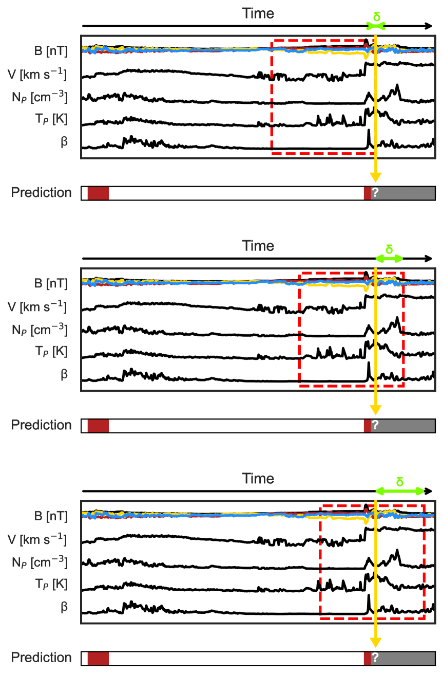
Figure 4: Schematic illustration of the postprocessing method used to extract 50 different time series of predictions at varying waiting times $\delta$. Each subplot represents a single prediction time step for a specific $\delta$ value. The red dashed rectangle indicates the sliding window of input data provided to the model. The yellow vertical arrow marks the current time step being classified as either CME or no CME. The horizontal strip below each plot labeled Prediction represents the full prediction time axis: segments before the prediction point correspond to previous predictions (red to indicate positive predictions), while the gray segment under and after the yellow arrow indicates time steps that have not yet been predicted. The neon green double-headed arrow labeled $\delta$ shows the gap between the end of the input window and the current prediction time step, defining the waiting time: how long the model “waits” before making a prediction about a point in time. By shifting the prediction point further from the input window (increasing $\delta$), we can assess how the model’s detection performance evolves with seeing more future data before making a prediction.

The final postprocessing steps are identical for both the ARCANE Classifier and the Threshold Classifier baseline. To convert each time series into a list of events $E$, we apply a simple thresholding approach for a range of thresholds between $0.1$ and $1.0$. Consecutive time steps exceeding the threshold are grouped into a single event.

To ensure practical applicability, we discard events with a duration of $\leq 30$ minutes, as these would not be detected in a real-time setting. Additionally, events separated by $\leq 30$ minutes are merged into a single event. The final boundaries of the detected events $E_{d}$ are determined by the first ($t_{s}(E_{d})$) and last ($t_{e}(E_{d})$) time step that exceeds the threshold.

nguyen_multiclass_2025 used a slightly different approach only applicable in a non-real-time scenario. Their method applied a fixed threshold of $0.1$, and the detection probability of each event was computed as the mean probability within its detected boundaries. While we compared our results to theirs by replicating their postprocessing approach as a benchmark, we primarily rely on our own postprocessing method, better suited to our real-time detection requirements.

3.5 Evaluation

In the postprocessing step, we generate a list of detected events, denoted as $E_{d}$, and compare it to the list of ground truth events $E_{t}$. For each ground truth event, we check whether it overlaps with any detected event. If an overlap is found, the ground truth event is counted as a true positive (TP). In cases where multiple detected events overlap with a single ground truth event, only the first overlapping detected event is assigned as a true positive; the remaining overlaps are ignored for this event. If a ground truth event does not overlap with any detected event, it is considered a false negative (FN). Conversely, any detected event that does not overlap with a ground truth event is counted as a false positive (FP).

We calculate the standard metrics Precision, Recall and F1-Score to evaluate the model’s performance:

$$\text{Precision}=\frac{\text{TP}}{\text{TP}+\text{FP}}$$ (2)

$$\text{Recall}=\frac{\text{TP}}{\text{TP}+\text{FN}}$$ (3)

$$\text{F1}=2\times\frac{\text{Precision}\times\text{Recall}}{\text{Precision}+\text{Recall}}$$ (4)

To specifically assess the model’s ability to detect events early, we introduce a new metric, ”Delay”. This metric measures the time difference between the actual start time of a ground truth event $t_{s}(E_{t})$ and the time of its first detection, where the first detection corresponds to the time step $t_{s}(E_{d})$, at which the threshold is exceeded for the first time. To account for the model’s prediction delay, we add the time series’ waiting time parameter $\delta$ to the detected events’ start time:

$$\text{Delay}=\text{max}((t_{s}(E_{d})-t_{s}(E_{t}),0)+\delta$$ (5)

This definition ensures that early or perfectly timed detections result in a Delay equal to the waiting time $\delta$, while late detections are penalized by the additional time lag. The max function ensures that early detections do not lead to artificially negative or reduced Delay values, since in operational practice, an early alert is still subject to the waiting time $\delta$.

Finally, we also report the error on start time, corresponding to the absolute value $|(t_{s}(E_{t})-t_{s}(E_{d})|$.

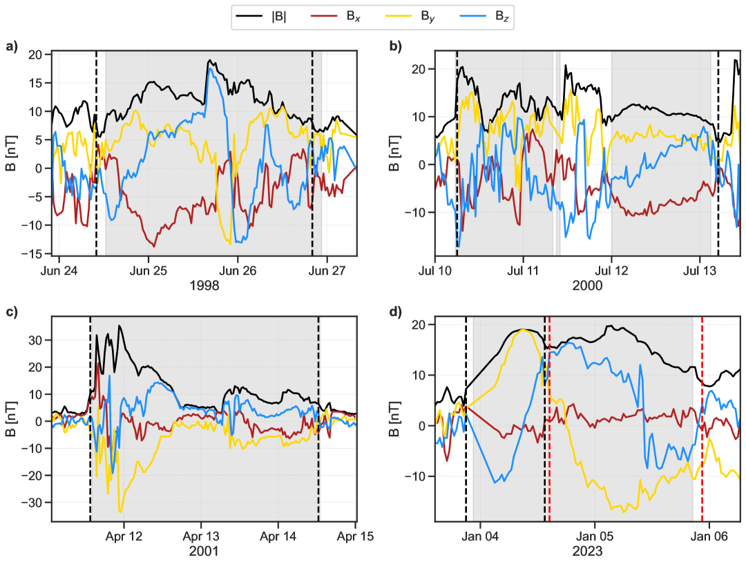
Figure 5: Four examples showing both the ground truth and the prediction made by ARCANE. The total magnetic field $B_{TOT}$ along with its vector components $B_{X}$, $B_{Y}$ and $B_{Z}$ are displayed, with the grey shaded area corresponding to the events predicted by ARCANE and the vertical black and red lines denoting the start and end time of the respective ground truth events. (a) Correctly predicted event with a small error on the start time. (b) Single ground truth event predicted through multiple events. (c) Correctly predicted event with no error on the start time. (d) Multiple ground truth events predicted through a single event.

Figure 5 illustrates multiple scenarios in which these considerations are particularly important. Figure 5a shows a correctly predicted event with a small error on the start time. Figure 5b shows a single ground truth event, for which two predicted events are detected. The second predicted event is not counted as an additional true positive to avoid overestimating the overall Precision. This choice reflects the logic of a real-time detection setting, where the first prediction would have already triggered an alert. Any further predictions for the same event are considered redundant.

Figure 5c shows a correctly predicted event with no error on the start time. Figure 5d shows a case where two distinct ground truth events are both detected by the same predicted event. In this case, the start time error for each ground truth event is measured as the difference between the beginning of the predicted event (shaded region) and the respective true start times, denoted by the vertical black (first event) and red (second event) lines. This leads to a larger start time error for the second event. However, the Delay for the second event is defined as $\delta$, since the contribution of the error on the start time to the Delay cannot be negative.

3.6 Validation of Postprocessing and Evaluation

To test the validity of this approach, we attempt to regenerate the catalog from our created labels and evaluate the two catalogs against each other. This analysis is conducted to verify that the forward and backward mapping between the generated time series and the event catalog works as expected. We calculate the Precision, Recall and F1-Score for the generated catalog and compare it to the ground truth catalog. Figure 6 shows the number of events over the entire dataset for both the ground truth and the generated catalog.

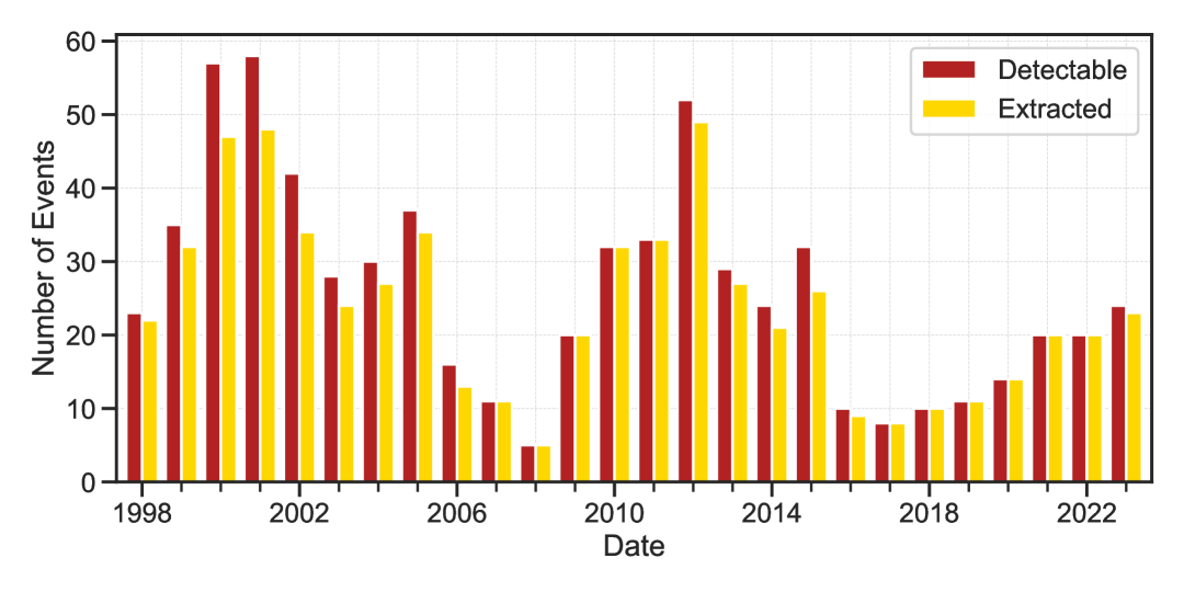
Figure 6: Number of events over the entire RTSW dataset for both the ground truth (detectable) and the generated catalog (extracted). The dependence of the number of events on the solar cycle of $11$ years is clearly visible.

As expected, the number of events in the generated catalog is lower as the approach combines nearby events into a single event. Our approach is supposed to allow for this behavior without penalizing it in the evaluation if only one of these nearby events is detected. In the case of the RTSW dataset, there are $681$ events to be detected. Extracting $620$ events during the postprocessing step, the evaluation yields a perfect Precision, Recall, and F1-Score of $1.0$. As these merged events cannot be distinguished, we treat the generated catalog as our ground truth moving forward.

4 Results

4.1 Detection Performance and Delay

To ensure comparability with previous studies, we calculate Precision, Recall, and F1-Score following the approach used by nguyen_multiclass_2025. Their study reported that SPODIfY achieved a maximum F1-Score of $0.784$, while ResUNet++ reached $0.782$, both trained and evaluated on OMNI data. In comparison, our model attains a maximum F1-Score of $0.745$. While performance on the RTSW dataset is slightly lower than these benchmarks, the decline is likely due to data gaps and the limited number of training years available in RTSW. Nonetheless, these results highlight the potential of RTSW data for real-time applications, reinforcing its suitability for operational use.

Following our own postprocessing routine as explained earlier, we generate an event catalog from the model’s predictions and compare it to the ground truth catalog for each of the $50$ time series, based on different waiting times $\delta$. Precision and Recall are calculated across a range of thresholds for each time series and the resulting Precision-Recall curves are shown in Figure 7a, where the color indicates the waiting time $\delta$ in hours. The curves are horizontally extended as dashed lines for better comparability. The performance of the Threshold Classifier baseline is indicated as a blue rectangle for comparison.

As anticipated, longer waiting times result in higher Precision values, as the model is exposed to a larger portion of the event by that point in time. However, this improvement appears to be relatively modest after the initial hours have passed. Interestingly, shorter waiting times yield slightly higher Recall. This observation aligns with the model’s tendency to generate optimistic alerts based on small variations when it has seen only a fraction of an event. Over time, as more data becomes available, the model refines its predictions, reducing the number of false positives and thereby increasing Precision.

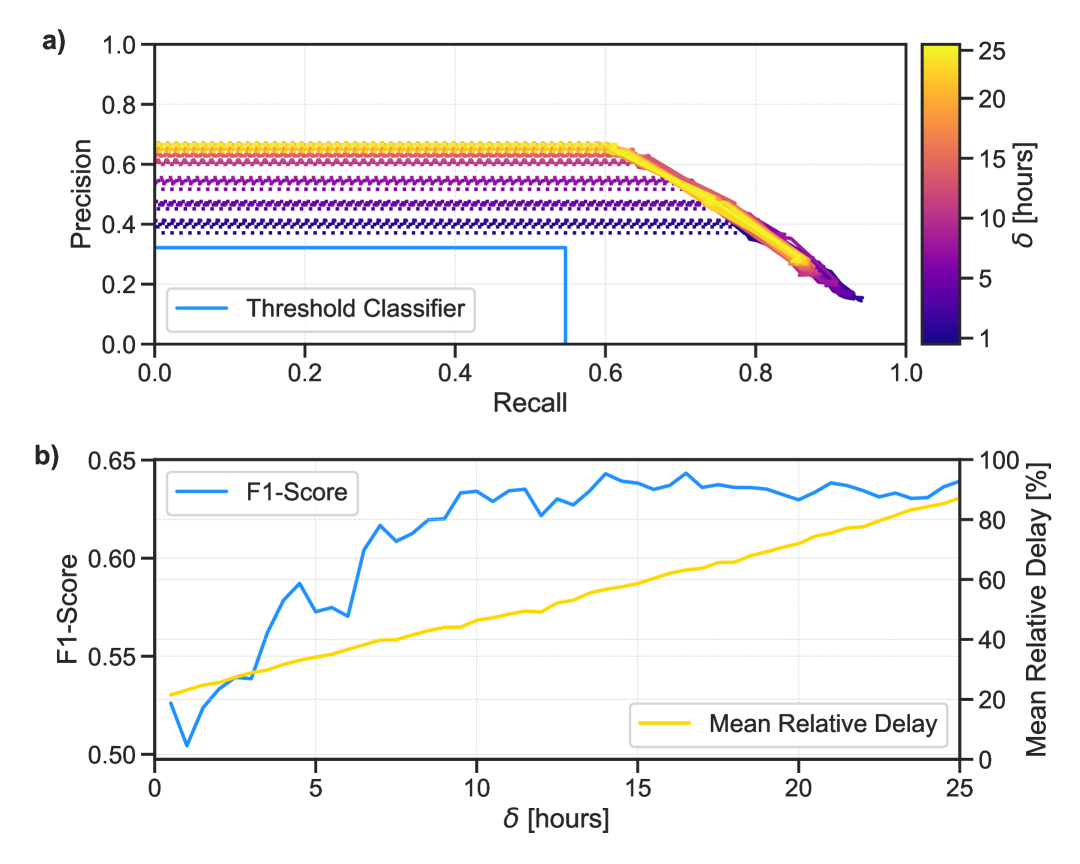
Figure 7: Overview of detection performance as a function of waiting time $\delta$. (a) Precision-Recall curves for each time series. The color indicates the waiting time $\delta$ in hours. The performance Threshold Classifier baseline is indicated as a blue rectangle for comparison. (b) F1-Score and mean relative Delay in percentage of the duration as a function of the waiting time $\delta$.

Additionally, we compute the maximum F1-score for each waiting time $\delta$ and present it as a function of $\delta$ in Figure 7b. This figure highlights the clear dependence of model performance on the waiting time. While waiting for extended periods is impractical in a real-time scenario, it is encouraging to observe that the performance becomes acceptable after just a few hours. This indicates that the model can achieve reliable early detection without significant delays, which is critical for real-time operational use.

We summarize the maximum Precision, Recall, and F1-Score for four different waiting times of the ARCANE Classifier and the Threshold Classifier baseline in Table LABEL:tab:eventwise_results. Additionally, we show the absolute and relative mean error on the start time.

Table 1: Precision, Recall, F1-Score, Absolute Mean Error (AME) on the Start Time, Relative Mean Error (RME) on the Start Time, Mean Delay (MD) and Relative Mean Delay (RMD) for different waiting times of the ARCANE Classifier and the Threshold Classifier baseline.

	Prec.	Rec.	F1	AME [h]	RME [%]	MD [h]	RMD [%]
ARCANE ($\delta=0.5$h)	0.40	0.77	0.53	8.6	21.5	8.23	21.5
ARCANE ($\delta=3.0$h)	0.41	0.78	0.54	8.1	22.3	10.3	28.9
ARCANE ($\delta=6.0$h)	0.47	0.74	0.57	7.4	19.9	12.6	36.6
ARCANE ($\delta=12.0$h)	0.59	0.66	0.62	6.8	17.1	17.7	49.2
Threshold Classifier	0.32	0.55	0.41	13.4	29.1	13.2	28.6

We further evaluate the model’s ability to detect events early by calculating the delay parameter for each event and waiting time. The mean relative delay for each waiting time is shown in Figure 7 b) and exhibits a linear relationship, as expected. The waiting time has the most significant impact on the delay, highlighting the importance of early event detection. At the same time, we observe that the error made on the start time of the event stays more or less constant and is only slightly refined as the model sees more of the event. While the F1-score increases substantially within the first few hours, the mean delay also rises, which is crucial to minimize when it comes to operational space weather monitoring.

To quantify this performance, we calculate both the mean and relative mean of the Delay parameter for four different waiting times. These metrics are also computed for the Threshold classifier baseline, with the results summarized in Table LABEL:tab:eventwise_results.

The cumulative distribution of these delays for different waiting times is shown in Figure 8. As expected, the cumulative number of detected events rises steeply at lower delay values before leveling off at higher delays. The ARCANE classifier consistently achieves a higher cumulative number of detected events at higher delay values compared to the Threshold classifier, reflecting its superior recall.

At a waiting time of $\delta=0.5$h, the ARCANE classifier outperforms the baseline across all delay values, demonstrating its ability to detect events earlier. However, at higher waiting times, the ARCANE classifier exhibits larger delay values than the Threshold classifier. Nevertheless, this increased delay is accompanied by a higher F1-score, as shown in previous results, indicating a trade-off between detection performance and timeliness.

It is important to note that these delay values were calculated using a threshold optimized for maximizing the F1-score. Adjusting the threshold further impacts the delay, allowing for a trade-off between detection performance and timeliness. By lowering the threshold of the ARCANE classifier, one could prioritize earlier event detection at the expense of a reduced F1-score, offering additional flexibility depending on operational requirements.

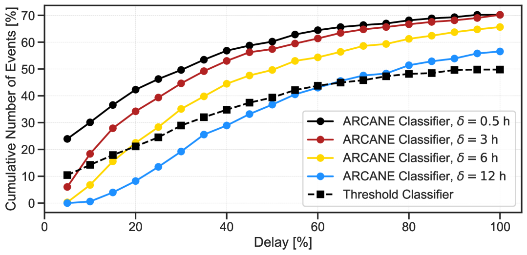
Figure 8: Cumulative distribution of the Delay values for the ARCANE Classifier at different waiting times and the Threshold Classifier baseline. The Delay is given in percentage of the event duration.

4.2 Analysis of Key Parameters

To better understand the characteristics of the true positive (TP), false positive (FP), and false negative (FN) events at a waiting time of $0.5$h, we analyze key event parameters and their interdependencies. Specifically, Figure 9 visualizes the relationship between the maximum value of $B_{TOT}$ and the maximum value of $V$ for each event, alongside their kernel density estimates (KDEs).

Figure 9: Maximum value of $B_{TOT}$ against maximum value of $V$ for TP, FP and FN events. Additionally, the kernel density estimation for each group of events is given.

Our analysis reveals that events with high peak $B_{TOT}$ values are consistently detected, highlighting the model’s ability to effectively capture strong magnetic field structures. Since ICMEs with large magnetic field strengths are more geoeffective, detecting these events is particularly important. Notably, most FN events exhibit peak $B_{TOT}$ values below 20 nT, with a significant fraction below 10 nT. Similarly, undetected events tend to have lower velocities, predominantly below 600 km s^-1. Given that weaker magnetic field strengths and lower velocities are generally associated with less impactful ICMEs, the model’s focus on high-impact events aligns well with operational forecasting priorities.

These results indicate that the model successfully prioritizes detecting strong events while maintaining a balance in minimizing false negatives among weaker events.

5 Conclusion and Outlook

In this study, we present ARCANE (Automatic Real-time deteCtion ANd forEcast), a novel machine learning framework designed for the real-time detection and forecasting of Interplanetary Coronal Mass Ejections (ICMEs) using in situ solar wind data. Our results demonstrate that ARCANE outperforms traditional threshold-based detection methods in both precision and timeliness, even when applied to real-time solar wind (RTSW) data obtained at the Sun–Earth L1 point. Moreover, its modular design allows for the seamless integration of additional data sources. For instance, sub-L1 monitors such as Solar Orbiter [laker_2024] or STEREO-A when it crossed the Sun–Earth line in 2023 and 2024 [lugaz_2024, weiler_2025] could provide earlier warnings or enhance detection performance as secondary inputs. In principle, ARCANE’s detection algorithm could even be deployed onboard spacecraft to trigger high-resolution observations of magnetic fields or particle fluxes, improving space weather monitoring capabilities. Additionally, coupling ARCANE with CME arrival time models, such as ElEvo [moestl2015elevo], could further refine in situ detection probabilities.

A key advantage of ARCANE is its adaptability to different operational needs. Since the framework relies on a classification threshold to optimize detection performance, this threshold can be adjusted depending on operational requirements. Lowering the threshold prioritizes early detection, allowing for faster warnings at the cost of reduced precision, whereas a higher threshold improves accuracy but may delay event identification. This flexibility ensures that ARCANE can be fine-tuned for specific space weather monitoring objectives, balancing timeliness and reliability based on the needs of forecasters.

Nevertheless, further work is needed to optimize how ARCANE’s outputs are leveraged in practice. In this study, we deliberately focused on isolating the impact of the waiting time parameter on detection performance, without exploring how best to combine predictions across different waiting times in a real-time setting. In particular, we did not address how to dynamically adjust classification thresholds as new data becomes available. Future work could focus on fine-tuning these parameters to fully exploit ARCANE’s early warning capabilities while simultaneously improving the accuracy and consistency of automated event catalog generation.

One of the main challenges in advancing ICME detection lies in the limitations of existing event catalogs. While ARCANE effectively identifies high-impact events, its ability to differentiate between high- and low-severity events is constrained by the lack of severity labels in current datasets. The development of enhanced event catalogs—including detailed severity classifications—could significantly improve the framework’s performance. The computational efficiency of the framework ensures that retraining with improved catalogs or exploring the impact of alternative catalog types can be achieved at a low cost.

An ideal dataset for advancing detection capabilities would consist of fully segmented time series that differentiate between all possible solar wind structures. Such a dataset would not only distinguish between ICME components—like shocks, sheaths, and flux ropes—but also include features like heliospheric current sheets (HCS), stream interaction regions (SIRs), and co-rotating interaction regions (CIRs). This level of granularity would provide ARCANE with a comprehensive training resource, enabling it to learn the nuanced signatures of various solar wind structures and significantly enhance its overall accuracy and utility.

An alternative approach to overcoming current dataset limitations is the simultaneous prediction of key ICME parameters, such as minimum $B_{Z}$, maximum $B$, and duration. Predicting these parameters alongside detection would allow the framework to distinguish between high- and low-severity events, enhancing its operational utility for real-time forecasting.

A key aspect of early ICME detection is its connection to the broader field of Early Time Series Classification (ETSC), which seeks to classify time series data as early as possible while balancing the trade-off between prediction accuracy and timeliness [Dachraoui_2015_earlyclass, Zafar_2021_earlyclass, Bilski  Jastrzebska (2023)]. ETSC solutions often employ adaptive stopping rules to optimize this trade-off in real-time applications. While the potential for ETSC in space weather prediction is substantial, most ICME detection methods have yet to fully explore their early detection capabilities or systematically evaluate the impact of different waiting times on performance. Additionally, many ETSC approaches assume the availability of near-perfect classifiers when the full dataset is accessible—a condition not yet met in ICME detection [nguyen_automatic_2019, rudisser_automatic_2022, pal_automatic_2024, nguyen_multiclass_2025]. Nevertheless, by incorporating ETSC principles, ARCANE could further refine its real-time decision-making strategies, enabling earlier and more reliable warnings.

A critical next step for ARCANE’s development is the integration of physical models into its detection pipeline. By combining machine learning with physics-based models, the framework could provide more comprehensive forecasts, including detailed insights into CME propagation and geoeffectiveness. Additionally, incorporating ensemble methods—where multiple models with different architectures contribute to predictions—could improve both the robustness and explainability of ARCANE. This would enhance detection reliability and provide deeper insights into the key data features influencing ICME identification.

In summary, ARCANE represents a significant advancement in the operational detection and forecasting of ICMEs. Its ability to process real-time data, flexible modular setup, and computational efficiency make it a strong candidate for ongoing improvements. By bringing in physical models, refining datasets, and adding explainable ensemble methods, ARCANE has the potential to become an even more reliable and practical tool for space weather forecasting.

Data Availability Statement

Developed specifically for operational space weather applications, ARCANE is already deployed as a prototype operational model at the Austrian Space Weather Office, accessible at https://helioforecast.space/cmebz.

To ensure reproducibility and to facilitate future research comparisons with our findings, we have made the source code and related data publicly available as follows:

The latest version of the ARCANE framework is accessible on GitHub at https://github.com/hruedisser/arcane. To enable the community to replicate and build on our work, the source code for generating the figures in this study is provided as Jupyter notebooks, available at https://github.com/hruedisser/arcane/tree/main/scripts/notebooks.

The in situ solar wind data used in this study was originally obtained from http://services.swpc.noaa.gov/text/rtsw/data/. This data, along with the ICME catalog and trained models is preserved at ruedisser2025_data for long-term accessibility and reference. The original catalog can be found in Nguyen_catalog_2025.