Tunable Hilbert space fragmentation and extended critical regime

Abstract

Systems exhibiting the Hilbert-space fragmentation are nonergodic, and their Hamiltonians decompose into exponentially many blocks in the computational basis. In many cases, these blocks can be labeled by eigenvalues of statistically localized integrals of motion (SLIOM), which play a similar role in fragmented systems as local integrals of motion in integrable systems. While a nonzero perturbation eliminates all nontrivial conserved quantities from integrable models, we demonstrate for the $t$-$J_{z}$ chain that an appropriately chosen perturbation may gradually eliminate SLIOMs (one by one) by progressively merging the fragmented subspaces. This gradual recovery of ergodicity manifests as an extended critical regime characterized by multiple peaks of the fidelity susceptibility. Each peak signals a change in the number of SLIOMs and blocks, as well as an ultra-slow relaxation of local observables.

Introduction.–Closed quantum systems are generally ergodic. In such systems, initial states relax to equilibrium characterized by a few local conserved quantities or integrals of motion (LIOM), like energy or particle number [1, 2, 3]. Moreover, the fidelity susceptibility, i.e., the sensitivity of the Hamiltonian to the perturbations, grows exponential with the system size [4, 5, 6]. Nevertheless, there are nonergodic exceptions. The most studied examples are integrable systems that have an extensive number of LIOMs, with configurations of their eigenvalues labeling all energy eigenstates [7, 8]. As a result, these systems evolve to a steady state described by the Generalized Gibbs Ensemble [9, 10, 11], and their fidelity susceptibility grows only polynomially with system size [12, 13].

The transition from integrable to nonintegrable dynamics in closed quantum systems is of broad interest, as it gives rise to a range of intriguing phenomena. For example, nearly integrable systems can exhibit prethermalization [14, 15, 16, 17, 18, 19], where their time evolution imitates integrable dynamics for finite times, being governed by local operators that are approximately conserved. Nearly integrable systems also display the so-called maximal chaos, signaled by a fidelity susceptibility larger than in ergodic systems and peaking at the integrability-breaking transition [20, 21, 22, 23, 24, 25, 26, 27, 28, 29]. This peak indicates an ultra-slow relaxation of certain local operators.

Recently, a new phenomenon dubbed Hilbert-space fragmentation has been discovered [30, 31, 32, 33, 34]. The Hamiltonian of such a system is block-diagonal in a simple local (experimentally accessible) basis. The number of its blocks grows exponentially with system size, and the dimension of the largest block remains a vanishing fraction of the total Hilbert space dimension, so that no dominant block emerges. Systems exhibiting fragmentation are nonergodic, but this behavior can be attributed to LIOMs in only a few cases [35, 36]. Otherwise, it is believed to arise from statistically localized integrals of motion (SLIOM) [37, 38]. Interestingly, these operators are nonlocal, but they behave as local in typical states [37]. We emphasize that the differences between fragmented and integrable systems are not yet fully understood. The $t-J_{z}$ model [39, 40, 41], in which double occupancies of sites are prohibited, leading to kinetic constraints, serves as an exemplary model that exhibits fragmentation [37].

In this Letter, we introduce a protocol for tuning the conservation laws and the Hilbert-space fragmentation in the $t$-$J_{z}$ model. This simple protocol is based on additional hopping terms. It enables control over the ergodic–nonergodic transition in such a way that it involves a sequence of transitions between distinct nonergodic regimes. We find that the introduced model, with its tunable fragmentation, supports an extended critical regime, in which the fidelity susceptibility exhibits multiple maxima. Each maximum indicates a change in the number of SLIOMs and blocks, and their number grows with system size. This stands in striking contrast to standard integrability-breaking transitions, which feature a single peak that signals erasing of (almost) all conserved charges [27, 28, 29].

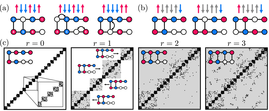
Figure 1: A system with $L=8$ sites, $N=6$ particles and total spin $S^{z}=0$. (a) Illustration of two types of particle hops. The hops within ladder legs do not modify the spin pattern, as shown in the middle sketch. The hops between ladder legs modify the spin pattern, as demonstrated in the right sketch. (b) Illustration of SLIOMs. The particles at the edges of the ladder legs have fixed spins, as they cannot hop to the opposite leg. Spins of other particles are not fixed and can be flipped, as clear from exemplary configurations presented in the middle and right sketches. They are marked grey in the spin pattern. (c) The variation of the Hamiltonian matrix in the computational basis with the number of rungs $r$. Grey squares mark blocks. For $r=1$, an exemplary state from each block is shown. For $r\geq 2$, there is a single block, but clusters of matrix elements become more interconnected as $r$ increases.

$t$-$J_{z}$ model.–In the following, we study the infinite-interaction limit of the anisotropic Fermi-Hubbard Hamiltonian, i.e., the so-called $t$-$J_{z}$ model [39, 40, 41]. We consider the Hilbert space that incorporates the hard-core constraint, where the on-site basis consists of three states: $0,\uparrow,\downarrow$. In this Hilbert space, the Hamiltonian of the $t$-$J_{z}$ model can be written as

$$H=-t\sum_{i=1}^{L-1}\sum_{\sigma=\uparrow,\downarrow}\left({c}_{i,\sigma}^{\dagger}{c}_{i+1,\sigma}+\text{H.c.}\right)+J_{z}\sum_{i=1}^{L-1}S_{i}^{z}S_{i+1}^{z},$$ (1)

where $L$ denotes the number of lattice sites, ${c}^{\dagger}_{i,\sigma}$ (${c}_{i,\sigma}$) creates (annihilates) a fermion with spin $\sigma$ at site $i$, while $S_{i}^{z}=1/2({c}_{i,\uparrow}^{\dagger},{c}_{i,\downarrow}^{\dagger})\sigma^{z}({c}_{i,\uparrow},{c}_{i,\downarrow})^{T}$ is the spin operator with $\sigma_{z}$ corresponding to the Pauli matrix. This Hamiltonian conserves the total particle number, $N=N_{\uparrow}+N_{\downarrow}$, as well as the total spin projection, $S^{z}=\frac{1}{2}(N_{\uparrow}-N_{\downarrow})$, where $N_{\sigma}=\sum_{i=1}^{L}{c}_{i,\sigma}^{\dagger}{c}_{i,\sigma}$. For simplicity, we restrict considerations to a single symmetry sector with a defined $N$ and $S^{z}$. Its dimension is given by $Z=\binom{L}{N}\binom{N}{N_{\sigma}}$.

A hallmark of the $t$-$J_{z}$ model is its kinetically constrained dynamics, which consists of the reordering of $N_{h}=L-N$ holes so that the overall spin pattern remains frozen. As a result, the Hamiltonian exhibits the Hilbert space fragmentation [37], and decomposes into disconnected blocks in the computational basis. There are $B=\binom{N}{N_{\sigma}}$ such blocks, each of dimension $\tilde{Z}=\binom{L}{N}$.

We recall that in integrable systems, configurations of eigenvalues of LIOMs uniquely label all energy eigenstates [42]. In a similar spirit, it has been proposed that in fragmented systems, configurations of eigenvalues of SLIOMs uniquely determine all blocks [37, 38]. For the $t$-$J_{z}$ model, these SLIOMs have already been established, and each of them corresponds to the spin of the $k$th particle with $k\leq N$. It is worth emphasizing that they are not local in the operator sense, i.e., they cannot be written as sums of operators with a finite support over the lattice. Nevertheless, they are local in the statistical sense: the $k$th particle can move through the lattice, but its motion is restricted by the number of holes. Therefore, for typical computational basis states, this particle can be found in the vicinity of the $kL/N$ site [37]. We highlight that the knowledge of SLIOMs is sufficient to characterize the dynamics of a fragmented system, for example, by providing a tight Mazur bound [37, 38].

Tunable Hilbert space fragmentation.–We now demonstrate that it is possible to tune the fragmentation by progressively reducing the number of SLIOMs and, consequently, the number of blocks. This can be achieved in two steps and requires $N_{h}\ll N$. First, we deform the chain with $L$ sites, forming a two-leg ladder with $L/2$ sites coupled by a single rung between positions $i=L/2$ and $j=L/2+1$ (see Fig. 1). Site and particle indices are assigned starting from the rightmost position in the upper leg of the ladder. Next, we progressively add additional $r$ rungs between positions $i=L/2-l$ and $j=L/2+1+l$ with $l=1,...,r$. Explicitly, each additional rung corresponds to $h(l)=-t(l)\sum_{\sigma=\uparrow,\downarrow}({c}_{i,\sigma}^{\dagger}{c}_{j,\sigma}+\text{H.c.})+J_{z}(l)S_{i}^{z}S_{j}^{z}$, where both $t(l)$ and $J_{z}(l)$ can depend on the rung index, $l$. Let us consider the following scenario: a particle reaches a position $i$ in the lower leg that is connected by a rung to the upper leg, see the left panel of Fig. 1(a). If there is a hole in the upper leg, the particle can hop and modify the spin sequence, as illustrated in the right panel of Fig. 1(a). Therefore, the particles that can hop both along the legs and across the rungs behave effectively as in a two-dimensional lattice. In contrast, the particles located far from rungs, i.e., those that either cannot reach any rung or can reach only the last rung when no holes are present in the opposite leg, remain effectively one-dimensional. Their dynamics do not affect the spin pattern, and their spin projection is conserved. As a result, they continue to generate SLIOMs.

The number of SLIOMS in the above setup can be estimated as follows. Consider separating holes by moving them to the rightmost positions in the lower leg, see the left panel of Fig. 1(b). This reveals that there are exactly $N-L/2-r=L/2-N_{h}-r$ particles in the lower leg that have fixed spins. This reasoning can be reversed, yielding the same number of particles in the upper leg. Therefore, the total number of SLIOMs is given by $Q=L-2N_{h}-2r$. If $Q\leq N_{\sigma}$ for both $\sigma$, SLIOMs may have arbitrary spin projections, and the number of blocks can be calculated as $B=\sum_{n=0}^{Q}\binom{Q}{n}=2^{Q}$. Otherwise, if $Q>N_{\sigma}$ for at least one $\sigma$, certain spin configurations are inaccessible and one should adjust the range of summation. Then, the general expression for the number of blocks reads

$$B=\sum_{n=\text{max}[0,Q-N_{-\tilde{\sigma}}]}^{\text{min}[Q,N_{\tilde{\sigma}}]}\binom{Q}{n},$$ (2)

where $\tilde{\sigma}$ is the spin projection of the minority species. Simultaneously, the dimension of a single block depends on the number of SLIOMs that have a spin projection $\tilde{\sigma}$, which is denoted by $n$. This dimension can be determined by counting all possible ways to distribute $N$ particles across $L$ sites and to distribute $N_{\tilde{\sigma}}-n$ minority spins across $N-Q$ effectively two-dimensional particles, i.e., $\tilde{Z}=\binom{L}{N}\binom{N-Q}{{N}_{\tilde{\sigma}}-n}$.

In integrable systems, a perturbation or a change in lattice dimensionality destroys (almost) all LIOMs. In contrast, the system considered above exhibits, to the best of our knowledge, the only known example of tunable Hilbert space fragmentation. Specifically, it allows controlling the number of conservation laws, as adding a single rung to a ladder with $r>0$ breaks exactly two SLIOMs. Our numerical calculations did not reveal any additional blocks $B$ beyond those introduced in Eq. (2). In Fig. 1(c), we illustrate the described behavior: adding one rung to a ladder with $L=8$, $N=6$ and $r=0$ reduces the number of blocks from $20$ to $4$, and adding another rung reduces it further from $4$ to $1$. Additional examples illustrating the tunability of fragmentation are provided in [43].

We now confirm that the number of SLIOMs is reflected in the spin dynamics with direct numerical calculations. We consider a ladder with $t=J_{z}=1$ and $L=16$, fixing $N=13$ and $S^{z}=1/2$. For the additional $r$ rungs, we also set $t(l)=J_{z}(l)=1$. As the initial state, we choose the computational basis state $|\psi_{0}\rangle=\left|\uparrow\dots\uparrow 0\dots 0\downarrow\dots\downarrow\rangle\right.$, where all spin-up (spin-down) particles occupy the rightmost positions in the upper (lower) leg. The state at finite times, $|\psi_{t}\rangle$, is obtained using the Lanczos propagation method [44, 45]. Finally, we compute the expectation values of spin projections, $\langle\psi_{t}|S^{z}_{i}|\psi_{t}\rangle$, for all sites $i\leq L$.

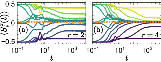
Figure 2: The time evolution of spin projections, $\langle\psi_{t}|S^{z}_{i}|\psi_{t}\rangle$, for all sites $i\leq L$. We focus on a system with $L=16$ sites, $N=13$ particles, and total spin $S^{z}=1/2$. Results in (a) and (b) were calculated for $r=2$ ($Q=6$) and $r=4$ ($Q=2$), respectively. The initial state was the computational basis state with spin-up (spin-down) particles occupying the rightmost positions in the upper (lower) leg. The dashed lines mark the thermal prediction $(N_{\uparrow}-N_{\downarrow})/(2L)\approx 0.031$.

Results for a ladder with $r=2$ ($Q=6$) and $r=4$ ($Q=2$) are presented in panels (a) and (b) of Fig. 2, respectively. Changing the number of SLIOMs clearly modifies the expectation values $\langle\psi_{t}|S^{z}_{i}|\psi_{t}\rangle$. This conclusion is nontrivial, as nonlocal conservation laws typically do not affect the time evolution of local operators [46]. It agrees with a recent observation that SLIOMs can give rise to a tight Mazur bound [37, 38], and it facilitates the study in the next section, where we treat SLIOMs in a similar spirit to LIOMs. We also highlight an exceptionally broad range of relaxation times of $\langle\psi_{t}|S^{z}_{i}|\psi_{t}\rangle$, a feature that is difficult to realize in integrable or nearly integrable models [47, 48, 49]. In general, $S^{z}_{i}$ closer to the ladder edges exhibit larger projections onto SLIOMs and evolve more slowly. Some of these spins do not relax to the thermal prediction, although they are not strictly conserved.

Extended critical regime–Many measures are sensitive to the breaking of integrability and can therefore be used to detect the transition to the ergodic regime. By far, the most commonly studied ones are the spectral statistics [50, 51, 52, 53, 54], entanglement entropy [55, 56, 57, 58, 59] and (recently) fidelity susceptibility [20, 21, 22, 23, 24, 25, 26]. Most of these measures are essentially binary in nature. For example, the spectral statistics can either follow Wigner-Dyson or Poisson distribution, while the entanglement entropy can either be maximal or not. Surprisingly, we now demonstrate that, in our ladder with tunable fragmentation, the fidelity susceptibility can reveal the breaking of only a few conservation laws, thereby identifying the transition between two nonergodic regimes.

The fidelity susceptibility of a single energy eigenstate, $H(\lambda)|n(\lambda)\rangle=E_{n}(\lambda)|n(\lambda)\rangle$, quantifies the sensitivity of this state to changes in the Hamiltonian, $\partial_{\lambda}H$. Its average over all energy eigenstates, $|n(\lambda)\rangle$, is given by [60, 61, 5]

$$\chi_{\text{av}}=\frac{1}{Z}\sum_{n=1}^{Z}\sum_{m\neq n}\frac{\omega_{nm}^{2}}{(\omega_{nm}^{2}+\mu^{2})^{2}}\left|\langle n(\lambda)|\partial_{\lambda}H|m(\lambda)\rangle\right|^{2},$$ (3)

where we defined $\omega_{nm}=E_{n}(\lambda)-E_{m}(\lambda)$. From now on, we focus on the limit $\lambda\rightarrow 0$ and make the dependence on $\lambda$ implicit. In Eq. (3), we introduced the energy cutoff $\mu$, which is known as regularization [5]. Usually, $\omega_{H}<\mu\ll\Delta E$, where $\omega_{H}\propto 1/Z$ is the Heisenberg energy (the mean level spacing, serving as the minimal relevant energy scale in a finite system) and $\Delta E\propto L$ is the energy bandwidth. The role of $\mu$ is twofold. Firstly, it removes the issue of an ill-defined denominator in Eq. (3) for degenerate energy eigenstates. However, its true importance is revealed when the average fidelity susceptibility, $\chi_{\text{av}}$, is rewritten as [62]

$$\chi_{\text{av}}\mu\propto|f(\omega\approx\mu)|^{2},$$ (4)

where the spectral function, $|f(\omega)|^{2}$, is the Fourier transform of the autocorrelation function of $\partial_{\lambda}H$,

$$|f(\omega)|^{2}=\frac{1}{2\pi Z}\sum_{n=1}^{Z}\int_{-\infty}^{\infty}dte^{i\omega t}\langle n|\partial_{\lambda}H(t)\partial_{\lambda}H|n\rangle_{c},$$ (5)

and $\langle n|O(t)O|n\rangle_{c}=\langle n|O(t)O|n\rangle-\langle n|O(t)|n\rangle\langle n|O|n\rangle$. The derivation of the relation from Eq. (4) can be found in [43]. Thus, studying the rescaled fidelity susceptibility, $\chi_{\text{av}}\mu$, for different energy cutoffs, $\mu$, amounts to probing the system dynamics at different times, $t\approx\mu^{-1}$. When the autocorrelation function of $\partial_{\lambda}H$ decays exponentially with the relaxation time $\tau$, the spectral function from Eq. (5) is a Lorentzian, whose maximum value is proportional to $\tau$. Therefore, for small energy cutoffs, $\mu\approx\omega_{H}$, the rescaled fidelity susceptibility, $\chi_{\text{av}}\mu$, provides a rough estimate of the relaxation time, $\tau$.

In ergodic systems, the spectral function $|f(\omega)|^{2}$ is related to the envelope function from the ETH ansatz and forms a plateau for low $\omega$ [63]. This plateau indicates when the ETH ansatz becomes equivalent to the RMT ansatz in the frequency domain or, equivalently, when the perturbation $\partial_{\lambda}H$ relaxes in the time domain. Consequently, $\chi_{\text{av}}\mu$ is independent of $\mu^{-1}$, as obvious from Eq. (4). In integrable systems, the spectral weight accumulates at $\omega=0$, forming a Drude-like peak, and the spectral function $|f(\omega)|^{2}$ develops a gap at low $\omega\neq 0$ [64, 65, 66]. This behavior can be related to the existence of LIOMS [46, 67] and results in $\chi_{\text{av}}\mu$ decreasing with $\mu^{-1}$ [6, 62]. Near the ergodicity-breaking transition, the spectral function $|f(\omega)|^{2}$ usually develops a polynomially decaying tail that can span several orders of magnitude in $\omega$ [6, 62]. Such behavior indicates that LIOMs acquire finite relaxation times, leading to the broadening of a Drude-like peak [67]. As a result, $\chi_{\text{av}}\mu\propto\mu^{-\alpha}$ with $\alpha\in(0,1]$. It exhibits a maximum pinned to the critical point, indicating the exceptionally slow relaxation of the perturbation $\partial_{\lambda}H$ [27, 28, 29] - the phenomenon which is known as maximal chaos.

We design the following experiment using the ladders described above with $t=J_{z}=1$. We treat $r$ as a continuous parameter, where its integer part determines the number of additional rungs with the same coupling strength, i.e., $t(l)=J_{z}(l)=1$ for $l=1,\dots,[r]$. Simultaneously, its fractional part sets the coupling strength of the last rung, i.e., $t(l)=J_{z}(l)=\left\{r\right\}$ for $l=[r]+1$. This allows for the possibility of weakly broken SLIOMs for small but nonzero $\left\{r\right\}$, resembling weakly broken LIOMs in nearly integrable systems. We focus on the perturbation in the form of the next-nearest neighbor hopping, $\partial_{\lambda}H=\frac{1}{\sqrt{L}}\sum_{\sigma=\uparrow,\downarrow}\sum_{i=1}^{L-2}(c_{i,\sigma}^{\dagger}c_{i+2,\sigma}+\text{H.c.})$, which is local and does not share the block structure of the Hamiltonian. The coefficient in front of the sum ensures the unit Hilbert-Schmidt norm, see the discussion in [68]. Moreover, we focus on the middle of the spectrum, so that we average the rescaled fidelity susceptibility over a fraction of all energy eigenstates. See [43] for technical details and additional perturbations. Finally, we tune $r$ and determine if $\chi_{\text{av}}\mu$ develops maxima for vanishing $\left\{r\right\}$.

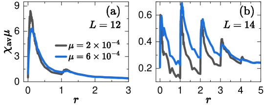
Figure 3: Rescaled fidelity susceptibilities $\chi_{\text{av}}\mu$ plotted against rung number $r$ for a ladder with (a) $L=12$ sites, $N=8$ particles and total spin $S^{z}=0$. Analogical results, but for a ladder with $L=14$ sites, $N=12$ particles, and total spin $S^{z}=0$, are presented in (b). We consider two energy cutoffs, $\mu=2\times 10^{-4}$ and $6\times 10^{-4}$.

In panels (a) and (b) of Fig. 3, we show the evolution of the rescaled fidelity susceptibility, $\chi_{\text{av}}\mu$, with the number of rungs, $r$, for a ladder with $L=12\,,N=8,S^{z}=0$ and $L=14\,,N=12,S^{z}=0$, respectively. For both ladders and energy cutoffs considered, $\chi_{\text{av}}\mu$ develops pronounced peaks, which signal an ultra-slow relaxation of $\partial_{\lambda}H$, near all transitions that separate regimes with different numbers of SLIOMs. This behavior is nontrivial, as it demonstrates that $\chi_{\text{av}}\mu$, unlike other standard ergodicity indicators, is sensitive to the breaking of as few as two SLIOMs. In [43], we also confirm that $\chi_{\text{av}}\mu$ increases with $\mu^{-1}$ near transitions (for $\left\{r\right\}\approx 0$), while it decreases with $\mu^{-1}$ away from transitions (for $\left\{r\right\}\gg 0$). Consequently, the critical regime extends over $0\leq r\leq r^{\prime}$ and exhibits $r^{\prime}+1$ peaks, where fragmentation disappears at $r^{\prime}=L/2-N_{h}$. The number of such peaks increases with the system size, since more rungs can be added before all SLIOMs are broken. This is remarkable, as conventional integrability-breaking transitions, like the one induced by adding the next-nearest-neighbor hopping to the Heisenberg XXZ chain [27], feature a single peak. The existence of an extended critical regime with multiple peaks of $\chi_{\text{av}}\mu$ is one of the most important outcomes of our study.

Conclusions–In this letter, we have introduced a protocol that enables tuning of the Hilbert-space fragmentation in the $t$–$J_{z}$ model. Specifically, by progressively including hopping terms, more particles become effectively two-dimensional, resulting in the successive breaking of conservation laws (SLIOMs). We have derived closed-form expressions for the numbers of SLIOMs and blocks. We have also performed direct numerical calculations, demonstrating that the existence of SLIOMs is reflected in spin dynamics, leading to an exceptionally broad range of relaxation times, a feature difficult to realize in integrable or nearly integrable models.

Finally, we have also studied the behavior of the rescaled fidelity susceptibility, which measures the sensitivity of energy eigenstates to modifications of the Hamiltonian. We have found that our model with tunable Hilbert-space fragmentation supports an extended critical regime, where the rescaled fidelity susceptibility exhibits multiple maxima. Each maximum signals a change in the number of SLIOMs, as well as an ultra-slow relaxation of local observables. Moreover, the number of maxima increases with the number of lattice sites. We emphasize that this is a highly nontrivial behavior, as typical integrability-breaking transitions feature a single peak signaling the breaking of all LIOMs.

a

S1 Examples of tunable Hilbert space fragmentation.

In Tab. S1, we show how the Hilbert-space fragmentation can be tuned by increasing the number of additional rungs $r$.

$r$	0	1	2	3	4	5
$B\,(L=12)$	70	4	1	1	1	1
$B\,(L=14)$	924	256	64	16	4	1
$B\,(L=16)$	8192	256	64	16	4	1

Table S1: The number of blocks, $B$, versus the number of additional rungs, $r$, for different ladders with $L$ sites, $N_{h}$ holes, and total spin $S^{z}$. We consider $L=12$ with $N_{h}=4$ and $L=14$ with $N_{h}=2$. Both ladders have $S^{z}=0$. Additionally, we include $L=16$ with $N_{h}=3$ and $S^{z}=1/2$.

S2 Derivation of Eq. (4).

The fidelity susceptibility naturally arises when considering the sensitivity of a system to changes in the Hamiltonian. For example, let us consider

$$H(\lambda)=H_{0}+\lambda O,$$ (S1)

and we refer to $\partial_{\lambda}H=O$ as a perturbation. The modification of energy eigenstates, $H(\lambda)|n(\lambda)\rangle=E(\lambda)|n(\lambda)\rangle$, can be quantified by the following overlap (up to the second order in $d\lambda$) [60]

$$|\langle n(\lambda)|n(\lambda+d\lambda)\rangle|^{2}\approx 1-\chi_{n}d\lambda^{2},$$ (S2)

where the coefficient $\chi_{n}$ is known as the fidelity susceptibility and is given by

$$\chi_{n}=\sum_{m\neq n}\frac{|\langle n(\lambda)|O|m(\lambda)\rangle|^{2}}{\omega_{nm}^{2}}.$$ (S3)

In the above equation, we defined $\omega_{nm}=E_{n}(\lambda)-E_{m}(\lambda)$. From now on, we focus on the limit $\lambda\rightarrow 0$ and we make the dependence on $\lambda$ implicit.

Intuitively, ergodic systems are expected to be chaotic and more sensitive to perturbations than integrable ones. Therefore, the fidelity susceptibility, when averaged over all energy eigenstates, can serve as an indicator of the integrability-breaking transitions [5]. To avoid an ill-defined denominator for degenerate energy eigenstates, and to probe the system’s dynamics at a selected energy scale $\mu$ (or at selected timescale $\tau=\mu^{-1}$), we consider its regularized version

$$\chi_{\text{av}}=\frac{1}{Z}\sum_{n=1}^{Z}\sum_{m\neq n}\frac{\omega_{nm}^{2}}{(\omega_{nm}^{2}+\mu^{2})^{2}}|\langle n|O|m\rangle|^{2},$$ (S4)

where $Z$ is the Hilbert space dimension (in the given symmetry sector). The energy cutoff is usually restricted to $\omega_{H}<\mu\ll\Delta E$, where $\omega_{H}\propto Z^{-1}$ is the Heisenberg energy and $\Delta E$ is the energy bandwidth. To simplify the expression from Eq. (S4), we replace the sums with integrals and perform the substitution of variables, i.e., $E_{n}=E+\omega/2$ and $E_{m}=E-\omega/2$. We arrive at

$$\chi_{\text{av}}=\frac{1}{Z}\int\limits_{-\infty}^{\infty}\int\limits_{-\infty}^{\infty}\mspace{-3.0mu}dEd\omega\mspace{2.0mu}\rho\mspace{-4.0mu}\left(E+\frac{\omega}{2}\right)\rho\mspace{-4.0mu}\left(E-\frac{\omega}{2}\right)\frac{\omega^{2}|\langle n|O|m\rangle|^{2}}{(\omega^{2}+\mu^{2})^{2}},$$ (S5)

where $\rho(E)\propto Z$ is the density of states. Taking into account that

• offdiagonal matrix elements, both in ergodic [69, 70] and integrable [64, 65, 66] systems, can be approximated as $|\langle n|O|m\rangle|^{2}\approx\rho(E)^{-1}|f(E,\omega)|^{2}$, where $f(E,\omega)$ is a smooth function of its arguments,

• $\Delta(\omega)=(2\mu/\pi)/[\omega^{2}/(\omega^{2}+\mu^{2})^{2}]$ is a probability distribution function sharply peaked at $\omega=\mu$,

• $\rho(E\pm\mu/2)\approx\rho(E)$,

we establish the relation from the main text:

$$\chi_{\text{av}}\mu\propto\frac{1}{Z}\int\limits_{-\infty}^{\infty}\mspace{-3.0mu}dE\rho(E)|f(E,\mu)|^{2}=|f(\mu)|^{2}.$$ (S6)

Finally, we highlight that the average over mean energies, $|f(\omega)|^{2}$, corresponds to the spectral function, which is the Fourier transform of the autocorrelation function,

$$|f(\omega)|^{2}=(2\pi Z)^{-1}\sum_{n=1}^{Z}\int\limits_{-\infty}^{\infty}dte^{i\omega t}[\langle n|O(t)O|n\rangle-|\langle n|O|n\rangle|^{2}]\,.$$ (S7)

S3 Details of numerical calculations.

Fidelity susceptibilities, $\chi_{\text{av}}$, were calculated as

$$\chi_{\text{av}}=\frac{1}{D}\sum_{n=1}^{D}\sum_{\begin{subarray}{c}m=1,\\ m\neq n\end{subarray}}^{Z}\frac{\omega_{nm}^{2}}{(\omega_{nm}^{2}+\mu^{2})^{2}}\left|\langle n|\partial_{\lambda}H|m\rangle\right|^{2},$$ (S8)

where $Z$ is the Hilbert space dimension (in the given symmetry sector). For the systems with $L=12,N=8,S^{z}=0$, the averaging was performed over $D=800$ energy eigenstates from the middle of the spectrum. For $L=14,N=12,S^{z}=0$, the averaging was performed over $D=4000$ ($D=800$) energy eigenstates from the middle of the spectrum when $r\leq 3$ ($r>3$).

According to Eq. (4) from the main text, the behavior of the fidelity susceptibility, $\chi_{\text{av}}$, is encoded in the spectral function, $|f(\omega)|^{2}$. The latter function can be calculated from coarse-grained offdiagonal matrix elements:

$$|f(\omega)|^{2}\approx\frac{Z}{D}\sum_{\begin{subarray}{c}n,m\neq n\\ |(E_{n}+E_{m})/2|<\Delta E\\ |(E_{n}-E_{m})-\omega|<\Delta\omega\end{subarray}}|\langle n|\partial_{\lambda}H|m\rangle|^{2},$$ (S9)

where $Z$ is the Hilbert space dimension (in the given symmetry sector), $\Delta E=0.025L$ and $\Delta\omega$ was established by dividing the range $\log_{10}(\omega_{H})<\log_{10}(\omega)<0$ into $160$ bins, where $\omega_{H}\approx 10^{-4}$ is the Heisenberg energy. Additionally, $D$ is the number of offdiagonal matrix elements that satisfy the conditions $|(E_{n}+E_{m})/2|<\Delta E$ and $|(E_{n}-E_{m})-\omega|<\Delta\omega$. In the final step, we applied a moving average over $20$ bins to smooth out the oscillations visible in the low-$\omega$ regime.

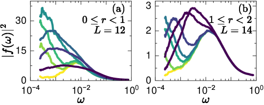
Figure S1: (a) Spectral functions $|f(\omega)|^{2}$ shown for a ladder with $L=12$ near the eigenstate transition at $r=0$, i.e., $r=0$, $0.01$, $0.02$, $0.05$, $0.2$, $0.3$ and $0.6$. (b) Same results for $L=14$ and $r=1$, i.e., $r=1$, $1.004$, $1.01$, $1.015$, $1.03$, $1.1$ and $1.2$. Darker colors indicate larger $r$.

We now show how the spectral function $|f(\omega)|^{2}$ evolves with $r$ for the perturbation studied in the main text, i.e., $\partial_{\lambda}H=\frac{1}{\sqrt{L}}\sum_{\sigma=\uparrow,\downarrow}\sum_{i=1}^{L-2}(c_{i,\sigma}^{\dagger}c_{i+2,\sigma}+\text{H.c.})$. In panels (a) and (b) of Fig. S1, we present results for a ladder with $L=12,N=8,S^{z}=0$ near $r=0$ and $L=14,N=12,S^{z}=0$ near $r=1$, respectively. Darker colors indicate larger $\left\{r\right\}$. We observe that for $\left\{r\right\}\approx 0$, the spectral function $|f(\omega)|^{2}$ exhibits a gap, which is characteristic of integrable systems and has been related to the existence of LIOMs. In the fragmented system considered here, this feature is most likely associated with the presence of SLIOMs. As $\left\{r\right\}$ increases, $|f(\omega)|^{2}$ develops a polynomial tail, indicating an exceptionally slow relaxation of the autocorrelation function of $\partial_{\lambda}H$. This results from the breaking of a subset of SLIOMs. Eventually, as the relaxation times of the former SLIOMs decrease and become much shorter than the Heisenberg time $\tau_{H}=\omega_{H}^{-1}$, the polynomial tail of $|f(\omega)|^{2}$ shifts to higher $\omega$, revealing a gap associated with the remaining SLIOMs.

We emphasize that when calculating $|f(\omega)|^{2}$ and $\chi_{\text{av}}$, we add the term $0.5n_{L,\uparrow}+n_{L,\downarrow}$ to the Hamiltonian to break the parity and spin-inversion symmetries. It does not affect the Hilbert-space fragmentation and becomes relevant only in the ergodic regime, where the Hamiltonian comprises a single block.

S4 $\chi_{\text{av}}\mu$ and $|f(\omega)|^{2}$ for different $\partial_{\lambda}H$.

In the main part of this manuscript, we considered the next-nearest neighbor hopping as a perturbation, i.e., $\partial_{\lambda}H=\frac{1}{\sqrt{L}}\sum_{\sigma=\uparrow,\downarrow}\sum_{i=1}^{L-2}(c_{i,\sigma}^{\dagger}c_{i+2,\sigma}+\text{H.c.})$. This choice was motivated by its locality and the presence of nonzero matrix elements between states from different blocks. It ensures that the behavior of the rescaled fidelity susceptibility, $\chi_{\text{av}}\mu$, and the spectral function, $|f(\omega)|^{2}$, is not a trivial consequence of $\partial_{\lambda}H$ sharing the block structure with $H$ at $\lambda=0$. Here, we extend the study to two additional perturbations. Particularly, the site occupation in the middle of the ladder,

$$\partial_{\lambda}H=n_{L/2}=\sum_{\sigma=\uparrow,\downarrow}c_{L/2,\sigma}^{\dagger}c_{L/2,\sigma},$$ (S10)

which is local and diagonal in the computational basis, and the occupation of the zero-momentum mode,

$$\partial_{\lambda}H=m_{0}=\sum_{\sigma=\uparrow,\downarrow}\sum_{i,j=1}^{L}c_{i,\sigma}^{\dagger}c_{j,\sigma},$$ (S11)

which is nonlocal (but few-body) and couples states from different blocks.

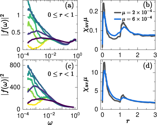
Figure S2: Numerical results for a ladder with $L=12$. Spectral functions $|f(\omega)|^{2}$ near the eigenstate transition at $r=0$ for (a) $n_{L/2}$ and (c) $m_{0}$. We consider $r=0$, $0.01$, $0.02$, $0.05$, $0.1$, $0.25$, $0.6$ and darker colors indicate larger $r$. Rescaled fidelity susceptibilities $\chi_{\text{av}}\mu$ plotted against $r$ for (b) $n_{L/2}$ and (d) $m_{0}$. We consider $\mu=2\times 10^{-4}$ and $6\times 10^{-4}$.

Results of numerical calculations for a ladder with $L=12,N=8,S^{z}=0$ are shown in Fig. S2. The spectral functions $|f(\omega)|^{2}$ near the eigenstate transition at $r=0$ are presented in panels (a) and (c) for the site occupation $n_{L/2}$ and the momentum mode occupation $m_{0}$, respectively. Darker colors indicate larger $r$. Additionally, the rescaled fidelity susceptibilities $\chi_{\text{av}}\mu$ are plotted against $r$ in panel (b) for $n_{L/2}$ and in panel (d) for $m_{0}$. We consider $\mu=2\times 10^{-4}$ and $6\times 10^{-4}$. Results of numerical calculations for a system with $L=14,N=12,S^{z}=0$ are shown in Fig. S3. Focusing on $n_{L/2}$, the spectral functions $|f(\omega)|^{2}$ near the eigenstate transition at $r=1$ are depicted in panel (a), while the rescaled fidelity susceptibility $\chi_{\text{av}}\mu$ is plotted against $r$ in panel (b). Clearly, $|f(\omega)|^{2}$ and $\chi_{\text{av}}\mu$ exhibit qualitatively similar behavior for all considered perturbations.

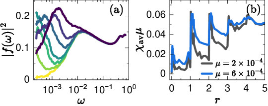
Figure S3: Numerical results for a ladder with $L=14$. We focus on the perturbation $n_{L/2}$. (a) Spectral functions $|f(\omega)|^{2}$ near the eigenstate transition at $r=1$. We consider $r=1$, $1.004$, $1.01$, $1.015$, $1.03$, $1.05$, $1.1$ and darker colors indicate larger $r$. (b) Rescaled fidelity susceptibilities $\chi_{\text{av}}\mu$ plotted against $r$. We consider $\mu=2\times 10^{-4}$ and $6\times 10^{-4}$.

We complement the analysis by showing that the eigenstate transitions can also be inferred from the distributions of offdiagonal matrix elements. Deep in the ergodic regime, these distributions are expected to be Gaussian, at least for energy eigenstates with close energies [71, 65, 64]. Therefore, we consider the measure [57],

$$\Gamma=\frac{\overline{|\langle n|\partial_{\lambda}H|m\rangle|^{2}}}{\overline{|\langle n|\partial_{\lambda}H|m\rangle|}^{2}}$$ (S12)

with

$$\overline{f(\langle n|O|m\rangle)}=\sum_{\begin{subarray}{c}n,m\neq n\\ |(E_{n}+E_{m})/2|<0.025L\\ |E_{n}-E_{m}|<0.02\end{subarray}}f(\langle n|O|m\rangle),$$ (S13)

which equals $\pi/2$ for a Gaussian distribution.

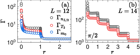
Figure S4: The measure $\Gamma$ plotted against $r$ for a ladder with (a) $L=12$ and (b) $L=14$. We consider three perturbations, i.e., the next-nearest neighbor hopping $T_{2}$, the site occupation $n_{L/2}$, and the zero momentum mode occupation $m_{0}$ (for $L=12$). The horizontal lines mark the expectation for the Gaussian distribution, i.e., $\Gamma=\pi/2$.

In Fig. S4, we present $\Gamma$ as functions of $r$ for all considered $\partial_{\lambda}H$. Results for ladders with $L=12,N=8,S^{z}=0$ and $L=14,N=12,S^{z}=0$ are shown in panels (a) and (b), respectively. We first note that, in agreement with expectations, $\Gamma\approx\pi/2$ when the Hamiltonian consists of a single block. This occurs for $r>1$ when $L=12$ and for $r>4$ when $L=14$. Moreover, $\Gamma$ exhibits a jump near each eigenstate transition and remains approximately constant between the transitions. This behavior is the most easily explained for the site occupation, $\partial_{\lambda}H=n_{L/2}$, as it is diagonal in the computational basis. Since its offdiagonal matrix elements between energy eigenstates from different blocks are exactly zero, their number increases with decreasing $r$, leading to the emergence of a singularity in the distribution. Similar behavior has been observed for local observables when the system approaches the integrable point, i.e., the distribution of offdiagonal matrix elements develops a peak around zero so that it can be modeled as a combination of two Gaussians [72].

S5 Scaling of the maxima of $\chi_{\text{av}}$.

In this section, we study the behavior of $\chi_{\text{av}}$ with $\mu^{-1}$ in detail. We recall that $\chi_{\text{av}}$ is expected to scale as $\mu^{-\alpha}$ with $\alpha\in(1,2]$ in the vicinity of its maxima [6, 62]. (Note that in the main text, we study $\chi_{\text{av}}\mu$ instead of $\chi_{\text{av}}$, so that $\alpha\in(0,1]$ rather than $(1,2]$.) Simultaneously, it scales as $\mu^{-1}$ in ergodic systems, while it increases more slowly than polynomially in integrable and generally nonergodic systems.

In Figs. S5(a) and S5(b), we plot $\chi_{\text{av}}$ against $\mu^{-1}$ for selected $r$. We focus on the perturbation from the main text, i.e., $\partial_{\lambda}H=\frac{1}{\sqrt{L}}\sum_{\sigma=\uparrow,\downarrow}\sum_{i=1}^{L-2}(c_{i,\sigma}^{\dagger}c_{i+2,\sigma}+\text{H.c.})$, and we consider a ladder with $L=12,N=8,S^{z}=0$. As indicated in panel (a) by circles an upward triangles, the behavior of the fidelity susceptibility near the eigenstate transitions is consistent with the scaling $\mu^{-\alpha}$ with $\alpha\in(1,2]$. As indicated in the same panel by downward triangles, $\chi_{\text{av}}$ in the non-fragmented system closely follows $\mu^{-1}$. Finally, the fidelity susceptibility calculated in the fragmented system far from eigenstate transitions shows bending in the log-log scale, suggesting that $\chi_{\text{av}}$ increases more slowly than polynomially with $\mu^{-1}$, see panel (b). The curves from Figs. S5(a) and S5(b) correspond to the highlighted points in Fig. S5(c).

We complement the study with the calculation of

$$\gamma=\frac{\partial\log_{10}\chi_{\text{av}}}{\partial\log_{10}\mu^{-1}}.$$ (S14)

Numerically, $\gamma$ is determined by calculating four two-point derivatives in the range $\mu\in[2\times 10^{-4},12\times 10^{-4}]$ and averaging the results. We note that if $\chi_{\text{av}}\propto\mu^{-\alpha}$ then $\gamma=\alpha$. In Figs. S5(c) and S5(d), we plot $\gamma$ against $r$ for a ladders with $L=12,N=8,S^{z}=0$ and $L=14,N=12,S^{z}=0$, respectively. The solid lines mark the prediction for ergodic systems, i.e., $\gamma=1$. In agreement with previous findings, we observe $\gamma<1$ for fragmented systems, $\gamma=1$ for non-fragmented systems, and $\gamma>1$ near eigenstate transitions.

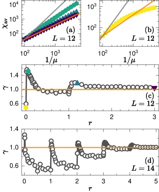
Figure S5: (a,b) The fidelity susceptibility $\chi_{\text{av}}$ plotted against the inverse of energy cutoff $\mu^{-1}$ for a ladder with $L=12$. In panel (a), we consider $r=0.05$ (circles), $1.2$ (upward triangles), $3$ (downward triangles). In panel (b), we consider $r=0$ (squares). Two solid lines mark the limiting predictions, i.e., $\chi_{\text{av}}\propto\mu^{-1}$ and $\chi_{\text{av}}\propto\mu^{-2}$. The curves from panels (a) and (b) correspond to the highlighted points from panel (c). The derivative $\gamma$ as a function of $r$ for a ladder with (c) $L=12$ and (d) $L=14$. The solid lines mark the prediction for ergodic systems, i.e., $\gamma=1$.