A Thermodynamic Framework for Coherently Driven Systems

Abstract

The laws of thermodynamics are a cornerstone of physics. At the nanoscale, where fluctuations and quantum effects matter, there is no unique thermodynamic framework because thermodynamic quantities such as heat and work depend on the accessibility of the degrees of freedom. We derive a thermodynamic framework for coherently driven systems, where the output light is assumed to be accessible. The resulting second law of thermodynamics is strictly tighter than the conventional one and it demands the output light to be more noisy than the input light. We illustrate our framework across several well-established models and we show how the three-level maser can be understood as an engine that reduces the noise of a coherent drive. Our framework opens a new avenue for investigating the noise properties of driven-dissipative quantum systems.

Introduction – In the last decades the laws of thermodynamics, traditionally used to describe macroscopic systems, have been extended to small, stochastic systems and even to the quantum regime with great success [1, 2, 3, 4, 5, 6, 7, 8]. A major obstacle in this endeavor turned out to be the definition of one of the most central quantities: work [9, 10, 11, 12]. At the macroscale, work is carried by the accessible, macroscopic degrees of freedom, while heat is carried by the microscopic, inaccessible degrees of freedom. At the nanoscale, all degrees of freedom are microscopic, resulting in ambiguity when defining work. To remedy this situation, definitions for work that depend on the considered task have been suggested [13, 14, 15].

The most prominent definition for work (henceforth called the conventional definition) relies on a semiclassical description in terms of a time-dependent Hamiltonian. Work is then described by the energy changes due to its time-dependence, which are induced by controllable degrees of freedom that are described classically [4, 7, 8]. While often adequate, this approach has conceptual shortcomings for coherently driven systems. To illustrate this, we consider an optical cavity that is driven by coherent light as sketched in Fig. 1. In this scenario, the drive can be described by a time-dependent Hamiltonian and the conventional definition can be applied. However, all the energy that leaks out of the cavity is then treated as heat, even if it contains coherence. This may be appropriate if the light leaving the cavity is dissipated but as pointed out in Ref. [15], this light may be further used. This becomes particularly obvious in the case of an empty cavity, where the light is simply reflected with a shifted phase. The output light leaving the cavity is then just as useful as the input light that induces the time-dependence of the Hamiltonian.

In Ref. [15], a resolution of this issue was suggested by considering the coherent part of the output light as work, not heat. However, it remains unclear if this intuitive definition for work can be embedded in a thermodynamically consistent framework where a nonnegative entropy production is associated to the corresponding definition of heat.

Figure 1: The general scenario. A cavity with an embedded quantum system is driven by the input field, which contains a coherent part, given by $\langle\hat{b}_{\rm in}\rangle$ as well as thermal fluctuations. Compared to the input, the output field typically has a smaller coherent part and larger fluctuations. Work ($P^{\rm io}$) and heat ($J^{\rm io}$) are given by the changes in the coherent part and the fluctuations respectively.

In this Letter, we solve this critical problem by formulating the first and second law of thermodynamics consistent with these new definitions. In this framework, the second law demands that the noise in the output light is larger than the noise in the input light, as long as there is no other source of entropy production. We further show that our new second law is always tighter than the conventional second law. This is consistent with treating the output light as accessible: having more access generally reduces irreversibility. We illustrate our thermodynamic framework with the help of a Kerr oscillator, a two-level system embedded in a cavity, and a three-level maser [13, 16]. The last acts as a heat engine, which in our framework corresponds to a machine that can reduce the noise in the light field.

System and Model – We consider a quantum system placed inside a cavity that is subjected to a coherent drive and couples to a bosonic bath via one channel, see Fig. 1. The Hamiltonian of our system reads

$$\hat{H}(t)=\Omega\hat{a}^{\dagger}\hat{a}+\hat{H^{\prime}}+\hat{H}_{\rm d}(t)~,$$ (1)

where $\hat{H}^{\prime}$ describes the system inside the cavity, as well as its coupling to the cavity mode, and the drive term is given by

$$\hat{H}_{\rm d}(t) =i\sqrt{\kappa}\left(\langle\operatorname{\hat{\textit{b}}_{\text{in}}^{\dagger}}(t)\rangle\hat{a}-\langle\operatorname{\hat{\textit{b}}_{\text{in}}}(t)\rangle\hat{a}^{\dagger}\right)\operatorname{~,}$$ (2)

with $\kappa$ denoting the linewidth of the cavity. We further introduced the input field which describes the coherent drive as well as the thermal noise entering the cavity [17]

$$\langle\operatorname{\hat{\textit{b}}_{\text{in}}}(t)\rangle=f(t)e^{-i\omega_{\rm d}t},\hskip 7.11317pt\langle\!\langle\operatorname{\hat{\textit{b}}_{\text{in}}^{\dagger}}(t)\operatorname{\hat{\textit{b}}_{\text{in}}}(t^{\prime})\rangle\!\rangle=n_{\rm c}\delta(t-t^{\prime}),$$ (3)

where $n_{\rm c}$ denotes the thermal occupation and $\langle\!\langle\hat{A}\hat{B}\rangle\!\rangle=\langle\hat{A}\hat{B}\rangle-\langle\hat{A}\rangle\langle\hat{B}\rangle$. We consider a drive at frequency $\omega_{\rm d}$ with a potential slow modulation, i.e. $|\partial_{t}f(t)|/|f(t)|\ll\omega_{\rm d}$.

We model the dynamics of our system with the quantum master equation

$$\partial_{t}\hat{\rho}(t)=-i\quantity[\hat{H}(t),\hat{\rho}(t)]+\mathcal{L}_{\rm c}\hat{\rho}(t)+\mathcal{L}^{\prime}\hat{\rho}(t)\operatorname{~,}$$ (4)

where $\mathcal{L}^{\prime}$ accounts for dissipation of the intra-cavity system and the dissipator of the cavity mode reads,

$$\mathcal{L}_{\rm c}\hat{\rho} =\kappa n_{\rm c}\mathcal{D}[\hat{a}^{\dagger}]\hat{\rho}+\kappa(n_{\rm c}+1)\mathcal{D}[\hat{a}]\hat{\rho}\operatorname{~,}$$ (5)

with $\mathcal{D}[\hat{a}]\hat{\rho}=\hat{a}\hat{\rho}\hat{a}^{\dagger}-\frac{1}{2}\{\hat{a}^{\dagger}\hat{a},\hat{\rho}\}$. We assume that photons can only be exchanged with the input channel and thus demand that $\Tr{\hat{a}^{\dagger}\hat{a}\mathcal{L}^{\prime}\hat{\rho}}=0$. Additional dissipation channels for the photons can be included, see the supplemental material [18]. To describe the light that is reflected by the cavity, we introduce the output operator [17]

$$\hat{b}_{\text{out}}=\hat{b}_{\text{in}}+\sqrt{\kappa}\hat{a}\operatorname{~.}$$ (6)

Thermodynamics – The first law of thermodynamics states that any change in the internal energy $U$ of a system can be divided into heat and work

$$\partial_{t}U=P+J\operatorname{~,}$$ (7)

where $P$ denotes power (work per unit time) and $J$ the heat current. The second law constrains the physically allowed processes by demanding a nonnegative entropy production defined as

$$\dot{\Sigma}\equiv k_{\rm B}\partial_{t}S_{\rm vN}(\hat{\rho})-\frac{J_{\rm c}}{T_{\rm c}}-\frac{J^{\prime}}{T^{\prime}}\geq 0\operatorname{~,}$$ (8)

with the von Neumann entropy $S_{\text{vN}}(\hat{\rho})=-\Tr{\hat{\rho}\ln\hat{\rho}}$. Here we split the heat current into two parts $J=J_{\rm c}+J^{\prime}$ corresponding to the dissipation of the cavity and the intra-cavity system respectively. The cavity temperature is defined through $n_{\rm c}=[e^{\omega_{d}/(k_{\rm B}T_{\rm c})}-1]^{-1}$. For ease of notation we consider the case where $\mathcal{L}^{\prime}$ is induced by an equilibrium reservoir at temperature $T^{\prime}$. The case where multiple temperatures are involved in the dissipation of the intra-cavity system is discussed in the supplemental material [18].

Before introducing our new thermodynamic framework, we recapitulate how thermodynamic quantities can be consistently defined in the conventional framework, where energy changes due to the time-dependence of the Hamiltonian are interpreted as work, i.e., $P=\langle\partial_{t}\hat{H}(t)\rangle$. Typically, the internal energy is defined as the expectation value of $\hat{H}(t)$ and heat is defined through the first law in Eq. (7) [19, 20, 4]. This approach may result in violations of the second law for master equations which do not rely on the secular approximation [21, 22, 23, 24, 25, 26], as is the case in our Eq. (4). Here we follow the approach in Ref. [26] which ensures thermodynamic consistency. To this end, we introduce the thermodynamic Hamiltonian

$$\hat{H}_{\rm TD}=\omega_{\rm d}\hat{a}^{\dagger}\hat{a}+\hat{H}_{\rm TD}^{\prime}\operatorname{~,}$$ (9)

which is used to define the internal energy as $U=\langle\hat{H}_{\rm TD}\rangle$. The first term accounts for the photons in the cavity and the second term describes energy contributions of the intra–cavity system. Assuming that $[\hat{a},\hat{H}_{\text{TD}}^{\prime}]=0$, we assign each photon the energy of the drive frequency. This is only sensible if frequency deviations from $\omega_{\rm d}$ are small compared to $\omega_{\rm d}$ itself. This is however also a requirement for the validity of our master equation, since a frequency-independent thermal occupation would not be appropriate otherwise. As illustrated below, a thermodynamic Hamiltonian can be found using heuristic arguments in many cases. For a systematic approach to deriving $\hat{H}_{\rm TD}$ for a given system, we refer the reader to Ref. [26].

With the thermodynamic Hamiltonian, we find the first law of thermodynamics with

$$P=-i\langle[\hat{H}_{\rm TD},\hat{H}(t)]\rangle,\hskip 14.22636ptJ=\Tr{\hat{H}_{\rm TD}\mathcal{L}\rho(t)},$$ (10)

where $\mathcal{L}=\mathcal{L}_{\rm c}+\mathcal{L}^{\prime}$. We recover the standard form of power when the thermodynamic Hamiltonian obeys $-i[\hat{H}_{\rm TD},\hat{H}(t)]\simeq\partial_{t}\hat{H}(t)$. In our case this holds as long as $-i[\hat{H}_{\rm TD},\hat{H}^{\prime}]=\partial_{t}\hat{H}^{\prime}$ [18]. For simplicity, we consider a time-independent $\hat{H}^{\prime}$ from here on, such that the power is associated only to $\hat{H}_{\rm d}$.

As above, the heat current may be decomposed in two terms $J=J_{\rm c}+J^{\prime}$ with [18]

$$J_{\rm c} =\Tr{\omega_{\rm d}\hat{a}^{\dagger}\hat{a}\mathcal{L}_{\rm c}\rho(t)}\operatorname{~,} J^{\prime} =\Tr{\hat{H}_{\rm TD}^{\prime}\mathcal{L}^{\prime}\rho(t)}\operatorname{~.}$$ (11)

For the heat current associated to the cavity and the power we can evaluate these expressions to find

$$J_{\rm c} =\omega_{\rm d}\kappa(n_{\rm c}-\langle\hat{a}^{\dagger}\hat{a}\rangle)\operatorname{~,}$$ (12)

$$P =-\sqrt{\kappa}\omega_{\rm d}\bigg{(}\langle\hat{b}_{\text{in}}^{\dagger}(t)\rangle\langle\hat{a}\rangle+\langle\hat{b}_{\text{in}}(t)\rangle\langle\hat{a}^{\dagger}\rangle\bigg{)}\operatorname{~.}$$ (13)

Typically, the heat characterizes the amount of energy exchanged with the bath, while the power quantifies the energy exchanged with the coherent driving field. This interpretation is challenged in the present scenario, as both the coherent drive and the thermal noise are carried by the same environment. Indeed, one may show that the total energy exchanged with the cavity environment is equal to [18]

$$\omega_{\rm d}\left(\langle\operatorname{\hat{\textit{b}}_{\text{out}}^{\dagger}}(t)\operatorname{\hat{\textit{b}}_{\text{out}}}(t)\rangle-\langle\operatorname{\hat{\textit{b}}_{\text{in}}^{\dagger}}(t)\operatorname{\hat{\textit{b}}_{\text{in}}}(t)\rangle\right)=P+J_{\rm c}.$$ (14)

With the definition of heat above, it can be shown by using Spohn’s inequality [27, 28] that the second law in Eq. (8) is satisfied if

$$\mathcal{L}_{\rm c}e^{-\omega_{\rm d}\hat{a}^{\dagger}\hat{a}/(k_{\rm B}T_{\rm c})}=0,\hskip 14.22636pt\mathcal{L}^{\prime}e^{-\hat{H}_{\rm TD}^{\prime}/(k_{\rm B}T^{\prime})}=0,$$ (15)

The first equality may be shown using Eq. (5) [18].

New thermodynamic framework – We put forward new definitions of heat and work by decomposing the energy flow in Eq. (14) into the coherent part of the fields and their variances

$$P^{\rm io} =-\omega_{\rm d}\left(|\langle\operatorname{\hat{\textit{b}}_{\text{out}}}(t)\rangle|^{2}-|\langle\operatorname{\hat{\textit{b}}_{\text{in}}}(t)\rangle|^{2}\right)\operatorname{~,}$$ (16)

$$J_{\rm c}^{\rm io} =-\omega_{\rm d}\left(\langle\!\langle\operatorname{\hat{\textit{b}}_{\text{out}}^{\dagger}}(t)\operatorname{\hat{\textit{b}}_{\text{out}}}(t)\rangle\!\rangle-\langle\!\langle\operatorname{\hat{\textit{b}}_{\text{in}}^{\dagger}}(t)\operatorname{\hat{\textit{b}}_{\text{in}}}(t)\rangle\!\rangle\right).$$ (17)

In these definitions, the power is determined by the coherent part of the input and output light. Positive power implies that the input light carries more coherence than the output light. Similarly, a negative heat current implies that the output light is more noisy than the input light. Equation (16) has been suggested previously as a definition for work [15], since the coherent part of the output light can be further used to drive another quantum system. Equations (16) and (17) can thus be understood as the relevant definitions of heat and work if the output light is accessible, while Eqs. (12) and (13) are the relevant definitions if all the light leaving the cavity is dissipated. We note that the same definitions have been found in a qubit coupled to a waveguide using a bipartite framework [29].

By definition we find $P^{\rm io}+J_{\rm c}^{\rm io}=P+J_{\rm c}$, guaranteeing that the first law holds for the new definitions. Here we prove the second law and elevate Eqs. (16) and (17) to a consistent thermodynamic framework. To this end, we exploit the fact that the master equation in Eq. (4) can be written in a different form by letting $\mathcal{L}_{\rm c}\rightarrow\mathcal{L}_{\rm s}$ and $\hat{H}\rightarrow\hat{H}_{\rm s}$ with

$$\mathcal{L}_{\rm s} =\kappa n_{\rm c}\mathcal{D}[\hat{a}^{\dagger}-\langle\hat{a}^{\dagger}\rangle]+\kappa(n_{\rm c}+1)\mathcal{D}[\hat{a}-\langle\hat{a}\rangle]\operatorname{~,}$$ (18)

$$\hat{H}_{\rm s} =\hat{H}+\frac{i}{2}\kappa\left(\langle\hat{a}^{\dagger}\rangle\hat{a}-\langle\hat{a}\rangle\hat{a}^{\dagger}\right)\operatorname{~.}$$ (19)

Note that this transformation, while changing the dissipator and the Hamiltonian, leaves the master equation invariant [30]. Heat and work may then be computed in full analogy to Eq. (10) and we find

$$P^{\rm io} =-i\langle[\hat{H}_{\rm TD},\hat{H}_{\rm s}(t)]\rangle,$$ (20)

$$J_{\rm c}^{\rm io} =\Tr{\omega_{\rm d}\hat{a}^{\dagger}\hat{a}\mathcal{L}_{\rm s}\rho(t)}=\omega_{\rm d}\kappa(n_{\rm c}-\langle\!\langle\hat{a}^{\dagger}\hat{a}\rangle\!\rangle).$$ (21)

If $\partial_{t}\langle\hat{a}\rangle\simeq-i\omega_{\rm d}\langle\hat{a}\rangle$, we find that the power can again be obtained from the standard expression $P^{\rm io}=\langle\partial_{t}\hat{H}_{\rm s}(t)\rangle$. We note that the the re-writing of the master equation only has the effect $P\rightarrow P^{\rm io}$ and $J_{\rm c}\rightarrow J_{\rm c}^{\rm io}$ and leaves $J^{\prime}$ invariant.

The second law again follows from Spohn’s inequality [18] and we find

$$\dot{\Sigma}^{\rm io}\equiv k_{\rm B}\partial_{t}S_{\rm vN}(\rho(t))-\frac{J_{\rm c}^{\rm io}}{T_{\rm c}}-\frac{J^{\prime}}{T^{\prime}}\geq 0\operatorname{~.}$$ (22)

Furthermore, we find that the second law is strictly tighter than in the conventional framework

$$\dot{\Sigma}\geq\dot{\Sigma}^{\rm io}\geq 0\operatorname{~.}$$ (23)

With this we have shown that the new definitions for heat and work are thermodynamically consistent.

We note that the non-unique splitting of master equations into a unitary and a dissipative part has been leveraged before to describe the thermodynamics of systems coupled strongly to their environment [31].

Empty Cavity– As a first example to illustrate our new thermodynamic framework we consider the case where there is no additional system inside the cavity, i.e. $\hat{H}^{\prime}=\hat{H}_{\rm TD}^{\prime}=0$, and there is no additional loss channel, $\mathcal{L}^{\prime}=0$. In our new framework we find that contrary to the standard definitions, the power and heat current vanish in steady state,

$$P^{\rm io}=J^{\rm io}=0\operatorname{~.}$$ (24)

This reflects the fact that the input is simply reflected by the cavity and, up to a phase, the output light is identical to it. The output light is thus just as valuable as the input light.

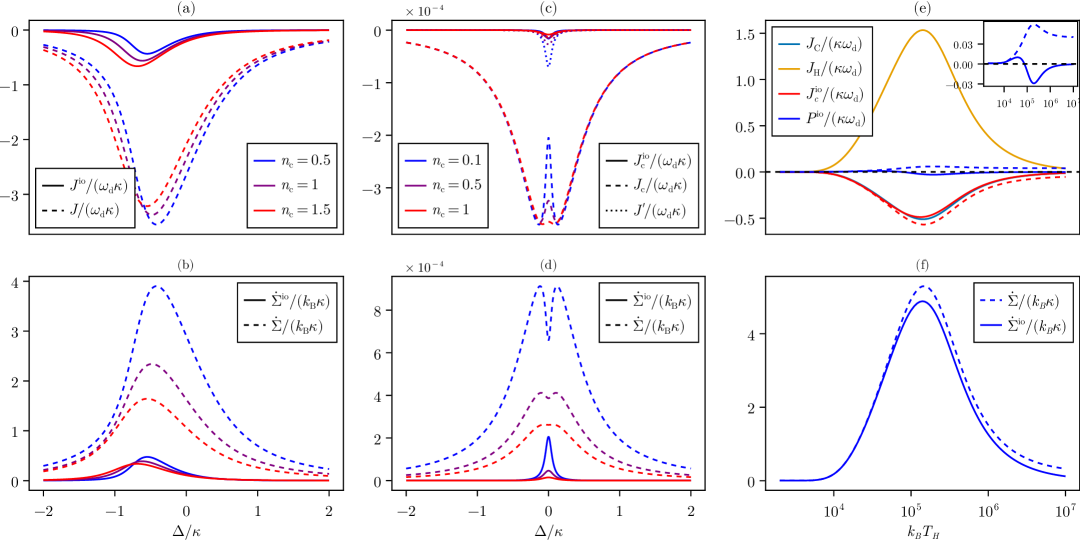
Figure 2: Conventional and new definitions of heat and work. For (a-d) $\Omega/\kappa=10^{4}$, $\gamma/\kappa=0.05$, $g/\kappa=0.1$, $f/\kappa=0.01$. (a) Heat current and (b) entropy production for the Kerr oscillator for different occupation numbers $n_{\rm c}$ as a function of detuning $\Delta=\Omega-\omega_{\rm d}$. Note that $P^{({\rm io})}=-J^{({\rm io})}$. Parameters: $\Omega/\kappa=10^{4}$, $K/\kappa=0.05$, $f/\kappa=1$. (c) Heat currents and (d) entropy production for the two-level system for different occupation numbers as a function of detuning. (e-f) Heat currents and power, and entropy production for the quantum three-level maser; $\Omega/\kappa=10^{4},~g/\kappa=0.7,~f/\kappa=0.1,~\omega_{2}/\kappa=\omega_{3}/(3\kappa)=\Omega/\kappa,~\gamma_{H}/\kappa=0.5,~\gamma_{C}/\kappa=100,~n_{c}=4.54,~n_{C}=0.007$. (e) We observe that there is region, $k_{B}T_{H}\approx 10^{5}$ in which the system is a heat engine, $P^{\text{io}}<0$, while $P>0$ (see also inset). The dashed black line indicates the zero. (f) Entropy production is peaked at the heat engine regime.

Kerr oscillator – As a second, nonlinear example we consider a Kerr Oscillator described by

$$\hat{H}^{\prime}=K\hat{a}^{\dagger}\hat{a}^{\dagger}\hat{a}\hat{a}\operatorname{~.}$$ (25)

We do not consider additional losses $\mathcal{L}^{\prime}=0$ and we consider the thermodynamic Hamiltonian $\hat{H}_{\rm TD}=\omega_{\rm d}\hat{a}^{\dagger}\hat{a}$ which assigns each photon within the cavity the energy $\omega_{\rm d}$. We note that this requires $K\ll\omega_{\rm d}$ such that a constant thermal occupation $n_{\rm c}$ is justified even though the cavity frequency effectively depends on the number of photons within the cavity. We compare the conventional definitions of heat and work with our new definitions, see Fig. 2. As the temperature is increased, the conventional definition predicts a decrease in entropy production, because less photons can enter the cavity from the drive due to the photon-number dependence of the resonance frequency. In contrast, our new definition is much less sensitive to an increase in $n_{\rm c}$, since the entropy production only arises from a reduced coherence due to nonlinear effects. This illustrates how the two definitions provide different insight into irreversibility, depending on the accessibility of the output light.

Two-level system – As a next example, we consider a two-level system embedded in the cavity described by

$$\hat{H}^{\prime} =\frac{\Omega}{2}\hat{\sigma}_{\rm z}+g(\hat{a}^{\dagger}\hat{\sigma}_{-}+\hat{a}\hat{\sigma}_{+})\operatorname{~,}$$ (26)

$$\hat{H}_{\rm TD} =\omega_{\rm d}\left(\hat{a}^{\dagger}\hat{a}+\hat{\sigma}_{+}\hat{\sigma}_{-}\right)\operatorname{~,}$$ (27)

$$\mathcal{L}^{\prime} =\gamma n_{\rm q}\mathcal{D}[\hat{\sigma}_{+}]+\gamma(n_{\rm q}+1)\mathcal{D}[\hat{\sigma}_{-}]\operatorname{~,}$$ (28)

where $g$ is the coupling between the cavity and the qubit, $\gamma$ and $n_{\rm q}=[e^{\omega_{d}/(k_{\rm B}T_{\rm q})}-1]^{-1}$ denote the coupling and the occupation of an additional thermal reservoir coupled to the qubit, and the system operators of the two-level system are given by $\hat{\sigma}_{\rm z}=\outerproduct{e}{e}-\outerproduct{g}{g}\operatorname{~,}~\hat{\sigma}_{-}=\outerproduct{g}{e}=\hat{\sigma}_{+}^{\dagger}$. The thermodynamic Hamiltonian assigns each excitation the same energy $\omega_{\rm d}$.

We find that the additional heat current for the intra–cavity system can be expressed as follows,

$$J^{\prime}=\omega_{\rm d}\gamma\frac{n_{\rm q}}{n_{\rm F}}(n_{\rm F}-\langle\hat{\sigma}_{+}\hat{\sigma}_{-}\rangle)\operatorname{~,}$$ (29)

where $n_{\rm F}=[e^{\omega_{d}/(k_{\rm B}T_{\rm q})}+1]^{-1}$ denotes the Fermi-Dirac occupation. Here we focus on a single-temperature environment $n_{\rm c}=n_{\rm q}$.

For a weak drive on resonance ($\Delta=0$), the light emitted by the two-level system destructively interferes with the drive, preventing the cavity from being filled [32]. As a consequence, the conventional entropy production is reduced. In contrast, our new definition shows a peak in the entropy production at $\Delta=0$ because part of the light is dissipated through the two-level system. Increasing temperature suppresses coherence in the two-level system. As a consequence, the features resulting from destructive interference are suppressed and we find a finite $J^{\rm io}$ as the coherence of the light is reduced.

Three-level maser— The three-level maser is a canonic example of a quantum heat engine [33, 20, 16, 34, 13, 35, 36]. It can be described by

$$H^{\prime} =\omega_{3}\outerproduct{3}{3}+\omega_{2}\outerproduct{2}{2}+g(\hat{a}\outerproduct{2}{1}+\hat{a}^{\dagger}\outerproduct{1}{2}),$$ (30)

$$H_{\text{TD}} =\omega_{\rm d}(\hat{a}^{\dagger}\hat{a}+\outerproduct{2}{2})+\omega_{3}\outerproduct{3}{3},$$ (31)

with $\omega_{3}>\omega_{2}$. The thermodynamic Hamiltonian extends the two-level case by adding the state $\ket{3}$. Dissipation is described by $\mathcal{L}^{\prime}=\mathcal{L}_{\text{H}}+\mathcal{L}_{\text{C}}$, with

$$\mathcal{L}_{\text{H}} =\gamma_{H}n_{\text{H}}\mathcal{D}[\outerproduct{3}{1}]+\gamma_{H}(n_{\rm H}+1)\mathcal{D}[\outerproduct{1}{3}],$$ (32)

$$\mathcal{L}_{\text{C}} =\gamma_{C}n_{\text{C}}\mathcal{D}[\outerproduct{3}{2}]+\gamma_{C}(n_{\rm C}+1)\mathcal{D}[\outerproduct{2}{3}],$$ (33)

where $n_{\rm H}=[e^{\omega_{3}/(k_{\rm B}T_{\rm H})}-1]^{-1}$, $n_{\rm C}=[e^{(\omega_{3}-\omega_{\rm d})/(k_{\rm B}T_{\rm C})}-1]^{-1}$, and $T_{\rm H}>T_{\rm C}$ creates a population inversion between the states $\ket{1}$ and $\ket{2}$. Due to the quantum mechanical treatment of the cavity field, the conventional definitions of heat and work predicts $P>0$ and suggests that the system ceases to operate as a heat engine, see Fig. 2 (e) [16, 13]. The reason for this is the energetic cost of maintaining coherence in the cavity. Our new framework resolves this flaw, as there is no energetic cost to maintain coherence when the output light can be further used, identifying regions in which $P_{\text{io}}<0$. In these regions, a heat current between hot and cold baths increases the coherence in the output light.

Conclusions and outlook – We have shown how treating the output light of a coherently driven system as accessible leads to a consistent thermodynamic framework. This framework features a second law that is strictly tighter than the conventional approach. Without an additional entropy source, our second law implies that the noise in the output light is always larger than the noise in the input light. Our framework is thus particularly promising for investigating the noise properties of cascaded systems and opens up novel ways of investigating the thermodynamics of optical devices such as circulators and amplifiers. An avenue of particular interest is provided by the thermodynamics of non-reciprocal devices [37].

Our formalism only treats the coherent part of the output light as accessible. This requires the presence of a phase reference. Quantifying work in the output light in the absence of a perfect phase reference remains an open problem. Another promising avenue is to investigate fluctuations of heat and work in the new framework, which would allow for investigating fluctuation theorems [1] and thermodynamic uncertainty relations [38].

In this Supplemental Material, we provide additional information and calculations to the statements made in the Letter. In Sec. I, we show how the power is obtained from the thermodynamic Hamiltonian. Section II illustrates the assumptions that result in the decomposition of heat given in Eq. (11). In Sec. III, we provide the power and the heat current of the cavity using input-output operators. Section IV provides proofs for the second law of thermodynamics in both the conventional and the new framework.

I I. Power from the Thermodynamic Hamiltonian

I.1 Conventional framework

We show that the commutator of the thermodynamic Hamiltonian $\hat{H}_{\rm TD}=\omega_{\rm d}\hat{a}^{\dagger}\hat{a}+H_{\rm TD}^{\prime}$ with the full system Hamiltonian $\hat{H}(t)$ is approximately given by the time derivative of the full system Hamiltonian $\partial_{t}\hat{H}(t)$

$$[\hat{H}_{\rm TD},\hat{H}(t)]=[\omega_{\rm d}\hat{a}^{\dagger}\hat{a},\hat{H}_{\rm d}(t)]+[\hat{H}_{\rm TD},\hat{H}^{\prime}(t)]+[\hat{H}_{\rm TD}^{\prime},\Omega\hat{a}^{\dagger}\hat{a}]+[\hat{H}_{\rm TD}^{\prime},\hat{H}_{\rm d}(t)].$$ (S1)

We now use the assumptions that the thermodynamic Hamiltonian of the intra–cavity system commutes with the cavity mode, i.e., $[\hat{a},\hat{H}_{\rm TD}^{\prime}]=0$. As a consequence

$$[\hat{H}_{\rm TD}^{\prime},\hat{H}_{\rm d}(t)]=[\hat{H}_{\rm TD}^{\prime},\Omega\hat{a}^{\dagger}\hat{a}]=0\operatorname{~,}$$ (S2)

we further assume that

$$[\hat{H}_{\rm TD},\hat{H}^{\prime}(t)]\simeq\partial_{t}\hat{H}^{\prime}(t)\operatorname{~.}$$ (S3)

For the final term of Eq. (S1) we find

$$[\omega_{\rm d}\hat{a}^{\dagger}\hat{a},\hat{H}_{\rm d}]=-i\omega_{\rm d}\sqrt{\kappa}\left(\langle\hat{b}_{\rm in}^{\dagger}(t)\rangle\hat{a}+\langle\hat{b}_{\rm in}(t)\rangle\hat{a}^{\dagger}\right)\operatorname{~.}$$ (S4)

For $\langle\hat{b}_{\rm in}(t)\rangle=f(t)e^{-i\omega_{\rm d}t}$, we find

$$-i[\omega_{\rm d}\hat{a}^{\dagger}\hat{a},\hat{H}_{\rm d}(t)]\simeq\partial_{t}\hat{H}_{\rm d}(t)\operatorname{~,}$$ (S5)

as long as $\omega_{\rm d}|f(t)|\gg|\partial_{t}f(t)|$ such that we can neglect the time derivative of $f(t)$ in Eq. (S5).

Together, the above relations provide

$$-i[\hat{H}_{\rm TD},\hat{H}(t)]\simeq\partial_{t}\hat{H}(t)\operatorname{~.}$$ (S6)

I.2 New framework

For the new framework, the calculation goes analogously. However, the drive Hamiltonian needs to be replaced with [c.f. Eq. (19)]

$$\hat{H}_{\rm s}=i\frac{\sqrt{\kappa}}{2}\left(\left[\langle\operatorname{\hat{\textit{b}}_{\text{in}}^{\dagger}}(t)\rangle+\langle\operatorname{\hat{\textit{b}}_{\text{out}}^{\dagger}}(t)\rangle\right]\hat{a}-\left[\langle\operatorname{\hat{\textit{b}}_{\text{in}}}(t)\rangle+\langle\operatorname{\hat{\textit{b}}_{\text{out}}}(t)\rangle\right]\hat{a}^{\dagger}\right)\operatorname{~.}$$ (S7)

As long as $\langle\hat{a}\rangle(t)=\alpha(t)e^{-i\omega_{\rm d}t}$, where $\alpha(t)$ is a slowly varying function such that $\omega_{\rm d}|\alpha(t)|\gg\partial_{t}\alpha(t)$, we find again

$$-i[\omega_{\rm d}\hat{a}^{\dagger}\hat{a},\hat{H}_{\rm s}]\simeq\partial_{t}\hat{H}_{\rm s}(t)\operatorname{~,}$$ (S8)

such that power can still be expressed through the time-derivative of the Hamiltonian.

II II. Decomposition of Heat

The heat current given in Eq. (10) can be written as as

$$J=\Tr{\hat{H}_{\rm TD}\mathcal{L}\rho(t)}=\Tr{\omega_{\rm d}\hat{a}^{\dagger}\hat{a}\mathcal{L}_{\rm c}\rho(t)}+\Tr{\omega_{\rm d}\hat{a}^{\dagger}\hat{a}\mathcal{L}^{\prime}\rho(t)}+\Tr{\hat{H}_{\rm TD}^{\prime}\mathcal{L}_{\rm c}\rho(t)}+\Tr{\hat{H}_{\rm TD}^{\prime}\mathcal{L}^{\prime}\rho(t)}\operatorname{~.}$$ (S9)

From $[\hat{a},\hat{H}_{\rm TD}^{\prime}]=0$ one may show that

$$\Tr{\hat{H}_{\rm TD}^{\prime}\mathcal{L}_{\rm c}\rho(t)}=0\operatorname{~.}$$ (S10)

In addition, we write

$$\mathcal{L}^{\prime}\hat{\rho}=\sum_{k}\mathcal{D}[\hat{L}_{k}]\hat{\rho},$$ (S11)

and we assume that $[\hat{L}_{k},\hat{a}^{(\dagger)}]=0$. It follows that

$$\Tr{\omega_{\rm d}\hat{a}^{\dagger}\hat{a}\mathcal{L}^{\prime}\rho(t)}=0\operatorname{~.}$$ (S12)

We thus find the decomposition of heat provided in the main text

$$J=\Tr{\omega_{\rm d}\hat{a}^{\dagger}\hat{a}\mathcal{L}_{\rm c}\rho(t)}+\Tr{\hat{H}_{\rm TD}^{\prime}\mathcal{L}^{\prime}\rho(t)}=J_{\rm c}+J^{\prime}\operatorname{~.}$$ (S13)

We note that this decomposition analogously holds for the new framework, where we need to replace $\mathcal{L}_{\rm c}\rightarrow\mathcal{L}_{\rm s}$.

III III. Energy exchanged with the input and output fields

We consider the sum of $P$ and $J_{\rm c}$,

$$P+J_{\rm c}=-\sqrt{\kappa}\omega_{\rm d}\bigg{(}\langle\hat{b}_{\text{in}}^{\dagger}(t)\rangle\langle\hat{a}\rangle+\langle\hat{b}_{\text{in}}(t)\rangle\langle\hat{a}^{\dagger}\rangle\bigg{)}+\omega_{\rm d}\kappa(n_{\rm B}-\langle\hat{a}^{\dagger}\hat{a}\rangle)\operatorname{~,}$$ (S14)

We may eliminate the cavity operator using $\sqrt{\kappa}\hat{a}=\operatorname{\hat{\textit{b}}_{\text{out}}}-\operatorname{\hat{\textit{b}}_{\text{in}}}$ (for ease of notation we suppress the time arguments) to find,

$$P+J_{\rm c} =\omega_{\rm d}\kappa n_{\rm B}-\omega_{\rm d}\bigg{(}\langle\hat{b}_{\text{in}}^{\dagger}\rangle\langle\operatorname{\hat{\textit{b}}_{\text{out}}}\rangle-\langle\hat{b}_{\text{in}}^{\dagger}\rangle\langle\operatorname{\hat{\textit{b}}_{\text{in}}}\rangle+\langle\hat{b}_{\text{in}}\rangle\langle\operatorname{\hat{\textit{b}}_{\text{out}}^{\dagger}}\rangle-\langle\hat{b}_{\text{in}}(t)\rangle\langle\operatorname{\hat{\textit{b}}_{\text{in}}^{\dagger}}\rangle\bigg{)}$$ (S15)

$$~~-\omega_{\rm d}\bigg{(}\langle\operatorname{\hat{\textit{b}}_{\text{out}}^{\dagger}}\operatorname{\hat{\textit{b}}_{\text{out}}}\rangle-\langle\operatorname{\hat{\textit{b}}_{\text{out}}^{\dagger}}\operatorname{\hat{\textit{b}}_{\text{in}}}\rangle-\langle\operatorname{\hat{\textit{b}}_{\text{in}}^{\dagger}}\operatorname{\hat{\textit{b}}_{\text{out}}}\rangle+\langle\operatorname{\hat{\textit{b}}_{\text{in}}^{\dagger}}\operatorname{\hat{\textit{b}}_{\text{in}}}\rangle\bigg{)}$$

$$=\omega_{\rm d}\bigg{(}\kappa n_{\rm B}-\langle\operatorname{\hat{\textit{b}}_{\text{out}}^{\dagger}}\operatorname{\hat{\textit{b}}_{\text{out}}}\rangle+\langle\operatorname{\hat{\textit{b}}_{\text{in}}^{\dagger}}\operatorname{\hat{\textit{b}}_{\text{in}}}\rangle+\langle\!\langle\operatorname{\hat{\textit{b}}_{\text{out}}^{\dagger}}\operatorname{\hat{\textit{b}}_{\text{in}}}\rangle\!\rangle+\langle\!\langle\operatorname{\hat{\textit{b}}_{\text{out}}}\operatorname{\hat{\textit{b}}_{\text{in}}^{\dagger}}\rangle\!\rangle-2\langle\!\langle\hat{b}_{\text{in}}\operatorname{\hat{\textit{b}}_{\text{in}}^{\dagger}}\rangle\!\rangle\bigg{)}$$

Using the relation $\langle\!\langle\operatorname{\hat{\textit{b}}_{\text{in}}^{\dagger}}\hat{a}\rangle\!\rangle=\langle\!\langle\hat{a}^{\dagger}\operatorname{\hat{\textit{b}}_{\text{in}}}\rangle\!\rangle=-\sqrt{\kappa}\frac{n_{B}}{2}$ [17], we find

$$\langle\!\langle\operatorname{\hat{\textit{b}}_{\text{out}}^{\dagger}}\operatorname{\hat{\textit{b}}_{\text{in}}}\rangle\!\rangle=\langle\!\langle\operatorname{\hat{\textit{b}}_{\text{in}}^{\dagger}}\operatorname{\hat{\textit{b}}_{\text{out}}}\rangle\!\rangle=\langle\!\langle\operatorname{\hat{\textit{b}}_{\text{in}}^{\dagger}}\operatorname{\hat{\textit{b}}_{\text{in}}}\rangle\!\rangle-\frac{{\kappa}}{2}n_{B}\operatorname{~,}$$ (S16)

which results in

$$P+J_{\rm c}=\omega_{\rm d}\left(\langle\operatorname{\hat{\textit{b}}_{\text{out}}^{\dagger}}(t)\operatorname{\hat{\textit{b}}_{\text{out}}}(t)\rangle-\langle\operatorname{\hat{\textit{b}}_{\text{in}}^{\dagger}}(t)\operatorname{\hat{\textit{b}}_{\text{in}}}(t)\rangle\right)=P^{\rm io}+J^{\rm io}.$$ (S17)

Similarly, we may use $\sqrt{\kappa}\hat{a}=\operatorname{\hat{\textit{b}}_{\text{out}}}-\operatorname{\hat{\textit{b}}_{\text{in}}}$ and Eq. (S16) to show

$$J_{\rm c}^{\rm io}=-\omega_{\rm d}\left(\langle\!\langle\operatorname{\hat{\textit{b}}_{\text{out}}^{\dagger}}(t)\operatorname{\hat{\textit{b}}_{\text{out}}}(t)\rangle\!\rangle-\langle\!\langle\operatorname{\hat{\textit{b}}_{\text{in}}^{\dagger}}(t)\operatorname{\hat{\textit{b}}_{\text{in}}}(t)\rangle\!\rangle\right)=\omega_{\rm d}\kappa(n_{\rm B}-\langle\!\langle\hat{a}^{\dagger}\hat{a}\rangle\!\rangle).$$ (S18)

IV IV. Proof of the second law of thermodynamics

To prove the second law of thermodynamics, we use Spohn’s inequality [27],

$$-\Tr{\mathcal{L}\rho(t)\quantity[\ln\rho(t)-\ln\hat{\sigma}]}\geq 0\operatorname{~,}$$ (S19)

where $\mathcal{L}$ is the generator of a positive semi group and $\hat{\sigma}$ is its steady state, i.e., $\mathcal{L}\hat{\sigma}=0$.

IV.1 Conventional framework

We introduce thesteady states of the dissipators in the master equation in Eq. (4)

$$\mathcal{L}_{\rm c}\hat{\sigma}_{\rm c}=\mathcal{L}^{\prime}\hat{\sigma}^{\prime}=0,$$ (S20)

with

$$\hat{\sigma}_{\rm c}=\frac{e^{-\omega_{\rm d}\hat{a}^{\dagger}\hat{a}/(k_{\rm B}T_{\rm c})}}{{\rm Tr}\left\{e^{-\omega_{\rm d}\hat{a}^{\dagger}\hat{a}/(k_{\rm B}T_{\rm c})}\right\}},\hskip 42.67912pt\hat{\sigma}^{\prime}=\frac{e^{-\hat{H}_{\rm TD}^{\prime}/(k_{\rm B}T^{\prime})}}{{\rm Tr}\left\{e^{-\hat{H}_{\rm TD}^{\prime}/(k_{\rm B}T^{\prime})}\right\}}.$$ (S21)

While $\hat{\sigma}_{\rm c}$ is determined by our choice of $\mathcal{L}_{\rm c}$, c.f. Eq. (5), the stationary state $\hat{\sigma}^{\prime}$ is assumed to be consistent with the thermodynamic Hamiltonian.

The heat currents $J_{\rm c}$ and $J^{\prime}$ may consequently be written in terms of the dissipators and their stationary states

$$J_{\rm c}=-k_{\rm B}T_{\rm c}\Tr{\mathcal{L}_{\rm c}\rho(t)\ln\hat{\sigma}_{\rm c}}\operatorname{~,}\hskip 42.67912ptJ^{\prime}=-k_{\rm B}T^{\prime}\Tr{\mathcal{L}^{\prime}\rho(t)\ln\hat{\sigma}^{\prime}}\operatorname{~.}$$ (S22)

Substituting these heat currents into Eq. (8) results in

$$\dot{\Sigma}/k_{\rm B}=\partial_{t}S_{\text{vN}}(\rho(t))+\Tr{\mathcal{L}_{\rm c}\rho(t)\ln\hat{\sigma}_{\rm c}}+\Tr{\mathcal{L}^{\prime}\rho(t)\ln\hat{\sigma}^{\prime}}\operatorname{~,}$$ (S23)

which in turn can be written as

$$\dot{\Sigma}/k_{\rm B} =-\Tr{\mathcal{L}\rho(t)\ln\rho(t)}+\Tr{\mathcal{L}_{\rm c}\rho(t)\ln\hat{\sigma}_{\rm c}}+\Tr{\mathcal{L}^{\prime}\rho(t)\ln\hat{\sigma}^{\prime}}$$

$$=-\Tr{\mathcal{L}_{\rm c}\rho(t)\quantity[\ln\hat{\rho}(t)-\ln\hat{\sigma}_{\rm c}]}-\Tr{\mathcal{L}^{\prime}\rho(t)\quantity[\ln\hat{\rho}(t)-\ln\hat{\sigma}^{\prime}\ ]}\geq 0\operatorname{~.}$$ (S24)

The result on the right hand side is a sum of two Spohn inequalities, see Eq. (S19). Therefore we have proven that the entropy production rate is indeed non-negative and the second law is verified for the conventional definitions of power and heat.

IV.2 New framework

To derive the second law for the new framework we show that we can still write the new definition of the heat current as we do in equation (S22). To this end, we introduce the steady state of the shifted dissipator

$$\mathcal{L}_{\rm s}\hat{\sigma}_{\rm s}=0,\hskip 42.67912pt\hat{\sigma}_{\rm s}=\frac{e^{-\omega_{\rm d}\left(\hat{a}^{\dagger}-\langle\hat{a}^{\dagger}\rangle)(\hat{a}-\langle\hat{a}\rangle\right)/\left(k_{\rm B}T_{\rm c}\right)}}{{\rm Tr}\left\{e^{-\omega_{\rm d}\left(\hat{a}^{\dagger}-\langle\hat{a}^{\dagger}\rangle)(\hat{a}-\langle\hat{a}\rangle\right)/\left(k_{\rm B}T_{\rm c}\right)}\right\}}\operatorname{~,}$$ (S25)

The new definition of the heat current is given by

$$J_{\rm c}^{\rm io}=\Tr{\omega_{\rm d}\hat{a}^{\dagger}\hat{a}\mathcal{L}_{\rm s}\rho(t)}$$ (S26)

We use the relations

$$\Tr{\hat{a}\mathcal{L}_{\rm s}\rho(t)}=\Tr{\hat{a}^{\dagger}\mathcal{L}_{\rm s}\rho(t)}=\Tr{\mathcal{L}_{\rm s}\rho(t)}=0\operatorname{~,}$$ (S27)

to show that the heat current can be written as

$$J_{\rm c}^{\rm io}=\Tr{\omega_{\rm d}(\hat{a}^{\dagger}-\langle\hat{a}^{\dagger}\rangle)(\hat{a}-\langle\hat{a}\rangle)\mathcal{L}_{\rm s}\rho(t)}=-k_{\rm B}T_{\rm c}\Tr{\mathcal{L}_{\rm s}\rho(t)\ln\hat{\sigma}_{\rm s}}\operatorname{~.}$$ (S28)

The second law then follows analogously to how it is derived above for the conventional framework by writing

$$\dot{\Sigma}^{\rm io}\equiv k_{\rm B}\partial_{t}S_{\rm vN}(\rho(t))-\frac{J_{\rm c}^{\rm io}}{T_{\rm c}}-\frac{J^{\prime}}{T^{\prime}}=-k_{\rm B}\Tr{\mathcal{L}_{\rm s}\rho(t)\quantity[\ln\hat{\rho}(t)-\ln\hat{\sigma}_{\rm s}]}-k_{\rm B}\Tr{\mathcal{L}^{\prime}\rho(t)\quantity[\ln\hat{\rho}(t)-\ln\hat{\sigma}^{\prime}\ ]}\geq 0\operatorname{~.}$$ (S29)

We finally note that

$$\dot{\Sigma}-\dot{\Sigma}^{\rm io}=\frac{J_{\rm c}^{\rm io}-J_{\rm c}}{T_{\rm c}}=\frac{\omega_{d}\kappa}{T_{\rm c}}|\langle\hat{a}\rangle|^{2}\geq 0,$$ (S30)

V V. Generalization of the framework

V.1 Master equation and thermodynamic Hamiltonian

In this section, we extend the framework introduced in the main text to additional dissipation channels and multiple temperatures. To this end, we consider the master equation

$$\partial_{t}\hat{\rho}(t)=-i\quantity[\hat{H}(t),\hat{\rho}(t)]+\mathcal{L}\hat{\rho}(t)(t)\operatorname{~,}$$ (S31)

with the dissipator

$$\mathcal{L}=\sum_{j}\mathcal{L}_{{\rm c},j}+\sum_{k}\mathcal{L}_{k}+\sum_{l}\mathcal{L}_{l}^{\prime}.$$ (S32)

Here

$$\mathcal{L}_{{\rm c},j}\hat{\rho} =\kappa_{j}n_{{\rm c},j}\mathcal{D}[\hat{a}^{\dagger}]\hat{\rho}+\kappa_{j}(n_{{\rm c},j}+1)\mathcal{D}[\hat{a}]\hat{\rho}\operatorname{~,}$$ (S33)

denote photon loss due to output channels that are accessible. The coherent field leaking out into these channels are therefore interpreted as work. In addition, we consider inaccessible channels where photons are exchanged with the environment described by the dissipators

$$\mathcal{L}_{k}\hat{\rho} =\gamma_{k}n_{k}\mathcal{D}[\hat{a}^{\dagger}]\hat{\rho}+\gamma_{k}(n_{k}+1)\mathcal{D}[\hat{a}]\hat{\rho}.$$ (S34)

The dissipators $\mathcal{L}^{\prime}_{l}$ denote dissipation of the system embedded into the cavity. Splitting this dissipator into multiple parts allows us to consider reservoirs at different temperatures.

The Hamiltonian in Eq. (S31) reads

$$\hat{H}(t)=\Omega\hat{a}^{\dagger}\hat{a}+\hat{H}^{\prime}(t)+i\sum_{j}\sqrt{\kappa_{j}}\left(\langle\hat{b}^{\dagger}_{{\rm in},j}(t)\rangle\hat{a}-\langle\hat{b}_{{\rm in},j}(t)\rangle\hat{a}^{\dagger}\right)+i\sum_{k}\sqrt{\gamma_{k}}\left(\langle\hat{c}^{\dagger}_{{\rm in},k}(t)\rangle\hat{a}-\langle\hat{c}_{{\rm in},k}(t)\rangle\hat{a}^{\dagger}\right),$$ (S35)

where $\hat{b}_{{\rm in},j}$ and $\hat{c}_{{\rm in},j}$ denote the input modes of the observed and unobserved channels respectively. Note that we also allow $\hat{H}^{\prime}(t)$ to be explicitly time-dependent. As in the main text, we leave $\hat{H}^{\prime}(t)$ and $\mathcal{L}_{l}^{\prime}$ unspecified but we assume that a thermodynamic description based on a single thermodynamic Hamiltonian exists. To this end, we make the following assumptions

$${\rm Tr}\left\{\hat{a}^{\dagger}\hat{a}\mathcal{L}^{\prime}_{l}\hat{\rho}\right\}={\rm Tr}\left\{\hat{a}^{(\dagger)}\mathcal{L}^{\prime}_{l}\hat{\rho}\right\}=0.$$ (S36)

We use the same thermodynamic Hamiltonian as in the main text

$$\hat{H}_{\rm TD}=\omega_{\rm d}\hat{a}^{\dagger}\hat{a}+\hat{H}_{\rm TD}^{\prime}\operatorname{~,}$$ (S37)

where we assume that

$$[\hat{H}_{\rm TD}^{\prime},\hat{a}]=0,\hskip 56.9055pt\mathcal{L}_{l}^{\prime}\hat{\sigma}^{\prime}_{l}=0,\hskip 14.22636pt\hat{\sigma}^{\prime}_{l}=\frac{e^{-\hat{H}_{\rm TD}^{\prime}/(k_{\rm B}T^{\prime}_{l})}}{{\rm Tr}\left\{e^{-\hat{H}_{\rm TD}^{\prime}/(k_{\rm B}T^{\prime}_{l})}\right\}}.$$ (S38)

In addition, one may show that

$$\mathcal{L}_{{\rm c},j}\hat{\sigma}_{{\rm c},j}=0,\hskip 14.22636pt\mathcal{L}_{k}\hat{\sigma}_{k}=0,\hskip 14.22636pt\hat{\sigma}_{{\rm c},j}=\frac{e^{-\omega_{\rm d}\hat{a}^{\dagger}\hat{a}/(k_{\rm B}T_{{\rm c},j})}}{{\rm Tr}\left\{e^{-\omega_{\rm d}\hat{a}^{\dagger}\hat{a}/(k_{\rm B}T_{{\rm c},j})}\right\}},\hskip 14.22636pt\hat{\sigma}_{k}=\frac{e^{-\omega_{\rm d}\hat{a}^{\dagger}\hat{a}/(k_{\rm B}T_{k})}}{{\rm Tr}\left\{e^{-\omega_{\rm d}\hat{a}^{\dagger}\hat{a}/(k_{\rm B}T_{k})}\right\}},$$ (S39)

where

$$n_{{\rm c},j}=\frac{1}{e^{\omega_{d}/(k_{\rm B}T_{{\rm c},j})}-1},\hskip 28.45274ptn_{k}=\frac{1}{e^{\omega_{d}/(k_{\rm B}T_{k})}-1}.$$ (S40)

We further assume that

$$-i[\hat{H}_{\rm TD},\hat{H}(t)]\simeq\partial_{t}\hat{H}(t).$$ (S41)

This is the case as long as $-i[\hat{H}_{\rm TD},\hat{H}^{\prime}(t)]\simeq\partial_{t}\hat{H}^{\prime}(t)$ and all input drives only contain frequencies close to $\omega_{\rm d}$. If the input drives contain frequencies far from $\omega_{\rm d}$, we may always drop them as they will not be able to enter the cavity in the first place. Indeed, we may choose $\omega_{\rm d}=\Omega$, in particular if there is no unique drive frequency.

V.2 Conventional framework

Like in the main text, the first law reads

$$\partial_{t}\langle\hat{H}_{\rm TD}\rangle=P+J,\hskip 42.67912ptP=-i\langle[\hat{H}_{\rm TD},\hat{H}(t)]\rangle,\hskip 14.22636ptJ={\rm Tr}\left\{\hat{H}_{\rm TD}\mathcal{L}\hat{\rho}(t)\right\}.$$ (S42)

With the assumptions above, we may divide the power into different contributions

$$P=\sum_{j}P_{{\rm c},j}+\sum_{k}P_{k}+P^{\prime},$$ (S43)

with

$$P_{{\rm c},j}=-\sqrt{\kappa_{j}}\omega_{\rm d}\bigg{(}\langle\hat{b}_{\text{in},j}^{\dagger}(t)\rangle\langle\hat{a}\rangle+\langle\hat{b}_{\text{in},j}(t)\rangle\langle\hat{a}^{\dagger}\rangle\bigg{)},\hskip 14.22636ptP_{k}=-\sqrt{\gamma_{k}}\omega_{\rm d}\bigg{(}\langle\hat{c}_{k}^{\dagger}(t)\rangle\langle\hat{a}\rangle+\langle\hat{c}_{k}(t)\rangle\langle\hat{a}^{\dagger}\rangle\bigg{)},$$ (S44)

and

$$P^{\prime}=-i\langle[\hat{H}_{\rm TD}^{\prime},\hat{H}^{\prime}(t)]\rangle.$$ (S45)

Similarly, heat can be divided as

$$J=\sum_{j}J_{{\rm c},j}+\sum_{k}J_{k}+\sum_{l}J^{\prime}_{l},$$ (S46)

with

$$J_{{\rm c},j}=\omega_{\rm d}\kappa_{j}(n_{{\rm c},j}-\langle\hat{a}^{\dagger}\hat{a}\rangle),\hskip 42.67912ptJ_{k}=\omega_{\rm d}\gamma_{k}(n_{k}-\langle\hat{a}^{\dagger}\hat{a}\rangle),\hskip 42.67912ptJ^{\prime}_{l}={\rm Tr}\left\{\hat{H}^{\prime}_{\rm TD}\mathcal{L}^{\prime}_{l}\hat{\rho}(t)\right\}.$$ (S47)

The second law of thermodynamics may be written as

$$\dot{\Sigma}\equiv k_{\rm B}\partial_{t}S_{\rm vN}(\hat{\rho})-\sum_{j}\frac{J_{{\rm c},j}}{T_{{\rm c},j}}-\sum_{k}\frac{J_{k}}{T_{k}}-\sum_{l}\frac{J^{\prime}_{l}}{T^{\prime}_{l}}\geq 0.$$ (S48)

It can be proven by casting the entropy production into

$$\dot{\Sigma}/{k_{\rm B}}=-\sum_{j}\Tr{\mathcal{L}_{{\rm c},j}\rho(t)\quantity[\ln\hat{\rho}(t)-\ln\hat{\sigma}_{{\rm c},j}]}-\sum_{k}\Tr{\mathcal{L}_{k}\rho(t)\quantity[\ln\hat{\rho}(t)-\ln\hat{\sigma}_{k}]}-\sum_{l}\Tr{\mathcal{L}^{\prime}_{l}\rho(t)\quantity[\ln\hat{\rho}(t)-\ln\hat{\sigma}^{\prime}_{l}\ ]},$$ (S49)

and using Spohn’s inequality.

V.3 New framework

In the new framework, the first law reads

$$\partial_{t}\langle\hat{H}_{\rm TD}\rangle=\sum_{j}\left(P_{{\rm c},j}^{\rm io}+J_{{\rm c},j}^{\rm io}\right)+\sum_{k}\left(P_{k}+J_{k}\right)+P^{\prime}+\sum_{l}J_{l}^{\prime},$$ (S50)

where

$$P_{{\rm c},j}^{\rm io}=-\omega_{\rm d}\left(|\langle\hat{b}_{{\rm out},j}(t)\rangle|^{2}-|\langle\hat{b}_{{\rm in},j}(t)\rangle|^{2}\right),\hskip 42.67912ptJ_{{\rm c},j}^{\rm io}=-\omega_{\rm d}\left(\langle\!\langle\hat{b}_{{\rm out},j}^{\dagger}(t)\hat{b}_{{\rm out},j}(t)\rangle\!\rangle-\langle\!\langle\hat{b}_{{\rm in},j}^{\dagger}(t)\hat{b}_{{\rm in},j}(t)\rangle\!\rangle\right),$$ (S51)

and the other terms remain the same as in the conventional framework. Note that we only altered the terms that correspond to output channels that we assume are accessible. In a straightforward generalization of the derivation given in Sec. III above, we find

$$P_{{\rm c},j}^{\rm io}+J_{{\rm c},j}^{\rm io}=P_{{\rm c},j}+J_{{\rm c},j},$$ (S52)

and

$$J_{{\rm c},j}^{\rm io}=\omega_{\rm d}\kappa_{j}(n_{{\rm c},j}-\langle\!\langle\hat{a}^{\dagger}\hat{a}\rangle\!\rangle).$$ (S53)

As in the main text, we obtain the laws of thermodyanmics from re-writing the master equation as

$$\partial_{t}\hat{\rho}(t)=-i\left[\hat{H}_{\rm s}(t),\hat{\rho}(t)\right]+\left[\sum_{j}\mathcal{L}_{{\rm s},j}+\sum_{k}\mathcal{L}_{k}+\sum_{l}\mathcal{L}_{l}^{\prime}\right]\hat{\rho}(t),$$ (S54)

with

$$\hat{H}_{\rm s}(t)=\hat{H}+\frac{i}{2}\sum_{j}\kappa_{j}\left(\langle\hat{a}^{\dagger}\rangle\hat{a}-\langle\hat{a}\rangle\hat{a}^{\dagger}\right),$$ (S55)

and

$$\mathcal{L}_{{\rm s},j}=\kappa_{j}n_{{\rm c},j}\mathcal{D}[\hat{a}^{\dagger}-\langle\hat{a}^{\dagger}\rangle]+\kappa_{j}(n_{{\rm c},j}+1)\mathcal{D}[\hat{a}-\langle\hat{a}\rangle].$$ (S56)

The steady state of this dissipator reads

$$\mathcal{L}_{{\rm s},j}\sigma_{\rm s}=0,\hskip 42.67912pt\sigma_{{\rm s},j}=\frac{e^{-\omega_{\rm d}\left(\hat{a}^{\dagger}-\langle\hat{a}^{\dagger}\rangle)(\hat{a}-\langle\hat{a}\rangle\right)/\left(k_{\rm B}T_{{\rm c},j}\right)}}{{\rm Tr}\left\{e^{-\omega_{\rm d}\left(\hat{a}^{\dagger}-\langle\hat{a}^{\dagger}\rangle)(\hat{a}-\langle\hat{a}\rangle\right)/\left(k_{\rm B}T_{{\rm c},j}\right)}\right\}}.$$ (S57)

The power and the contributions to the heat current may then be obtained through

$$-i\langle[\hat{H}_{\rm TD},\hat{H}_{\rm s}(t)]\rangle=\sum_{j}P_{{\rm c},j}^{\rm io}+\sum_{k}P_{k},\hskip 42.67912ptJ_{{\rm c},j}^{\rm io}={\rm Tr}\left\{\hat{H}_{\rm TD}\mathcal{L}_{{\rm s},j}\hat{\rho}(t)\right\}.$$ (S58)

The entropy production reads

$$\dot{\Sigma}^{\rm io}\equiv k_{\rm B}\partial_{t}S_{\rm vN}(\hat{\rho})-\sum_{j}\frac{J_{{\rm c},j}^{\rm io}}{T_{{\rm c},j}}-\sum_{k}\frac{J_{k}}{T_{k}}-\sum_{l}\frac{J^{\prime}_{l}}{T^{\prime}_{l}}\geq 0.$$ (S59)

And the second law is again proven using Spohn’s inequality by casting the entropy production into

$$\dot{\Sigma}/{k_{\rm B}}=-\sum_{j}\Tr{\mathcal{L}_{{\rm s},j}\rho(t)\quantity[\ln\hat{\rho}(t)-\ln\hat{\sigma}_{{\rm c},j}]}-\sum_{k}\Tr{\mathcal{L}_{k}\rho(t)\quantity[\ln\hat{\rho}(t)-\ln\hat{\sigma}_{k}]}-\sum_{l}\Tr{\mathcal{L}^{\prime}_{l}\rho(t)\quantity[\ln\hat{\rho}(t)-\ln\hat{\sigma}^{\prime}_{l}\ ]}.$$ (S60)

To this end, we used

$$\Tr{\omega_{\rm d}\hat{a}^{\dagger}\hat{a}\mathcal{L}_{{\rm s},j}\rho(t)}=\Tr{\omega_{\rm d}(\hat{a}^{\dagger}-\langle\hat{a}^{\dagger}\rangle)(\hat{a}-\langle\hat{a}\rangle)\mathcal{L}_{{\rm s},j}\rho(t)}.$$ (S61)

We further find

$$\dot{\Sigma}-\dot{\Sigma}^{\rm io}=\sum_{j}\frac{J_{{\rm c},j}^{\rm io}-J_{{\rm c},j}}{T_{{\rm c},j}}=\omega_{d}\sum_{j}\frac{\kappa_{j}}{T_{{\rm c},j}}|\langle\hat{a}\rangle|^{2}\geq 0,$$ (S62)

References

• Seifert [2012] U. Seifert, Stochastic thermodynamics, fluctuation theorems and molecular machines, Rep. Prog. Phys. 75, 126001 (2012).
• Van den Broeck and Esposito [2015] C. Van den Broeck and M. Esposito, Ensemble and trajectory thermodynamics: A brief introduction, Physica A 418, 6 (2015).
• Brandão et al. [2015] F. Brandão, M. Horodecki, N. Ng, J. Oppenheim, and S. Wehner, The second laws of quantum thermodynamics, Proc. Natl. Acad. Sci. U.S.A 112, 3275 (2015).
• Vinjanampathy and Anders [2016] S. Vinjanampathy and J. Anders, Quantum thermodynamics, Contemp. Phys. 57, 545–579 (2016).
• Binder et al. [2018] F. Binder, L. A. Correa, C. Gogolin, J. Anders, and G. Adesso, eds., Thermodynamics in the Quantum Regime (Springer, 2018).
• Deffner and Campbell [2019] S. Deffner and S. Campbell, Quantum Thermodynamics (Morgan & Claypool Publishers, 2019).
• Strasberg [2022] P. Strasberg, Quantum Stochastic Thermodynamics (Oxford University Press, 2022).
• Potts [2024] P. P. Potts, Quantum thermodynamics (2024), arXiv:2406.19206 [quant-ph] .
• Talkner et al. [2007] P. Talkner, E. Lutz, and P. Hänggi, Fluctuation theorems: Work is not an observable, Phys. Rev. E 75, 050102 (2007).
• Perarnau-Llobet et al. [2017] M. Perarnau-Llobet, E. Bäumer, K. V. Hovhannisyan, M. Huber, and A. Acin, No-go theorem for the characterization of work fluctuations in coherent quantum systems, Phys. Rev. Lett. 118, 070601 (2017).
• Kerremans et al. [2022] T. Kerremans, P. Samuelsson, and P. P. Potts, Probabilistically violating the first law of thermodynamics in a quantum heat engine, SciPost Phys. 12, 168 (2022).
• Elouard and Lombard Latune [2023] C. Elouard and C. Lombard Latune, Extending the laws of thermodynamics for arbitrary autonomous quantum systems, PRX Quantum 4, 020309 (2023).
• Niedenzu et al. [2019] W. Niedenzu, M. Huber, and E. Boukobza, Concepts of work in autonomous quantum heat engines, Quantum 3, 1 (2019).
• Gallego et al. [2016] R. Gallego, J. Eisert, and H. Wilming, Thermodynamic work from operational principles, New J. Phys. 18, 103017 (2016).
• Monsel et al. [2020] J. Monsel, M. Fellous-Asiani, B. Huard, and A. Auffèves, The energetic cost of work extraction, Phys. Rev. Lett. 124, 130601 (2020).
• Li et al. [2017] S. W. Li, M. B. Kim, G. S. Agarwal, and M. O. Scully, Quantum statistics of a single-atom Scovil-Schulz-DuBois heat engine, Phys. Rev. A 96, 1 (2017).
• Gardiner and Collett [1985] C. W. Gardiner and M. J. Collett, Input and output in damped quantum systems: Quantum stochastic differential equations and the master equation, Phys. Rev. A 31, 3761 (1985).
• [18] See the supplemental material below for a generalization of our framework, detailed derivations of the first and the second law, as well as proofs of statements used in the main text.
• Alicki [1979] R. Alicki, The quantum open system as a model of the heat engine, J. Phys. A: Math. Gen. 12, L103 (1979).
• Kosloff [1984] R. Kosloff, A quantum mechanical open system as a model of a heat engine, J. Chem. Phys. 80, 1625 (1984).
• Novotný [2002] T. Novotný, Investigation of apparent violation of the second law of thermodynamics in quantum transport studies, EPL 59, 648 (2002).
• Levy and Kosloff [2014] A. Levy and R. Kosloff, The local approach to quantum transport may violate the second law of thermodynamics, EPL 107, 20004 (2014).
• Trushechkin and Volovich [2016] A. S. Trushechkin and I. V. Volovich, Perturbative treatment of inter-site couplings in the local description of open quantum networks, EPL 113, 30005 (2016).
• Hofer et al. [2017] P. P. Hofer, M. Perarnau-Llobet, L. D. M. Miranda, G. Haack, R. Silva, J. B. Brask, and N. Brunner, Markovian master equations for quantum thermal machines: local versus global approach, New J. Phys. 19, 123037 (2017).
• González et al. [2017] J. O. González, L. A. Correa, G. Nocerino, J. P. Palao, D. Alonso, and G. Adesso, Testing the validity of the ‘local’ and ‘global’ GKLS master equations on an exactly solvable model, Open Syst. Inf. Dyn. 24, 1740010 (2017).
• Potts et al. [2021] P. Potts, A. A. S. Kalaee, and A. Wacker, A thermodynamically consistent Markovian master equation beyond the secular approximation, New J. Phys. 23, 123013 (2021).
• Spohn [1978] H. Spohn, Entropy production for quantum dynamical semigroups, J. Math. Phys. 19, 1227 (1978).
• Spohn and Lebowitz [1978] H. Spohn and J. L. Lebowitz, Irreversible thermodynamics for quantum systems weakly coupled to thermal reservoirs, in Advances in Chemical Physics, edited by S. Rice (John Wiley & Sons, Ltd, 1978).
• Prasad et al. [2024] S. P. Prasad, M. Maffei, P. A. Camati, C. Elouard, and A. Auffèves, Tracking light-matter correlations in the optical Bloch equations: Dynamics, energetics (2024), arXiv:2404.09648 [quant-ph] .
• Landi et al. [2024] G. T. Landi, M. J. Kewming, M. T. Mitchison, and P. P. Potts, Current fluctuations in open quantum systems: Bridging the gap between quantum continuous measurements and full counting statistics, PRX Quantum 5, 020201 (2024).
• Colla and Breuer [2022] A. Colla and H.-P. Breuer, Open-system approach to nonequilibrium quantum thermodynamics at arbitrary coupling, Phys. Rev. A 105, 052216 (2022).
• Auffèves-Garnier et al. [2007] A. Auffèves-Garnier, C. Simon, J.-M. Gérard, and J.-P. Poizat, Giant optical nonlinearity induced by a single two-level system interacting with a cavity in the purcell regime, Phys. Rev. A 75, 053823 (2007).
• Geusic et al. [1967] J. E. Geusic, E. O. Schulz-DuBios, and H. E. D. Scovil, Quantum equivalent of the carnot cycle, Phys. Rev. 156, 343 (1967).
• Dorfman et al. [2018] K. E. Dorfman, D. Xu, and J. Cao, Efficiency at maximum power of a laser quantum heat engine enhanced by noise-induced coherence, Phys. Rev. E 97, 042120 (2018).
• Mitchison [2019] M. T. Mitchison, Quantum thermal absorption machines: refrigerators, engines and clocks, Contemp. Phys. 60, 164 (2019).
• Kalaee et al. [2021] A. A. S. Kalaee, A. Wacker, and P. Potts, Violating the thermodynamic uncertainty relation in the three-level maser, Phys. Rev. E 104, L012103 (2021).
• Metelmann and Clerk [2015] A. Metelmann and A. A. Clerk, Nonreciprocal photon transmission and amplification via reservoir engineering, Phys. Rev. X 5, 021025 (2015).
• Horowitz and Gingrich [2020] J. M. Horowitz and T. R. Gingrich, Thermodynamic uncertainty relations constrain non-equilibrium fluctuations, Nat. Phys. 16, 15 (2020).
Supplemental Material: A Thermodynamic Framework for Coherently Driven Systems Max Schrauwen,1 Aaron Daniel,2 Marcelo Janovitch,2 Patrick P. Potts2 1 Department of Physics, RWTH Aachen University, 52056 Aachen, Germany
2 Department of Physics and Swiss Nanoscience Institute,
University of Basel, Klingelbergstrasse 82, 4056 Basel, Switzerland