OLinear: A Linear Model for Time Series Forecasting in Orthogonally Transformed Domain

Abstract

This paper presents OLinear, a linear-based multivariate time series forecasting model that operates in an orthogonally transformed domain. Recent forecasting models typically adopt the temporal forecast (TF) paradigm, which directly encode and decode time series in the time domain. However, the entangled step-wise dependencies in series data can hinder the performance of TF. To address this, some forecasters conduct encoding and decoding in the transformed domain using fixed, dataset-independent bases (e.g., sine and cosine signals in the Fourier transform). In contrast, we utilize OrthoTrans, a data-adaptive transformation based on an orthogonal matrix that diagonalizes the series’ temporal Pearson correlation matrix. This approach enables more effective encoding and decoding in the decorrelated feature domain and can serve as a plug-in module to enhance existing forecasters. To enhance the representation learning for multivariate time series, we introduce a customized linear layer, NormLin, which employs a normalized weight matrix to capture multivariate dependencies. Empirically, the NormLin module shows a surprising performance advantage over multi-head self-attention, while requiring nearly half the FLOPs. Extensive experiments on 24 benchmarks and 140 forecasting tasks demonstrate that OLinear consistently achieves state-of-the-art performance with high efficiency. Notably, as a plug-in replacement for self-attention, the NormLin module consistently enhances Transformer-based forecasters. The code and datasets are available at https://anonymous.4open.science/r/OLinear.

1 Introduction

Multivariate time series forecasting is critical in fields such as weather (Wu et al., 2023a), transportation (Ma et al., 2021), energy (Zhou et al., 2021), and finance (Chen et al., 2023). Time series forecasters typically adopt the temporal forecast (TF) paradigm (Wang et al., 2025a; Liu et al., 2024a; Nie et al., 2023; Wang et al., 2024a), which encodes time series into latent representations and decodes them back, all within the time domain. However, this paradigm struggles to fully exploit the forecasting potential in the presence of entangled intra-series dependencies (Yi et al., 2023; Yue et al., 2025). To mitigate this issue, recent studies apply Fourier (Yi et al., 2024a, 2023; Yue et al., 2025) or wavelet (Masserano et al., 2024) transforms to obtain the decorrelated feature sequence and perform encoding and decoding in the transformed domain. Nevertheless, these methods rely on dataset-independent bases, which fail to exploit the dataset-specific temporal correlation information.

In this paper, we introduce OrthoTrans, a dataset-adaptive transformation scheme that constructs an orthogonal basis via eigenvalue decomposition of the temporal Pearson correlation matrix (Gray and Davisson, 2004). Projecting the series onto this basis obtains the decorrelated feature domain, providing a disentangled input for linear encoding and empirically improving forecasting performance. Notably, OrthoTrans is modular and can be integrated into existing forecasters to enhance their performance. In-depth ablation studies reveal that OrthoTrans promotes representation diversity and increases the rank of attention matrices in Transformer-based models.

As OrthoTrans transforms complex temporal variations into decorrelated features, the representation learning process can be effectively handled by linear layers (Yi et al., 2023). Specifically, we employ a linear-based Cross-Series Learner (CSL) and Intra-Series Learner (ISL) to model multivariate correlations and sequential dynamics, respectively. To motivate our design, we note that in the classic self-attention mechanism, the attention entries are all positive with the row-wise L1 norm fixed as 1. Inspired by this, we design a new linear layer in CSL, called NormLin, where the weight matrix entries are made positive via the Softplus function and then row-wise normalized. Surprisingly, the NormLin module consistently outperforms the self-attention mechanism while improving computational efficiency in the field of time series forecasting. The overall model is referred to as OLinear, and our contributions can be summarized as follows:

• In contrast to the commonly used TF paradigm, we introduce OrthoTrans, a dataset-adaptive transformation scheme which leverages the orthogonal matrix derived from the eigenvalue decomposition of the temporal Pearson correlation matrix. As a plug-in, it consistently improves the performance of existing forecasters.

• For better representation learning, we present the NormLin layer, which employs a row-normalized weight matrix to capture multivariate correlations. Notably, as a plug-in, the NormLin module improves both the accuracy and efficiency of Transformer-based forecasters. It also adapts well to decoder architectures and large-scale time series models.

• Extensive experiments on 24 benchmarks and 140 forecasting tasks (covering various datasets and prediction settings) demonstrate that OLinear consistently achieves state-of-the-art performance with competitive computational efficiency.

2 Related work

2.1 Transformed domain in time series forecasting

Deep learning–based forecasters typically adopt the TF paradigm (Wang et al., 2025a, 2024a; Yu et al., 2024; Wang et al., 2024b; Liu et al., 2024a; Nie et al., 2023; Wu et al., 2023b; Zeng et al., 2023), with the entire process performed in the time domain. However, this paradigm may underperform in the presence of strong intra-series correlations (Yi et al., 2023; Wang et al., 2025b). To mitigate this, recent models propose to forecast in the frequency domain (Yi et al., 2024a; Xu et al., 2024; Yi et al., 2023) or the wavelet domain (Masserano et al., 2024) where step-wise correlations are reduced and performance improvements are observed. FreDF (Wang et al., 2025b) incorporates a frequency-domain regularization term into the loss function to address the issue of biased forecast. However, classical Fourier and wavelet transforms employ fixed, dataset-agnostic bases that do not explicitly use the specific statistical characteristics of the dataset. In this work, we leverage orthogonal matrices derived from the temporal Pearson correlation matrix to decorrelate the series data (Jolliffe, 2002). This approach provides a more suitable input for linear encoding (Appendix E.3) and improves forecasting performance. Specifically, for Transformer-based forecasters, OrthoTrans increases the rank of the attention matrices, thereby enhancing the model’s expressiveness.

2.2 Time series forecasters

Deep learning based time series forecasters can generally be categorized into Transformer-based (Wang et al., 2025a; Nie et al., 2023; Liu et al., 2024a; Wang et al., 2024b; Yu et al., 2024), Linear-based (Wang et al., 2024a; Zeng et al., 2023; Yi et al., 2023; Xu et al., 2024; Yi et al., 2024a), TCN-based (Wu et al., 2023b; Luo and Wang, 2024), RNN-based (Lai et al., 2018; Rangapuram et al., 2018), and GNN-based (Huang et al., 2023; Yi et al., 2024b) models. Recently, research interests increasingly focus on Transformer-based and linear-based methods, each offering distinct advantages. Transformer-based forecasters typically exhibit strong expressiveness, whereas linear-based models offer better computational efficiency. In this paper, we aim to achieve state-of-the-art performance using an efficient linear-based model. Specifically, we employ the linear-based NormLin module to robustly model inter-variate correlations. Remarkably, the NormLin module consistently outperforms the self-attention mechanism in Transformer-based forecasters, highlighting the strong capability of linear layers for time series forecasting.

3 Preliminaries

Real-world time series often exhibit temporal dependencies, where each time step is influenced by its predecessors. In this section, we derive the expected value of a future step given its past, assuming a multivariate Gaussian distribution. Without loss of generality, we consider a series $\mathbf{x}\in\mathbb{R}^{\mathsf{T}}$, and the following time step $y\in\mathbb{R}$. We now present the following theorem.

Theorem 1 (Expected value of $y$).

We assume that $\mathbf{x}\sim\mathcal{N}\left(\mu_{\mathbf{x}},\Sigma_{\mathbf{x}}\right)$, $y\sim\mathcal{N}\left(\mu_{y},\sigma_{y}^{2}\right)$, and the joint distribution $[\mathbf{x},y]\sim\mathcal{N}\left(\left[\mu_{\mathbf{x}},\mu_{y}\right],\begin{bmatrix}\Sigma_{\mathbf{x}}&\Sigma_{\mathbf{x}y}\\ \Sigma_{\mathbf{x}y}^{\mathsf{T}}&\sigma_{y}^{2}\end{bmatrix}\right)$. Here, $\mathcal{N}\left(\cdot,\cdot\right)$ denotes a Gaussian distribution with the specified mean vector and covariance matrix. $\Sigma_{\mathbf{x}}\in\mathbb{R}^{t\times t}$ is symmetric and positive definite. $\Sigma_{\mathbf{x}y}\in\mathbb{R}^{t\times 1}$ denotes the covariance between $\mathbf{x}$ and $y$. Then, the expected value of $y$ given $\mathbf{x}$ is

$$\mu_{y\mid\mathbf{x}}=\mu_{y}+\Sigma_{\mathbf{x}y}^{\mathsf{T}}\Sigma_{\mathbf{x}}^{-1}\left(\mathbf{x}-\mu_{\mathbf{x}}\right)$$ (1)

The proof of Theorem 1 is provided in Appendix A. Equation 1 shows that for a temporally correlated series $[\mathbf{x},y]$, the expected value of $y$ depends not only on its own mean $\mu_{y}$, but also on its past observations $\mathbf{x}$. The second term in Equation 1 introduces additional difficulty to forecasting under the TF paradigm. In contrast, decorrelating the series simplifies the forecasting task. In this work, we introduce OrthoTrans to transform the original series into a decorrelated transformed domain, converting the forecasting problem into an inter-independent feature prediction task. Experiments in Section 5.2 validate the effectiveness of this transformation strategy and its generality when used as a plug-in for other forecasters.

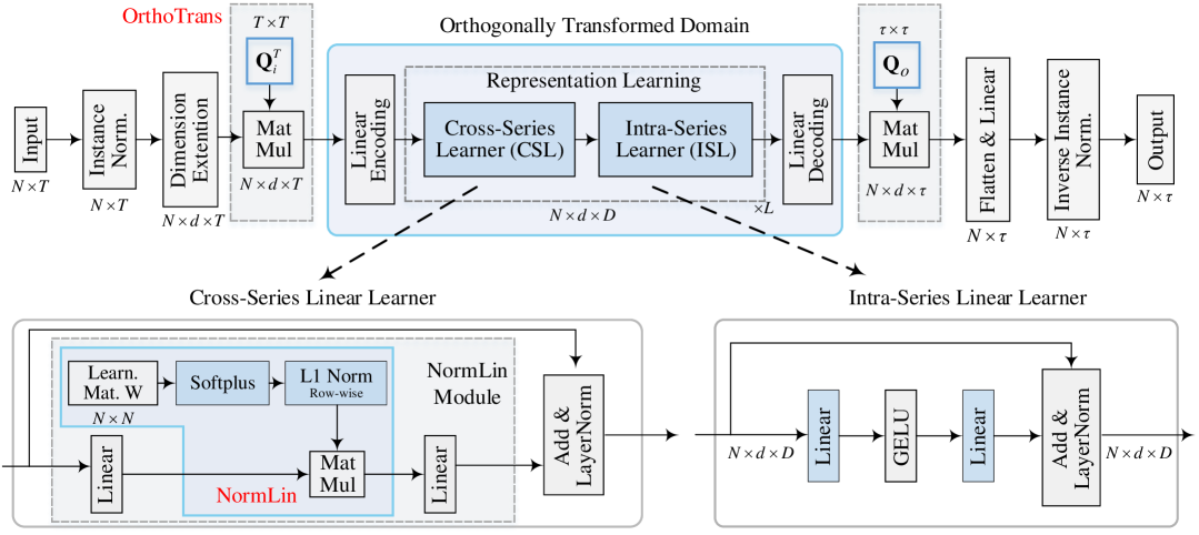
Figure 1: Overall structure of OLinear. The orthogonal matrix derived from the series’ temporal Pearson correlation matrix transforms the series into the new feature domain with removed sequential correlations. The cross-series learners and intra-series learners are then employed for robust representation learning. Specifically, we introduce the NormLin layer, whose weight matrix is processed by the Softplus function and row-wise L1 normalization, to capture multivariate correlations.

4 Method

Problem formulation

For multivariate time series forecasting, given a historical sequence $\mathbf{X}=\left\{\mathbf{x}_{1},\cdots,\mathbf{x}_{T}\right\}\in\mathbb{R}^{N\times T}$ with $T$ time steps and $N$ variates, the task is to predict the future $\tau$ time steps $\mathbf{Y}=\left\{\mathbf{x}_{T+1},\cdots,\mathbf{x}_{T+\tau}\right\}\in\mathbb{R}^{N\times\tau}$. Our goal is to approximate the ground truth $\mathbf{Y}$ as closely as possible with predictions $\hat{\mathbf{Y}}$.

4.1 Overall architecture

As shown in Figure 1, OLinear adopts a simple yet effective architecture. Given the input series $\mathbf{X}$, a RevIN (Kim et al., 2021) layer first performs instance normalization to mitigate non-stationarity. A dimension extension module then enhances expressiveness (Yi et al., 2023) by computing the outer product with a learnable vector $\phi_{d}\in\mathbb{R}^{d}$, where $d$ is the embedding size. Next, the time domain is decorrelated by multiplying with a transposed orthogonal matrix $\mathbf{Q}_{i}^{\mathsf{T}}\in\mathbb{R}^{T\times T}$, as detailed in Section 4.2. This process can be formulated as $\mathbf{Z}=\left(\mathrm{RevIN}_{\mathrm{Norm}}\left(\mathbf{X}\right)\otimes\phi_{d}\right)\cdot\mathbf{Q}_{i}^{\mathsf{T}}\in\mathbb{R}^{N\times d\times T}$, where $\otimes$ and $\cdot$ denote the outer product and standard matrix multiplication, respectively.

We then perform encoding and forecasting in the transformed domain. Specifically, a linear layer first encodes the decorrelated features $\mathbf{Z}$ to the model dimension $D$. The cross-series learner (CSL) and intra-series learner (ISL) subsequently capture multivariate correlations and model intra-series dynamics, respectively. After passing through $L$ stacked blocks, the representation is decoded to the desired prediction length $\tau$, and then mapped back to the time domain via multiplication with the orthogonal matrix $\mathbf{Q}_{o}$. The overall process is summarized as:

$$\tilde{\mathbf{H}}^{0} =\mathrm{LinearEncode}\left(\mathbf{Z}\right)\in\mathbb{R}^{N\times d\times D},$$ (2)

$$\tilde{\mathbf{H}}^{l+1} =\mathrm{ISL}\left(\mathrm{CSL}\left(\tilde{\mathbf{H}}^{l}\right)\right),\quad l=0,\cdots,L-1,$$

$$\tilde{\mathbf{Y}} =\mathrm{LinearDecode}\left(\tilde{\mathbf{H}}^{L}\right)\cdot\mathbf{Q}_{o}\in\mathbb{R}^{N\times d\times\tau}.$$

Figure 2: Comparison between the time and transformed domains. (1) The series exhibits strong consistency in the transformed domain, which is desirable for forecasting. (2) Sequence correlations are effectively reduced in the transformed domain. (3) Periodicity can be clearly reflected in the correlation matrix. (4) The new domain typically exhibits energy compaction, with only a few dominant dimensions. More cases are shown in Figure 7.

Finally, the flattened output is mapped to shape $N\times\tau$ via a linear layer, then de-normalized to yield the final prediction: $\hat{\mathbf{Y}}=\mathrm{RevIN}_{\mathrm{DeNorm}}\left(\mathrm{FlattenLinear}\left(\tilde{\mathbf{Y}}\right)\right)$.

4.2 Orthogonal transformation (OrthoTrans)

One effective approach for decorrelating the series is based on the Pearson correlation matrix. Let $\mathbf{X}^{train}\in\mathbb{R}^{N\times M}$ denote the training set, where $M$ is the length of the training series. For each variate $j$, we generate $T$ lagged series with temporal offsets from $0$ to $T-1$: $\mathbf{s}_{i}^{j}=\mathbf{X}\left[j,\ i:M-T+i\right],\ i=0,\cdots T-1,$ where $\mathbf{s}_{i}^{j}$ denotes the $i$-th temporally lagged series of variate $j$. We then compute the Pearson correlation matrix $\mathrm{CorrMat}_{t}^{j}$ of $\{\mathbf{s}_{i}^{j}\}$, whose $(p,q)$-th entry is $\frac{\mathrm{Cov}\left(\mathbf{s}_{p},\mathbf{s}_{q}\right)}{\sqrt{\mathrm{Var}\left(\mathbf{s}_{p}\right)\cdot\mathrm{Var}\left(\mathbf{s}_{q}\right)}},\ p,q\in\left\{0,\cdots,T-1\right\}$.

Here, $\mathrm{Cov}(\cdot)$ denotes the covariance of two series, and $\mathrm{Var}(\cdot)$ denotes the variance. The final Pearson correlation matrix is then obtained by averaging over all variates: $\mathrm{CorrMat}_{t}=\frac{1}{N}\sum_{j=0}^{N-1}\mathrm{CorrMat}_{t}^{j}$.

Following the above procedure, the resulting $\mathrm{CorrMat}_{t}$ is symmetric with all diagonal entries equal to 1. Based on the properties of symmetric matrices, we perform eigenvalue decomposition as $\mathrm{CorrMat}_{t}=\mathbf{Q}_{i}\Lambda\mathbf{Q}_{i}^{\mathsf{T}}$, where $\mathbf{Q}_{i}$ is an orthogonal matrix (Horn and Johnson, 2012) whose columns are the eigenvectors of $\mathrm{CorrMat}_{t}$, and $\Lambda$ is a diagonal matrix containing the corresponding eigenvalues.

For the input series $\mathbf{x}$ with temporal correlation matrix $\mathrm{CorrMat}_{t}$ and unit variance, the covariance matrix of the transformed vector $\mathbf{Q}_{i}^{\mathsf{T}}\mathbf{x}$ is $\mathrm{CovMat}\left(\mathbf{Q}_{i}^{\mathsf{T}}\mathbf{x}\right)=\mathbf{Q}_{i}^{\mathsf{T}}\mathrm{CorrMat}_{t}\mathbf{Q}_{i}=\mathbf{Q}_{i}^{\mathsf{T}}\mathbf{Q}_{i}\Lambda\mathbf{Q}_{i}^{\mathsf{T}}\mathbf{Q}_{i}=\Lambda$, which is a diagonal matrix. Therefore, the entries of $\mathbf{Q}_{i}^{\mathsf{T}}\mathbf{x}$ are linearly independent, removing sequential dependencies. Similarly, we can compute $\mathbf{Q}_{o}\in\mathbb{R}^{\tau\times\tau}$, and recover the temporal correlations by multiplying with $\mathbf{Q}_{o}$. Note that $\mathbf{Q}_{i}$ and $\mathbf{Q}_{o}$ are pre-computed and used throughout training and inference. Ablation studies on these two matrices are discussed in Appendix J.3. Moreover, as shown in Appendix I.8, OLinear remains robust even when the orthogonal matrices $\mathbf{Q}_{i}$ and $\mathbf{Q}_{o}$ are computed with limited training data.

Discussion

(1) Mathematically, $\mathbf{Q}_{i}^{\mathsf{T}}\mathbf{x}$ projects $\mathbf{x}$ onto the eigenvectors of the temporal correlation matrix $\mathrm{CorrMat}_{t}$. The transformed domain exhibits energy compaction, and noise is suppressed in the primary components (Bishop and Nasrabadi, 2006). (2) Compared to DFT and wavelet transforms, or to the TF paradigm without any transformation, OrthoTrans produces higher-rank attention matrices for Transformer-based forecasters (see Figures 10– 14), indicating greater representation diversity and enhanced model expressiveness. This partly explains why OrthoTrans enhances other forecasters when used as a plug-in module.

4.3 Representation learning

CSL and NormLin

Inspired by the properties of attention matrices in self-attention (Vaswani et al., 2017), we impose two constraints on the weight matrix of the linear layer for robust multivariate representation learning: (1) all entries must be positive, and (2) each row must sum to 1. To enforce these constraints, we apply the Softplus function followed by row-wise L1 normalization to the learnable weight matrix $\mathbf{W}$. The resulting layer is referred to as NormLin, and is defined as follows:

$$\mathrm{NormLin}\left(\mathbf{x}\right)=\mathrm{RowNorm}_{\mathrm{L1}}\left(\mathrm{Softplus}\left(\mathbf{W}\right)\right)\ \mathbf{x},\mathbf{W}\in\mathbb{R}^{N\times N},\mathbf{x}\in\mathbb{R}^{N}.$$ (3)

The variants of NormLin are discussed in Appendix J.1. Incorporating the other components in Figure 1(b), the CSL process is formulated as:

$$\mathrm{CSL}\left(\tilde{\mathbf{H}}\right)=\mathrm{LayerNorm}\left(\tilde{\mathbf{H}}+\mathrm{Linear}\left(\mathrm{NormLin}\left(\mathrm{Linear}\left(\tilde{\mathbf{H}}\right)\right)\right)\right),$$ (4)

Table 1: Comparison of FLOPs and memory usage between the NormLin module and multi-head self-attention (MHSA). Here, $h$ denotes the number of attention heads, typically set to 8.

Module	NormLin Module	MHSA
FLOPs	$\mathcal{O}\left(N^{2}D+2ND^{2}\right)$	$\mathcal{O}\left(2N^{2}D+4ND^{2}\right)$
Memory	$\mathcal{O}\left(N^{2}+ND\right)$	$\mathcal{O}\left(hN^{2}+ND\right)$

where $\mathrm{Linear}(\cdot)$ and $\mathrm{NormLin}(\cdot)$ operate on the sequence and variate dimensions, respectively. We define the NormLin module as $\mathrm{NormLinModule}\left(\cdot\right)\triangleq\mathrm{Linear}\left(\mathrm{NormLin}\left(\mathrm{Linear}\left(\cdot\right)\right)\right)$. Ablation studies on the two linear layers in $\mathrm{NormLinModule}\left(\cdot\right)$ are presented in Appendix J.2.

ISL

We adopt two linear layers separated by the GELU activation function as a powerful predictive representation learner (Li et al., 2023). It has been well established that MLPs are highly effective for encoding sequential dynamics and decoding future series (Zeng et al., 2023; Das et al., 2023). Similar to CSL, residual connections and LayerNorm are also applied. The complete ISL process is defined as:

$$\mathrm{ISL}\left(\tilde{\mathbf{H}}\right)=\mathrm{LayerNorm}\left(\tilde{\mathbf{H}}+\mathrm{Linear}\left(\mathrm{GELU}\left(\mathrm{Linear}\left(\tilde{\mathbf{H}}\right)\right)\right)\right).$$ (5)

Discussion

Compared to the self-attention mechanism, the NormLin module offers three main advantages: (1) As shown in Table 1, it reduces computational complexity by half and decreases memory footprint by a factor of $1/h$, where $h$ is the number of attention heads; (2) The learned weight matrix in NormLin naturally exhibits high rank, in contrast to the low-rank nature of self-attention (see Appendix E.2). The low-rank issue in self-attention could arise from the sharp value concentration of the Softmax function. A higher-rank weight (or attention) matrix often better preserves the rank of the representation space and thus improves the model’s expressiveness (Han et al., 2023). (3) From the perspective of gradient flow, the NormLin layer provides a more direct backpropagation path for optimizing weight entries. Appendix B shows that the Jacobian matrices of $\mathrm{Softmax}(\cdot)$ in self-attention and $\mathrm{Norm}_{\mathrm{L1}}(\mathrm{Softplus}(\cdot))$ in the NormLin layer share a similar structure, but the latter offers greater flexibility. As illustrated in Figure 6, the Jacobian matrix of NormLin typically contains more large-magnitude entries, indicating stronger and more effective gradient propagation during training.

5 Experiments

Datasets and implementation details

We extensively evaluate OLinear using 24 diverse real-world datasets: ETT (four subsets), Weather, ECL, Traffic, Exchange, Solar-Energy, PEMS (four subsets), ILI, COVID-19, METR-LA, NASDAQ, Wiki, SP500, DowJones, CarSales, Power, Website, Unemp. The weighted L1 loss function from CARD (Wang et al., 2024b) is adopted. The embedding size $d$ is set as 16. Dataset description and more implementation details are presented in Appendices C and D, respectively.

5.1 Forecasting performance

Baselines

We carefully choose 11 well-acknowledged state-of-the-art forecasting models as our baselines, including (1) Linear-based models: TimeMixer (Wang et al., 2024a), FilterNet (Yi et al., 2024a), FITS (Xu et al., 2024), DLinear (Zeng et al., 2023); (2) Transformer-based models: TimeMixer++ (Wang et al., 2025a), Leddam (Yu et al., 2024), CARD (Wang et al., 2024b), Fredformer (Piao et al., 2024), iTransformer (Liu et al., 2024a), PatchTST (Nie et al., 2023); (3) TCN-based model: TimesNet (Wu et al., 2023b).

Table 2: Long-term forecasting results with prediction lengths $\tau\in\left\{12,24,48,96\right\}$ for PEMS and $\tau\in\left\{96,192,336,720\right\}$ for others. Lookback horizon $T=96$. Results are averaged over four prediction lengths. Avg denotes further averaging over subsets. Full results are shown in Table 15.

Model	OLinear (Ours)		TimeMix. 2024a		FilterNet 2024a		DLinear 2023		TimeMix.++ 2025a		Leddam 2024		CARD 2024b		Fredformer 2024		iTrans. 2024a		PatchTST 2023		TimesNet 2023b
Metric	MSE	MAE	MSE	MAE	MSE	MAE	MSE	MAE	MSE	MAE	MSE	MAE	MSE	MAE	MSE	MAE	MSE	MAE	MSE	MAE	MSE	MAE
ETT(Avg)	0.359	0.376	0.367	0.388	0.375	0.394	0.442	0.444	0.349	0.377	0.367	0.387	0.366	0.380	0.366	0.385	0.383	0.399	0.380	0.396	0.391	0.404
ECL	0.159	0.248	0.182	0.273	0.173	0.268	0.212	0.300	0.165	0.253	0.169	0.263	0.168	0.258	0.176	0.269	0.178	0.270	0.208	0.295	0.192	0.295
Exchange	0.355	0.399	0.387	0.416	0.388	0.419	0.354	0.414	0.357	0.409	0.354	0.402	0.362	0.402	0.333	0.391	0.360	0.403	0.367	0.404	0.416	0.443
Traffic	0.451	0.247	0.485	0.298	0.463	0.310	0.625	0.383	0.416	0.264	0.467	0.294	0.453	0.282	0.433	0.291	0.428	0.282	0.531	0.343	0.620	0.336
Weather	0.237	0.260	0.240	0.272	0.245	0.272	0.265	0.317	0.226	0.262	0.242	0.272	0.239	0.265	0.246	0.272	0.258	0.279	0.259	0.281	0.259	0.287
Solar	0.215	0.217	0.216	0.280	0.235	0.266	0.330	0.401	0.203	0.258	0.230	0.264	0.237	0.237	0.226	0.262	0.233	0.262	0.270	0.307	0.301	0.319
PEMS03	0.095	0.199	0.167	0.267	0.145	0.251	0.278	0.375	0.165	0.263	0.107	0.210	0.174	0.275	0.135	0.243	0.113	0.221	0.180	0.291	0.147	0.248
PEMS04	0.091	0.190	0.185	0.287	0.146	0.258	0.295	0.388	0.136	0.251	0.103	0.210	0.206	0.299	0.162	0.261	0.111	0.221	0.195	0.307	0.129	0.241
PEMS07	0.077	0.164	0.181	0.271	0.123	0.229	0.329	0.395	0.152	0.258	0.084	0.180	0.149	0.247	0.121	0.222	0.101	0.204	0.211	0.303	0.124	0.225
PEMS08	0.113	0.194	0.226	0.299	0.172	0.260	0.379	0.416	0.200	0.279	0.122	0.211	0.201	0.280	0.161	0.250	0.150	0.226	0.280	0.321	0.193	0.271
1st Count	5	9	0	0	0	0	0	0	4	0	0	0	0	0	1	1	0	0	0	0	0	0

Table 3: Short-term forecasting results. Two settings are applied: S1 (Input-12, Predict-$\left\{3,6,9,12\right\}$) and S2 (Input-36, Predict-$\left\{24,36,48,60\right\}$). Average results across eight prediction lengths are reported. Full results are provided in Tables 16 and 17.

Model	OLinear (Ours)		TimeMix. 2024a		FilterNet 2024a		DLinear 2023		TimeMix.++ 2025a		Leddam 2024		CARD 2024b		Fredformer 2024		iTrans. 2024a		PatchTST 2023		TimesNet 2023b
Metric	MSE	MAE	MSE	MAE	MSE	MAE	MSE	MAE	MSE	MAE	MSE	MAE	MSE	MAE	MSE	MAE	MSE	MAE	MSE	MAE	MSE	MAE
ILI	1.429	0.690	1.864	0.806	1.793	0.791	2.742	1.126	1.805	0.793	1.725	0.777	1.959	0.822	1.732	0.797	1.715	0.773	1.905	0.804	1.809	0.807
COVID-19	5.187	1.211	5.919	1.350	5.607	1.322	8.279	1.601	5.974	1.369	5.251	1.285	5.536	1.314	5.279	1.287	5.301	1.293	5.836	1.362	6.106	1.369
METR-LA	0.587	0.311	0.608	0.372	0.603	0.366	0.580	0.422	0.567	0.363	0.603	0.367	0.639	0.350	0.617	0.369	0.627	0.373	0.614	0.372	0.617	0.370
NASDAQ	0.121	0.201	0.120	0.204	0.127	0.211	0.150	0.251	0.125	0.210	0.128	0.211	0.125	0.207	0.127	0.210	0.133	0.217	0.128	0.209	0.161	0.247
Wiki	6.395	0.415	6.443	0.439	6.457	0.439	6.420	0.510	6.430	0.443	6.417	0.433	6.419	0.427	6.318	0.429	6.422	0.432	6.368	0.424	7.633	0.572
SP500	0.146	0.250	0.153	0.265	0.164	0.279	0.178	0.298	0.157	0.270	0.163	0.282	0.147	0.252	0.167	0.286	0.161	0.279	0.159	0.277	0.150	0.262
DowJones	7.686	0.619	8.499	0.633	8.283	0.633	7.893	0.626	8.895	0.643	8.257	0.633	7.699	0.619	8.041	0.625	8.177	0.630	7.991	0.626	10.960	0.737
CarSales	0.330	0.305	0.333	0.322	0.328	0.319	0.387	0.376	0.337	0.321	0.335	0.322	0.347	0.324	0.335	0.325	0.311	0.307	0.327	0.318	0.334	0.328
Power	1.248	0.835	1.234	0.840	1.309	0.870	1.278	0.870	1.234	0.841	1.295	0.868	1.288	0.847	1.302	0.870	1.324	0.874	1.311	0.873	1.317	0.871
Website	0.225	0.311	0.279	0.358	0.297	0.367	0.302	0.389	0.260	0.344	0.264	0.348	0.303	0.366	0.266	0.351	0.179	0.297	0.284	0.362	0.251	0.341
Unemp	0.729	0.461	1.581	0.708	1.286	0.627	0.565	0.509	1.506	0.678	1.502	0.689	1.163	0.596	2.048	0.789	1.408	0.666	1.237	0.624	2.328	0.852
1st Count	4	10	2	0	0	0	1	0	2	0	0	0	0	1	1	0	2	1	0	0	0	0

Main results

Comprehensive long-term and short-term forecasting results are presented in Tables 2 and 3, respectively, with the best results highlighted in bold and the second-best underlined. Lower MSE/MAE values indicate more accurate predictions. Across a wide range of benchmarks, OLinear consistently outperforms state-of-the-art Transformer-based and linear-based forecasters. Notably, these gains are achieved with high computational efficiency. (Figure 3 and Table 37).

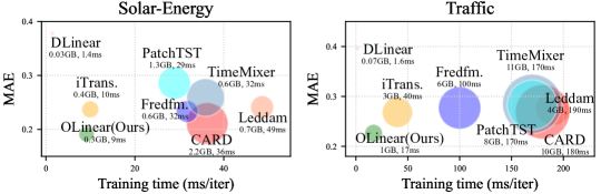
Figure 3: Model efficiency comparison. Bubble areas represent GPU memory usage during training, scaled independently in the two subfigures. Resource footprint data are from Table 37.

We attribute this superior performance to the adopted OrthoTrans and NormLin modules. The effectiveness of the simpler NormLin module challenges the necessity of the widely adopted multi-head self-attention mechanism, which has been a dominant design in prior works. To further validate robustness, we evaluate OLinear under varying lookback lengths (Table 26), where it consistently outperforms existing state-of-the-art methods.

Figure 4 shows the prediction visualizations of OLinear. Moreover, Table 13 demonstrates that OLinear exhibits greater robustness to random seeds compared to state-of-the-art Transformer-based forecasters such as TimeMixer++ and iTransformer.

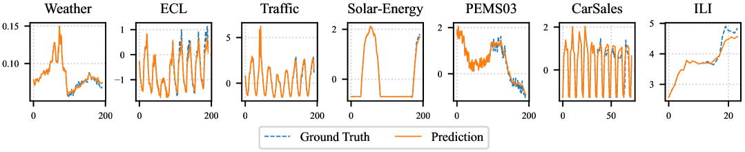
Figure 4: Visualization of the forecasting results of OLinear, demonstrating great accuracy.

Table 4: Ablation study on transformation bases. S1 and S2 represent ‘Input-12, Predict-$\{3,6,9,12\}$’ and ‘Input-36, Predict-$\{24,36,48,60\}$’, respectively. Wavelet1 and Wavelet2 use the Haar and discrete Meyer wavelets. Identity denotes no transformation. Full results are in Table 18.

Dataset	ECL		Solar-Energy		PEMS03		Power (S2)		ILI (S1)		COVID (S2)		METR-LA (S2)
Metric	MSE	MAE	MSE	MAE	MSE	MAE	MSE	MAE	MSE	MAE	MSE	MAE	MSE	MAE
Ours	0.159	0.248	0.215	0.217	0.095	0.199	1.487	0.922	1.094	0.578	8.467	1.754	0.838	0.402
Fourier	0.161	0.250	0.219	0.219	0.101	0.204	1.614	0.967	1.268	0.584	9.165	1.839	0.843	0.403
Wavelet1	0.160	0.249	0.221	0.221	0.107	0.210	1.663	0.987	0.116	0.580	8.666	1.799	0.840	0.404
Wavelet2	0.162	0.251	0.226	0.224	0.108	0.210	1.664	0.987	1.177	0.594	8.949	1.840	0.843	0.406
Chebyshev	0.218	0.295	0.226	0.226	0.105	0.207	1.570	0.965	1.217	0.597	9.330	1.875	0.854	0.407
Laguerre	0.167	0.255	0.233	0.230	0.111	0.214	1.659	0.984	1.353	0.651	9.302	1.890	0.868	0.420
Legendre	0.161	0.250	0.243	0.235	0.109	0.213	1.685	0.995	1.177	0.603	8.550	1.798	0.841	0.404
Identity	0.163	0.252	0.227	0.225	0.106	0.209	1.542	0.945	1.153	0.587	8.856	1.819	0.848	0.408

5.2 Model analysis

Transformation bases

We replace OrthoTrans with several commonly used bases, including the Fourier basis, two wavelet bases (Haar and discrete Meyer wavelets), and three polynomial bases. As shown in Table 4, our method consistently outperforms all alternatives. Specifically, it achieves a 5.5% reduction in MSE over the Fourier basis, and a 10.0% improvement over the no-transformation baseline (i.e., the TF paradigm) on PEMS03.

OrthoTrans as a plug-in

We further integrate OrthoTrans into three classic forecasters: iTransformer, PatchTST, and RLinear (Li et al., 2023). As shown in Table 5, OrthoTrans yields average MSE improvements of 5.1% and 10.1% for iTransformer and PatchTST, respectively, highlighting the benefit of incorporating dataset-specific statistical information into the model design. This improvement can be attributed to the increased attention matrix rank introduced by OrthoTrans (see Appendix E.3), which indicates enlarged representation space and enhanced model capacity (Han et al., 2023).

Table 5: Applying OrthoTrans (O.Trans) to iTransformer, PatchTST and RLinear. Average MSEs are reported. Full results are in Table 19.

Model	iTrans. 2024a		PatchTST 2023		RLinear 2023
	Van.	+O.Trans	Van.	+O.Trans	Van.	+O.Trans
ETTm1	0.407	0.404	0.387	0.384	0.414	0.408
ECL	0.178	0.171	0.208	0.181	0.219	0.214
PEMS03	0.113	0.103	0.180	0.163	0.495	0.477
PEMS07	0.101	0.085	0.211	0.147	0.504	0.485
Solar	0.233	0.228	0.270	0.239	0.369	0.354
Weather	0.258	0.252	0.259	0.246	0.272	0.269
METR-LA	0.338	0.329	0.335	0.333	0.342	0.341

Representation learning

To validate the rationality of our CSL and ISL designs, we conduct ablation studies by replacing or removing their core components—NormLin and (standard) linear layers. As shown in Table 6, our design—applying NormLin along the variate dimension and standard linear layers along the temporal dimension—consistently achieves the best performance. Notably, applying NormLin along the variate dimension consistently outperforms its self-attention counterpart (last row), with reduced computational cost. Furthermore, removing the ISL module (third-last row) results in a 6.2% performance decline, highlighting the importance of updating temporal representations. Interestingly, on small-scale datasets with fewer variates (e.g., NASDAQ and ILI), the model with only temporal linear layers (third row) exhibits competitive performance, implying that NormLin is more beneficial when handling a larger number of variates.

Table 6: Ablations on the CSL and ISL design. ‘NormLin (Temporal)’ replaces the linear layer in Eq. 5 with the NormLin layer, and ‘Linear (Variate)’ replaces the NormLin layer in Eq. 4 with a standard linear layer. ‘Attn.’ denotes the self-attention mechanism. Results are averaged over four prediction lengths. Full results are shown in Table 20.

		ECL		Traffic		Solar		PEMS03		Weather		ETTm1		NASDAQ (S1)		ILI (S2)
Variate	Temp.	MSE	MAE	MSE	MAE	MSE	MAE	MSE	MAE	MSE	MAE	MSE	MAE	MSE	MAE	MSE	MAE
NormLin	Linear	0.159	0.248	0.451	0.247	0.215	0.217	0.095	0.199	0.237	0.260	0.374	0.377	0.055	0.125	1.764	0.802
Linear	Linear	0.178	0.272	0.606	0.320	0.246	0.238	0.121	0.226	0.238	0.261	0.377	0.380	0.057	0.132	1.938	0.837
w/o	Linear	0.178	0.259	0.482	0.257	0.241	0.232	0.147	0.234	0.247	0.266	0.378	0.379	0.054	0.124	1.864	0.823
NormLin	NormLin	0.169	0.257	0.460	0.275	0.252	0.240	0.112	0.214	0.239	0.261	0.381	0.382	0.055	0.126	1.947	0.836
Linear	NormLin	0.183	0.276	0.578	0.339	0.262	0.254	0.143	0.246	0.240	0.261	0.383	0.384	0.057	0.133	2.037	0.867
w/o	NormLin	0.185	0.266	0.493	0.290	0.283	0.262	0.182	0.269	0.246	0.265	0.384	0.385	0.055	0.125	2.093	0.874
NormLin	w/o	0.169	0.257	0.460	0.275	0.253	0.241	0.114	0.215	0.239	0.261	0.380	0.382	0.055	0.126	1.940	0.837
Linear	w/o	0.183	0.276	0.591	0.341	0.262	0.254	0.142	0.246	0.240	0.262	0.384	0.384	0.057	0.132	2.073	0.874
Attn.	Linear	0.166	0.255	0.457	0.251	0.220	0.221	0.097	0.202	0.244	0.265	0.391	0.389	0.056	0.126	2.022	0.847

OLinear-C

As shown in Figure 5, the learned weight matrix resemble $\mathrm{Softmax}\left(\mathrm{CorrMat}_{v}\right)$, where $\mathrm{CorrMat}_{v}$ is the Pearson correlation matrix across variates. Motivated by this, we replace the learnable weights in NormLin with the pre-computed $\mathrm{Softmax}\left(\mathrm{CorrMat}_{v}\right)$, resulting in a simplified variant: $\mathrm{NormLin}_{c}\left(\mathbf{x}\right)=\mathrm{Softmax}\left(\mathrm{CorrMat}_{v}\right)\ \mathbf{x}$. We refer to the model with this NormLin variant as OLinear-C.

Table 7: Performance comparison of OLinear and OLinear-C. Full results are shown in Table 23.

Dataset	ECL		Traffic		ETT		Solar		PEMS		CarSales		ILI		COVID-19		Unemp
Metric	MSE	MAE	MSE	MAE	MSE	MAE	MSE	MAE	MSE	MAE	MSE	MAE	MSE	MAE	MSE	MAE	MSE	MAE
OLinear	0.159	0.248	0.451	0.247	0.359	0.376	0.215	0.217	0.094	0.187	0.330	0.305	1.429	0.690	5.187	1.211	0.729	0.461
OLinear-C	0.161	0.249	0.451	0.247	0.359	0.376	0.215	0.217	0.094	0.187	0.330	0.305	1.463	0.698	5.346	1.247	0.766	0.474

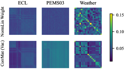
Figure 5: The learned NormLin weights exhibit similarity to the multivariate correlation matrix (after Softmax).

Table 7 shows that OLinear-C performs comparably to OLinear with reduced learnable parameters. Comprehensive evaluation of OLinear-C and the variants of $\mathrm{NormLin}_{c}$ are discussed in Appendix H.

5.3 Generality and scalability of the NormLin module

Table 8: Comparison of the NormLin module with state-of-the-art attention variants. Average MSEs are reported. Full results are in Table 21.

Dataset	NormLin (Ours)	Trans. 2017	Refm. 2020	Flowfm. 2022	Flatten 2023	Mamba 2023	E.Attn. 2025
ECL	0.159	0.166	0.167	0.165	0.164	0.176	0.159
Traffic	0.451	0.457	0.459	0.460	0.464	0.456	0.439
PEMS03	0.095	0.097	0.096	0.099	0.101	0.104	0.097
Weather	0.237	0.244	0.241	0.242	0.246	0.242	0.241
Solar	0.215	0.223	0.216	0.222	0.231	0.228	0.217
ILI	1.764	2.022	1.821	1.881	2.134	1.950	1.878
NASDAQ	0.055	0.056	0.055	0.055	0.057	0.055	0.055

Table 9: Applying NormLin (N.Lin) to state-of-the-art Transformer-based forecasters. Average MSEs are reported. Full results are in Table 22.

	iTrans.		PatchTST		Leddam		Fredformer
Dataset	Van.	N.Lin	Van.	N.Lin	Van.	N.Lin	Van.	N.Lin
ETTm1	0.407	0.388	0.387	0.379	0.386	0.381	0.384	0.381
ECL	0.178	0.166	0.208	0.181	0.169	0.165	0.176	0.169
PEMS03	0.113	0.102	0.180	0.146	0.107	0.103	0.134	0.108
PEMS07	0.101	0.086	0.211	0.168	0.084	0.082	0.121	0.096
Solar	0.233	0.226	0.270	0.237	0.230	0.222	0.226	0.226
Weather	0.258	0.245	0.259	0.245	0.242	0.242	0.246	0.240
METR-LA	0.338	0.328	0.335	0.333	0.327	0.320	0.336	0.329

In our CSL module, we employ the NormLin module—comprising the NormLin layer and its associated pre- and post-linear layers (Equation 4)—to capture multivariate correlations. Despite its simple architecture, the NormLin module demonstrates strong capability, generality, and scalability. Specifically, it consistently outperforms the classic multi-head self-attention mechanism and its variants, offering a compelling alternative for token dependency modeling.

Comparison with attention mechanisms

To assess its effectiveness, we compare NormLin with classic attention variants, such as Reformer (Kitaev et al., 2020), Flowformer (Wu et al., 2022), FLatten (Dao et al., 2022), and Mamba (Gu and Dao, 2023). As shown in Table 9, NormLin consistently outperforms these methods, demonstrating that the simple normalized weight matrix performs better than the complex query-key interaction mechanism for time series forecasting.

Table 10: Applying NormLin to the large time series model Timer. For fine-tuning, 5% samples of trainset are used. MSEs are reported.

Dataset	Fine-tuning		Zero-shot
	Van.	NormLin	Van.	NormLin
ETTh1	0.362	0.360	0.438	0.404
ETTh2	0.280	0.269	0.314	0.274
ETTm1	0.321	0.309	0.690	0.632
ETTm2	0.176	0.172	0.213	0.212
ECL	0.132	0.130	0.192	0.183
Traffic	0.361	0.353	0.458	0.462
Weather	0.151	0.149	0.181	0.174

NormLin as a plug-in

To demonstrate the generalizability of the NormLin module, we replace self-attention with NormLin in Transformer-based forecasters. As shown in Table 9, this substitution leads to notable MSE improvements—6.7% for iTransformer and 10.3% for PatchTST—validating its plug-and-play effectiveness. These results also validate NormLin’s capability to model dependencies across multiple token types (i.e., variate, temporal, and frequency-domain), highlighting its potential as a universal token dependency learner for time series forecasting. Furthermore, the NormLin module consistently improves both training and inference efficiency across these models (see Table 38); for example, it boosts iTransformer’s inference efficiency by an average of 53%.

Scalability of the NormLin module

Decoder-only Transformers have become the de facto architecture choice for large time series models (Liu et al., 2024b; Ansari et al., 2024; Das et al., 2024). We take Timer (Liu et al., 2024b) as a representative example and replace self-attention in Timer with NormLin. To align with Timer’s decoder-only structure, we apply a causal mask by zeroing out the upper triangular part of NormLin’s weight matrix. The modified model is pre-trained on the UTSD dataset (Liu et al., 2024b), which spans seven domains and contains up to 1 billion time points. As shown in Table 10, NormLin improves performance in both zero-shot and fine-tuning scenarios. For example, the zero-shot MSE on ETTh2 and ETTm1 is reduced by 12.7% and 8.4%, respectively. These results demonstrate that the NormLin module adapts well to decoder-only architectures and scales effectively to large-scale pre-training scenarios.

6 Conclusion

In this work, we present OLinear, a simple yet effective linear-based forecaster that achieves state-of-the-art performance, built on two core components: (1) OrthoTrans, an orthogonal transformation that decorrelates temporal dependencies to facilitate better encoding and forecasting, and (2) the NormLin module, a powerful and general-purpose token dependency learner. Notably, both modules consistently improve existing forecasters when used as plug-ins. In future work, we plan to apply the NormLin module to large time series models and broader time series analysis tasks.

Appendix A Proof of Theorem 1

Proof.

For clarity, we denote $\mathbf{z}\triangleq\begin{bmatrix}\mathbf{x}\\ y\end{bmatrix}\in\mathbb{R}^{t+1}$, $\mu_{z}\triangleq\begin{bmatrix}\mu_{\mathbf{x}}\\ \mu_{y}\end{bmatrix}\in\mathbb{R}^{t+1}$, and $\Sigma\triangleq\begin{bmatrix}\Sigma_{\mathbf{x}}&\Sigma_{\mathbf{x}y}\\ \Sigma_{\mathbf{x}y}^{\mathsf{T}}&\sigma_{y}^{2}\end{bmatrix}$. According to the definition, the probability density function of $\mathrm{z}$, i.e, the joint density of $\mathbf{x}$ and $y$, is

$$p(\mathbf{z})=p(\mathbf{x},y)=\frac{1}{(2\pi)^{(t+1)/2}|\Sigma|^{1/2}}\exp\left(-\frac{1}{2}(\mathbf{z}-\mu_{z})^{\mathsf{T}}\Sigma^{-1}(\mathbf{z}-\mu_{z})\right),$$ (6)

where $|\Sigma|$ denotes the determinant of $\Sigma$. In the following, we ignore the constant coefficient and focus on the exponential term.

Using the standard block matrix inverse formula [Horn and Johnson, 2012], we have

$$\Sigma^{-1}=\begin{bmatrix}\Sigma_{\mathbf{x}}^{-1}+d^{-1}\Sigma_{\mathbf{x}}^{-1}\Sigma_{\mathbf{x}y}\Sigma_{\mathbf{x}y}^{\mathsf{T}}\Sigma_{\mathbf{x}}^{-1}&-d^{-1}\Sigma_{\mathbf{x}}^{-1}\Sigma_{\mathbf{x}y}\\ -d^{-1}\Sigma_{\mathbf{x}y}^{\mathsf{T}}\Sigma_{\mathbf{x}}^{-1}&d^{-1}\end{bmatrix}\triangleq\begin{bmatrix}\mathbf{A}&-\mathbf{b}\\ -\mathbf{b}^{\mathsf{T}}&d^{-1}\end{bmatrix},$$ (7)

where the scalar $d=\sigma_{y}^{2}-\Sigma_{\mathbf{x}y}^{\mathsf{T}}\Sigma_{\mathbf{x}}^{-1}\Sigma_{\mathbf{x}y}$ is the Schur complement [Horn and Johnson, 2012]. Letting $\mathbf{b}\in\mathbb{R}^{t\times 1}$ denote $d^{-1}\Sigma_{\mathbf{x}}^{-1}\Sigma_{\mathbf{x}y}$, the matrix $\mathbf{A}$ becomes $\Sigma_{\mathbf{x}}^{-1}+d\cdot\mathbf{b}\mathbf{b}^{\mathsf{T}}$.

For notational simplicity, we define $\mathbf{\alpha}\triangleq\mathbf{x}-\mu_{\mathbf{x}}\in\mathbb{R}^{t\times 1}$ and $\beta\triangleq y-\mu_{y}\in\mathbb{R}$. Then, the exponent in Equation 6 (ignoring the constant factor $-1/2$) becomes

$$(\mathbf{z}-\mu_{z})^{\mathsf{T}}\Sigma^{-1}(\mathbf{z}-\mu_{z}) =\begin{bmatrix}\alpha^{\mathsf{T}}&\beta\end{bmatrix}\begin{bmatrix}\Sigma_{\mathbf{x}}^{-1}+d\cdot\mathbf{b}\mathbf{b}^{\mathsf{T}}&-\mathbf{b}\\ -\mathbf{b}^{\mathsf{T}}&d^{-1}\end{bmatrix}\begin{bmatrix}\alpha\\ \beta\end{bmatrix}$$ (8)

$$=\alpha^{\mathsf{T}}\Sigma_{\mathbf{x}}^{-1}\alpha+d\cdot\alpha^{\mathsf{T}}\mathbf{b}\mathbf{b}^{\mathsf{T}}-2\beta\alpha^{\mathsf{T}}\mathbf{b}+d^{-1}\beta^{2}$$

$$=\alpha^{\mathsf{T}}\Sigma_{\mathbf{x}}^{-1}\alpha+d^{-1}\left(\beta^{2}-2d\cdot\alpha^{\mathsf{T}}\mathbf{b}\cdot\beta+d^{2}\cdot\alpha^{\mathsf{T}}\mathbf{b}\mathbf{b}^{\mathsf{T}}\alpha\right)$$

$$=\alpha^{\mathsf{T}}\Sigma_{\mathbf{x}}^{-1}\alpha+d^{-1}\left(\beta-d\alpha^{\mathsf{T}}\mathbf{b}\right)^{2}.$$

Since $p(\mathbf{x})\propto\exp\left(-\frac{1}{2}\alpha^{\mathsf{T}}\Sigma_{\mathbf{x}}^{-1}\alpha\right)$, it follows that

$$p(y\mid\mathbf{x}) =\frac{p(\mathbf{x},y)}{p(\mathbf{x})}$$ (9)

$$\propto\exp\left(-\frac{1}{2}\left(\alpha^{\mathsf{T}}\Sigma_{\mathbf{x}}^{-1}\alpha+d^{-1}\left(\beta-d\alpha^{\mathsf{T}}\mathbf{b}\right)^{2}-\alpha^{\mathsf{T}}\Sigma_{x}^{-1}\alpha\right)\right)$$

$$=\exp\left(-\frac{\left(\beta-d\alpha^{\mathsf{T}}\mathbf{b}\right)^{2}}{2d}\right)$$

$$=\exp\left(-\frac{\left(y-\mu_{y}-d\alpha^{\mathsf{T}}\mathbf{b}\right)^{2}}{2d}\right).$$

Therefore, the conditional density of $y$ give $\mathbf{x}$ is also a Gaussian distribution, whose mean is

$$\mu_{y}+d\alpha^{\mathsf{T}}\mathbf{b} =\mu_{y}+d\mathbf{b}^{\mathsf{T}}\alpha$$ (10)

$$=\mu_{y}+d\cdot d^{-1}\Sigma_{\mathbf{x}y}^{\mathsf{T}}\Sigma_{\mathbf{x}}^{-1}\left(\mathbf{x}-\mu_{x}\right)$$

$$=\mu_{y}+\Sigma_{\mathbf{x}y}^{\mathsf{T}}\Sigma_{\mathbf{x}}^{-1}\left(\mathbf{x}-\mu_{\mathbf{x}}\right),$$

and the variance is $d=\sigma_{y}^{2}-\Sigma_{\mathbf{x}y}^{\mathsf{T}}\Sigma_{\mathbf{x}}^{-1}\Sigma_{\mathbf{x}y}$. This completes the proof.

∎

Appendix B Jacobian matrix comparison of self-attention and NormLin

In this section, we analyze the gradients of the non-linear transformations in the self-attention mechanism and the NormLin module, focusing on the attention/weight rows, denoted as $\mathbf{a}\in\mathbb{R}^{N}$.

B.1 Jacobian matrix of Softmax in self-attention

Let $\mathbf{c}\triangleq\mathrm{Softmax}(\mathbf{a})\in\mathbb{R}^{N}$. We first compute the partial derivatives element-wise, and then rewrite the results in matrix form. Based on the definition of $\mathrm{Softmax}$, the $i$-th element of $\mathbf{c}$ is $\mathbf{c}_{i}=\frac{e^{\mathbf{a}_{i}}}{\sum_{k=1}^{N}e^{\mathbf{a}_{k}}}$. The partial derivative of $\mathbf{c}_{i}$ with respect to $\mathbf{a}_{i}$ is:

$$\frac{\partial\mathbf{c}_{i}}{\partial\mathbf{a}_{i}}=\frac{e^{\mathbf{a}_{i}}}{\sum_{k=1}^{N}e^{\mathbf{a}_{k}}}-\frac{e^{\mathbf{a}_{i}}\cdot e^{\mathbf{a}_{i}}}{(\sum_{k=1}^{N}e^{\mathbf{a}_{k}})^{2}}=\mathbf{c}_{i}-\mathbf{c}_{i}^{2}.$$ (11)

For $j\neq i$, the partial derivative of $\mathbf{c}_{i}$ with respect to $\mathbf{a}_{j}$ is:

$$\frac{\partial\mathbf{c}_{i}}{\partial\mathbf{a}_{j}}=-\frac{e^{\mathbf{a}_{i}}\cdot e^{\mathbf{a}_{j}}}{(\sum_{k=1}^{N}e^{\mathbf{a}_{k}})^{2}}=-\mathbf{c}_{i}\mathbf{c}_{j}$$ (12)

Combining Equations (11) and (12), we obtain:

$$\frac{\partial\mathbf{c}_{i}}{\partial\mathbf{a}}=\mathbf{c}_{i}[\delta_{1i},\delta_{2i},\ldots,\delta_{Ni}]-\mathbf{c}_{i}\mathbf{c}^{\mathsf{T}},$$ (13)

where $\delta_{ji}=1$ if $j=i$, otherwise 0. Therefore, the Jacobian matrix $\frac{\partial\mathbf{c}}{\partial\mathbf{a}}$ can be written as

$$\frac{\partial\mathbf{c}}{\partial\mathbf{a}}=\mathrm{Diag}(\mathbf{c})-\mathbf{c}\mathbf{c}^{\mathsf{T}},$$ (14)

where $\mathrm{Diag}(\mathbf{c})$ is the diagonal matrix with $\mathbf{c}$ as its diagonal. We can observe that the Jacobian matrix is a function of $\mathbf{c}$. Since the Softmax function could cause sharp value concentration, the Jacobian matrix may exhibit sparsity, with most entries being close to zero [Surya Duvvuri and Dhillon, 2024].

B.2 Jacobian matrix of the NormLin layer

Let $\mathbf{c}\triangleq\mathrm{Norm}_{\mathrm{L1}}\left(\mathrm{Softplus}\left(\mathbf{a}\right)\right)\in\mathbb{R}^{N}$, where $\mathrm{Norm}_{\mathrm{L1}}(\cdot)$ denotes the L1 normalization. For notational simplicity, let $\mathbf{b}\triangleq\mathrm{Softplus}(\mathbf{a})$. We first analyze $\frac{\partial\mathbf{c}}{\partial\mathbf{b}}$. Since all entries of $\mathbf{b}$ are positive, we have:

$$\mathbf{c}_{i}=\frac{\mathbf{b}_{i}}{\sum_{k=1}^{N}\mathbf{b}_{k}}.$$ (15)

Therefore, it follows that

$$\frac{\partial\mathbf{c}_{i}}{\partial\mathbf{b}_{i}}=\frac{1}{\sum_{k=1}^{N}\mathbf{b}_{k}}-\frac{\mathbf{b}_{i}}{(\sum_{k=1}^{N}\mathbf{b}_{k})^{2}}=\frac{1}{\left\|\mathbf{b}\right\|_{1}^{2}}\left(\left\|\mathbf{b}\right\|_{1}-\mathbf{b}_{i}\right).$$ (16)

For $j\neq i$, the partial derivative $\frac{\partial\mathbf{c}_{i}}{\partial\mathbf{b}_{j}}$ is:

$$\frac{\partial\mathbf{c}_{i}}{\partial\mathbf{b}_{j}}=-\frac{\mathbf{b}_{i}}{(\sum_{k=1}^{N}\mathbf{b}_{k})^{2}}=-\frac{1}{\left\|\mathbf{b}\right\|_{1}^{2}}\mathbf{b}_{i}.$$ (17)

Combining Equations (16) and (17), we obtain the Jacobian matrix:

$$\frac{\partial\mathbf{c}}{\partial\mathbf{b}}=\frac{1}{\left\|\mathbf{b}\right\|_{1}^{2}}\left(\left\|\mathbf{b}\right\|_{1}\mathbf{I}-\mathbf{b}\mathbf{1}^{\mathsf{T}}\right),$$ (18)

where $\mathbf{1}\in\mathbb{R}^{N}$ is the all-ones vector.

For the derivative of $\mathbf{b}_{i}$ with respect to $\mathbf{a}_{j}$ with $1\leq i,j\leq N$, we have

$$\frac{\partial\mathbf{b}_{i}}{\partial\mathbf{a}_{j}} =\delta_{ij}\cdot\frac{\partial\mathbf{b}_{i}}{\partial\mathbf{a}_{i}}=\delta_{ij}\cdot\frac{\partial}{\partial\mathbf{a}_{i}}\mathrm{In}(1+e^{\mathbf{a}_{i}})$$ (19)

$$=\delta_{ij}\cdot\frac{e^{\mathbf{a}_{i}}}{1+e^{\mathbf{a}_{i}}}=\delta_{ij}\cdot\mathrm{Sigmoid}(\mathbf{a}_{i}).$$

Therefore, $\frac{\partial\mathbf{b}}{\partial\mathbf{a}}$ can be written as

$$\frac{\partial\mathbf{b}}{\partial\mathbf{a}}=\mathrm{Diag}\left(\mathrm{Sigmoid}(\mathbf{a})\right)\triangleq\mathrm{Diag}\left(\tilde{\mathbf{b}}\right),$$ (20)

where $\mathrm{Sigmoid}(\cdot)$ operates element-wise, and $\tilde{\mathbf{b}}\triangleq\mathrm{Sigmoid}(\mathbf{a})$ is defined for clarity. Using the chain rule, the Jacobian matrix of $\mathbf{c}$ with respect to $\mathbf{a}$ can be derived as follows:

$$\frac{\partial\mathbf{c}}{\partial\mathbf{a}} =\frac{\partial\mathbf{c}}{\partial\mathbf{b}}\cdot\frac{\partial\mathbf{b}}{\partial\mathbf{a}}=\frac{1}{\left\|\mathbf{b}\right\|_{1}^{2}}\left(\left\|\mathbf{b}\right\|_{1}\mathbf{I}-\mathbf{b}\mathbf{1}^{\mathsf{T}}\right)\mathrm{Diag}\left(\tilde{\mathbf{b}}\right)$$ (21)

$$=\frac{1}{\left\|\mathbf{b}\right\|_{1}^{2}}\left(\left\|\mathbf{b}\right\|_{1}\mathrm{Diag}\left(\tilde{\mathbf{b}}\right)-\mathbf{b}\tilde{\mathbf{b}}^{\mathsf{T}}\right)$$

$$=\frac{1}{\left\|\mathbf{b}\right\|_{1}}\left(\mathrm{Diag}\left(\tilde{\mathbf{b}}\right)-\bar{\mathbf{b}}\tilde{\mathbf{b}}^{\mathsf{T}}\right),$$

where we use the fact that $\mathbf{1}^{\mathsf{T}}\mathrm{Diag}\left(\tilde{\mathbf{b}}\right)=\tilde{\mathbf{b}}^{\mathsf{T}}$, and $\bar{\mathbf{b}}=\frac{\mathbf{b}}{\left\|\mathbf{b}\right\|_{1}}$ is the normalized $\mathbf{b}$.

Equations (21) and (14) share similar structures, with the former introducing an additional learnable scaling factor $\frac{1}{\left\|\mathbf{b}\right\|_{1}}$, which offers greater flexibility. The entries of $\tilde{\mathbf{b}}=\mathrm{Sigmoid}(\mathbf{a})$ in Equation (21) are generally larger than those of $\mathbf{c}=\mathrm{Softmax}(\mathbf{a})$ in Equation (14), particularly when $\mathbf{a}$ contains small values near zero. This property may contribute to stronger gradients in NormLin. Figure 6 illustrates the Jacobian matrices of the self-attention mechanism and the NormLin layer under the same input $\mathbf{a}$, highlighting that NormLin tends to produce stronger gradient values.

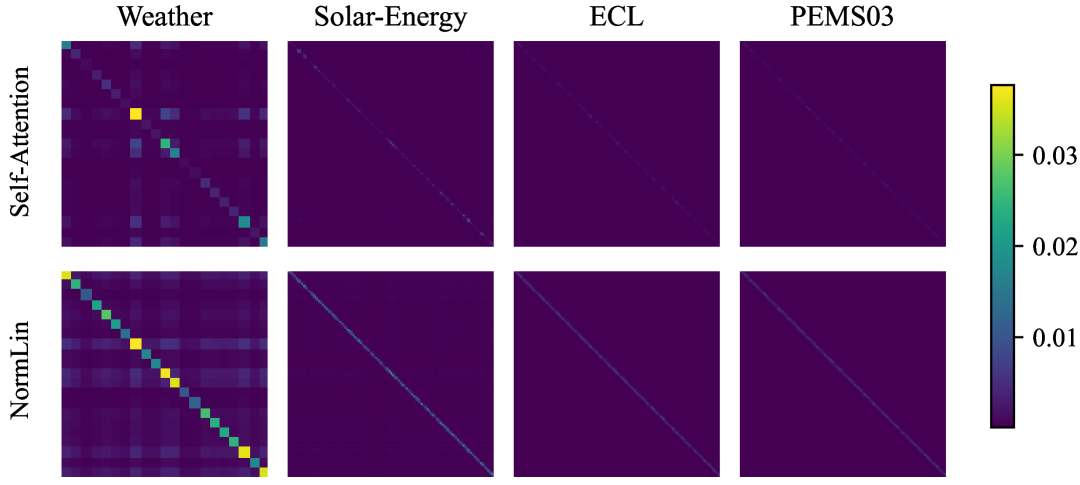
Figure 6: Comparison of Jacobian matrices of $\mathrm{Softmax}\left(\cdot\right)$ in self-attention and $\mathrm{Norm}_{\mathrm{L1}}\left(\mathrm{Softplus}\left(\cdot\right)\right)$ in the NormLin layer. The absolute values of the matrix entries are visualized. NormLin and self-attention exhibit similar patterns; however, NormLin generally yields diagonal entries of higher magnitude, suggesting more effective gradient propagation. The same input vector is used for both to ensure a fair comparison.

Appendix C Dataset description

Table 11: Detailed dataset descriptions and statistics. Dim denotes the number of variates for each dataset. Frequency refers to the time interval between consecutive steps. Split indicates the (Train, Validation, Test) ratio. Prediction len. represents the prediction lengths. For long-term forecasting, the input length is fixed at 96. For short-term forecasting, we adopt two settings: S1 (Input-12, Predict-$\{3,6,9,12\}$) and S2 (Input-36, Predict-$\{24,36,48,60\}$). In total, 140 prediction tasks across various datasets and prediction length settings are evaluated in this work.

Dataset	Dim	Frequency	Total len.	Split	Prediction len.	Information
ETTh1, ETTh2	7	Hourly	17420	6:2:2	{96,192,336,720}	Electricity
ETTm1, ETTm2	7	15 mins	69680	6:2:2	{96,192,336,720}	Electricity
Weather	21	10 mins	52696	7:1:2	{96,192,336,720}	Weather
ECL	321	Hourly	26304	7:1:2	{96,192,336,720}	Electricity
Traffic	862	Hourly	17544	7:1:2	{96,192,336,720}	Transportation
Exchange	8	Daily	7588	7:1:2	{96,192,336,720}	Economy
Solar-Energy	137	10 mins	52560	7:1:2	{96,192,336,720}	Energy
PEMS03	358	5 mins	26209	6:2:2	{12,24,48,96}	Transportation
PEMS04	307	5 mins	16992	6:2:2	{12,24,48,96}	Transportation
PEMS07	883	5 mins	28224	6:2:2	{12,24,48,96}	Transportation
PEMS08	170	5 mins	17856	6:2:2	{12,24,48,96}	Transportation
ILI	7	Weekly	966	7:1:2	{3,6,9,12} {24,36,48,60}	Health
COVID-19	55	Daily	335	7:1:2	{3,6,9,12}	Health
				6:2:2	{24,36,48,60}
METR-LA	207	5 mins	34272	7:1:2	{3,6,9,12} {24,36,48,60}	Transportation
NASDAQ	12	Daily	3914	7:1:2	{3,6,9,12} {24,36,48,60}	Finance
Wiki	99	Daily	730	7:1:2	{3,6,9,12} {24,36,48,60}	Web
SP500	5	Daily	8077	7:1:2	{3,6,9,12} {24,36,48,60}	Finance
DowJones	27	Daily	6577	7:1:2	{3,6,9,12} {24,36,48,60}	Finance
CarSales	10	Daily	6728	7:1:2	{3,6,9,12} {24,36,48,60}	Market
Power	2	Daily	1186	7:1:2	{3,6,9,12} {24,36,48,60}	Energy
Website	4	Daily	2167	7:1:2	{3,6,9,12} {24,36,48,60}	Web
Unemp	53	Monthly	531	6:2:2	{3,6,9,12} {24,36,48,60}	Society

In this work, the following real-world datasets are used for performance evaluation. The dataset details are presented in Table 11.

• ETT datasets [Zhou et al., 2021] record seven channels related to electricity transformers from July 2016 to July 2018. It contains four datasets: ETTh1 and ETTh2, with hourly recordings, and ETTm1 and ETTm2, with 15-minute recordings.

• Weather [Wu et al., 2021] contains 21 meteorological variables (e.g., air temperature, humidity) recorded every 10 minutes in 2020.

• ECL [Wu et al., 2021] records hourly electricity consumption of 321 consumers from July 2016 to July 2019.

• Traffic [Wu et al., 2021] includes hourly road occupancy rates from 862 sensors in the Bay Area from January 2015 to December 2016.

• Exchange [Wu et al., 2021] collects daily exchange rates for eight countries from January 1990 to October 2010.

• Solar-Energy [Lai et al., 2018] records the solar power output every 10 minutes from 137 photovoltaic plants in 2006.

• PEMS [Liu et al., 2022] provides public traffic sensor data from California, collected every 5 minutes. We use its four subsets (PEMS03, PEMS04, PEMS07, PEMS08) in this study.

• ILI contains weekly records of influenza-like illness patient counts provided by the U.S. CDC from 2002 to 2021.

• COVID-19 [Chen et al., 2022] includes daily records of COVID-19 hospitalizations in California in 2020, provided by Johns Hopkins University.

• METR-LA collects traffic network data in Los Angeles every 5 minutes from March to June 2012. A total of 207 channels are included.

• NASDAQ includes daily NASDAQ index and key economic indicators (e.g., interest rate and gold price) from 2010 to 2024.

• Wiki records daily page view counts for Wikipedia articles over two years (2018–2019). The first 99 channels are used in this study.

• SP500 records daily SP500 index data (e.g., opening price, closing price, and trading volume) from January 1993 to February 2025.

• DowJones collects daily stock prices of 27 Dow Jones Industrial Average (DJIA) component companies from January 1999 to March 2025.

• CarSales collects daily sales of 10 vehicle brands (e.g., Toyota, Honda) in the U.S. from January 2005 to June 2023. The data are compiled from the Vehicles Sales dataset on Kaggle.

• Power contains daily wind and solar energy production (in MW) records for the French grid from April 2020 to June 2023. The data are compiled from the Wind & Solar Daily Power Production dataset on Kaggle.

• Website contains six years of daily visit data (e.g., first-time and returning visits) to an academic website, spanning from September 2014 to August 2020.

• Unemp contains monthly unemployment figures for 50 U.S. states and three other territories from January 1976 to March 2020, sourced from the official website of the U.S. Bureau of Labor Statistics.

Appendix D Implementation details

OLinear is optimized using the ADAM optimizer [Kingma and Ba, 2015], with the initial learning rate selected from $\left\{10^{-4},2\times 10^{-4},5\times 10^{-4}\right\}$. The model dimension $D$ is chosen from $\left\{128,256,512\right\}$, while the embedding size $d$ is set to 16. The batch size is selected from $\left\{4,8,16,32\right\}$ depending on the dataset scale. The block number $L$ is chosen from $\left\{1,2,3\right\}$. Training is performed for up to 50 epochs with early stopping, which halts training if the validation performance does not improve for 10 consecutive epochs. We adopt the weighted L1 loss function following CARD [Wang et al., 2024b]. The experiments are implemented in PyTorch [Paszke et al., 2019] and conducted on an NVIDIA GPU with 24 GB of memory. Hyperparameter sensitivity is discussed in Appendix I.6. For baseline models, we use the reported values from the original papers when available; otherwise, we produce the results using the official code. For the model FilterNet [Yi et al., 2024a], TexFilter is adopted in this work. The code and datasets are available at the following anonymous repository: https://anonymous.4open.science/r/OLinear.

Appendix E Showcases

E.1 Time domain and transformed domain

Figure 5 illustrates the temporal domain and its corresponding transformed domain. In the transformed domain, the correlations along the sequence are effectively suppressed. Adjacent time series exhibit strong consistency in this new domain, which is desirable for forecasting tasks. The orthogonal transformation corresponds to projecting the time series onto the eigenvectors of the temporal Pearson correlation matrix $\mathrm{CorrMat}_{t}$. The eigenvalues of this symmetric positive semi-definite matrix $\mathrm{CorrMat}_{t}$ typically decay rapidly [Jolliffe, 2002], with only a few being dominant. Consequently, the transformed series exhibits sparsity, with most of the energy concentrated in just a few dimensions. Moreover, since noise tends to be evenly distributed across the transformed dimensions, the signal-to-noise ratio (SNR) in the leading components is improved [Bishop and Nasrabadi, 2006].

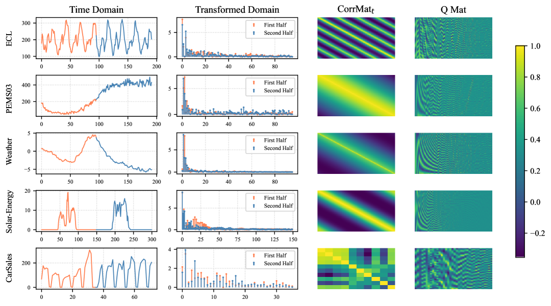
Figure 7: Visualization of temporal series, transformed series, the temporal Pearson correlation matrix, and its corresponding orthogonal matrix. The series are normalized prior to transformation, and the absolute values in the transformed domain are shown for clarity. The X-axis in the first and second columns represents the temporal and feature dimensions, respectively. Adjacent series exhibit consistency in the transformed domain, with sparsity clearly observable. Temporal Pearson correlation matrices on more datasets are presented in Figure 8.

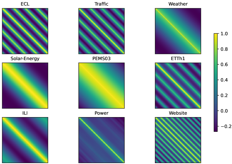
Figure 8: Temporal Pearson correlation matrices on various datasets. Periodic patterns are clearly reflected in the correlation matrices. We incorporate such a priori statistical information into the model design, leading to improved forecasting performance.

E.2 Low-rank attention matrix and high-rank NormLin weight matrix

We replace the NormLin module in OLinear with a standard self-attention mechanism and observe the typical low-rank property in the resulting attention matrices, as shown in Figure 9. This phenomenon can be attributed to the sparsity induced by the transformed domain and the sharp focus introduced by the Softmax operation. The low-rank attention matrix could limit the expressive capacity of the model. In contrast, the weight matrices in NormLin exhibit higher rank, better preserving representation diversity.

Furthermore, the learned NormLin weights closely resemble the across-variate Pearson correlation matrix $\mathrm{CorrMat}_{v}$, suggesting that the NormLin layer effectively captures multivariate correlations. By directly replacing the learnable weight matrix with $\mathrm{Softmax}(\mathrm{CorrMat}_{v})$, we obtain OLinear-C, which also achieves competitive performance, as demonstrated in Appendix H.

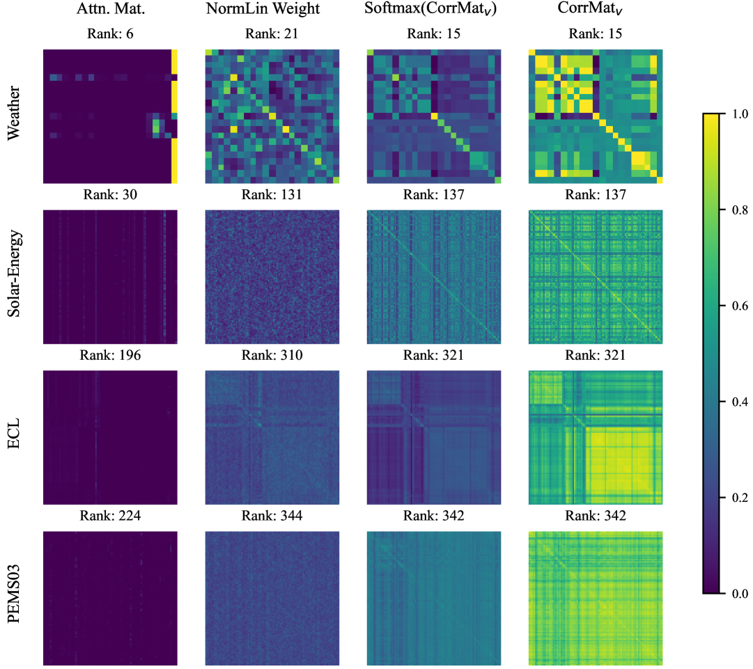
Figure 9: Illustration of attention/weight matrices from self-attention, NormLin, and the across-variate Pearson correlation matrices (with and without Softmax). When applied in OLinear, the self-attention mechanism results in low-rank attention matrices, whereas NormLin produces high-rank weight matrices that better preserve representation diversity. Moreover, the learned NormLin weights resemble the across-variate correlation matrices, suggesting effective modeling of multivariate relationships.

E.3 OrthoTrans enhances attention matrix rank

Figures 10–12 visualize the attention matrices of OLinear (with the NormLin module replaced by self-attention) under different transformation bases. Similar results for iTransformer and PatchTST are presented in Figures 13 and 14, respectively. As shown, OrthoTrans typically yields higher-rank attention matrices compared to DFT, wavelet transforms, or no transformation. As stated earlier, higher-rank attention matrices better preserve the representation space and can potentially enhance the model’s expressive capacity [Han et al., 2023]. This may explain why integrating OrthoTrans as a plug-in consistently improves the performance of Transformer-based forecasters (as shown in Table 5).

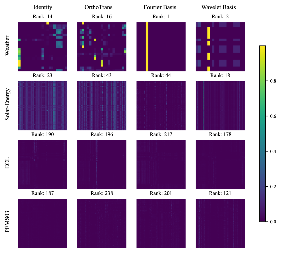
Figure 10: Comparison of attention matrices under various transformation bases for OLinear with the NormLin module replaced by self-attention (Example 1). For a fair comparison, the same input series is used for different bases on each dataset. ‘Identity’ denotes no transformation, and the Haar wavelet is used as the wavelet basis. In general, OrthoTrans yields higher-rank attention matrices and thus better preserves the representation space.

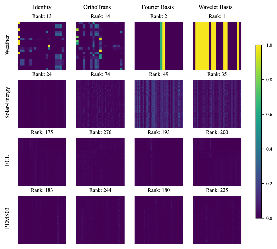
Figure 11: Comparison of attention matrices under various transformation bases for OLinear with the NormLin module replaced by self-attention (Example 2). For a fair comparison, the same input series is used across bases on each dataset. ‘Identity’ denotes no transformation, and the Haar wavelet is used as the wavelet basis. In general, OrthoTrans yields higher-rank attention matrices and thus better preserves the representation space.

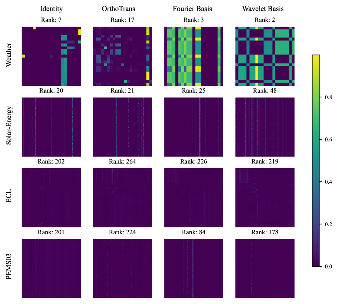
Figure 12: Comparison of attention matrices under various transformation bases for OLinear with the NormLin module replaced by self-attention (Example 3). For a fair comparison, the same input series is used across bases on each dataset. ‘Identity’ denotes no transformation, and the Haar wavelet is used as the wavelet basis. In general, OrthoTrans yields higher-rank attention matrices and thus better preserves the representation space.

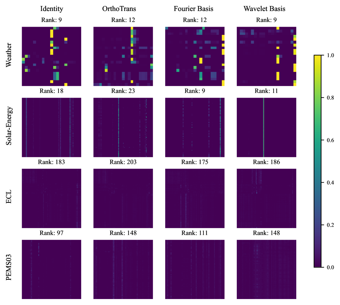
Figure 13: Comparison of attention matrices under various transformation bases for iTransformer. For a fair comparison, the same input series is used across bases on each dataset. ‘Identity’ denotes no transformation, and the Haar wavelet is used as the wavelet basis. In general, OrthoTrans yields higher-rank attention matrices and thus better preserves the representation space.

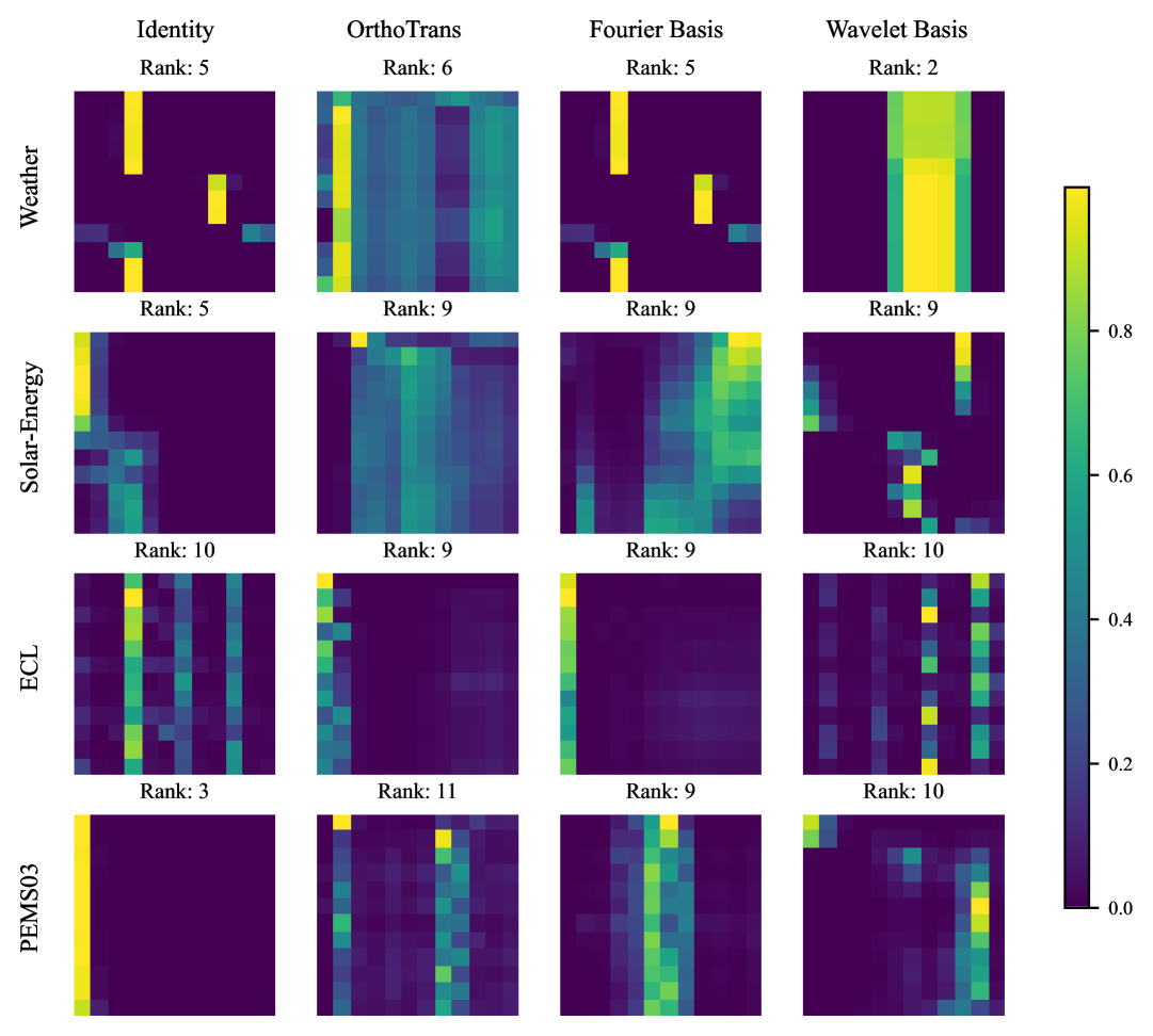
Figure 14: Comparison of attention matrices under various transformation bases for PatchTST. For a fair comparison, the same input series is used across all bases for each dataset. ‘Identity’ denotes no transformation, and the Haar wavelet is used as the wavelet basis. In general, OrthoTrans yields higher-rank attention matrices and thus better preserves the representation space.

Appendix F Robustness under various random seeds

Table 12 presents the standard deviations for different datasets and prediction lengths using seven random seeds. OLinear demonstrates strong robustness across independent runs. Furthermore, as shown in Table 13, our model exhibits better robustness than state-of-the-art Transformer-based models, TimeMixer++ and iTransformer, as measured by the 99% confidence intervals.

Note that averaging over $\mathcal{M}$ prediction lengths reduces the standard deviation by a factor of $\frac{1}{\sqrt{\mathcal{M}}}$, making the results more robust to the choice of random seeds. Therefore, we prefer to report the average results in this work to mitigate the influence of randomness.

Table 12: Robustness of OLinear performance. Standard deviations are calculated over seven random seeds. S1 and S2 correspond to $\mathrm{Input}-12,\mathrm{Predict}-\left\{3,6,9,12\right\}$ and $\mathrm{Input}-36,\mathrm{Predict}-\left\{24,36,48,60\right\}$, respectively.

Dataset		ECL		Traffic		ETTm1		Solar-Energy
Metric		MSE	MAE	MSE	MAE	MSE	MAE	MSE	MAE
Horizon	96	0.131±4e-4	0.221±4e-4	0.398±3e-3	0.226±2e-4	0.302±7e-4	0.334±3e-4	0.179±6e-4	0.191±5e-4
	192	0.150±1e-3	0.238±1e-3	0.439±3e-3	0.241±4e-4	0.357±9e-4	0.363±5e-4	0.209±8e-4	0.213±2e-4
	336	0.165±1e-3	0.254±1e-3	0.464±4e-3	0.250±3e-4	0.387±2e-3	0.385±5e-4	0.231±8e-4	0.229±7e-5
	720	0.191±2e-3	0.279±2e-3	0.502±4e-3	0.270±4e-4	0.452±1e-3	0.426±6e-4	0.241±1e-3	0.236±4e-4
Dataset		Weather		PEMS03		NASDAQ (S2)		Wiki (S1)
Metric		MSE	MAE	MSE	MAE	MSE	MAE	MSE	MAE
Horizon	H1	0.153±1e-3	0.190±1e-3	0.060±3e-4	0.159±3e-4	0.121±1e-3	0.216±9e-4	6.161±1e-2	0.368±7e-4
	H2	0.200±2e-3	0.235±2e-3	0.078±6e-4	0.179±5e-4	0.163±7e-4	0.261±9e-4	6.453±9e-3	0.385±1e-3
	H3	0.258±3e-3	0.280±2e-3	0.104±6e-4	0.210±6e-4	0.205±2e-3	0.296±2e-3	6.666±6e-3	0.398±1e-3
	H4	0.337±4e-3	0.333±2e-3	0.140±2e-3	0.247±1e-3	0.259±2e-3	0.336±2e-3	6.834±4e-3	0.406±4e-4
Dataset		DowJones (S2)		SP500 (S2)		CarSales (S1)		Power (S1)
Metric		MSE	MAE	MSE	MAE	MSE	MAE	MSE	MAE
Horizon	H1	7.432±3e-2	0.664±9e-4	0.155±2e-3	0.271±2e-3	0.303±2e-3	0.277±1e-3	0.864±7e-3	0.688±4e-3
	H2	10.848±7e-2	0.799±1e-3	0.209±2e-3	0.317±2e-3	0.315±2e-3	0.285±2e-3	0.991±7e-3	0.742±3e-3
	H3	14.045±1e-1	0.914±1e-3	0.258±2e-3	0.358±1e-3	0.327±8e-4	0.293±8e-4	1.062±1e-2	0.770±4e-3
	H4	16.959±8e-2	1.017±3e-3	0.305±3e-3	0.387±2e-3	0.336±5e-4	0.301±4e-4	1.119±2e-2	0.789±6e-3

Table 13: 99% confidence intervals of the average performance across four prediction lengths, computed using three times the standard deviation from seven random seeds. The smallest standard deviations are highlighted in bold. OLinear-C denotes the variant of OLinear where the weight matrix in NormLin is set to $\mathrm{Softmax}\left(\mathrm{CorrMat}_{v}\right)$, with $\mathrm{CorrMat}_{v}$ being the multivariate correlation matrix.

Model	OLinear (Ours)		OLinear-C (Ours)		TimeMixer++ 2025a		iTransformer 2024a
Metric	MSE	MAE	MSE	MAE	MSE	MAE	MSE	MAE
Weather	0.237±0.006	0.260± 0.003	0.238± 0.005	0.259±0.004	0.226±0.008	0.262±0.007	0.258±0.009	0.278±0.006
Solar	0.215± 0.001	0.217±0.001	0.215± 0.001	0.217± 3e-4	0.203± 0.001	0.238±0.010	0.233±0.009	0.262±0.007
ECL	0.159± 0.001	0.248±0.002	0.161±0.006	0.249±0.005	0.165±0.011	0.253± 0.001	0.178±0.002	0.270±0.005
Traffic	0.451± 0.003	0.247± 0.001	0.451±0.006	0.247± 0.001	0.416±0.015	0.264±0.013	0.428±0.008	0.282±0.002
ETTh1	0.424±0.003	0.424±0.002	0.424± 0.002	0.424± 0.001	0.419±0.011	0.432±0.015	0.454±0.004	0.447±0.007
ETTh2	0.367± 0.002	0.388±0.002	0.368± 0.002	0.389± 0.001	0.339±0.009	0.380±0.002	0.383±0.004	0.407±0.007
ETTm1	0.374± 0.001	0.377± 0.001	0.375± 0.001	0.378± 0.001	0.369±0.005	0.378±0.007	0.407±0.004	0.410±0.009
ETTm2	0.270± 3e-4	0.313± 2e-4	0.270±4e-4	0.313± 2e-4	0.269±0.002	0.320±0.012	0.288±0.010	0.332±0.003

Appendix G Full results

Table 14 lists the simplified tables from the main text and their full versions in the appendix.

Table 14: Overview of tables in the main paper and their full versions in the appendix.

Tables in paper	Tables in Appendix	Content
Table 2	Table 15	Long-term forecasting
Table  3	Tables 16 and 17	Short-term forecasting
Table 4	Table 18	Ablation studies on various bases
Table 5	Table 19	OrthoTrans as a plug-in
Table 7	Table 23	Performance of OLinear-C
Table 6	Table 20	Ablation studies of OLinear
Table 9	Table 21	NormLin vs self-attention and its variants
Table 9	Table 22	NormLin as a plug-in

Table 15: Full results for the long-term forecasting task. The lookback length $T$ is set to 96 for all baselines. Avg means the average results across four prediction lengths. This table presents the full version of Table 2.

Category		Linear-Based										Transformer-Based												TCN-Based
Model		OLinear (Ours)		TimeMixer 2024a		FilterNet 2024a		FITS 2024		DLinear 2023		TimeMixer++ 2025a		Leddam 2024		CARD 2024b		Fredformer 2024		iTrans. 2024a		PatchTST 2023		TimesNet 2023b
Metric		MSE	MAE	MSE	MAE	MSE	MAE	MSE	MAE	MSE	MAE	MSE	MAE	MSE	MAE	MSE	MAE	MSE	MAE	MSE	MAE	MSE	MAE	MSE	MAE
ETTm1	96	0.302	0.334	0.320	0.357	0.321	0.361	0.353	0.375	0.345	0.372	0.310	0.334	0.319	0.359	0.316	0.347	0.326	0.361	0.334	0.368	0.329	0.367	0.338	0.375
	192	0.357	0.363	0.361	0.381	0.367	0.387	0.486	0.445	0.380	0.389	0.348	0.362	0.369	0.383	0.363	0.370	0.363	0.380	0.377	0.391	0.367	0.385	0.374	0.387
	336	0.387	0.385	0.390	0.404	0.401	0.409	0.531	0.475	0.413	0.413	0.376	0.391	0.394	0.402	0.392	0.390	0.395	0.403	0.426	0.420	0.399	0.410	0.410	0.411
	720	0.452	0.426	0.454	0.441	0.477	0.448	0.600	0.513	0.474	0.453	0.440	0.423	0.460	0.442	0.458	0.425	0.453	0.438	0.491	0.459	0.454	0.439	0.478	0.450
	Avg	0.374	0.377	0.381	0.395	0.392	0.401	0.493	0.452	0.403	0.407	0.369	0.378	0.386	0.397	0.383	0.384	0.384	0.395	0.407	0.410	0.387	0.400	0.400	0.406
ETTm2	96	0.169	0.249	0.175	0.258	0.175	0.258	0.182	0.266	0.193	0.292	0.170	0.245	0.176	0.257	0.169	0.248	0.177	0.259	0.180	0.264	0.175	0.259	0.187	0.267
	192	0.232	0.290	0.237	0.299	0.240	0.301	0.253	0.312	0.284	0.362	0.229	0.291	0.243	0.303	0.234	0.292	0.243	0.301	0.250	0.309	0.241	0.302	0.249	0.309
	336	0.291	0.328	0.298	0.340	0.311	0.347	0.313	0.349	0.369	0.427	0.303	0.343	0.303	0.341	0.294	0.339	0.302	0.340	0.311	0.348	0.305	0.343	0.321	0.351
	720	0.389	0.387	0.391	0.396	0.414	0.405	0.416	0.406	0.554	0.522	0.373	0.399	0.400	0.398	0.390	0.388	0.397	0.396	0.412	0.407	0.402	0.400	0.408	0.403
	Avg	0.270	0.313	0.275	0.323	0.285	0.328	0.291	0.333	0.350	0.401	0.269	0.320	0.281	0.325	0.272	0.317	0.279	0.324	0.288	0.332	0.281	0.326	0.291	0.333
ETTh1	96	0.360	0.382	0.375	0.400	0.382	0.402	0.385	0.394	0.386	0.400	0.361	0.403	0.377	0.394	0.383	0.391	0.373	0.392	0.386	0.405	0.414	0.419	0.384	0.402
	192	0.416	0.414	0.429	0.421	0.430	0.429	0.434	0.422	0.437	0.432	0.416	0.441	0.424	0.422	0.435	0.420	0.433	0.420	0.441	0.436	0.460	0.445	0.436	0.429
	336	0.457	0.438	0.484	0.458	0.472	0.451	0.476	0.444	0.481	0.459	0.430	0.434	0.459	0.442	0.479	0.442	0.470	0.437	0.487	0.458	0.501	0.466	0.491	0.469
	720	0.463	0.462	0.498	0.482	0.481	0.473	0.465	0.462	0.519	0.516	0.467	0.451	0.463	0.459	0.471	0.461	0.467	0.456	0.503	0.491	0.500	0.488	0.521	0.500
	Avg	0.424	0.424	0.447	0.440	0.441	0.439	0.440	0.431	0.456	0.452	0.419	0.432	0.431	0.429	0.442	0.429	0.435	0.426	0.454	0.447	0.469	0.454	0.458	0.450
ETTh2	96	0.284	0.329	0.289	0.341	0.293	0.343	0.292	0.340	0.333	0.387	0.276	0.328	0.292	0.343	0.281	0.330	0.293	0.342	0.297	0.349	0.292	0.342	0.340	0.374
	192	0.360	0.379	0.372	0.392	0.374	0.396	0.377	0.391	0.477	0.476	0.342	0.379	0.367	0.389	0.363	0.381	0.371	0.389	0.380	0.400	0.387	0.400	0.402	0.414
	336	0.409	0.415	0.386	0.414	0.417	0.430	0.416	0.425	0.594	0.541	0.346	0.398	0.412	0.424	0.411	0.418	0.382	0.409	0.428	0.432	0.426	0.433	0.452	0.452
	720	0.415	0.431	0.412	0.434	0.449	0.460	0.418	0.437	0.831	0.657	0.392	0.415	0.419	0.438	0.416	0.431	0.415	0.434	0.427	0.445	0.431	0.446	0.462	0.468
	Avg	0.367	0.388	0.365	0.395	0.383	0.407	0.376	0.398	0.559	0.515	0.339	0.380	0.373	0.399	0.368	0.390	0.365	0.393	0.383	0.407	0.384	0.405	0.414	0.427
ECL	96	0.131	0.221	0.153	0.247	0.147	0.245	0.198	0.274	0.197	0.282	0.135	0.222	0.141	0.235	0.141	0.233	0.147	0.241	0.148	0.240	0.161	0.250	0.168	0.272
	192	0.150	0.238	0.166	0.256	0.160	0.250	0.363	0.422	0.196	0.285	0.147	0.235	0.159	0.252	0.160	0.250	0.165	0.258	0.162	0.253	0.199	0.289	0.184	0.289
	336	0.165	0.254	0.185	0.277	0.173	0.267	0.444	0.490	0.209	0.301	0.164	0.245	0.173	0.268	0.173	0.263	0.177	0.273	0.178	0.269	0.215	0.305	0.198	0.300
	720	0.191	0.279	0.225	0.310	0.210	0.309	0.532	0.551	0.245	0.333	0.212	0.310	0.201	0.295	0.197	0.284	0.213	0.304	0.225	0.317	0.256	0.337	0.220	0.320
	Avg	0.159	0.248	0.182	0.273	0.173	0.268	0.384	0.434	0.212	0.300	0.165	0.253	0.169	0.263	0.168	0.258	0.176	0.269	0.178	0.270	0.208	0.295	0.192	0.295
Exchange	96	0.082	0.200	0.086	0.205	0.091	0.211	0.087	0.208	0.088	0.218	0.085	0.214	0.086	0.207	0.084	0.202	0.084	0.202	0.086	0.206	0.088	0.205	0.107	0.234
	192	0.171	0.293	0.193	0.312	0.186	0.305	0.185	0.306	0.176	0.315	0.175	0.313	0.175	0.301	0.179	0.298	0.178	0.302	0.177	0.299	0.176	0.299	0.226	0.344
	336	0.331	0.414	0.356	0.433	0.380	0.449	0.342	0.425	0.313	0.427	0.316	0.420	0.325	0.415	0.333	0.418	0.319	0.408	0.331	0.417	0.301	0.397	0.367	0.448
	720	0.837	0.688	0.912	0.712	0.896	0.712	0.846	0.694	0.839	0.695	0.851	0.689	0.831	0.686	0.851	0.691	0.749	0.651	0.847	0.691	0.901	0.714	0.964	0.746
	Avg	0.355	0.399	0.387	0.416	0.388	0.419	0.365	0.408	0.354	0.414	0.357	0.409	0.354	0.402	0.362	0.402	0.333	0.391	0.360	0.403	0.367	0.404	0.416	0.443
Traffic	96	0.398	0.226	0.462	0.285	0.430	0.294	0.601	0.361	0.650	0.396	0.392	0.253	0.426	0.276	0.419	0.269	0.406	0.277	0.395	0.268	0.446	0.283	0.593	0.321
	192	0.439	0.241	0.473	0.296	0.452	0.307	0.603	0.365	0.598	0.370	0.402	0.258	0.458	0.289	0.443	0.276	0.426	0.290	0.417	0.276	0.540	0.354	0.617	0.336
	336	0.464	0.250	0.498	0.296	0.470	0.316	0.609	0.366	0.605	0.373	0.428	0.263	0.486	0.297	0.460	0.283	0.437	0.292	0.433	0.283	0.551	0.358	0.629	0.336
	720	0.502	0.270	0.506	0.313	0.498	0.323	0.648	0.387	0.645	0.394	0.441	0.282	0.498	0.313	0.490	0.299	0.462	0.305	0.467	0.302	0.586	0.375	0.640	0.350
	Avg	0.451	0.247	0.485	0.298	0.463	0.310	0.615	0.370	0.625	0.383	0.416	0.264	0.467	0.294	0.453	0.282	0.433	0.291	0.428	0.282	0.531	0.343	0.620	0.336
Weather	96	0.153	0.190	0.163	0.209	0.162	0.207	0.196	0.236	0.196	0.255	0.155	0.205	0.156	0.202	0.150	0.188	0.163	0.207	0.174	0.214	0.177	0.218	0.172	0.220
	192	0.200	0.235	0.208	0.250	0.210	0.250	0.240	0.271	0.237	0.296	0.201	0.245	0.207	0.250	0.202	0.238	0.211	0.251	0.221	0.254	0.225	0.259	0.219	0.261
	336	0.258	0.280	0.251	0.287	0.265	0.290	0.292	0.307	0.283	0.335	0.237	0.265	0.262	0.291	0.260	0.282	0.267	0.292	0.278	0.296	0.278	0.297	0.280	0.306
	720	0.337	0.333	0.339	0.341	0.342	0.340	0.365	0.354	0.345	0.381	0.312	0.334	0.343	0.343	0.343	0.353	0.343	0.341	0.358	0.349	0.354	0.348	0.365	0.359
	Avg	0.237	0.260	0.240	0.272	0.245	0.272	0.273	0.292	0.265	0.317	0.226	0.262	0.242	0.272	0.239	0.265	0.246	0.272	0.258	0.279	0.259	0.281	0.259	0.287
Solar-Energy	96	0.179	0.191	0.189	0.259	0.205	0.242	0.319	0.353	0.290	0.378	0.171	0.231	0.197	0.241	0.197	0.211	0.185	0.233	0.203	0.237	0.234	0.286	0.250	0.292
	192	0.209	0.213	0.222	0.283	0.233	0.265	0.367	0.387	0.320	0.398	0.218	0.263	0.231	0.264	0.234	0.234	0.227	0.253	0.233	0.261	0.267	0.310	0.296	0.318
	336	0.231	0.229	0.231	0.292	0.249	0.278	0.408	0.403	0.353	0.415	0.212	0.269	0.241	0.268	0.256	0.250	0.246	0.284	0.248	0.273	0.290	0.315	0.319	0.330
	720	0.241	0.236	0.223	0.285	0.253	0.281	0.411	0.395	0.356	0.413	0.212	0.270	0.250	0.281	0.260	0.254	0.247	0.276	0.249	0.275	0.289	0.317	0.338	0.337
	Avg	0.215	0.217	0.216	0.280	0.235	0.266	0.376	0.384	0.330	0.401	0.203	0.258	0.230	0.264	0.237	0.237	0.226	0.262	0.233	0.262	0.270	0.307	0.301	0.319
PEMS03	12	0.060	0.159	0.076	0.188	0.071	0.177	0.117	0.226	0.122	0.243	0.097	0.208	0.063	0.164	0.072	0.177	0.068	0.174	0.071	0.174	0.099	0.216	0.085	0.192
	24	0.078	0.179	0.113	0.226	0.102	0.213	0.235	0.324	0.201	0.317	0.120	0.230	0.080	0.185	0.107	0.217	0.093	0.202	0.093	0.201	0.142	0.259	0.118	0.223
	48	0.104	0.210	0.191	0.292	0.162	0.272	0.541	0.521	0.333	0.425	0.170	0.272	0.124	0.226	0.194	0.302	0.146	0.258	0.125	0.236	0.211	0.319	0.155	0.260
	96	0.140	0.247	0.288	0.363	0.244	0.340	1.062	0.790	0.457	0.515	0.274	0.342	0.160	0.266	0.323	0.402	0.228	0.330	0.164	0.275	0.269	0.370	0.228	0.317
	Avg	0.095	0.199	0.167	0.267	0.145	0.251	0.489	0.465	0.278	0.375	0.165	0.263	0.107	0.210	0.174	0.275	0.135	0.243	0.113	0.221	0.180	0.291	0.147	0.248
PEMS04	12	0.068	0.163	0.092	0.204	0.082	0.190	0.129	0.239	0.148	0.272	0.099	0.214	0.071	0.172	0.089	0.194	0.085	0.189	0.078	0.183	0.105	0.224	0.087	0.195
	24	0.079	0.176	0.128	0.243	0.110	0.224	0.246	0.337	0.224	0.340	0.115	0.231	0.087	0.193	0.128	0.234	0.117	0.224	0.095	0.205	0.153	0.275	0.103	0.215
	48	0.095	0.197	0.213	0.315	0.160	0.276	0.568	0.539	0.355	0.437	0.144	0.261	0.113	0.222	0.224	0.321	0.174	0.276	0.120	0.233	0.229	0.339	0.136	0.250
	96	0.122	0.226	0.307	0.384	0.234	0.343	1.181	0.843	0.452	0.504	0.185	0.297	0.141	0.252	0.382	0.445	0.273	0.354	0.150	0.262	0.291	0.389	0.190	0.303
	Avg	0.091	0.190	0.185	0.287	0.146	0.258	0.531	0.489	0.295	0.388	0.136	0.251	0.103	0.210	0.206	0.299	0.162	0.261	0.111	0.221	0.195	0.307	0.129	0.241
PEMS07	12	0.052	0.138	0.073	0.184	0.064	0.163	0.109	0.222	0.115	0.242	0.090	0.197	0.055	0.145	0.068	0.166	0.063	0.158	0.067	0.165	0.095	0.207	0.082	0.181
	24	0.065	0.151	0.111	0.219	0.093	0.200	0.230	0.327	0.210	0.329	0.110	0.219	0.070	0.164	0.103	0.206	0.089	0.192	0.088	0.190	0.150	0.262	0.101	0.204
	48	0.084	0.171	0.237	0.328	0.137	0.248	0.551	0.531	0.398	0.458	0.149	0.256	0.094	0.192	0.165	0.268	0.136	0.241	0.110	0.215	0.253	0.340	0.134	0.238
	96	0.108	0.196	0.303	0.354	0.198	0.306	1.112	0.809	0.594	0.553	0.258	0.359	0.117	0.217	0.258	0.346	0.197	0.298	0.139	0.245	0.346	0.404	0.181	0.279
	Avg	0.077	0.164	0.181	0.271	0.123	0.229	0.500	0.472	0.329	0.395	0.152	0.258	0.084	0.180	0.149	0.247	0.121	0.222	0.101	0.204	0.211	0.303	0.124	0.225
PEMS08	12	0.068	0.159	0.091	0.201	0.080	0.182	0.122	0.233	0.154	0.276	0.119	0.222	0.071	0.171	0.080	0.181	0.081	0.185	0.079	0.182	0.168	0.232	0.112	0.212
	24	0.089	0.178	0.137	0.246	0.114	0.219	0.236	0.330	0.248	0.353	0.149	0.249	0.091	0.189	0.118	0.220	0.112	0.214	0.115	0.219	0.224	0.281	0.141	0.238
	48	0.123	0.204	0.265	0.343	0.184	0.284	0.562	0.540	0.440	0.470	0.206	0.292	0.128	0.219	0.199	0.289	0.174	0.267	0.186	0.235	0.321	0.354	0.198	0.283
	96	0.173	0.236	0.410	0.407	0.309	0.356	1.216	0.846	0.674	0.565	0.329	0.355	0.198	0.266	0.405	0.431	0.277	0.335	0.221	0.267	0.408	0.417	0.320	0.351
	Avg	0.113	0.194	0.226	0.299	0.172	0.260	0.534	0.487	0.379	0.416	0.200	0.279	0.122	0.211	0.201	0.280	0.161	0.250	0.150	0.226	0.280	0.321	0.193	0.271
1st Count		33	49	0	0	0	0	0	0	0	0	29	14	1	0	2	1	2	2	0	0	1	1	0	0

Table 16: Full results for the short-term forecasting task (Part 1). For prediction lengths $\tau\in\left\{3,6,9,12\right\}$, the lookback horizon is $T=12$; for $\tau\in\left\{24,36,48,60\right\}$, it is $T=36$. The best results are highlighted in bold, and the second-best results are underlined. This table presents the detailed version of Table 3.

Model		OrthoLienar (Ours)		TimeMix. 2024a		FilterNet 2024a		FITS 2024		DLinear 2023		TimeMix.++ 2025a		Leddam 2024		CARD 2024b		Fredformer 2024		iTrans. 2024a		PatchTST 2023		TimesNet 2023b
Metric		MSE	MAE	MSE	MAE	MSE	MAE	MSE	MAE	MSE	MAE	MSE	MAE	MSE	MAE	MSE	MAE	MSE	MAE	MSE	MAE	MSE	MAE	MSE	MAE
ILI	3	0.468	0.349	0.659	0.435	0.660	0.437	1.461	0.743	1.280	0.747	0.658	0.430	0.551	0.388	0.597	0.392	0.528	0.403	0.555	0.395	0.646	0.417	0.627	0.420
	6	0.923	0.516	1.306	0.643	1.140	0.606	2.337	0.974	2.054	0.967	1.273	0.645	1.021	0.569	1.246	0.610	1.128	0.604	1.124	0.586	1.269	0.629	1.147	0.610
	9	1.289	0.655	2.070	0.842	1.815	0.798	3.397	1.197	2.771	1.138	2.009	0.840	1.881	0.795	2.041	0.829	1.804	0.786	1.794	0.772	2.021	0.830	1.796	0.785
	12	1.698	0.791	2.792	1.018	2.435	0.953	4.244	1.361	3.497	1.284	2.683	1.004	2.421	0.964	2.746	0.996	2.610	0.989	2.273	0.884	2.788	1.016	2.349	0.920
	Avg	1.094	0.578	1.707	0.734	1.512	0.698	2.860	1.069	2.400	1.034	1.656	0.730	1.468	0.679	1.658	0.707	1.518	0.696	1.437	0.659	1.681	0.723	1.480	0.684
	24	1.737	0.800	2.110	0.879	2.190	0.870	4.265	1.523	3.158	1.243	1.877	0.826	2.085	0.883	2.407	0.970	2.098	0.894	2.004	0.860	2.046	0.849	2.317	0.934
	36	1.714	0.795	2.084	0.890	1.902	0.862	3.718	1.363	3.009	1.200	2.276	0.912	2.017	0.892	2.324	0.948	1.712	0.867	1.910	0.880	2.344	0.912	1.972	0.920
	48	1.821	0.804	1.961	0.866	2.051	0.882	3.994	1.422	2.994	1.194	1.921	0.850	1.860	0.847	2.133	0.911	2.054	0.922	2.036	0.891	2.123	0.883	2.238	0.940
	60	1.785	0.810	1.926	0.878	2.151	0.925	4.543	1.554	3.172	1.232	1.745	0.838	1.967	0.879	2.177	0.921	1.925	0.913	2.022	0.919	2.001	0.895	2.027	0.928
	Avg	1.764	0.802	2.020	0.878	2.073	0.885	4.130	1.465	3.083	1.217	1.955	0.857	1.982	0.875	2.260	0.938	1.947	0.899	1.993	0.887	2.128	0.885	2.139	0.931
COVID-19	3	1.100	0.487	1.237	0.547	1.195	0.555	2.039	0.790	2.386	0.909	1.298	0.584	1.216	0.570	1.103	0.521	1.165	0.548	1.193	0.561	1.220	0.573	2.021	0.704
	6	1.750	0.619	2.003	0.739	1.839	0.711	2.683	0.919	3.220	1.053	1.833	0.682	1.782	0.689	1.919	0.735	1.465	0.685	1.933	0.755	1.982	0.762	2.405	0.808
	9	2.239	0.734	2.594	0.860	2.537	0.897	3.147	1.050	3.803	1.160	2.472	0.822	2.407	0.866	2.358	0.841	2.145	0.845	2.441	0.879	2.633	0.916	2.858	0.969
	12	2.538	0.831	3.103	0.981	2.782	0.956	3.630	1.156	4.524	1.288	3.273	1.084	2.851	0.991	2.857	0.971	2.833	0.984	2.819	0.984	3.050	1.030	2.993	0.964
	Avg	1.907	0.668	2.234	0.782	2.088	0.780	2.875	0.979	3.483	1.102	2.219	0.793	2.064	0.779	2.059	0.767	1.902	0.765	2.096	0.795	2.221	0.820	2.569	0.861
	24	4.474	1.180	6.335	1.554	5.926	1.517	8.248	1.829	9.780	1.851	6.539	1.618	4.860	1.342	5.133	1.394	4.799	1.347	4.715	1.321	5.528	1.450	5.634	1.442
	36	7.241	1.670	8.222	1.787	7.696	1.733	10.345	2.050	12.804	2.083	7.986	1.770	7.378	1.708	7.377	1.725	7.536	1.727	7.299	1.681	8.351	1.830	9.114	1.848
	48	10.076	1.985	11.669	2.157	11.572	2.141	11.999	2.197	14.244	2.189	11.655	2.156	10.051	1.999	11.013	2.103	9.833	1.951	10.141	2.012	11.259	2.114	10.940	2.033
	60	12.079	2.182	12.188	2.173	11.311	2.066	13.185	2.282	15.472	2.275	12.734	2.235	11.467	2.119	12.528	2.227	12.455	2.209	11.871	2.156	12.666	2.225	12.888	2.186
	Avg	8.467	1.754	9.604	1.918	9.126	1.864	10.944	2.089	13.075	2.099	9.728	1.945	8.439	1.792	9.013	1.862	8.656	1.808	8.506	1.792	9.451	1.905	9.644	1.877
METR-LA	3	0.207	0.171	0.205	0.192	0.204	0.189	0.211	0.198	0.218	0.231	0.204	0.189	0.204	0.191	0.210	0.180	0.205	0.188	0.205	0.188	0.204	0.190	0.221	0.204
	6	0.301	0.207	0.297	0.230	0.296	0.228	0.306	0.237	0.307	0.278	0.298	0.230	0.293	0.227	0.311	0.219	0.298	0.227	0.300	0.229	0.298	0.227	0.308	0.238
	9	0.382	0.238	0.381	0.264	0.377	0.261	0.392	0.271	0.386	0.316	0.384	0.266	0.369	0.264	0.401	0.253	0.385	0.263	0.386	0.265	0.382	0.263	0.387	0.273
	12	0.452	0.263	0.455	0.295	0.449	0.290	0.467	0.300	0.452	0.353	0.456	0.294	0.442	0.292	0.474	0.281	0.457	0.292	0.460	0.295	0.456	0.292	0.462	0.298
	Avg	0.335	0.220	0.334	0.245	0.331	0.242	0.344	0.251	0.341	0.294	0.335	0.245	0.327	0.243	0.349	0.233	0.336	0.242	0.338	0.244	0.335	0.243	0.344	0.253
	24	0.650	0.337	0.671	0.413	0.670	0.402	0.698	0.416	0.645	0.458	0.617	0.394	0.680	0.405	0.700	0.378	0.676	0.408	0.700	0.413	0.679	0.410	0.698	0.415
	36	0.800	0.388	0.841	0.480	0.824	0.471	0.874	0.490	0.785	0.533	0.781	0.457	0.841	0.471	0.874	0.448	0.852	0.477	0.867	0.480	0.845	0.484	0.856	0.475
	48	0.905	0.427	0.964	0.531	0.955	0.521	1.013	0.546	0.885	0.585	0.842	0.520	0.963	0.528	1.017	0.498	0.982	0.526	1.017	0.539	0.972	0.536	0.972	0.518
	60	0.999	0.457	1.047	0.573	1.050	0.563	1.122	0.589	0.959	0.623	0.958	0.551	1.029	0.556	1.126	0.541	1.084	0.569	1.079	0.572	1.077	0.578	1.033	0.543
	Avg	0.838	0.402	0.881	0.499	0.875	0.489	0.927	0.510	0.819	0.550	0.799	0.480	0.878	0.490	0.929	0.466	0.898	0.495	0.916	0.501	0.893	0.502	0.890	0.488
NASDAQ	3	0.036	0.092	0.035	0.093	0.038	0.100	0.042	0.111	0.044	0.123	0.036	0.098	0.040	0.103	0.037	0.096	0.039	0.102	0.040	0.105	0.038	0.099	0.049	0.123
	6	0.049	0.117	0.049	0.118	0.052	0.126	0.056	0.134	0.062	0.155	0.050	0.121	0.054	0.128	0.052	0.123	0.053	0.126	0.054	0.129	0.053	0.124	0.061	0.142
	9	0.062	0.137	0.062	0.139	0.065	0.145	0.069	0.154	0.082	0.189	0.063	0.144	0.066	0.147	0.063	0.141	0.067	0.147	0.068	0.150	0.065	0.145	0.073	0.161
	12	0.073	0.154	0.073	0.156	0.076	0.162	0.081	0.172	0.100	0.215	0.075	0.161	0.078	0.164	0.075	0.158	0.079	0.165	0.078	0.165	0.077	0.161	0.088	0.179
	Avg	0.055	0.125	0.055	0.126	0.058	0.133	0.062	0.142	0.072	0.170	0.056	0.131	0.059	0.135	0.057	0.130	0.059	0.135	0.060	0.137	0.058	0.132	0.068	0.151
	24	0.121	0.216	0.122	0.221	0.130	0.230	0.140	0.244	0.155	0.274	0.132	0.233	0.125	0.222	0.124	0.220	0.128	0.226	0.137	0.237	0.127	0.224	0.198	0.299
	36	0.163	0.261	0.183	0.279	0.175	0.273	0.184	0.284	0.196	0.306	0.177	0.278	0.174	0.271	0.167	0.266	0.170	0.268	0.184	0.280	0.174	0.269	0.229	0.326
	48	0.205	0.296	0.200	0.298	0.224	0.314	0.234	0.324	0.244	0.344	0.216	0.311	0.222	0.312	0.218	0.307	0.218	0.306	0.229	0.318	0.225	0.314	0.267	0.352
	60	0.259	0.336	0.238	0.328	0.259	0.340	0.282	0.357	0.318	0.401	0.249	0.337	0.264	0.341	0.264	0.341	0.262	0.339	0.279	0.352	0.265	0.339	0.327	0.394
	Avg	0.187	0.277	0.186	0.281	0.197	0.289	0.210	0.302	0.228	0.331	0.193	0.290	0.196	0.286	0.193	0.284	0.194	0.285	0.207	0.297	0.198	0.286	0.255	0.343
Wiki	3	6.161	0.368	6.209	0.392	6.234	0.402	7.470	0.496	6.254	0.438	6.149	0.389	6.148	0.383	6.183	0.378	6.190	0.387	6.237	0.393	6.112	0.380	7.597	0.510
	6	6.453	0.385	6.475	0.402	6.460	0.401	8.326	0.544	6.579	0.467	6.436	0.401	6.455	0.397	6.465	0.393	6.696	0.404	6.484	0.400	6.425	0.395	7.962	0.515
	9	6.666	0.398	6.702	0.418	6.697	0.416	8.869	0.564	6.776	0.508	6.714	0.420	6.687	0.412	6.714	0.415	6.768	0.411	6.689	0.411	6.743	0.426	8.150	0.524
	12	6.834	0.406	6.902	0.426	6.899	0.426	9.394	0.608	6.927	0.513	6.852	0.421	6.899	0.424	6.852	0.415	7.168	0.424	6.868	0.419	6.814	0.414	8.117	0.533
	Avg	6.528	0.389	6.572	0.409	6.572	0.411	8.515	0.553	6.634	0.481	6.538	0.408	6.547	0.404	6.553	0.400	6.705	0.406	6.569	0.405	6.523	0.404	7.956	0.520
	24	6.894	0.423	6.900	0.446	6.907	0.443	7.887	0.613	6.883	0.520	6.902	0.460	6.919	0.450	6.925	0.440	6.531	0.432	6.886	0.437	6.858	0.430	8.023	0.612
	36	6.446	0.439	6.520	0.467	6.514	0.467	7.774	0.660	6.393	0.538	6.539	0.473	6.456	0.457	6.463	0.451	5.935	0.453	6.431	0.452	6.400	0.445	7.229	0.595
	48	6.004	0.446	6.108	0.484	6.135	0.478	7.737	0.706	5.940	0.547	6.115	0.487	6.031	0.468	6.031	0.460	5.871	0.464	6.101	0.483	5.959	0.449	7.184	0.641
	60	5.705	0.454	5.732	0.476	5.811	0.482	7.855	0.746	5.605	0.552	5.736	0.497	5.740	0.478	5.723	0.463	5.389	0.463	5.681	0.462	5.633	0.452	6.805	0.645
	Avg	6.262	0.440	6.315	0.468	6.342	0.467	7.813	0.681	6.205	0.539	6.323	0.479	6.286	0.463	6.285	0.453	5.931	0.453	6.275	0.458	6.212	0.444	7.310	0.623
1st Count		19	47	8	1	2	1	0	0	0	0	7	0	6	0	0	0	10	1	0	0	5	1	0	0

Table 17: Full results for the short-term forecasting task (Part 2). For prediction lengths $\tau\in\left\{3,6,9,12\right\}$, the lookback horizon is $T=12$; for $\tau\in\left\{24,36,48,60\right\}$, it is $T=36$. The best and second-best results are highlighted in bold, and underlined, respectively. This table presents the detailed version of Table 3.

Model		OrthoLienar (Ours)		TimeMix. 2024a		FilterNet 2024a		FITS 2024		DLinear 2023		TimeMix.++ 2025a		Leddam 2024		CARD 2024b		Fredformer 2024		iTrans. 2024a		PatchTST 2023		TimesNet 2023b
Metric		MSE	MAE	MSE	MAE	MSE	MAE	MSE	MAE	MSE	MAE	MSE	MAE	MSE	MAE	MSE	MAE	MSE	MAE	MSE	MAE	MSE	MAE	MSE	MAE
SP500	3	0.035	0.126	0.038	0.137	0.046	0.154	0.046	0.157	0.047	0.152	0.040	0.141	0.047	0.155	0.036	0.130	0.045	0.153	0.046	0.155	0.042	0.146	0.037	0.133
	6	0.053	0.158	0.056	0.167	0.071	0.193	0.067	0.190	0.070	0.197	0.057	0.168	0.064	0.181	0.054	0.162	0.066	0.187	0.066	0.187	0.063	0.183	0.055	0.165
	9	0.070	0.181	0.074	0.192	0.080	0.203	0.087	0.218	0.091	0.220	0.076	0.196	0.081	0.206	0.072	0.184	0.080	0.205	0.080	0.203	0.081	0.207	0.071	0.187
	12	0.088	0.204	0.092	0.213	0.097	0.224	0.106	0.242	0.113	0.251	0.093	0.213	0.104	0.236	0.089	0.206	0.103	0.234	0.099	0.228	0.101	0.233	0.089	0.210
	Avg	0.061	0.167	0.065	0.177	0.073	0.193	0.076	0.202	0.080	0.205	0.066	0.179	0.074	0.194	0.063	0.170	0.073	0.195	0.073	0.193	0.072	0.192	0.063	0.174
	24	0.155	0.271	0.159	0.288	0.181	0.317	0.193	0.334	0.189	0.330	0.172	0.305	0.175	0.308	0.156	0.276	0.181	0.315	0.180	0.309	0.164	0.298	0.162	0.291
	36	0.209	0.317	0.218	0.343	0.224	0.341	0.259	0.389	0.250	0.363	0.227	0.344	0.232	0.358	0.206	0.319	0.239	0.365	0.225	0.346	0.221	0.341	0.219	0.344
	48	0.258	0.358	0.264	0.367	0.280	0.384	0.324	0.439	0.291	0.398	0.272	0.383	0.276	0.388	0.258	0.354	0.283	0.394	0.275	0.383	0.278	0.397	0.262	0.371
	60	0.305	0.387	0.322	0.416	0.332	0.416	0.391	0.486	0.377	0.475	0.319	0.413	0.325	0.423	0.303	0.385	0.341	0.438	0.322	0.418	0.321	0.409	0.305	0.399
	Avg	0.231	0.333	0.241	0.353	0.254	0.365	0.291	0.412	0.277	0.391	0.247	0.361	0.252	0.369	0.231	0.333	0.261	0.378	0.250	0.364	0.246	0.361	0.237	0.351
DowJones	3	1.550	0.276	1.568	0.276	1.587	0.278	1.611	0.283	1.574	0.280	1.555	0.278	1.538	0.277	1.563	0.276	1.563	0.277	1.551	0.276	1.556	0.276	2.269	0.325
	6	2.569	0.361	2.593	0.362	2.634	0.364	2.661	0.370	2.613	0.367	2.591	0.364	2.588	0.364	2.579	0.362	2.619	0.364	2.589	0.363	2.588	0.362	3.934	0.430
	9	3.565	0.430	3.564	0.431	3.651	0.434	3.704	0.443	3.621	0.436	3.572	0.433	3.644	0.440	3.569	0.430	3.575	0.432	3.599	0.433	3.585	0.432	4.715	0.492
	12	4.517	0.490	4.472	0.490	4.634	0.496	4.666	0.503	4.586	0.497	4.630	0.496	4.622	0.498	4.528	0.490	4.605	0.493	4.579	0.493	4.533	0.492	5.999	0.561
	Avg	3.050	0.389	3.049	0.390	3.126	0.393	3.160	0.400	3.099	0.395	3.087	0.393	3.098	0.395	3.060	0.389	3.090	0.391	3.079	0.391	3.065	0.390	4.229	0.452
	24	7.432	0.664	8.327	0.683	8.000	0.683	7.974	0.690	7.590	0.670	8.283	0.689	8.029	0.679	7.416	0.665	7.758	0.672	7.925	0.677	7.641	0.670	11.535	0.834
	36	10.848	0.799	11.192	0.813	12.011	0.823	11.907	0.837	10.986	0.803	14.754	0.856	11.962	0.828	10.799	0.798	11.456	0.808	12.087	0.827	11.210	0.807	16.922	0.982
	48	14.045	0.914	15.278	0.945	14.814	0.933	15.821	0.969	14.157	0.922	16.893	0.970	15.266	0.937	13.881	0.912	14.696	0.921	14.787	0.930	14.866	0.935	19.501	1.093
	60	16.959	1.017	20.997	1.067	18.932	1.054	19.320	1.077	18.018	1.035	18.881	1.059	18.407	1.045	17.257	1.021	18.058	1.032	18.298	1.041	17.947	1.036	22.804	1.177
	Avg	12.321	0.848	13.948	0.877	13.439	0.873	13.755	0.893	12.688	0.857	14.703	0.893	13.416	0.872	12.338	0.849	12.992	0.858	13.274	0.869	12.916	0.862	17.690	1.021
CarSales	3	0.303	0.277	0.307	0.296	0.304	0.291	0.411	0.375	0.396	0.383	0.309	0.289	0.316	0.300	0.318	0.295	0.311	0.300	0.281	0.276	0.300	0.290	0.315	0.303
	6	0.315	0.285	0.327	0.307	0.317	0.300	0.401	0.367	0.390	0.376	0.324	0.300	0.320	0.303	0.335	0.307	0.326	0.309	0.294	0.285	0.311	0.295	0.319	0.306
	9	0.327	0.293	0.336	0.315	0.329	0.308	0.418	0.380	0.406	0.390	0.331	0.306	0.332	0.311	0.351	0.319	0.339	0.318	0.305	0.292	0.324	0.306	0.338	0.318
	12	0.336	0.301	0.343	0.319	0.335	0.312	0.424	0.385	0.410	0.390	0.343	0.314	0.336	0.313	0.357	0.324	0.348	0.324	0.314	0.298	0.331	0.310	0.338	0.320
	Avg	0.320	0.289	0.328	0.309	0.321	0.303	0.413	0.377	0.400	0.385	0.327	0.302	0.326	0.306	0.340	0.311	0.331	0.313	0.298	0.288	0.316	0.300	0.327	0.312
	24	0.320	0.302	0.320	0.318	0.318	0.319	0.359	0.347	0.354	0.350	0.323	0.320	0.325	0.322	0.337	0.321	0.319	0.326	0.303	0.312	0.319	0.319	0.316	0.328
	36	0.334	0.315	0.332	0.331	0.331	0.330	0.373	0.360	0.368	0.365	0.351	0.348	0.337	0.333	0.348	0.333	0.333	0.335	0.318	0.323	0.332	0.330	0.338	0.343
	48	0.347	0.327	0.345	0.343	0.342	0.341	0.385	0.370	0.382	0.379	0.351	0.342	0.351	0.346	0.362	0.345	0.349	0.344	0.331	0.332	0.347	0.344	0.349	0.351
	60	0.358	0.337	0.355	0.351	0.352	0.349	0.399	0.385	0.388	0.380	0.363	0.352	0.361	0.353	0.372	0.353	0.359	0.349	0.344	0.342	0.355	0.348	0.359	0.359
	Avg	0.340	0.320	0.338	0.336	0.336	0.335	0.379	0.365	0.373	0.368	0.347	0.340	0.343	0.338	0.355	0.338	0.340	0.338	0.324	0.327	0.338	0.335	0.340	0.345
Power	3	0.864	0.688	0.850	0.683	0.842	0.685	0.899	0.712	0.876	0.708	0.843	0.685	0.859	0.696	0.896	0.691	0.865	0.697	0.863	0.696	0.830	0.687	0.929	0.716
	6	0.991	0.742	0.971	0.743	0.988	0.747	1.079	0.785	0.991	0.761	0.997	0.748	1.023	0.761	1.013	0.750	0.994	0.751	0.990	0.748	0.948	0.741	1.070	0.773
	9	1.062	0.770	1.024	0.763	1.063	0.778	1.150	0.804	1.051	0.790	1.050	0.767	1.071	0.783	1.085	0.781	1.073	0.784	1.065	0.780	1.027	0.773	1.104	0.788
	12	1.119	0.789	1.087	0.788	1.125	0.803	1.266	0.851	1.110	0.814	1.107	0.792	1.130	0.804	1.124	0.792	1.135	0.807	1.142	0.808	1.083	0.797	1.212	0.825
	Avg	1.009	0.747	0.983	0.744	1.004	0.753	1.098	0.788	1.007	0.768	0.999	0.748	1.021	0.761	1.029	0.753	1.017	0.760	1.015	0.758	0.972	0.749	1.079	0.775
	24	1.343	0.870	1.341	0.881	1.410	0.916	1.491	0.944	1.390	0.916	1.340	0.877	1.397	0.909	1.406	0.886	1.410	0.913	1.462	0.924	1.468	0.935	1.494	0.924
	36	1.445	0.903	1.420	0.914	1.590	0.968	1.621	0.994	1.518	0.957	1.446	0.920	1.509	0.951	1.506	0.921	1.538	0.953	1.582	0.964	1.593	0.972	1.526	0.950
	48	1.559	0.946	1.567	0.963	1.680	1.009	1.775	1.052	1.610	0.995	1.467	0.933	1.646	0.999	1.583	0.957	1.652	1.008	1.696	1.011	1.710	1.020	1.581	0.981
	60	1.602	0.971	1.609	0.988	1.776	1.053	1.958	1.122	1.679	1.020	1.626	1.006	1.727	1.043	1.693	1.003	1.752	1.049	1.796	1.061	1.829	1.064	1.625	1.010
	Avg	1.487	0.922	1.484	0.937	1.614	0.986	1.711	1.028	1.549	0.972	1.470	0.934	1.570	0.975	1.547	0.942	1.588	0.981	1.634	0.990	1.650	0.998	1.556	0.966
Website	3	0.077	0.199	0.086	0.215	0.084	0.213	0.191	0.320	0.159	0.288	0.083	0.208	0.082	0.210	0.099	0.225	0.080	0.207	0.072	0.198	0.089	0.217	0.075	0.200
	6	0.103	0.227	0.124	0.248	0.116	0.242	0.235	0.356	0.182	0.302	0.115	0.237	0.114	0.239	0.135	0.255	0.116	0.241	0.098	0.227	0.121	0.246	0.105	0.232
	9	0.135	0.251	0.159	0.275	0.151	0.269	0.276	0.372	0.220	0.330	0.156	0.273	0.147	0.266	0.171	0.282	0.150	0.268	0.124	0.252	0.157	0.273	0.138	0.262
	12	0.176	0.281	0.204	0.306	0.194	0.297	0.409	0.484	0.255	0.355	0.193	0.296	0.196	0.298	0.213	0.307	0.196	0.301	0.144	0.269	0.200	0.302	0.169	0.285
	Avg	0.123	0.240	0.143	0.261	0.136	0.255	0.278	0.383	0.204	0.319	0.137	0.253	0.135	0.253	0.154	0.267	0.135	0.254	0.109	0.237	0.141	0.259	0.122	0.244
	24	0.186	0.306	0.229	0.335	0.273	0.357	0.431	0.469	0.315	0.393	0.231	0.349	0.240	0.345	0.325	0.370	0.216	0.335	0.181	0.305	0.245	0.350	0.276	0.358
	36	0.272	0.356	0.361	0.420	0.401	0.441	0.554	0.552	0.385	0.447	0.328	0.397	0.327	0.405	0.428	0.442	0.331	0.411	0.226	0.342	0.370	0.429	0.377	0.436
	48	0.365	0.391	0.501	0.507	0.530	0.522	0.694	0.647	0.436	0.486	0.450	0.473	0.446	0.475	0.457	0.478	0.483	0.496	0.263	0.370	0.504	0.513	0.389	0.446
	60	0.486	0.481	0.571	0.562	0.630	0.592	0.736	0.673	0.468	0.510	0.525	0.517	0.561	0.549	0.596	0.566	0.556	0.547	0.323	0.410	0.587	0.565	0.478	0.507
	Avg	0.327	0.383	0.415	0.456	0.458	0.478	0.604	0.585	0.401	0.459	0.384	0.434	0.393	0.443	0.451	0.464	0.396	0.447	0.248	0.357	0.426	0.464	0.380	0.437
Unemp	3	0.012	0.047	0.015	0.074	0.012	0.062	0.161	0.289	0.072	0.200	0.014	0.069	0.013	0.061	0.014	0.070	0.013	0.068	0.012	0.061	0.012	0.060	0.062	0.171
	6	0.041	0.108	0.057	0.154	0.043	0.130	0.229	0.345	0.115	0.255	0.079	0.194	0.040	0.122	0.042	0.127	0.046	0.139	0.047	0.136	0.043	0.127	0.111	0.227
	9	0.084	0.170	0.109	0.213	0.107	0.216	0.369	0.443	0.191	0.329	0.101	0.200	0.119	0.226	0.093	0.194	0.095	0.198	0.098	0.199	0.093	0.190	0.176	0.281
	12	0.131	0.220	0.195	0.293	0.155	0.255	0.475	0.500	0.240	0.386	0.196	0.291	0.141	0.239	0.155	0.256	0.148	0.250	0.158	0.256	0.164	0.261	0.240	0.326
	Avg	0.067	0.136	0.094	0.183	0.079	0.166	0.308	0.394	0.154	0.292	0.097	0.188	0.078	0.162	0.076	0.162	0.075	0.163	0.079	0.163	0.078	0.160	0.147	0.251
	24	0.458	0.447	0.668	0.549	0.655	0.548	2.520	1.255	0.951	0.645	0.779	0.578	0.861	0.645	0.583	0.522	0.545	0.496	0.719	0.595	0.620	0.536	1.798	0.967
	36	0.870	0.619	1.580	0.866	1.247	0.769	4.478	1.703	0.906	0.717	1.318	0.777	1.741	0.938	1.205	0.762	1.107	0.725	2.212	1.103	2.245	1.120	2.820	1.171
	48	1.643	0.900	3.702	1.483	2.700	1.209	6.385	2.052	0.974	0.747	2.977	1.258	3.526	1.427	2.737	1.218	6.192	2.055	2.577	1.178	2.644	1.191	5.909	1.620
	60	2.593	1.182	6.320	2.030	5.370	1.830	8.460	2.392	1.071	0.798	6.582	2.060	5.574	1.857	4.475	1.624	8.236	2.384	5.441	1.799	4.074	1.511	7.511	2.053
	Avg	1.391	0.787	3.068	1.232	2.493	1.089	5.461	1.850	0.975	0.727	2.914	1.168	2.925	1.217	2.250	1.031	4.020	1.415	2.737	1.169	2.396	1.089	4.510	1.452
1st Count		18	35	5	6	1	0	0	0	3	3	3	1	2	0	7	9	0	0	21	14	5	2	0	0

Table 18: Comparison of different transformation bases. For S1 and S2, the prediction lengths are $\tau\in\{3,6,9,12\}$ and $\tau\in\{24,36,48,60\}$, respectively. Wavelet1 and Wavelet2 denote the classic Haar and discrete Meyer wavelets, respectively. Identity means that no transformation is applied. This is a complete version of Table 4.

Base		ECL		Solar-Energy		PEMS03		Power (S2)		ILI (S1)		COVID-19 (S2)		METR-LA (S2)
Metric		MSE	MAE	MSE	MAE	MSE	MAE	MSE	MAE	MSE	MAE	MSE	MAE	MSE	MAE
	H1	0.131	0.221	0.179	0.191	0.060	0.159	1.343	0.870	0.468	0.349	4.474	1.180	0.650	0.337
	H2	0.150	0.238	0.209	0.213	0.078	0.179	1.445	0.903	0.923	0.516	7.241	1.670	0.800	0.388
	H3	0.165	0.254	0.231	0.229	0.104	0.210	1.559	0.946	1.289	0.655	10.076	1.985	0.905	0.427
	H4	0.191	0.279	0.241	0.236	0.140	0.247	1.602	0.971	1.698	0.791	12.079	2.182	0.999	0.457
Ours	Avg	0.159	0.248	0.215	0.217	0.095	0.199	1.487	0.922	1.094	0.578	8.467	1.754	0.838	0.402
	H1	0.132	0.222	0.181	0.193	0.061	0.161	1.469	0.917	0.486	0.350	5.192	1.378	0.654	0.337
	H2	0.153	0.241	0.214	0.215	0.078	0.182	1.584	0.962	0.885	0.500	7.553	1.699	0.799	0.390
	H3	0.165	0.253	0.236	0.232	0.110	0.216	1.625	0.970	1.438	0.664	11.096	2.070	0.910	0.427
	H4	0.195	0.283	0.247	0.238	0.155	0.258	1.778	1.020	2.264	0.822	12.819	2.209	1.007	0.459
Fourier	Avg	0.161	0.250	0.219	0.219	0.101	0.204	1.614	0.967	1.268	0.584	9.165	1.839	0.843	0.403
	H1	0.134	0.223	0.182	0.194	0.061	0.161	1.476	0.917	0.483	0.351	4.826	1.317	0.647	0.336
	H2	0.153	0.241	0.217	0.216	0.079	0.183	1.586	0.959	0.943	0.520	7.117	1.652	0.801	0.390
	H3	0.166	0.255	0.238	0.234	0.114	0.219	1.711	1.011	1.251	0.653	10.133	1.995	0.903	0.428
	H4	0.186	0.276	0.250	0.240	0.176	0.278	1.880	1.060	1.786	0.795	12.588	2.233	1.011	0.464
Wavelet1	Avg	0.160	0.249	0.221	0.221	0.107	0.210	1.663	0.987	1.116	0.580	8.666	1.799	0.840	0.404
	H1	0.133	0.222	0.186	0.198	0.062	0.162	1.511	0.929	0.461	0.349	5.398	1.413	0.653	0.340
	H2	0.154	0.243	0.222	0.220	0.080	0.184	1.570	0.953	0.935	0.526	7.199	1.663	0.803	0.392
	H3	0.165	0.255	0.242	0.236	0.115	0.221	1.701	1.005	1.393	0.683	10.616	2.051	0.909	0.432
	H4	0.196	0.283	0.254	0.243	0.175	0.272	1.876	1.060	1.921	0.818	12.583	2.232	1.007	0.462
Wavelet2	Avg	0.162	0.251	0.226	0.224	0.108	0.210	1.664	0.987	1.177	0.594	8.949	1.840	0.843	0.406
	H1	0.134	0.223	0.184	0.198	0.061	0.160	1.338	0.864	0.456	0.341	5.381	1.391	0.661	0.339
	H2	0.156	0.244	0.220	0.222	0.079	0.182	1.564	0.969	0.945	0.524	8.001	1.767	0.803	0.391
	H3	0.182	0.270	0.244	0.240	0.118	0.220	1.604	0.950	1.527	0.700	11.244	2.108	0.923	0.433
	H4	0.399	0.444	0.256	0.246	0.163	0.266	1.774	1.076	1.940	0.824	12.695	2.233	1.028	0.466
Chebyshev	Avg	0.218	0.295	0.226	0.226	0.105	0.207	1.570	0.965	1.217	0.597	9.330	1.875	0.854	0.407
	H1	0.139	0.227	0.192	0.204	0.065	0.167	1.425	0.899	0.595	0.395	5.632	1.456	0.659	0.346
	H2	0.156	0.243	0.227	0.227	0.085	0.191	1.658	0.985	1.083	0.577	8.729	1.859	0.829	0.407
	H3	0.173	0.262	0.251	0.244	0.122	0.226	1.774	1.013	1.581	0.737	10.381	2.024	0.933	0.444
	H4	0.199	0.286	0.261	0.248	0.171	0.271	1.780	1.039	2.155	0.896	12.467	2.221	1.053	0.484
Laguerre	Avg	0.167	0.255	0.233	0.230	0.111	0.214	1.659	0.984	1.353	0.651	9.302	1.890	0.868	0.420
	H1	0.134	0.224	0.200	0.208	0.074	0.181	1.502	0.926	0.501	0.366	4.965	1.350	0.652	0.337
	H2	0.152	0.239	0.238	0.231	0.080	0.183	1.603	0.962	0.964	0.529	7.396	1.703	0.799	0.389
	H3	0.165	0.256	0.262	0.247	0.113	0.219	1.790	1.031	1.446	0.695	9.481	1.935	0.900	0.427
	H4	0.193	0.282	0.274	0.253	0.168	0.269	1.846	1.060	1.799	0.822	12.358	2.203	1.015	0.463
Legendre	Avg	0.161	0.250	0.243	0.235	0.109	0.213	1.685	0.995	1.177	0.603	8.550	1.798	0.841	0.404
	H1	0.134	0.224	0.186	0.199	0.063	0.163	1.419	0.900	0.477	0.352	4.841	1.284	0.659	0.342
	H2	0.156	0.245	0.221	0.220	0.080	0.184	1.453	0.903	0.956	0.523	7.828	1.757	0.807	0.395
	H3	0.167	0.257	0.244	0.237	0.117	0.222	1.582	0.956	1.307	0.659	10.153	2.003	0.921	0.433
	H4	0.194	0.282	0.256	0.244	0.165	0.266	1.715	1.023	1.874	0.812	12.603	2.232	1.006	0.461
Identity	Avg	0.163	0.252	0.227	0.225	0.106	0.209	1.542	0.945	1.153	0.587	8.856	1.819	0.848	0.408

Table 19: Full results of applying OrthoTrans to iTransformer, PatchTST and RLinear. ‘Imp.’ denotes the improvement over the corresponding vanilla model. Note that RLinear consists of only a single linear layer that projects the lookback length $T$ to the prediction horizon $\tau$. Nevertheless, OrthoTrans consistently improves RLinear’s performance, demonstrating its ability to enhance model capacity. This table is the complete version of Table 5.

		iTransformer 2024a				PatchTST 2023				RLinear 2023
Model		Vanilla		+OrthoTrans		Vanilla		+OrthoTrans		Vanilla		+OrthoTrans
Metric		MSE	MAE	MSE	MAE	MSE	MAE	MSE	MAE	MSE	MAE	MSE	MAE
	96	0.334	0.368	0.334	0.367	0.329	0.367	0.322	0.359	0.355	0.376	0.348	0.366
	192	0.377	0.391	0.377	0.389	0.367	0.385	0.363	0.383	0.391	0.392	0.386	0.385
	336	0.426	0.420	0.414	0.413	0.399	0.410	0.394	0.405	0.424	0.415	0.419	0.406
	720	0.491	0.459	0.490	0.452	0.454	0.439	0.457	0.445	0.487	0.450	0.478	0.439
	Avg	0.407	0.410	0.404	0.405	0.387	0.400	0.384	0.398	0.414	0.407	0.408	0.399
ETTm1	Imp.	–	–	0.80%	1.16%	–	–	0.82%	0.53%	–	–	1.51%	1.97%
	96	0.148	0.240	0.136	0.233	0.161	0.250	0.153	0.243	0.201	0.281	0.197	0.273
	192	0.162	0.253	0.155	0.250	0.199	0.289	0.165	0.254	0.201	0.283	0.196	0.276
	336	0.178	0.269	0.169	0.265	0.215	0.305	0.182	0.272	0.215	0.298	0.211	0.291
	720	0.225	0.317	0.225	0.311	0.256	0.337	0.222	0.306	0.257	0.331	0.253	0.324
	Avg	0.178	0.270	0.171	0.265	0.208	0.295	0.181	0.269	0.219	0.298	0.214	0.291
ECL	Imp.	–	–	3.97%	1.87%	–	–	13.12%	8.98%	–	–	2.17%	2.35%
	12	0.071	0.174	0.062	0.164	0.099	0.216	0.073	0.176	0.126	0.236	0.117	0.226
	24	0.093	0.201	0.080	0.185	0.142	0.259	0.104	0.210	0.246	0.334	0.233	0.322
	48	0.125	0.236	0.112	0.222	0.211	0.319	0.181	0.268	0.551	0.529	0.532	0.514
	96	0.164	0.275	0.160	0.269	0.269	0.370	0.293	0.338	1.057	0.787	1.024	0.760
	Avg	0.113	0.221	0.103	0.210	0.180	0.291	0.163	0.248	0.495	0.472	0.477	0.456
PEMS03	Imp.	–	–	8.45%	5.02%	–	–	9.69%	14.81%	–	–	3.74%	3.50%
	12	0.067	0.165	0.055	0.147	0.095	0.207	0.065	0.160	0.118	0.235	0.109	0.221
	24	0.088	0.190	0.071	0.165	0.150	0.262	0.097	0.192	0.242	0.341	0.228	0.324
	48	0.110	0.215	0.093	0.188	0.253	0.340	0.164	0.247	0.562	0.541	0.539	0.522
	96	0.139	0.245	0.122	0.218	0.346	0.404	0.264	0.311	1.096	0.795	1.065	0.773
	Avg	0.101	0.204	0.085	0.179	0.211	0.303	0.147	0.227	0.504	0.478	0.485	0.460
PEMS07	Imp.	–	–	15.59%	11.94%	–	–	30.17%	24.94%	–	–	3.76%	3.77%
	96	0.203	0.237	0.194	0.237	0.234	0.286	0.208	0.248	0.322	0.339	0.302	0.327
	192	0.233	0.261	0.231	0.265	0.267	0.310	0.237	0.268	0.359	0.356	0.342	0.346
	336	0.248	0.273	0.242	0.272	0.290	0.315	0.255	0.281	0.397	0.369	0.384	0.362
	720	0.249	0.275	0.245	0.275	0.289	0.317	0.255	0.281	0.397	0.356	0.387	0.356
	Avg	0.233	0.262	0.228	0.262	0.270	0.307	0.239	0.269	0.369	0.356	0.354	0.348
Solar-Energy	Imp.	–	–	2.16%	0.00%	–	–	11.57%	12.22%	–	–	4.14%	2.37%
	96	0.174	0.214	0.164	0.208	0.177	0.218	0.164	0.209	0.192	0.232	0.192	0.232
	192	0.221	0.254	0.221	0.259	0.225	0.259	0.211	0.251	0.240	0.271	0.236	0.268
	336	0.278	0.296	0.271	0.295	0.278	0.297	0.266	0.292	0.292	0.307	0.288	0.304
	720	0.358	0.349	0.351	0.347	0.354	0.348	0.345	0.343	0.364	0.353	0.359	0.350
	Avg	0.258	0.279	0.252	0.277	0.259	0.281	0.246	0.274	0.272	0.291	0.269	0.289
Weather	Imp.	–	–	2.42%	0.63%	–	–	4.86%	2.59%	–	–	1.22%	0.86%
	3	0.205	0.188	0.205	0.189	0.204	0.190	0.203	0.187	0.210	0.195	0.208	0.194
	6	0.300	0.229	0.292	0.227	0.298	0.227	0.296	0.228	0.304	0.234	0.303	0.235
	9	0.386	0.265	0.375	0.260	0.382	0.263	0.380	0.263	0.389	0.268	0.387	0.266
	12	0.460	0.295	0.444	0.291	0.456	0.292	0.452	0.294	0.465	0.298	0.464	0.297
	Avg	0.338	0.244	0.329	0.242	0.335	0.243	0.333	0.243	0.342	0.249	0.341	0.248
METR-LA	Imp.	–	–	2.55%	1.02%	–	–	0.67%	0.00%	–	–	0.44%	0.28%

Table 20: Ablation results for replacing or removing components along the variate and temporal dimensions. ‘Hor.’ denotes the prediction horizon. The simplified results are presented in Table 6.

			ECL		Traffic		Solar		PEMS03		Weather		ETTm1		NASDAQ (S1)		ILI (S2)
Var.	Temp.	Hor.	MSE	MAE	MSE	MAE	MSE	MAE	MSE	MAE	MSE	MAE	MSE	MAE	MSE	MAE	MSE	MAE
		H1	0.131	0.221	0.398	0.226	0.179	0.191	0.060	0.159	0.153	0.190	0.302	0.334	0.036	0.092	1.737	0.800
		H2	0.150	0.238	0.439	0.241	0.209	0.213	0.078	0.179	0.200	0.235	0.357	0.363	0.049	0.117	1.714	0.795
		H3	0.165	0.254	0.464	0.250	0.231	0.229	0.104	0.210	0.258	0.280	0.387	0.385	0.062	0.137	1.821	0.804
		H4	0.191	0.279	0.502	0.270	0.241	0.236	0.140	0.247	0.337	0.333	0.452	0.426	0.073	0.154	1.785	0.810
NormLin	Linear	Avg	0.159	0.248	0.451	0.247	0.215	0.217	0.095	0.199	0.237	0.260	0.374	0.377	0.055	0.125	1.764	0.802
		H1	0.147	0.244	0.564	0.308	0.207	0.213	0.069	0.173	0.149	0.187	0.307	0.339	0.038	0.101	2.015	0.828
		H2	0.168	0.262	0.585	0.311	0.246	0.238	0.090	0.197	0.200	0.236	0.358	0.365	0.051	0.123	1.938	0.865
		H3	0.184	0.279	0.607	0.319	0.265	0.251	0.135	0.241	0.264	0.286	0.394	0.390	0.064	0.143	1.856	0.810
		H4	0.213	0.304	0.668	0.342	0.268	0.250	0.189	0.292	0.338	0.334	0.451	0.425	0.075	0.160	1.942	0.847
Linear	Linear	Avg	0.178	0.272	0.606	0.320	0.246	0.238	0.121	0.226	0.238	0.261	0.377	0.380	0.057	0.132	1.938	0.837
		H1	0.147	0.230	0.441	0.241	0.201	0.208	0.069	0.170	0.164	0.199	0.304	0.336	0.035	0.091	1.767	0.805
		H2	0.165	0.246	0.471	0.251	0.236	0.229	0.099	0.200	0.210	0.243	0.362	0.366	0.049	0.116	1.905	0.826
		H3	0.181	0.263	0.486	0.259	0.260	0.244	0.168	0.254	0.264	0.283	0.392	0.388	0.061	0.136	1.909	0.826
		H4	0.219	0.297	0.529	0.278	0.267	0.248	0.254	0.314	0.349	0.339	0.456	0.428	0.073	0.153	1.876	0.834
w/o	Linear	Avg	0.178	0.259	0.482	0.257	0.241	0.232	0.147	0.234	0.247	0.266	0.378	0.379	0.054	0.124	1.864	0.823
		H1	0.138	0.229	0.427	0.260	0.205	0.213	0.060	0.160	0.152	0.190	0.312	0.342	0.035	0.093	2.093	0.850
		H2	0.155	0.243	0.447	0.269	0.245	0.235	0.079	0.184	0.202	0.238	0.361	0.368	0.049	0.118	1.818	0.822
		H3	0.173	0.261	0.466	0.276	0.277	0.255	0.120	0.227	0.259	0.280	0.393	0.388	0.062	0.138	1.974	0.842
		H4	0.212	0.294	0.500	0.294	0.283	0.258	0.189	0.286	0.342	0.335	0.457	0.430	0.073	0.154	1.905	0.832
NormLin	NormLin	Avg	0.169	0.257	0.460	0.275	0.252	0.240	0.112	0.214	0.239	0.261	0.381	0.382	0.055	0.126	1.947	0.836
		H1	0.156	0.252	0.557	0.329	0.214	0.226	0.072	0.178	0.155	0.191	0.313	0.345	0.038	0.101	2.135	0.885
		H2	0.171	0.264	0.555	0.333	0.255	0.250	0.100	0.209	0.202	0.238	0.364	0.369	0.051	0.122	1.986	0.865
		H3	0.187	0.282	0.567	0.336	0.287	0.270	0.154	0.264	0.263	0.283	0.396	0.392	0.064	0.144	1.968	0.848
		H4	0.220	0.306	0.632	0.359	0.294	0.272	0.245	0.334	0.340	0.334	0.461	0.431	0.077	0.164	2.059	0.870
Linear	NormLin	Avg	0.183	0.276	0.578	0.339	0.262	0.254	0.143	0.246	0.240	0.261	0.383	0.384	0.057	0.133	2.037	0.867
		H1	0.158	0.242	0.474	0.282	0.237	0.237	0.073	0.178	0.163	0.199	0.314	0.346	0.035	0.092	2.154	0.886
		H2	0.168	0.251	0.479	0.284	0.273	0.257	0.111	0.218	0.210	0.242	0.365	0.370	0.049	0.117	2.074	0.870
		H3	0.185	0.268	0.493	0.289	0.310	0.277	0.202	0.293	0.264	0.282	0.397	0.392	0.062	0.138	2.105	0.874
		H4	0.228	0.304	0.526	0.307	0.313	0.276	0.344	0.387	0.346	0.336	0.462	0.433	0.073	0.154	2.039	0.866
w/o	NormLin	Avg	0.185	0.266	0.493	0.290	0.283	0.262	0.182	0.269	0.246	0.265	0.384	0.385	0.055	0.125	2.093	0.874
		H1	0.138	0.228	0.427	0.260	0.207	0.214	0.060	0.160	0.151	0.189	0.311	0.342	0.036	0.093	2.117	0.852
		H2	0.155	0.243	0.446	0.269	0.246	0.236	0.079	0.184	0.202	0.238	0.360	0.367	0.049	0.118	1.767	0.812
		H3	0.171	0.260	0.467	0.277	0.280	0.257	0.121	0.227	0.260	0.282	0.392	0.388	0.063	0.139	1.960	0.846
		H4	0.214	0.296	0.500	0.295	0.281	0.258	0.195	0.291	0.343	0.336	0.459	0.431	0.073	0.155	1.916	0.837
NormLin	w/o	Avg	0.169	0.257	0.460	0.275	0.253	0.241	0.114	0.215	0.239	0.261	0.380	0.382	0.055	0.126	1.940	0.837
		H1	0.155	0.252	0.575	0.331	0.216	0.228	0.073	0.179	0.152	0.190	0.315	0.346	0.037	0.099	2.190	0.891
		H2	0.171	0.266	0.575	0.333	0.254	0.249	0.100	0.210	0.204	0.238	0.362	0.369	0.052	0.123	1.978	0.861
		H3	0.189	0.282	0.572	0.334	0.286	0.269	0.154	0.264	0.262	0.283	0.396	0.392	0.064	0.145	2.074	0.874
		H4	0.217	0.306	0.642	0.368	0.292	0.270	0.242	0.332	0.342	0.337	0.462	0.431	0.076	0.162	2.051	0.872
Linear	w/o	Avg	0.183	0.276	0.591	0.341	0.262	0.254	0.142	0.246	0.240	0.262	0.384	0.384	0.057	0.132	2.073	0.874
		H1	0.138	0.226	0.407	0.228	0.185	0.194	0.060	0.160	0.155	0.192	0.317	0.346	0.036	0.094	2.404	0.888
		H2	0.157	0.245	0.445	0.243	0.218	0.218	0.075	0.179	0.206	0.240	0.369	0.375	0.050	0.118	1.979	0.857
		H3	0.180	0.267	0.461	0.252	0.235	0.234	0.105	0.212	0.267	0.288	0.416	0.403	0.063	0.138	1.895	0.827
		H4	0.190	0.281	0.516	0.282	0.240	0.237	0.149	0.256	0.350	0.339	0.465	0.433	0.074	0.155	1.811	0.818
Attn.	Linear	Avg	0.166	0.255	0.457	0.251	0.220	0.221	0.097	0.202	0.244	0.265	0.391	0.389	0.056	0.126	2.022	0.847

Table 21: Comparison of NormLin with the attention variants using the OLinear architecture. This is a complete version of Table 9.

Model		OLinear (Ours)		Trans. 2017		Reformer 2020		Flowformer 2022		Flashformer 2022		FLatten 2023		Mamba 2023		Lin.Attn. 2024		Enh.Attn. 2025
Metric		MSE	MAE	MSE	MAE	MSE	MAE	MSE	MAE	MSE	MAE	MSE	MAE	MSE	MAE	MSE	MAE	MSE	MAE
ECL	96	0.131	0.221	0.138	0.226	0.134	0.223	0.135	0.225	0.138	0.227	0.135	0.225	0.142	0.231	0.134	0.222	0.131	0.221
	192	0.150	0.238	0.157	0.245	0.153	0.240	0.157	0.245	0.155	0.243	0.156	0.245	0.164	0.250	0.155	0.243	0.154	0.242
	336	0.165	0.254	0.180	0.267	0.169	0.257	0.171	0.261	0.177	0.266	0.172	0.262	0.180	0.267	0.174	0.261	0.166	0.255
	720	0.191	0.279	0.190	0.281	0.211	0.293	0.196	0.283	0.197	0.285	0.194	0.283	0.219	0.302	0.190	0.279	0.187	0.277
	Avg	0.159	0.248	0.166	0.255	0.167	0.253	0.165	0.253	0.167	0.255	0.164	0.254	0.176	0.262	0.163	0.251	0.159	0.249
Traffic	96	0.398	0.226	0.407	0.228	0.413	0.226	0.411	0.229	0.407	0.229	0.417	0.229	0.420	0.250	0.409	0.228	0.403	0.229
	192	0.439	0.241	0.445	0.243	0.440	0.241	0.446	0.246	0.441	0.243	0.441	0.242	0.445	0.263	0.441	0.243	0.424	0.243
	336	0.464	0.250	0.461	0.252	0.470	0.250	0.468	0.255	0.464	0.250	0.474	0.252	0.463	0.271	0.469	0.252	0.447	0.252
	720	0.502	0.270	0.516	0.282	0.514	0.270	0.516	0.275	0.528	0.283	0.526	0.273	0.496	0.290	0.513	0.274	0.482	0.271
	Avg	0.451	0.247	0.457	0.251	0.459	0.247	0.460	0.251	0.460	0.251	0.464	0.249	0.456	0.269	0.458	0.249	0.439	0.249
PEMS03	12	0.060	0.159	0.060	0.160	0.060	0.159	0.060	0.160	0.061	0.160	0.060	0.160	0.062	0.161	0.062	0.162	0.061	0.160
	24	0.078	0.179	0.075	0.179	0.077	0.178	0.076	0.179	0.075	0.178	0.077	0.181	0.078	0.181	0.078	0.182	0.078	0.181
	48	0.104	0.210	0.105	0.212	0.103	0.208	0.109	0.214	0.104	0.210	0.112	0.216	0.115	0.220	0.111	0.215	0.108	0.213
	96	0.140	0.247	0.149	0.256	0.144	0.248	0.149	0.255	0.147	0.255	0.155	0.259	0.163	0.266	0.156	0.261	0.142	0.251
	Avg	0.095	0.199	0.097	0.202	0.096	0.198	0.099	0.202	0.097	0.201	0.101	0.204	0.104	0.207	0.102	0.205	0.097	0.201
Weather	96	0.153	0.190	0.155	0.192	0.153	0.190	0.156	0.191	0.157	0.194	0.156	0.193	0.155	0.193	0.156	0.194	0.155	0.191
	192	0.200	0.235	0.206	0.240	0.204	0.237	0.209	0.242	0.205	0.240	0.211	0.245	0.205	0.241	0.211	0.245	0.202	0.239
	336	0.258	0.280	0.267	0.288	0.267	0.285	0.264	0.284	0.264	0.285	0.268	0.288	0.263	0.285	0.266	0.285	0.267	0.282
	720	0.337	0.333	0.350	0.339	0.340	0.332	0.341	0.336	0.341	0.337	0.349	0.340	0.345	0.339	0.361	0.347	0.341	0.336
	Avg	0.237	0.260	0.244	0.265	0.241	0.261	0.242	0.263	0.242	0.264	0.246	0.266	0.242	0.264	0.248	0.267	0.241	0.262
PEMS08	12	0.068	0.159	0.070	0.164	0.069	0.157	0.068	0.161	0.070	0.164	0.071	0.164	0.072	0.167	0.070	0.164	0.068	0.159
	24	0.089	0.178	0.095	0.187	0.087	0.175	0.090	0.181	0.096	0.188	0.094	0.185	0.095	0.190	0.094	0.184	0.084	0.178
	48	0.123	0.204	0.130	0.215	0.118	0.201	0.130	0.212	0.128	0.216	0.141	0.220	0.139	0.228	0.133	0.217	0.117	0.204
	96	0.173	0.236	0.207	0.265	0.174	0.234	0.195	0.252	0.206	0.263	0.213	0.260	0.226	0.276	0.192	0.255	0.183	0.240
	Avg	0.113	0.194	0.125	0.208	0.112	0.192	0.121	0.201	0.125	0.208	0.130	0.207	0.133	0.215	0.122	0.205	0.113	0.195
Solar-Energy	96	0.179	0.191	0.192	0.198	0.179	0.192	0.180	0.190	0.193	0.198	0.200	0.198	0.188	0.202	0.193	0.195	0.180	0.192
	192	0.209	0.213	0.220	0.219	0.211	0.214	0.218	0.220	0.215	0.215	0.230	0.222	0.221	0.224	0.230	0.223	0.211	0.213
	336	0.231	0.229	0.237	0.236	0.232	0.230	0.237	0.234	0.240	0.237	0.246	0.238	0.247	0.241	0.244	0.237	0.234	0.230
	720	0.241	0.236	0.243	0.240	0.243	0.236	0.252	0.242	0.246	0.241	0.251	0.242	0.257	0.245	0.249	0.242	0.244	0.236
	Avg	0.215	0.217	0.223	0.223	0.216	0.218	0.222	0.221	0.223	0.223	0.231	0.225	0.228	0.228	0.229	0.224	0.217	0.218
ILI	24	1.737	0.800	2.404	0.888	1.776	0.805	2.015	0.842	2.565	0.895	2.723	0.909	1.867	0.795	2.580	0.903	1.846	0.824
	36	1.714	0.795	1.979	0.857	1.769	0.806	1.820	0.832	1.973	0.856	1.944	0.864	2.002	0.846	1.832	0.835	1.794	0.829
	48	1.821	0.804	1.895	0.827	1.911	0.820	1.867	0.824	1.891	0.831	1.884	0.839	1.996	0.837	1.854	0.829	1.890	0.824
	60	1.785	0.810	1.811	0.818	1.827	0.814	1.823	0.815	1.837	0.816	1.987	0.872	1.935	0.835	1.972	0.868	1.982	0.868
	Avg	1.764	0.802	2.022	0.847	1.821	0.811	1.881	0.828	2.066	0.849	2.134	0.871	1.950	0.828	2.059	0.859	1.878	0.836
NASDAQ	3	0.036	0.092	0.036	0.094	0.035	0.092	0.036	0.093	0.036	0.094	0.037	0.096	0.036	0.093	0.036	0.094	0.036	0.093
	6	0.049	0.117	0.050	0.118	0.049	0.118	0.049	0.117	0.050	0.119	0.052	0.122	0.050	0.118	0.051	0.119	0.049	0.118
	9	0.062	0.137	0.063	0.138	0.062	0.137	0.062	0.137	0.063	0.138	0.064	0.140	0.062	0.138	0.062	0.139	0.062	0.138
	12	0.073	0.154	0.074	0.155	0.074	0.155	0.073	0.154	0.074	0.155	0.075	0.157	0.074	0.155	0.074	0.156	0.074	0.155
	Avg	0.055	0.125	0.056	0.126	0.055	0.125	0.055	0.125	0.056	0.126	0.057	0.129	0.055	0.126	0.056	0.127	0.055	0.126
1st Count		27	26	3	0	10	21	6	5	1	2	1	0	2	1	1	0	15	5

Table 22: Applying the NormLin module to Transformer-based forecasters: iTransformer, PatchTST, Leddam, and Fredformer. For a fair comparison, model hyperparameters, loss functions, and training strategies are kept unchanged. In the case of Leddam, only the cross-channel attention module is updated. This table presents the complete results corresponding to Table 9 in the main text.

		iTransformer 2024a				PatchTST 2023				Leddam 2024				Fredformer 2024
Model		Vanilla		+ NormLin		Vanilla		+ NormLin		Vanilla		+ NormLin		Vanilla		+ NormLin
Metric		MSE	MAE	MSE	MAE	MSE	MAE	MSE	MAE	MSE	MAE	MSE	MAE	MSE	MAE	MSE	MAE
ETTm1	96	0.334	0.368	0.320	0.359	0.329	0.367	0.323	0.361	0.319	0.359	0.319	0.357	0.326	0.361	0.318	0.356
	192	0.377	0.391	0.365	0.382	0.367	0.385	0.357	0.384	0.369	0.383	0.360	0.380	0.363	0.380	0.362	0.383
	336	0.426	0.420	0.400	0.405	0.399	0.410	0.390	0.408	0.394	0.402	0.391	0.401	0.395	0.403	0.391	0.404
	720	0.491	0.459	0.467	0.443	0.454	0.439	0.448	0.443	0.460	0.442	0.455	0.439	0.453	0.438	0.454	0.440
	Avg	0.407	0.410	0.388	0.397	0.387	0.400	0.379	0.399	0.386	0.397	0.381	0.394	0.384	0.396	0.381	0.396
ECL	96	0.148	0.240	0.138	0.232	0.161	0.250	0.155	0.246	0.141	0.235	0.139	0.234	0.147	0.241	0.138	0.235
	192	0.162	0.253	0.154	0.248	0.199	0.289	0.167	0.256	0.159	0.252	0.155	0.248	0.165	0.258	0.155	0.251
	336	0.178	0.269	0.171	0.265	0.215	0.305	0.183	0.273	0.173	0.268	0.171	0.265	0.177	0.273	0.172	0.271
	720	0.225	0.317	0.201	0.297	0.256	0.337	0.221	0.307	0.201	0.295	0.195	0.293	0.213	0.304	0.210	0.304
	Avg	0.178	0.270	0.166	0.260	0.208	0.295	0.181	0.270	0.169	0.263	0.165	0.260	0.176	0.269	0.169	0.265
PEMS03	12	0.071	0.174	0.062	0.164	0.099	0.216	0.071	0.176	0.063	0.164	0.063	0.164	0.068	0.174	0.064	0.168
	24	0.093	0.201	0.078	0.184	0.142	0.259	0.103	0.211	0.080	0.185	0.079	0.182	0.093	0.202	0.081	0.188
	48	0.125	0.236	0.110	0.219	0.211	0.319	0.160	0.248	0.124	0.226	0.110	0.217	0.146	0.258	0.119	0.228
	96	0.164	0.275	0.159	0.269	0.269	0.370	0.251	0.331	0.160	0.266	0.159	0.266	0.228	0.330	0.170	0.284
	Avg	0.113	0.221	0.102	0.209	0.180	0.291	0.146	0.241	0.107	0.210	0.103	0.207	0.134	0.241	0.108	0.217
PEMS07	12	0.067	0.165	0.055	0.145	0.095	0.207	0.084	0.199	0.055	0.145	0.054	0.145	0.063	0.158	0.057	0.150
	24	0.088	0.190	0.070	0.162	0.150	0.262	0.098	0.198	0.070	0.164	0.067	0.160	0.089	0.190	0.073	0.168
	48	0.110	0.215	0.091	0.187	0.253	0.340	0.243	0.341	0.094	0.192	0.087	0.184	0.135	0.239	0.099	0.201
	96	0.139	0.245	0.128	0.220	0.346	0.404	0.249	0.310	0.117	0.217	0.119	0.222	0.196	0.294	0.157	0.267
	Avg	0.101	0.204	0.086	0.178	0.211	0.303	0.168	0.262	0.084	0.180	0.082	0.178	0.121	0.220	0.096	0.196
Solar-Energy	96	0.203	0.237	0.194	0.233	0.234	0.286	0.208	0.249	0.197	0.241	0.186	0.227	0.185	0.233	0.190	0.231
	192	0.233	0.261	0.225	0.258	0.267	0.310	0.234	0.266	0.231	0.264	0.221	0.258	0.227	0.253	0.222	0.254
	336	0.248	0.273	0.241	0.273	0.290	0.315	0.252	0.278	0.241	0.268	0.242	0.270	0.246	0.284	0.245	0.275
	720	0.249	0.275	0.244	0.277	0.289	0.317	0.253	0.277	0.250	0.281	0.239	0.271	0.247	0.276	0.249	0.281
	Avg	0.233	0.262	0.226	0.260	0.270	0.307	0.237	0.267	0.230	0.264	0.222	0.257	0.226	0.262	0.226	0.260
Weather	96	0.174	0.214	0.160	0.205	0.177	0.218	0.161	0.206	0.156	0.202	0.156	0.201	0.163	0.207	0.156	0.202
	192	0.221	0.254	0.209	0.250	0.225	0.259	0.207	0.249	0.207	0.250	0.206	0.249	0.211	0.251	0.205	0.248
	336	0.278	0.296	0.268	0.294	0.278	0.297	0.266	0.291	0.262	0.291	0.262	0.291	0.267	0.292	0.261	0.289
	720	0.358	0.349	0.344	0.344	0.354	0.348	0.345	0.344	0.343	0.343	0.345	0.344	0.343	0.341	0.340	0.341
	Avg	0.258	0.279	0.245	0.273	0.259	0.281	0.245	0.272	0.242	0.272	0.242	0.271	0.246	0.273	0.240	0.270
METR-LA	3	0.205	0.188	0.202	0.189	0.204	0.190	0.205	0.188	0.204	0.191	0.202	0.189	0.205	0.188	0.200	0.186
	6	0.300	0.229	0.293	0.226	0.298	0.227	0.297	0.229	0.293	0.227	0.289	0.226	0.298	0.227	0.296	0.227
	9	0.386	0.265	0.375	0.259	0.382	0.263	0.379	0.262	0.369	0.264	0.366	0.259	0.385	0.263	0.369	0.263
	12	0.460	0.295	0.442	0.289	0.456	0.292	0.453	0.293	0.442	0.292	0.423	0.287	0.457	0.292	0.451	0.291
	Avg	0.338	0.244	0.328	0.241	0.335	0.243	0.333	0.243	0.327	0.243	0.320	0.240	0.336	0.242	0.329	0.242

Appendix H OLinear-C

H.1 Forecasting performance

Table 23 compares OLinear and OLinear-C on both short- and long-term forecasting tasks. OLinear-C achieves performance comparable to OLinear while using fewer learnable parameters and offering improved efficiency (see Table 37). However, due to its fixed weight matrix, $\mathrm{NormLin}_{c}$ lacks the flexibility required to serve as a plug-and-play module for other forecasters. Therefore, we focus on OLinear in this work.

Table 23: Full evaluation of OLinear-C. S1 and S2 correspond to ‘Input-12, Predict-$\left\{3,6,9,12\right\}$’ and ‘Input-36, Predict-$\left\{24,36,48,60\right\}$’, respectively. This table presents the full results of Table 7.

Dataset		ETTm1		ETTm2		ETTh1		ETTh2		ECL		Exchange		Traffic
Metric		MSE	MAE	MSE	MAE	MSE	MAE	MSE	MAE	MSE	MAE	MSE	MAE	MSE	MAE
OLinear	96	0.302	0.334	0.169	0.249	0.360	0.382	0.284	0.329	0.131	0.221	0.082	0.200	0.398	0.226
	192	0.357	0.363	0.232	0.290	0.416	0.414	0.360	0.379	0.150	0.238	0.171	0.293	0.439	0.241
	336	0.387	0.385	0.291	0.328	0.457	0.438	0.409	0.415	0.165	0.254	0.331	0.414	0.464	0.250
	720	0.452	0.426	0.389	0.387	0.463	0.462	0.415	0.431	0.191	0.279	0.837	0.688	0.502	0.270
	Avg	0.374	0.377	0.270	0.313	0.424	0.424	0.367	0.388	0.159	0.248	0.355	0.399	0.451	0.247
OLinear-C	96	0.303	0.335	0.169	0.249	0.362	0.383	0.285	0.329	0.130	0.220	0.081	0.198	0.404	0.227
	192	0.357	0.364	0.232	0.290	0.415	0.414	0.358	0.377	0.156	0.243	0.171	0.293	0.435	0.241
	336	0.389	0.386	0.291	0.328	0.460	0.440	0.407	0.415	0.167	0.256	0.325	0.410	0.465	0.250
	720	0.452	0.426	0.389	0.387	0.461	0.460	0.423	0.436	0.192	0.279	0.845	0.692	0.502	0.271
	Avg	0.375	0.378	0.270	0.313	0.424	0.424	0.368	0.389	0.161	0.249	0.355	0.398	0.451	0.247
Dataset		Weather		Solar-Energy		PEMS03		PEMS04		PEMS07		PEMS08		ILI (S1)
Metric		MSE	MAE	MSE	MAE	MSE	MAE	MSE	MAE	MSE	MAE	MSE	MAE	MSE	MAE
OLinear	H1	0.153	0.190	0.179	0.191	0.060	0.159	0.068	0.163	0.052	0.138	0.068	0.159	0.468	0.349
	H2	0.200	0.235	0.209	0.213	0.078	0.179	0.079	0.176	0.065	0.151	0.089	0.178	0.923	0.516
	H3	0.258	0.280	0.231	0.229	0.104	0.210	0.095	0.197	0.084	0.171	0.123	0.204	1.289	0.655
	H4	0.337	0.333	0.241	0.236	0.140	0.247	0.122	0.226	0.108	0.196	0.173	0.236	1.698	0.791
	Avg	0.237	0.260	0.215	0.217	0.095	0.199	0.091	0.190	0.077	0.164	0.113	0.194	1.094	0.578
OLinear-C	H1	0.152	0.189	0.178	0.191	0.061	0.160	0.068	0.163	0.052	0.138	0.068	0.159	0.485	0.352
	H2	0.202	0.237	0.209	0.213	0.076	0.178	0.078	0.176	0.064	0.151	0.089	0.177	0.951	0.523
	H3	0.258	0.279	0.231	0.229	0.105	0.211	0.097	0.197	0.083	0.171	0.120	0.203	1.336	0.667
	H4	0.340	0.333	0.241	0.236	0.142	0.248	0.121	0.227	0.108	0.195	0.177	0.237	1.693	0.790
	Avg	0.238	0.259	0.215	0.217	0.096	0.199	0.091	0.191	0.077	0.164	0.113	0.194	1.116	0.583
Dataset		ILI (S2)		COVID-19 (S1)		COVID-19 (S2)		METR-LA (S1)		METR-LA (S2)		NASDAQ (S1)		NASDAQ (S2)
Metric		MSE	MAE	MSE	MAE	MSE	MAE	MSE	MAE	MSE	MAE	MSE	MAE	MSE	MAE
OLinear	H1	1.737	0.800	1.100	0.487	4.474	1.180	0.207	0.171	0.650	0.337	0.036	0.092	0.121	0.216
	H2	1.714	0.795	1.750	0.619	7.241	1.670	0.301	0.207	0.800	0.388	0.049	0.117	0.163	0.261
	H3	1.821	0.804	2.239	0.734	10.076	1.985	0.382	0.238	0.905	0.427	0.062	0.137	0.205	0.296
	H4	1.785	0.810	2.538	0.831	12.079	2.182	0.452	0.263	0.999	0.457	0.073	0.154	0.259	0.336
	Avg	1.764	0.802	1.907	0.668	8.467	1.754	0.335	0.220	0.838	0.402	0.055	0.125	0.187	0.277
OLinear-C	H1	1.850	0.835	1.107	0.493	4.980	1.336	0.207	0.172	0.654	0.337	0.035	0.092	0.119	0.214
	H2	1.749	0.801	1.693	0.630	7.605	1.719	0.301	0.207	0.804	0.388	0.049	0.117	0.162	0.259
	H3	1.847	0.808	2.251	0.740	10.336	2.015	0.382	0.238	0.916	0.428	0.061	0.137	0.207	0.298
	H4	1.792	0.808	2.545	0.843	12.251	2.204	0.450	0.263	1.016	0.462	0.073	0.153	0.255	0.334
	Avg	1.809	0.813	1.899	0.676	8.793	1.819	0.335	0.220	0.847	0.404	0.054	0.125	0.186	0.276
Dataset		Wiki (S1)		Wiki (S2)		SP500 (S1)		SP500 (S2)		DowJones (S1)		DowJones (S2)		CarSales (S1)
Metric		MSE	MAE	MSE	MAE	MSE	MAE	MSE	MAE	MSE	MAE	MSE	MAE	MSE	MAE
OLinear	H1	6.161	0.368	6.894	0.423	0.035	0.126	0.155	0.271	1.550	0.276	7.432	0.664	0.303	0.277
	H2	6.453	0.385	6.446	0.439	0.053	0.158	0.209	0.317	2.569	0.361	10.848	0.799	0.315	0.285
	H3	6.666	0.398	6.004	0.446	0.070	0.181	0.258	0.358	3.565	0.430	14.045	0.914	0.327	0.293
	H4	6.834	0.406	5.705	0.454	0.088	0.204	0.305	0.387	4.517	0.490	16.959	1.017	0.336	0.301
	Avg	6.528	0.389	6.262	0.440	0.061	0.167	0.231	0.333	3.050	0.389	12.321	0.848	0.320	0.289
OLinear-C	H1	6.187	0.368	6.888	0.422	0.035	0.126	0.156	0.271	1.553	0.276	7.496	0.665	0.303	0.276
	H2	6.457	0.384	6.437	0.438	0.054	0.159	0.210	0.319	2.570	0.361	10.965	0.802	0.317	0.287
	H3	6.652	0.396	6.003	0.446	0.071	0.182	0.262	0.358	3.573	0.431	14.161	0.915	0.328	0.294
	H4	6.835	0.406	5.717	0.456	0.088	0.205	0.296	0.378	4.538	0.490	17.084	1.018	0.337	0.300
	Avg	6.533	0.388	6.261	0.440	0.062	0.168	0.231	0.331	3.058	0.389	12.427	0.850	0.321	0.289
Dataset		CarSales (S2)		Power (S1)		Power (S2)		Website (S1)		Website (S2)		Unemp (S1)		Unemp (S2)
Metric		MSE	MAE	MSE	MAE	MSE	MAE	MSE	MAE	MSE	MAE	MSE	MAE	MSE	MAE
OLinear	H1	0.320	0.302	0.864	0.688	1.343	0.870	0.077	0.199	0.186	0.306	0.012	0.047	0.458	0.447
	H2	0.334	0.315	0.991	0.742	1.445	0.903	0.103	0.227	0.272	0.356	0.041	0.108	0.870	0.619
	H3	0.347	0.327	1.062	0.770	1.559	0.946	0.135	0.251	0.365	0.391	0.084	0.170	1.643	0.900
	H4	0.358	0.337	1.119	0.789	1.602	0.971	0.176	0.281	0.486	0.481	0.131	0.220	2.593	1.182
	Avg	0.340	0.320	1.009	0.747	1.487	0.922	0.123	0.240	0.327	0.383	0.067	0.136	1.391	0.787
OLinear-C	H1	0.320	0.301	0.873	0.696	1.460	0.922	0.092	0.222	0.176	0.304	0.012	0.047	0.437	0.434
	H2	0.334	0.315	0.997	0.744	1.527	0.939	0.110	0.232	0.283	0.364	0.039	0.105	0.899	0.633
	H3	0.347	0.327	1.060	0.768	1.721	1.016	0.144	0.257	0.402	0.421	0.079	0.163	1.963	1.026
	H4	0.358	0.337	1.128	0.796	1.869	1.077	0.188	0.286	0.517	0.490	0.132	0.222	2.571	1.162
	Avg	0.340	0.320	1.014	0.751	1.644	0.988	0.133	0.249	0.344	0.395	0.065	0.134	1.467	0.814

H.2 Robustness

Table 24 reports the standard deviation of OLinear-C across seven random seeds, demonstrating its robustness to independent runs. For a broader robustness comparison, Table 13 presents 99% confidence intervals for OLinear, OLinear-C, TimeMixer++, and iTransformer.

Table 24: Robustness of OLinear-C performance. Standard deviations are calculated over seven random seeds.

Dataset		ECL		Traffic		ETTm1		Solar-Energy
Metric		MSE	MAE	MSE	MAE	MSE	MAE	MSE	MAE
Horizon	96	0.130±3e-4	0.220±4e-4	0.404±4e-3	0.227±7e-4	0.303±7e-4	0.335±7e-4	0.178±1e-3	0.191±7e-4
	192	0.156±1e-3	0.243±9e-4	0.435±2e-3	0.241±4e-4	0.357±2e-4	0.364±2e-4	0.209±8e-4	0.213±3e-4
	336	0.167±1e-3	0.256±8e-4	0.465±5e-3	0.250±2e-4	0.389±9e-4	0.386±5e-4	0.231±5e-4	0.229±4e-5
	720	0.192±9e-3	0.279±6e-3	0.502±5e-3	0.271±6e-4	0.452±6e-4	0.426±4e-4	0.241±4e-4	0.236±4e-4
Dataset		Weather		PEMS03		NASDAQ (S1)		Wiki (S1)
Metric		MSE	MAE	MSE	MAE	MSE	MAE	MSE	MAE
Horizon	H1	0.154±1e-3	0.191±8e-4	0.061±4e-4	0.160±4e-4	0.035±2e-4	0.092±5e-4	6.187±9e-3	0.368±7e-4
	H2	0.204±3-3	0.238±2e-3	0.076±8e-4	0.178±8e-4	0.049±8e-5	0.117±4e-4	6.457±7e-3	0.384±6e-4
	H3	0.259±4e-3	0.280±4e-3	0.105±9e-4	0.211±6e-4	0.061±0.000	0.137±3e-4	6.652±4e-3	0.396±6e-4
	H4	0.343±6e-3	0.334±3e-3	0.142±2e-3	0.248±1e-3	0.073±5e-5	0.153±2e-4	6.835±3e-3	0.406±2e-4
Dataset		DowJones (S2)		SP500 (S2)		CarSales (S1)		Power (S2)
Metric		MSE	MAE	MSE	MAE	MSE	MAE	MSE	MAE
Horizon	H1	7.496±4e-2	0.665±9e-4	0.156±2e-3	0.271±2e-3	0.303±1e-3	0.276±1e-3	1.460±4e-2	0.922±1e-2
	H2	10.965±7e-2	0.802±1e-3	0.210±1e-3	0.319±1e-3	0.317±7e-4	0.287±6e-4	1.527±3e-2	0.939±2e-2
	H3	14.161±5e-2	0.915±7e-4	0.262±2e-3	0.358±2e-3	0.328±7e-4	0.294±6e-4	1.721±7e-2	1.016±3e-2
	H4	17.084±7e-2	1.018±1e-3	0.296±3e-3	0.378±3e-3	0.337±4e-4	0.300±4e-4	1.869±1e-2	1.077±5e-3

H.3 Ablation studies

We conduct ablation studies on different transformations of the Pearson correlation matrix $\mathrm{CorrMat}_{v}$, including $\mathrm{Softplus}$, $\mathrm{Sigmoid}$, $\mathrm{ReLU}$, and the identity function (i.e., no transformation). All variants are followed by row-wise L1 normalization. As shown in Table 25, $\mathrm{Softmax}(\mathrm{CorrMat}_{v})$ consistently outperforms the other options and is adopted in the main experiments.

Table 25: Ablation study on different transformations of $\mathrm{CorrMat}_{v}$

Dataset		ECL		Traffic		Solar		PEMS03		Weather		NASDAQ S1		ILI S2		Web_S1		Cars_S2
Metric		MSE	MAE	MSE	MAE	MSE	MAE	MSE	MAE	MSE	MAE	MSE	MAE	MSE	MAE	MSE	MAE	MSE	MAE
Softmax	H1	0.130	0.220	0.404	0.227	0.178	0.191	0.061	0.160	0.152	0.189	0.035	0.092	1.850	0.835	0.078	0.200	0.320	0.302
	H2	0.156	0.243	0.435	0.241	0.209	0.213	0.076	0.178	0.202	0.237	0.049	0.117	1.749	0.801	0.108	0.230	0.334	0.315
	H3	0.167	0.256	0.465	0.250	0.231	0.229	0.105	0.211	0.258	0.279	0.061	0.137	1.847	0.808	0.143	0.256	0.347	0.327
	H4	0.192	0.279	0.502	0.271	0.241	0.236	0.142	0.248	0.340	0.333	0.073	0.153	1.792	0.808	0.185	0.285	0.358	0.337
	Avg	0.161	0.249	0.451	0.247	0.215	0.217	0.096	0.199	0.238	0.259	0.054	0.125	1.809	0.813	0.128	0.243	0.340	0.320
Softplus	H1	0.131	0.221	0.401	0.227	0.178	0.191	0.061	0.160	0.154	0.191	0.035	0.092	1.854	0.838	0.078	0.200	0.320	0.302
	H2	0.153	0.241	0.436	0.241	0.209	0.213	0.078	0.180	0.204	0.240	0.049	0.117	1.741	0.801	0.108	0.230	0.334	0.315
	H3	0.166	0.255	0.461	0.249	0.231	0.229	0.106	0.211	0.262	0.281	0.061	0.137	1.843	0.807	0.143	0.256	0.347	0.327
	H4	0.191	0.280	0.511	0.271	0.242	0.236	0.140	0.247	0.342	0.336	0.073	0.154	1.793	0.808	0.185	0.285	0.358	0.337
	Avg	0.160	0.249	0.452	0.247	0.215	0.217	0.096	0.199	0.240	0.262	0.054	0.125	1.808	0.813	0.128	0.243	0.340	0.320
Sigmoid	H1	0.131	0.221	0.398	0.227	0.178	0.192	0.060	0.159	0.152	0.189	0.036	0.093	1.727	0.796	0.078	0.200	0.320	0.302
	H2	0.152	0.240	0.441	0.241	0.213	0.214	0.077	0.179	0.206	0.241	0.049	0.117	1.908	0.832	0.108	0.230	0.334	0.315
	H3	0.166	0.256	0.460	0.250	0.230	0.229	0.104	0.210	0.266	0.285	0.061	0.137	1.845	0.807	0.143	0.256	0.347	0.327
	H4	0.191	0.280	0.509	0.270	0.241	0.236	0.140	0.247	0.345	0.337	0.073	0.154	1.795	0.809	0.185	0.285	0.358	0.337
	Avg	0.160	0.249	0.452	0.247	0.216	0.218	0.095	0.199	0.242	0.263	0.055	0.125	1.819	0.811	0.128	0.243	0.340	0.320
ReLU	H1	0.132	0.222	0.403	0.227	0.179	0.192	0.060	0.159	0.154	0.190	0.035	0.092	1.844	0.832	0.078	0.201	0.320	0.302
	H2	0.153	0.241	0.446	0.241	0.213	0.214	0.076	0.178	0.205	0.241	0.049	0.116	1.757	0.802	0.108	0.229	0.334	0.315
	H3	0.171	0.259	0.464	0.250	0.230	0.229	0.106	0.211	0.258	0.280	0.061	0.136	1.841	0.807	0.143	0.256	0.347	0.327
	H4	0.193	0.282	0.519	0.271	0.242	0.236	0.141	0.248	0.343	0.335	0.073	0.153	1.790	0.808	0.185	0.285	0.358	0.337
	Avg	0.162	0.251	0.458	0.247	0.216	0.218	0.096	0.199	0.240	0.261	0.054	0.124	1.808	0.812	0.128	0.243	0.340	0.320
Identity	H1	0.132	0.222	0.402	0.226	0.179	0.192	0.060	0.159	0.150	0.188	0.035	0.092	1.843	0.832	0.078	0.201	0.320	0.301
	H2	0.152	0.240	0.445	0.241	0.213	0.214	0.076	0.178	0.204	0.240	0.049	0.116	1.757	0.802	0.108	0.229	0.334	0.315
	H3	0.170	0.259	0.464	0.250	0.230	0.229	0.106	0.211	0.262	0.282	0.061	0.136	1.842	0.807	0.144	0.257	0.347	0.327
	H4	0.194	0.284	0.520	0.271	0.242	0.236	0.141	0.248	0.341	0.334	0.073	0.153	1.791	0.808	0.188	0.285	0.358	0.337
	Avg	0.162	0.251	0.458	0.247	0.216	0.218	0.096	0.199	0.239	0.261	0.054	0.124	1.808	0.812	0.129	0.243	0.340	0.320

Appendix I More experiments

I.1 Performance under varying lookback horizons

We evaluate the forecasting performance of OLinear and its variant, OLinear-C, under varying lookback horizons. Instead of using a fixed lookback length, we search for the optimal horizon within the range of 96 to 720. As shown in Table 26, both models consistently achieve state-of-the-art results across different forecasting lengths and datasets, demonstrating their robustness and strong performance.

Table 26: Performance with varying lookback horizons. The best and second-best results are highlighted in bold and underlined, respectively. OLinear-C refers to the OLinear variant where the weight matrix in NormLin is replaced by $\mathrm{Softmax}\left(\mathrm{CorrMat}_{v}\right)$, with $\mathrm{CorrMat}_{v}$ being the cross-variate correlation matrix.

Model		OLinear (Ours)		OLinear-C (Ours)		Leddam ()		CARD ()		Fredformer ()		iTrans. ()		TimeMixer ()		PatchTST ()		TimesNet ()		DLinear ()
Metric		MSE	MAE	MSE	MAE	MSE	MAE	MSE	MAE	MSE	MAE	MSE	MAE	MSE	MAE	MSE	MAE	MSE	MAE	MSE	MAE
ECL	96	0.123	0.212	0.123	0.212	0.134	0.227	0.129	0.223	0.129	0.226	0.132	0.227	0.129	0.224	0.129	0.222	0.168	0.272	0.140	0.237
	192	0.143	0.232	0.144	0.233	0.156	0.248	0.154	0.245	0.148	0.244	0.154	0.251	0.140	0.220	0.147	0.240	0.184	0.322	0.153	0.249
	336	0.157	0.247	0.156	0.247	0.166	0.264	0.161	0.257	0.165	0.262	0.170	0.268	0.161	0.255	0.163	0.259	0.198	0.300	0.169	0.267
	720	0.181	0.270	0.180	0.270	0.195	0.291	0.185	0.278	0.193	0.286	0.193	0.288	0.194	0.287	0.197	0.290	0.220	0.320	0.203	0.301
	Avg	0.151	0.240	0.151	0.240	0.163	0.257	0.157	0.251	0.159	0.254	0.162	0.258	0.156	0.247	0.159	0.253	0.193	0.304	0.166	0.264
Traffic	96	0.338	0.221	0.340	0.221	0.366	0.260	0.341	0.229	0.358	0.257	0.359	0.262	0.360	0.249	0.360	0.249	0.593	0.321	0.410	0.282
	192	0.361	0.233	0.369	0.235	0.394	0.270	0.367	0.243	0.381	0.272	0.376	0.270	0.375	0.250	0.379	0.256	0.617	0.336	0.423	0.287
	336	0.386	0.241	0.390	0.241	0.400	0.283	0.388	0.254	0.396	0.277	0.393	0.279	0.385	0.270	0.392	0.264	0.629	0.336	0.436	0.296
	720	0.444	0.264	0.451	0.266	0.442	0.297	0.427	0.276	0.424	0.296	0.434	0.293	0.430	0.281	0.432	0.286	0.640	0.350	0.466	0.315
	Avg	0.382	0.240	0.387	0.241	0.400	0.278	0.381	0.251	0.390	0.275	0.390	0.276	0.388	0.263	0.391	0.264	0.620	0.336	0.434	0.295
Weather	96	0.144	0.184	0.144	0.183	0.149	0.199	0.145	0.186	0.150	0.203	0.165	0.214	0.147	0.197	0.149	0.198	0.172	0.220	0.176	0.237
	192	0.190	0.230	0.189	0.228	0.196	0.243	0.187	0.227	0.194	0.246	0.208	0.253	0.189	0.239	0.194	0.241	0.219	0.261	0.220	0.282
	336	0.235	0.268	0.236	0.268	0.243	0.280	0.238	0.258	0.243	0.284	0.257	0.292	0.241	0.280	0.306	0.282	0.246	0.337	0.265	0.319
	720	0.316	0.323	0.316	0.323	0.321	0.334	0.308	0.321	0.308	0.333	0.331	0.343	0.310	0.330	0.314	0.334	0.365	0.359	0.323	0.362
	Avg	0.221	0.251	0.221	0.250	0.227	0.264	0.220	0.248	0.224	0.266	0.240	0.275	0.222	0.262	0.241	0.264	0.251	0.294	0.246	0.300
Solar-Energy	96	0.169	0.194	0.195	0.207	0.186	0.242	0.170	0.207	0.187	0.236	0.190	0.241	0.167	0.220	0.224	0.278	0.219	0.314	0.289	0.377
	192	0.190	0.212	0.189	0.212	0.208	0.262	0.192	0.219	0.196	0.251	0.233	0.261	0.187	0.249	0.253	0.298	0.231	0.322	0.319	0.397
	336	0.192	0.215	0.194	0.219	0.218	0.265	0.226	0.233	0.208	0.265	0.226	0.275	0.200	0.258	0.273	0.306	0.246	0.337	0.352	0.415
	720	0.204	0.225	0.203	0.226	0.208	0.273	0.217	0.243	0.209	0.272	0.220	0.282	0.215	0.250	0.272	0.308	0.280	0.363	0.356	0.412
	Avg	0.189	0.211	0.195	0.216	0.205	0.261	0.201	0.225	0.200	0.256	0.217	0.265	0.192	0.244	0.256	0.298	0.244	0.334	0.329	0.400
ETTm1	96	0.275	0.326	0.275	0.326	0.294	0.347	0.288	0.332	0.284	0.338	0.309	0.357	0.291	0.340	0.293	0.346	0.338	0.375	0.299	0.343
	192	0.318	0.352	0.317	0.351	0.336	0.369	0.332	0.357	0.323	0.364	0.346	0.383	0.327	0.365	0.333	0.370	0.374	0.387	0.335	0.365
	336	0.352	0.373	0.352	0.373	0.364	0.389	0.364	0.376	0.358	0.387	0.385	0.410	0.360	0.381	0.369	0.392	0.410	0.411	0.369	0.386
	720	0.406	0.408	0.406	0.408	0.421	0.419	0.414	0.407	0.420	0.417	0.440	0.442	0.415	0.417	0.416	0.420	0.478	0.450	0.425	0.421
	Avg	0.338	0.365	0.338	0.364	0.354	0.381	0.350	0.368	0.346	0.376	0.370	0.398	0.348	0.376	0.353	0.382	0.400	0.406	0.357	0.379
1st Count		12	16	11	12	0	0	4	4	2	0	0	0	4	1	0	0	0	0	0	0

I.2 Few-shot and zero-shot forecasting

To evaluate OLinear’s adaptability to sparse data and its transferability to unseen datasets, we conduct few-shot and zero-shot learning experiments, with the results shown in Tables 27 and 28, respectively. As a linear-based model, OLinear exhibits surprisingly strong generalization capabilities, an attribute more commonly associated with Transformer-based models [Brown et al., 2020]. Notably, OLinear achieves this with high computational efficiency (see Table 37). Furthermore, OLinear delivers performance on par with or superior to TimeMixer++ [Wang et al., 2025a], despite the latter’s architectural complexity, which includes multi-scale design, series imaging, and dual-axis attention mechanisms.

This performance advantage may be attributed to the high-rank property of the NormLin weight matrix (see Appendix E.2) and its enhanced gradient flow (see Appendix B). In contrast, attention matrices derived from the classic query-key mechanism typically exhibit low-rank characteristics (see Figures 10- 14), leading to a compressed representation space [Han et al., 2023].

Table 27: Few-shot forecasting performance with 10% training data. Results are averaged over four prediction lengths $\left\{96,192,336,720\right\}$.

Model	OLinear (Ours)		TimeMixer++ 2025a		TimeMixer 2024a		iTrans. 2024a		PatchTST 2023		TimesNet 2023b		DLinear 2023		TiDE 2023		Crossfm. 2023		FEDformer 2022
Metric	MSE	MAE	MSE	MAE	MSE	MAE	MSE	MAE	MSE	MAE	MSE	MAE	MSE	MAE	MSE	MAE	MSE	MAE	MSE	MAE
ETTh1	0.478	0.456	0.517	0.512	0.613	0.520	0.510	0.597	0.633	0.542	0.869	0.628	0.691	0.600	0.589	0.535	0.645	0.558	0.639	0.561
ETTh2	0.390	0.407	0.379	0.391	0.402	0.433	0.455	0.461	0.415	0.431	0.479	0.465	0.605	0.538	0.395	0.412	0.428	0.447	0.466	0.475
ETTm1	0.405	0.400	0.398	0.431	0.487	0.461	0.491	0.516	0.501	0.466	0.677	0.537	0.411	0.429	0.425	0.458	0.462	0.489	0.722	0.605
ETTm2	0.287	0.330	0.291	0.351	0.311	0.367	0.375	0.412	0.296	0.343	0.320	0.353	0.316	0.368	0.317	0.371	0.343	0.389	0.463	0.488
Weather	0.245	0.265	0.241	0.271	0.242	0.281	0.291	0.331	0.242	0.279	0.279	0.301	0.241	0.283	0.249	0.291	0.267	0.306	0.284	0.324

Table 28: Zero-shot forecasting performance. Results are averaged over four prediction lengths $\left\{96,192,336,720\right\}$. $\mathcal{A}\rightarrow\mathcal{B}$ denotes that the model is trained on dataset $\mathcal{A}$ but evaluated on $\mathcal{B}$.

Model	OLinear (Ours)		TimeMixer++ 2025a		TimeMixer 2024a		LLMTime 2023		DLinear 2023		PatchTST 2023		TimesNet 2023b		iTrans. 2024a		Crossfm. 2023		FEDformer 2022
Metric	MSE	MAE	MSE	MAE	MSE	MAE	MSE	MAE	MSE	MAE	MSE	MAE	MSE	MAE	MSE	MAE	MSE	MAE	MSE	MAE
ETTh1→ETTh2	0.367	0.391	0.367	0.391	0.427	0.424	0.992	0.708	0.493	0.488	0.380	0.405	0.421	0.431	0.481	0.474	0.555	0.574	0.712	0.693
ETTh1→ETTm2	0.311	0.352	0.301	0.357	0.361	0.397	1.867	0.869	0.415	0.452	0.314	0.360	0.327	0.361	0.311	0.361	0.613	0.629	0.681	0.588
ETTh2→ETTh1	0.507	0.479	0.511	0.498	0.679	0.577	1.961	0.981	0.703	0.574	0.565	0.513	0.865	0.621	0.552	0.511	0.587	0.518	0.612	0.624
ETTm1→ETTh2	0.413	0.425	0.417	0.422	0.452	0.441	0.992	0.708	0.464	0.475	0.439	0.438	0.457	0.454	0.434	0.438	0.624	0.541	0.533	0.594
ETTm1→ETTm2	0.291	0.327	0.291	0.331	0.329	0.357	1.867	0.869	0.335	0.389	0.296	0.334	0.322	0.354	0.324	0.331	0.595	0.572	0.612	0.611
ETTm2→ETTm1	0.480	0.445	0.427	0.448	0.554	0.478	1.933	0.984	0.649	0.537	0.568	0.492	0.769	0.567	0.559	0.491	0.611	0.593	0.577	0.601

I.3 Increasing lookback lengths

Performance under increasing lookback lengths reflects a model’s ability to effectively utilize historical information [Liu et al., 2024a]. Linear-based forecasters have strong potential to benefit from longer lookback windows [Zeng et al., 2023]. As shown in Figure 15, OLinear demonstrates consistent improvements as the lookback horizon increases from 48 to 720, and consistently outperforms state-of-the-art forecasters.

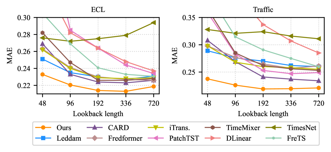
Figure 15: Performance change with increasing lookback lengths. The prediction length is $\tau=96$.

I.4 Training with less data

Training with less data reflects a model’s adaptability and learning efficacy. As shown in Figure 16, OLinear adapts well to decreasing training set sizes, from 100% down to 5%. Our model consistently outperforms others across all training ratios, highlighting its robustness to data-sparse conditions.

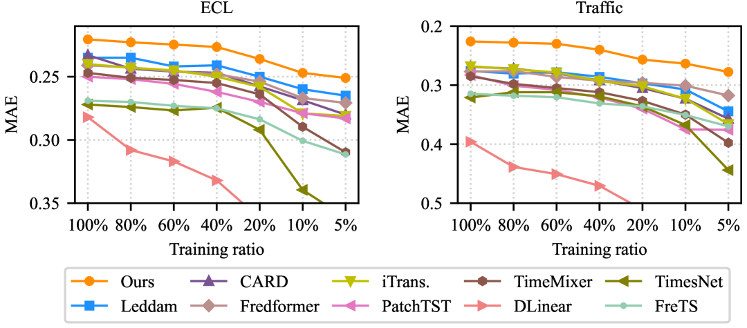
Figure 16: Performance change with less training data. The lookback and prediction lengths are set to 96. The Y-axis is inverted for clarity.

I.5 OLinear versus Timer

We further compare OLinear with the large pre-trained time series model Timer [Liu et al., 2024b] in terms of few-shot and zero-shot capabilities. As shown in Table 29, OLinear surprisingly achieves comparable performance to Timer [Liu et al., 2024b], despite not being pre-trained on large-scale datasets. When the full training set is used, OLinear outperforms the fine-tuned Timer on the ECL, Traffic, Weather, and PEMS datasets. Even when only 5% of training data are available, OLinear still performs better on the ETTm1 and ETTm2 datasets. For zero-shot learning, our model—trained on ETTh1/ETTm1/ETTm2—outperforms Timer on ETTh2/ETTm2/ETTm1, respectively. This phenomenon not only demonstrates OLinear’s strong generalization ability, but also suggests that large time series models are still in the early stages of development.

Table 29: Performance comparison with Timer on fine-tuning and zero-shot scenarios. MSEs are reported, with a prediction length of 96. Better results are highlighted in bold. For OLinear’s zero-shot performance, we adopt the $\mathrm{ETTh1}\leftrightarrow\mathrm{ETTh2}$ and $\mathrm{ETTm1}\leftrightarrow\mathrm{ETTm2}$ scheme (e.g., training on ETTh1 and evaluating on ETTh2, or vice versa).

Train. Ratio	100%		20%		5%		0% (Zero-shot)
Model	Ours	Timer	Ours	Timer	Ours	Timer	Ours	Timer-28B
pre-trained	No	UTSD-12G	No	UTSD-12G	No	UTSD-12G	ETT	UTSD+LOTSA
ETTh1	0.363	0.358	0.396	0.359	0.413	0.362	0.416	0.393
ETTh2	0.276	–	0.289	0.284	0.303	0.280	0.287	0.308
ETTm1	0.275	–	0.300	0.321	0.321	0.321	0.355	0.420
ETTm2	0.161	–	0.167	0.187	0.170	0.176	0.176	0.247
ECL	0.123	0.136	0.131	0.134	0.153	0.132	-	0.147
Traffic	0.338	0.351	0.371	0.352	0.419	0.361	-	0.414
Weather	0.144	0.154	0.156	0.151	0.168	0.151	-	0.243
PEMS03	0.103	0.118	0.116	0.116	0.226	0.125	-	-
PEMS04	0.086	0.107	0.195	0.120	0.542	0.135	-	-

I.6 Hyperparameter sensitivity

We evaluate the hyperparameter sensitivity of OLinear with respect to four key factors: the learning rate ($lr$), the number of blocks ($L$), the model dimension ($D$), and the embedding size ($d$). As shown in Figure 17, OLinear generally maintains stable performance across different choices of $lr$, $L$, and $D$, although each dataset exhibits its own preferences. Regarding the embedding size $d$, Table 30 indicates that $d=16$ represents a sweet spot, which we adopt as the default setting in our experiments.

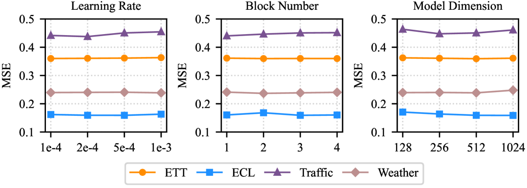
Figure 17: Hyperparameter sensitivity with respect to the learning rate $lr$, the number of blocks $L$, and the model dimension $D$. Average MSEs are reported across four prediction lengths $\tau\in\left\{96,192,336,720\right\}$. ETT denotes the average performance over four subsets: $\mathrm{ETT}\left\{\mathrm{h}1,\mathrm{h}2,\mathrm{m}1,\mathrm{m}2\right\}$. The lookback length $T$ is uniformly set as 96.

Table 30: Performance with various embedding size $d$ settings. In our main experiments, we set $d=16$ without specific statements.

Emb. size		1		4		8		16		32		64
Metric		MSE	MAE	MSE	MAE	MSE	MAE	MSE	MAE	MSE	MAE	MSE	MAE
ECL	96	0.133	0.223	0.132	0.221	0.132	0.221	0.131	0.221	0.131	0.221	0.131	0.221
	192	0.152	0.240	0.153	0.241	0.152	0.240	0.150	0.238	0.153	0.241	0.152	0.240
	336	0.166	0.256	0.169	0.257	0.165	0.255	0.165	0.254	0.165	0.255	0.168	0.258
	720	0.188	0.277	0.198	0.282	0.207	0.290	0.191	0.279	0.193	0.280	0.200	0.286
	Avg	0.159	0.249	0.163	0.250	0.164	0.252	0.159	0.248	0.161	0.249	0.163	0.251
Traffic	96	0.398	0.230	0.411	0.227	0.403	0.226	0.398	0.226	0.402	0.226	0.404	0.226
	192	0.425	0.243	0.433	0.241	0.443	0.241	0.439	0.241	0.436	0.241	0.435	0.242
	336	0.450	0.251	0.462	0.250	0.465	0.249	0.464	0.250	0.460	0.251	0.459	0.254
	720	0.496	0.269	0.518	0.269	0.520	0.270	0.502	0.270	0.507	0.274	0.515	0.275
	Avg	0.442	0.248	0.456	0.247	0.458	0.246	0.451	0.247	0.451	0.248	0.453	0.249
Solar-Energy	96	0.180	0.194	0.179	0.193	0.180	0.191	0.179	0.191	0.177	0.190	0.182	0.192
	192	0.212	0.216	0.211	0.214	0.209	0.213	0.209	0.213	0.212	0.213	0.211	0.214
	336	0.234	0.233	0.232	0.230	0.230	0.230	0.231	0.229	0.231	0.230	0.233	0.231
	720	0.244	0.238	0.241	0.236	0.241	0.235	0.241	0.236	0.242	0.236	0.243	0.238
	Avg	0.217	0.220	0.216	0.218	0.215	0.217	0.215	0.217	0.215	0.217	0.217	0.219
Weather	96	0.152	0.189	0.158	0.192	0.150	0.187	0.152	0.189	0.152	0.190	0.157	0.194
	192	0.203	0.238	0.200	0.234	0.207	0.242	0.207	0.243	0.202	0.238	0.205	0.239
	336	0.261	0.282	0.259	0.280	0.259	0.280	0.261	0.282	0.263	0.282	0.269	0.287
	720	0.342	0.337	0.343	0.338	0.343	0.337	0.344	0.337	0.350	0.339	0.344	0.336
	Avg	0.240	0.261	0.240	0.261	0.240	0.261	0.241	0.262	0.242	0.262	0.244	0.264
ILI	3	0.487	0.355	0.545	0.380	0.500	0.353	0.468	0.349	0.515	0.362	0.486	0.352
	6	0.915	0.515	1.021	0.533	0.890	0.506	0.923	0.516	0.914	0.515	1.059	0.558
	9	1.301	0.662	1.363	0.666	1.376	0.667	1.289	0.655	1.265	0.644	1.264	0.645
	12	1.638	0.783	1.693	0.788	1.810	0.799	1.698	0.791	1.619	0.769	1.747	0.773
	Avg	1.085	0.579	1.155	0.592	1.144	0.581	1.094	0.578	1.078	0.572	1.139	0.582
PEMS03	12	0.060	0.159	0.060	0.159	0.060	0.159	0.060	0.159	0.061	0.160	0.059	0.158
	24	0.077	0.179	0.078	0.179	0.078	0.180	0.078	0.179	0.077	0.179	0.077	0.179
	48	0.107	0.213	0.106	0.211	0.106	0.211	0.104	0.210	0.106	0.211	0.105	0.210
	96	0.146	0.253	0.143	0.248	0.141	0.248	0.140	0.247	0.140	0.247	0.143	0.248
	Avg	0.097	0.201	0.097	0.199	0.096	0.200	0.095	0.199	0.096	0.199	0.096	0.199
1st Count		9	4	4	8	9	12	12	14	8	12	4	7

I.7 More metrics

We further conduct a comprehensive evaluation of forecasting performance using three scale-free metrics: the Coefficient of Determination ($R^{2}$), the Pearson Correlation Coefficient ($r$), and the Mean Absolute Scaled Error (MASE), which are defined as follows:

$$R^{2} =\frac{1}{N}\sum_{n=1}^{N}\left(1-\frac{\left|\hat{\mathbf{Y}}_{n:}-\mathbf{Y}_{n:}\right|^{2}_{2}}{\left|\mathbf{Y}_{n:}-\overline{\mathbf{Y}_{n:}}\right|^{2}_{2}}\right),$$ (22)

$$r =\frac{1}{N}\sum_{n=1}^{N}\frac{{\textstyle\sum_{t=1}^{\tau}}\left(\hat{\mathbf{Y}}_{n,t}-\overline{\hat{\mathbf{Y}}_{n:}}\right)\left(\mathbf{Y}_{n,t}-\overline{\mathbf{Y}_{n:}}\right)}{\sqrt{{\textstyle\sum_{t=1}^{\tau}}\left(\hat{\mathbf{Y}}_{n,t}-\overline{\hat{\mathbf{Y}}_{n:}}\right)^{2}}\sqrt{{\textstyle\sum_{t=1}^{\tau}}\left(\mathbf{Y}_{n,t}-\overline{\mathbf{Y}_{n:}}\right)^{2}}},$$

$$\mathrm{MASE} =\frac{1}{N}\sum_{n=1}^{N}\frac{\frac{1}{\tau}\left\|\hat{\mathbf{Y}}_{n:}-\mathbf{Y}_{n:}\right\|_{1}}{\frac{1}{\tau-1}{\textstyle\sum_{t=1}^{\tau-1}\left|\mathbf{Y}_{n,t}-\mathbf{Y}_{t-1,n}\right|}}.$$

Here $\mathbf{Y}_{n:}$ and $\hat{\mathbf{Y}}_{n:}$ denote the $n$-th variate of the ground truth $\mathbf{Y}$ and the prediction $\hat{\mathbf{Y}}$, respectively. $\mathbf{Y}_{n,t}$ refers to the $t$-th timestep of the $n$-th variate, and $\overline{(\cdot)}$ represents the mean.

As shown in Table 31, OLinear consistently achieves state-of-the-art performance on these metrics. For example, it an average Pearson correlation coefficient of $r=0.903$ on the ECL dataset, indicating strong alignment between predictions and ground truth. On the Traffic dataset, OLinear achieves a MASE of 0.764, outperforming the second-best model, CARD [Wang et al., 2024b], by a notable margin of 11.4%.

Table 31: Forecasting performance on the scale-free metrics: Coefficient of Determination ($R^{2}$), Pearson Correlation Coefficient ($r$), and MASE. The symbols $\downarrow$ and $\uparrow$ indicate that lower and higher values are better, respectively. The best and second-best results are highlighted in bold and underlined, respectively. The lookback length $T$ is uniformly set as 96.

Model		OLinear (Ours)			Leddam 2024			CARD 2024b			iTrans. 2024a			TimeMixer 2024a
Metric		$R^{2}$ ($\uparrow$)	$r$ ($\uparrow$)	MASE ($\downarrow$)	$R^{2}$ ($\uparrow$)	$r$ ($\uparrow$)	MASE ($\downarrow$)	$R^{2}$ ($\uparrow$)	$r$ ($\uparrow$)	MASE ($\downarrow$)	$R^{2}$ ($\uparrow$)	$r$ ($\uparrow$)	MASE ($\downarrow$)	$R^{2}$ ($\uparrow$)	$r$ ($\uparrow$)	MASE ($\downarrow$)
ECL	96	0.640	0.916	0.902	0.527	0.911	0.964	0.533	0.905	0.975	0.550	0.907	0.990	0.456	0.897	1.022
	192	0.638	0.908	0.983	0.593	0.902	1.041	0.547	0.899	1.028	0.590	0.900	1.057	0.575	0.893	1.076
	336	0.710	0.901	1.061	0.670	0.893	1.134	0.678	0.891	1.113	0.678	0.893	1.133	0.640	0.886	1.155
	720	0.701	0.889	1.174	0.661	0.882	1.251	0.653	0.877	1.273	0.638	0.872	1.315	0.634	0.871	1.314
	Avg	0.672	0.903	1.030	0.613	0.897	1.098	0.603	0.893	1.097	0.614	0.893	1.124	0.576	0.887	1.142
Traffic	96	0.737	0.899	0.729	0.681	0.885	0.909	0.690	0.882	0.855	0.690	0.889	0.860	0.640	0.888	0.979
	192	0.719	0.884	0.756	0.666	0.865	0.949	0.683	0.869	0.856	0.689	0.877	0.879	0.660	0.862	0.959
	336	0.730	0.875	0.758	0.707	0.867	0.897	0.702	0.862	0.843	0.713	0.867	0.883	0.685	0.852	0.960
	720	0.703	0.860	0.815	0.687	0.853	0.947	0.679	0.848	0.894	0.693	0.857	0.913	0.672	0.842	0.986
	Avg	0.722	0.879	0.764	0.685	0.868	0.926	0.689	0.865	0.862	0.696	0.873	0.884	0.664	0.861	0.971
Model		FilterNet 2024a			FITS 2024			DLinear 2023			PatchTST 2023			TimesNet 2023b
Metric		$R^{2}$ ($\uparrow$)	$r$ ($\uparrow$)	MASE ($\downarrow$)	$R^{2}$ ($\uparrow$)	$r$ ($\uparrow$)	MASE ($\downarrow$)	$R^{2}$ ($\uparrow$)	$r$ ($\uparrow$)	MASE ($\downarrow$)	$R^{2}$ ($\uparrow$)	$r$ ($\uparrow$)	MASE ($\downarrow$)	$R^{2}$ ($\uparrow$)	$r$ ($\uparrow$)	MASE ($\downarrow$)
ECL	96	0.537	0.905	0.996	0.352	0.883	1.144	0.120	0.870	1.300	0.426	0.890	1.119	0.405	0.892	1.118
	192	0.576	0.898	1.052	0.446	0.880	1.153	0.215	0.867	1.312	0.509	0.887	1.140	0.503	0.885	1.195
	336	0.670	0.891	1.139	0.588	0.873	1.229	0.247	0.858	1.387	0.604	0.880	1.216	0.592	0.875	1.262
	720	0.628	0.875	1.328	0.593	0.858	1.376	0.148	0.844	1.536	0.605	0.864	1.371	0.603	0.864	1.388
	Avg	0.603	0.892	1.129	0.495	0.873	1.225	0.182	0.860	1.384	0.536	0.880	1.211	0.526	0.879	1.241
Traffic	96	0.637	0.876	0.987	0.458	0.811	1.284	0.441	0.811	1.346	0.668	0.880	0.903	0.625	0.877	1.023
	192	0.665	0.867	0.950	0.542	0.814	1.151	0.551	0.815	1.189	0.677	0.871	0.887	0.635	0.867	1.009
	336	0.696	0.861	0.930	0.582	0.810	1.119	0.582	0.810	1.167	0.700	0.863	0.874	0.654	0.852	1.079
	720	0.678	0.847	0.982	0.568	0.794	1.169	0.564	0.794	1.224	0.681	0.850	0.925	0.661	0.850	1.047
	Avg	0.669	0.862	0.962	0.537	0.807	1.181	0.535	0.808	1.232	0.682	0.866	0.897	0.644	0.862	1.040

I.8 Less training data to compute Q matrices

To evaluate the amount of training data required for computing the orthogonal transformation matrices $\mathbf{Q}_{i}$ and $\mathbf{Q}_{o}$, we conduct experiments using only partial data of the training set. As shown in Table 32, OLinear exhibits strong robustness, with minimal performance variation across different data proportions. This property not only enables more efficient preprocessing before training, but also ensures robust performance in few-shot learning scenarios (see Appendix LABEL:few-shot).

Table 32: Forecasting performance with orthogonal matrices computed from varying proportions of the training data, denoted as ‘Q_ratio’. All experiments are trained on the full training set.

Q_ratio		100%		80%		60%		40%		20%		10%
Metric		MSE	MAE	MSE	MAE	MSE	MAE	MSE	MAE	MSE	MAE	MSE	MAE
	96	0.131	0.221	0.131	0.221	0.131	0.221	0.131	0.221	0.130	0.221	0.131	0.221
	192	0.150	0.238	0.155	0.243	0.152	0.239	0.153	0.240	0.151	0.240	0.152	0.240
	336	0.165	0.254	0.169	0.257	0.164	0.253	0.166	0.255	0.165	0.254	0.166	0.255
	720	0.191	0.279	0.193	0.284	0.188	0.277	0.193	0.284	0.193	0.280	0.189	0.278
ECL	Avg	0.159	0.248	0.162	0.251	0.159	0.247	0.161	0.250	0.160	0.248	0.159	0.248
	96	0.398	0.226	0.403	0.226	0.403	0.227	0.401	0.226	0.404	0.226	0.402	0.226
	192	0.439	0.241	0.436	0.240	0.434	0.240	0.432	0.240	0.434	0.240	0.431	0.240
	336	0.464	0.250	0.461	0.250	0.462	0.250	0.463	0.250	0.459	0.250	0.465	0.250
	720	0.502	0.270	0.499	0.271	0.499	0.271	0.501	0.271	0.502	0.271	0.512	0.271
Traffic	Avg	0.451	0.247	0.450	0.247	0.449	0.247	0.449	0.247	0.450	0.247	0.453	0.247
	96	0.153	0.190	0.150	0.188	0.153	0.191	0.153	0.190	0.154	0.191	0.149	0.187
	192	0.200	0.235	0.202	0.237	0.204	0.239	0.203	0.238	0.202	0.237	0.203	0.239
	336	0.258	0.280	0.260	0.280	0.260	0.281	0.264	0.284	0.260	0.281	0.259	0.281
	720	0.337	0.333	0.339	0.333	0.338	0.332	0.337	0.332	0.335	0.330	0.339	0.332
Weather	Avg	0.237	0.260	0.238	0.259	0.239	0.261	0.239	0.261	0.238	0.260	0.237	0.260
	12	0.060	0.159	0.060	0.159	0.060	0.159	0.060	0.159	0.061	0.160	0.060	0.159
	24	0.078	0.179	0.077	0.179	0.077	0.180	0.077	0.179	0.077	0.180	0.077	0.180
	48	0.104	0.210	0.105	0.210	0.104	0.210	0.104	0.210	0.104	0.210	0.105	0.210
	96	0.140	0.247	0.141	0.248	0.142	0.248	0.141	0.248	0.143	0.249	0.140	0.249
PEMS03	Avg	0.095	0.199	0.096	0.199	0.096	0.199	0.095	0.199	0.096	0.199	0.095	0.199
	3	0.036	0.092	0.036	0.092	0.036	0.092	0.036	0.093	0.036	0.093	0.036	0.093
	6	0.049	0.117	0.049	0.117	0.049	0.117	0.049	0.117	0.049	0.117	0.049	0.118
	9	0.062	0.137	0.062	0.137	0.062	0.137	0.062	0.137	0.062	0.137	0.062	0.137
	12	0.073	0.154	0.073	0.154	0.073	0.154	0.073	0.154	0.073	0.154	0.073	0.154
NASDAQ	Avg	0.055	0.125	0.055	0.125	0.055	0.125	0.055	0.125	0.055	0.125	0.055	0.125
	24	0.320	0.302	0.319	0.302	0.319	0.301	0.319	0.302	0.320	0.302	0.320	0.302
	36	0.334	0.315	0.334	0.315	0.334	0.315	0.334	0.315	0.334	0.315	0.334	0.316
	48	0.347	0.327	0.347	0.327	0.347	0.327	0.347	0.327	0.347	0.327	0.347	0.328
	60	0.358	0.337	0.358	0.337	0.358	0.337	0.358	0.337	0.358	0.337	0.358	0.337
CarSales	Avg	0.340	0.320	0.339	0.320	0.339	0.320	0.340	0.320	0.340	0.320	0.340	0.320

Appendix J More ablation studies

J.1 Ablations on NormLin design

In the NormLin layer, the $\mathrm{Softplus}$ function followed by L1 row-wise normalization is applied to the learnable weight matrix $\mathbf{W}$ to produce attention-like matrices, i.e., $\mathrm{RowNorm}_{\mathrm{L1}}(\mathrm{Softplus}(\mathbf{W}))$. To assess the effects of different transformations and normalization strategies, we consider transformation functions from the set $\{\mathrm{Softplus},\mathrm{Identity},\mathrm{Softmax},\mathrm{Sigmoid},\mathrm{ReLU}\}$ and and normalization methods from ${\mathrm{L1},\mathrm{L2}}$ (all applied row-wise). Here, $\mathrm{Identity}$ denotes no transformation.

As shown in Table 33, the combination ‘$\mathrm{Softplus}$ + $\mathrm{L1}$’ yields the best performance among the 10 candidates. On average, L1 normalization leads to a 10% performance improvement over L2, while $\mathrm{Softplus}$ slightly outperforms $\mathrm{Softmax}$ and other transformation functions.

Table 33: Ablation study on transformation functions and normalization methods in NormLin. For S1 and S2, the prediction lengths are $\left\{3,6,9,12\right\}$ and $\left\{24,36,48,60\right\}$, respectively.

Fun.	Norm	Hor.	ECL		Traffic		Solar		PEMS03		Weather		NASDAQ (S1)		ILI (S2)
		H1	0.131	0.221	0.398	0.226	0.179	0.191	0.060	0.159	0.153	0.190	0.036	0.092	1.737	0.800
		H2	0.150	0.238	0.439	0.241	0.209	0.213	0.078	0.179	0.200	0.235	0.049	0.117	1.714	0.795
		H3	0.165	0.254	0.464	0.250	0.231	0.229	0.104	0.210	0.258	0.280	0.062	0.137	1.821	0.804
		H4	0.191	0.279	0.502	0.270	0.241	0.236	0.140	0.247	0.337	0.333	0.073	0.154	1.785	0.810
Softplus	L1	Avg	0.159	0.248	0.451	0.247	0.215	0.217	0.095	0.199	0.237	0.260	0.055	0.125	1.764	0.802
		H1	0.140	0.229	0.455	0.233	0.182	0.193	0.062	0.161	0.154	0.191	0.036	0.093	1.783	0.807
		H2	0.157	0.245	0.486	0.246	0.216	0.215	0.078	0.179	0.203	0.240	0.049	0.117	1.844	0.810
		H3	0.170	0.260	0.506	0.255	0.239	0.233	0.103	0.208	0.267	0.285	0.061	0.137	1.909	0.826
		H4	0.200	0.287	0.551	0.276	0.506	0.255	0.143	0.250	0.350	0.339	0.073	0.154	1.841	0.830
Identity	L1	Avg	0.167	0.255	0.499	0.252	0.285	0.224	0.096	0.199	0.243	0.264	0.055	0.125	1.844	0.818
		H1	0.131	0.221	0.398	0.226	0.179	0.192	0.061	0.160	0.150	0.187	0.036	0.092	1.707	0.800
		H2	0.155	0.242	0.441	0.241	0.209	0.213	0.077	0.179	0.202	0.237	0.049	0.117	1.886	0.828
		H3	0.167	0.255	0.467	0.250	0.232	0.229	0.107	0.211	0.259	0.280	0.062	0.138	1.820	0.803
		H4	0.199	0.286	0.504	0.270	0.241	0.236	0.139	0.247	0.335	0.332	0.073	0.154	1.795	0.814
Softmax	L1	Avg	0.163	0.251	0.452	0.247	0.215	0.217	0.096	0.199	0.236	0.259	0.055	0.125	1.802	0.811
		H1	0.131	0.221	0.398	0.226	0.178	0.191	0.061	0.159	0.152	0.189	0.035	0.093	1.742	0.799
		H2	0.150	0.238	0.439	0.241	0.209	0.213	0.077	0.179	0.203	0.238	0.049	0.117	1.719	0.797
		H3	0.167	0.256	0.464	0.250	0.231	0.229	0.106	0.211	0.262	0.283	0.062	0.137	1.826	0.804
		H4	0.199	0.285	0.500	0.270	0.241	0.236	0.139	0.248	0.338	0.332	0.073	0.154	1.780	0.808
Sigmoid	L1	Avg	0.161	0.250	0.450	0.247	0.215	0.217	0.096	0.199	0.239	0.260	0.055	0.125	1.767	0.802
		H1	0.132	0.222	0.398	0.226	0.179	0.191	0.061	0.160	0.153	0.189	0.036	0.092	1.711	0.799
		H2	0.153	0.241	0.443	0.241	0.210	0.213	0.078	0.179	0.202	0.238	0.049	0.117	1.721	0.795
		H3	0.170	0.259	0.467	0.250	0.231	0.229	0.106	0.211	0.264	0.285	0.062	0.138	1.816	0.804
		H4	0.197	0.285	0.507	0.271	0.241	0.236	0.143	0.248	0.338	0.335	0.073	0.154	1.790	0.812
ReLU	L1	Avg	0.163	0.251	0.454	0.247	0.215	0.217	0.097	0.199	0.239	0.262	0.055	0.125	1.759	0.802
		H1	0.192	0.285	0.613	0.313	0.234	0.244	0.095	0.199	0.151	0.188	0.036	0.093	1.928	0.852
		H2	0.194	0.288	0.640	0.325	0.280	0.267	0.121	0.221	0.203	0.238	0.050	0.119	1.929	0.837
		H3	0.202	0.297	0.653	0.329	0.323	0.288	0.174	0.265	0.259	0.281	0.063	0.139	1.845	0.806
		H4	0.236	0.322	0.683	0.344	0.337	0.292	0.264	0.331	0.339	0.335	0.073	0.154	1.794	0.813
Softplus	L2	Avg	0.206	0.298	0.647	0.328	0.293	0.273	0.163	0.254	0.238	0.260	0.055	0.126	1.874	0.827
		H1	0.139	0.230	0.456	0.238	0.187	0.198	0.063	0.163	0.151	0.189	0.036	0.092	1.718	0.795
		H2	0.159	0.249	0.516	0.251	0.221	0.219	0.080	0.184	0.201	0.238	0.050	0.118	1.855	0.812
		H3	0.171	0.261	0.529	0.261	0.239	0.234	0.112	0.217	0.266	0.284	0.062	0.137	1.947	0.831
		H4	0.215	0.298	0.573	0.288	0.248	0.239	0.153	0.258	0.347	0.339	0.073	0.154	1.832	0.829
Identity	L2	Avg	0.171	0.259	0.518	0.259	0.224	0.222	0.102	0.205	0.241	0.262	0.055	0.125	1.838	0.817
		H1	0.183	0.278	0.612	0.312	0.233	0.242	0.096	0.199	0.153	0.190	0.036	0.093	1.876	0.837
		H2	0.192	0.286	0.641	0.325	0.266	0.256	0.118	0.219	0.199	0.235	0.050	0.119	1.875	0.825
		H3	0.202	0.297	0.653	0.330	0.313	0.280	0.174	0.265	0.259	0.282	0.063	0.139	1.823	0.803
		H4	0.226	0.316	0.686	0.346	0.336	0.292	0.268	0.334	0.337	0.333	0.073	0.154	1.798	0.814
Softmax	L2	Avg	0.201	0.294	0.648	0.328	0.287	0.267	0.164	0.254	0.237	0.260	0.055	0.126	1.843	0.820
		H1	0.193	0.285	0.613	0.313	0.234	0.244	0.096	0.200	0.149	0.187	0.036	0.094	1.993	0.861
		H2	0.206	0.296	0.640	0.324	0.279	0.267	0.119	0.220	0.204	0.239	0.050	0.119	1.762	0.807
		H3	0.201	0.296	0.653	0.329	0.324	0.288	0.175	0.267	0.262	0.284	0.063	0.139	1.866	0.811
		H4	0.256	0.334	0.684	0.345	0.336	0.291	0.265	0.332	0.337	0.333	0.073	0.155	1.797	0.813
Sigmoid	L2	Avg	0.214	0.302	0.647	0.328	0.293	0.272	0.164	0.255	0.238	0.261	0.056	0.127	1.854	0.823
		H1	0.181	0.277	0.612	0.312	0.231	0.241	0.095	0.197	0.153	0.190	0.036	0.093	1.860	0.838
		H2	0.190	0.284	0.640	0.325	0.265	0.255	0.118	0.219	0.201	0.237	0.050	0.119	1.900	0.833
		H3	0.200	0.295	0.653	0.329	0.309	0.278	0.176	0.268	0.260	0.282	0.063	0.139	1.803	0.800
		H4	0.232	0.320	0.686	0.346	0.335	0.291	0.263	0.330	0.336	0.332	0.073	0.154	1.798	0.813
ReLU	L2	Avg	0.201	0.294	0.648	0.328	0.285	0.266	0.163	0.254	0.237	0.260	0.055	0.126	1.840	0.821

J.2 Pre- and post-linear layers in NormLin module

In CSL, the pre- and post-linear layers, named based on their positions in the execution sequence, are applied around the NormLin layer (see Equation 4): $\mathrm{Post\_Lin}\left(\mathrm{NormLin}\left(\mathrm{Pre\_Lin}(\cdot)\right)\right)$.

We conduct ablation studies to evaluate the contributions of these two layers. As shown in Table 34, incorporating both pre- and post-linear layers yields an average performance gain of 6% compared to the variant without them, highlighting their effectiveness in refining inputs for multivariate correlation modeling and downstream series representation learning.

Table 34: Ablation study on pre- and post-linear layers around the NormLin layer. ‘Hor.’ denotes prediction horizons. For S1 and S2, the prediction lengths are $\left\{3,6,9,12\right\}$ and $\left\{24,36,48,60\right\}$, respectively.

			ECL		Traffic		Solar		PEMS03		Weather		NASDAQ (S1)		ILI (S2)		Wiki (S1)		ETTm1
Pre_Lin	Post_Lin	Hor.	MSE	MAE	MSE	MAE	MSE	MAE	MSE	MAE	MSE	MAE	MSE	MAE	MSE	MAE	MSE	MAE	MSE	MAE
		H1	0.135	0.229	0.474	0.253	0.192	0.206	0.065	0.167	0.159	0.195	0.040	0.104	1.744	0.861	6.184	0.372	0.320	0.352
		H2	0.153	0.246	0.492	0.264	0.225	0.228	0.085	0.191	0.207	0.241	0.053	0.126	1.970	0.891	6.471	0.387	0.373	0.384
		H3	0.168	0.264	0.511	0.273	0.247	0.244	0.125	0.233	0.264	0.285	0.065	0.146	2.153	0.892	6.673	0.403	0.401	0.400
		H4	0.204	0.297	0.555	0.294	0.255	0.247	0.178	0.281	0.342	0.336	0.077	0.162	2.091	0.890	6.846	0.410	0.461	0.435
✗	✗	Avg	0.165	0.259	0.508	0.271	0.230	0.231	0.113	0.218	0.243	0.264	0.058	0.134	1.989	0.883	6.543	0.393	0.389	0.393
		H1	0.131	0.222	0.403	0.228	0.179	0.192	0.061	0.161	0.155	0.192	0.036	0.094	1.926	0.858	6.176	0.368	0.303	0.334
		H2	0.151	0.240	0.434	0.242	0.210	0.213	0.077	0.180	0.205	0.240	0.049	0.118	1.796	0.827	6.447	0.384	0.356	0.364
		H3	0.166	0.256	0.457	0.251	0.231	0.230	0.107	0.212	0.262	0.282	0.062	0.137	1.960	0.833	6.650	0.399	0.389	0.387
		H4	0.211	0.298	0.500	0.272	0.243	0.236	0.146	0.253	0.352	0.340	0.073	0.155	1.799	0.811	6.839	0.406	0.452	0.426
✗	✔	Avg	0.165	0.254	0.448	0.248	0.216	0.218	0.098	0.201	0.243	0.263	0.055	0.126	1.870	0.832	6.528	0.389	0.375	0.378
		H1	0.131	0.222	0.404	0.228	0.178	0.192	0.061	0.160	0.154	0.192	0.036	0.094	1.924	0.858	6.175	0.368	0.303	0.334
		H2	0.155	0.243	0.434	0.242	0.211	0.214	0.077	0.180	0.204	0.239	0.049	0.118	1.796	0.828	6.448	0.385	0.356	0.364
		H3	0.165	0.255	0.457	0.251	0.231	0.230	0.107	0.212	0.263	0.282	0.062	0.137	1.959	0.833	6.649	0.399	0.389	0.387
		H4	0.209	0.293	0.499	0.272	0.242	0.236	0.144	0.252	0.344	0.339	0.073	0.155	1.799	0.811	6.839	0.406	0.452	0.426
✔	✗	Avg	0.165	0.253	0.448	0.248	0.215	0.218	0.097	0.201	0.241	0.263	0.055	0.126	1.869	0.832	6.528	0.389	0.375	0.378
		H1	0.131	0.221	0.398	0.226	0.179	0.191	0.060	0.159	0.152	0.189	0.036	0.092	1.737	0.800	6.161	0.368	0.302	0.334
		H2	0.150	0.238	0.439	0.241	0.209	0.213	0.078	0.179	0.207	0.243	0.049	0.117	1.714	0.795	6.453	0.385	0.357	0.364
		H3	0.165	0.254	0.464	0.250	0.231	0.229	0.104	0.210	0.261	0.282	0.062	0.137	1.821	0.804	6.666	0.398	0.387	0.385
		H4	0.191	0.279	0.502	0.270	0.241	0.236	0.140	0.247	0.344	0.337	0.073	0.154	1.785	0.810	6.834	0.406	0.452	0.426
✔	✔	Avg	0.159	0.248	0.451	0.247	0.215	0.217	0.095	0.199	0.241	0.263	0.055	0.125	1.764	0.802	6.528	0.389	0.374	0.377

J.3 Ablations on Q matrices

The effectiveness of OrthoTrans has been demonstrated in Tables 4 and 5. To further analyze the individual contributions of $\mathbf{Q}_{i}$ and $\mathbf{Q}_{o}$, we conduct ablation studies on these transformation matrices.

As shown in Table 35, using both $\mathbf{Q}_{i}$ and $\mathbf{Q}_{o}$ achieves the best performance—reducing the average MSE by 5.3% compared to the baseline without transformations, by 4.4% compared to using $\mathbf{Q}_{o}$ only, and by 0.8% compared to using $\mathbf{Q}_{i}$ only. Notably, the variant using only $\mathbf{Q}_{i}$ outperforms the one using only $\mathbf{Q}_{o}$, highlighting the critical role of temporal decorrelation in effective encoding and representation learning.

Table 35: Ablation study on $\mathbf{Q}_{i}$ and $\mathbf{Q}_{o}$. ‘Hor.’ denotes prediction horizons. For S1 and S2, the prediction lengths are $\{3,6,9,12\}$ and $\{24,36,48,60\}$, respectively.

			ECL		Solar-Energy		PEMS03		PEMS08		NASDAQ (S1)		ILI (S2)		COVID-19 (S2)		Exchange
$\mathbf{Q}_{i}$	$\mathbf{Q}_{o}$	Hor.	MSE	MAE	MSE	MAE	MSE	MAE	MSE	MAE	MSE	MAE	MSE	MAE	MSE	MAE	MSE	MAE
		H1	0.134	0.224	0.186	0.199	0.063	0.163	0.070	0.162	0.036	0.093	1.891	0.847	4.841	1.284	0.083	0.203
		H2	0.156	0.245	0.221	0.220	0.080	0.184	0.091	0.183	0.050	0.119	1.889	0.844	7.828	1.757	0.173	0.295
		H3	0.167	0.257	0.244	0.237	0.117	0.222	0.128	0.216	0.063	0.139	1.854	0.811	10.153	2.003	0.335	0.416
		H4	0.194	0.282	0.256	0.244	0.165	0.266	0.231	0.262	0.074	0.156	1.802	0.816	12.603	2.232	0.846	0.692
✗	✗	Avg	0.163	0.252	0.227	0.225	0.106	0.209	0.130	0.206	0.056	0.127	1.859	0.829	8.856	1.819	0.359	0.401
		H1	0.132	0.223	0.186	0.198	0.062	0.162	0.069	0.162	0.036	0.093	1.844	0.830	4.645	1.260	0.083	0.203
		H2	0.153	0.243	0.219	0.219	0.079	0.183	0.092	0.183	0.050	0.119	1.779	0.811	8.137	1.798	0.173	0.295
		H3	0.167	0.258	0.246	0.238	0.115	0.221	0.132	0.217	0.063	0.139	1.854	0.809	10.054	1.990	0.334	0.416
		H4	0.194	0.285	0.255	0.244	0.164	0.267	0.216	0.261	0.074	0.156	1.787	0.813	12.000	2.189	0.848	0.693
✗	✔	Avg	0.161	0.252	0.226	0.225	0.105	0.208	0.127	0.206	0.056	0.127	1.816	0.816	8.709	1.809	0.359	0.401
		H1	0.131	0.221	0.179	0.191	0.061	0.159	0.068	0.159	0.036	0.092	1.897	0.847	4.957	1.330	0.082	0.200
		H2	0.154	0.241	0.210	0.212	0.076	0.178	0.087	0.177	0.049	0.117	1.886	0.836	7.100	1.654	0.172	0.293
		H3	0.165	0.254	0.230	0.229	0.105	0.211	0.121	0.204	0.062	0.137	1.809	0.802	10.224	2.009	0.332	0.414
		H4	0.188	0.279	0.241	0.235	0.142	0.249	0.182	0.238	0.073	0.154	1.784	0.811	11.779	2.160	0.837	0.688
✔	✗	Avg	0.159	0.249	0.215	0.217	0.096	0.199	0.114	0.194	0.055	0.125	1.844	0.824	8.515	1.788	0.355	0.399
		H1	0.131	0.221	0.179	0.191	0.060	0.159	0.068	0.159	0.036	0.092	1.737	0.800	4.474	1.180	0.082	0.200
		H2	0.150	0.238	0.209	0.213	0.078	0.179	0.089	0.178	0.049	0.117	1.714	0.795	7.241	1.670	0.171	0.293
		H3	0.165	0.254	0.231	0.229	0.104	0.210	0.123	0.204	0.062	0.137	1.821	0.804	10.076	1.985	0.331	0.414
		H4	0.191	0.279	0.241	0.236	0.140	0.247	0.173	0.236	0.073	0.154	1.785	0.810	12.079	2.182	0.837	0.688
✔	✔	Avg	0.159	0.248	0.215	0.217	0.095	0.199	0.113	0.194	0.055	0.125	1.764	0.802	8.467	1.754	0.355	0.399

J.4 Swapping Q matrices

Table 36 reports the forecasting performance when both training and testing are conducted using Q matrices ($\mathbf{Q}_{i}$ and $\mathbf{Q}_{o}$) derived from different datasets. As shown, using the Q matrices from the same dataset yields the best performance, highlighting the importance of incorporating dataset-specific temporal correlation information in time series forecasting.

Table 36: Forecasting performance when both training and testing use Q matrices $\mathbf{Q}_{i}$ and $\mathbf{Q}_{o}$ from different datasets. $\mathcal{A}\to\mathcal{B}$ indicates that the Q matrices computed from dataset $\mathcal{A}$ are applied in experiments on dataset $\mathcal{B}$.

Setting	ILI→ILI		Power→ILI		Web→ILI
Metric	MSE	MAE	MSE	MAE	MSE	MAE
24	1.737	0.800	1.846	0.830	1.887	0.842
36	1.714	0.795	1.721	0.801	1.743	0.807
48	1.821	0.804	1.849	0.810	1.875	0.817
60	1.785	0.810	1.824	0.814	1.815	0.813
Avg	1.764	0.802	1.810	0.814	1.830	0.820
Setting	ILI→Power		Power→Power		Web→Power
Metric	MSE	MAE	MSE	MAE	MSE	MAE
24	1.391	0.895	1.343	0.870	1.393	0.889
36	1.457	0.902	1.445	0.903	1.493	0.915
48	1.612	0.972	1.559	0.946	1.680	0.997
60	1.733	1.035	1.602	0.971	1.773	1.048
Avg	1.548	0.951	1.487	0.922	1.585	0.962
Setting	ILI→Web		Power→Web		Web→Web
Metric	MSE	MAE	MSE	MAE	MSE	MAE
24	0.208	0.319	0.185	0.306	0.186	0.306
36	0.285	0.369	0.289	0.364	0.272	0.356
48	0.377	0.403	0.400	0.427	0.365	0.391
60	0.480	0.476	0.467	0.466	0.486	0.481
Avg	0.337	0.391	0.335	0.391	0.327	0.383

Appendix K Model efficiency

As a linear model, OLinear achieves remarkable training and inference efficiency while delivering state-of-the-art forecasting performance. Figure 3 shows that OLinear achieves better efficiency than Transformer-based forecasters, benefiting from its relatively simple architecture. Detailed resource consumption for both training and inference is summarized in Table 37. Moreover, Table 38 presents the efficiency differences before and after applying the NormLin module to Transformer-based forecasters.

Table 37: Training and inference resource footprint for OLinear and baseline forecasters. ‘T.T.’, ‘T.M.’, ‘I.T.’ and ‘I.M.’ denote training time, training GPU memory usage, inference time, and inference GPU memory usage, respectively. All experiments use a lookback/prediction of 96 and a batch size of 16. To ensure a fair comparison, the number of layers (or blocks) is fixed at 2, except for DLinear, which employs only 1 linear layer. ‘OL’ refers to OLinear. ‘OOM’ indicates that the experiment runs out of memory on a 24 GB GPU.

Model		OL (Ours)	OL-C (Ours)	Leddam 2024	CARD 2024b	Fredformer 2024	iTrans. 2024a	TimeMix.++ 2025a	TimeMix. 2024a	Dlinear 2023	TimesNet 2023b	PatchTST 2023	FreTS 2023
ETT	Params(M)	4.52	4.52	8.55	0.03	8.59	4.83	1.19	0.08	0.02	299.94	3.76	0.42
	FLOPs(M)	33.74	33.74	111.54	1.41	135.01	33.99	1396.90	10.72	0.13	289708	272.20	2.94
	T.T. (ms/iter)	8.09	7.26	25.02	29.10	26.48	10.11	74.74	27.99	1.42	501.98	8.37	3.63
	T.M.(GB)	0.20	0.2	0.18	0.03	0.24	0.21	0.27	0.05	0.02	5.80	0.14	0.03
	I.T.(ms/iter)	1.19	1.09	2.62	4.05	3.73	1.72	28.15	3.86	0.21	155.97	1.38	0.49
	I.M. (MB)	156.41	156.41	51.04	11.02	78.04	156.00	149.58	18.06	8.48	1396.24	51.83	14.47
ECL	Params(M)	4.79	4.58	8.56	1.39	12.12	4.83	1.19	0.12	0.02	300.58	3.76	0.42
	FLOPs(G)	1.65	1.65	5.32	5.07	5.55	1.87	64.02	1.74	0.01	293.98	12.48	0.13
	T.T. (ms/iter)	7.75	6.94	65.19	78.25	26.59	10.66	106.06	57.09	1.37	509.17	65.83	3.78
	T.M.(GB)	0.45	0.42	1.44	5.08	1.24	0.70	1.02	4.24	0.04	5.82	3.02	0.30
	I.T.(ms/iter)	2.11	2.09	14.78	28.21	7.08	3.46	34.10	22.79	0.20	157.13	20.52	0.48
	I.M. (GB)	0.17	0.17	0.49	0.63	0.26	0.23	0.36	0.82	0.02	1.41	0.93	0.23
Exchange	Params(M)	1.74	1.74	8.56	1.39	8.59	4.83	1.19	0.08	0.02	299.94	3.76	0.42
	FLOPs(M)	16.27	16.27	127.49	114.83	135.01	38.88	1595.72	12.25	0.15	287909	311.08	3.36
	T.T. (ms/iter)	7.33	7.53	24.81	35.57	28.56	10.14	97.05	27.46	1.47	505.39	9.75	3.51
	T.M.(GB)	0.17	0.17	0.18	0.17	0.24	0.21	0.28	0.06	0.02	5.80	0.15	0.03
	I.T.(ms/iter)	1.18	1.89	2.62	6.02	6.86	1.70	28.46	3.81	0.21	156.33	2.47	0.48
	I.M. (GB)	0.02	0.02	0.05	0.03	0.08	0.16	0.15	0.02	0.01	1.40	0.05	0.02
Traffic	Params(M)	6.17	4.69	8.56	0.98	11.09	4.83	4.73	0.12	0.02	301.69	3.76	0.42
	FLOPs(G)	4.91	4.91	15.24	10.47	14.78	6.45	588.47	4.66	0.02	288.72	33.52	0.36
	T.T. (s/iter)	0.02	0.02	0.19	0.18	0.10	0.04	OOM	0.17	0.001	0.50	0.17	0.01
	T.M.(GB)	1.01	0.95	3.74	9.50	5.76	2.95	OOM	11.33	0.07	5.86	8.01	0.78
	I.T.(ms/iter)	5.71	5.67	45.68	61.21	31.60	13.45	1610.66	67.21	0.20	15.64	55.10	3.48
	I.M. (GB)	0.43	0.43	1.25	1.69	1.84	1.27	9.35	2.20	0.04	1.42	2.44	0.59
Weather	Params(M)	4.52	4.52	8.56	0.03	0.50	4.83	2.37	0.10	0.02	299.97	3.76	0.42
	FLOPs(G)	0.10	0.10	0.34	0.004	0.01	0.10	8.36	0.05	0.000	291.21	0.82	0.01
	T.T. (ms/iter)	7.47	6.90	27.55	28.69	37.85	9.45	102.04	33.30	1.38	505.88	9.89	3.53
	T.M.(GB)	0.21	0.21	0.21	0.05	0.05	0.22	0.86	0.16	0.02	5.80	0.27	0.04
	I.T.(ms/iter)	1.18	1.05	3.15	4.11	7.19	1.66	30.18	5.10	0.20	156.27	2.96	0.48
	I.M. (MB)	39.26	39.26	70.06	14.45	18.28	34.88	316.49	36.03	9.06	1397.18	90.78	24.37
Solar-Energy	Params(M)	4.58	4.54	8.56	1.39	4.61	4.83	2.37	0.12	0.02	300.21	3.76	0.42
	FLOPs(G)	0.68	0.68	2.22	2.05	1.20	0.72	46.81	0.74	0.003	290.64	5.33	0.06
	T.T. (ms/iter)	9.12	7.46	48.64	36.28	31.77	9.97	515.44	35.90	1.44	506.58	28.89	3.60
	T.M.(GB)	0.30	0.30	0.68	2.22	0.61	0.37	5.11	1.83	0.03	5.81	1.34	0.15
	I.T.(ms/iter)	1.20	1.08	7.65	10.44	5.16	1.96	189.20	8.54	0.20	156.66	8.49	0.48
	I.M. (GB)	0.21	0.21	0.23	0.28	0.16	0.18	1.94	0.36	0.01	1.40	0.42	0.11
PEMS07	Params(M)	4.75	3.19	8.56	1.39	13.44	4.83	2.38	0.12	0.02	301.73	3.76	0.42
	FLOPs(G)	3.67	3.67	15.65	16.10	20.53	6.66	301.92	4.77	0.02	290.97	34.34	0.37
	T.T. (s/iter)	0.01	0.01	0.19	0.28	0.11	0.04	OOM	0.17	0.002	0.51	0.19	0.01
	T.M.(GB)	0.83	0.76	3.85	13.99	6.42	3.07	OOM	11.62	0.07	5.86	9.18	0.79
	I.T.(ms/iter)	1.21	1.10	47.06	94.01	36.54	13.92	1370.91	68.96	0.20	156.78	56.49	0.50
	I.M. (GB)	0.43	0.43	1.28	1.74	2.03	1.32	12.37	2.25	0.04	1.43	2.50	0.61

Table 38: Efficiency comparison of Leddam, iTransformer, PatchTST, and Fredformer before and after replacing multi-head self-attention with the NormLin module. In Leddam, only the cross-channel attention module is updated. Metrics include number of learnable parameters (Params), FLOPs, training time (T.T.), training memory (T.M.), inference time (I.T.), and inference memory (I.M.). All experiments use a lookback/prediction length of 96 and a batch size of 16. Notably, in its official implementation, Fredformer employs Nystromformer [Xiong et al., 2021]—an approximate yet more efficient self-attention mechanism—for the ETTm1, ECL, and Weather datasets.

Model		Leddam 2024		iTrans. 2024a		PatchTST 2023		Fredformer 2024
		Attn.	NormLin	Attn.	NormLin	Attn.	NormLin	Attn.	NormLin
ETTm1	Params(M)	8.55	7.51	4.83	2.21	3.76	2.71	8.59	8.39
	FLOPs(M)	111.54	104.15	33.99	15.51	272.20	182.20	135.01	79.10
	T.T. (ms/iter)	25.02	23.67	10.11	7.10	8.37	6.82	26.48	10.06
	T.M.(GB)	0.18	0.16	0.21	0.17	0.14	0.12	0.24	0.18
	I.T.(ms/iter)	2.62	2.50	1.72	1.25	1.38	1.14	3.73	1.36
	I.M. (MB)	51.04	47.03	156.00	146.20	51.83	50.45	78.04	52.44
ECL	Params(M)	8.56	7.71	4.83	2.41	3.76	2.71	12.12	12.92
	FLOPs(G)	5.32	4.88	1.87	0.81	12.48	8.35	5.55	6.04
	T.T. (ms/iter)	65.19	64.93	10.66	7.39	65.83	50.82	26.59	21.03
	T.M.(GB)	1.44	1.41	0.70	0.41	3.02	2.78	1.24	1.27
	I.T.(ms/iter)	14.78	14.52	3.46	1.01	20.52	14.08	7.08	6.71
	I.M. (GB)	0.49	0.48	0.23	0.10	0.93	0.99	0.26	0.26
Weather	Params(M)	8.56	7.52	4.83	2.21	3.76	2.71	0.50	0.48
	FLOPs(G)	0.34	0.31	0.10	0.05	0.82	0.55	0.01	0.003
	T.T. (ms/iter)	27.55	27.21	9.45	7.49	9.89	7.47	37.85	28.19
	T.M.(GB)	0.21	0.19	0.22	0.18	0.27	0.24	0.05	0.03
	I.T.(ms/iter)	3.15	3.08	1.66	0.99	2.96	1.12	7.19	3.55
	I.M. (MB)	70.06	66.05	34.88	25.51	90.78	92.69	18.28	13.77
Solar-Energy	Params(M)	8.56	7.54	4.83	2.24	3.76	2.71	4.61	4.32
	FLOPs(G)	2.22	2.06	0.72	0.32	5.33	3.56	1.20	0.91
	T.T. (ms/iter)	48.64	48.12	9.97	7.40	28.89	22.31	31.77	12.32
	T.M.(GB)	0.68	0.67	0.37	0.26	1.34	1.23	0.61	0.46
	I.T.(ms/iter)	7.65	7.59	1.96	1.01	8.49	5.83	5.16	2.89
	I.M. (GB)	0.23	0.22	0.18	0.18	0.42	0.44	0.16	0.09
PEMS07	Params(M)	8.56	9.07	4.83	3.77	3.76	2.71	13.44	15.29
	FLOPs(G)	15.65	13.93	6.66	2.75	34.34	22.96	20.53	17.57
	T.T. (s/iter)	0.19	0.18	0.04	0.01	0.19	0.14	0.11	0.06
	T.M.(GB)	3.85	3.74	3.07	0.82	9.18	7.57	6.42	3.16
	I.T.(ms/iter)	47.06	45.16	13.92	3.02	56.49	38.63	36.54	19.16
	I.M. (GB)	1.28	1.28	1.32	0.27	2.50	2.70	2.03	0.60

Appendix L Limitations

While this work includes extensive experiments, it primarily focuses on time series forecasting, and our claims are confined to this setting. Future work includes larger-scale pre-training and a wider range of time series analysis tasks (e.g., imputation and anomaly detection), in order to further validate the robustness of OLinear and its core components, OrthoTrans and NormLin. In addition, although NormLin is linear-based, it still incurs $\mathcal{O}(N^{2})$ computational and memory complexity with respect to the number of variates $N$. Developing simpler yet effective alternatives for modeling multivariate correlations—and more generally, for learning general-purpose token dependencies—remains a promising direction.

Appendix M Broader impacts

Multivariate time series forecasting is a fundamental field with a wide range of real-world applications across domains such as energy, finance, healthcare, and transportation. While this work does not target a specific application domain, OLinear could have general real-world applicability (e.g., weather forecasting and traffic planning). We contribute two key insights: (1) the OrthoTrans scheme, which reformulates temporally correlated forecasting as inter-independent feature prediction; and (2) the linear-based NormLin module, which effectively models multivariate correlations, enhances representation learning among temporal and frequency tokens, and remains compatible with decoder architectures and large-scale pre-training. As a step toward simpler and more efficient token dependency learners, the NormLin module shows potential for broader use in deep learning and may inspire future research in this direction.

References

- Wu et al. [2023a] Haixu Wu, Hang Zhou, Mingsheng Long, and Jianmin Wang. Interpretable weather forecasting for worldwide stations with a unified deep model. Nature Machine Intelligence, 5(6):602–611, 2023a.
- Ma et al. [2021] Changxi Ma, Guowen Dai, and Jibiao Zhou. Short-term traffic flow prediction for urban road sections based on time series analysis and lstm_bilstm method. IEEE Transactions on Intelligent Transportation Systems, 23(6):5615–5624, 2021.
- Zhou et al. [2021] Haoyi Zhou, Shanghang Zhang, Jieqi Peng, Shuai Zhang, Jianxin Li, Hui Xiong, and Wancai Zhang. Informer: Beyond efficient transformer for long sequence time-series forecasting. In AAAI, volume 35, pages 11106–11115, 2021.
- Chen et al. [2023] Zonglei Chen, Minbo Ma, Tianrui Li, Hongjun Wang, and Chongshou Li. Long sequence time-series forecasting with deep learning: A survey. Information Fusion, 97:101819, 2023.
- Wang et al. [2025a] Shiyu Wang, Jiawei Li, Xiaoming Shi, Zhou Ye, Baichuan Mo, Wenze Lin, Shengtong Ju, Zhixuan Chu, and Ming Jin. Timemixer++: A general time series pattern machine for universal predictive analysis. In ICLR, 2025a.
- Liu et al. [2024a] Yong Liu, Tengge Hu, Haoran Zhang, Haixu Wu, Shiyu Wang, Lintao Ma, and Mingsheng Long. itransformer: Inverted transformers are effective for time series forecasting. In ICLR, 2024a.
- Nie et al. [2023] Yuqi Nie, Nam H. Nguyen, Phanwadee Sinthong, and Jayant Kalagnanam. A time series is worth 64 words: Long-term forecasting with transformers. ICLR, 2023.
- Wang et al. [2024a] Shiyu Wang, Haixu Wu, Xiaoming Shi, Tengge Hu, Huakun Luo, Lintao Ma, James Y. Zhang, and Jun Zhou. Timemixer: Decomposable multiscale mixing for time series forecasting. In ICLR, 2024a.
- Yi et al. [2023] Kun Yi, Qi Zhang, Wei Fan, Shoujin Wang, Pengyang Wang, Hui He, Ning An, Defu Lian, Longbing Cao, and Zhendong Niu. Frequency-domain mlps are more effective learners in time series forecasting. In NeurIPS, 2023.
- Yue et al. [2025] Wenzhen Yue, Yong Liu, Xianghua Ying, Bowei Xing, Ruohao Guo, and Ji Shi. Freeformer: Frequency enhanced transformer for multivariate time series forecasting. arXiv preprint arXiv:2501.13989, 2025.
- Yi et al. [2024a] Kun Yi, Jingru Fei, Qi Zhang, Hui He, Shufeng Hao, Defu Lian, and Wei Fan. Filternet: Harnessing frequency filters for time series forecasting. Advances in Neural Information Processing Systems, 37:55115–55140, 2024a.
- Masserano et al. [2024] Luca Masserano, Abdul Fatir Ansari, Boran Han, Xiyuan Zhang, Christos Faloutsos, Michael W Mahoney, Andrew Gordon Wilson, Youngsuk Park, Syama Rangapuram, Danielle C Maddix, et al. Enhancing foundation models for time series forecasting via wavelet-based tokenization. arXiv preprint arXiv:2412.05244, 2024.
- Gray and Davisson [2004] Robert M Gray and Lee D Davisson. An introduction to statistical signal processing. Cambridge University Press, 2004.
- Yu et al. [2024] Guoqi Yu, Jing Zou, Xiaowei Hu, Angelica I Aviles-Rivero, Jing Qin, and Shujun Wang. Revitalizing multivariate time series forecasting: Learnable decomposition with inter-series dependencies and intra-series variations modeling. In ICML, 2024.
- Wang et al. [2024b] Xue Wang, Tian Zhou, Qingsong Wen, Jinyang Gao, Bolin Ding, and Rong Jin. Card: Channel aligned robust blend transformer for time series forecasting. In ICLR, 2024b.
- Wu et al. [2023b] Haixu Wu, Tengge Hu, Yong Liu, Hang Zhou, Jianmin Wang, and Mingsheng Long. Timesnet: Temporal 2d-variation modeling for general time series analysis. In ICLR, 2023b.
- Zeng et al. [2023] Ailing Zeng, Muxi Chen, Lei Zhang, and Qiang Xu. Are transformers effective for time series forecasting? In AAAI, volume 37, pages 11121–11128, 2023.
- Wang et al. [2025b] Hao Wang, Lichen Pan, Yuan Shen, Zhichao Chen, Degui Yang, Yifei Yang, Sen Zhang, Xinggao Liu, Haoxuan Li, and Dacheng Tao. Fredf: Learning to forecast in the frequency domain. In ICLR, 2025b.
- Xu et al. [2024] Zhijian Xu, Ailing Zeng, and Qiang Xu. Fits: Modeling time series with parameters. In ICLR, 2024.
- Jolliffe [2002] Ian T Jolliffe. Principal component analysis for special types of data. Springer, 2002.
- Luo and Wang [2024] Donghao Luo and Xue Wang. Moderntcn: A modern pure convolution structure for general time series analysis. In ICLR, 2024.
- Lai et al. [2018] Guokun Lai, Wei-Cheng Chang, Yiming Yang, and Hanxiao Liu. Modeling long-and short-term temporal patterns with deep neural networks. In SIGIR, pages 95–104, 2018.
- Rangapuram et al. [2018] Syama Sundar Rangapuram, Matthias W Seeger, Jan Gasthaus, Lorenzo Stella, Yuyang Wang, and Tim Januschowski. Deep state space models for time series forecasting. NeurIPS, 31, 2018.
- Huang et al. [2023] Qihe Huang, Lei Shen, Ruixin Zhang, Shouhong Ding, Binwu Wang, Zhengyang Zhou, and Yang Wang. Crossgnn: Confronting noisy multivariate time series via cross interaction refinement. NeurIPS, 36:46885–46902, 2023.
- Yi et al. [2024b] Kun Yi, Qi Zhang, Wei Fan, Hui He, Liang Hu, Pengyang Wang, Ning An, Longbing Cao, and Zhendong Niu. Fouriergnn: Rethinking multivariate time series forecasting from a pure graph perspective. Advances in Neural Information Processing Systems, 36, 2024b.
- Kim et al. [2021] Taesung Kim, Jinhee Kim, Yunwon Tae, Cheonbok Park, Jang-Ho Choi, and Jaegul Choo. Reversible instance normalization for accurate time-series forecasting against distribution shift. In ICLR, 2021.
- Horn and Johnson [2012] Roger A Horn and Charles R Johnson. Matrix analysis. Cambridge university press, 2012.
- Bishop and Nasrabadi [2006] Christopher M Bishop and Nasser M Nasrabadi. Pattern recognition and machine learning, volume 4. Springer, 2006.
- Vaswani et al. [2017] Ashish Vaswani, Noam Shazeer, Niki Parmar, Jakob Uszkoreit, Llion Jones, Aidan N Gomez, Łukasz Kaiser, and Illia Polosukhin. Attention is all you need. NIPS, 30, 2017.
- Li et al. [2023] Zhe Li, Shiyi Qi, Yiduo Li, and Zenglin Xu. Revisiting long-term time series forecasting: An investigation on linear mapping. arXiv preprint arXiv:2305.10721, 2023.
- Das et al. [2023] Abhimanyu Das, Weihao Kong, Andrew Leach, Rajat Sen, and Rose Yu. Long-term forecasting with tide: Time-series dense encoder. arXiv preprint arXiv:2304.08424, 2023.
- Han et al. [2023] Dongchen Han, Xuran Pan, Yizeng Han, Shiji Song, and Gao Huang. Flatten transformer: Vision transformer using focused linear attention. In ICCV, pages 5961–5971, 2023.
- Piao et al. [2024] Xihao Piao, Zheng Chen, Taichi Murayama, Yasuko Matsubara, and Yasushi Sakurai. Fredformer: Frequency debiased transformer for time series forecasting. In SIGKDD, 2024.
- Kitaev et al. [2020] Nikita Kitaev, Łukasz Kaiser, and Anselm Levskaya. Reformer: The efficient transformer. ICLR, 2020.
- Wu et al. [2022] Haixu Wu, Jialong Wu, Jiehui Xu, Jianmin Wang, and Mingsheng Long. Flowformer: Linearizing transformers with conservation flows. In ICML, 2022.
- Gu and Dao [2023] Albert Gu and Tri Dao. Mamba: Linear-time sequence modeling with selective state spaces. arXiv preprint arXiv:2312.00752, 2023.
- Dao et al. [2022] Tri Dao, Dan Fu, Stefano Ermon, Atri Rudra, and Christopher Ré. Flashattention: Fast and memory-efficient exact attention with io-awareness. NeurIPS, 35:16344–16359, 2022.
- Liu et al. [2024b] Yong Liu, Haoran Zhang, Chenyu Li, Xiangdong Huang, Jianmin Wang, and Mingsheng Long. Timer: Transformers for time series analysis at scale. In ICML, 2024b.
- Ansari et al. [2024] Abdul Fatir Ansari, Lorenzo Stella, Caner Turkmen, Xiyuan Zhang, Pedro Mercado, Huibin Shen, Oleksandr Shchur, Syama Sundar Rangapuram, Sebastian Pineda Arango, Shubham Kapoor, et al. Chronos: Learning the language of time series. arXiv preprint arXiv:2403.07815, 2024.
- Das et al. [2024] Abhimanyu Das, Weihao Kong, Rajat Sen, and Yichen Zhou. A decoder-only foundation model for time-series forecasting. In Forty-first International Conference on Machine Learning, 2024.
- Yue et al. [2024] Wenzhen Yue, Xianghua Ying, Ruohao Guo, Dongdong Chen, Yuqing Zhu, Ji Shi, Bowei Xing, and Taiyan Chen. Sub-adjacent transformer: Improving time series anomaly detection with reconstruction error from sub-adjacent neighborhoods. In IJCAI, 2024.
- Surya Duvvuri and Dhillon [2024] Sai Surya Duvvuri and Inderjit S Dhillon. Laser: Attention with exponential transformation. arXiv e-prints, pages arXiv–2411, 2024.
- Wu et al. [2021] Haixu Wu, Jiehui Xu, Jianmin Wang, and Mingsheng Long. Autoformer: Decomposition transformers with auto-correlation for long-term series forecasting. NeurIPS, 34:22419–22430, 2021.
- Liu et al. [2022] Minhao Liu, Ailing Zeng, Muxi Chen, Zhijian Xu, Qiuxia Lai, Lingna Ma, and Qiang Xu. Scinet: Time series modeling and forecasting with sample convolution and interaction. NeurIPS, 35:5816–5828, 2022.
- Chen et al. [2022] Yuzhou Chen, Ignacio Segovia-Dominguez, Baris Coskunuzer, and Yulia Gel. Tamp-s2gcnets: coupling time-aware multipersistence knowledge representation with spatio-supra graph convolutional networks for time-series forecasting. In ICLR, 2022.
- Kingma and Ba [2015] Diederik P. Kingma and Jimmy Ba. Adam: A method for stochastic optimization. In ICLR, 2015.
- Paszke et al. [2019] Adam Paszke, Sam Gross, Francisco Massa, Adam Lerer, James Bradbury, Gregory Chanan, Trevor Killeen, Zeming Lin, Natalia Gimelshein, Luca Antiga, et al. Pytorch: An imperative style, high-performance deep learning library. Advances in neural information processing systems, 32, 2019.
- Brown et al. [2020] Tom Brown, Benjamin Mann, Nick Ryder, Melanie Subbiah, Jared D Kaplan, Prafulla Dhariwal, Arvind Neelakantan, Pranav Shyam, Girish Sastry, Amanda Askell, et al. Language models are few-shot learners. NIPS, 33:1877–1901, 2020.
- Zhang and Yan [2023] Yunhao Zhang and Junchi Yan. Crossformer: Transformer utilizing cross-dimension dependency for multivariate time series forecasting. In ICLR, 2023.
- Zhou et al. [2022] Tian Zhou, Ziqing Ma, Qingsong Wen, Xue Wang, Liang Sun, and Rong Jin. Fedformer: Frequency enhanced decomposed transformer for long-term series forecasting. In ICML, pages 27268–27286. PMLR, 2022.
- Gruver et al. [2023] Nate Gruver, Marc Finzi, Shikai Qiu, and Andrew G Wilson. Large language models are zero-shot time series forecasters. Advances in Neural Information Processing Systems, 36:19622–19635, 2023.
- Xiong et al. [2021] Yunyang Xiong, Zhanpeng Zeng, Rudrasis Chakraborty, Mingxing Tan, Glenn Fung, Yin Li, and Vikas Singh. Nyströmformer: A nyström-based algorithm for approximating self-attention. In Proceedings of the AAAI conference on artificial intelligence, volume 35, pages 14138–14148, 2021.