Dynamics of a weakly elastic sphere translating parallel to a rigid wall

Abstract

We analyse the dynamics of a weakly elastic spherical particle translating parallel to a rigid wall in a quiescent Newtonian fluid in the Stokes limit. The particle motion is constrained parallel to the wall by applying a point force and a point torque at the centre of its undeformed shape. The particle is modelled using the Navier elasticity equations. The series solutions to the Navier and the Stokes equations are utilised to obtain the displacement and velocity fields in the solid and fluid, respectively. The point force and the point torque are calculated as series in small parameters $\alpha$ and $1/H$, using the domain perturbation method and the method of reflections. Here, $\alpha$ is the ratio of viscous fluid stress to elastic solid stress, and $H$ is the non-dimensional gap width, defined as the ratio of the distance of the particle centre from the wall to its radius. The results are presented up to $\textit{O}(1/H^{3})$ and $\textit{O}(1/H^{2})$, assuming $\alpha\sim 1/H$, for cases where gravity is aligned and non-aligned with the particle velocity, respectively. The deformed shape of the particle is determined by the force distribution acting on it. The hydrodynamic lift due to elastic effects (acting away from the wall) appears at $\textit{O}(\alpha/H^{2})$, in the former case. In an unbounded domain, the elastic effects in the latter case generate a hydrodynamic torque at O($\alpha$) and a drag at O($\alpha^{2}$). Conversely, in the former case, the torque is zero, while the drag still appears at O($\alpha^{2}$).

I Introduction

Quantifying the hydrodynamic force and torque acting on a particle moving in confined flows is crucial for various industrial and biological applications such as the separation of cells in microfluidic devices (secomb1986flow, ; wu2021film, ; song2023recent, ). In many of these applications, the ambient flow is predominantly unidirectional. In such flows, it is well known that a rigid spherical particle does not experience lateral movement in the Stokes limit due to the Stokes reversibility (guazzelli2011physical, ). Many analytical studies have examined the dynamics of the particle near a rigid wall and found no lateral movement in the Stokes regime (dean1963slow, ; o1964slow, ; goldman1967slow, ). However, the particle can move laterally due to non-linear effects like inertia (finite Reynolds number flows) and fluid non-Newtonian properties (matas2004lateral, ). In shear flow, the inertial effects can induce lateral migration of the particle through three distinct contributions: 1) due to the slip velocity of the particle (saffman1965lift, ), 2) due to the interactions with the wall, and 3) due to the gradient in the ambient shear flow (ho1974inertial, ; vasseur1976lateral, ; anand2023inertial, ). These contributions explain several experimental observations, including the Segre-Siberberg effect (segre1961radial, ; matas2004lateral, ; nakayama2019three, ). In contrast, a deformable particle, such as a spherical drop/bubble in wall-bounded flows, exhibits lateral migration even in the Stokes regime due to deformation-induced wall lift force (leal1980particle, ). In a single wall-bounded linear shear flow, a neutrally buoyant spherical drop exhibits migration away from the wall at a rate varying inversely to the square of the distance between the wall and the drop (chaffey1965particle, ). In general, a drop of arbitrary density and viscosity experiences an inertial-induced and deformation-induced wall lift force while translating next to a rigid wall (magnaudet2003drag, ). Wall elasticity can also induce lateral migration of a rigid particle moving near a flexible surface in the Stokes limit (rallabandi2018membrane, ). The lift forces on a rigid cylinder and sphere moving near an elastic wall have been estimated in the Stokes limit (rallabandi2017rotation, ; daddi2018reciprocal, ).

In the Stokes limit, the lateral movement/lift force observed when either the wall or the particle is deformable arises due to a breakdown of the Stokes reversibility. The effects of particle deformability have been extensively studied through numerical simulations, particularly for vesicles, capsules, and drops (doddi2009three, ; barthes2016motion, ). However, modelling the particle as an elastic solid rather than a drop alters its dynamics due to differences in their constitutive equations. Recent experiments have demonstrated that wall effects suppress the terminal velocity of an elastic particle, whereas its deformability enhances it (noichl2022dynamics, ). To model elasticity, one can use Hooke’s law for small deformations and the Neo-Hookean model (li2020understanding, ) for finite deformations. Theoretical studies have showed that the dynamic behaviour of the particle is sensitive to the chosen model; for instance, in an unbounded domain, a compressible Hookean sphere exhibits enhanced terminal velocity (murata1980deformation, ), whereas an incompressible Neo-Hookean sphere experiences a reduction in terminal velocity compared to the corresponding Stokes velocity (nasouri2017elastic, ). The dynamics of rigid spheres and drops near walls are well-studied, but analytical investigations of wall effects on elastic solids remain limited. Most analytical studies have focused on elastic solids moving in an unbounded domain (tam1973transverse, ; murata1980deformation, ), leaving a knowledge gap in wall interaction effects. For a rigid sphere moving near a rigid wall, analytical techniques using bispherical harmonics (o1964slow, ), lubrication theory (goldman1967slow, ), and the method of reflections(kim2013microhydrodynamics, ) provide solutions in the Stokes limit. The results from the method of reflections align well with experimental data for wall-particle gap widths greater than 1.5 (translation) and 1.3 (rotation) (malysa1986rotational, ).

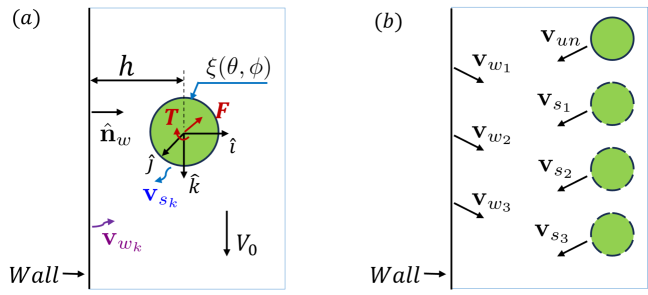
Figure 1: (a) Schematic of an elastic sphere translating parallel to a rigid wall at a specified velocity ($V_{0}\mathbf{\hat{k}}$), subjected to an external point force ($\mathbf{F}$) and a point torque ($\mathbf{T}$),

(b) unbounded velocity field ($\mathbf{v}_{un}$) undergoing subsequent reflections from wall (w) and sphere (s).

In this work, we use the method of reflections to analyse the wall effects on the dynamics of an elastic particle for two cases: first, when the gravity is aligned with particle velocity and second, when the gravity is in an arbitrary direction. The particle is considered as a weakly elastic sphere that translates parallel to a rigid wall. We model the particle using Navier elasticity equations and the fluid using the Stokes equations. An external point force and a point torque are applied to constrain the motion of the particle parallel to the wall as shown in figure 1(a). This setup corresponds to a resistance problem, in which the forces and the torques required to achieve a specified motion are determined. Murata solved the mobility problem for a weakly elastic sphere sedimenting under gravity in an unbounded domain (murata1980deformation, ). In a mobility problem, the motion of the particle is determined for a given set of forces and torques (kim2013microhydrodynamics, ). The results from the mobility problem can be used to derive those of the resistance problem for a rigid particle. However, such a relationship need not hold for a deformable particle. For a deformable particle, its shape depends on the force distribution acting on it, which can differ between the mobility and resistance problems. Murata’s results are for a specific force distribution that arises from the balance of gravity and hydrodynamic forces. However, the force distribution in our case is different, and therefore, we cannot use the results. We first analyse the motion of the particle in an unbounded domain as a resistance problem, and subsequently account for the wall effects using the method of reflections. We use a theoretical approach similar to the one used in Murata’s work, employing domain perturbation and series solutions for the governing equations of both the particle and fluid. The deformed shape we obtain for the first case differs from that obtained in Murata’s work, due to the difference in the force distribution in both problems. Further, Murata’s work uses Navier elasticity equations for modelling the particle while neglecting compressibility-induced density variations of the particle, whereas our work incorporates these effects. Our analysis of the unbounded problem in the second case reveals that hydrodynamic forces acting along the translational direction are modified by body forces acting perpendicular to the motion.The wall effects on particle dynamics are analyzed using the method of reflections. In the method, the disturbance velocity field generated by the particle’s motion in an unbounded domain is iteratively reflected between the wall and particle surfaces to satisfy boundary conditions on both. Reflections are carried out to obtain results up to $\textit{O}(1/H^{3})$ and $\textit{O}(1/H^{2})$ for the first and the second cases, respectively. Hydrodynamic forces due to wall effects generate a lift force away from the wall. We find that the point force balancing the lift is non-zero in the first case and zero in the second. Further, we find that the point torque is zero in the first case but non-zero in the second.

The subsequent sections of this manuscript are organized as follows: Section II presents the mathematical formulation, the governing equations, and the boundary conditions. The results are presented for the first and second case in section III.1 and III.2, respectively. The results for a neutrally buoyant particle and for zero gravity are presented in section III.1. We summarise our investigation in section IV.

II Mathematical formulation

We consider a weakly elastic spherical particle of undeformed radius ($R_{0}$) moving in a quiescent Newtonian fluid. The particle is translating parallel to a rigid wall at a velocity ($V_{0}\mathbf{\hat{k}}$) as shown in figure 1(a). The sphere centre is at a distance $h$ from the wall. An external point force ($\mathbf{F}$) and a point torque ($\mathbf{T}$) are applied at the centre to ensure that its motion is parallel to the wall. The unit vector normal to the wall ($\hat{\mathbf{n}}_{w}$) is aligned with the x-axis. We assume that the inertial effects in the flow are negligible compared to the viscous effects, i.e. the Reynolds number, defined as $Re=\rho_{f}V_{0}R_{0}/\mu\ll 1$. Here, $\rho_{f}$ and $\mu$ are the fluid density and viscosity, respectively. We assume that the fluid is incompressible and is governed by the Stokes equations given by

$$-\mathbf{\nabla}p+\mu\nabla^{2}\mathbf{v}+\rho_{f}\mathbf{g}={0},$$ (1)

$$\mathbf{\nabla}\cdot\mathbf{v}={0}.$$ (2)

In the above equations, $\mathbf{v}$ and $p$ are the velocity and pressure fields in the fluid, respectively, and $\mathbf{g}$ is the acceleration due to gravity. The particle is modelled using the Navier elasticity equations given by

$$\mathbf{[}\lambda+G]\mathbf{\nabla}\left(\mathbf{\nabla}\cdot\mathbf{u}\right)+G\mathbf{\nabla}^{2}\mathbf{u}+\rho_{p}\mathbf{g}+\mathbf{F}\delta(\mathbf{x})+\frac{1}{2}\left[\mathbf{\nabla}\delta(\mathbf{x})\times\mathbf{T}\right]={0}.$$ (3)

Above, $\mathbf{u}$ is the displacement field in the sphere, $\lambda$ and $G$ are the Lamé’s constants, and $\rho_{p}$ is the particle density. The fluid stress ($\boldsymbol{\sigma}$) is given by

$$\boldsymbol{\sigma}=-p\mathbf{I}+\mu\left(\nabla\mathbf{v}+[\nabla\mathbf{v}]^{T}\right),$$ (4)

and the solid stress ($\boldsymbol{\tau}$) is given by

$$\boldsymbol{\tau}=\lambda\left(\nabla\cdot\mathbf{u}\right)\mathbf{I}+G\left(\nabla\mathbf{u}+[\nabla\mathbf{u}]^{T}\right).$$ (5)

The variables in the problem are non-dimensionalised using the scalings given below

$$\mathbf{v^{*}}=\frac{\mathbf{v}}{V_{0}};p^{*}=\frac{pR_{0}}{\mu V_{0}};\boldsymbol{\sigma}^{*}=\frac{\boldsymbol{\sigma}R_{0}}{\mu V_{0}};\mathbf{u^{*}}=\frac{\mathbf{u}}{R_{0}};\boldsymbol{\tau}^{*}=\frac{\boldsymbol{\tau}}{G};H^{*}=\frac{h}{R_{0}}.$$ (6)

Non-dimensional variables are indicated using the asterisk symbol, which is omitted hereafter for brevity.

To analyse the dynamics of the particle, we express the solutions of (1) and (3) in a spherical coordinate system ($r$,$\theta$,$\phi$), whose origin coincides with the centre of the undeformed particle. The solutions are expressed in terms of $\xi$, $\theta$, and $\phi$, where $\xi$ is the non-dimensional radial coordinate defined by $\xi=r/R_{0}$, $\theta$ and $\phi$ are the polar and azimuthal angles, respectively. Since the wall-particle gap width is constant, the particle deforms and reaches a steady shape whose surface radius is defined by

$$\xi=1+f(\theta,\phi).$$ (7)

Here, $f$ quantifies the surface deformation and is a function of the polar and azimuthal angles. Note that in an unbounded domain, if gravity is aligned with the particle velocity, $f$ is axisymmetric about the translation axis (murata1980deformation, ). The function $f$ is related to the displacement field in the particle. The equation that relates the displacement of a material point on the deformed surface to its location on the undeformed surface is obtained in terms of $f$ as

$$1=\left[1+f-u_{r}|_{\xi=1+f(\theta,\phi)}\right]^{2}+\left[u_{\theta}|_{\xi=1+f(\theta,\phi)}\right]^{2}+\left[u_{\phi}|_{\xi=1+f(\theta,\phi)}\right]^{2}.$$ (8)

The deformability can be quantified using the ratio of the viscous to the elastic stresses defined as $\alpha=\mu V_{0}/(GR_{0})$. Since the particle is weakly deformable, elastic stresses dominate the viscous stresses ($\alpha\ll 1$) and the particle shape deviates slightly from the spherical shape. Noting that $\alpha$ is small, we have expanded all the variables in the problem as series in $\alpha$ and used the domain perturbation method (rangasbook, ; garyleal, ) to transfer the boundary conditions from the deformed to the undeformed surface of the particle. This generates the modified boundary conditions at the undeformed surface. The series solutions to the governing equations in (1)-(3) are used to find the fields that satisfy the modified boundary conditions. To include the effect of the wall, we have used the method of reflections (kim2013microhydrodynamics, ) and the fields at each order in $\alpha$ are expanded as series in $1/H$, the inverse of the non-dimensional wall-particle gap width. The external point force and the point torque are calculated based on the derived velocity and displacement fields at each order. We present the series solutions to the Stokes equations and the Navier elasticity equations in the above-mentioned spherical coordinate system in sections II.1 and II.2. We explain the domain perturbation method for the case of the particle translating in an unbounded domain in section II.3. The case of the particle translating parallel to a wall is discussed in section II.4. We summarise the steps to estimate the point force and the point torque in section II.5. The results are presented in section III.

II.1 Series solution to Stokes equations

The solutions to (1) and (2) are written in a general form (kim2013microhydrodynamics, ). The radial ($v_{r}$), tangential ($v_{\theta}$) and azimuthal ($v_{\phi}$) velocity components are given by

$$v_{r}=\sum_{n=1}^{\infty}\sum_{m=0}^{n} \left[\left(\frac{\xi^{-n}(n+1)}{2(2n-1)}P_{n}^{m}[A_{mn}\cos m\phi+\tilde{A}_{mn}\sin m\phi]\right)-\right.$$

$$\left.\vphantom{\frac{(n+1)}{2(2n-1)}}\left(\xi^{-n-2}(n+1)P_{n}^{m}[B_{mn}\cos m\phi+\tilde{B}_{mn}\sin m\phi]\right)\right],$$ (9)

$$v_{\theta}=\sum_{n=1}^{\infty}\sum_{m=0}^{n} \left[\left(\frac{\xi^{-n}(n-2)}{2n(2n-1)(2n+1)\sin\theta}\left[(n+1)(n+m)P_{n-1}^{m}-n(n-m+1)P_{n+1}^{m}\right]\right)\right.$$

$$\left.\left[A_{mn}\cos m\phi+\tilde{A}_{mn}\sin m\phi\right]-\right.$$

$$\left(\frac{\xi^{-n-2}}{(2n+1)\sin\theta}\left[(n+1)(n+m)P_{n-1}^{m}-n(n-m+1)P_{n+1}^{m}\right]\right)$$

$$\left.[B_{mn}\cos m\phi+\tilde{B}_{mn}\sin m\phi]+\right.$$

$$\left.\left(\frac{\xi^{-n-1}m}{\sin\theta}P_{n}^{m}[-V_{mn}\sin m\phi+\tilde{V}_{mn}\cos m\phi]\right)\right],$$ (10)

$$v_{\phi}=\sum_{n=1}^{\infty}\sum_{m=0}^{n} \left[\left(-\frac{\xi^{-n}(n-2)m}{2n(2n-1)\sin\theta}P_{n}^{m}[-A_{mn}\sin m\phi+\tilde{A}_{mn}\cos m\phi]\right)+\right.$$

$$\left.\left(\frac{\xi^{-n-2}m}{\sin\theta}P_{n}^{m}[-B_{mn}\sin m\phi+\tilde{B}_{mn}\cos m\phi]\right)+\right.$$

$$\left.\left(\frac{\xi^{-n-1}}{(2n+1)\sin\theta}\left[(n+1)(n+m)P_{n-1}^{m}-n(n-m+1)P_{n+1}^{m}\right]\right)\right.$$

$$\left.(V_{mn}\cos m\phi+\tilde{V}_{mn}\sin m\phi)\right],$$ (11)

respectively, and the pressure is given by

$$p =\xi\left[K_{fz}\cos\theta+K_{fx}\cos\phi\sin\theta+K_{fy}\sin\theta\sin\phi\right]$$

$$+\sum_{n=1}^{\infty}\sum_{m=0}^{n}\left[\xi^{-n-1}P_{n}^{m}(A_{mn}\cos m\phi+\tilde{A}_{mn}\sin m\phi)\right].$$ (12)

Here, $K_{fx}=\rho_{f}{R_{0}^{2}}g_{x}/(\mu V_{0})$, $K_{fy}=\rho_{f}{R_{0}^{2}}g_{y}/(\mu V_{0})$, $K_{fz}=\rho_{f}{R_{0}^{2}}g_{z}/(\mu V_{0})$, and $\mathbf{g}=g_{x}\mathbf{\hat{i}}+g_{y}\mathbf{\hat{j}}+g_{z}\mathbf{\hat{k}}$ in the Cartesian cordinate system. Above, $P^{m}_{n}$ denotes $P^{m}_{n}(\cos\theta)$, the associated Legendre polynomial of order $m$ and degree $n$. The constants, $A_{mn}$, $\tilde{A}_{mn}$, $B_{mn}$, $\tilde{B}_{mn}$, $V_{mn}$, and $\tilde{V}_{mn}$ are determined from the no-slip boundary conditions at the surface of the particle.

II.2 Series solution to Navier elasticity equations

The solution to (3) is expressed in a general form (kushch2013micromechanics, ). The radial ($u_{r}$), tangential ($u_{\theta}$) and azimuthal ($u_{\phi}$) displacement components are given by

$$u_{r}= \frac{1}{4\pi\xi}\left[F_{z}\cos\theta+F_{x}\cos\phi\sin\theta+F_{y}\sin\theta\sin\phi\right]-$$

$$\frac{2\lambda+7G}{30(\lambda+2G)}\xi^{2}\left[K_{pz}\cos\theta+K_{px}\cos\phi\sin\theta+K_{py}\sin\theta\sin\phi\right]\,+$$

$$\sum_{n=0}^{\infty}\sum_{m=0}^{n}\left[\xi^{n+1}P_{n}^{m}(B_{mn}^{1}\cos m\phi+B_{mn}^{0}\sin m\phi)\right]+\sum_{n=1}^{\infty}\sum_{m=0}^{n}\left[\xi^{n-1}P_{n}^{m}(C_{mn}^{1}\cos m\phi+C_{mn}^{0}\sin m\phi)\right],$$ (13)

$$u_{\theta}= \frac{(3G+\lambda)}{8\pi(2G+\lambda)\xi}\left(-F_{z}\sin\theta+\cos\theta\left[F_{x}\cos\phi+F_{y}\sin\phi\right]\right)+\frac{1}{8\pi\xi^{2}}\left(T_{y}\cos\phi-T_{x}\sin\phi\right)+$$

$$\frac{4\lambda+9G}{30(\lambda+2G)}\xi^{2}\left[K_{pz}\sin\theta-\cos\theta\left(K_{px}\cos\phi+K_{py}\sin\phi\right)\right]+$$

$$\frac{1}{\sin\theta}\left[\sum_{n=1}^{\infty}\sum_{m=0}^{n}\left(\frac{\xi^{n}m(2n+1)}{n(n+1)}P_{n}^{m}[-A_{mn}^{1}\sin m\phi+A_{mn}^{0}\cos m\phi]\right)\right]+$$

$$\frac{1}{\sin\theta}\left[\sum_{n=1}^{\infty}\sum_{m=0}^{n}\left(\frac{\xi^{n+1}[\lambda(n+3)+G(n+5)]}{(2n+1)(n+1)[\lambda\,n+G(n-2)]}\left[n(n-m+1)P_{n+1}^{m}-(n+1)(n+m)P_{n-1}^{m}\right]\right)\right.$$

$$\left.\vphantom{\sum_{m=0}^{n}\left(\xi^{n+1}\frac{n}{(2n+1)}\lambda_{Gf}\left[\frac{n-m+1}{n+1}P_{n+1}^{m}-\frac{n+m}{n}P_{n-1}^{m}\right]\right)}(B_{mn}^{1}\cos m\phi+B_{mn}^{0}\sin m\phi)\right]+$$

$$\frac{1}{\sin\theta}\left[\sum_{n=1}^{\infty}\sum_{m=0}^{n}\left(\frac{\xi^{n-1}}{(2n+1)n}\left[n(n-m+1)P_{n+1}^{m}-(n+1)(n+m)P_{n-1}^{m}\right]\right)\right.$$

$$\left.\vphantom{\sum_{m=0}^{n}\left(\xi^{n+1}\frac{n}{(2n+1)}\left[\frac{n-m+1}{n+1}P_{n+1}^{m}-\frac{n+m}{n}P_{n-1}^{m}\right]\right)}(C_{mn}^{1}\cos m\phi+C_{mn}^{0}\sin m\phi)\right]\text{\, and}$$ (14)

$$u_{\phi}= \frac{(3G+\lambda)}{8\pi(2G+\lambda)\xi}\left(F_{y}\cos\phi-F_{x}\sin\phi\right)-\frac{4\lambda+9G}{30(\lambda+2G)}\xi^{2}\left[K_{py}\cos\phi-K_{px}\sin\phi\right]+$$

$$\frac{1}{8\pi\xi^{2}}\left(T_{z}\sin\theta-\cos\theta\left[T_{x}\cos\phi+T_{y}\sin\phi\right]\right)+$$

$$\frac{1}{\sin\theta}\left[\left(\sum_{n=0}^{\infty}\sum_{m=0}^{n}\frac{-\xi^{n}}{(n+1)}\left[(n-m+1)P_{n+1}^{m}\right]+\sum_{n=1}^{\infty}\sum_{m=0}^{n}\frac{\xi^{n}}{n}\left[(n+m)P_{n-1}^{m}\right]\right)\right.$$

$$\left.\vphantom{\sum_{m=0}^{n}\xi^{n}\left(-\frac{(n-m+1)}{n+1}P_{n+1}^{m}+\frac{n+m}{n}P_{n-1}^{m}\right)}(A_{mn}^{1}\cos m\phi+A_{mn}^{0}\sin m\phi)\right]+$$

$$\frac{1}{\sin\theta}\left[\sum_{n=0}^{\infty}\sum_{m=0}^{n}\left(\frac{\xi^{n+1}m[\lambda(n+3)+G(n+5)]}{(n+1)[\lambda\,n+G(n-2)]}P_{n}^{m}[-B_{mn}^{1}\sin m\phi+B_{mn}^{0}\cos m\phi]\right)\right]+$$

$$\frac{1}{\sin\theta}\left[\sum_{n=1}^{\infty}\sum_{m=0}^{n}\left(\frac{\xi^{n-1}m}{n}P_{n}^{m}[-C_{mn}^{1}\sin m\phi+C_{mn}^{0}\cos m\phi]\right)\right].$$

respectively. Here, $K_{px}=\rho_{p}g_{x}R_{0}/G$, $K_{py}=\rho_{p}g_{y}R_{0}/G$, and $K_{pz}=\rho_{p}g_{z}R_{0}/G$. The constants, $A^{1}_{mn}$, $A^{0}_{mn}$, $B^{1}_{mn}$, $B^{0}_{mn}$, $C^{1}_{mn}$, and $C^{0}_{mn}$ are determined from the stress continuity at the particle surface. The displacement field for the point force and the point torque decays as $1/\xi$ and $1/\xi^{2}$, respectively as discussed in Appendix A. The Cartesian components of the force and torque are denoted by $F_{i}$ and $T_{i}$ ($i=x,y,z$), respectively. We have done the analysis in a particle-fixed coordinate system, and the point torque arrests the rotation of the particle. The constants that correspond to translation ($C^{1}_{10}$, $C^{1}_{11}$, and $C^{0}_{11}$) and rotation ($A^{1}_{10}$, $A^{1}_{11}$, and $A^{0}_{11}$) in the above series are, therefore, set to zero.

II.3 Domain pertubation method

In this section, we describe the domain perturbation method that is used to transfer the boundary conditions from the deformed surface of the particle to the undeformed surface as it translates in an unbounded domain. The particle deforms as it translates in the quiescent fluid. Since the particle is weakly deformable, the elastic stresses dominate the viscous stresses in the fluid $\left(\alpha=\mu V_{0}/(GR_{0})\ll 1\right)$. Therefore, the particle shape deviates slightly from the spherical shape. The deformation $f$ given in (7) has to be determined, as a part of the solution. The velocity boundary condition (no-slip) and the stress continuity on the deformed surface are given by

$$\mathbf{v}=0,$$ (16)

and

$$\boldsymbol{\tau}.\mathbf{\hat{n}}=\alpha\,\boldsymbol{\sigma}.\mathbf{\hat{n}},$$ (17)

respectively. Here, $\mathbf{\hat{n}}$ is the outward unit normal from the deformed surface defined by $\mathbf{\hat{n}}=\frac{\nabla S}{|\nabla S|}$, where $S=\xi-1-f(\theta,\phi)$. The stress boundary condition in terms of different stress components is given by

$$\tau_{rr}-\frac{\tau_{r\theta}}{\xi}\frac{\partial{f}}{\partial{\theta}}-\frac{\tau_{r\phi}}{\xi\sin\theta}\frac{\partial{f}}{\partial{\phi}}=\alpha\left[\sigma_{rr}-\frac{\sigma_{r\theta}}{\xi}\frac{\partial{f}}{\partial{\theta}}-\frac{\sigma_{r\phi}}{\xi\sin\theta}\frac{\partial{f}}{\partial{\phi}}\right],$$ (18)

$$\tau_{r\theta}-\frac{\tau_{\theta\theta}}{\xi}\frac{\partial{f}}{\partial{\theta}}-\frac{\tau_{\theta\phi}}{\xi\sin\theta}\frac{\partial{f}}{\partial{\phi}}=\alpha\left[\sigma_{r\theta}-\frac{\sigma_{\theta\theta}}{\xi}\frac{\partial{f}}{\partial{\theta}}-\frac{\sigma_{\theta\phi}}{\xi\sin\theta}\frac{\partial{f}}{\partial{\phi}}\right],$$ (19)

and

$$\tau_{r\phi}-\frac{\tau_{\theta\phi}}{\xi}\frac{\partial{f}}{\partial{\theta}}-\frac{\tau_{\phi\phi}}{\xi\sin\theta}\frac{\partial{f}}{\partial{\phi}}=\alpha\left[\sigma_{r\phi}-\frac{\sigma_{\theta\phi}}{\xi}\frac{\partial{f}}{\partial{\theta}}-\frac{\sigma_{\phi\phi}}{\xi\sin\theta}\frac{\partial{f}}{\partial{\phi}}\right].$$ (20)

Here, the $\tau_{ij}$ and $\sigma_{ij}$ with $i,j=r,\theta,\phi$ are the components of the solid and fluid stress tensor, respectively. The boundary conditions are shifted onto the undeformed surface using the domain perturbation method (garyleal, ). In this method, we first performed the Taylor series expansion of the boundary conditions (16)-(20) about $\xi=1$. The regular asymptotic expansion of the variables in the problem ($\mathbf{v}$, $\boldsymbol{\sigma}$, $p$, $\mathbf{u}$, $f$, $\boldsymbol{\tau}$, $\rho_{p}$, $\mathbf{F}$, $\mathbf{T}$) are then substituted into these expanded boundary conditions. The regular expansions of the variables as series in $\alpha$ are given by

$$\mathbf{v}=\mathbf{v}^{(0)}+\alpha\mathbf{v}^{(1)}+\alpha^{2}\mathbf{v}^{(2)}+...\,,$$ (21)

$$\boldsymbol{\sigma}=\boldsymbol{\sigma}^{(0)}+\alpha\boldsymbol{\sigma}^{(1)}+\alpha^{2}\boldsymbol{\sigma}^{(2)}+...\,,$$ (22)

$$p=p^{(0)}+\alpha p^{(1)}+\alpha^{2}p^{(2)}+...\,,$$ (23)

$$\mathbf{u}=\alpha\mathbf{u}^{(1)}+\alpha^{2}\mathbf{u}^{(2)}+...\,,$$ (24)

$$f=\alpha f^{(1)}+\alpha^{2}f^{(2)}+...\,,$$ (25)

$$\boldsymbol{\tau}=\alpha\boldsymbol{\tau}^{(1)}+\alpha^{2}\boldsymbol{\tau}^{(2)}+...\,,$$ (26)

$$\rho_{p}=\rho_{p}^{(0)}+\alpha\rho_{p}^{(1)}+\alpha^{2}\rho_{p}^{(2)}+...\,,$$ (27)

$$\mathbf{F}=\mathbf{F}^{(0)}+\alpha\mathbf{F}^{(1)}+\alpha^{2}\mathbf{F}^{(2)}+...\,,$$ (28)

and

$$\mathbf{T}=\mathbf{T}^{(0)}+\alpha\mathbf{T}^{(1)}+\alpha^{2}\mathbf{T}^{(2)}+...\,.$$ (29)

Note that the leading-order term in the series for the displacement field (24), the deformation (25), and the solid stress (26) arising from the deformation are O($\alpha$).

II.3.1 Modified velocity boundary condition on the undeformed surface ($\xi=1$)

We have performed Taylor expansion of (16) about the undeformed surface ($\xi=1$) and substituted the velocity and deformation expansions from (21) and (25), respectively, to obtain the modified velocity boundary conditions at various orders in $\alpha$. At leading-order, the boundary conditions are given by

$$\mathbf{v}^{(0)} =0\,\,\mbox{as $\xi$ =1},$$

$$\rightarrow-1\mathbf{\hat{k}}\,\,\mbox{as $\xi\rightarrow\infty$}.$$ (30)

At O($\alpha$), it is

$$\mathbf{v}^{(1)}+f^{(1)}\frac{\partial{\mathbf{v}^{(0)}}}{\partial{\xi}}=0,$$ (31)

and at O($\alpha^{2}$), it is

$$\mathbf{v}^{(2)}+f^{(1)}\frac{\partial{\mathbf{v}^{(1)}}}{\partial{\xi}}+f^{(2)}\frac{\partial{\mathbf{v}^{(0)}}}{\partial{\xi}}+\frac{\left[f^{(1)}\right]^{2}}{2}\frac{\partial^{2}{\mathbf{v}^{(0)}}}{\partial{\xi}^{2}}=0.$$ (32)

Further, the velocity fields $\mathbf{v}^{(1)}$ and $\mathbf{v}^{(2)}$ decays as $\xi\rightarrow\infty$. Note that the boundary conditions in (31) and (32) are nonlinear. Although the governing equations are linear, the nonlinearity arises from applying the boundary conditions at the deformed surface whose shape is a part of the solution.

II.3.2 Modified stress boundary conditions on the undeformed surface ($\xi=1$)

We have performed Taylor expansion of (17) about the undeformed surface ($\xi=1$) and substituted the fluid stress, deformation, and solid stress expansions from (22), (25), and (26), respectively, to obtain the modified stress boundary conditions at various orders in $\alpha$.
At O($\alpha$), the stress boundary conditions are

$$\tau^{(1)}_{rr}=\sigma^{(0)}_{rr},$$ (33)

$$\tau^{(1)}_{r\theta}=\sigma^{(0)}_{r\theta},$$ (34)

$$\tau^{(1)}_{r\phi}=\sigma^{(0)}_{r\phi}.$$ (35)

At O($\alpha^{2}$), they are

$$\tau_{rr}^{(2)}=\sigma_{rr}^{(1)}+f^{(1)}\frac{\partial}{\partial{\xi}}\left[\sigma_{rr}^{(0)}-\tau_{rr}^{(1)}\right],$$ (36)

$$\tau_{r\theta}^{(2)}=\sigma_{r\theta}^{(1)}-f^{(1)}\frac{\partial}{\partial{\xi}}\left[\tau_{r\theta}^{(1)}-\sigma_{r\theta}^{(0)}\right]+\frac{\partial{f^{(1)}}}{\partial{\theta}}\left[\tau_{\theta\theta}^{(1)}-\sigma_{\theta\theta}^{(0)}\right]+\frac{1}{\sin\theta}\frac{\partial{f^{(1)}}}{\partial{\phi}}\left[\tau_{\theta\phi}^{(1)}-\sigma_{\theta\phi}^{(0)}\right],$$ (37)

$$\tau_{r\phi}^{(2)}=\sigma_{r\phi}^{(1)}-f^{(1)}\frac{\partial}{\partial{\xi}}\left[\tau_{r\phi}^{(1)}-\sigma_{r\phi}^{(0)}\right]+\frac{\partial{f^{(1)}}}{\partial{\theta}}\left[\tau_{\theta\phi}^{(1)}-\sigma_{\theta\phi}^{(0)}\right]+\frac{1}{\sin\theta}\frac{\partial{f^{(1)}}}{\partial{\phi}}\left[\tau_{\phi\phi}^{(1)}-\sigma_{\phi\phi}^{(0)}\right],$$ (38)

and at O($\alpha^{3}$), they are

$$\tau_{rr}^{(3)}= \sigma_{rr}^{(2)}-f^{(1)}\frac{\partial}{\partial{\xi}}\left[\tau_{rr}^{(2)}-\sigma_{rr}^{(1)}\right]-f^{(2)}\frac{\partial}{\partial{\xi}}\left[\tau_{rr}^{(1)}-\sigma_{rr}^{(0)}\right]-\frac{\left[f^{(1)}\right]^{2}}{2}\frac{\partial^{2}}{\partial{\xi}^{2}}\left[\tau_{rr}^{(1)}-\sigma_{rr}^{(0)}\right]+$$

$$\frac{\partial f^{(2)}}{\partial{\theta}}\left[\tau_{r\theta}^{(1)}-\sigma_{r\theta}^{(0)}\right]+\frac{\partial f^{(1)}}{\partial{\theta}}\left[\tau_{r\theta}^{(2)}-\sigma_{r\theta}^{(1)}\right]+f^{(1)}\frac{\partial f^{(1)}}{\partial{\theta}}\frac{\partial}{\partial{\xi}}\left[\tau_{r\theta}^{(1)}-\sigma_{r\theta}^{(0)}\right]+$$

$$\frac{1}{\sin\theta}\left(\frac{\partial f^{(2)}}{\partial{\phi}}\left[\tau_{r\phi}^{(1)}-\sigma_{r\phi}^{(0)}\right]+\frac{\partial f^{(1)}}{\partial{\phi}}\left[\tau_{r\phi}^{(2)}-\sigma_{r\phi}^{(1)}\right]+f^{(1)}\frac{\partial f^{(1)}}{\partial{\phi}}\frac{\partial}{\partial{\xi}}\left[\tau_{r\phi}^{(1)}-\sigma_{r\phi}^{(0)}\right]\right)-$$

$$f^{(1)}\frac{\partial f^{(1)}}{\partial{\theta}}\left[\tau_{r\theta}^{(1)}-\sigma_{r\theta}^{(0)}\right]-\frac{1}{\sin\theta}\left(f^{(1)}\frac{\partial f^{(1)}}{\partial{\phi}}\left[\tau_{r\phi}^{(1)}-\sigma_{r\phi}^{(0)}\right]\right),$$ (39)

$$\tau_{r\theta}^{(3)}= \sigma_{r\theta}^{(2)}-f^{(1)}\frac{\partial}{\partial{\xi}}\left[\tau_{r\theta}^{(2)}-\sigma_{r\theta}^{(1)}\right]-f^{(2)}\frac{\partial}{\partial{\xi}}\left[\tau_{r\theta}^{(1)}-\sigma_{r\theta}^{(0)}\right]-\frac{\left[f^{(1)}\right]^{2}}{2}\frac{\partial^{2}}{\partial{\xi}^{2}}\left[\tau_{r\theta}^{(1)}-\sigma_{r\theta}^{(0)}\right]+$$

$$\frac{\partial f^{(2)}}{\partial{\theta}}\left[\tau_{\theta\theta}^{(1)}-\sigma_{\theta\theta}^{(0)}\right]+\frac{\partial f^{(1)}}{\partial{\theta}}\left[\tau_{\theta\theta}^{(2)}-\sigma_{\theta\theta}^{(1)}\right]+f^{(1)}\frac{\partial f^{(1)}}{\partial{\theta}}\frac{\partial}{\partial{\xi}}\left[\tau_{\theta\theta}^{(1)}-\sigma_{\theta\theta}^{(0)}\right]+$$

$$\frac{1}{\sin\theta}\left(\frac{\partial f^{(2)}}{\partial{\phi}}\left[\tau_{\theta\phi}^{(1)}-\sigma_{\theta\phi}^{(0)}\right]+\frac{\partial f^{(1)}}{\partial{\phi}}\left[\tau_{\theta\phi}^{(2)}-\sigma_{\theta\phi}^{(1)}\right]+f^{(1)}\frac{\partial f^{(1)}}{\partial{\phi}}\frac{\partial}{\partial{\xi}}\left[\tau_{\theta\phi}^{(1)}-\sigma_{\theta\phi}^{(0)}\right]\right)-$$

$$f^{(1)}\frac{\partial f^{(1)}}{\partial{\theta}}\left[\tau_{\theta\theta}^{(1)}-\sigma_{\theta\theta}^{(0)}\right]-\frac{1}{\sin\theta}\left(f^{(1)}\frac{\partial f^{(1)}}{\partial{\phi}}\left[\tau_{\theta\phi}^{(1)}-\sigma_{\theta\phi}^{(0)}\right]\right),$$ (40)

$$\tau_{r\phi}^{(3)}= \sigma_{r\phi}^{(2)}-f^{(1)}\frac{\partial}{\partial{\xi}}\left[\tau_{r\phi}^{(2)}-\sigma_{r\phi}^{(1)}\right]-f^{(2)}\frac{\partial}{\partial{\xi}}\left[\tau_{r\phi}^{(1)}-\sigma_{r\phi}^{(0)}\right]-\frac{\left[f^{(1)}\right]^{2}}{2}\frac{\partial^{2}}{\partial{\xi}^{2}}\left[\tau_{r\phi}^{(1)}-\sigma_{r\phi}^{(0)}\right]+$$

$$\frac{\partial f^{(2)}}{\partial{\theta}}\left[\tau_{\theta\phi}^{(1)}-\sigma_{\theta\phi}^{(0)}\right]+\frac{\partial f^{(1)}}{\partial{\theta}}\left[\tau_{\theta\phi}^{(2)}-\sigma_{\theta\phi}^{(1)}\right]+f^{(1)}\frac{\partial f^{(1)}}{\partial{\theta}}\frac{\partial}{\partial{\xi}}\left[\tau_{\theta\phi}^{(1)}-\sigma_{\theta\phi}^{(0)}\right]+$$

$$\frac{1}{\sin\theta}\left(\frac{\partial f^{(2)}}{\partial{\phi}}\left[\tau_{\phi\phi}^{(1)}-\sigma_{\phi\phi}^{(0)}\right]+\frac{\partial f^{(1)}}{\partial{\phi}}\left[\tau_{\phi\phi}^{(2)}-\sigma_{\phi\phi}^{(1)}\right]+f^{(1)}\frac{\partial f^{(1)}}{\partial{\phi}}\frac{\partial}{\partial{\xi}}\left[\tau_{\phi\phi}^{(1)}-\sigma_{\phi\phi}^{(0)}\right]\right)-$$

$$f^{(1)}\frac{\partial f^{(1)}}{\partial{\theta}}\left[\tau_{\theta\phi}^{(1)}-\sigma_{\theta\phi}^{(0)}\right]-\frac{1}{\sin\theta}\left(f^{(1)}\frac{\partial f^{(1)}}{\partial{\phi}}\left[\tau_{\phi\phi}^{(1)}-\sigma_{\phi\phi}^{(0)}\right]\right).$$ (41)

The deformation of the surface at different orders $f^{(1)}$ and $f^{(2)}$ appearing in the modified boundary conditions are obtained by expanding (8) using Taylor series about $\xi=1$ and substituting (24) and (25). At O($\alpha$), $f^{(1)}$ is given by

$$f^{(1)}=\left.u_{r}^{(1)}\right|_{\xi=1}.$$ (42)

At O($\alpha^{2}$), $f^{(2)}$ is given by

$$f^{(2)}=\left(u_{r}^{(2)}+f^{(1)}\frac{\partial{u_{r}^{(1)}}}{\partial{\xi}}-\frac{\left[u_{\theta}^{(1)}\right]^{2}+\left[u_{\phi}^{(1)}\right]^{2}}{2}\right)\left.\vphantom{\frac{\left[u_{\theta}^{(1)}\right]^{2}}{2}}\right|_{\xi=1}.$$ (43)

The modified boundary conditions, together with the series solutions described in the previous sections, are used to calculate all the variables defined in (21)-(29) in the unbounded domain.

II.4 Method of reflections

To capture the effect of the wall on the dynamics of the translating particle, we have employed the method of reflections (kim2013microhydrodynamics, ). The unbounded velocity field ($\mathbf{v}_{un}$) doesn’t satisfy the no-slip boundary condition at the wall (see figure 1(b)). The velocity field is alternatively reflected from the wall ($\mathbf{v}_{w_{k}}$) and the sphere ($\mathbf{v}_{s_{k}}$), and the reflected fields are added to the unbounded velocity field, to satisfy the boundary conditions at both the surfaces to the desired accuracy. The desired accuracy can be quantified in algebraic powers of $1/H$. Therefore, the reflected velocity fields are expanded as series in $1/H$. The total velocity field at each order in $\alpha^{n}$ ($n=0,1,2..$) is written as

$$\mathbf{v}^{(n)}=\mathbf{v}^{(n)}_{un}+ \frac{{\mathbf{v}}^{(n,\scalebox{0.6}{$H$})}_{w_{1}}}{H}+\frac{{\mathbf{v}}^{(n,\scalebox{0.6}{$H^{2}$})}_{w_{1}}}{H^{2}}+...+\frac{\mathbf{v}^{(n,\scalebox{0.6}{$H$})}_{s_{1}}}{H}+\frac{\mathbf{v}^{(n,\scalebox{0.6}{$H^{2}$})}_{w_{2}}}{H^{2}}+\frac{\mathbf{v}^{(n,\scalebox{0.6}{$H^{3}$})}_{w_{2}}}{H^{3}}+...+\frac{\mathbf{v}^{(n,\scalebox{0.6}{$H^{2}$})}_{s_{2}}}{H^{2}}+$$

$$\frac{\mathbf{v}^{(n,\scalebox{0.6}{$H^{3}$})}_{w_{3}}}{H^{3}}+\frac{\mathbf{v}^{(n,\scalebox{0.6}{$H^{4}$})}_{w_{3}}}{H^{4}}+...+\frac{\mathbf{v}^{(n,\scalebox{0.6}{$H^{3}$})}_{s_{3}}}{H^{3}}+\frac{\mathbf{v}^{(n,\scalebox{0.6}{$H^{4}$})}_{w_{4}}}{H^{4}}+...\,.$$ (44)

Here, the subscripts $()_{un}$ and $()_{w_{k}}$ denote the unbounded field and the $k^{th}$ reflected field from the wall, respectively. The subscript $()_{s_{k}}$ indicates that the velocity field includes the effect of $k^{th}$ reflection from the sphere. The superscript $(n,H^{p})$ indicates $1/H^{p}$ term in the series at O($\alpha^{n}$). Similar to the velocity field, the fluid stress $\boldsymbol{\sigma}^{(n)}$ and pressure $p^{(n)}$ are also expanded as series in $1/H$. The displacement $\mathbf{u}^{(n)}$ at each order in $\alpha^{n}(n=1,2,...)$ is expanded as a series in $1/H$ as

$$\mathbf{u}^{(n)}=\mathbf{u}^{(n)}_{un}+\frac{\mathbf{u}^{(n,\scalebox{0.6}{$H$})}_{s_{1}}}{H}+\frac{\mathbf{u}^{(n,\scalebox{0.6}{$H^{2}$})}_{s_{2}}}{H^{2}}+\frac{\mathbf{u}^{(n,\scalebox{0.6}{$H^{3}$})}_{s_{3}}}{H^{3}}+...\,.$$ (45)

Similar to the displacement field, the solid stress $\boldsymbol{\tau}^{(n)}$, deformation $f^{(n)}$, point force $\mathbf{F}^{(n)}$ and point torque $\mathbf{T}^{(n)}$ are expanded as series in $1/H$. We have derived the results till O($1/H^{3}$), which needs three reflections from the wall in the first case where gravity is aligned with the particle velocity. In the second case where gravity is in an arbitrary direction, the results are derived till O($1/H^{2}$), which needs two reflections from the wall.

II.5 Solution procedure

Below, we describe the steps involved in calculating the point force and the point torque required to make the particle translate parallel to the wall. Steps (i)-(iv) are for an unbounded domain, and (v)-(ix) are for capturing the wall effects using the method of reflections.

2. First, we calculated the fields ($\mathbf{v}^{(0)}_{un},p^{(0)}_{un}$) surrounding the particle in an unbounded domain. At O(1), the constants in (9)-(11) are determined by applying the velocity boundary condition in (30) and the corresponding fluid stress field $\boldsymbol{\sigma}_{un}^{(0)}$ is calculated.

4. Using stress continuity in (33)-(35), $\boldsymbol{\tau}_{un}^{(1)}$, $\mathbf{u}_{un}^{(1)}$, $\mathbf{F}_{un}^{(0)}$, $\mathbf{T}_{un}^{(0)}$, and $f_{un}^{(1)}$ are calculated.

6. We then used (31) to determine $\mathbf{v}_{un}^{(1)}$ and in turn calculate $\boldsymbol{\sigma}_{un}^{(1)}$.

8. Above steps (ii and iii) are repeated at the next orders in $\alpha$ to determine the velocity and the stress fields in the fluid, the external forces and the external torques till O($\alpha^{2}$), and the displacement and stress fields in the solid till O($\alpha^{3}$).

10. To capture the wall effects, the unbounded velocity and pressure fields till O($\alpha^{2}$) are reflected from the wall, to determine the first wall reflected fields at various orders given by $\left[\frac{\mathbf{v}^{(0,\scalebox{0.6}{$H$})}_{w_{1}}}{H}+\alpha\frac{\mathbf{v}^{(1,\scalebox{0.6}{$H$})}_{w_{1}}}{H}+\alpha^{2}\frac{\mathbf{v}^{(2,\scalebox{0.6}{$H$})}_{w_{1}}}{H}\right]$, $\left[\frac{\mathbf{v}^{(0,\scalebox{0.6}{$H^{2}$})}_{w_{1}}}{H^{2}}+\alpha\frac{\mathbf{v}^{(1,\scalebox{0.6}{$H^{2}$})}_{w_{1}}}{H^{2}}\right]$, and $\frac{{\mathbf{v}}^{(0,\scalebox{0.6}{$H^{3}$})}_{w_{1}}}{H^{3}}$.

12. The velocity fields ${\mathbf{v}}^{(n,\scalebox{0.6}{$H$})}_{w_{1}}$(with n=0,1,2) are reflected from the sphere to determine the first sphere reflected fields given by $\left[\frac{\mathbf{v}^{(0,\scalebox{0.6}{$H$})}_{s_{1}}}{H}+\alpha\frac{\mathbf{v}^{(1,\scalebox{0.6}{$H$})}_{s_{1}}}{H}+\alpha^{2}\frac{\mathbf{v}^{(2,\scalebox{0.6}{$H$})}_{s_{1}}}{H}\right]$ and the displacement fields given by $\left[\alpha\frac{\mathbf{u}^{(1,\scalebox{0.6}{$H$})}_{s_{1}}}{H}+\alpha^{2}\frac{\mathbf{u}^{(2,\scalebox{0.6}{$H$})}_{s_{1}}}{H}\right]$ using the boundary conditions at the sphere surface. We followed the same steps as those described for the unbounded domain to calculate the higher-order term in $\alpha$.

14. The velocity fields ${\mathbf{v}}^{(n,\scalebox{0.6}{$H$})}_{s_{1}}$ (with n=0,1) are reflected from the wall to determine the second wall reflected fields given by $\left[\frac{\mathbf{v}^{(0,\scalebox{0.6}{$H^{2}$})}_{w_{2}}}{H^{2}}+\alpha\frac{\mathbf{v}^{(1,\scalebox{0.6}{$H^{2}$})}_{w_{2}}}{H^{2}}\right]$ and $\frac{\mathbf{v}^{(0,\scalebox{0.6}{$H^{3}$})}_{w_{2}}}{H^{3}}$. All the O($1/H^{2}$) terms from the first and second wall reflections are used to determine the second sphere reflected fields given by $\left[\frac{\mathbf{v}^{(0,\scalebox{0.6}{$H^{2}$})}_{s_{2}}}{H^{2}}+\alpha\frac{\mathbf{v}^{(1,\scalebox{0.6}{$H^{2}$})}_{s_{2}}}{H^{2}}\right]$ and the displacement field given by $\left[\alpha\frac{\mathbf{u}^{(1,\scalebox{0.6}{$H^{2}$})}_{s_{2}}}{H^{2}}\right]$ using the boundary conditions at the sphere surface.

16. The velocity field ${\mathbf{v}}^{(0,\scalebox{0.6}{$H^{2}$})}_{s_{2}}$ is reflected from the wall to determine the third wall reflected field given by $\frac{{\mathbf{v}}^{(0,\scalebox{0.6}{$H^{3}$})}_{w_{3}}}{H^{3}}$. All the O($1/H^{3}$) terms in the first three wall reflections are used to calculate the third sphere reflected field given by $\frac{{\mathbf{v}}^{(0,\scalebox{0.6}{$H^{3}$})}_{s_{3}}}{H^{3}}$.

18. At each of the reflections from the sphere, we also determine the point force and the point torque at different orders.

III Results

Below, we discuss the results of our analysis. The discussion is presented for two cases: 1) gravity aligned with the particle velocity in section III.1 and 2) gravity in an arbitrary direction in section III.2.

III.1 Gravity aligned with particle velocity

First, we discuss the results for the case of translation of the particle along the direction of gravity ($\mathbf{g}=g_{z}\mathbf{\hat{k}}$) in an unbounded domain. The leading-order velocity field [$\mathbf{v}_{un}^{(0)}$] is obtained by applying (30) to determine the constants in the series solution in section II.1. The field is the same as that in a uniform flow past a rigid sphere of radius $R_{0}$ in an unbounded domain (guazzelli2011physical, ). The stress field at O($\alpha$) in the solid is calculated using the boundary conditions (33)-(35), and the corresponding displacement components are obtained as

$${u^{(1)}_{un,r}}=\frac{1}{\xi}C_{1}\cos\theta+\xi^{2}C_{2}\cos\theta,$$ (46)

$$u^{(1)}_{un,\theta}=\frac{1}{\xi}\left[-\frac{3+\gamma}{4+2\gamma}C_{1}\right]\sin\theta+\xi^{2}\left[\frac{(3+2\gamma)(2K_{fz}-9(1+\gamma))-K_{fz}\gamma\tilde{\rho}}{(-1+\gamma)(9-2K_{fz}+9\gamma)+K_{fz}(4+5\gamma)\tilde{\rho}}C_{2}\right]\sin\theta.$$ (47)

Here,

$$C_{1}=\frac{1}{6}\left(9-2K_{fz}(-1+\tilde{\rho})\right),$$

$$C_{2}=-\frac{-9+9\gamma^{2}+K_{fz}(2+4\tilde{\rho}+\gamma(-2+5\tilde{\rho}))}{6(2+\gamma)(2+3\gamma)},$$ (48)

Above, $\tilde{\rho}=\rho^{(0)}_{p}/\rho_{f}$ and $K_{fz}=\rho_{f}{R_{0}^{2}}g_{z}/(\mu V_{0})$, ratio of gravitational to the viscous forces. Further, $\gamma$ is the ratio of the bulk modulus ($\lambda$) to the shear modulus ($G$). The surface deformation $f^{(1)}_{un}$ is calculated from (42) and is obtained as

$$f^{(1)}_{un}=C_{3}\cos\theta,$$ (49)

where $C_{3}=C_{1}+C_{2}$. Using the boundary condition (31), the velocity components and pressure in the fluid at O($\alpha$) are obtained as

$$v^{(1)}_{un,r}=\left[\frac{1}{\xi^{2}}-\frac{1}{\xi^{4}}\right]\frac{3\,C_{3}}{4}(3\cos^{2}\theta-1),$$ (50)

$$v^{(1)}_{un,\theta}=-\frac{1}{\xi^{4}}\left[\frac{3\,C_{3}}{2}\right]\cos\theta\sin\theta,$$ (51)

$$v^{(1)}_{un,\phi}=0,$$ (52)

$$p^{(1)}_{un}=\frac{1}{\xi^{3}}\left[\frac{3\,C_{3}}{2}\right](3\cos^{2}\theta-1).$$ (53)

The stress field in the solid at O($\alpha^{2}$) is calculated using the boundary conditions (36)-(38) and the corresponding displacement components are obtained as

$$u^{(2)}_{un,r}=\xi\left[A_{1}+A_{2}\cos^{2}\theta\right]+\xi^{3}A_{3}(1-3\cos^{2}\theta),$$ (54)

$$u^{(2)}_{un,\theta}=-\xi A_{2}\cos\theta\sin\theta+\xi^{3}\left[\frac{(7+5\gamma)}{\gamma}A_{3}\right]\sin\theta\cos\theta.$$ (55)

Here,

$$A_{1}=\left[\frac{-168+\gamma(-48+3\gamma(152+97\gamma)-2K_{fz}(48+\gamma(98+45\gamma))(-1+\tilde{\rho}))}{4(2+\gamma)(2+3\gamma)(14+19\gamma)}\right]C_{3},$$

$$A_{2}=\left[\frac{-336-3\gamma(214+97\gamma)+2K_{fz}(4+5\gamma)(14+9\gamma)(-1+\tilde{\rho})}{4(2+\gamma)(14+19\gamma)}\right]C_{3},$$

$$A_{3}=\left[\frac{2\gamma(1+\gamma)(-9+2K_{fz}(-1+\tilde{\rho}))}{(2+\gamma)(14+19\gamma)}\right]C_{3}.$$ (56)

The surface deformation $f^{(2)}_{un}$ is calculated from (43) and is obtained as

$$f^{(2)}_{un}=D_{1}+D_{2}\cos^{2}\theta-\frac{1}{2}D_{3}^{2}\sin^{2}\theta.$$ (57)

Here,

$$D_{1}=A_{1}+A_{3},$$

$$D_{2}=A_{2}-3A_{3}-C_{3}(-3C_{2}+C_{3}),$$

$$D_{3}=\frac{(C_{2}-C_{3})(3+\gamma)}{2(2+\gamma)}+\frac{C_{2}\left((3+2\gamma)(2K_{fz}-9(1+\gamma))-K_{fz}\gamma\tilde{\rho}\right)}{(-1+\gamma)(9-2K_{fz}+9\gamma)+K_{fz}(4+5\gamma)\tilde{\rho}}.$$ (58)

Using (32), we calculated $\mathbf{v}^{(2)}_{un}$ and then derived the stress field $\boldsymbol{\tau}^{(3)}_{un}$ using the boundary conditions (39)-(41). The expressions for components of $\mathbf{v}^{(2)}_{un}$ are provided in (78) and (79) of Appendix B. The point force till O($\alpha^{2}$) in dimensional form is obtained as

$$\mathbf{F}_{un} =6\pi\mu V_{0}R_{0}\left(\left[1+\frac{2K_{fz}}{9}\left(1-\tilde{\rho}\right)\right]+\alpha^{2}\left[\vphantom{\frac{2K_{fz}}{9}}E_{1}+K_{fz}^{3}(E_{2}I_{1})+K_{fz}^{2}(E_{2}E_{3}I_{2})+\right.\right.$$

$$\left.\left.K_{fz}(E_{4}E_{2}I_{3})\vphantom{\frac{2K_{fz}}{9}}\right]\right)\mathbf{\hat{k}}\,.$$ (59)

The expressions for $E_{1}$, $E_{2}$, $E_{3}$, $E_{4}$, $I_{1}$, $I_{2}$, and $I_{3}$ in the equation are given in (80)-(84) of Appendix B. The leading order force in the equation reduces to the sum of Stokes drag and the buoyancy force on a rigid sphere. The particle should not experience a hydrodynamic lift force or a torque due to the symmetry of the flow field about the $z$-axis in the unbounded domain. Consistently, the point force at O($\alpha^{2}$) in the equation acts only along gravity ($z$-axis) and the point torque is also zero. The point force at O($\alpha^{2}$) balances the hydrodynamic forces arising from the change in the particle shape and the buoyancy force. The change in the buoyancy force at O($\alpha^{2}$) arises from compressibility-induced variations in the particle’s volume and density.

To analyse the shape of the deformed particle, we have plotted it on $y=0$ plane as shown in figure 2(a).

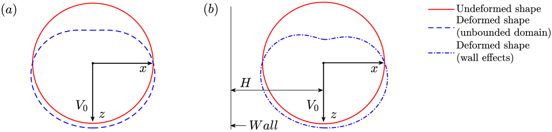
Figure 2: The shape of the deformed sphere on $xz$ plane at $\alpha=0.2$, $\tilde{\rho}=1.05$, $K_{fz}=0.5$ and $\gamma=2$ in the (a) unbounded domain and (b) in the presence of wall at $H=2.5$.

As is evident in the figure, the shape is symmetric about the $z$-axis. The dip at the top is due to the effect of the point force applied at the centre of the particle. The shape that we obtain differs from that obtained by an earlier work(murata1980deformation, ). Murata calculated the velocity of a weakly elastic spherical particle sedimenting due to gravity. He showed that the particle deforms to a prolate spheroid at O($\alpha^{2}$). The shape difference between ours and Murata’s work arises from the varying force distributions: our problem considers equilibrium between external, gravitational, and hydrodynamic forces, whereas Murata’s formulation considers only gravitational and hydrodynamic forces. Consequently, the hydrodynamic forces acting on the particle differ between the two problems. Additionally, our approach accounts for the density change due to the compressibility of the particle, an aspect not considered in Murata’s calculation, although he models the particle as a compressible one.

The deformed shape of the particle depends on the ratio of the particle density to the ambient fluid ($\tilde{\rho}$). For a particle heavier than the surrounding fluid, as $K_{fz}$ increases, the external force required to balance hydrodynamic drag diminishes, resulting in a reduction in the dip in the particle’s upper section as shown in figure 3(a). Conversely, for a particle lighter than the ambient fluid, an increase in $K_{fz}$ necessitates a larger external force to sustain translation, which in turn enhances the dip in the particle’s upper section as shown in figure 3(b).

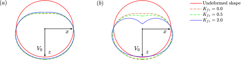
Figure 3: Variation in the shape of the deformed sphere in the unbounded domain as a function of $K_{fz}$ at $\gamma=2$, $\alpha=0.2$ when (a) the particle is denser than fluid, $\tilde{\rho}=1.05$ and (b) when the particle is lighter than the fluid, $\tilde{\rho}=0.05$.

Figure 4(a) illustrates the variation of the maximum principal stress (based on its absolute value) along the surface of a heavier particle for $K_{fz}=0.5$. In figure 4(b), the stress is plotted against $\theta$ for different values of $K_{fz}$. The maximum principal stress is tensile in nature near $\theta=\pi$, the location of the dip in the deformed shape, due to the point force. As $K_{fz}$ increases, the point force diminishes, leading to a reduction in the maximum principal stress near $\theta=\pi$. This trend aligns with the less pronounced dip seen in figure 3(a).

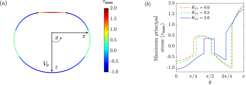
Figure 4: Variation of the maximum principal stress (based on its absolute value) along the particle surface in the unbounded domain at $\gamma=2$, $\alpha=0.2$, $\tilde{\rho}=1.05$ (a) for $K_{fz}=0.5$ and (b) for different values of $K_{fz}$, plotted for $\theta$ from $0$ to $\pi$.

Now we discuss the case of the particle translating next to a wall. In the presence of the wall, the calculations are carried out using the method of reflections described in section II.4. The velocity and displacement fields are calculated at orders $1/H$, $\alpha/H$, $\alpha^{2}/H$, $1/H^{2}$, $\alpha/H^{2}$, and $1/H^{3}$. The surface deformation till the order considered is obtained as

$$f =f_{un}+\alpha\left[\frac{B_{1}\cos\theta}{H}\left(1+\frac{9}{16H}\right)+\frac{45\cos\phi\sin 2\theta}{64H^{2}}\right]+\alpha^{2}\left[\left(\frac{B_{2}}{H}+K_{fz}\frac{B_{3}}{H}\right)+\right.$$

$$\left.\left(\frac{B_{4}}{H}+K_{fz}\frac{B_{5}}{H}\right)\cos 2\theta\right].$$ (60)

The expressions for $B_{1}$, $B_{2}$, $B_{3}$, $B_{4}$, and $B_{5}$ in the equation are given in (87)-(90) of Appendix B. The deformation in the unbounded domain $f_{un}=\alpha f^{(1)}_{un}+\alpha^{2}f^{(2)}_{un}$, where $f^{(1)}_{un}$ and $f^{(2)}_{un}$ are presented in (49) and (57), respectively. Due to the presence of the wall, the deformed shape is not symmetric about the $z$-axis and is a function of $\phi$ at O($\alpha/H^{2}$). This contrasts with the unbounded case, where the deformed shape remains independent of $\phi$. We have plotted the shape of the particle in the $xz$ plane passing through the origin in figure 2(b) to illustrate the asymmetry. The dash-dot curve is plotted using (7) and the shape is not symmetric about the $z$-axis.

The point force on the particle till the order considered is obtained as

$$\mathbf{F} =\mathbf{F_{un}}+6\pi\mu V_{0}R_{0}\left(\left[\frac{9}{16H}+\frac{81}{256H^{2}}+\frac{217}{4096H^{3}}\right]\mathbf{\hat{k}}-\frac{\alpha}{H^{2}}\left[\frac{9}{64}\right]\mathbf{\hat{i}}+\frac{\alpha^{2}}{H}\left[\frac{9E_{1}}{4}+K_{fz}^{2}E_{2}I_{4}+\right.\right.$$

$$\left.\left.\vphantom{\left[\frac{9}{16H}+\frac{81}{256H^{2}}+\frac{217}{4096H^{3}}\right]}K_{fz}I_{5}\right]\mathbf{\hat{k}}\right).$$ (61)

The expressions for $I_{4}$ and $I_{5}$ are given in (85) and (86) of Appendix B. The point force at O(1) balances the buoyancy force and the hydrodynamic force in the presence of the wall, derived in the literature for the case of a rigid sphere (faxen1923bewegung, ; goldman1967slow, ). It is important to note that the elastic effects lead to a hydrodynamic lift away from the wall, which is balanced by the point force at O($\alpha/H^{2}$) in the equation. Further, the wall effects also result in a correction to the drag at O($\alpha^{2}/H$) along the $z$-direction, leading to a point force at the same order in the equation. The point torque is zero till the order we have considered in our calculation. For a rigid sphere translating parallel to a rigid wall, the leading-order torque comes at O($1/H^{4}$) (faxen1923bewegung, ; goldman1967slow, ). The torque due to the elastic effects may also appear at this order, assuming $\alpha\sim 1/H$.

Figure 5 shows the variation of $F/F_{un}$, ratio of point forces in the semi-infinite and unbounded domain acting along $z$-axis, with $H$, for different values of $\alpha$. The figure illustrates that the particle experiences greater resistance to the flow when it is near the wall than when it is away. Additionally, as the particle deformability increases, the force ratio decreases at a given $H$.

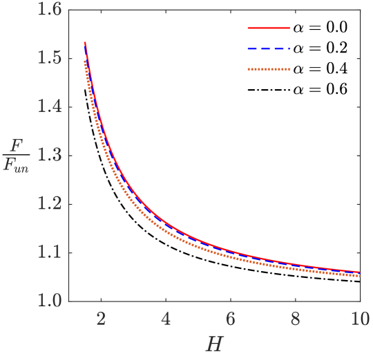
Figure 5: Variation of external point force (parallel to the wall) given in (61) relative to the unbounded given in (59) for different wall-particle gap widths, H varying from 1.5 to 10 at $\tilde{\rho}=1.05$, $K_{fz}=0.5$ and $\gamma=2$.

The deformed shape of the particle at different values of $\gamma$ for fixed $H$ value at $\alpha=0.2$ is shown in figure 6(a). As expected, particles with larger $\gamma$ exhibit reduced volumetric deformation compared to those with lower $\gamma$. Figure 6(b) illustrates the variation of deformed shape with $H$ at a constant $\gamma$. As $H$ decreases, the particle experiences greater flow resistance, and the asymmetry in the deformed shape increases.

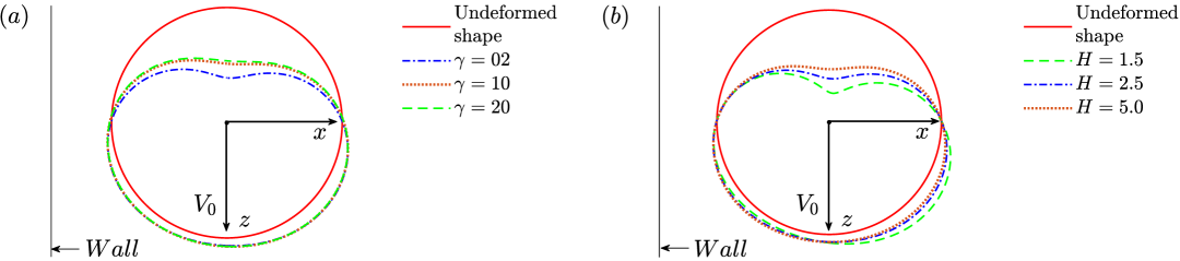
Figure 6: Variation in the shape of the deformed sphere on $xz$ plane at $\alpha=0.2$; (a) for different values of $\gamma$ at $H=2.5$ and (b) for different values of $H$ at $\gamma=2$.

The point force for a neutrally buoyant particle can be obtained by equating the particle and fluid densities at the leading-order in (61) and is obtained as

$$\mathbf{F}_{nb} =6\pi\mu V_{0}R_{0}\left[\left(1+\frac{9}{16H}+\frac{81}{256H^{2}}+\frac{217}{4096H^{3}}\right)\mathbf{\hat{k}}-\alpha\left(\frac{9}{64H^{2}}\right)\mathbf{\hat{i}}+\alpha^{2}\left(E_{1}\left[1+\frac{9}{4H}\right]+\right.\right.$$

$$\left.\left.K_{fz}^{3}\,E_{2}+K_{fz}^{2}\left(E_{3}-\frac{27(8+69\gamma+10\gamma^{2})}{160(2+\gamma)\,H}\right)E_{2}+K_{fz}\left[E_{4}E_{2}+\frac{E_{5}}{H}\right]\right)\mathbf{\hat{k}}\right].$$ (62)

Here,

$$E_{5}=-\frac{9(1792+6354\gamma+7213\gamma^{2}+2922\gamma^{3}+475\gamma^{4})}{64(2+\gamma)(2+3\gamma)^{2}(14+19\gamma)}.$$ (63)

It is worth noting that even a neutrally buoyant particle experiences a buoyancy force at O($\alpha^{2}$) due to its compressibility. In the absence of gravity or when $K_{fz}\ll 1$, a limit relevant for microfluidic devices, (61) simplified further and one gets the force as

$$\mathbf{F}_{0g}=6\pi\mu V_{0}R_{0}\left[\left(1+\frac{9}{16H}+\frac{81}{256H^{2}}+\frac{217}{4096H^{3}}\right)\mathbf{\hat{k}}-\alpha\left(\frac{9}{64H^{2}}\right)\mathbf{\hat{i}}+\alpha^{2}E_{1}\left(1+\frac{9}{4H}\right)\mathbf{\hat{k}}\right].$$ (64)

III.2 Gravity in an arbitrary direction

Here, we present the point force and the point torque for the case of the particle translating parallel to the wall and gravity is in an arbitrary direction ($\mathbf{g}=g_{x}\mathbf{\hat{i}}+g_{y}\mathbf{\hat{j}}+g_{z}\mathbf{\hat{k}}$). Following the procedure outlined in section II.5, we first calculated the variables in an unbounded domain and then accounted for wall effects using the method of reflections. Due to the misalignment between gravity and the particle velocity, the deformed shape of the particle lacks symmetry about the $z$-axis even in the unbounded domain. The point forces in unbounded and semi-infinite domains for arbitrary gravity, are represented by $\mathbf{F}_{un,ag}$ and $\mathbf{F}_{ag}$, respectively. The force in the unbounded domain is obtained as

$$\mathbf{F}_{un,ag} =6\pi\mu V_{0}R_{0}\left(\ \left[\left(1+\frac{2K_{fz}}{9}\left[1-\tilde{\rho}\right]\right)\mathbf{\hat{k}}+\frac{2[1-\tilde{\rho}]}{9}\left(K_{fx}\mathbf{\mathbf{\hat{i}}}+K_{fy}\mathbf{\hat{j}}\right)\right]+\right.$$

$$\left.\alpha^{2}\left[F^{(2)}_{un,ag_{x}}\mathbf{\hat{i}}+F^{(2)}_{un,ag_{y}}\mathbf{\hat{j}}+F^{(2)}_{un,ag_{z}}\mathbf{\hat{k}}\right]\ \right).$$ (65)

Above, the Cartesian components of the force coefficient at O($\alpha^{2}$), denoted as $F^{(2)}_{un,ag_{i}}$, ($i=x,y,z$), are given in the Appendix C. Note that the force at O($\alpha^{2}$) along $z$-direction is a function of $K_{fx}$, $K_{fy}$, $K_{fz}$, $\gamma$, and $\tilde{\rho}$ and is not the same as that at O($\alpha^{2}$) in (59), where it is only a function of $K_{fz}$, $\gamma$, and $\tilde{\rho}$. Therefore, the body forces in $x$- and $y$-directions also affect the force in the $z$-direction in the arbitrary gravity case, due to the non-linearity in the boundary conditions. Further, the torque comes at O($\alpha$) and is obtained as

$$\mathbf{T}_{un,ag}=8\pi\mu V_{0}R_{0}^{2}\left(\alpha\left[\frac{2-2\gamma(1-\tilde{\rho})+\tilde{\rho}}{8(2+3\gamma)}\left(-K_{fy}\mathbf{\mathbf{\hat{i}}}+K_{fx}\mathbf{\hat{j}}\right)\right]\ \right).$$ (66)

Due to the elastic effects, the torque appears at O($\alpha$) in this case, while it is zero when gravity is aligned with the particle velocity.

The simplified form of the point force ($\mathbf{F}^{x}_{un,ag}$) and the point torque ($\mathbf{T}^{x}_{un,ag}$) when gravity acts along the $x$-axis ($\mathbf{g}=g_{x}\mathbf{\hat{i}}$) is obtained by substituting $K_{fy}=K_{fz}=0$ in (65) and (66), respectively. The point force is obtained as

$$\mathbf{F}^{x}_{un,ag} =6\pi\mu V_{0}R_{0}\left(\ \left[1\,\mathbf{\hat{k}}+\frac{2(1-\tilde{\rho})}{9}K_{fx}\mathbf{\mathbf{\hat{i}}}\right]+\alpha^{2}\left[F^{(2),x}_{un,ag_{x}}\mathbf{\hat{i}}+F^{(2),x}_{un,ag_{z}}\mathbf{\hat{k}}\right]\ \right).$$ (67)

Here,

$$F^{(2),x}_{un,ag_{x}}=\frac{-1}{144(2+\gamma)(2+3\gamma)^{2}(14+19\gamma)}\left(8K_{fx}^{3}[14+19\gamma]J_{1}+9K_{fx}J_{2}\right),$$

$$F^{(2),x}_{un,ag_{z}}=E_{1}+K_{fx}^{2}J_{3},$$

$$J_{1}=18+\gamma(45+\gamma(16+\gamma))-32\tilde{\rho}-2\gamma(33+\gamma(12+\gamma))\tilde{\rho}+(10+\gamma(19+\gamma(8+\gamma)))\tilde{\rho}^{2},$$

$$J_{2}=28(83+30\tilde{\rho})+\gamma(7008+3672\tilde{\rho}+\gamma(6551+5658\tilde{\rho}+\gamma(2010+287\gamma+3504\tilde{\rho}+663\gamma\tilde{\rho}))),$$

$$J_{3}=\frac{1}{40(2+\gamma)(2+3\gamma)^{2}(14+19\gamma)}[-217\gamma^{4}(-1+\tilde{\rho})^{2}-2\gamma^{3}(-1+\tilde{\rho})(-891+665\tilde{\rho})+$$

$$\gamma^{2}(-4609+(7564-2803\tilde{\rho})\tilde{\rho})-28(33+\tilde{\rho}(-64+23\tilde{\rho}))-8\gamma(471+\tilde{\rho}(-811+288\tilde{\rho}))],$$ (68)

and the point torque is obtained as

$$\mathbf{T}^{x}_{un,ag}=8\pi\mu V_{0}R_{0}^{2}\left(\alpha\left[\frac{2-2\gamma(1-\tilde{\rho})+\tilde{\rho}}{8(2+3\gamma)}K_{fx}\mathbf{\hat{j}}\right]\ \right).$$ (69)

Above, superscript $()^{x}$ denotes the gravity is in the $x$-direction. Due to the non-linearity in the boundary conditions, the point force at O($\alpha^{2}$) in the $z$-direction depends on the gravitational force in the $x$-direction, as given in (67).

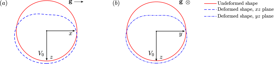
Figure 7: Variation in the shape of the deformed sphere in the unbounded domain at $K_{fx}=2$, $\alpha=0.2$, $\gamma=2$ and $\tilde{\rho}=1.05$ on (a) $xz$ plane and (b) $yz$ plane.

To illustrate the effect of gravitational force orientation on particle deformation, we plotted the deformed shape in an unbounded domain on the $xz$ and $yz$ planes when gravity is perpendicular to the particle velocity. When gravity acts along the $x$-axis, the shape on the $xz$ and $yz$ planes is shown in figure 7(a) and (b), respectively. On the plane $y=0$, the deformed shape remains symmetric about the $z$-axis in the absence of gravity. However, when gravity acts in the $x$-direction, perpendicular to the velocity of the particle, the deformed shape becomes asymmetric about the $z$-axis. This causes a shift in the centroid of the particle relative to that of the undeformed shape, generating a fluid-induced moment on the particle. This moment is balanced by the external point torque, which makes the particle torque-free. However, on the plane $x=0$, the deformed shape remains symmetric about the $z$-axis, consistent with the symmetry of the surrounding flow field.

We then analysed the wall effects on the particle dynamics for the arbitrary gravity case. In the presence of the wall, the velocity and displacement fields are calculated at orders $1/H$, $\alpha/H$, and $1/H^{2}$. The point force till the order we considered is obtained as

$$\mathbf{F}_{ag} =\mathbf{F}_{un,ag}+6\pi\mu V_{0}R_{0}\left[\left(\frac{9}{16H}+\frac{81}{256H^{2}}\right)\mathbf{\hat{k}}\right].$$ (70)

The force at O($\alpha/H$) is 0 and the point torque is obtained as

$$\mathbf{T}_{ag}=\mathbf{T}_{un,ag}\left[1+\frac{9}{16H}\right].$$ (71)

The first effects of the wall appear as a torque at O($\alpha/H$) in this case as opposed to a lift at O($\alpha/H^{2}$) in (61).

IV Summary

In this paper, we have investigated the dynamics of a weakly elastic spherical particle translating parallel to a rigid wall in a quiescent fluid in the limit, $\alpha\ll 1$. The analysis is presented for two cases: first, when the gravity is aligned with particle velocity and second, when the gravity is in an arbitrary direction. For the first case, we have considered three reflections from the wall. The velocity and displacement fields calculated at orders $1/H$, $\alpha/H$, $\alpha^{2}/H$, $1/H^{2}$, $\alpha/H^{2}$, and $1/H^{3}$ are presented in section III.1. The external point force needed to make the particle translate in an unbounded domain and parallel to the wall are given in (59) and (61), respectively. In the unbounded domain, the effects of elasticity appear as a drag at O($\alpha^{2}$), and the external force is aligned with gravity ($z$-axis). The external point torque is zero till the order we considered in our calculation. A hydrodynamic lift arises due to the wall effects(away from the wall) at O($\alpha/H^{2}$). For a neutrally buoyant particle, the force expression (62) highlights the emergence of buoyancy force at O($\alpha^{2}$) due to the compressibility of the particle. The expression in the limit of $K_{fz}\ll 1$ is given in (64). The force provided in the equation is particularly relevant for microfluidic devices, where one expects $K_{fz}\ll 1$. Figure 2 shows the deformed shape of the particle in the unbounded domain and in the presence of the wall. The deformed shape is symmetric about the translation velocity ($z$-axis) in the unbounded domain, whereas it is asymmetric in the presence of the wall. The particle shape depends on the density ratio ($\tilde{\rho}$). For a heavier (lighter) particle, increasing $K_{fz}$ reduces (increases) the required external force and decreases (increases) the dip in the particle’s upper section seen in figure 3. For the second case, when gravity and particle velocity are not aligned, we considered two reflections from the wall. The velocity and displacement fields are calculated at orders $1/H$, $\alpha/H$, and $1/H^{2}$. The external force and torque needed to translate the particle are given in (70) and (71), respectively. It is noted that for this case, the torque given in (66) comes at O($\alpha$) in an unbounded domain, which is absent in the first case. Further, the elastic induced wall effects appear as torque at O($\alpha/H$) as given in (71) for this case, in contrast to lift at O($\alpha/H^{2}$) given in (61) for the former case.

The linearity of Stokes flow allows one to derive a relationship between the hydrodynamic forces and torques on a particle and its translational and angular velocities through resistance and mobility formulations. The resistance problem, fundamental for determining hydrodynamic forces and torques with prescribed particle velocity, is particularly relevant in scenarios with imposed boundary conditions. Conversely, the mobility problem determines particle motion from applied forces and torques. These formulations are inverse to each other when the particle shape is the same. In both the resistance and mobility problems, the particle is in a state of dynamic equilibrium. To solve the problems, a knowledge of the force distribution that leads to the equilibrium is not needed for a rigid particle; however, in the case of an elastic particle, the knowledge becomes crucial. Notably, the deformed shape of an elastic particle depends on the distribution. The resistance problem of a weakly deformable particle moving parallel to a wall has been solved for both unbounded and semi-infinite domains in this work. In the unbounded case, our results differ from Murata (murata1980deformation, ), which employs a mobility formulation. While Murata predicts a prolate spheroid shape at O($\alpha^{2}$), our particle shape, shown in figure 2(a), is distinct. The difference arises from the varying force distributions. Further, our approach considers the effect of particle compressibility on density, which is not considered in Murata’s analysis. We have revisited Murata’s calculation considering density change and the results are presented in the Appendix D. Our findings highlight the importance of force distribution in determining the steady-state morphology of deformable particles moving in a fluid. Therefore, identifying the force distribution acting on a deformable particle is essential for analysing its dynamics. Our analysis plays a crucial role in understanding the fluid-particle interaction and in locating the equilibrium position of an elastic particle in a microchannel, which further helps in the efficient design of cell-sorting-based microfluidic devices.

Appendix A Solutions to the Navier elasticity equations for a point force and a point torque

The governing equation for an infinite linear, isotropic and homogeneous elastic medium acted upon by a point force at $\mathbf{x=0}$ is given by

$$\mathbf{[}\lambda+G]\mathbf{\nabla}\left(\mathbf{\nabla}\cdot\mathbf{u}^{p_{f}}\right)+G\mathbf{\nabla}^{2}\mathbf{u}^{p_{f}}+\mathbf{F}\delta(\mathbf{x})={0}.$$ (72)

Above, the displacement field ($\mathbf{u}^{p_{f}}$) is due to the point force and is given by

$$\mathbf{u}^{p_{f}}(\mathbf{x}) =\boldsymbol{G}(\mathbf{x})\cdot\mathbf{F}$$

$$=\frac{1}{16(1-\nu)\pi G}\left[\frac{\mathbf{I}(3-4\nu)}{r}+\frac{\mathbf{x}\mathbf{x}}{r^{3}}\right]\cdot\mathbf{F}\,.$$ (73)

Here, $r=|\mathbf{x}|$, $\boldsymbol{G}(\mathbf{x})$ is the Green’s function and $\nu=\lambda/(2[\lambda+G])$ is the Poisson ratio. It can be shown that (73) is indeed the solution by substituting it in (72) and integrating over any volume ($\mathring{V}$) enclosing point force. Using the divergence theorem, the integration yields

$$\int_{\mathring{V}}\left(\mathbf{[}\lambda+G]\mathbf{\nabla}\left(\mathbf{\nabla}\cdot\mathbf{u}^{p_{f}}\right)+G\mathbf{\nabla}^{2}\mathbf{u}^{p_{f}}\right)dV=-\mathbf{F}\,.$$ (74)

One can derive the displacement field corresponding to a point torque by drawing an analogy to the rotlet singularity in the case of the Stokes equation (kim2013microhydrodynamics, ). The governing equation for an infinite elastic medium with point torque at $\mathbf{x=0}$ is given by

$$\mathbf{[}\lambda+G]\mathbf{\nabla}\left(\mathbf{\nabla}\cdot\mathbf{u}^{p_{t}}\right)+G\mathbf{\nabla}^{2}\mathbf{u}^{p_{t}}+\frac{1}{2}\left[\mathbf{\nabla}\delta(\mathbf{x})\times\mathbf{T}\right]={0}\,.$$ (75)

Above, the displacement field ($\mathbf{u}^{p_{t}}$) is due to the point torque and is given by

$$\mathbf{u}^{p_{t}}(\mathbf{x})=\frac{\mathbf{T}\times\mathbf{x}}{8\pi Gr^{3}}\,.$$ (76)

One can verify that the displacement field is indeed correct by substituting (76) in (75) and taking its moment about the origin and integrating over an arbitrary volume ($\mathring{V}$) enclosing the point torque. Using the divergence theorem, the integration yields

$$\int_{\mathring{V}}\mathbf{x}\times\left(\mathbf{[}\lambda+G]\mathbf{\nabla}\left(\mathbf{\nabla}\cdot\mathbf{u}^{p_{t}}\right)+G\mathbf{\nabla}^{2}\mathbf{u}^{p_{t}}\right)dV=-\mathbf{T}\,.$$ (77)

The displacement field corresponding to the point force and the point torque decays as $r^{-1}$ and $r^{-2}$, respectively.

Appendix B Gravity aligned with particle velocity

The radial ($v^{(2)}_{un,r}$) and tangential ($v^{(2)}_{un,\theta}$) velocity components at O($\alpha^{2}$) for the case when gravity is in $z$-direction are obtained as

$$v^{(2)}_{un,r} =-\frac{3\cos\theta}{320(2+\gamma)^{2}(2+3\gamma)^{2}(14+19\gamma)\xi^{5}}[-((-1+\xi^{2})(45(-1120\xi^{2}+\gamma(368-3440\xi^{2})+$$

$$\gamma^{3}(1881-860\xi^{2})+8\gamma^{4}(131+4\xi^{2})+\gamma^{5}(177+4\xi^{2})-22\gamma^{2}(-63+148\xi^{2}))-60K_{fz}($$

$$3\gamma^{5}(23+28\xi^{2})(-1+\tilde{\rho})-112(2+\xi^{2}(-3+2\tilde{\rho}))+6\gamma^{2}(-197+63\tilde{\rho}+6\xi^{2}(17+6\tilde{\rho}))+$$

$$\gamma(-824+92\tilde{\rho}-64\xi^{2}(-16+7\tilde{\rho}))+\gamma^{4}(-400+358\tilde{\rho}+8\xi^{2}(-59+65\tilde{\rho}))+\gamma^{3}(-901+$$

$$570\tilde{\rho}+\xi^{2}(-516+896\tilde{\rho})))+4K_{fz}^{2}(\gamma^{5}(81+244\xi^{2})(-1+\tilde{\rho})^{2}+8\gamma^{4}(-1+\tilde{\rho})(-66+39\tilde{\rho}+$$

$$\xi^{2}(-109+186\tilde{\rho}))-4\gamma(-340+586\tilde{\rho}+51\tilde{\rho}^{2}+4\xi^{2}(315-349\tilde{\rho}+\tilde{\rho}^{2}))-56(-4+12\tilde{\rho}+$$

$$\tilde{\rho}^{2}+4\xi^{2}(6-8\tilde{\rho}+\tilde{\rho}^{2}))+2\gamma^{2}(1149-1474\tilde{\rho}-80\tilde{\rho}^{2}+36\xi^{2}(-74+54\tilde{\rho}+25\tilde{\rho}^{2}))+\gamma^{3}($$

$$3(503-628\tilde{\rho}+68\tilde{\rho}^{2})+4\xi^{2}(-201-499\tilde{\rho}+719\tilde{\rho}^{2})))))+5(9(2800\xi^{2}+40\gamma(-46+365\xi^{2})$$

$$+8\gamma^{4}(-655+1319\xi^{2})+\gamma^{5}(-885+1493\xi^{2})+\gamma^{3}(-9405+25757\xi^{2})+\gamma^{2}(-6930+$$

$$28498\xi^{2}))-12K_{fz}(\gamma^{5}(-345+649\xi^{2})(-1+\tilde{\rho})+560(2+\xi^{2}(-3+2\tilde{\rho}))+2\gamma^{4}(1000-$$

$$895\tilde{\rho}+\xi^{2}(-2176+2147\tilde{\rho}))+2\gamma^{2}(2955-945\tilde{\rho}+\xi^{2}(-6439+5563\tilde{\rho}))+\gamma(4120-460\tilde{\rho}+$$

$$\xi^{2}(-7456+5732\tilde{\rho}))+\gamma^{3}(4505-2850\tilde{\rho}+\xi^{2}(-10785+10154\tilde{\rho})))+4K_{fz}^{2}(\gamma^{5}(-81+$$

$$233\xi^{2})(-1+\tilde{\rho})^{2}+8\gamma^{4}(-1+\tilde{\rho})(66-39\tilde{\rho}+2\xi^{2}(-97+93\tilde{\rho}))+56(-4+12\tilde{\rho}+\tilde{\rho}^{2}+\xi^{2}($$

$$6-20\tilde{\rho}+7\tilde{\rho}^{2}))+4\gamma(-340+586\tilde{\rho}+51\tilde{\rho}^{2}+\xi^{2}(546-1270\tilde{\rho}+493\tilde{\rho}^{2}))+2\gamma^{2}(-1149+$$

$$1474\tilde{\rho}+80\tilde{\rho}^{2}+\xi^{2}(2221-4430\tilde{\rho}+1894\tilde{\rho}^{2}))+\gamma^{3}(-3(503-628\tilde{\rho}+68\tilde{\rho}^{2})+\xi^{2}(3853-$$

$$7444\tilde{\rho}+3458\tilde{\rho}^{2}))))\cos(2\theta)],$$ (78)

and

$$v^{(2)}_{un,\theta} =-\frac{3}{1280(2+\gamma)^{2}(2+3\gamma)^{2}(14+19\gamma)\xi^{5}}[45(560\xi^{2}(1-4\xi^{2})+\gamma^{3}(-16929+20275\xi^{2}-$$

$$1720\xi^{4})+8\gamma^{4}(-1179+1065\xi^{2}+8\xi^{4})+\gamma^{5}(-1593+1147\xi^{2}+8\xi^{4})-8\gamma(414-873\xi^{2}+$$

$$860\xi^{4})-2\gamma^{2}(6237-9607\xi^{2}+3256\xi^{4}))-60K_{fz}(\gamma^{5}(-621+679\xi^{2}+168\xi^{4})(-1+\tilde{\rho})-$$

$$112(-18+\xi^{2}(5-6\tilde{\rho})+\xi^{4}(-6+4\tilde{\rho}))-4\gamma(\xi^{2}(940-1163\tilde{\rho})+32\xi^{4}(-16+7\tilde{\rho})+9(-206$$

$$+23\tilde{\rho}))+2\gamma^{4}(1800-1611\tilde{\rho}+8\xi^{4}(-59+65\tilde{\rho})+\xi^{2}(-2248+2309\tilde{\rho}))+2\gamma^{2}(5319-$$

$$1701\tilde{\rho}+36\xi^{4}(17+6\tilde{\rho})+\xi^{2}(-4645+5401\tilde{\rho}))+\gamma^{3}(8109-5130\tilde{\rho}+8\xi^{4}(-129+224\tilde{\rho})+$$

$$\xi^{2}(-10015+10806\tilde{\rho})))+4K_{fz}^{2}(\gamma^{5}(-729+1491\xi^{2}+488\xi^{4})(-1+\tilde{\rho})^{2}+8\gamma^{4}(-1+\tilde{\rho})$$

$$(594-351\tilde{\rho}+24\xi^{2}(-44+51\tilde{\rho})+\xi^{4}(-218+372\tilde{\rho}))-56(\xi^{2}(26+12\tilde{\rho}-29\tilde{\rho}^{2})+8\xi^{4}($$

$$6-8\tilde{\rho}+\tilde{\rho}^{2})-9(-4+12\tilde{\rho}+\tilde{\rho}^{2}))-4\gamma(\xi^{2}(470+2386\tilde{\rho}-2559\tilde{\rho}^{2})+8\xi^{4}(315-349\tilde{\rho}+$$

$$\tilde{\rho}^{2})-9(-340+586\tilde{\rho}+51\tilde{\rho}^{2}))+2\gamma^{2}(72\xi^{4}(-74+54\tilde{\rho}+25\tilde{\rho}^{2})+9(-1149+1474\tilde{\rho}+$$

$$80\tilde{\rho}^{2})+\xi^{2}(3479-15314\tilde{\rho}+11430\tilde{\rho}^{2}))+\gamma^{3}(-27(503-628\tilde{\rho}+68\tilde{\rho}^{2})+8\xi^{4}(-201-499\tilde{\rho}$$

$$+719\tilde{\rho}^{2})+\xi^{2}(14639-37444\tilde{\rho}+22634\tilde{\rho}^{2})))+5(9(2800\xi^{2}+40\gamma(-138+365\xi^{2})+8\gamma^{4}($$

$$-1965+1319\xi^{2})+\gamma^{5}(-2655+1493\xi^{2})+\gamma^{3}(-28215+25757\xi^{2})+\gamma^{2}(-20790+$$

$$28498\xi^{2}))-12K_{fz}(\gamma^{5}(-1035+649\xi^{2})(-1+\tilde{\rho})+560(6+\xi^{2}(-3+2\tilde{\rho}))+4\gamma(3090-$$

$$345\tilde{\rho}+\xi^{2}(-1864+1433\tilde{\rho}))+\gamma^{4}(6000-5370\tilde{\rho}+\xi^{2}(-4352+4294\tilde{\rho}))+2\gamma^{2}(8865-$$

$$2835\tilde{\rho}+\xi^{2}(-6439+5563\tilde{\rho}))+\gamma^{3}(13515-8550\tilde{\rho}+\xi^{2}(-10785+10154\tilde{\rho})))+4K_{fz}^{2}($$

$$\gamma^{5}(-243+233\xi^{2})(-1+\tilde{\rho})^{2}+8\gamma^{4}(-1+\tilde{\rho})(198-117\tilde{\rho}+2\xi^{2}(-97+93\tilde{\rho}))+56(3(-4+$$

$$12\tilde{\rho}+\tilde{\rho}^{2})+\xi^{2}(6-20\tilde{\rho}+7\tilde{\rho}^{2}))+4\gamma(3(-340+586\tilde{\rho}+51\tilde{\rho}^{2})+\xi^{2}(546-1270\tilde{\rho}+493\tilde{\rho}^{2}))$$

$$+\gamma^{3}(-9(503-628\tilde{\rho}+68\tilde{\rho}^{2})+\xi^{2}(3853-7444\tilde{\rho}+3458\tilde{\rho}^{2}))+\gamma^{2}(-6894+8844\tilde{\rho}+$$

$$480\tilde{\rho}^{2}+\xi^{2}(4442-8860\tilde{\rho}+3788\tilde{\rho}^{2}))))\cos(2\theta)]\sin\theta.$$ (79)

The expressions for $E_{1}$, $E_{2}$, $E_{3}$, $E_{4}$, $I_{1}$, $I_{2}$, $I_{3}$, $I_{4}$ and $I_{5}$ in (59) and (61) for both the unbounded and semi-infinite case are obtained as

$$E_{1}=\frac{9(-140-360\gamma-227\gamma^{2}+6\gamma^{3}+\gamma^{4})}{8(2+\gamma)(2+3\gamma)^{2}(14+19\gamma)},\ E_{2}=\frac{28+52\gamma+19\gamma^{2}}{9(2+\gamma)(2+3\gamma)^{2}(14+19\gamma)},$$ (80)

$$E_{3}=-\frac{3(7+\gamma)(1+5\gamma)}{5(2+\gamma)},\ E_{4}=-\frac{9(1708+5964\gamma+6787\gamma^{2}+2850\gamma^{3}+475\gamma^{4})}{8(28+52\gamma+19\gamma^{2})},$$ (81)

$$I_{1}=-\frac{\gamma^{3}(1-\tilde{\rho})^{2}+8\gamma^{2}(2-3\tilde{\rho}+\tilde{\rho}^{2})+2(9-16\tilde{\rho}+5\tilde{\rho}^{2})+\gamma(45-66\tilde{\rho}+19\tilde{\rho}^{2})}{2(2+\gamma)},$$ (82)

$$I_{2}=\frac{1}{2(7+\gamma)(1+5\gamma)(14+19\gamma)}\left[\gamma^{3}(3102-2162\tilde{\rho}-750\tilde{\rho}^{2})+\gamma^{2}(10734-8569\tilde{\rho}-\right.$$

$$\left.657\tilde{\rho}^{2})+\gamma^{4}(292-109\tilde{\rho}-183\tilde{\rho}^{2})+28(108-104\tilde{\rho}+3\tilde{\rho}^{2})-2\gamma(-5224+4569\tilde{\rho}+18\tilde{\rho}^{2})\right],$$ (83)

$$I_{3}=\frac{2044-336\tilde{\rho}-84\gamma(-77+6\tilde{\rho})+6\gamma^{3}(299+176\tilde{\rho})+\gamma^{4}(223+252\tilde{\rho})+\gamma^{2}(6211+576\tilde{\rho})}{1708+5964\gamma+6787\gamma^{2}+2850\gamma^{3}+475\gamma^{4}},$$ (84)

$$I_{4}=\frac{27}{160(28+52\gamma+19\gamma^{2})}\left(\gamma^{4}(-1+\tilde{\rho})(109+366\tilde{\rho})+2\gamma^{3}(-1407+562\tilde{\rho}+750\tilde{\rho}^{2})-\right.$$

$$\left.56(63+\tilde{\rho}(-64+3\tilde{\rho}))+2\gamma(-6043+12\tilde{\rho}(454+3\tilde{\rho}))+\gamma^{2}(-11913+2\tilde{\rho}(4574+657\tilde{\rho}))\right),$$ (85)

$$I_{5}=-\frac{9}{64(2+\gamma)(2+3\gamma)^{2}(14+19\gamma)}\left(\gamma(7110-756\tilde{\rho})+56(41-9\tilde{\rho})+6\gamma^{3}(223+264\tilde{\rho})+\right.$$

$$\left.\gamma^{4}(97+378\tilde{\rho})+\gamma^{2}(6349+864\tilde{\rho})\right).$$ (86)

The expressions for $B_{1}$, $B_{2}$, $B_{3}$, $B_{4}$ and $B_{5}$ in (60) are obtained as

$$B_{1}=\frac{27(5+8\gamma+2\gamma^{2})}{32(2+\gamma)(2+3\gamma)},\ B_{2}=-\frac{81(7840+33504\gamma+53806\gamma^{2}+40067\gamma^{3}+13704\gamma^{4}+1739\gamma^{5})}{512(2+\gamma)^{2}(2+3\gamma)^{2}(14+19\gamma)},$$ (87)

$$B_{3}=\frac{27}{256(2+\gamma)^{2}(2+3\gamma)^{2}(14+19\gamma)}\left(647\gamma^{5}(-1+\tilde{\rho})+224(-11+12\tilde{\rho})+4\gamma(-2798+\right.$$

$$\left.2929\tilde{\rho})+\gamma^{4}(-4960+5042\tilde{\rho})+2\gamma^{2}(-9353+9587\tilde{\rho})+\gamma^{3}(-14231+14526\tilde{\rho})\right),$$ (88)

$$B_{4}=-\frac{81(5600+27360\gamma+50066\gamma^{2}+42109\gamma^{3}+15864\gamma^{4}+2101\gamma^{5})}{512(2+\gamma)^{2}(2+3\gamma)^{2}(14+19\gamma)},$$ (89)

$$B_{5}=\frac{27}{256(2+\gamma)^{2}(2+3\gamma)^{2}(14+19\gamma)}\left(2240(-1+\tilde{\rho})+953\gamma^{5}(-1+\tilde{\rho})+4\gamma(-2698+\right.$$

$$\left.2751\tilde{\rho})+\gamma^{4}(-6704+6798\tilde{\rho})+2\gamma^{2}(-9923+10181\tilde{\rho})+\gamma^{3}(-17065+17458\tilde{\rho})\right).$$ (90)

Appendix C Gravity in an arbitrary direction

The expression for the components of force coefficient at O($\alpha^{2}$) given in (65) where gravity is in the arbitrary direction ($\mathbf{g}=g_{x}\mathbf{\hat{i}}+g_{y}\mathbf{\hat{j}}+g_{z}\mathbf{\hat{k}}$) are obtained as

$$F^{(2)}_{un,ag_{x}} =\frac{K_{fx}}{720(2+\gamma)(2+3\gamma)^{2}(14+19\gamma)}(\gamma[-45\gamma(6551+\gamma(2010+287\gamma))-$$

$$40K_{fz}^{2}(972+\gamma(1079+\gamma(318+19\gamma)))-6K_{fz}(30488+\gamma(29109+$$

$$11\gamma(642+47\gamma)))]+(80K_{fz}^{2}(14+19\gamma)(16+\gamma(33+\gamma(12+\gamma)))-$$

$$135\gamma(1224+\gamma(1886+\gamma(1168+221\gamma)))-12K_{fz}(-3136+\gamma(-8544+$$

$$\gamma(-5792+\gamma(344+433\gamma)))))\tilde{\rho}+2K_{fz}[-20K_{fz}(14+19\gamma)(10+\gamma(19+$$

$$\gamma(8+\gamma)))+9(532+\gamma(2352+\gamma(3679+\gamma(2330+461\gamma))))]\tilde{\rho}^{2}-$$

$$36(2905+1554K_{fz}+280K_{fz}^{2}+8760\gamma+1050\tilde{\rho})-40K_{fx}^{2}(14+19\gamma)(18+$$

$$\gamma(45+\gamma(16+\gamma))-32\tilde{\rho}-2\gamma(33+\gamma(12+\gamma))\tilde{\rho}+(10+\gamma(19+\gamma(8+\gamma)))\tilde{\rho}^{2})-$$

$$40K_{fy}^{2}(14+19\gamma)(18+\gamma(45+\gamma(16+\gamma))-32\tilde{\rho}-2\gamma(33+\gamma(12+\gamma))\tilde{\rho}+$$

$$(10+\gamma(19+\gamma(8+\gamma)))\tilde{\rho}^{2})),$$ (91)

$$F^{(2)}_{un,ag_{y}}=\frac{K_{fy}}{K_{fx}}\left[F^{(2)}_{un,ag_{x}}\right],$$ (92)

$$F^{(2)}_{un,ag_{z}} =-\frac{1}{360(2+\gamma)(2+3\gamma)^{2}(14+19\gamma)}(8316K_{fy}^{2}+5040K_{fy}^{2}K_{fz}+36288K_{fz}^{2}+5040K_{fz}^{3}$$

$$+33912K_{fy}^{2}\gamma+291060K_{fz}\gamma+19440K_{fy}^{2}K_{fz}\gamma+125376K_{fz}^{2}\gamma+19440K_{fz}^{3}\gamma+91935\gamma^{2}$$

$$+41481K_{fy}^{2}\gamma^{2}+279495K_{fz}\gamma^{2}+21580K_{fy}^{2}K_{fz}\gamma^{2}+128808K_{fz}^{2}\gamma^{2}+21580K_{fz}^{3}\gamma^{2}$$

$$-2430\gamma^{3}+16038K_{fy}^{2}\gamma^{3}+80730K_{fz}\gamma^{3}+6360K_{fy}^{2}K_{fz}\gamma^{3}+37224K_{fz}^{2}\gamma^{3}+6360K_{fz}^{3}\gamma^{3}$$

$$-405\gamma^{4}+1953K_{fy}^{2}\gamma^{4}+10035K_{fz}\gamma^{4}+380K_{fy}^{2}K_{fz}\gamma^{4}+3504K_{fz}^{2}\gamma^{4}+380K_{fz}^{3}\gamma^{4}$$

$$+180(315+511K_{fz}+810\gamma)-2(2K_{fz}(10K_{fz}^{2}(14+19\gamma)(16+\gamma(33+\gamma(12+\gamma)))$$

$$-135(-28+\gamma(-42+\gamma(48+\gamma(88+21\gamma))))+3K_{fz}(2912+\gamma(9138+\gamma(8569+$$

$$\gamma(2162+109\gamma)))))+K_{fy}^{2}(20K_{fz}(14+19\gamma)(16+\gamma(33+\gamma(12+\gamma)))+9(896+$$

$$\gamma(3244+\gamma(3782+\gamma(1556+217\gamma))))))\tilde{\rho}+(4K_{fz}^{2}(252+5K_{fz}(14+19\gamma)(10+$$

$$\gamma(19+\gamma(8+\gamma)))-9\gamma(12+\gamma(219+\gamma(250+61\gamma))))+K_{fy}^{2}(20K_{fz}(14+19\gamma)(10+$$

$$\gamma(19+\gamma(8+\gamma)))+9(644+\gamma(2304+\gamma(2803+7\gamma(190+31\gamma))))))\tilde{\rho}^{2}+K_{fx}^{2}$$

$$(20K_{fz}(14+19\gamma)(18+\gamma(45+\gamma(16+\gamma))-32\tilde{\rho}-2\gamma(33+\gamma(12+\gamma))\tilde{\rho}+(10+$$

$$\gamma(19+\gamma(8+\gamma)))\tilde{\rho}^{2})+9(217\gamma^{4}(-1+\tilde{\rho})^{2}+2\gamma^{3}(-1+\tilde{\rho})(-891+665\tilde{\rho})+28(33+$$

$$\tilde{\rho}(-64+23\tilde{\rho}))+8\gamma(471+\tilde{\rho}(-811+288\tilde{\rho}))+\gamma^{2}(4609+\tilde{\rho}(-7564+2803\tilde{\rho}))))).$$ (93)

Appendix D Modification in the analysis of Murata (murata1980deformation, )

Murata calculated the velocity of a weakly elastic sphere sedimenting under gravity in an unbounded domain. The velocity of the particle ($V_{p}\mathbf{\hat{k}}$) is in the direction of gravity ($g_{z}\mathbf{\hat{k}}$). In our notation, the velocity can be written as an asymptotic series in $\alpha$ as

$$V_{p}=\frac{2[\tilde{\rho}-1]\rho_{f}g_{z}R_{0}^{2}}{9\mu}\left[1+\alpha^{2}V^{(2)}\right].$$ (94)

Here, $V^{(2)}$ is the velocity coefficient at O($\alpha^{2}$) and is given by

$$V^{(2)}=\frac{-27\big{(}6+\gamma[18+\gamma]\big{)}+6K_{fz}(-1+16\gamma)\tilde{\rho}+8K_{fz}^{2}\tilde{\rho}^{2}}{20(2+3\gamma)^{2}}.$$ (95)

Murata had neglected the density variation of the particle. If one includes that, the coefficient of the terminal velocity at O($\alpha^{2}$) is different from (95). The modified coefficient at O($\alpha^{2}$) is obtained as

$$V^{(2)}_{mod}=\frac{-243\big{(}6+\gamma[18+\gamma]\big{)}+18K_{fz}\big{(}32+\gamma[133+5\gamma]\big{)}\tilde{\rho}+6K_{fz}^{2}(7-50\gamma)\tilde{\rho}^{2}-20K_{fz}^{3}\tilde{\rho}^{3}}{180(2+3\gamma)^{2}}.$$ (96)

References

- (1) Secomb, Timothy W, Skalak, R, Özkaya, N & Gross, JF 1986 Flow of axisymmetric red blood cells in narrow capillaries. Journal of Fluid Mechanics 163, 405–423.
- (2) Song, Yongxin, Li, Deyu & Xuan, Xiangchun 2023 Recent advances in multi-mode microfluidic separation of particles and cells. Electrophoresis.
- (3) Wu, Ting, Yang, Zhibing, Hu, Ran, Chen, Yi-Feng, Zhong, Hua, Yang, Lei & Jin, Wenbiao 2021 Film entrainment and microplastic particles retention during gas invasion in suspension-filled microchannels. Water Research 194, 116919.
- (4) Guazzelli, Elisabeth & Morris, Jeffrey F 2011 A physical introduction to suspension dynamics. Cambridge University Press.
- (5) Goldman, Arthur Joseph, Cox, Raymond G & Brenner, Howard 1967 Slow viscous motion of a sphere parallel to a plane wall—I Motion through a quiescent fluid. Chemical Engineering Science 22(4), 637–651.
- (6) Dean, WR & O’Neill, ME 1963 A slow motion of viscous liquid caused by the rotation of a solid sphere. Mathematika 10(1), 13–24.
- (7) O’Neill, Michael E 1964 A slow motion of viscous liquid caused by a slowly moving solid sphere. Mathematika 11(1), 67–74.
- (8) Matas, JP, Morris, JF & Guazzelli, Elisabeth 2004 Lateral forces on a sphere. Oil & Gas Science and Technology 59(1), 59–70.
- (9) Saffman, Philip Geoffrey 1965 The lift on a small sphere in a slow shear flow. Journal of Fluid Mechanics 22(2), 385–400.
- (10) Anand, Prateek & Subramanian, Ganesh 2023 Inertial migration of a sphere in plane couette flow. Journal of Fluid Mechanics 977, A33.
- (11) Vasseur, P., & Cox, R.G. (1976). The lateral migration of a spherical particle in two-dimensional shear flows. Journal of Fluid Mechanics, 78(2), 385–413.
- (12) Ho, BP & Leal, LG 1974 Inertial migration of rigid spheres in two-dimensional unidirectional flows. Journal of Fluid Mechanics 65(2), 365–400.
- (13) Nakayama, S., Yamashita, H., Yabu, T., Itano, T., & Sugihara-Seki, M. (2019). Three regimes of inertial focusing for spherical particles suspended in circular tube flows. Journal of Fluid Mechanics, 871, 952–969.
- (14) Segre, G. and Silberberg, A. (1961). Radial particle displacements in Poiseuille flow of suspensions. Nature, 189(4760), 209–210.
- (15) Leal, LG 1980 Particle motions in a viscous fluid. Annual Review of Fluid Mechanics 12, 435–476.
- (16) Chaffey, CE, Brenner, H & Mason, SG 1965 Particle motions in sheared suspensions: XVIII: Wall migration (theoretical). Rheologica Acta 4(1), 64–72.
- (17) Magnaudet, Jacques, Takagi, SHU & Legendre, Dominique 2003 Drag, deformation and lateral migration of a buoyant drop moving near a wall. Journal of Fluid Mechanics 476, 115–157.
- (18) Rallabandi, Bhargav, Oppenheimer, Naomi, Ben Zion, Matan Yah & Stone, Howard A 2018 Membrane-induced hydroelastic migration of a particle surfing its own wave. Nature Physics 14(12), 1211–1215.
- (19) Rallabandi, Bhargav, Saintyves, Baudouin, Jules, Theo, Salez, Thomas, Schönecker, Clarissa, Mahadevan, L & Stone, Howard A 2017 Rotation of an immersed cylinder sliding near a thin elastic coating. Physical Review Fluids 2(7), 074102.
- (20) Daddi-Moussa-Ider, Abdallah, Rallabandi, Bhargav, Gekle, Stephan & Stone, Howard A 2018 Reciprocal theorem for the prediction of the normal force induced on a particle translating parallel to an elastic membrane. Physical Review Fluids 3(8), 084101.
- (21) Doddi, Sai K & Bagchi, Prosenjit 2009 Three-dimensional computational modeling of multiple deformable cells flowing in microvessels. Physical Review E—Statistical, Nonlinear, and Soft Matter Physics 79(4), 046318.
- (22) Barthes-Biesel, Dominique 2016 Motion and deformation of elastic capsules and vesicles in flow. Annual Review of Fluid Mechanics 48, 25–52.
- (23) Noichl, Isabell & Schönecker, Clarissa 2022 Dynamics of elastic, nonheavy spheres sedimenting in a rectangular duct. Soft Matter 18(12), 2462–2472.
- (24) Li, Shuaijun, Yu, Honghui, Li, Tai-De, Chen, Zi, Deng, Wen, Anbari, Alimohammad & Fan, Jing 2020 Understanding transport of an elastic, spherical particle through a confining channel. Applied Physics Letters 116(10), 103705.
- (25) Murata, Tadayoshi 1980 On the deformation of an elastic particle falling in a viscous fluid. Journal of the Physical Society of Japan 48(5), 1738–1745.
- (26) Nasouri, Babak, Khot, Aditi & Elfring, Gwynn J 2017 Elastic two-sphere swimmer in Stokes flow. Physical Review Fluids 2(4), 043101.
- (27) Tam, Christopher KW & Hyman, William A 1973 Transverse motion of an elastic sphere in a shear field. Journal of Fluid Mechanics 59(1), 177–185.
- (28) Kim, Sangtae & Karrila, Seppo J 2013 Microhydrodynamics: principles and selected applications. Courier Corporation.
- (29) Małysa, K & Van De Ven, TGM 1986 Rotational and translational motion of a sphere parallel to a wall. International Journal of Multiphase Flow 12(3), 459–468.
- (30) Johns, Lewis E & Narayanan, Ranga 2002 Interfacial instability. Springer Science & Business Media.
- (31) Leal, L Gary 2007 Advanced Transport Phenomena: Fluid Mechanics and Convective Transport Processes. Cambridge University Press.
- (32) Kushch, V. (2013). Micromechanics of Composites: Multipole Expansion Approach. Butterworth-Heinemann.
- (33) Faxén, H. (1923). Die Bewegung einer starren Kugel längs der Achse eines mit zäher Flüssigkeit gefüllten Rohres. Arkiv för Matematik, Astronomi och Fysik, 17, 1–28.