Attention-based Generative Latent Replay:
A Continual Learning Approach for WSI Analysis

Abstract

Whole slide image (WSI) classification has emerged as a powerful tool in computational pathology, but remains constrained by domain shifts, e.g., due to different organs, diseases, or institution-specific variations. To address this challenge, we propose an Attention-based Generative Latent Replay Continual Learning framework (AGLR-CL), in a multiple instance learning (MIL) setup for domain incremental WSI classification. Our method employs Gaussian Mixture Models (GMMs) to synthesize WSI representations and patch count distributions, preserving knowledge of past domains without explicitly storing original data. A novel attention-based filtering step focuses on the most salient patch embeddings, ensuring high-quality synthetic samples. This privacy-aware strategy obviates the need for replay buffers and outperforms other buffer-free counterparts while matching the performance of buffer-based solutions. We validate AGLR-CL on clinically relevant biomarker detection and molecular status prediction across multiple public datasets with diverse centers, organs, and patient cohorts. Experimental results confirm its ability to retain prior knowledge and adapt to new domains, offering an effective, privacy-preserving avenue for domain incremental continual learning in WSI classification.

1 Introduction

Recent advances in computational pathology (CPath) and digitizing WSIs have transformed histopathology image analysis, driving significant progress in automated disease detection and biomarker assessment. However, WSI classification remains challenging due to the gigapixel resolution and the lack of pixel-level annotations. A common strategy divides WSIs into manageable patches, which are processed offline by vision encoding models to obtain feature sequences. Notably, self-supervised pretraining has enabled the development of domain-specific foundation models (FMs) that outperform out-of-domain counterparts [23, 3, 21], such as ImageNet-pretrained models. The conversion of patch-level features into slide-level predictions is achieved through MIL by aggregation of these features.

Despite these advancements, WSI classification models still face challenges in clinical settings. Variability in morphological features, originating from differences in organ-specific biology, staining protocols, scanner manufacturers, and patient cohorts, induces distribution shifts that degrade performance on new datasets. Conventional MIL models struggle to generalize when WSIs are acquired from diverse hospitals and settings. Fine-tuning on new datasets is a common adaptation strategy; however, it often leads to catastrophic forgetting (CF) [12, 14]. On the other hand, continual learning (CL) has emerged as a promising solution for evolving medical data while mitigating CF [13, 15]. By enabling continuous knowledge accumulation, CL enhances model robustness and adaptability in clinical settings and facilitates forward knowledge transfer, e.g., from frequently stained datasets in H&E or PAS to those for follow-up diagnostics like CD8 or TRI [15]. Although buffer-based methods, which store selected past samples, typically yield superior performance [5, 1], their applicability to WSIs is hindered by storage and privacy constraints. Existing WSI CL research is limited, focusing primarily on buffer-based and class incremental methods [9, 25]. To address these limitations, we propose AGLR-CL, a buffer-free generative replay approach for domain incremental WSI classification. AGLR-CL models past domain distributions with GMMs trained on patch embeddings and counts. For each domain, class-wise multivariate GMMs and one-dimensional GMMs capture prior data distribution. In subsequent domains, synthetic data sampled from these GMMs are combined with new WSIs to update the MIL model, thus avoiding real data storage and preserving privacy. We validate AGLR-CL on multiple tasks across domain incremental datastes including various centers and organs. Extensive experiments show that AGLR-CL effectively retains prior knowledge and adapts to new domains, surpassing other buffer-free methods and achieving performance close to buffer-based methods. Our main contributions are:

(1) Domain incremental CL for MIL. To our knowledge, we introduce domain incremental CL for MIL for the first time and present a GMM and attention-based filtering for effective re-sampling of past data across domains.

(2) Broad applicability and increased privacy. Across CPath tasks, including biomarker screening and molecular status predictions, our AGLR-CL consistently surpasses buffer-free methods and is on par with buffer-based methods, while avoiding WSI storage and thus increasing privacy.

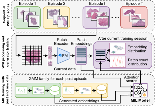
Figure 1: Privacy-aware domain incremental AGLR-CL framework. Following WSI tessellation, a frozen FM-based encoder generates a sequence of tractable embeddings. A MIL aggregator is then trained on the current episode, with high-attention features selected to fit GMMs for patch embeddings and counts. In subsequent episodes, historical data is revisited by re-sampling synthetic WSIs using the per-episode GMMs.

2 Method

A flowchart of the proposed approach is shown in Fig. 1. In the following, we detail MIL-based WSI classification, CL settings, and our AGLR-CL framework, which incorporates an attention-based selection for GMM training and synthetic embedding generation for a latent replay mechanism.

2.1 MIL-based WSI Classification

We adopt a standard preprocessing pipeline, partitioning each WSI into $n$ non-overlapping patches $p_{i}\in\mathbb{R}^{512\times 512\times 3}$. A pretrained CPath FM is then used to extract patch embeddings, resulting in a feature sequence $\{f_{i}\}_{i=1}^{n}\in\mathbb{R}^{n\times D}$, with $D$ denoting the latent dimension. These embeddings are aggregated using a learnable MIL model $\mathcal{M}$. Specifically, we employ AB-MIL [10], which embeds each feature into a lower-dimensional space $d$ via a linear layer and applies an attention mechanism to assign instance-level weights. The weighted embeddings are summed and fed into a classification head for WSI prediction.

2.2 Continual Learning Configuration

We consider a CL pipeline for WSI classification, where datasets arrive sequentially (defined as episodes), $\{\mathcal{D}_{1},\mathcal{D}_{2},\ldots,\mathcal{D}_{T}\}$, each representing a distinct domain $t\in\{1,...,T\}$. At training domain $t$, the model $\mathcal{M}$ has access to the current dataset $\mathcal{D}_{t}$ only, while evaluation is performed on test sets from all episodes $\{\mathcal{D}_{1},\mathcal{D}_{2},\ldots,\mathcal{D}_{T}\}$. Unlike approaches that retain a buffer of past samples [25, 9], our method addresses CF while avoiding WSI storage, a critical requirement in privacy-sensitive domains.

2.3 GMM-based Synthetic Embedding Generation

WSIs inherently contain a variable number of patches. To generate synthetic WSI representations, we model both the patch counts and patch embeddings using GMMs. For a new dataset $\mathcal{D}_{t}$, we estimate class-specific multivariate models $\text{GMM}^{t}_{\text{emb}}$ on the collected patch embeddings to capture feature variations. Concurrently, one-dimensional models $\text{GMM}^{t}_{\text{count}}$ are fitted on patch counts to account for tissue variability across WSIs. Since not all patches contribute meaningfully to the classification task, we introduce an attention-guided filtering step prior to GMM estimation. After the $t^{\text{th}}$ training session with classifier $\mathcal{M}_{t}$, attention scores are computed for patches across each WSI in the dataset of the current episode $\mathcal{D}_{t}$. Low-attention patches are discarded, retaining only the top $q\%$ for subsequent processing. Consequently, the feature sequence $\{f_{i}\}_{i=1}^{n_{j}}$ of each WSI $\mathcal{W}_{j}\in\mathcal{D}_{t}$ with $j\in\{1,\dots,\lvert\mathcal{D}_{t}\rvert\}$ is reduced to $m_{j}<n_{j}$. Next, we define GMMs for WSI embedding generation. The probability density function for a feature embedding is its likelihood under a $K$-component GMM, given by

$$p(f_{i}|\Theta)=\sum_{k=1}^{K}\pi_{k}\mathcal{N}(f_{i}|\mu_{k},\Sigma_{k}),$$ (1)

where $\mathcal{N}(f_{i}|\mu_{k},\Sigma_{k})$ represents a Gaussian density function with $k$ mixture parameters given by mean $\mu_{k}$ and covariance $\Sigma_{k}$, which are defined by

$$\mu_{k}=\frac{\sum_{i=1}^{n}\gamma_{ik}f_{i}}{\sum_{i=1}^{n}\gamma_{ik}},\quad\Sigma_{k}=\frac{\sum_{i=1}^{n}\gamma_{ik}(f_{i}-\mu_{k})(f_{i}-\mu_{k})^{T}}{\sum_{i=1}^{n}\gamma_{ik}},$$ (2)

with the responsibility $\gamma_{ik}$ computed via the Expectation-Maximization [4] to update the parameters $\mu_{k},\Sigma_{k}$ iteratively:

$$\gamma_{ik}=\frac{\pi_{k}\mathcal{N}(f_{i}|\mu_{k},\Sigma_{k})}{\sum_{j=1}^{K}\pi_{j}\mathcal{N}(f_{i}|\mu_{j},\Sigma_{j})}.$$ (3)

The optimal $K$ is selected by minimizing the Bayesian Information Criterion (BIC) [8] over candidate values. The estimated parameters define a generative model that facilitates on-the-fly sampling of synthetic patch embeddings mimicking $\mathcal{D}_{t}$. Concurrently, the number of patches $\hat{n}_{j}$ in a synthetic WSI $\mathcal{W}_{j}\in\mathcal{D}_{t}$ is determined by sampling from $\text{GMM}^{t}_{\text{count}}$, ensuring that the generated WSIs have a realistic patch count, or in other words, tissue variability. We denote the union of GMMs created for each episode as GMM family.

2.4 Generative Latent Replay

During the $t^{\text{th}}$ training session, the current dataset $\mathcal{D}_{t}$ is expanded with synthetic WSIs generated from the $t-1$ GMM families learned in all previous episodic datasets $\{\mathcal{D}_{1},\mathcal{D}_{2},\ldots,\mathcal{D}_{t-1}\}$. For each past session $t^{\prime}<t$, synthetic WSI embeddings are generated as feature sequences $\{f_{i}\}_{i=1}^{\hat{n}_{j}}$ for $j\in\{1,\dots,\lvert\mathcal{D}_{t^{\prime}}\rvert\}$. To this end, we first sample a patch count $\hat{n}_{j}$ from $\text{GMM}^{t^{\prime}}_{\text{count}}$ and subsequentially drawing $\hat{n}_{j}$ patch embeddings from $\text{GMM}^{t^{\prime}}_{\text{emb}}$. The number of synthetic WSIs matches the WSIs count in $\mathcal{D}_{t}$ while preserving the class ratio previously observed in $\mathcal{D}_{t^{\prime}}$. These synthetic samples are then combined with the real WSIs from the current session to form a hybrid training set. By integrating synthetic data through generative replay, the model continuously reinforces knowledge from previous episodes, thereby mitigating CF, reducing overfitting to new data, and eliminating the need to store real historical samples.

Table 1: Dataset statistics. Overview of data cohorts across organs, centers, and tasks, to create both homogeneous and heterogeneous domain shifts. We used a patient-stratified split into Train/Test sets to avoid data leakage from individual datasets.

	Name	Train Class 0/1	Test Class 0/1	Organ	Center
MSI	TCGA-CRC [2]	303/52	79/13	Colorectal	multiple
	CPTAC-COAD [7]	138/41	30/12	Colon	$C1$
	PAIP-CRC [11]	28/9	7/3	Colorectal	$C2$
	TCGA-STAD [2]	239/48	62/12	Stomach	multiple
	TCGA-UCEC [2]	340/92	88/25	Uterine	multiple
TMB	TCGA-STAD [2]	261/66	67/16	Stomach	multiple
	TCGA-UCEC [2]	278/152	68/38	Uterine	multiple
	TCGA-NSCLC [2]	533/280	143/67	Lung	multiple
	TCGA-CRC [2]	350/65	90/16	Colorectal	multiple
	TCGA-BRCA [2]	853/26	210/6	Breast	multiple
HER2	TCGA-BRCA [2]	469/135	114/32	Breast	multiple
	CPTAC-BRCA [7]	266/38	56/7	Breast	$C4$
	BCNB [22]	625/221	156/56	Breast	$C5$
PR	TCGA-BRCA [2]	275/577	71/145	Breast	multiple
	CPTAC-BRCA [7]	114/159	41/34	Breast	$C4$
BCNB [22]	214/632	54/158	Breast	$C5$

3 Experiments

Datasets. We consider multiple publicly available WSI datasets for biomarker screening of microsatellite instability (MSI) and tumor mutational burden (TMB), binarizing TMB numeric values at 10 mutations/megabase. We also perform molecular status prediction of progesterone receptor (PR) and human epidermal growth factor receptor 2 (HER2) in breast cancer. Specifically, we explore data repositories such as The Cancer Genome Atlas (TCGA) [2], Clinical Proteomic Tumor Analysis Consortium (CPTAC) [7], PAIP2020 challenge [11], and Early Breast Cancer Core-Needle Biopsy WSI (BCNB) [22]. For TCGA and CPTAC, we obtain labels from cbioportal.org. Table 1 summarizes the datasets, detailing tasks, train/test volume, organs, and centers. Datasets from multiple centers are marked multiple; otherwise, labeled as $(C1,C2,\dots)$.

Continual Learning Episodes. To comprehensively evaluate AGLR-CL, we create multiple sequences from datasets listed in Table 1, each having multiple datasets as episodes. WSI datasets in each sequence exhibit differences in terms of organ, center, and mixed shifts to create domain incremental scenarios in the CL framework. The sequences are detailed in Table 2.

Table 2: Dataset episodes detail. We curate heterogeneous organ/center (a2, a1, a5) and homogeneous center (a3, a4) shifts to obtain domain incremental episodes.

Seq.	Task	Dataset episodes
a1	MSI	TCGA-STAD $\rightarrow$ PAIP-CRC $\rightarrow$ TCGA-UCEC
a2	MSI	PAIP-CRC $\rightarrow$ TCGA-CRC $\rightarrow$ TCGA-STAD $\rightarrow$ CPTAC-COAD $\rightarrow$ TCGA-UCEC
a3	PR	TCGA-BRCA $\rightarrow$ CPTAC-BRCA $\rightarrow$ BCNB
a4	HER2	TCGA-BRCA $\rightarrow$ BCNB $\rightarrow$ CPTAC-BRCA
a5	TMB	TCGA-STAD $\rightarrow$ TCGA-UCEC $\rightarrow$ TCGA-NSCLC $\rightarrow$ TCGA-CRC $\rightarrow$ TCGA-BRCA

Table 3: Performance comparison across CL methods. Past raw data (PRD) marks if past WSIs need to be stored. Red and blue indicate first and second best performances by all CL methods. Underline shows best performance in buffer-free CL.

Task	Seq.	PRD	Method	weighted F1			AUROC			AUPRC
				ACC	ILM	BWT	ACC	ILM	BWT	ACC	ILM	BWT
MSI	a1	✗	Naive	65.20	65.45	-17.32	61.17	66.7	-23.67	32.31	39.93	-25.97
		✓	Joint	69.84	—	—	65.96	—	—	41.21	—	—
		✓	Cumulative	76.02	76.71	-0.41	77.63	81.6	-6.13	54.85	59.23	-7.67
		✓	Replay [20]	73.02	75.07	-2.84	67.87	73.22	-5.27	47.88	50.44	-5.51
		✓	GDumb [19]	64.52	65.34	-0.5	58.54	61.91	-0.19	34.96	36.83	-5.55
		✗	LwF [16]	59.94	64.53	-11.72	53.42	59.95	-31.47	31.68	40.22	-23.5
		✗	EWC [12]	64.17	70.06	-21.79	55.16	65.74	-33.83	37.27	46.57	-27.65
		✗	SI [24]	66.25	68.15	-16.64	60.26	65.77	-37.24	45.24	51.74	-23.68
		✗	Proposed	69.91	73.84	-4.45	64.88	72.87	-20.18	38.38	49.44	-23.84
MSI	a2	✗	Naive	68.19	74.59	-2.63	70.82	76.33	1.27	45.44	54.46	6.78
		✓	Joint	79.95	-	-	74.07	-	-	56.87	-	-
		✓	Cumulative	72.90	76.51	3.36	72.13	76.53	4.03	41.11	50.8	2.92
		✓	Replay [20]	68.34	72.35	-2.59	68.32	75.01	-1.6	40.51	47.24	-3.41
		✓	GDumb [19]	71.66	68.05	16.11	60.69	60.42	3.39	40.47	38.56	2.19
		✗	LwF [16]	68.71	72.68	-3.86	62.51	70.76	-5.0	34.76	42.47	-6.39
		✗	EWC [12]	65.03	70.49	-7.01	59.17	69.81	-9.16	37.52	45.9	-1.26
		✗	SI [24]	68.58	71.53	-7.1	63.51	70.68	-8.5	36.97	47.26	-5.66
		✗	Proposed	78.01	74.1	-1.89	69.11	74.05	-2.32	47.66	52.94	9.61
PR	a3	✗	Naive	64.29	67.29	-7.44	66.85	69.08	-9.85	73.34	74.06	-8.04
		✓	Joint	69.76	—	—	71.84	—	—	77.69	—	—
		✓	Cumulative	67.60	66.73	0.37	71.40	72.0	-0.5	77.73	77.31	-0.48
		✓	Replay [20]	70.77	67.76	3.54	68.48	69.18	-4.56	74.96	74.31	-2.46
		✓	GDumb [19]	67.21	63.22	11.52	72.82	67.97	9.7	77.51	74.98	2.5
		✗	LwF [16]	66.91	64.1	-2.05	70.35	68.16	-1.79	76.00	73.28	-0.65
		✗	EWC [12]	63.28	64.27	-4.82	66.30	66.87	-7.13	73.36	72.13	-5.03
		✗	SI [24]	63.55	65.03	-6.61	66.77	68.28	-6.64	74.72	74.34	-3.42
		✗	Proposed	67.97	66.33	-1.48	70.34	71.16	-8.0	76.35	76.23	-6.28
HER2	a4	✗	Naive	71.80	71.99	-3.21	59.57	63.6	-5.41	29.36	35.53	-5.98
		✓	Joint	75.85	—	—	62.90	—	—	36.44	—	—
		✓	Cumulative	75.59	75.66	0.84	61.82	66.07	1.96	36.91	41.5	5.1
		✓	Replay [20]	75.32	74.12	1.7	59.24	63.93	1.59	31.95	38.0	1.62
		✓	GDumb [19]	75.64	73.43	3.56	62.13	64.77	8.47	32.95	37.69	7.5
		✗	LwF [16]	72.29	72.16	-4.59	58.12	62.71	-5.04	28.07	34.21	-5.44
		✗	EWC [12]	71.44	72.31	-5.39	61.22	64.97	-2.85	28.90	35.74	-5.34
		✗	SI [24]	71.62	72.74	-3.39	55.37	62.21	-0.53	28.27	35.92	-1.58
		✗	Proposed	76.94	75.11	-0.78	66.18	66.79	-0.49	35.07	37.99	-1.97
TMB	a5	✗	Naive	70.78	68.84	-7.16	49.50	59.27	-11.33	22.84	35.24	-7.17
		✓	Joint	74.35	—	—	61.48	—	—	34.49	—	—
		✓	Cumulative	74.48	69.75	0.51	55.40	60.4	-0.03	32.91	37.88	1.95
		✓	Replay [20]	71.62	69.4	-2.09	50.77	60.39	-7.39	26.53	36.84	-4.44
		✓	GDumb [19]	72.98	67.89	0.49	54.72	55.47	4.76	28.08	33.37	3.07
		✗	LwF [16]	70.32	69.05	-4.42	55.51	60.58	-6.12	28.35	37.93	-5.11
		✗	EWC [12]	70.63	67.32	-11.63	48.34	59.13	-15.18	20.60	33.09	-13.94
		✗	SI [24]	70.44	67.76	-5.29	43.98	56.4	-13.12	20.33	34.53	-7.99
		✗	Proposed	73.04	69.58	-4.73	57.45	62.39	-10.6	31.53	38.53	-5.25

Continual Learning Baselines. We compare our method against various CL baselines, including regularization methods such as EWC [12], SI [24], and LwF [16] and rehearsal methods such as GDumb [19] and Replay [20]. Further, we report lower bound performance by the naive approach and upper bound performances by joint and cumulative approaches. Naive corresponds to traditional fine-tuning with only current episode data, joint uses all datasets simultaneously, and cumulative sequentially incorporates all previous datasets.

Implementation Details. We extracted patches using the CLAM library [18] and employed the pre-trained UNI [3] pathology FM for feature extraction. The buffer for Replay and GDumb is set to $100$. For SI, EWC, and LwF, the regularizing factor ($\alpha$) was set to 1 by following the literature [15]. In our AGLR-CL, we keep $q$ as $80\%$. We select $K$ from $\{8,16,24\}$ for $\text{GMM}^{t}_{\text{emb}}$ and $\{1,2,3,4,5\}$ for $\text{GMM}^{t}_{\text{count}}$. To accommodate for class imbalances, we track weighted F1 score, AUROC, and AUPRC metrics. For sequential training and evaluation in CL with $T$ episodes, we consider $T\times T$ as train-test matrix [13] where cell $T_{ij}$ denote performance on $j^{th}$ datasets after $i^{th}$ training session with $\mathcal{D}_{i}$. We compute CL metrics from $T\times T$ matrix, including forgetting measure BWT [6] and average performances using ACC [17], computed at the last episode and ILM [6, 13], computed at every training session. The larger these metrics, the better the performance. All experiments were conducted using a single NVIDIA H100 GPU.

4 Results

Table 3 compares AGLR-CL against competing approaches on MSI prediction, PR status, HER2 status, and TMB mutation. We report ACC, ILM, and BWT based on weighted F1, AUROC, and AUPRC. Across sequences a1–a5, the naive update of the model exhibits lower performance (ACC and ILM) and higher forgetting (BWT) compared to the cumulative, while joint training on all data provides an upper bound. Among CL methods, buffer-based methods (Replay and GDumb) generally achieve the best performance (red), with our approach following in a1 and a3 and surpassing them in a2, a4 and a5. Notably, when considering buffer-free methods only, our approach mostly delivers the best results (underlined). Thus, while slightly trailing buffer-based methods, our buffer-free solution offers a competitive alternative in privacy-sensitive applications.

Fig. 2 shows attention heatmaps for two WSIs from $\mathcal{D}_{1}$ (PAIP-CRC) in $a2$ sequence by model $\mathcal{M}$ over five training sessions, corresponding to sequential training with different datasets. It can be observed that high attention scores cover the annotated region in all CL training sessions. Interestingly, an organ-shift $(t=3,5)$ creates a few artifacts compared to center-only shifts $(t=2,4)$. Overall, consistent attention to ground-truth area reflects that past knowledge is preserved while learning on new datasets with differences in centers and organs.

Table 4: Ablation study for attention-based filtering (ABF). Best in bold.

Task	Seq.	w/o ABF	weighted F1			AUROC			AUPRC
			ACC	ILM	BWT	ACC	ILM	BWT	ACC	ILM	BWT
MSI	a1	✗	67.13	69.15	-13.8	63.09	68.51	-24.22	41.61	45.44	-24.21
		✓	69.91	73.84	-4.45	64.88	72.87	-20.18	38.38	49.44	-23.84
MSI	a2	✗	66.16	67.75	-9.84	68.59	73.30	-1.22	45.57	49.27	8.17
		✓	78.01	74.10	-1.89	69.11	74.05	-2.32	47.66	52.94	9.61
PR	a3	✗	64.32	63.72	-3.14	62.93	65.00	-6.92	69.85	70.90	-8.5
		✓	67.97	66.33	-1.48	70.34	71.16	-8.0	76.35	76.23	-6.28
HER2	a4	✗	73.12	73.41	-5.73	61.75	65.06	-5.65	29.32	36.07	-7.79
		✓	76.94	75.11	-0.78	66.18	66.79	-0.49	35.07	37.99	-1.97
TMB	a5	✗	73.58	70.32	-1.88	58.60	65.39	-2.95	30.98	38.86	-0.09
✓		73.04	69.58	-4.73	57.45	62.39	-10.6	31.53	38.53	-5.25

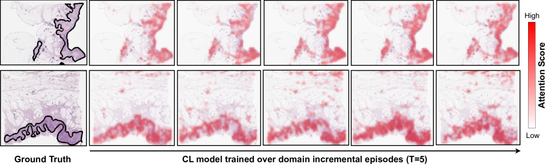
Figure 2: Attention heatmaps for AGLR-CL across domain shifts in MSI prediction. Attentions scores for WSIs from $\mathcal{D}_{1}$ (PAIP-CRC) by the model trained over five CL stages in a2 reflect that past knowledge acquired from $\mathcal{D}_{1}$ is preserved.

Ablation. Table 4 presents an ablation study on attention-based filtering for GMMs training. The results show that, except for sequence a5, GMMs trained with filtered patches consistently outperform those trained on all patch embeddings. For sequence a5, the slight drop may occur due to the high variability of morphological alterations in different TMB outcomes across organs, thus discarding certain patches can hurt data recovery.

5 Conclusion

We proposed AGLR-CL, a buffer-free generative latent replay framework enabling privacy-aware CL for WSI tasks including biomarker screening and molecular status predictions. Instead of maintaining a buffer, AGLR-CL leverages GMMs to synthesize past feature distributions, allowing the model to retain knowledge while adapting to new domains. Results demonstrate that AGLR-CL mitigates CF and achieves state-of-the-art performance in privacy-sensitive CL.

References

- [1] Bhatt, R., Kumari, P., Mahapatra, D., Saddik, A.E., Saini, M.: Characterizing continual learning scenarios and strategies for audio analysis. arXiv preprint arXiv:2407.00465 (2024)
- [2] Cancer Genome Atlas Network: Comprehensive molecular characterization of human colon and rectal cancer. Nature 487(7407), 330–337 (Jul 2012)
- [3] Chen, R.J., Ding, T., Lu, M.Y., Williamson, D.F., Jaume, G., Song, A.H., Chen, B., Zhang, A., Shao, D., Shaban, M., et al.: Towards a general-purpose foundation model for computational pathology. Nature Medicine 30(3), 850–862 (2024)
- [4] Dempster, A.P., Laird, N.M., Rubin, D.B.: Maximum likelihood from incomplete data via the em algorithm. Journal of the royal statistical society: series B (methodological) 39(1), 1–22 (1977)
- [5] Derakhshani, M.M., Najdenkoska, I., van Sonsbeek, T., Zhen, X., Mahapatra, D., Worring, M., Snoek, C.G.: Lifelonger: A benchmark for continual disease classification. In: International Conference on Medical Image Computing and Computer-Assisted Intervention. pp. 314–324. Springer (2022)
- [6] Díaz-Rodríguez, N., Lomonaco, V., Filliat, D., Maltoni, D.: Don’t forget, there is more than forgetting: new metrics for continual learning. arXiv preprint arXiv:1810.13166 (2018)
- [7] Edwards, N.J., Oberti, M., Thangudu, R.R., Cai, S., McGarvey, P.B., Jacob, S., Madhavan, S., Ketchum, K.A.: The CPTAC data portal: A resource for cancer proteomics research. J. Proteome Res. 14(6), 2707–2713 (Jun 2015)
- [8] Fraley, C., Raftery, A.E.: How many clusters? which clustering method? answers via model-based cluster analysis. The computer journal 41(8), 578–588 (1998)
- [9] Huang, Y., Zhao, W., Wang, S., Fu, Y., Jiang, Y., Yu, L.: Conslide: Asynchronous hierarchical interaction transformer with breakup-reorganize rehearsal for continual whole slide image analysis. In: Proceedings of the IEEE/CVF International Conference on Computer Vision. pp. 21349–21360 (2023)
- [10] Ilse, M., Tomczak, J., Welling, M.: Attention-based deep multiple instance learning. In: International conference on machine learning. pp. 2127–2136. PMLR (2018)
- [11] Kim, K., Lee, K., Cho, S., Kang, D.U., Park, S., Kang, Y., Kim, H., Choe, G., Moon, K.C., Lee, K.S., Park, J.H., Hong, C., Nateghi, R., Pourakpour, F., Wang, X., Yang, S., Jahromi, S.A.F., Khani, A., Kim, H.R., Choi, D.H., Han, C.H., Kwak, J.T., Zhang, F., Han, B., Ho, D.J., Kang, G.H., Chun, S.Y., Jeong, W.K., Park, P., Choi, J.: Paip 2020: Microsatellite instability prediction in colorectal cancer. Medical Image Analysis 89, 102886 (Oct 2023). https://doi.org/10.1016/j.media.2023.102886
- [12] Kirkpatrick, J., Pascanu, R., Rabinowitz, N., Veness, J., Desjardins, G., Rusu, A.A., Milan, K., Quan, J., Ramalho, T., Grabska-Barwinska, A., et al.: Overcoming catastrophic forgetting in neural networks. Proceedings of the national academy of sciences 114(13), 3521–3526 (2017)
- [13] Kumari, P., Chauhan, J., Bozorgpour, A., Azad, R., Merhof, D.: Continual learning in medical imaging analysis: A comprehensive review of recent advancements and future prospects. arXiv preprint arXiv:2312.17004 (2023)
- [14] Kumari, P., Choudhary, P., Kujur, V., Atrey, P.K., Saini, M.: Concept drift challenge in multimedia anomaly detection: A case study with facial datasets. Signal Processing: Image Communication p. 117100 (2024)
- [15] Kumari, P., Reisenbüchler, D., Luttner, L., Schaadt, N.S., Feuerhake, F., Merhof, D.: Continual domain incremental learning for privacy-aware digital pathology. In: International Conference on Medical Image Computing and Computer-Assisted Intervention. pp. 34–44. Springer (2024)
- [16] Li, Z., Hoiem, D.: Learning without forgetting. IEEE Transactions on Pattern Analysis and Machine Intelligence 40(12), 2935–2947 (2018). https://doi.org/10.1109/TPAMI.2017.2773081
- [17] Lopez-Paz, D., Ranzato, M.: Gradient episodic memory for continual learning. Advances in neural information processing systems 30 (2017)
- [18] Lu, M.Y., Williamson, D.F., Chen, T.Y., Chen, R.J., Barbieri, M., Mahmood, F.: Data-efficient and weakly supervised computational pathology on whole-slide images. Nature Biomedical Engineering 5(6), 555–570 (2021)
- [19] Prabhu, A., Torr, P.H., Dokania, P.K.: Gdumb: A simple approach that questions our progress in continual learning. In: Computer Vision–ECCV 2020: 16th European Conference, Glasgow, UK, August 23–28, 2020, Proceedings, Part II 16. pp. 524–540. Springer (2020)
- [20] Rolnick, D., Ahuja, A., Schwarz, J., Lillicrap, T., Wayne, G.: Experience replay for continual learning. Advances in Neural Information Processing Systems 32 (2019)
- [21] Wang, X., Du, Y., Yang, S., Zhang, J., Wang, M., Zhang, J., Yang, W., Huang, J., Han, X.: Retccl: Clustering-guided contrastive learning for whole-slide image retrieval. Medical image analysis 83, 102645 (2023)
- [22] Xu, F., Zhu, C., Tang, W., Wang, Y., Zhang, Y., Li, J., Jiang, H., Shi, Z., Liu, J., Jin, M.: Predicting axillary lymph node metastasis in early breast cancer using deep learning on primary tumor biopsy slides. Frontiers in Oncology p. 4133 (2021)
- [23] Xu, H., Usuyama, N., Bagga, J., Zhang, S., Rao, R., Naumann, T., Wong, C., Gero, Z., González, J., Gu, Y., Xu, Y., Wei, M., Wang, W., Ma, S., Wei, F., Yang, J., Li, C., Gao, J., Rosemon, J., Bower, T., Lee, S., Weerasinghe, R., Wright, B.J., Robicsek, A., Piening, B., Bifulco, C., Wang, S., Poon, H.: A whole-slide foundation model for digital pathology from real-world data. Nature (2024)
- [24] Zenke, F., Poole, B., Ganguli, S.: Continual learning through synaptic intelligence. In: International conference on machine learning. pp. 3987–3995. PMLR (2017)
- [25] Zhu, X., Jiang, Z., Wu, K., Shi, J., Zheng, Y.: Lifelong histopathology whole slide image retrieval via distance consistency rehearsal. In: International Conference on Medical Image Computing and Computer-Assisted Intervention. pp. 274–284. Springer (2024)