Learning Advanced Self-Attention for Linear Transformers
in the Singular Value Domain

Abstract

Transformers have demonstrated remarkable performance across diverse domains. The key component of Transformers is self-attention, which learns the relationship between any two tokens in the input sequence. Recent studies have revealed that the self-attention can be understood as a normalized adjacency matrix of a graph. Notably, from the perspective of graph signal processing (GSP), the self-attention can be equivalently defined as a simple graph filter, applying GSP using the value vector as the signal. However, the self-attention is a graph filter defined with only the first order of the polynomial matrix, and acts as a low-pass filter preventing the effective leverage of various frequency information. Consequently, existing self-attention mechanisms are designed in a rather simplified manner. Therefore, we propose a novel method, called Attentive Graph Filter (AGF), interpreting the self-attention as learning the graph filter in the singular value domain from the perspective of graph signal processing for directed graphs with the linear complexity w.r.t. the input length $n$, i.e., $\mathcal{O}(nd^{2})$. In our experiments, we demonstrate that AGF achieves state-of-the-art performance on various tasks, including Long Range Arena benchmark and time series classification.

1 Introduction

Transformers Vaswani et al. (2017) have achieved great success in many fields, including computer vision Touvron et al. (2021a); Liu et al. (2021), time series analysis Li et al. (2019); Wu et al. (2021); Zhou et al. (2021), natural language processing Nangia and Bowman (2018); Maas et al. (2011); Radford et al. (2019); Devlin et al. (2019), and many other works Xiong et al. (2021); Wang et al. (2020); Yu et al. (2024); Kim et al. (2024). Many researchers agree that the self-attention mechanism plays a major role in the powerful performance of Transformers. The self-attention mechanism employs a dot-product operation to calculate the similarity between any two tokens of the input sequence, allowing all other tokens to be attended when updating one token.

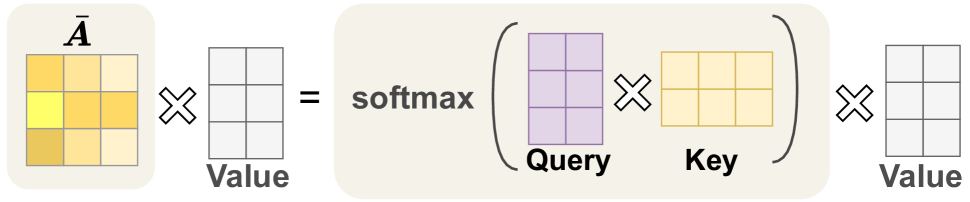
(a) Vanilla self-attention in Transformers

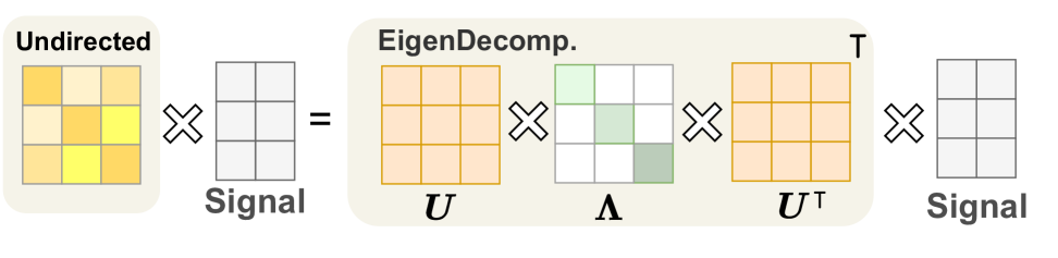
(b) Graph signal processing on undirected graph

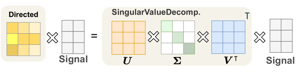
(c) Graph signal processing on directed graph

Figure 1: Illustration of the vanilla self-attention in Transformers and graph signal processing: (a) shows the softmax operation after the dot-product of query and key vectors, followed by the multiplication with the value vector; (b) and (c) show graph signal processing in undirected and directed graphs, respectively. For undirected graphs, the signal is filtered in the eigenvalue domain, while for directed graphs, the signal is filtered in the singular value domain.

Linear Transformers approximate the self-attention.

However, the self-attention requires quadratic complexity over the input length to calculate the cosine similarity between any two tokens. This makes the self-attention difficult to apply to inputs with long lengths. In order to process long sequences, therefore, reducing the complexity of self-attention has become a top-priority goal, leading to the proposal of approximating the self-attention with linear complexity Child et al. (2019); Ravula et al. (2020); Zaheer et al. (2020); Beltagy et al. (2020); Wang et al. (2020); Katharopoulos et al. (2020); Choromanski et al. (2020); Shen et al. (2021); Xiong et al. (2021); Qin et al. (2022); Chen et al. (2023). However, existing self-attention with linear complexity aims to create a matrix that is close to the original self-attention map $\bar{\mathbf{A}}$.

The self-attention is a low-pass filter (see Thm. 1).

The self-attention map is a matrix that represents the relationship between every pair of tokens as scores normalized to probability by softmax. Considering each token as a node and the attention score as an edge weight, self-attention is considered as a normalized adjacency matrix from the perspective of the graph Shi et al. (2022); Wang et al. (2022); Choi et al. (2024). Therefore, the self-attention plays an important role in the message passing scheme by determining which nodes to exchange information with. Given that the self-attention operates as a normalized adjacency matrix, it is intuitively aligned with graph signal processing (GSP) Ortega et al. (2018); Marques et al. (2020); Chien et al. (2021); Defferrard et al. (2016), which employs graph structures to analyze and process signals. Fig. 1 illustrates the self-attention in Transformers and signal filtering in GSP. As depicted in Fig. 1 (a), the original self-attention takes the softmax of the output from the dot product of the query vector and the key vector, and then multiplies it by the value vector. Fig. 1 (b) illustrates a general GSP method that applies the graph Fourier transform to the signal, conducts filtering in the spectral domain, and subsequently restores it to the original signal domain. In GSP, a signals are filtered through the graph filters, which are generally approximated by a matrix polynomial expansion. The self-attention mechanism in Transformers can be viewed as a graph filter $\mathbf{H}$ defined with only the first order of the polynomial matrix, i.e., $\mathbf{H}=\mathbf{\bar{A}}$. Furthermore, since the self-attention is normalized by softmax and functions as a low-pass filter (see Theorem. 1), the high-frequency information in the value vector is attenuated, preventing the effective leverage of various frequency information. Consequently, existing self-attention mechanisms are designed in a rather simplified manner.

Our proposed linear Transformer learns an advanced self-attention (see Thm. 2).

Although the approximation of linear Transformers is successful, what they are doing is simply a low-pass filtering. Therefore, to increase the expressive power of linear Transformers, we propose a more generalized GSP-based self-attention, called Attentive Graph Filter (AGF). We interpret the value vector of Transformers as a signal and redesign the self-attention as a graph filter. However, the existing self-attention mechanism possesses two problems: i) since the self-attention is based on directed graphs, the graph Fourier transform through eigendecomposition is not always guaranteed, and ii) the attention map change for every batch, making it too costly to perform the graph Fourier transform every batch. In order to address the first problem, therefore, we design a self-attention layer based on the GSP process in the singular value domain (see Fig. 1 (c)). The singular value decomposition (SVD) has been used recently for the GSP in directed graphs and can substitute the eigendecomposition Maskey et al. (2023). In order to address the second problem, we directly learn the singular values and vectors instead of explicitly decomposing the self-attention map or any matrix. Since our proposed self-attention layer directly learns in the singular value domain by generating singular vectors and values using a neural network, our proposed method has a linear complexity of $O(nd^{2})$. Therefore, our method efficiently handles inputs with long sequences.

Our contributions can be summarized as follows:

1. We propose an advanced self-attention mechanism based on the perspective of signal processing on directed graphs, called Attentive Graph Filter (AGF), motivated that the self-attention is a simple graph filter and acts as a low pass filter in the singular value domain.

2. AGF learns a sophisticated graph filter directly in the singular value domain with linear complexity w.r.t. input length, which incorporates both low and high-frequency information from hidden representations.

3. The experimental results for time series, long sequence modeling and image domains demonstrate that AGF outperforms existing linear Transformers.

4. As a side contribution, we conduct additional experiments to show that AGF effectively mitigates the over-smoothing problem in deep Transformer models, where the hidden representations of tokens to become indistinguishable from one another.

2 Background

2.1 Self-attention in Transformer

A key operation of Transformers is the self-attention which allows them to learn the relationship among tokens. The self-attention mechanism, denoted as SA: $\mathbb{R}^{n\times d}\rightarrow\mathbb{R}^{n\times d}$, can be expressed as follows:

$$\textrm{SA}(\mathbf{X})=\textrm{softmax}\Big{(}\frac{\mathbf{X}\mathbf{W}_{\textrm{qry}}(\mathbf{X}\mathbf{W}_{\textrm{key}})^{\intercal}}{\sqrt{d}}\Big{)}\mathbf{X}\mathbf{W}_{\textrm{val}}=\bar{\mathbf{A}}\mathbf{X}\mathbf{W}_{\textrm{val}},$$ (1)

where $\mathbf{X}\in\mathbb{R}^{n\times d}$ is the input feature and $\widebar{\mathbf{A}}\in\mathbb{R}^{n\times n}$ is the self-attention matrix. $\mathbf{W}_{\textrm{qry}}\in\mathbb{R}^{d\times d}$, $\mathbf{W}_{\textrm{key}}\in\mathbb{R}^{d\times d}$, and $\mathbf{W}_{\textrm{val}}\in\mathbb{R}^{d\times d}$ are the query, key, and value trainable parameters, respectively, and $d$ is the dimension of token. The self-attention effectively learns the interactions of all token pairs and have shown reliable performance in various tasks.

However, in the case of the existing self-attention, a dot-product is used to calculate the attention score for all token pairs. To construct the self-attention matrix $\widebar{\mathbf{A}}\in\mathbb{R}^{n\times n}$, the matrix multiplication with query and key parameters mainly causes a quadratic complexity of $\mathcal{O}(n^{2}d)$. Therefore, it is not suitable if the length of the input sequence is large. This is one of the major computational bottlenecks in Transformers. For instance, BERT Devlin et al. (2019), one of the state-of-the-art Large Language Model (LLM), needs 16 TPUs for pre-training and 64 TPUs with large models.

2.2 Linear Transformer

To overcome the quadratic computational complexity of the self-attention, efficient Transformer variants have been proposed in recent years. Recent research focuses on reducing the complexity of the self-attention in two streams. The first research line is to replace the softmax operation in the self-attention with other operations. For simplicity, we denote $\textrm{softmax}(\mathbf{X}\mathbf{W}_{qry}(\mathbf{X}\mathbf{W}_{key})^{\intercal})$ as $\textrm{softmax}(\mathbf{Q}\mathbf{K}^{\intercal})$. Wang et al. (2020) introduce projection layers that map value and key vectors to low dimensions. Katharopoulos et al. (2020) interprets softmax as kernel function and replace the similarity function with $\textrm{elu}(\mathbf{x})+1$. Choromanski et al. (2020) approximates the self-attention matrix with random features. Shen et al. (2021) decomposes the $\textrm{softmax}(\mathbf{QK}^{\intercal})$ into $\textrm{softmax}(\mathbf{Q})\textrm{softmax}(\mathbf{K}^{\intercal})$, which allows to calculate $\textrm{softmax}(\mathbf{K}^{\intercal})\mathbf{V}$ first, reducing the complexity from $\mathcal{O}(n^{2}d)$ to $\mathcal{O}(nd^{2})$. Qin et al. (2022) replaces softmax with a linear operator and adopts a cosine-based distance re-weighting mechanism. Xiong et al. (2021) adopts Nyström method by down sampling the queries and keys in the attention matrix. Chen et al. (2023) employs an asymmetric kernel SVD motivated by low-rank property of the self-attention. However, these approaches sacrifice the performance to directly reduce quadratic complexity to linear complexity.

The second research line is to introduce sparsity in the self-attention. Zaheer et al. (2020) introduces a sparse attention mechanism optimized for long document processing, combining local, random, and global attention to reduce computational complexity while maintaining performance. Kitaev et al. (2020) use locality-sensitive hashing and reversible feed forward network for sparse approximation, while requiring to re-implement the gradient back propagation. Beltagy et al. (2020) employ the self-attention on both a local context and a global context to introduce sparsity. Zeng et al. (2021) take a Bernoulli sampling attention mechanism based on locality sensitive hashing. However, since they do not directly reduce the complexity to linear, they also suffer a large performance degradation, while having only limited additional speed-up.

2.3 Graph Convolutional Filter

The graph signal processing (GSP) can be considered as a generalized concept of the discrete signal processing (DSP). In the definition of DSP, the discrete signal with length $n$ is represented by the vector $\mathbf{x}\in\mathbb{R}^{n}$. Then for the signal filter $\mathbf{g}\in\mathbb{R}^{n}$ that transforms $\mathbf{x}$, the convolution operation $\mathbf{x}*\mathbf{g}$ is defined as follows:

$$y_{i}=\sum_{j=1}^{n}\mathbf{x}_{j}\mathbf{g}_{i-j},$$ (2)

where the index $i$ indicates the $i$-th element of each vector. GSP extends DSP to signal samples indexed by nodes of arbitrary graphs. Then we define the shift-invariant graph convolution filters $\mathbf{H}$ with a polynomial of graph shift operator $\mathbf{S}$ as follows:

$$\mathbf{y}=\mathbf{H}\mathbf{x}=\sum_{k=0}^{K}w_{k}\mathbf{S}^{k}\mathbf{x},$$ (3)

where $K$ is the maximum order of polynomial and $w_{k}\in[-\infty,\infty]$ is a coefficient. The graph filter is parameterized as the truncated expansion with the order of $K$. The most commonly used graph shift operators in GSP are adjacency and Laplacian matrices. Note that Eq. (3) applies to any directed or undirected adjacency matrix Ortega et al. (2018); Marques et al. (2020). However, Eq. (3) requires non-trivial matrix power computation. Therefore, we rely on SVD to use the more efficient way in Eq. (5).

3 Proposed Method

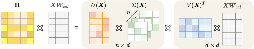
Figure 2: The proposed AGF performs the directed GSP in the singular value domain by learning $U(\mathbf{X})$, $\Sigma(\mathbf{\mathbf{X}})$, and $V(\mathbf{X})$ (cf. Eqs. (8) to (10)). The $n$ different sets of singular values in $\Sigma(\mathbf{X})$ are used for token-specific processing. In other words, $n$ different graph filters are used for $n$ different tokens in order to increase the representation learning capability of AGF.

3.1 Self-attention as a graph filter

The self-attention learns the relationship among all token pairs. From a graph perspective, each token can be interpreted as a graph node and each self-attention score as an edge weight. Therefore, self-attention produces a special case of the normalized adjacency matrix Shi et al. (2022); Wang et al. (2022) and can be analyzed from the perspective of graph signal processing (GSP). In GSP, the low-/high-frequency components of a signal $\mathbf{x}$ are defined using the Discrete Fourier Transform (DFT) $\mathcal{F}$ and its inverse $\mathcal{F}^{-1}$. Let $\bar{\mathbf{x}}=\mathcal{F}\mathbf{x}$ denote the spectrum of $\mathbf{x}$. Then, $\bar{\mathbf{x}}_{\text{lfc}}\in\mathbb{C}^{c}$ contains the $c$ lowest-frequency components of $\bar{\mathbf{x}}$, and $\bar{\mathbf{x}}_{\text{hfc}}\in\mathbb{C}^{n-c}$ contains the remaining higher-frequency components. The low-frequency components (LFC) of $\mathbf{x}$ are given as $\text{LFC}[\mathbf{x}]=\mathcal{F}^{-1}(\bar{\mathbf{x}}_{\text{lfc}})\in\mathbb{R}^{n}$, and the high-frequency components (HFC) are defined as $\text{HFC}[\mathbf{x}]=\mathcal{F}^{-1}(\bar{\mathbf{x}}_{\text{hfc}})\in\mathbb{R}^{n}$. Here, the DFT $\mathcal{F}$ projects $\mathbf{x}$ into the frequency domain, and $\mathcal{F}^{-1}$ reconstructs $\mathbf{x}$ from its spectrum. The Fourier basis $\bm{f}_{j}=[e^{2\pi i(j-1)\cdot 0},e^{2\pi i(j-1)\cdot 1},\dots,e^{2\pi i(j-1)(n-1)}]^{\intercal}/\sqrt{n}$ is used in computing $\mathcal{F}$, where $j$ denotes the $j$-th row. In GSP, the adjacency matrix functions as a low-pass filter, using the edge weights to aggregate information from nodes attenuates the high-frequency information of the nodes. In other words, the self-attention also acts as a low-pass filter within Transformers, and it is theoretically demonstrated below.

Theorem 1 (Self-attention is a low-pass filter).

Let $\mathbf{M}=\textrm{softmax}(\mathbf{Z})$ for any matrix $\mathbf{Z}\in\mathbb{R}^{n\times n}$. Then $\mathbf{M}$ inherently acts as a low pass filter. For all $\mathbf{x}\in\mathbb{R}^{N}$, in other words, $\text{lim}_{t\rightarrow\infty}\|\text{HFC}[\mathbf{M}^{t}(\mathbf{x})]\|_{2}/\|\text{LFC}[\mathbf{M}^{t}(\mathbf{x})]\|_{2}=0$

The proof of Theorem 1 is in Appendix D. As the self-attention is normalized by softmax, the self-attention functions as a low-pass filter. Hence, Transformers are unable to sufficiently leverage a various scale of frequency information, which reduces the expressive power of Transformers.

Inspired by this observation, we redesign a graph filter-based self-attention from the perspective of GSP. As mentioned earlier, since the adjacency matrix can serve as a graph-shift operator, it is reasonable to interpret the self-attention as a graph-shift operator, $\mathbf{S}=\mathbf{\bar{A}}$. Moreover, the self-attention block of the Transformer is equivalent to defining a simple graph filter $\mathbf{H}=\mathbf{\bar{A}}$ and applying GSP to the value vector, treated as a signal. Therefore, in Eq. (3), we can design a more complex graph filter through the polynomial expansion of the self-attention.

Note that when we interpret the self-attention $\mathbf{\bar{A}}$ as a graph, it has the following characteristics: i) The self-attention is an asymmetric directed graph, and ii) all nodes in the graph are connected to each other since the self-attention calculates the relationships among the tokens. Then we can derive that the self-attention is a special case of the symmetrically normalized adjacency (SNA) as $\mathbf{\bar{A}}=\mathbf{D}^{-1}\mathbf{A}$ where $\mathbf{A}$ is an adjacency matrix and $\mathbf{D}$ is a degree matrix of nodes. In particular, SNA is one of the most popular forms for directed GSP Maskey et al. (2023).

3.2 Polynomial graph filter

When approximating the graph filter with a matrix polynomial, $k-1$ matrix multiplications are required to calculate up to the $k$-th order (cf. Eq. (3)), which requires a large computational cost. Therefore, to reduce the computational complexity, we avoid matrix multiplications by directly learning the graph filter in the spectral domain. In the case of an undirected graph, a filter can be learned in the spectral domain by performing the graph Fourier transform through eigendecomposition. In general, however, the eigendecomposition is not guaranteed for directed graphs. The GSP through SVD, therefore, is often used Maskey et al. (2023) if i) a directed graph $\widebar{\mathbf{A}}$ is SNA and ii) its singular values are non-negative and within the unit circle, i.e., $\|\widebar{\mathbf{A}}\|\leq 1$. For $\widebar{\mathbf{A}}$ and its SVD $\widebar{\mathbf{A}}=\mathbf{U}\mathbf{\Sigma}\mathbf{V}^{\intercal}$, an $\alpha$-power of the symmetrically normalized adjacency is defined as:

$$\widebar{\mathbf{A}}^{\alpha}:=\mathbf{U}\mathbf{\Sigma}^{\alpha}\mathbf{V}^{\intercal},$$ (4)

where $\alpha\in\mathbb{R}$ Maskey et al. (2023). Therefore, we can define the graph filter $\mathbf{H}$ as follows:

$$\mathbf{y}=\mathbf{H}\mathbf{x}=g_{\theta}(\mathbf{\bar{A}})\mathbf{x}=\mathbf{U}g_{\theta}(\mathbf{\Sigma})\mathbf{V}^{\intercal}\mathbf{x}=\mathbf{U}(\sum_{k=0}^{K}\theta_{k}\mathbf{\Sigma}^{k})\mathbf{V}^{\intercal}\mathbf{x},$$ (5)

where $\theta\in\mathbb{R}^{n}$ is a vector for singular value coefficients. Therefore, a spectral filter can be defined as a truncated expansion with $K$-th order polynomials. In other words, unlike directly performing the matrix polynomial as in Eq. (3), the computational cost is significantly reduced by $K$ times element-wise multiplying of the singular values, which are represented as a diagonal matrix.

However, the polynomial expansion in Eq. (5) is parameterized with monomial basis, which is unstable in terms of its convergence since the set of bases is non-orthogonal. Therefore, for stable convergence, a filter can be designed using an orthogonal basis. Note that we have the flexibility to apply any basis when using the polynomial expansion for learning graph filters. In this work, we adopt the Jacobi expansion Askey and Wilson (1985), one of the most commonly used polynomial bases. Furthermore, Jacobi basis is a generalized form of classical polynomial bases such as Chebyshev Defferrard et al. (2016) and Legendre McCarthy et al. (1993), offering strong expressiveness in the graph filter design. Detailed formulas are provided in Appendix F. Therefore, we can define the graph polynomial filter as follows:

$$g_{\theta}(\mathbf{\Sigma})=\sum_{k=0}^{K}\theta_{k}T_{k}(\mathbf{\Sigma}),$$ (6)

where $T_{k}(\cdot)$ is a specific polynomial basis of order $k$.

3.3 Attentive Graph Filter

In order to use Eq. (6), however, we need to decompose the adjacency matrix $\widebar{\mathbf{A}}$, which incurs non-trivial computation. Therefore, we propose to directly learn a graph filter in the singular value domain (instead of learning an adjacency matrix, i.e., a self-attention matrix, and decomposing it). Therefore, as shown in Fig. 2, we propose our attentive graph filter (AGF) as follows:

$$\mathrm{AGF}(\mathbf{X}) =\mathbf{HXW}_{\textrm{val}}=U(\mathbf{X})\Sigma(\mathbf{\mathbf{X}})V(\mathbf{X})^{\intercal}\mathbf{X}\mathbf{W}_{\textrm{val}},$$ (7)

$$U(\mathbf{X}) =\rho(\mathbf{X}\mathbf{W}_{U}) \in\mathbb{R}^{n\times d},$$ (8)

$$\Sigma(\mathbf{X}) =\sum_{k=0}^{K}\theta_{k}T_{k}(\mathrm{diag}(\sigma(\mathbf{X}\mathbf{W}_{\Sigma}))) \in\mathbb{R}^{n\times d\times d},$$ (9)

$$V(\mathbf{X})^{\intercal} =\rho((\mathbf{X}\mathbf{W}_{V})^{\intercal}) \in\mathbb{R}^{d\times n},$$ (10)

where $\mathbf{W}_{U},\mathbf{W}_{\Sigma},\mathbf{W}_{V}\in\mathbb{R}^{d\times d}$ are learnable matrices, $\rho$ is a softmax, and $\sigma$ is a sigmoid. Our proposed model does not apply SVD directly on the computed self-attention or other matrices. Instead, the learnable singular values $\sigma(\mathbf{X}\mathbf{W}_{\Sigma})$ and orthogonally regularized singular vectors $U(\mathbf{X})$ and $V(\mathbf{X})$ are generated by neural network. The singular values are then filtered by the graph filter, denoted as $\Sigma(\mathbf{X})$. To ensure that the elements of the singular value matrix are non-negative and within the unit circle, the sigmoid function is applied to the matrix. Moreover, we observe that the softmax of singular vectors enhances the stability of learning.

We construct our graph filter using the generated singular values, leveraging the Jacobi expansion as an orthogonal polynomial basis. If the trainable coefficients $\theta_{k}$ is allowed to take negative values and learned adaptively, the graph filter can pass low/high-frequency components of the value vector. Therefore, AGF functions as a graph filter that leverages various frequency information from the value vector. Furthermore, unlike the adjacency matrix that remains unchanged in GCNs, the self-attention matrix changes with each batch. To enhance the capacity for addressing these dynamics, AGF incorporates a token-specific graph filter, characterized by $n$ different sets of singular values. This allows to leverage the token-specific frequency information in the singular value domain, increasing the capability to handle complex dynamics in hidden representation.

3.4 Objective Function

In the definition of SVD, $U(\mathbf{X})$ is column orthogonal, $V(\mathbf{X})$ is row orthogonal, and $\Sigma(\mathbf{X})$ is a rectangular diagonal matrix with non-negative real numbers. When we train the proposed model, strictly constraining $U(\mathbf{X})$ and $V(\mathbf{X})$ to be orthogonal requires a high computational cost. Instead, we add a regularization on them since these matrices generated by neural network can be trained to be orthogonal as follows:

$$\begin{split}\mathcal{L}_{ortho}=&\frac{1}{n^{2}}\big{(}\|(U(\mathbf{X})^{\intercal}U(\mathbf{X})-\mathbf{I}\|+\|(V(\mathbf{X})V(\mathbf{X})^{\intercal}-\mathbf{I}\|\big{)},\end{split}$$ (11)

where $\mathbf{I}\in\mathbb{R}^{d\times d}$ is an identity matrix. Therefore, our joint learning objective $\mathcal{L}$ is as follows:

$$\mathcal{L}=\mathcal{L}_{transformer}+\gamma\mathcal{L}_{ortho},$$ (12)

where $\mathcal{L}_{transformer}$ is an original objective function for Transformers. The hyperparameters $\gamma$ controls the trade-off between the loss and the regularization.

3.5 Time and Space Complexities of AGF

Since our AGF is based on the concept of SVD, it is not restricted by softmax for calculating attention scores. Therefore, $U(\mathbf{X})$, $\Sigma(\mathbf{X})$, and $V(\mathbf{X})$ generated by neural network can be freely multiplied according to the combination law of matrix multiplication. First, since $\Sigma(\mathbf{X})$ is a diagonal matrix, by performing element-wise multiplication with $U(\mathbf{X})$ and the diagonal elements of $\Sigma(\mathbf{X})$, $(n\times d)$ matrix is calculated with a time complexity of $\mathcal{O}(nd)$. Next, by multiplying $V(\mathbf{X})$ and the value vector, $(d\times d)$ matrix is calculated with a time complexity of $\mathcal{O}(nd^{2})$. Finally, by multiplying the outputs of steps 1 and 2, the final output is $(n\times d)$ matrix with a time complexity of $\mathcal{O}(nd^{2})$. Therefore, the time complexity is $\mathcal{O}(nd^{2})$ and the space complexity is $\mathcal{O}(nd+d^{2})$.

3.6 Properties of AGF

How to use high-frequency information.

In GSP, the characteristics of the graph filter are determined by the learned coefficients $\theta_{k}$ of the signal. These coefficients allow the graph filter to function as a low-pass, high-pass, or combined-pass filter, depending on the specific needs of each task Defferrard et al. (2016); Marques et al. (2020); Chien et al. (2021), demonstrated by following theorem:

Theorem 2 (Adapted from Chien et al. (2021)).

Assume that the graph $G$ is connected. If $\theta_{k}\geq 0$ for $\forall k\in\{0,1,...,K\}$, $\sum_{k=0}^{K}\theta_{k}=1$ and $\exists k^{\prime}>0$ such that $\theta_{k^{\prime}}>0$, then $g_{\theta}(\cdot)$ is a low-pass graph filter. Also, if $\theta_{k}=(-\alpha)^{k}$ , $\alpha\in(0,1)$ and $K$ is large enough, then $g_{\theta}(\cdot)$ is a high-pass graph filter.

The proof is in Appendix E. Theorem 2 indicates that if the coefficient $\theta_{k}$ of a graph filter can have negative values, and learned adaptively, the graph filter will pass low and high frequency signals appropriately. This flexibility is crucial for effectively processing signals with varying frequency components. Similarly, AGF operates as a filter that modulates frequency information in the singular value domain through the generated singular values and singular vectors. This approach enables AGF to dynamically adjust the frequency components of the signal, providing a more tailored and efficient filtering process. Therefore, unlike conventional Transformers, AGF can appropriately incorporate both low and high frequencies for each task, thereby enhancing the expressive power and adaptability of Transformers.

Comparison with existing linear self-attention methods.

We explain that while our AGF addresses the computational inefficiencies inherent in the vanilla self-attention like existing linear self-attention studies, we take a different approach from them. Instead of using explicit SVDs, our AGF reinterprets self-attention through a GSP lens, using the learnable SVD to learn graph filters directly from the spectral domain of directed graphs. Linformer Wang et al. (2020), the most prominent representative of linear self-attention, approximates the vanilla self-attention through dimensionality reduction, and Nyströmformer Xiong et al. (2021), which reduces to linear complexity with a kernel decomposition method, also efficiently approximates the full self-attention matrix with the Nyström method. Singularformer Wu et al. (2023), a closely related approach, uses a parameterized SVD and linearize the calculation of self-attention. However, like existing linear Transformers, it approximates the original self-attention, which is inherently a low-pass filter. Thus, to the best of our knowledge, existing linear self-attention methods focus on approximating the self-attention and reducing it to linear complexity, whereas our AGF approximates a graph filter rather than the self-attention. This allows AGF to use the token-specific graph filter to improve model representation within the singular value domain.

4 Experiments

	EC	FD	HW	HB	JV	PEMS-SF	SRSCP1	SRSCP2	SAD	UWGL	Avg
Transformer	32.7	67.3	32.0	76.1	98.7	82.1	92.2	53.9	98.4	85.6	71.9
LinearTransformer	31.9	67.0	34.7	76.6	99.2	82.1	92.5	56.7	98.0	85.0	72.4
Reformer	31.9	68.6	27.4	77.1	97.8	82.7	90.4	56.7	97.0	85.6	71.5
Longformer	32.3	62.6	39.6	78.0	98.9	83.8	90.1	55.6	94.4	87.5	72.0
Performer	31.2	67.0	32.1	75.6	98.1	80.9	91.5	56.7	98.4	85.3	71.9
YOSO-E	31.2	67.3	30.9	76.5	98.6	85.2	91.1	53.9	98.9	88.4	72.2
Cosformer	32.3	64.8	28.9	77.1	98.3	83.2	91.1	55.0	98.4	85.6	71.5
SOFT	33.5	67.1	34.7	75.6	99.2	80.9	91.8	55.6	98.8	85.0	72.2
Flowformer	33.8	67.6	33.8	77.6	98.9	83.8	92.5	56.1	98.8	86.6	73.0
Primalformer	33.1	67.1	29.6	76.1	98.3	89.6	92.5	57.2	100.0	86.3	73.0
AGF	36.1	69.9	33.5	79.0	99.5	91.3	93.5	58.9	100.0	89.4	75.1

Table 1: Performance comparison on UEA time series classification. Abbreviations are as follows: EthanolConcentration (EC), FaceDetection (FD), HandWriting (HW), HearBeat (HB), JapaneseVowels (JV), PEMS-SF, SelfRegulation SCP1 (SRSCP1), SelfRegulation SCP2 (SRSCP2), SpokenArabicDigits (SAD), and UWaveGesture Library (UWGL).

	ListOps	Text	Retrieval	Image	Pathfinder	Avg
Transformer	37.1	65.0	79.4	38.2	74.2	58.8
Reformer	19.1	64.9	78.6	43.3	69.4	55.1
Performer	18.8	63.8	78.6	37.1	69.9	53.6
Singularformer	18.7	61.8	76.7	35.3	55.8	49.7
Linformer	37.3	55.9	79.4	37.8	67.6	55.6
Nyströmformer	37.2	65.5	79.6	41.6	70.9	59.0
Longformer	37.2	64.6	81.0	39.1	73.0	59.0
YOSO-E	37.3	64.7	81.2	39.8	72.9	59.2
Primalformer	37.3	61.2	77.8	43.0	68.3	57.5
AGF	38.0	64.7	81.4	42.4	74.0	60.1

Table 2: Performance comparison on LRA benchmark

4.1 Time Series Classification

Experimental settings.

To evaluate the performance of AGF, we employ UEA Time Series Classification Archive Bagnall et al. (2018) which is the benchmark on temporal sequences. Strictly following Wu et al. (2022), we report accuracy for 10 multivariate datasets preprocessed according to Zerveas et al. (2021). We adopt 2-layer Transformer as backbone with 512 hidden dimension on 8 heads and 64 embedding dimension of self-attention. The experiments are conducted on 1 GPU of NVIDIA RTX 3090 24GB. The detailed descriptions are in Appendix H.1.

Experimental results.

Table 1 summarizes the test accuracy of AGF and the state-of-the-art linear Transformer models on the UEA time series classification task. We observe that AGF achieves an average accuracy of 75.1, outperforming the vanilla Transformer and other linear Transformers by large margins across various datasets. This performance gap underscores the effectiveness of our approach in leveraging advanced graph filter-based self-attention to enhance the expressive power of Transformers.

4.2 Long Range Arena Benchmark

Experimental settings.

We evaluate AGF on Long Range Arena (LRA) Tay et al. (2020) benchmark under long-sequence scenarios. Following Xiong et al. (2021), we train 2 layer Transformer with 128 hidden dimension, 2 heads, and 64 embedding dimension with mean pooling. The experiments are conducted on 1 GPU of NVIDIA RTX 3090 24GB. The details are in Appendix H.2.

Experimental results.

We report the top-1 test accuracy on LRA benchmark in Table 2. Our modeldemonstrated the highest average performance, achieving a score of 60.1 — an improvement of 1.3 points over the vanilla Transformer. In contrast, SingularFormer, a close approach that parameterizes SVD, only functions as a low-pass filter and thus fails to achieve optimal performance. Compared with YOSO-E, a state-of-the-art linear-complexity Transformer, AGF improves the performance by a substantial margin.

4.3 Sensitivity Analyses

We conduct sensitivity studies on $K$ and $\gamma$. For other sensitivity studies on are reported in Appendix K.

Sensitivity study on $K$.

We test our model by varying $K$ on UEA time series classification, and the results are shown in Table 3. As $K$ increases, the performance improves. However, beyond a certain threshold, increasing $K$ results in saturation and diminished performance. Therefore, choosing an appropriate $K$ has a significant impact on performance.

Sensitivity study on $\gamma$.

Table 4 summarizes the impact of $\gamma$ on LRA benchmark. The optimal level of regularization applied to learnable singular vectors varies depending on the dataset, and we demonstrate that imposing a certain degree of regularization can enhance training stability.

$K$	EC	FD	JV	PEMS-SF	SRSCP1	UWGL
3	32.3	68.2	98.9	86.7	91.1	84.1
4	31.6	68.8	99.5	89.6	92.2	84.1
6	36.1	68.3	98.9	83.8	91.1	84.4
9	30.8	69.9	99.2	83.8	93.5	86.2
10	32.3	67.5	98.9	87.3	91.1	89.4

Table 3: Effect of $K$ on UEA classification

$\gamma$	ListOps	Text	Retrieval	Image	Pathfinder
$1\text{\times}{10}^{-1}$	38.0	64.3	81.4	40.8	73.1
$1\text{\times}{10}^{-2}$	36.9	64.5	79.8	42.4	73.3
$1\text{\times}{10}^{-3}$	37.2	64.7	79.5	42.0	74.0
$1\text{\times}{10}^{-4}$	37.0	64.2	79.4	41.0	74.0

Table 4: Effect of $\gamma$ on LRA benchmark

	ListOps(2K)	Text(4K)	Retrieval(4K)	Image(1K)	Pathfinder(1K)	Avgerage
Transformer	194.5/5.50	694.8/21.24	1333.7/18.72	334.5/5.88	405.5/5.88	592.6/11.44
Nyströmformer	68.3/0.89	52.3/0.48	187.5/1.93	227.9/1.93	232.6/3.29	153.7/1.70
Performer	90.3/1.67	55.9/0.84	230.7/3.34	296.7/3.34	344.8/6.28	203.7/3.09
Reformer	94.1/1.64	58.1/0.82	244.2/3.29	309.1/3.29	370.7/6.09	215.2/3.03
PrimalFormer	56.5/0.69	93.6/1.37	185.3/2.99	142.9/1.39	180.0/1.52	131.7/1.59
AGF	60.8/0.88	48.4/0.51	252.3/3.95	183.3/2.15	209.3/1.89	150.8/1.90

Table 5: Running time (s/1K-steps) and the peak training memory usage (GB) on LRA benchmark

	EC	FD	HW	HB	PEMS-SF	UWGL
$\mathbf{H}_{UV^{\intercal}}$	29.7	66.6	28.2	76.6	87.3	83.8
$\mathbf{H}_{SVD}$	33.1	67.1	27.1	75.1	88.4	85.9
AGF	36.1	69.9	33.5	79.0	91.3	89.4

Table 6: Ablation study on the graph filter

4.4 Empirical Runtime

Table 5 summarize the results of the runtime and peak memory usage during the training phase. AGF consistently improves the efficiency of both time and space complexity compared to the vanilla Transformer. Specifically, for Text dataset, which have extremely long input sequences, the efficiency of AGF stands out even more. When compared with other linear complexity Transformers, our AGF shows comparable efficiency with longer sequences.

4.5 Ablation Studies

We conduct various ablation studies, and the additional results on $T(\cdot)$ and $\rho$ are in Appendix L.

Effect on the graph filter.

To analyze the impact of graph filter, we conduct an ablation study on the following variants: i) $\mathbf{H}_{UV^{\intercal}}$ refers to the graph filters with parameterized singular vectors and the singular values are fixed as one; ii) $\mathbf{H}_{SVD}$ initializes the singular values to one, allowing them to be learnable from $\mathbf{H}_{UV^{\intercal}}$; and iii) AGF refers to the proposed method. Table 6 shows the result of the effect of the graph filter, and in general, these ablation models leads to suboptimal performance. However, AGF processes the generated signal through the graph filter, allowing the model to use various scales of frequency information. The graph filter enhances the capacity of the model, resulting in optimal performance and demonstrating the effectiveness of AGF.

4.6 Additional Experiments on Deep Transformer

Model	ImageNet-100	ImageNet-1K
DeiT-small	80.6	79.8
+ AGF	81.3	80.3

Table 7: Comparison of performance for DeiT-small trained on ImageNet-100 and ImageNet-1K

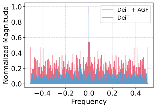
(a) Filter response

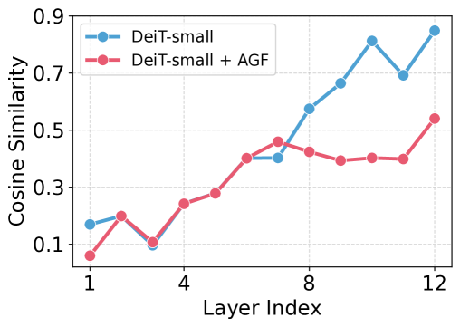
(b) Cosine similarity

Figure 3: Filter response and cosine similarity on ImageNet-1k for DeiT-small and DeiT-small + AGF

Experimental settings.

We conduct additional experiments for image classification task with ImageNet-100 Russakovsky et al. (2015) and ImageNet-1K Deng et al. (2009) datasets and report top-1 accuracy. We adopt DeiT-small as the backbone, and trained from scratch with 300 epochs Touvron et al. (2021b) with 2 GPU of NVIDIA RTX 3090 24GB. The detailed descriptions are in Appendix H.3.

Experimental results.

Table 7 shows the top-1 accuracy on ImageNet-100 and ImageNet-1k. Our AGF effectively learns the representation in deep layers model, which has 12 layers. Notably, plugging AGF improves the performance marginally, from 80.6 to 81.3 trained on ImageNet-100 datasets and from 79.8 to 80.3 on ImageNet-1K.

Analysis on mitigating over-smoothing problem.

Deep Transformers, like GCNs, suffers from over-smoothing problem, where hidden representations become similar and indistinguishable to the last layer Kipf and Welling (2017); Veličković et al. (2018); Oono and Suzuki (2020); Rusch et al. (2023). We previously demonstrated that the self-attention in Transformers acts as a low-pass filter attenuating high-frequency information, which is a major cause of over-smoothing Wang et al. (2022); Shi et al. (2022); Choi et al. (2024). AGF mitigates this issue by effectively leveraging various scale frequency information through directly filtering signals in the singular value domain. Fig. 3 (a) illustrates the frequency information in both the vanilla DeiT (i.e., $\mathbf{H}=\mathbf{\bar{A}}$) and DeiT + AGF (i.e., $\mathbf{H}=\mathbf{U(X)\Sigma(X)\mathbf{V}(X)^{\intercal}}$). Unlike the vanilla model, AGF better captures high-frequency information. Additionally, Fig. 3 (b) shows the cosine similarity among hidden vectors at each layer. While the cosine similarity in DeiT increases to nearly 0.9 as layers deepen, it is moderated to nearly 0.5 in DeiT + AGF. Thus, AGF prevents over-smoothing in deep Transformers by effectively leveraging diverse frequency information.

5 Conclusions

We presented AGF, which interprets the self-attention as learning graph filters in the singular value domain from the perspective of directed graph signal processing. Since the self-attention matrix can be interpreted as a directed graph, we designed a more expressive self-attention using signals directly in the singular value domain. By learning the coefficients for various polynomial bases, AGF uses diverse frequencies. Our experiments showed that AGF outperforms baselines across various tasks, and the training time and GPU usage of AGF are comparable to baseline models with linear complexity. As a side contribution, AGF mitigates the over-smoothing problem in deep Transformers.

Since our comparison scope is focused on linear Transformers, a limitation is the exploration and comparison regarding the recent state-space models Gu et al. (2021); Gu and Dao (2023). Exploring the potential of our method in enhancing state-space models is an intriguing avenue for future work.

Appendix A Reproducibility Statement

In an effort to ensure reproducibility, we report the description of dataset in Appendix G and the best hyperparameters of our experiments in Appendix I.

Appendix B Limitation

The computational benefits of the linear complexity might diminish with extremely large datasets, where the overhead of managing large-scale data can still present challenges. The effectiveness of the approach may vary based on the nature of the input data. Data that do not fit well with the assumptions underlying our graph-based approach might result in sub-optimal performance.

Appendix C Broader Impacts

Our research focuses on improving the efficiency of Transformers by introducing a mechanism to interpret self-attention as a graph filter and reduce it to linear time complexity. Efficient Transformers can have the positive effect of increasing model accessibility for device deployment and training for research purposes. They can also have environmental benefits by reducing carbon footprint. Therefore, our research has no special ethical or social negative implications compared to other key components of deep learning.

Appendix D Proof of Theorem 1

Theorem 1 (Self-attention is a low-pass filter).

Let $\mathbf{M}=\textrm{softmax}(\mathbf{Z})$ for any matrix $\mathbf{Z}\in\mathbb{R}^{n\times n}$. Then $\mathbf{M}$ inherently acts as a low pass filter. For all $\mathbf{x}\in\mathbb{R}^{N}$, in other words, $\text{lim}_{t\rightarrow\infty}\|\text{HFC}[\mathbf{M}^{t}(\mathbf{x})]\|_{2}/\|\text{LFC}[\mathbf{M}^{t}(\mathbf{x})]\|_{2}=0$

Proof.

Given the matrix $\mathbf{M}$ normalized by softmax, $\mathbf{M}$ is a positive matrix and the row-sum of each element in $\mathbf{M}$ is equal to 1. Let the Jordan Canonical Form of $\mathbf{M}$ as $\mathbf{J}$ with the similarity transformation represented by the matrix $P$ as follows:

$$\mathbf{M}=\mathbf{PJP}^{-1},$$ (13)

where $\mathbf{J}$ is block diagonal with each block corresponding to an eigenvalue and its associated Jordan chains. According to the Perron-Frobenius theorem, the largest eigenvalue is real, non-negative and dominant. We denote this eigenvalue as $\lambda_{1}$.

Consider now the repeated application of $\mathbf{M}$:

$$f^{t}(\mathbf{x})=\mathbf{M}^{t}\mathbf{x}=(\mathbf{P}\mathbf{J}\mathbf{P}^{-1})^{t}\mathbf{x}.$$ (14)

By expanding this expression using the binomial theorem and considering the structure of Jordan blocks, we observe that for large $t$, the dominant term will be $\lambda_{1}$. In comparison to the term with $\lambda_{1}$, other terms that involve smaller eigenvalues or higher powers of $t$ in Jordan blocks will become negligible over time.

In the frequency domain, expressing the transformation shows that high-frequency components attenuate faster than the primary low-frequency component. This occurs because the term $\lambda_{1}$ becomes overwhelmingly dominant as $t$ increases, causing other components to diminish.

Thus, within the context of our filter definitions, it becomes evident that:

$$\lim_{t\rightarrow\infty}\frac{||\text{HFC}[f^{t}(\mathbf{x})-\lambda_{1}^{t}\mathbf{v}_{1}]||_{2}}{||\text{LFC}[\lambda_{1}^{t}\mathbf{v}_{1}]||_{2}}=0$$ (15)

Here, $\mathbf{v}_{1}$ is the generalized eigenvector corresponding to $\lambda_{1}$.

This behavior indicates a characteristic of a low-pass filter, reaffirming the low-pass nature of $\mathbf{M}$. Importantly, this is independent of the specific configurations of the input matrices $\mathbf{Z}$. ∎

Appendix E Proof of Theorem 2

Theorem 2.

Assume the graph $G$ is connected. Let $\lambda_{1}\geq\lambda_{2}\geq...\geq\lambda_{n}$ be the singular values of $\mathbf{\bar{A}}$. If $\theta_{k}\geq 0$ for $\forall k\in\{0,1,...,K\}$, $\sum_{k=0}^{K}\theta_{k}=1$ and $\exists k^{\prime}>0$ such that $\theta_{k^{\prime}}>0$, then $\left|g_{\theta}(\lambda_{i})/g_{\theta}(\lambda_{1})\right|<1$ for $\forall i\geq 2$. Also, if $\theta_{k}=(-\alpha)^{k}$ , $\alpha\in(0,1)$ and $K\rightarrow\infty$, then $\left|\text{lim}_{K\rightarrow\infty}g_{\theta}(\lambda_{i})/\text{lim}_{K\rightarrow\infty}g_{\theta}(\lambda_{1})\right|>1$ for $\forall i\geq 2$.

Proof.

For unfiltered case, the singular value ratio is $\left|g_{\theta}(\lambda_{i})/g_{\theta}(\lambda_{1})\right|=1$. Note that $\left|g_{\theta}(\lambda_{i})/g_{\theta}(\lambda_{1})\right|<1$ for $\forall i\geq 2$ implies that after applying the graph filter, the lowest frequency component $\lambda_{1}$ further dominates, which indicates the graph filter $g_{\theta}$ act as a low-pass filter. In contrast $\left|{\text{lim}_{K\rightarrow\infty}g_{\theta}(\lambda_{i})}/{\text{lim}_{K\rightarrow\infty}g_{\theta}(\lambda_{1})}\right|>1$ for $\forall i\geq 2$ indicates the lowest frequency component no longer dominates. This correspond to the high-pass filter case.

For low-pass filter result, from basic spectral analysis Von Luxburg [2007], we know that $\lambda_{1}=1$ and $\left|\lambda_{i}\right|<1$ for $\forall i\geq 2$. By the assumption we know that

$$g_{\theta}(\lambda_{1})=\sum_{k=0}^{K}\theta_{k}=1$$ (16)

Then proving the low-pass filter results is equivalent to show $g_{\theta}(\lambda_{i})<1$ for $\forall i\geq 2$. Since $\theta$ contains non-negative values and for $\forall k\geq 2$, $|\lambda|^{k}<1$ because $|\lambda|<1$, we have:

$$g_{\theta}(\lambda_{i})\leq\sum_{k=0}^{K}\theta_{k}|\lambda^{k}|=\sum_{k=0}^{K}\theta_{k}|\lambda|^{k}\overset{(a)}{\leq}\sum_{k=0}^{K}\theta_{k}=1.$$ (17)

Since by assumption $\sum_{k=0}^{K}\theta_{k}=1$ and $\exists k^{\prime}>0$ such that $\theta_{k^{\prime}}>0$, (a) is a strict inequality $<$. Therefore, the ratio $\left|{g_{\theta}(\lambda_{i})}/{g_{\theta}(\lambda_{1})}\right|<1$ for $\forall i\geq 2$, we prove the low-pass filter result.

For high-pass filter result, it is clarified that

$$\text{lim}_{K\rightarrow\infty}g_{\theta}(\lambda) =\text{lim}_{K\rightarrow\infty}\sum_{k=0}^{K}\theta_{k}\lambda^{k}$$ (18)

$$=\text{lim}_{K\rightarrow\infty}\sum_{k=0}^{K}(-\alpha\lambda)^{k}$$ (19)

$$=\frac{1}{1+\alpha\lambda}$$ (20)

Thus we have:

$$\left|\frac{\text{lim}_{K\rightarrow\infty}g_{\theta}(\lambda_{i})}{\text{lim}_{K\rightarrow\infty}g_{\theta}(\lambda_{1})}\right|=\left|\frac{1+\alpha}{1+\alpha\lambda_{i}}\right|>1$$ (21)

for $\forall i\geq 2$.

Therefore, when the graph filter contains $\theta_{k}=(-\alpha)^{k}$ emphasizes the high-frequency components and acts as a hgih-pass filter.

This proof demonstrates that the characteristic of the grah filter, whether as a low-pass of high-pass filter, directly depends on the sign and values of the coefficients. ∎

Appendix F Jacobi Basis

Jacobi basis $\mathbf{B}_{k}^{a,b}(x)$ is recursively defined as follows:

$$\mathbf{B}_{0}^{a,b}(x)=1,\ \mathbf{B}_{1}^{a,b}(x)=\frac{a-b}{2}+\frac{a+b+2}{2}x.$$ (22)

For $k\geq 2$, it is defined as

$$\mathbf{B}_{k}^{a,b}(x)=(w_{k}x+w_{k}^{\prime})\mathbf{B}_{k-1}^{a,b}(x)-w_{k}^{\prime\prime}\mathbf{B}_{k-2}^{a,b}(x),$$ (23)

where

$$w_{k} =\frac{(2k+a+b)(2k+a+b+1)}{2k(k+a+b)},$$ (24)

$$w_{k}^{\prime} =\frac{(2k+a+b-1)(a^{2}-b^{2})}{2k(k+a+b)(2k+a+b-2)},$$ (25)

$$w_{k}^{\prime\prime} =\frac{(k+a-1)(k+b-1)(2k+a+b)}{k(k+a+b)(2k+a+b-2)},$$ (26)

The Jacobi bases $\mathbf{B}_{k}^{a,b}$ for $k=0,\cdots,j$ are orthogonal with respect to the weight function $(1-x)^{a}(1+x)^{b}$ in the interval $[-1,1]$ with $a,b>-1$. Therefore, we use the Jacobi basis to stabilize the training of the coefficients.

Appendix G Dataset Description

G.1 Long Range Arena Benchmark

Datasets	#Train	#Test	Lengths	#Classes
Listops	96,000	2,000	2K	10
Text	25,000	25,000	4K	2
Retrieval	147,086	17,437	4K	2
Image	45,000	10,000	1K	10
Pathfinder	160,000	20,000	1K	2

Table 8: Statistics of Long Range Arena benchmark datasets

We describe the statistics of Long Range Arena benchmark, including equation calculation (ListOps) Nangia and Bowman [2018], review classification (Text) Maas et al. [2011], document retrieval (Retrieval) Radev et al. [2013], image classification (Image) Krizhevsky et al. [2009], and image spatial dependencies (Pathfinder) Linsley et al. [2018]. Long Range Arena (LRA) is a benchmark to systematically evaluate efficient Transformer models. The statistics of datasets are summarized in Table 8. Also, the descriptions of datasets are as follows:

• ListOps: The consists of summarization operations on a list of single-digit integers written in prefix notation. The entire sequence has a corresponding solution that is also a single-digit integer. Target task is a 10-way balanced classification problem.

• Text: The byte/character-level setup in order to simulate a longer input sequence. This task uses the IMDb reviews dataset, which is a commonly used dataset to benchmark document classification, with a fixed max length of 4K. This is a binary classification task with accuracy.

• Retrieval: To evaluate the ability to encode and store compressed representations that are useful for matching and retrieval, the task is to learn the similarity score between two vectors. This is a binary classification task with accuracy as the metric.

• Image: This task is an image classification task, where the inputs are sequences of pixels which is flatten to a sequence of length as $n^{2}$. CIFAR-10 is used to image classfication.

• Pathfinder: The task evaluates a model to make a binary decision whether two points represented as circles are connected by a path consisting of dashes.

G.2 UEA Time Series Classification

Datasets	#Train	#Test	#Features	Lengths	#Classes
EthanolConcentration	261	263	3	1,751	4
FaceDetection	5,890	3,524	144	62	2
HandWriting	150	850	3	152	26
Heartbeat	204	205	61	405	2
JapaneseVowels	270	370	12	29	9
PEMS-SF	267	173	963	144	7
SelfRegulationSCP1	268	293	6	896	2
SelfRegulationSCP2	200	180	7	1,152	2
SpokenArabicDigits	6,599	2,199	13	93	10
UWaveGestureLibrary	120	320	3	315	8

Table 9: Statistics of UEA time series classification benchmark datasets

We describe the statistics of the UEA time series classification datasets in Table 9.

• EthanolConcentration: A dataset of raw spectra of water-and-ethanol solu- tions in 44 distinct, real whisky bottles.

• FaceDetection: A dataset consisting of MEG recordings and class labels (Face/Scramble)

• HandWriting: A motion dataset taken from a smartwatch while the subject writes 26 letters of the alphabet generated by UCR.

• Heartbeat: Recordings of heart sounds collected from both healthy subjects and pathological patients in clinical or non-clinical settings.

• JapaneseVowels: A dataset where nine Japanese-male speakers were recorded saying the vowels ‘a’ and ‘e’.

• PEMS-SF: A UCI dataset from the California Department of Transportation19 with 15 months worth of daily data from the California Department of Transportation PEMS website.

• SelfRegulationSCP1: A dataset is Ia in BCI II 12: Self-regulation of slow cortical potentials.

• SelfRegulationSCP2: A dataset is Ib in BCI II 12: Self-regulation of slow cortical potentials.

• SpokenArabicDigits: A dataset taken from 44 males and 44 females Arabic native speakers between the ages 18 and 40 to represent ten spoken Arabic digits.

• UWaveGestureLibrary: A set of eight simple gestures generated from accelerometers.

Appendix H Experimental Setting

H.1 UEA Time Series Classification

We compare our model with vanilla Transformer and linear complexity Transformers, including Reformer Kitaev et al. [2020], Linformer Wang et al. [2020], Nyströmformer Xiong et al. [2021], Longformer Beltagy et al. [2020], YOSO-E Zeng et al. [2021], and PirmalFormer Chen et al. [2023]. We grid search the order of polynomial $K$ in {2,3,4,5}, $a$ in {1.0, 1.5, 2.0}, $b$ in {-2.0, -1.5, $\cdots$, 1.5, 2.0}, and $\gamma$ in {$1\text{\times}{10}^{-01}$, $1\text{\times}{10}^{-02}$, $1\text{\times}{10}^{-03}$, $1\text{\times}{10}^{-04}$}.

H.2 Long Range Arena Benchmark

We compare our model with vanilla Transformer and linear complexity Transformers, including LinearTransformer Katharopoulos et al. [2020], Reformer Kitaev et al. [2020], Performer Choromanski et al. [2020], Longformer Beltagy et al. [2020], YOSO-E Zeng et al. [2021], Cosformer Qin et al. [2022], SOFT Lu et al. [2021], Flowformer Wu et al. [2022], and PirmalFormer Chen et al. [2023]. We grid search the order of polynomial $K$ in {2,3,4,5}, $\gamma$ in {$1\text{\times}{10}^{-01}$, $1\text{\times}{10}^{-02}$, $1\text{\times}{10}^{-03}$, $1\text{\times}{10}^{-04}$}, and learning rate $\eta$ in {$1\text{\times}{10}^{-3}$,$5\text{\times}{10}^{-4}$,$1\text{\times}{10}^{-4}$, $5\text{\times}{10}^{-5}$}.

H.3 Vision Transformer

Many recent works do not apply the proposed method to all layers, but adjust the number of layers to apply the proposed method Patro et al. [2023]; Chen et al. [2023]. Therefore, we set the number of applied layers $L$ as a hyperparameter. We conduct experiments with grid search on the order of polynomial $K$ in {3,4}, $\gamma$ in {$1\text{\times}{10}^{-03}$, $1\text{\times}{10}^{-04}$}, and the number of layers $L$ in {1, 3, 6}.

Datasets	$K$	$\gamma$	$a$	$b$
EthanolConcentration	6	0.1	1.5	-1.5
FaceDetection	9	0.1	2.0	0.5
HandWriting	3	0.01	1.0	0.2
Heartbeat	6	0.01	-0.5	-0.5
JapaneseVowels	4	0.01	0.0	0.0
PEMS-SF	5	0.1	1.5	2.0
SelfRegulationSCP1	9	0.1	1.5	2.0
SelfRegulationSCP2	7	0.1	2.0	1.5
SpokenArabicDigits	4	0.1	1.0	0.0
UWaveGestureLibrary	10	0.1	2.0	1.5

Table 10: Best hyperparameters for AGF in UEA time series classification

Datasets	$K$	$\gamma$	$a$	$b$	$\eta$
Text	5	0.001	1.0	1.0	$5\text{\times}{10}^{-05}$
Image	7	0.01	2.0	-1.0	$1\text{\times}{10}^{-3}$
Retrieval	5	0.1	1.0	1.0	$5\text{\times}{10}^{-4}$
ListOps	5	0.1	1.5	1.0	$1\text{\times}{10}^{-3}$
Pathfinder	3	0.0001	1.5	-1.0	$1\text{\times}{10}^{-4}$

Table 11: Best hyperparameters for AGF in Long Range Arena benchmark

Datasets	$K$	$\gamma$	$L$	a	b
ImageNet-100	4	0	1	-0.5	0.0
ImageNet-1k	3	1e-4	6	-0.5	0.0

Table 12: Best hyperparameters for AGF in image classification

Appendix I Best Hyperparameters

Tables 10-12 show the best hyperparameters used in our experiments.

Appendix J Significance Test

We perform a significance test on the UEA time series classification results, as shown in Table 13. Specifically, we use the Wilcoxon signed-rank test, a non-parametric statistical method for comparing differences between two related samples. A $p$-value below 0.05 indicates that the result is statistically significant, suggesting that the observed differences are unlikely to be due to chance.

AGF v.s.	Trans.	Linear.	Re.	Long.	Per.
	0.002	0.010	0.002	0.049	0.002
	YOSO-E	Cos.	SOFT	Flow.	Primal.
	0.002	0.002	0.01	0.004	0.008

Table 13: $p$-value using Wilcoxon signed-rank

Appendix K Sensitivity Studies

In this section, we report the sensitivity studies on UEA time series classification and LRA benchmark for all datasets. Tables 14 and 15 display the comprehensive results of the impact of the polynomial order $K$.

K.1 Effect of the Order of Polynomial $K$

$K$	3	4	5	6	7	8	9	10
EC	32.3	31.6	33.5	36.1	31.9	29.7	30.8	32.3
FD	68.2	68.8	68.1	68.3	68.2	68.3	69.9	67.5
HW	33.5	29.9	33.4	33.2	33.2	32.6	32.5	29.6
HB	77.6	77.6	77.6	79.0	77.6	77.6	77.6	77.6
JV	98.9	99.5	98.9	98.9	99.2	98.9	99.2	98.9
PEMS-SF	86.7	89.6	91.3	83.8	86.1	85.0	83.8	87.3
SRSCP1	91.1	92.2	89.4	91.1	90.8	89.4	93.5	91.1
SRSCP2	55.6	55.6	56.1	56.7	58.9	56.1	56.1	56.1
SAD	100.0	100.0	100.0	100.0	100.0	100.0	100.0	100.0
UWGL	84.1	84.1	86.9	84.4	84.1	85.0	86.2	89.4

Table 14: Effect of $K$ on UEA Time Series classification

$K$	ListOps	Text	Retrieval	Image	Pathfinder
3.0	37.0	64.5	80.6	42.3	74.0
4.0	37.5	64.3	79.7	40.8	74.0
5.0	38.0	64.7	81.4	41.4	72.4
6.0	37.0	64.5	80.6	42.3	71.4
7.0	37.3	63.9	80.0	42.4	72.6

Table 15: Effect of $K$ on Long Range Arena benchmark

We report the sensitivity results for the order of polynomial $K$ on UEA time series classification and LRA benchmark for all datasets. The results are summarized in Tables 14 and  15.

K.2 Effects on the $a$ and $b$ of Jacobi Polynomial

We conduct the senstivity studies on the effect of the parameters $a$ and $b$ in Jacobi polynomial. Tables 16 and 17 summarize the results on UEA time series classification and LRA benchmark for all datasets.

$a$	ListOps	Text	Retrieval	Image	Pathfinder
1.0	36.8	64.7	81.4	41.8	72.5
1.5	38.0	64.3	80.7	41.6	74.0
2.0	36.9	64.2	80.4	42.4	73.4

Table 16: Effect of $a$ on LRA benchmark

$b$	ListOps	Text	Retrieval	Image	Pathfinder
-2.0	37.1	64.1	81.3	40.9	73.4
-1.0	37.6	64.3	80.8	42.4	74.0
1.0	38.0	64.7	81.4	41.6	70.6
2.0	37.0	64.5	81.1	42.3	72.7

Table 17: Effect of $b$ on LRA benchmark

Appendix L Ablation Studies

L.1 Effect of Activation Function $\rho$

	ListOps	Text	Retrieval	Image	Pathfinder
None	17.8	63.4	75.3	41.1	70.6
Sigmoid	17.7	63.1	66.3	40.7	72.3
Tanh	17.8	63.6	77.2	42.2	69.0
Softmax	38.0	64.7	81.4	42.4	74.0

Table 18: Ablation study on $\rho$ in Eqs. (8) and (10)

We conduct an ablation study on the activation function $\rho$ applied to the learnable singular vectors $U(\mathbf{X})$ and $V(\mathbf{X})$. In Table 18, ‘None’ indicates that no activation function is applied to the generated singular vectors, ‘Sigmoid’ and ‘Tanh’ correspond to the use of the sigmoid and hyperbolic tangent functions, respectively, and ‘Softmax’ represents the softmax function used in our proposed model. Consistently, the softmax function demonstrates optimal performance. Since the generated singular vectors serve as the basis for signals in the graph filter, the choice of an appropriate activation function significantly impacts the learning process of the graph filter.

L.2 Effect of Polynomial Type

	EC	FD	HW	HB	JV	PEMS-SF	SRSCP1	SRSCP2	SAD	UWGL	Average
AGF(Monomial)	29.7	67.0	32.4	77.6	98.6	86.7	90.8	55.6	100.0	83.8	72.2
AGF(Jacobi)	36.1	69.9	33.5	79.0	99.5	91.3	93.2	58.9	100.0	89.4	75.1

Table 19: Ablation study on polynomial type

We perform ablation studies on the type of polynomial $T$ and results are shown in Table 18. ‘Monomial’ indicates that we adopt the monomial basis, and ‘Jacobi’ means the Jacobi basis as used in AGF. The Jacobi basis consistently outperforms the Monomial basis, which indicates that the orthogonal basis is stable in terms of convergence and leads to better performance.

L.3 Effect of the Graph Filter

	EC	FD	HW	HB	JV	PEMS-SF	SRSCP1	SRSCP2	SAD	UWGL	Average
$\mathbf{H}_{UV^{\intercal}}$	29.7	66.6	28.2	76.6	98.4	87.3	90.8	56.1	99.9	83.8	71.7
$\mathbf{H}_{SVD}$	33.1	67.1	27.1	75.1	98.4	88.4	89.8	56.1	100.0	85.9	72.1
AGF	36.1	69.9	33.5	79.0	99.5	91.3	93.2	58.9	100.0	89.4	75.1

Table 20: Ablation study on the graph filter

We conduct an ablation study on the signal filtering in main text, especially in subsection 4.5. In this subsection, we show the full results in Table 20. our AGF with appropriate graph signal filtering enhances the self-attention in Transformers, resulting in a significant improvement in average performance.

Appendix M Empirical Runtime

	EC	FD	HW	HB	JV	PEMS-SF	SRSCP1	SRSCP2	SAD	UWGL
Trans.	3.7/13.88	7.3/0.21	0.2/0.44	0.5/1.23	0.3/0.14	0.4/0.41	1.5/4.05	1.5/6.36	3.0/0.22	0.2/0.91
Flow.	2.1/3.75	8.4/0.24	0.4/0.47	0.5/0.95	0.6/0.16	0.4/0.43	1.2/1.96	1.1/2.49	4.8/0.25	0.3/0.78
Primal.	2.1/3.37	10.8/0.22	0.3/0.44	0.5/0.89	0.6/0.15	0.5/0.43	1.3/1.78	1.1/2.16	3.2/0.23	0.2/0.71
AGF	2.7/4.79	10.6/0.32	0.3/0.52	0.5/0.99	0.6/0.18	0.5/0.51	1.7/2.27	1.5/3.31	4.5/0.28	0.3/1.14

Table 21: Comparison of running time (s/epoch) and the peak training memory usage (GB) on UEA time series benchmark

We report the empirical runtime on UEA time series classification and the result is reported in Table 21. It shows comparable efficiency when compared to existing transformers and transformers with linear complexity. The results for LRA benchmark is reported in main text, specifically in Table 5.

References

- Askey and Wilson [1985] Richard Askey and James Arthur Wilson. Some basic hypergeometric orthogonal polynomials that generalize Jacobi polynomials, volume 319. American Mathematical Soc., 1985.
- Bagnall et al. [2018] Anthony Bagnall, Hoang Anh Dau, Jason Lines, Michael Flynn, James Large, Aaron Bostrom, Paul Southam, and Eamonn Keogh. The uea multivariate time series classification archive, 2018. arXiv preprint arXiv:1811.00075, 2018.
- Beltagy et al. [2020] Iz Beltagy, Matthew E Peters, and Arman Cohan. Longformer: The long-document transformer. arXiv preprint arXiv:2004.05150, 2020.
- Chen et al. [2023] Yingyi Chen, Qinghua Tao, Francesco Tonin, and Johan AK Suykens. Primal-attention: Self-attention through asymmetric kernel svd in primal representation. arXiv preprint arXiv:2305.19798, 2023.
- Chien et al. [2021] Eli Chien, Jianhao Peng, Pan Li, and Olgica Milenkovic. Adaptive universal generalized PageRank graph neural network. In ICLR, 2021.
- Child et al. [2019] Rewon Child, Scott Gray, Alec Radford, and Ilya Sutskever. Generating long sequences with sparse transformers. arXiv preprint arXiv:1904.10509, 2019.
- Choi et al. [2024] Jeongwhan Choi, Hyowon Wi, Jayoung Kim, Yehjin Shin, Kookjin Lee, Nathaniel Trask, and Noseong Park. Graph convolutions enrich the self-attention in transformers! Advances in Neural Information Processing Systems, 37:52891–52936, 2024.
- Choromanski et al. [2020] Krzysztof Choromanski, Valerii Likhosherstov, David Dohan, Xingyou Song, Andreea Gane, Tamas Sarlos, Peter Hawkins, Jared Davis, Afroz Mohiuddin, Lukasz Kaiser, et al. Rethinking attention with performers. arXiv preprint arXiv:2009.14794, 2020.
- Defferrard et al. [2016] Michaël Defferrard, Xavier Bresson, and Pierre Vandergheynst. Convolutional neural networks on graphs with fast localized spectral filtering. In NeurIPS, 2016.
- Deng et al. [2009] Jia Deng, Wei Dong, Richard Socher, Li-Jia Li, Kai Li, and Li Fei-Fei. Imagenet: A large-scale hierarchical image database. In 2009 IEEE conference on computer vision and pattern recognition, 2009.
- Devlin et al. [2019] Jacob Devlin, Ming-Wei Chang, Kenton Lee, and Kristina Toutanova. BERT: Pre-training of deep bidirectional transformers for language understanding. In Proceedings of the 2019 Conference of the North American Chapter of the Association for Computational Linguistics: Human Language Technologies, Volume 1 (Long and Short Papers), 2019.
- Gu and Dao [2023] Albert Gu and Tri Dao. Mamba: Linear-time sequence modeling with selective state spaces. arXiv preprint arXiv:2312.00752, 2023.
- Gu et al. [2021] Albert Gu, Karan Goel, and Christopher Ré. Efficiently modeling long sequences with structured state spaces. arXiv preprint arXiv:2111.00396, 2021.
- Katharopoulos et al. [2020] Angelos Katharopoulos, Apoorv Vyas, Nikolaos Pappas, and François Fleuret. Transformers are rnns: Fast autoregressive transformers with linear attention. In ICML. PMLR, 2020.
- Kim et al. [2024] Jayoung Kim, Yehjin Shin, Jeongwhan Choi, Hyowon Wi, and Noseong Park. Polynomial-based self-attention for table representation learning. In International Conference on Machine Learning, pages 24509–24526. PMLR, 2024.
- Kipf and Welling [2017] Thomas N. Kipf and Max Welling. Semi-supervised classification with graph convolutional networks. In ICLR, 2017.
- Kitaev et al. [2020] Nikita Kitaev, Łukasz Kaiser, and Anselm Levskaya. Reformer: The efficient transformer. arXiv preprint arXiv:2001.04451, 2020.
- Krizhevsky et al. [2009] Alex Krizhevsky, Geoffrey Hinton, et al. Learning multiple layers of features from tiny images. 2009.
- Li et al. [2019] Shiyang Li, Xiaoyong Jin, Yao Xuan, Xiyou Zhou, Wenhu Chen, Yu-Xiang Wang, and Xifeng Yan. Enhancing the locality and breaking the memory bottleneck of transformer on time series forecasting. NeurIPS, 2019.
- Linsley et al. [2018] Drew Linsley, Junkyung Kim, Vijay Veerabadran, Charles Windolf, and Thomas Serre. Learning long-range spatial dependencies with horizontal gated recurrent units. NeurIPS, 31, 2018.
- Liu et al. [2021] Ze Liu, Yutong Lin, Yue Cao, Han Hu, Yixuan Wei, Zheng Zhang, Stephen Lin, and Baining Guo. Swin transformer: Hierarchical vision transformer using shifted windows. In ICCV, 2021.
- Lu et al. [2021] Jiachen Lu, Jinghan Yao, Junge Zhang, Xiatian Zhu, Hang Xu, Weiguo Gao, Chunjing Xu, Tao Xiang, and Li Zhang. Soft: Softmax-free transformer with linear complexity. NeurIPS, 34, 2021.
- Maas et al. [2011] Andrew Maas, Raymond E Daly, Peter T Pham, Dan Huang, Andrew Y Ng, and Christopher Potts. Learning word vectors for sentiment analysis. In Proceedings of the annual meeting of the association for computational linguistics: Human language technologies, 2011.
- Marques et al. [2020] Antonio G Marques, Santiago Segarra, and Gonzalo Mateos. Signal processing on directed graphs: The role of edge directionality when processing and learning from network data. IEEE Signal Processing Magazine, 37(6), 2020.
- Maskey et al. [2023] Sohir Maskey, Raffaele Paolino, Aras Bacho, and Gitta Kutyniok. A fractional graph laplacian approach to oversmoothing. In NeurIPS, 2023.
- McCarthy et al. [1993] PC McCarthy, JE Sayre, and BLR Shawyer. Generalized legendre polynomials. Journal of mathematical analysis and applications, 177(2), 1993.
- Nangia and Bowman [2018] Nikita Nangia and Samuel R Bowman. Listops: A diagnostic dataset for latent tree learning. arXiv preprint arXiv:1804.06028, 2018.
- Oono and Suzuki [2020] Kenta Oono and Taiji Suzuki. Graph neural networks exponentially lose expressive power for node classification. In ICLR, 2020.
- Ortega et al. [2018] Antonio Ortega, Pascal Frossard, Jelena Kovačević, José MF Moura, and Pierre Vandergheynst. Graph signal processing: Overview, challenges, and applications. IEEE, 106(5), 2018.
- Patro et al. [2023] Badri N Patro, Vinay P Namboodiri, and Vijay Srinivas Agneeswaran. Spectformer: Frequency and attention is what you need in a vision transformer. arXiv preprint arXiv:2304.06446, 2023.
- Qin et al. [2022] Zhen Qin, Weixuan Sun, Hui Deng, Dongxu Li, Yunshen Wei, Baohong Lv, Junjie Yan, Lingpeng Kong, and Yiran Zhong. cosformer: Rethinking softmax in attention. arXiv preprint arXiv:2202.08791, 2022.
- Radev et al. [2013] Dragomir R Radev, Pradeep Muthukrishnan, Vahed Qazvinian, and Amjad Abu-Jbara. The acl anthology network corpus. Language Resources and Evaluation, 47, 2013.
- Radford et al. [2019] Alec Radford, Jeffrey Wu, Rewon Child, David Luan, Dario Amodei, Ilya Sutskever, et al. Language models are unsupervised multitask learners. OpenAI blog, 1(8):9, 2019.
- Ravula et al. [2020] Anirudh Ravula, Chris Alberti, Joshua Ainslie, Li Yang, Philip Minh Pham, Qifan Wang, Santiago Ontanon, Sumit Kumar Sanghai, Vaclav Cvicek, and Zach Fisher. Etc: Encoding long and structured inputs in transformers. In EMNLP, 2020.
- Rusch et al. [2023] T. Konstantin Rusch, Michael M. Bronstein, and Siddhartha Mishra. A survey on oversmoothing in graph neural networks. arXiv preprint arXiv: Arxiv-2303.10993, 2023.
- Russakovsky et al. [2015] Olga Russakovsky, Jia Deng, Hao Su, Jonathan Krause, Sanjeev Satheesh, Sean Ma, Zhiheng Huang, Andrej Karpathy, Aditya Khosla, Michael Bernstein, et al. Imagenet large scale visual recognition challenge. IJCV, 115, 2015.
- Shen et al. [2021] Zhuoran Shen, Mingyuan Zhang, Haiyu Zhao, Shuai Yi, and Hongsheng Li. Efficient attention: Attention with linear complexities. In ICCV, 2021.
- Shi et al. [2022] Han Shi, Jiahui Gao, Hang Xu, Xiaodan Liang, Zhenguo Li, Lingpeng Kong, Stephen Lee, and James T Kwok. Revisiting over-smoothing in bert from the perspective of graph. In ICLR, 2022.
- Tay et al. [2020] Yi Tay, Mostafa Dehghani, Samira Abnar, Yikang Shen, Dara Bahri, Philip Pham, Jinfeng Rao, Liu Yang, Sebastian Ruder, and Donald Metzler. Long range arena: A benchmark for efficient transformers. arXiv preprint arXiv:2011.04006, 2020.
- Touvron et al. [2021a] Hugo Touvron, Matthieu Cord, Matthijs Douze, Francisco Massa, Alexandre Sablayrolles, and Hervé Jégou. Training data-efficient image transformers & distillation through attention. In ICML, pages 10347–10357. PMLR, 2021.
- Touvron et al. [2021b] Hugo Touvron, Matthieu Cord, Matthijs Douze, Francisco Massa, Alexandre Sablayrolles, and Hervé Jégou. Training data-efficient image transformers & distillation through attention. In ICML. PMLR, 2021.
- Vaswani et al. [2017] Ashish Vaswani, Noam Shazeer, Niki Parmar, Jakob Uszkoreit, Llion Jones, Aidan N Gomez, Łukasz Kaiser, and Illia Polosukhin. Attention is all you need. In NeurIPS, volume 30, 2017.
- Veličković et al. [2018] Petar Veličković, Guillem Cucurull, Arantxa Casanova, Adriana Romero, Pietro Liò, and Yoshua Bengio. Graph Attention Networks. In ICLR, 2018.
- Von Luxburg [2007] Ulrike Von Luxburg. A tutorial on spectral clustering. Statistics and computing, 17, 2007.
- Wang et al. [2020] Sinong Wang, Belinda Z Li, Madian Khabsa, Han Fang, and Hao Ma. Linformer: Self-attention with linear complexity. arXiv preprint arXiv:2006.04768, 2020.
- Wang et al. [2022] Peihao Wang, Wenqing Zheng, Tianlong Chen, and Zhangyang Wang. Anti-oversmoothing in deep vision transformers via the fourier domain analysis: From theory to practice. In ICLR, 2022.
- Wu et al. [2021] Haixu Wu, Jiehui Xu, Jianmin Wang, and Mingsheng Long. Autoformer: Decomposition transformers with auto-correlation for long-term series forecasting. NeurIPS, 34, 2021.
- Wu et al. [2022] Haixu Wu, Jialong Wu, Jiehui Xu, Jianmin Wang, and Mingsheng Long. Flowformer: Linearizing transformers with conservation flows. arXiv preprint arXiv:2202.06258, 2022.
- Wu et al. [2023] Yifan Wu, Shichao Kan, Min Zeng, and Min Li. Singularformer: Learning to decompose self-attention to linearize the complexity of transformer. In IJCAI, pages 4433–4441, 2023.
- Xiong et al. [2021] Yunyang Xiong, Zhanpeng Zeng, Rudrasis Chakraborty, Mingxing Tan, Glenn Fung, Yin Li, and Vikas Singh. Nyströmformer: A nyström-based algorithm for approximating self-attention. In AAAI, volume 35, pages 14138–14148, 2021.
- Yu et al. [2024] Youn-Yeol Yu, Jeongwhan Choi, Woojin Cho, Kookjin Lee, Nayong Kim, Kiseok Chang, ChangSeung Woo, Ilho Kim, SeokWoo Lee, Joon Young Yang, Sooyoung Yoon, and Noseong Park. Learning flexible body collision dynamics with hierarchical contact mesh transformer. In ICLR, 2024.
- Zaheer et al. [2020] Manzil Zaheer, Guru Guruganesh, Kumar Avinava Dubey, Joshua Ainslie, Chris Alberti, Santiago Ontanon, Philip Pham, Anirudh Ravula, Qifan Wang, Li Yang, et al. Big bird: Transformers for longer sequences. NeurIPS, 33:17283–17297, 2020.
- Zeng et al. [2021] Zhanpeng Zeng, Yunyang Xiong, Sathya Ravi, Shailesh Acharya, Glenn M Fung, and Vikas Singh. You only sample (almost) once: Linear cost self-attention via bernoulli sampling. In ICML. PMLR, 2021.
- Zerveas et al. [2021] George Zerveas, Srideepika Jayaraman, Dhaval Patel, Anuradha Bhamidipaty, and Carsten Eickhoff. A transformer-based framework for multivariate time series representation learning. In SIGKDD, 2021.
- Zhou et al. [2021] Haoyi Zhou, Shanghang Zhang, Jieqi Peng, Shuai Zhang, Jianxin Li, Hui Xiong, and Wancai Zhang. Informer: Beyond efficient transformer for long sequence time-series forecasting. In AAAI, volume 35, 2021.