On the role of pairing correlations in calculation of $\beta$-decay half-lives within QRPA formalism

Abstract

In this paper we show that the proton-neutron residual interaction can play an important role in the reliability of calculated $\beta$-decay half-lives. It may also improve the prediction power of the quasiparticle random phase approximation (QRPA) model. We further demonstrate that a reasonable choice of the particle-particle (attractive) and particle-hole force (repulsive) parameters can result in calculated half-lives in very good comparison with the measured ones. Pairing gaps have affect on calculated half-lives which we explore in this paper. We present our half-lives calculation using the proton-neutron QRPA (pn-QRPA) model possessing a multi-shell single-particle deformed space including a schematic interaction for some medium mass neutron-deficient nuclei undergoing $\beta^{+}$/EC decay. Our study shows a better agreement with the available experimental data as compared to former calculations.

1 Introduction

The $\beta$-decay properties are useful tools to better understand the overall picture of nuclear structure [1]. Research on unstable nuclei reveals that $\beta$-decay plays a pivotal role among decay channels [2]. In the field of nuclear astrophysics $\beta$-decay properties of neutron deficient nuclei are involved in astrophysical $rp$-process and are required as input parameters for running numerical simulations [3].

The electron capture (EC) and $\beta^{+}$ decay (at times also referred to as positron decay) is a very important decay mode for neutron deficient nuclei. Various nuclear models have been used in the past to study the properties of $\beta$-decay. Of special mention are those calculations based on gross theory [e.g. [4]], quasiparticle random phase approximation (QRPA) approaches [e.g. [5, 6, 7, 8, 9, 10, 11, 12, 13, 2]] and shell model [e.g. [14]]. The gross theory adopts a statistical approach to get an estimate of the $\beta$-decay properties. On the other hand, the shell model and QRPA approaches are microscopic in nature. Usage of shell model has the obvious constraint of number of basis states which creeps in as soon as we start to study heavy nuclei. Shell model results may be accurate only for light cases [2]. The QRPA approach leads to precise and schematic information about $\beta$-decay properties [8]. Using this method one can reproduce available experimental data for $\beta$-decay half-lives in a reliable and efficient manner. Previously the finite-range droplet model (FRDM) and folded-Yukawa single-particle potential was used to study nuclear properties of around 9000 nuclei ranging from ¹⁶O to ³³⁹136 using the QRPA approach [15]. In past research it was reported that $\beta$-decay half-lives were significantly affected by the proton-neutron pairing interaction [16, 8, 2].

In this paper we calculate and analyze the half-lives of $\beta^{+}$/EC decay for even-even medium mass neutron deficient nuclei with atomic number in the range $Z=24-34$ far from $\beta$-stability line. We perform our calculation using a proton-neutron QRPA (pn-QRPA) base model in a multi-shell single-particle deformed space with schematic and separable Gamow-Teller (GT) potential. We show that a reasonable choice of the particle-particle ($pp$) and particle-hole ($ph$) GT strength parameters (see next section for further explanation) may lead to improved prediction power and reliable calculation of $\beta^{+}$/EC decay half-lives. The calculated half-lives are later compared with measured data [17], FRDM [15] and the recent extended QRPA (EQRPA) calculations [2].

This paper is drafted in following manner. In Sec. 2 we explain our base model (pn-QRPA) and admit necessary formalism for half-life calculation within the framework of deformed pn-QRPA approach. Results and discussion are presented in Section 3. Conclusions and summary are given in Section 4.

2 FORMALISM

The role of residual interaction becomes important as the number of nucleons outside the closed major shell increases. Of special mention is the short-range part of the residual interaction which manifest itself as pairing correlations between the nucleons. This phenomenon is commonly referred to as nucleon pairing. This correlation lowers their total energy by an amount $2\Delta$ (where $\Delta$ is the pairing gap).

For our present study we employ the pn-QRPA model in a deformed space using the Nilsson+BCS formalism. We further incorporate multi-shell single-particle states and include a schematic interaction [5, 6]. See also Ref. [18]. Using this base model we calculated $\beta$-decay half-lives for neutron deficient even-even nuclei possessing neutron number $N$ in the range of 18 to 36.

We started with a spherical basis $(a^{\dagger}_{jk},a_{jk})$, possessing $j$ as its total angular momentum and $k$ as the associated z-component. This basis was later transformed to a deformed (axial-symmetric) basis $(d^{\dagger}_{k\alpha},d_{k\alpha})$ using the transformation equation

$$d^{\dagger}_{k\alpha}=\Sigma_{j}K^{k\alpha}_{j}a^{\dagger}_{jk}.$$ (1)

In Eq. 1 $K$ stands for matrix of transformation obtained from set of Nilsson eigenfunctions, and $\alpha$ (represents additional quantum except $k$) which specify the Nilsson eigenstates. We employed the BCS calculation for neutron and proton systems independently. We took a constant pairing force possessing strength of $V$($V_{n}$, $V_{p}$ for neutrons and protons, respectively),

$$\begin{split}F^{pair}=-V\sum_{jkj^{{}^{\prime}}k^{{}^{\prime}}}(-1)^{l+j-k}a^{\dagger}_{jk}a^{\dagger}_{j-k}(-1)^{l^{{}^{\prime}}+j^{{}^{\prime}}-k^{{}^{\prime}}}\\ a_{j^{{}^{\prime}}-k}a_{j^{{}^{\prime}}k^{{}^{\prime}}},\end{split}$$ (2)

where the sum over $k$ and $k^{{}^{\prime}}$ was limited to $k$, $k^{{}^{\prime}}$ $>$ 0 and $l$ stands for orbital angular momentum. The BCS calculation provides occupation amplitudes $u_{k\alpha}$, $v_{k\alpha}$ (which fulfills $u^{2}_{k\alpha}$+$v^{2}_{k\alpha}$=1) and quasiparticle (q.p.) energies $\varepsilon_{k\alpha}$. It is to be noted that the pairing gaps ($\Delta$) were determined empirically in our calculation and is discussed towards the end of this section. Later we added a q.p. basis $(c^{\dagger}_{k\alpha},c_{k\alpha})$ by introducing a Bogoliubov transformation

$$c^{\dagger}_{k\alpha}=u_{k\alpha}d^{\dagger}_{k\alpha}-v_{k\alpha}d_{\bar{k}\alpha}\\ c^{\dagger}_{\bar{k}\alpha}=u_{k\alpha}d^{\dagger}_{\bar{k}\alpha}+v_{k\alpha}d_{k\alpha}.$$ (3)

Here $\bar{k}$ is the time inverted state of $k$ and $c/c^{\dagger}$ stands for the q.p. annihilation/creation operators which eventually entered our RPA equation. Creation operators of QRPA phonons was introduced using the relation

$$C^{\dagger}_{\omega}(\mu)=\sum_{pn}[X^{pn}_{\omega}(\mu)c^{\dagger}_{p}c^{\dagger}_{n}-Y^{pn}_{\omega}(\mu)c_{n}c_{\overline{p}}].$$ (4)

Indices $n$ and $p$ in Eq. 4 stand for $m_{n}\alpha_{n}$ and $m_{p}\alpha_{p}$, respectively, and distinguish between neutron and proton single-(quasi)-particle states. $X^{pn}_{\omega}$ and $Y^{pn}_{\omega}$ are amplitudes for forward and backward-going, respectively. They are the eigenfunctions for the RPA matrix equation. $\omega$ represents the corresponding energy eigenvalues of the eigenstates.

We consider the $ph$ Gamow-Teller (GT) force for RPA calculation using the relation

$$F^{ph}=+2\chi\sum^{1}_{\mu=-1}(-1)^{\mu}Y_{\mu}Y^{\dagger}_{-\mu}\\$$ (5)

$$Y_{\mu}=\sum_{j_{p}m_{p}j_{n}m_{n}}<j_{p}m_{p}\mid\tau_{-}\sigma_{\mu}\mid j_{n}m_{n}>c^{\dagger}_{j_{p}m_{p}}c_{j_{n}m_{n}}.$$ (6)

The corresponding $pp$ GT force was calculated using

$$F^{pp}=-2\kappa\sum^{1}_{\mu=-1}(-1)^{\mu}Z_{\mu}^{\dagger}Z_{-\mu}.$$ (7)

with

$$\begin{split}Z_{\mu}^{+}=\sum_{j_{p}m_{p}j_{n}m_{n}}<j_{n}m_{n}|(\tau_{-}\sigma_{\mu})^{+}|j_{p}m_{p}>\\ (-1)^{l_{n}+j_{n}-m_{n}}c_{j_{p}m_{p}}^{+}c_{j_{n}-m_{n}}^{+},\end{split}$$ (8)

In Eqs. 6 and  8, $\tau_{\pm}$ is the isospin raising (lowering) operator. The $\tau_{+}$ ($\tau_{-}$) operator transforms a proton (neutron) to a neutron (proton), $\sigma$ is the Pauli matrix. The $pp$ and $ph$ forces were characterized by interaction constants $\kappa$ and $\chi$, respectively. All remaining symbols have their usual meanings.

The construction of low-lying excited states for odd-A nuclei is done using the following recipe in our model:
(1) By exciting odd numbers of neutron from the ground state to high (excited state) energy states.
(2) By three-neutron states, corresponding to excitation of a neutron,
(3) By excitation of a proton, corresponding to one neutron and two protons states.
The quasiparticle states in an even proton and odd neutron nucleus can be obtained from Eqs. 9 and 10 by the interchange of neutron and proton states ($\eta\longleftrightarrow\pi$) and the annihilation (creation) operators of QRPA phonons ($A^{+}_{\omega}(-\mu)\longleftrightarrow A^{+}_{\omega}(\mu)$).
The quasiparticles transition from lower to higher energy levels for odd-proton and even-neutron state is attainable.

$$\begin{split}\mid{\pi_{1}\pi_{2}\pi_{3corr}}\rangle=\alpha^{+}_{\pi_{1}}\alpha^{+}_{\pi_{2}}\alpha^{+}_{\pi_{3}}|{-}\rangle+\\ \dfrac{1}{2}\sum\limits_{\pi^{\prime}_{1}\pi^{\prime}_{2}\eta^{\prime}\omega}\alpha^{+}_{\pi^{\prime}_{1}}\alpha^{+}_{\pi^{\prime}_{2}}\alpha^{+}_{\eta^{\prime}}A^{+}_{\omega}(\mu)|{-}\rangle\\ \langle{-}|[\alpha^{+}_{\pi^{\prime}_{1}}\alpha^{+}_{\pi^{\prime}_{2}}\alpha^{+}_{\eta^{\prime}}A^{+}_{\omega}(\mu)]^{+}H\\ \alpha^{+}_{\pi_{1}}\alpha^{+}_{\pi_{2}}\alpha^{+}_{\pi 3}|{-}\rangle E_{\pi_{1}\pi_{2}\pi_{3}}(\pi^{\prime}_{1}\pi^{\prime}_{2}\eta^{\prime},\omega),\end{split}$$ (9)

here ’$H$’ stands for the Hamiltonian obtained from separable particle-hole (ph) and particle-particle (pp) forces by the Bogoliubov transformation playing vital role for phonon-quasiparticle coupling. The sum is taken over all phonons and quasiparticle proton (neutron) states, satisfying $m_{\pi}-m_{\eta}=\mu$. The symbols $\pi$ and $\eta$ indicate proton and neutron states, respectively.

$$\begin{split}|{\pi_{1}\eta_{1}\eta_{2corr}}\rangle=\alpha^{+}_{\pi_{1}}\alpha^{+}_{\eta_{1}}\alpha^{+}_{\eta_{2}}|{-}\rangle+\\ \dfrac{1}{2}\sum\limits_{\pi^{\prime}_{1}\pi^{\prime}_{2}\eta^{\prime}\omega}\alpha^{+}_{\pi^{\prime}_{1}}\alpha^{+}_{\pi^{\prime}_{2}}\alpha^{+}_{\eta^{\prime}}A^{+}_{\omega}(-\mu)|{-}\rangle\\ \langle{-}|[\alpha^{+}_{\pi^{\prime}_{1}}\alpha^{+}_{\pi^{\prime}_{2}}\alpha^{+}_{\eta^{\prime}}A^{+}_{\omega}(-\mu)]^{+}\\ H\alpha^{+}_{\pi_{1}}\alpha^{+}_{\eta_{1}}\alpha^{+}_{\eta_{2}}|{-}\rangle E_{\pi_{1}\eta_{1}\eta_{2}}(\pi^{\prime}_{1}\pi^{\prime}_{2}\eta^{\prime},\omega)+\dfrac{1}{6}\\ \sum\limits_{\eta^{\prime}_{1}\eta^{\prime}_{2}\eta^{\prime}_{3}\omega}\alpha^{+}_{\eta^{\prime}_{1}}\alpha^{+}_{\eta^{\prime}_{2}}\alpha^{+}_{\eta^{\prime}_{3}}A^{+}_{\omega}(\mu)\\ |{-}\rangle\langle{-}|[\alpha^{+}_{\eta^{\prime}_{1}}\alpha^{+}_{\eta^{\prime}_{2}}\alpha^{+}_{\eta^{\prime}_{3}}A^{+}_{\omega}(\mu)]^{+}\\ H\alpha^{+}_{\pi_{1}}\alpha^{+}_{\eta_{1}}\alpha^{+}_{\eta_{2}}|{-}\rangle E_{\pi_{1}\eta_{1}\eta_{2}}(\eta^{\prime}_{1}\eta^{\prime}_{2}\eta^{\prime}_{3},\omega),\end{split}$$ (10)

with the energy denominator of first order perturbation,

$$E_{abcd}(def,\omega)=\dfrac{1}{(\epsilon_{a}+\epsilon_{b}+\epsilon_{c})-(\epsilon_{d}+\epsilon_{e}+\epsilon_{f}+\omega)}.$$ (11)

The formulae for multi quasi particle transitions and their reduction to correlated one quasi particle state are given as:

$$\begin{split}\langle{\pi^{f}_{1}\pi^{f}_{2}\eta^{f}_{1corr}}|t_{\pm}\sigma_{-\mu}|{\pi^{i}_{1}\pi^{i}_{2}\pi^{i}_{3corr}}\rangle=\\ \delta(\pi^{f}_{1},\pi^{i}_{2})\delta(\pi^{f}_{2},\pi^{i}_{3})\langle{\eta^{f}_{1corr}}|t_{\pm}\sigma_{-\mu}|{\pi^{i}_{1corr}}\rangle\\ -\delta(\pi^{f}_{1},\pi^{i}_{1})\delta(\pi^{f}_{2},\pi^{i}_{3})\langle{\eta^{f}_{\eta 1}}|t_{\pm}\sigma_{-\mu}|{\pi^{i}_{2corr}}\rangle\\ +\delta(\pi^{f}_{1},\pi^{i}_{1})\delta(\pi^{f}_{2},\pi^{i}_{2})\langle{\eta^{f}_{\eta 1}}|t_{\pm}\sigma_{-\mu}|{\pi^{i}_{3corr}}\rangle,\end{split}$$ (12)

$$\begin{split}\langle{\pi^{f}_{1}\pi^{f}_{2}\eta^{f}_{1corr}}|t_{\pm}\sigma_{\mu}|{\pi^{i}_{1}\pi^{i}_{2}\pi^{i}_{2corr}}\rangle=\\ \delta(\eta^{f}_{1},\eta^{i}_{2})[\delta(\pi^{f}_{1},\pi^{i}_{1})\langle{\pi^{f}_{2corr}}|t_{\pm}\sigma_{\mu}|{\eta^{i}_{1corr}}\rangle\\ -\delta(\pi^{f}_{2},\pi^{i}_{1})\langle{\pi^{f}_{corr1}}|t_{\pm}\sigma_{\mu}|{\eta^{i}_{1corr}}\rangle]\\ -\delta(\eta^{f}_{1},\eta^{i}_{1})[\delta(\pi^{f}_{1},\pi^{i}_{1})\langle{\pi^{f}_{2corr}}|t_{\pm}\sigma_{\mu}|{\eta^{i}_{2corr}}\rangle\\ -\delta(\pi^{f}_{2},\pi^{i}_{1})\langle{\pi^{f}_{1corr}}|t_{\pm}\sigma_{\mu}|{\eta^{i}_{2corr}}\rangle],\end{split}$$ (13)

$$\begin{split}\langle{\eta^{f}_{1}\eta^{f}_{2}\eta^{f}_{3corr}}|t_{\pm}\sigma_{-\mu}|{\pi^{i}_{1}\eta^{i}_{1}\eta^{i}_{2corr}}\rangle=\\ \delta(\eta^{f}_{2},\eta^{i}_{1})\delta(\eta^{f}_{3},\eta^{i}_{2})\langle{\eta^{f}_{1corr}}|t_{\pm}\sigma_{-\mu}|{\pi^{i}_{1corr}}\rangle\\ -\delta(\eta^{f}_{1},\eta^{i}_{1})\delta(\eta^{f}_{3},\eta^{i}_{2})\langle{\eta^{f}_{2corr}}|t_{\pm}\sigma_{-\mu}|{\pi^{i}_{1corr}}\rangle\\ +\delta(\eta^{f}_{1},\eta^{i}_{1})\delta(\eta^{f}_{2},\eta^{i}_{2})\langle{\eta^{f}_{3corr}}|t_{\pm}\sigma_{-\mu}|{\pi^{i}_{1corr}}\rangle.\end{split}$$ (14)

For odd-odd nuclei the quasiparticle transformation is expressed by using two quasiparticle states of proton and neutron pair states and four quasiparticle states of two nucleons. Similarly in this case, transition amplitudes for the quasiparticle states are reduced into the correlated one quasiparticle state and given as

$$\begin{split}\langle{\pi^{f}_{1}\pi^{f}_{2corr}}|t_{\pm}\sigma_{\mu}|{\pi^{i}\eta^{i}_{corr}}\rangle=\delta(\pi^{f}_{1},\pi^{i})\langle{\pi^{f}_{2{corr}}}|t_{\pm}\sigma_{\mu}|{\eta^{i}_{corr}}\rangle\\ -\delta(\pi^{f}_{2},\pi^{i})\langle{\pi^{f}_{1{corr}}}|t_{\pm}\sigma_{\mu}|{\eta^{i}_{corr}}\rangle,\end{split}$$ (15)

$$\begin{split}\langle{\eta^{f}_{1}\eta^{f}_{2corr}}|t_{\pm}\sigma_{-\mu}|{\pi^{i}n^{i}_{corr}}\rangle=\delta(\eta^{f}_{2},\eta^{i})\langle{\eta^{f}_{1corr}}|t_{\pm}\sigma_{-\mu}|{\pi^{i}_{corr}}\rangle\\ -\delta(\eta^{f}_{1},\eta^{i})\langle{\eta^{f}_{2corr}}|t_{\pm}\sigma_{-\mu}|{\pi^{i}_{corr}}\rangle.\end{split}$$ (16)

The four quasiparticle states are simplified as following

$$\begin{split}\langle{\pi^{f}_{1}\pi^{f}_{2}\eta^{f}_{1}\eta^{f}_{2corr}}|t_{\pm}\sigma_{-\mu}|{\pi^{i}_{1}\pi^{i}_{2}\pi^{i}_{3}\eta^{i}_{1corr}}\rangle=\\ \delta(\eta^{f}_{2},\eta^{i}_{1})[\delta(\pi^{f}_{1},\pi^{i}_{2})\delta(\pi^{f}_{2},\pi^{i}_{3})\langle{\eta^{f}_{1corr}}|t_{\pm}\sigma_{-\mu}|{\pi^{i}_{1corr}}\rangle\\ -\delta(\pi^{f}_{1},\pi^{i}_{1})\delta(\pi^{f}_{2},\pi^{i}_{3})\langle{\eta^{f}_{1corr}}|t_{\pm}\sigma_{-\mu}|{\pi^{i}_{2corr}}\rangle\\ +\delta(\pi^{f}_{1},\pi^{i}_{1})\delta(\pi^{f}_{2},\pi^{i}_{2})\langle{\eta^{f}_{1corr}}|t_{\pm}\sigma_{-\mu}|{\pi^{i}_{3corr}}\rangle]\\ -\delta(\eta^{f}_{1},\eta^{i}_{1})[\delta(\pi^{f}_{1},\pi^{i}_{2})\delta(\pi^{f}_{2},\pi^{i}_{3})\langle{\eta^{f}_{2corr}}|t_{\pm}\sigma_{-\mu}|{\pi^{i}_{1corr}}\rangle\\ -\delta(\pi^{f}_{1},\pi^{i}_{1})\delta(\pi^{f}_{2},\pi^{i}_{3})\langle{\eta^{f}_{2corr}}|t_{\pm}\sigma_{-\mu}|{\pi^{i}_{2corr}}\rangle\\ +\delta(\pi^{f}_{1},\pi^{i}_{1})\delta(\pi^{f}_{2},\pi^{i}_{2})\langle{\eta^{f}_{2corr}}|t_{\pm}\sigma_{-\mu}|{\pi^{i}_{3corr}}\rangle],\end{split}$$ (17)

$$\begin{split}\langle{\pi^{f}_{1}\pi^{f}_{2}\pi^{f}_{3}\pi^{f}_{4corr}}|t_{\pm}\sigma_{\mu}|{\pi^{i}_{1}\pi^{i}_{2}\pi^{i}_{3}\eta^{i}_{1corr}}\rangle=\\ -\delta(\pi^{f}_{2},\pi^{i}_{1})\delta(\pi^{f}_{3},\pi^{i}_{2})\delta(\pi^{f}_{4},\pi^{i}_{3})\langle{\pi^{f}_{1corr}}|t_{\pm}\sigma_{\mu}|{\eta^{i}_{1corr}}\rangle\\ +\delta(\pi^{f}_{1},\pi^{i}_{1})\delta(\pi^{f}_{3},\pi^{i}_{2})\delta(\pi^{f}_{4},\pi^{i}_{3})\langle{\pi^{f}_{2corr}}|t_{\pm}\sigma_{\mu}|{\eta^{i}_{1corr}}\rangle\\ -\delta(\pi^{f}_{1},\pi^{i}_{1})\delta(\pi^{f}_{2},\pi^{i}_{2})\delta(\pi^{f}_{4},\pi^{i}_{3})\langle{\pi^{f}_{3corr}}|t_{\pm}\sigma_{\mu}|{\eta^{i}_{1corr}}\rangle\\ +\delta(\pi^{f}_{1},\pi^{i}_{1})\delta(\pi^{f}_{2},\pi^{i}_{2})\delta(\pi^{f}_{3},\pi^{i}_{3})\langle{\pi^{f}_{4corr}}|t_{\pm}\sigma_{\mu}|{\pi^{i}_{1corr}}\rangle,\end{split}$$ (18)

$$\begin{split}\langle{\pi^{f}_{1}\pi^{f}_{2}\eta^{f}_{1}\eta^{f}_{2corr}}|t_{\pm}\sigma_{\mu}|{\pi^{i}_{1}\eta^{i}_{1}\eta^{i}_{2}\eta^{i}_{3corr}}\rangle=\\ \delta(\pi^{f}_{1},\pi^{i}_{1})[\delta(\eta^{f}_{1},\eta^{i}_{2})\delta(\eta^{f}_{2},\eta^{i}_{3})\langle{\pi^{f}_{2corr}}|t_{\pm}\sigma_{\mu}|{\eta^{i}_{1corr}}\rangle\\ -\delta(\eta^{f}_{1},\eta^{i}_{1})\delta(\eta^{f}_{2},\eta^{i}_{3})\langle{\pi^{f}_{2corr}}|t_{\pm}\sigma_{\mu}|{\eta^{i}_{2corr}}\rangle\\ +\delta(\eta^{f}_{1},\eta^{i}_{1})\delta(\eta^{f}_{2},\eta^{i}_{2})\langle{\pi^{f}_{2corr}}|t_{\pm}\sigma_{\mu}|{\eta^{i}_{3corr}}\rangle]\\ -\delta(\pi^{f}_{2},\pi^{i}_{1})[\delta(\eta^{f}_{1},\eta^{i}_{2})\delta(\eta^{f}_{2},\eta^{i}_{3})\langle{\pi^{f}_{1corr}}|t_{\pm}\sigma_{\mu}|{\eta^{i}_{1corr}}\rangle\\ -\delta(\eta^{f}_{1},\eta^{i}_{1})\delta(\eta^{f}_{2},\eta^{i}_{3})\langle{\pi^{f}_{1corr}}|t_{\pm}\sigma_{\mu}|{\eta^{i}_{2corr}}\rangle\\ +\delta(\eta^{f}_{1},\eta^{i}_{1})\delta(\eta^{f}_{2},\eta^{i}_{2})\langle{\pi^{f}_{1corr}}|t_{\pm}\sigma_{\mu}|{\eta^{i}_{3corr}}\rangle],\end{split}$$ (19)

$$\begin{split}\langle{\eta^{f}_{1}\eta^{f}_{2}\eta^{f}_{3}\eta^{f}_{4corr}}|t_{\pm}\sigma_{-\mu}|{\pi^{i}_{1}\eta^{i}_{1}\eta^{i}_{2}\eta^{i}_{3corr}}\rangle=\\ +\delta(\eta^{f}_{2},\pi^{i}_{1})\delta(\eta^{f}_{3},\eta^{i}_{2})\delta(\eta^{f}_{4},\eta^{i}_{3})\langle{\eta^{f}_{1corr}}|t_{-\pm}\sigma_{\mu}|{\pi^{i}_{1corr}}\rangle\\ -\delta(\eta^{f}_{1},\eta^{i}_{1})\delta(\eta^{f}_{3},\eta^{i}_{2})\delta(\eta^{f}_{4},\eta^{i}_{3})\langle{\eta^{f}_{2corr}}|t_{\pm}\sigma_{-\mu}|{\pi^{i}_{1corr}}\rangle\\ +\delta(\eta^{f}_{1},\eta^{i}_{1})\delta(\eta^{f}_{2},\eta^{i}_{2})\delta(\eta^{f}_{4},\eta^{i}_{3})\langle{\eta^{f}_{3corr}}|t_{\pm}\sigma_{-\mu}|{\pi^{i}_{1corr}}\rangle\\ -\delta(\eta^{f}_{1},\eta^{i}_{1})\delta(\eta^{f}_{2},\eta^{i}_{2})\delta(\eta^{f}_{3},\eta^{i}_{3})\langle{\eta^{f}_{4corr}}|t_{\pm}\sigma_{-\mu}|{\pi^{i}_{1corr}}\rangle.\end{split}$$ (20)

For all amplitudes of quasiparticle transition the antisymmetrization of the single quasiparticle states were accounted for:
$\pi^{f}_{4}>\pi^{f}_{3}>\pi^{f}_{2}>\pi^{f}_{4}$,
$\eta^{f}_{4}>\eta^{f}_{3}>\eta^{f}_{2}>\eta^{f}_{4}$,
$\pi^{i}_{4}>\pi^{i}_{3}>\pi^{i}_{2}>\pi^{i}_{4}$,
$\eta^{i}_{4}>\eta^{i}_{3}>\eta^{i}_{2}>\eta^{i}_{4}$.
Further details of the formalism could be seen in Ref.[18].

Nilsson model [19] was initially used to calculate wave functions and single particle energies. Nuclear deformation was taken into account in the Nilsson model. We considered proton-neutron residual interaction in two channels namely particle-particle (attractive) and particle-hole (repulsive) interactions. In this paper we emphasize that proton-neutron residual interaction is of decisive importance in $\beta$-decay half-life calculation. A reasonable choice for GT force parameters ($\chi$ and $\kappa$) may lead to very good comparison of measured half-lives with the calculated ones (e.g. Refs. [6, 5]). In the next section we would discuss this further. In present paper we used the same range of values for the strength parameters as reported in Ref. [20]. The value of $\chi$ = 61.20/A ($MeV$) and $\kappa$ = 4.85/A ($MeV$) [20] were used in the current work. The chosen values of $\chi$ and $\kappa$ display a $1/A$ dependence as suggested in previous references [21, 22, 23, 24].

The partial half-lives to daughter states ($E_{f}$) can be calculated using the formula

$$\begin{split}t_{1/2}^{par}=\\ \frac{K}{(g_{A}/g_{V})^{2}f_{A}(Z,A,E)B_{GT}(E_{f})+f_{V}(Z,A,E)B_{F}(E_{f})}\end{split}$$ (21)

In Eq. (21) $K$ is a constant of compound expressions taken as 6143$s$ [25], $E=Q-E_{f}$ (where $Q$ is the energy released by the nuclear reaction), $g_{A}$ and $g_{V}$ are axial and vector coupling constants, $f_{A}$ ($f_{V}$) is the Fermi integral function for axial vector (vector) transitions. It is to be noted that the calculated Fermi integral function consists of two parts namely positron emission and electron capture and both contributions are taken into consideration in the current work. $B_{F}$ and $B_{GT}$ are the reduced transition probabilities for the Fermi and GT transitions, respectively. We can express these reduced transition probabilities in the form of nuclear matrix elements as follows

$$B_{GT}=\frac{1}{2I_{i}+1}\mid<f\parallel M_{GT}\parallel i>\mid^{2}$$ (22)

and

$$B_{F}=\frac{1}{2I_{i}+1}\mid<f\parallel M_{F}\parallel i>\mid^{2},$$ (23)

$M_{GT}$ represents GT transition operator in Eq. (22) given by

$$M_{GT}=\sum_{k}\tau_{\pm}(k)\sigma(k).$$ (24)

The sum is carried over all nucleons in the nucleus. It is to be noted that we only calculated $\tau_{+}$ $\sigma$ transitions in this work. $M_{F}$ is the corresponding operator for Fermi transitions in Eq. (23). Parent state spin is described by $I_{i}$ in these equations.

The deformation parameter ($\beta_{2}$) is another key parameter in our nuclear model possessing deformed basis states. The value for $\beta_{2}$ was taken from Ref. [27]. Q-values were taken from the NUBASE2016 data [17].

This paper further investigates pairing gaps effect on calculated $\beta$-decay half-lives. Pairing gap computation was crucial for the current calculation. For the calculation of pairing gaps, in units of $MeV$, we used two different empirical formulae. The first formula predicts different pairing gaps for protons and neutrons. It is a function of neutron separation energies ($S_{n}$) and proton separation energies ($S_{p}$)(referred to as $Emp-1$ throughout this manuscript) and shown in Eqs. (25 - 26)

$$\Delta_{pp}=\frac{1}{4}(-1)^{Z+1}[S_{p}(A+1,Z+1)-2S_{p}(A,Z)+S_{p}(A-1,Z-1)]$$ (25)

$$\Delta_{nn}=\frac{1}{4}(-1)^{A-Z+1}[S_{n}(A+1,Z)-2S_{n}(A,Z)+S_{n}(A-1,Z)]$$ (26)

The second formula for calculation of pairing gaps is the traditionally used mass dependent recipe and same for protons and neutrons (we refer to this formula as $Emp-2$ throughout this paper) and given as

$$\Delta_{pp}=\Delta_{nn}=12/\sqrt{A}$$ (27)

The $\beta$-decay half-life of a nucleus was obtained by summing up all transition probabilities to states in the daughter nucleus with excitation energies lying within the $Q_{\beta}$ window

$$T_{1/2}=(\sum_{0\leq E_{f}\leq Q_{\beta}}\frac{1}{t_{1/2}^{par}})^{-1}.$$ (28)

$E_{f}$ in Eq. (28) represents daughter energy states and $t_{1/2}^{par}$ are the partial half-lives introduced in Eq. (21).

3 Results and Discussion

Recently the extended QRPA (EQRPA) model, with and without proton-neutron ($pn$) pairing, using two body interaction with charge-dependent Bonn forces, was employed for calculation of $\beta^{+}$/EC-decay half-lives of some medium mass neutron deficient even-even isotopes of Cr, Fe, Ni, Zn, Ge and Se [2]. We used the pn-QRPA model, as discussed briefly in former section, for calculation of $\beta$-decay half-lives for selected Cr, Fe, Ni, Zn, Ge and Se isotopes as chosen in Ref. [2]. These nuclei are important constituents of stellar core of massive stars. All selected nuclei are even-even, medium mass, $fp$-shell nuclei which plays key role in $rp$-process. It is to be noted that our model could be employed for $\beta$-decay half-life calculation of any arbitrary nucleus (and not necessarily even-even nuclei).

We first investigate the impact of changing pairing strength parameters on calculated GT strength distributions in our model. As discussed earlier we used the $Emp-1$ and $Emp-2$ scheme for calculation of $\Delta_{pp}(\Delta_{nn})$ (see Eqs. (25 - 27)).

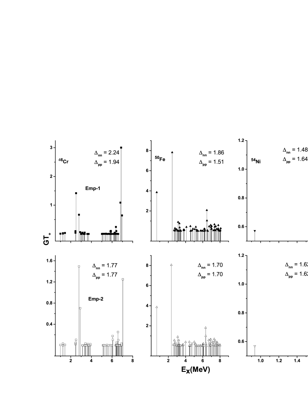
Figure 1: Calculated GT strength distributions for ⁴⁶Cr, ⁵⁰Fe and ⁵⁴Ni using pn-QRPA^(Emp-1) and pn-QRPA^(Emp-2) schemes.

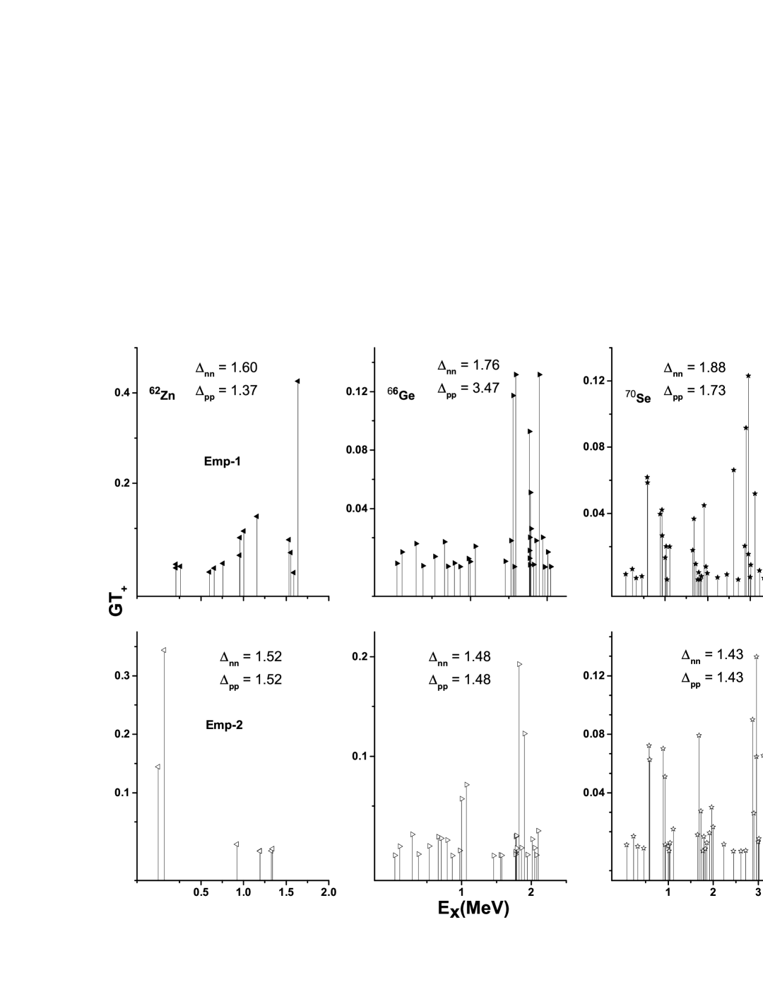
Figure 2: Calculated Gamow-Teller strength distributions for ⁶²Zn, ⁶⁶Ge and ⁷⁰Se using pn-QRPA^(Emp-1) and pn-QRPA^(Emp-2) schemes.

Fig. 1 depicts calculated GT strength distributions for ⁴⁶Cr, ⁵⁰Fe and ⁵⁴Ni using the two schemes. It is noted that calculated GT strength distribution changes appreciably for ⁴⁶Cr and remains more or less the same for ⁵⁰Fe and ⁵⁴Ni using the two different values of pairing gaps. Similarly Fig. 2 displays the corresponding result for ⁶²Zn, ⁶⁶Ge and ⁷⁰Se. The calculated strength distributions do change appreciably with change in values of $\Delta_{pp}(\Delta_{nn})$ (albeit less for the case of ⁷⁰Se).

Table 1 shows the value of total strength (in arbitrary units) and centroid (in MeV units) of the calculated GT strength distributions using different values of pairing gaps for all the nuclei considered in this paper. The last column mentions the cut-off energy in daughter up to which we show our calculation of total strengths and centroids (Columns V–VIII). It is noted from Table 1 that we have up to a factor four difference between the calculated total GT strengths using the two different pairing gaps. We would like to comment that in most instances the GT strength redistributes itself when the pairing gaps change. They shift to energies higher than the cut-off energy shown in the last column of Table 1. This explains the, at times, large differences in calculated total strengths and centroids. This also has an effect on calculated half-lives which we discuss in next table. It is clear from Table 1 that the pn-QRPA calculated GT strength distribution is a sensitive function of pairing strength parameter. The $S_{p}$ ($S_{n}$) dependent value of pairing strength ($Emp-1$) results in calculated half-lives in good comparison with measured data which we discuss next.

In Table 2 we display the performance of our model calculation. Shown are the pn-QRPA calculated half-lives along with previous half-life calculations and measured half-lives for selected even-even nuclei. The $Q$ values and experimental half-lives were taken from Ref. [17]. Column IV and Column V show our calculated half-lives using the $Emp-1$ and $Emp-2$ formulae for pairing strength. The last three columns display previous theoretical results. Column VI shows the calculated half-lives using the FRDM model [15] whereas the last two columns show the recent results of the EQRPA model [2]. Here we show both EQRPA results with and without the inclusion of proton-neutron pairing correlations. All entries are given in units of $s$. Comparison between measured data and pn-QRPA^(Emp-1) shows decent agreement. The calculated root mean square (RMS) deviation from measured data for $Emp-1$, $Emp-2$, FRDM, EQRPA(no-pn) and EQRPA(with-pn) model calculations are 272.6$s$, 5488.1$s$, 1734.6$s$, 3869.3$s$ and 3229.3$s$, respectively. The low RMS value achieved from $Emp-1$ model is a clear indication of the fact that the predicted half-life values are in decent agreement with the measured data. Noticeable differences in calculated pn-QRPA half-lives (using the $Emp-1$ and $Emp-2$ formulae) are seen for six cases. For the cases of ⁴⁸Fe, ⁵⁶Zn and ⁶⁰Ge the $Emp-2$ calculated half-lives are considerably bigger than those calculated using the $Emp-1$ formula. The reason may be traced back to Table 1 where it is noted that total calculated GT strength using the $Emp-1$ formula is appreciably bigger than the corresponding strength using the $Emp-2$ formula. Bigger total strength translates to bigger rates and correspondingly smaller half-lives. For the nuclei ^60,62Zn and ⁶⁸Se the $Emp-2$ calculated half-lives are appreciably smaller than those calculated using the $Emp-1$ formula. It is noted, from Table 1, that for all these three cases the $Emp-2$ formula places the centroid of the GT distribution at considerably lower daughter excitation energies than those using the $Emp-1$ formula. This in turn translates into bigger rates and corresponding smaller half-lives. In addition, for the case of ⁶⁰Zn and ⁶⁸Se, the $Emp-1$ formula calculated total GT strength is also much smaller than those calculated using the $Emp-2$ formula. As a sample case, we present the state-by-state half-life calculations of ⁶²Zn in Table 3 using the $Emp-1$ and $Emp-2$ formulae for pairing strength. Shown also are the pn-QRPA calculated GT strengths, branching ratios $I_{(\beta^{+}/EC)}$ and partial half-lives $t^{par}_{1/2}$ for the mentioned case. The branching ratio $I$ for each transition was calculated using the following formula

$$I=\frac{T_{1/2}}{t^{par}_{1/2}}\times 100(\%),$$ (29)

where $T_{1/2}$ is the total half-life and $t^{par}_{1/2}$ is the calculated partial half-life of the corresponding transition. It is noted from Table 3 that it is the big branching ratio of 67$\%$ at 0.068 MeV in daughter ⁶²Cu that leads to a considerable decrease in the total calculated half-life in the $Emp-2$ scheme.

It is evident that $\beta$-decay half-lives obtained as a result of our $Emp-1$ scheme are in excellent agreement with the measured half-lives. We achieve better agreement with measured data than the previous calculations of Ref. [2] (using the EQRPA model) and Ref. [15] (using the FRDM model).

As mentioned earlier tuning of GT force parameters ($\chi$ and $\kappa$) can lead to good prediction power of the pn-QRPA model. In earlier calculations [5, 6], instead of searching for a parameterization of GT force parameters, the authors directly applied the determined values of $\chi$ and $\kappa$ (using a procedure to match the measured half-lives). The predicted half-life values were nonetheless very encouraging. In previous pn-QRPA calculations [5, 6] it was argued that pairing gap values have very little affect on calculated $\beta$-decay half-lives. Since our finding is otherwise we decided to compare our calculated half-life values with previous pn-QRPA calculation [6]. Table 4 compares the current $Emp-1$ scheme calculation with the previously published half-life values from Ref. [6]. In Table 4, pn-QRPA(H) represents pn-QRPA calculated half-lives using mass formula of Ref. [28]. Similarly pn-QRPA(G) and pn-QRPA(M) represent pn-QRPA calculated half-lives using mass formula of Ref. [29] and [30], respectively. We show comparison for only those nuclei where results were published earlier [6]. It may be noted that the half-lives calculated using the $Emp-1$ scheme are in good agreement with experimental half-lives. It is further noted that the pn-QRPA(M) predicted results are better than the pn-QRPA(G) and pn-QRPA(H) predicted half-lives and in good agreement with measured data and $Emp-1$ scheme.

4 Conclusions and Summary

In this paper we calculated $\beta^{+}$/EC decay half-lives using the pn-QRPA model for neutron deficient $fp$-shell nuclei. The $\beta$-decay properties of chosen nuclei have a key role to play in the nucleosynthesis problem. It was concluded that the pn-QRPA model, in a multi-shell single-particle deformed space with schematic interaction and reasonable choice of interaction constants $\chi$ for particle-particle and $\kappa$ for particle-hole parameters, results in accurate prediction of $\beta$-decay half-lives. It was shown that pairing gaps alter the calculated GT strength distributions. It was further demonstrated that $Emp-1$ formula for calculation of pairing gaps resulted in better prediction of calculated half-life values than by using $Emp-2$ scheme. Our calculated $\beta^{+}$/EC decay half-lives were in excellent agreement with the measured one and showed marked improvement over the former calculations. Because of the available large model space (up to 7$\hbar\omega$ ) our model can calculate the half-lives for any arbitrary heavy nucleus. It is expected that the current investigation would lead to a better and reliable calculation of $\beta$-decay properties of unstable nuclei. In future we wish to explore the effect of the two schemes ($Emp-1$ and $Emp-2$) on predicted half-life values for the case of electron emission and double beta decay processes.

Table 1: Comparison between pn-QRPA calculated Gamow-Teller strength distributions using different values of pairing gaps: $\Delta_{nn}^{(Emp-1)}$ , $\Delta_{pp}^{(Emp-1)}$ and $\Delta_{nn,pp}^{(Emp-2)}$. Shown are the calculated pairing gaps (in $MeV$), total Gamow-Teller strength, centroid and cut-off energy (in $MeV$) using the pn-QRPA($Emp-1$) and pn-QRPA($Emp-2$) scheme for selected nuclei.

Nucleus	$\Delta_{nn}^{(Emp-1)}$	$\Delta_{pp}^{(Emp-1)}$	$\Delta_{nn,pp}^{(Emp-2)}$	$\sum GT^{Emp-1}$	$\sum GT^{Emp-2}$	${\bar{E}^{Emp-1}}$	${\bar{E}^{Emp-2}}$	Ecutoff
42Cr	1.78	1.97	1.85	11.6	4.58	7.40	5.69	13.8
44Cr	2.07	1.78	1.81	1.66	1.69	0.45	0.45	13.9
46Cr	2.24	1.94	1.77	1.63	1.72	0.43	0.43	8.0
46Fe	3.04	1.79	1.77	10.7	10.9	6.43	7.03	13.5
48Fe	1.79	1.67	1.73	2.42	0.78	1.51	4.59	13.5
50Fe	1.86	1.51	1.70	26.6	26.6	4.37	4.22	8.1
48Ni	1.87	0.66	1.73	40.3	14.0	8.18	9.93	15.6
50Ni	2.09	1.86	1.70	10.4	2.89	6.98	5.39	12.7
52Ni	2.02	1.69	1.66	7.97	5.23	3.92	2.92	11.0
54Ni	1.48	1.64	1.62	1.71	1.71	0.002	0.002	11.0
56Zn	1.71	1.35	1.60	14.4	3.56	9.94	7.03	12.3
58Zn	1.90	1.23	1.58	11.3	25.1	5.30	4.68	9.2
60Zn	1.71	1.64	1.55	1.83	2.78	2.83	2.17	4.5
62Zn	1.60	1.37	1.52	0.98	0.51	1.10	0.06	1.6
60Ge	1.97	1.41	1.55	14.4	4.00	9.30	8.19	12.2
62Ge	1.30	1.21	1.52	13.7	10.7	6.90	7.25	10.0
64Ge	1.90	1.88	1.50	0.58	0.50	1.55	1.58	4.5
66Ge	1.76	3.47	1.48	0.58	0.66	1.05	1.26	2.0
64Se	1.60	1.42	1.50	15.9	14.3	6.87	7.20	12.7
66Se	1.55	1.44	1.48	14.7	6.57	4.36	3.15	10.6
68Se	1.94	2.08	1.46	3.85	8.99	3.18	0.57	4.7
70Se	1.88	1.73	1.43	0.99	1.05	1.24	1.19	2.4

Table 2: Comparison between experimental [17], pn-QRPA^(Emp-1), pn-QRPA^(Emp-2), FRDM model [15] and EQRPA model (with and without $pn$ pairing) [2] calculated half-lives. Q_β values were taken from Ref. [17] and given in units of $MeV$. All half-lives are given in units of $s$.

Nucleus	$Q_{\beta}$	$T^{[EXP]}_{1/2}$	$T^{[pn-QRPA(Emp-1)]}_{1/2}$	$T^{[pn-QRPA(Emp-2)]}_{1/2}$	$T^{[FRDM]}_{1/2}$	$T^{[EQRPA(no-pn)]}_{1/2}$	$T^{[EQRPA(with-pn)]}_{1/2}$
42Cr	13.7	0.013	0.013	0.013	0.045	0.013	0.012
44Cr	10.5	0.042	0.038	0.037	0.118	0.056	0.038
46Cr	7.60	0.224	0.218	0.209	0.671	0.404	0.375
46Fe	13.5	0.013	0.012	0.012	0.018	0.014	0.011
48Fe	10.9	0.045	0.042	1.123	0.059	0.037	0.034
50Fe	8.14	0.152	0.135	0.119	0.542	0.301	0.301
48Ni	15.6	0.003	0.003	0.003	0.005	0.005	0.002
50Ni	12.9	0.018	0.018	0.018	0.017	0.018	0.016
52Ni	10.5	0.041	0.039	0.039	0.077	0.056	0.052
54Ni	8.79	0.114	0.102	0.102	0.646	0.329	0.299
56Zn	12.7	0.032	0.029	0.285	0.083	0.025	0.021
58Zn	9.37	0.086	0.048	0.043	0.597	0.192	0.162
60Zn	4.17	142.8	142.5	37.33	$>$100	268.3	60.29
62Zn	1.62	33094	32101	7399	$>$100	39372	31372
60Ge	12.2	0.030	0.025	0.245	0.082	0.494	0.424
62Ge	10.1	0.129	0.117	0.081	0.868	0.125	0.102
64Ge	4.52	63.70	48.62	50.16	80.88	752.2	665.6
66Ge	2.12	8136	7452	9557	$>$100	25125	23144
64Se	12.7	0.030	0.028	0.030	0.097	0.022	0.020
66Se	10.7	0.030	0.031	0.033	0.648	0.073	0.065
68Se	4.71	35.50	35.06	0.759	42.32	17.69	17.68
70Se	2.41	2466	2041	1865	$>$100	3388	3387

Table 3: The state-by-state half-life calculations for ⁶²Zn using the Emp - 1 and Emp - 2 formulae for pairing strength. $E_{x}$ are daughter excited state energies in units of $MeV$. Shown also are the corresponding GT strengths, branching ratios $I_{(\beta^{+}/EC)}$ and partial half-lives. All half-lives are given in units of $s$.

$E_{x}^{Emp-1}$	$GT^{Emp-1}$	$I_{\beta^{+}/EC}$ [Emp-1]	$t^{par}_{1/2}$[Emp-1]	$E_{x}^{Emp-2}$	$GT^{Emp-2}$	$I_{\beta^{+}/EC}$ [Emp-2]	$t^{par}_{1/2}$[Emp-2]
0.206	0.01297	8.1880	3.92E+05	0.000	0.14427	32.849	2.25E+04
0.208	0.02066	12.997	2.46E+05	0.068	0.34368	66.717	1.10E+04
0.259	0.01591	9.0970	3.52E+05	0.921	0.01203	0.4000	1.84E+06
0.601	0.00384	1.1870	2.70E+06	1.194	0.00076	0.0090	7.99E+07
0.654	0.01223	3.3930	9.46E+05	1.194	0.00009	0.0010	6.56E+08
0.758	0.02285	5.0370	6.37E+05	1.325	0.00047	0.0030	2.75E+08
0.953	0.04047	5.3110	6.04E+05	1.340	0.00407	0.0210	3.52E+07
0.957	0.07971	10.339	3.10E+05	-	-	-	-
1.003	0.09434	10.576	3.03E+05	-	-	-	-
1.158	0.12661	7.8700	4.07E+05	-	-	-	-
1.164	0.42584	25.823	1.24E+05	-	-	-	-
1.534	0.07499	0.1370	2.34E+07	-	-	-	-
1.554	0.04646	0.0460	7.02E+07	-	-	-	-
1.588	0.00259	0.0000	7.60E+09	-	-	-	-

Table 4: Comparison of present pn-QRPA^(Emp-1) and previous pn-QRPA calculation [6] with measured half-lives [17]. All half-lives are given in units of $s$.

Nucleus	$T^{[EXP]}_{1/2}$	$T^{[pn-QRPA(Emp-1)]}_{1/2}$	$T^{[pn-QRPA(H)]}_{1/2}$	$T^{[pn-QRPA(G)]}_{1/2}$	$T^{[pn-QRPA(M)]}_{1/2}$
42Cr	0.013	0.013	0.033	0.025	0.012
44Cr	0.042	0.038	0.083	0.068	0.041
46Fe	0.013	0.013	0.031	0.024	0.015
48Ni	0.003	0.003	0.011	0.008	0.006
50Ni	0.018	0.018	0.018	0.014	0.015
60Ge	0.030	0.025	0.034	0.031	0.032
62Ge	0.129	0.117	0.086	0.082	0.083
64Se	0.030	0.028	0.033	0.032	0.030
66Se	0.030	0.031	0.073	0.072	0.071

References

- [1] Fermi, E., 1934. An attempt of a theory of beta radiation. ZP 88, 161.
- [2] Tan, W., Ni, D., Ren, Z., 2017. Calculations of the -decay half-lives of neutron-deficient nuclei. CPC 41(5), 054103.
- [3] Sarriguren, P., Rodriguez, R, A., Guerra, E, M., 2005. Half-lives of rp-process waiting point nuclei. EPJA 24, 193.
- [4] Takahashi, K., Yamada, M., Kondoh, T., 1973. -decay half-lives calculated on the gross theory. ADNDT 12, 101.
- [5] Staudt, A., Bender, E., Muto, K., Klapdor, H, V., 1990. Second-generation microscopic predictions of beta-decay half-lives of neutron-rich nuclei. ADNDT 44, 79.
- [6] Hirsch, M., Staudt, A., Klapdor, H, V., 1993. Microscopic predictions of /EC decay half-lives. ADNDT 53(2), 166-193.
- [7] Nabi, J, U., Klapdor, H, V., 1999. Microscopic calculations of weak interaction rates of nuclei in stellar environment for A= 18 to 100. EPJA 5, 337.
- [8] Wang, Z, Y., Niu, Y, F., Niu, Z, M., Guo, J, Y., 2016. Nuclear -decay half-lives in the relativistic point-coupling model. JPG 43, 045108.
- [9] Ni, D., Ren, Z., 2014. -decay rates of r-process waiting-point nuclei in the extended quasiparticle random-phase approximation. JPG 41, 025107.
- [10] Niksic, T., Marketin, T., Vretenar, D., Paar, N., Ring, P., 2005. -decay rates of r-process nuclei in the relativistic quasiparticle random phase approximation. PRC 71, 014308.
- [11] Marketin, T., Vretenar, D., Ring, P., 2007. Calculation of -decay rates in a relativistic model with momentum-dependent self-energies. PRC 75, 024304.
- [12] Liang, H, Z., Van, Giai, N., Meng, J., 2008. Spin-isospin resonances: A self-consistent covariant description. PRL 101, 122502.
- [13] Niu, Z, M., Niu, Y, F., Liang, H, Z., Long, W, H., Niksic, T., Vretenar, D., Meng, D., 2013. -decay half-lives of neutron-rich nuclei and matter flow in the r-process. PLB 723, 172.
- [14] Pinedo, G, M., Langanke, K., 1999. Shell-model half-lives for N= 82 nuclei and their implications for the r process. PRL 83, 4502.
- [15] Moller, P., Nix, J, R., Kratz, K., 1997. Nuclear properties for astrophysical and radioactive-ion-beam applications. ADNDT 66, 131.
- [16] Pantis, G., Simkovic, F., Vergados, J, D., Faessler, A., 1996. Neutrinoless double beta decay within the quasiparticle random-phase approximation with proton-neutron pairing. PRC 53, 695.
- [17] Audi, G., Kondev, F, G., Wang, M., Huang, W, J., Naimi, S., 2017. The NUBASE2016 evaluation of nuclear properties. CPC 41, 030001.
- [18] Muto, K., Bender, E., Oda, T., Klapdor, H, V., 1992. Proton-neutron quasiparticle RPA with separable Gamow-Teller forces. ZPA 341, 407.
- [19] Nilsson, S, G., 1955. Binding states of individual nucleons in strongly deformed nuclei. MFMDVS 29, 16.
- [20] Majid, M., Nabi, J, U., Daraz, G., 2017. Allowed and unique first-forbidden stellar electron emission rates of neutron-rich copper isotopes. APSS 362, 1.
- [21] Homma, H., Bender, E., Hirsch, M., Muto, K., Klapdor, H, V., Oda, T., 1996. Systematic study of nuclear -decay. PRC 54, 2972.
- [22] Nabi, J, U., Cakmak, N., Stoica, S., Zafar, I., 2015. First-forbidden transitions and stellar -decay rates of Zn and Ge isotopes. PSC 90, 115301.
- [23] Nabi, J, U., Cakmak, N., Zafar, I., 2016. First-forbidden -decay rates, energy rates of -delayed neutrons and probability of -delayed neutron emissions for neutron-rich nickel isotopes. EPJA 52, 5.
- [24] Nabi, J, U., Cakmak, N., Majid, M., Salam, J., 2017. Unique first-forbidden -decay transitions in odd-odd and even-even heavy nuclei. NPA 957, 1.
- [25] Hardy, J, C., Towner, I, S., 2009. Superallowed 0+ 0+ nuclear -decays: A new survey with precision tests of the conserved vector current hypothesis and the standard model. PRC 79(5), 055502.
- [26] Gove, N, B., Martin, M, J., 1971. Log-f tables for -decay. ADNDT 10, 205.
- [27] Moeller, P., Sierk, A, J., Ichikawa, T., Sagawa, H., 2016. Nuclear ground-state masses and deformations: FRDM. ADNDT 109, 1-204.
- [28] Hilf, E, R., Groote, H, V., Takahashi, K., 1976. CERN Report 76-13, 142.
- [29] Groote, H, V., Hilf, E, R., Takahashi, K., 1976. ADNDT 17, 418.
- [30] Moller, P., Nix, J, R., 1981. ADNDT 26, 165.