Landau levels in a time-dependent magnetic field: the Madelung fluid perspective
Nicolas Perez1,2 and Eyal Heifetz1
1 Department of Geophysics, Porter school of the Environment and Earth Sciences, Tel Aviv University, 69978 Tel Aviv, Israel
2 The Steinhardt Museum of Natural History, Tel Aviv University, 12 Klausner Street, 6901127 Tel Aviv, Israel
Abstract
We propose to revisit a fundamental quantum problem, namely the evolution of an electron’s wave function under a time-dependent magnetic field, with the dual perspective of the Madelung fluid. First we present an analysis of the problem in a quantum mechanistic fashion, based on a perturbation theory of the Landau levels, and next address the same problem with the Madelung equations. We show that the latter formulation does not only provide an intuitive derivation of the solution, but it also allows us to understand the diabatic character of quantum evolution in terms of mechanical energy transfers. The sloshing oscillations of the wave function can be then interpreted as the consequence of deviations from the balance between the magnetic force and the gradient of the Bohm potential in the Landau levels. This study shows that the Madelung fluid approach reveals analogies between a priori unrelated concepts from quantum mechanics and geophysical fluid dynamics.
Copyright attribution to authors.
This work is a submission to SciPost Physics.
License information to appear upon publication.
Publication information to appear upon publication.
Received Date
Accepted Date
Published Date
1 Introduction
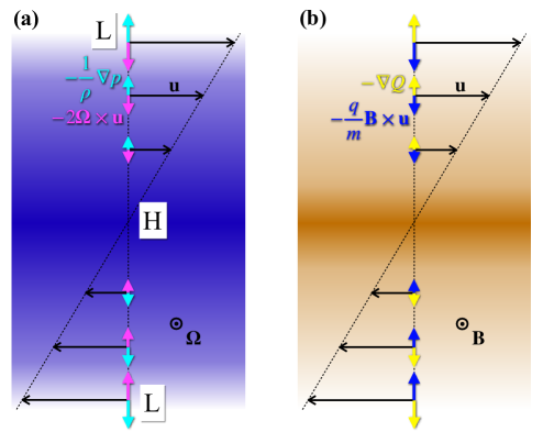
Less than a year after Schrödinger proposed his eponymous equation, Madelung showed an alternative formulation of it as a set of partial-differential equations describing a fluid [1], whose density and velocity fields are connected to the modulus and the phase gradient of the wave function. This conceptual fluid, known today as the Madelung fluid, was later used by Bohm [2] to revive and develop the pilot wave interpretation of quantum mechanics, formulated originally by de Broglie. The most relevant applications of Madelung hydrodynamics cover the study of Bose-Einstein condensates [3, 4], superfluidity and neutron stars [5, 6]. Besides, this formalism has regained attention in the recent years [7, 8], and it has been exploited for the purpose of bringing new insights on quantum problems based on their analogies with fluid dynamics [9, 10, 11, 12, 13]. In this perspective, Heifetz et al [12] demonstrated that the Madelung hydrodynamical equations associated to the Schrödinger equation of a two-dimensional charged particle in a transverse magnetic field are those of a compressible flow in a rotating frame, with zero absolute vorticity. They mapped the stationary solutions of the Madelung equations to the Landau levels of the charged quantum particle, thus providing a mechanistic interpretation of these eigenstates as steady plane Couette shear flows, in equilibrium under balanced forces acting perpendicularly to the flow: the gradient of the quantum (Bohm) potential, which acts from the center of the shear flow outward, and the Lorentz magnetic force, which acts inward. This is analogous to the geostrophic balance in high pressure systems, in the atmosphere and the ocean: the pressure gradient force acts outwards, whereas the Coriolis force acts inwards (Figure 1).
In this paper, we examine the non-stationary dynamics of the Madelung fluid when the flow is set out of balance. One way to do this is to consider that the initial wave function is an eigenstate of the Schrödinger equation – i.e. that the corresponding Madelung flow is stationary – and change the magnetic field with time, the question being that of the subsequent dynamics of the wave function and the corresponding Madelung flow. This particular problem has been addressed in different works with the perspective of emphasising specific dynamical properties of the Landau levels under time-varying parameters. It thus naturally relates to the quantum adiabatic theorem [14, 15], which has triggered a lot of interest owing to the great importance of geometric phases in driven condensed matter systems [15, 16]. For instance, the study of [17] exhibits geometric phases in Landau level dynamics with time-dependent electric fields under adiabatic conditions, while [18] focuses on interlevel transitions with a time-dependent transverse magnetic field under adiabatic or non-adiabatic conditions. To our knowledge, the only relatively recent work that proposed a hydrodynamical perspective to this problem – although not with the Madelung transformation – is [19]. It deals with a more general problem of one-dimensional -body system with inverse-square-potential pair interactions and a time-varying harmonic trap, but only addresses the dynamics of its coherent states. The analysis reveals a sloshing behavior of these coherent states, and proposes to associate it to persistent oscillations in one-dimensional superfluids.
We address the problem of Landau levels dynamics under a time-varying transverse magnetic field with a fluid perspective, through the Madelung formulation. However, for the sake of comparison and familiarity, we first present the problem in a quantum mechanics fashion, similar to [18], which allows us to obtain a perturbative expression of the wave function through the so-called squeezing operator. Next, we introduce the hydrodynamical formulation of the same problem, whose stationary solutions are plane Couette shear flows. We show that this formulation provides a mechanistic interpretation of the Landau level dynamics, which leads to an exact solution that is consistent with the sloshing behavior previously exhibited by [19], and is valid for all Landau levels. We show further that this dynamics is related to the phenomenon of geostrophic
adjustment in geophysical fluid dynamics, that we can in turn relate to quantum diabaticity with the problem of Landau level evolution under a time-dependent magnetic field. We then derive the energy constant of motion of the linearized dynamics of small perturbations (denoted in geophysical fluid dynamics as pseudo-energy) whose positive-definiteness reveals both stability of the perturbations and the possibility for hysteresis behavior.
The goal of this paper is to demonstrate how the Madelung fluid approach provides a straightforward classical-like interpretation, followed by a trackable physical intuition, which leads to exact mathematical solutions for the evolution of time-dependent Landau levels.
2 Quantum mechanics perspective
In this section, we first revisit the quantum problem of a two-dimensional charged particle in a transverse homogeneous magnetic field and a basis of eigenstates of the corresponding Schrödinger equation, the celebrated Landau levels. Then, building upon [18], we propose to address the non-stationary case – with a time-dependent magnetic field – by expanding the wave function in a time-dependent basis, which allows one to separate the adiabatic and diabatic contributions of the evolution. Finally, we discuss the conclusions of this analysis regarding the quantum adiabatic theorem [14, 15].
2.1 Definition of the quantum problem, Landau levels
We consider a two-dimensional particle of mass and charge subjected to an external electromagnetic field , which is described by the Schrödinger equation
| (1) |
For a homogeneous transverse magnetic field , following [12], we can choose the Landau gauge111The electromagnetic potentials, and , are defined up to a gauge, whose choice has no influence on the dynamics of the Madelung fluid since they do not affect the hydrodynamical fields, see the definitions (24) in section 3.:
| (2) |
Generally speaking, the choice (2) is valid regarding the Maxwell equations as long as the typical variation time of remains large compared to the time it takes electromagnetic waves to travel through the system (quasi-static approximation), which is assumed here222Otherwise and together do not obey the induction equation.. From now on let us use only dimensionless quantities, obtained by dividing time by a time scale and the spatial coordinates by a length , chosen such that . We also use the dimensionless magnetic field (which we will always assume positive from now on)333In the case of a constant magnetic field, if and , then is the inverse of the cyclotron frequency and is called the magnetic length., so that equation (1) becomes:
| (3) |
with the Laplacian operator . The problem is now entirely defined by the initial condition and the function . Equation (3) being invariant in the direction (hereafter, this coordinate will be referred to as zonal, adopting the geophysical fluid dynamics jargon in the equivalent context444In this paper we aim to relate between the quantum mechanics and the geophysical fluid dynamics perspectives when addressing this problem, thus we use familiar jargons from the two disciplines.), thus we can consider Fourier modes of wave number in this direction. The stationary solutions of equation (3), in the case of a constant magnetic field reads:
| (4) |
Equation (3) then becomes a second-order differential equation in the coordinate (hereafter, this coordinate will be referred to as meridional):
| (5) |
which is the well-known eigenvalue equation of a quantum harmonic oscillator. Since the meridional direction is unbounded555The two-dimensional space is assumed to be unbounded throughout the paper., the physically acceptable solutions of (5) are the Hermite-Gauss functions:
| (6) |
These are known as the Landau levels. Each eigenfrequency is infinitely degenerated, since they are independent of the value of 666Note that this is not true anymore with boundaries in the direction, as the meridional invariance is then lost.. This reflects the gauge symmetry, as the Fourier modes result from the arbitrary choice of the Landau gauge. This means that any linear combination of eigenfunctions (6) with the same index is also an eigenfunction with the same eigenfrequency . Since the physical system is completely invariant in the meridional direction, the value of , which simply shifts the center of the wave function, is unimportant, even in the case of a time-varying magnetic field . Therefore, we will take in the rest of the paper, and thus the problem reduces to the one-dimensional harmonic trap.
2.2 Perturbative expression of the wave function, squeezing and interlevel transitions
Let us now describe the evolution of the wave function , starting in a Landau level and letting to vary in time. The evolution equation is
| (7) |
with the initial condition
| (8) |
where the functions are defined in expression (6) ( is now omitted) and . If varies very slowly, one can intuitively predict that the wave function remains close to at time (see the comments regarding the adiabatic theorem in 2.3). To quantify that, we consider the projection of the wave function on the time-dependent orthonormal basis :
| (9) |
which is directly inspired by the analysis of [15, 18]. The normalization of the wave function implies that the sum of over all positive integers is equal to 1, and we also have by definition of the initial state. This decomposition (9) amounts to writing the evolution of the wave function in a frame that follows the variations of . In the rest of this section, it will be convenient to adopt a bra-ket notation for the functions of : we represent the function with the ket . This notation will be particularly convenient to use the Hermitian product defined by:
| (10) |
We will also denote the eigenfunctions and eigenvalues simply by and respectively, but always keeping in mind that they are time-dependent through . Injecting expression (9) into equation (7) and projecting on the basis function of a given level , one gets:
| (11) |
where we note the time-differentiation . The sum in the RHS of equation (11) contains only interlevel terms (). To see that, we recall that the functions are real-valued and normalized, therefore:
| (12) |
For the terms in the sum, we can show that777This is equation (8) in [15].:
| (13) |
where is the differential operator in the RHS of equation (7). Therefore, is equal to the operator . Using the formulation of with time-dependent ladder operators888These are such that , where † indicates the adjoint. We have and . They act on the eigenfunctions as and . and , we get:
| (14) |
which yields the following formulation of equation (11):
| (15) |
The recurrence relation (15) can be recast into a single equation, introducing the vector of the projection coefficients, :
| (16) |
where the ladder operators and are defined such that
| (17) |
Several comments can be made about expression (16):
-
•
First of all, it is a Schrödinger equation in a space that represents the time evolution of the basis of eigenstates. The first term in the RHS of (16) represents the adiabatic (or geostrophic-like, as we will explain in section 3) contribution, i.e. the dynamical part that consists in the Landau levels simply following the changes of the magnetic field . Without the second term, any eigenstate at remains an eigenstate (in the same level ) at time .
-
•
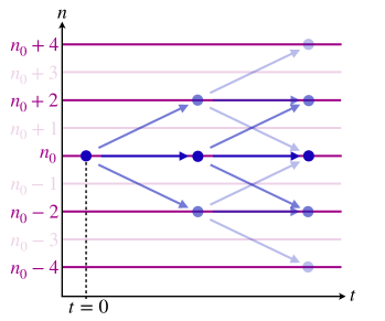
The second term in the RHS – which was alternatively obtained in [18] with a Klein-Gordon formulation of the problem – represents the diabatic part of the evolution, which quantifies the wave function departing from the expected Landau level . This term generates interlevel transitions between a level and the levels (Figure 2)999The levels do not interact with the level during the evolution as a result of parity symmetry being preserved by varying with time: an eigenstate of level has the same parity as in the direction, which is preserved during the evolution..
-
•
Finally, the fact that the term in is non-diagonal is symptomatic of the absence of geometric or Berry phase during the evolution process. This comes from (12), which is characteristic of the absence of phase in the eigenstates and the one-dimensional nature of the problem. If the problem is regarded in higher dimension or with more varying parameters (for instance an electric field or another component for the magnetic field), then a geometric phase may arise in the evolution, as in [17].
In order to focus on the effect of the second term in equation (16), we will adopt the interaction picture [20] and define the vector:
| (18) |
where we have noted . The transformation (18) separates the dominant dynamical phases of the wave functions – i.e. the terms that describe the respective adiabatic evolution of each coefficient – from the interlevel evolution, which underlies the diabatic evolution. Inserting (18) into (16) yields:
| (19) |
Therefore we can express the vector at time as:
| (20) |
The final expression in (20) is a time-ordered101010A time-ordered exponential differs from the natural exponential typically when the operators and do not commute for [20]. This is what happens here, so there is no exact expression of the evolution operator as far as we know. version of the so-called squeeze operator, which is a well-known evolution operator in the fields of quantum optics and quantum information. Although we do not have an exact expression for , it provides a natural perturbation formula for the diabatic effects when the integral of remains very small, i.e. if is varied very slowly, close to adiabaticity. Keeping only the first-order term in the expression in the second line of (20), we have:
| (21) |
Expression (21) merely expresses the rate at which interlevel transitions occur, i.e. at which the neighboring levels are populated as a result of diabaticity. Coming back to the initial wave function, we get:
| (22) |
This approximate solution only takes into account the nearest interlevel transition terms (). In spite of this approximation, the amplitude factor remains difficult to express in general. Nevertheless, let us look at the asymptotical limit, assuming that converges to a final value when . Since is bounded and when , the function converges to a constant value , which is small if varies slowly111111Indeed, assuming that is monotonic without losing generality, we have when , which is finite.. Therefore, all the coefficients of the wave function converge to a constant amplitude times the dynamical phase factor121212This result can be extrapolated to the full wave function. Expanding the evolution operator to all orders, one can show that it converges to a constant operator at infinite time. . Besides, the function is asymptotically equal to a constant plus the linear function , therefore we have:
| (23) |
as . To conclude, if the magnetic field converges to a final value , the modulus of the wave function eventually oscillates periodically with frequency around the adjusted Landau level’s modulus , and these oscillations do not fade. This result is still true with the full expansion of the evolution operator, since the phase difference between every interlevel term and the main coefficient is a multiple of . The final oscillating dynamics is thus the result of both symmetry being preserved and the Landau levels involved in the evolution being separated by frequency gaps that are all multiples of . However, it is not easy to compute the coefficient , nor to predict the amplitude of the final oscillations with this perturbative approach.
2.3 Remarks on the adiabatic theorem
The previous analysis must be addressed in light of the adiabatic theorem in quantum mechanics [14, 15]: generally speaking, if a Hamiltonian varies slowly (adiabatically) and its discrete eigenvalues remain sufficiently separated, then a quantum system initially prepared in the eigenstate remains in the same state (whose eigenvalue is a function of time) [15]. Such evolution of the wave function is adiabatic in the sense that the information on the state is preserved in time. A requirement for adiabaticity is that the typical time of variation of must remain large compared to , where is the energy gap that separates from the closest energy level of . Expression (22) illustrates the limitation of this theorem: the leading-order term of the wave function corresponds to the Landau level adjusted to the value , and the corrective interlevel terms at first order are proportional to , whose amplitude vanishes in the adiabatic limit, i.e. for infinitely slow variations of .
When the wave function is initially prepared in a Landau level before varying , we can intuitively understand why a strictly adiabatic behavior is not possible: as varies, the width of the effective harmonic trap changes and thus the wave function is squeezed, which induces a non-zero probability current in the meridional direction , i.e. a non-uniform phase of the wave function. Therefore, the intermediate state cannot correspond to any Landau level, since the latter do not have non-uniform phase factors. But what if the parameter executes a cycle, i.e. eventually goes back to the initial value ? This situation is the most meaningful regarding the questions of quantum diabaticity and loss of information of the wave function. Unfortunately, the mathematical approach adopted in this section does not allow to establish a conclusion. As we will see in section 3, the Madelung formulation provides a much clearer perspective regarding this matter, as it will allow us to express quantum diabaticity in terms of non-stationarity of a fluid flow, thus understand it in terms of out-of-balance forces and mechanical energy exchanges.
3 Fluid mechanics perspective
We will now introduce the Madelung equations relative to the present problem, the purpose being to demonstrate how the hydrodynamical perspective provides an exact solution to the time-dependent problem (7)-(8) that is straightforwardly interpretable in terms of body forces. After reminding that the Madelung equivalent of the Landau levels are shear flows in geostrophic-like balance, we derive an exact solution of the problem. This analysis establishes a direct analogy between quantum diabaticity and the process of adjustment in geophysical flows. Finally, we propose to analyze the result in terms of pseudo-energy of the perturbed flow.
3.1 Madelung hydrodynamics and Landau levels as geostrophic-like states
Madelung showed in 1927 that the Schrödinger equation can be mapped onto a set of dynamical equations that resemble those of a hypothetical perfect compressible fluid with a peculiar non-local enthalpy, the Bohm potential. The density and velocity fields in these equations are related to the modulus and the phase gradient of the wave function, solution of the initial Schrödinger equation. Real fluids consist in many particles and their continuous field equations imply the introduction of pressure, which reflects the microscopic interactions between the numerous particles. Conversely, the flow of the Madelung fluid reflects the underlying dynamics of a single quantum particle, which obeys hydrodynamical equations in which the non-local nature of the single particle itself is embedded.
Employing the polar expression of the wave function ( and are real-valued functions), the general equation (1) is mapped onto a set of nonlinear compressible Euler fluid equations. Indeed, defining:
| (24) |
respectively as the density, velocity field and the Bohm potential associated with the Madelung fluid, the real and imaginary parts of equation (1) yield:
| (25) |
| (26) |
Equation (25) is the equation of mass conservation and (26) is the Hamilton-Jacobi equation, which is equivalent to the time-dependent Bernoulli equation of a barotropic flow with enthalpy [9]. Taking the gradient of equation (26) and using the definitions (1) and (24) of the electric field and the velocity field , respectively, yields:
| (27) |
Furthermore, assuming that the phase of the wave function is regular131313In this paper we assume that has no point topological defect, so that the curl of its gradient is zero everywhere. In other situations it may not be so [7, 8], in that case the singularities of the wave function generate quanta of non-zero vorticity, i.e. quantized vortices [21]., the curl of is solely imposed by the magnetic field, as:
| (28) |
where is the cyclotron frequency vector. Besides, recalling the general relation:
| (29) |
we can finally rewrite equation (27) as an Euler momentum fluid-like equation:
| (30) |
Defining the material derivative of a ‘fluid parcel’, , the LHS of equation (30) corresponds to its acceleration while the RHS is the sum of the electromagnetic force (per unit of mass), and the Bohm potential gradient, which acts as an additional force. The Madelung fluid has the following properties:
-
•
The fluid is compressible as nothing imposes the divergence of to vanish. In fact, in the Landau gauge, the divergence of the vector potential is zero, so , i.e. the phase can be regarded as a source of compressibility [10]. Besides, total mass is conserved as a consequence of normalization of the wave function.
-
•
The quantum enthalpy or Bohm potential follows a barotropic but non-local thermodynamical law, i.e. it depends not only on the fluid’s density but also its derivatives [9]. While the relation between pressure and density in real fluids mirrors their thermodynamical properties, the quantum enthalpy translates wave-particle duality.
-
•
The vorticity of the flow (i.e. ) is imposed by the magnetic field, as expressed by equation (28). Under an electromagnetic field, the charged particle is subjected to the Lorentz force, whose magnetic part acts exactly like the Coriolis force for a fluid in a rotating frame141414On a side note, we find it edifying that Madelung hydrodynamics maps the effect of the magnetic field – which breaks time-reversal symmetry in quantum mechanics – onto the Coriolis effect, which also breaks time-reversal symmetry in classical fluid dynamics. We believe this has a pedagogical interest, as the fact that rotation breaks time-reversal symmetry might be more comprehensible to a common reader than the similar attribute of magnetic fields in quantum mechanics.. The cyclotron frequency is equivalent to the Coriolis parameter , which is equal to twice the angular frequency of the rotating frame. Viewed from a frame of rest, the total vorticity vector (known as absolute vorticity) is given by . For the Madelung fluid, (28) implies that the analogue absolute vorticity is strictly zero, denoted by [12] as zero absolute vorticity dynamics.
-
•
In addition to the magnetic Lorentz force, one can see from equation (30) that the Madelung fluid undergoes a body force – from definitions (1) and (2) – which is non-zero whenever the magnetic field varies (by inducing an electric field). As the zero absolute vorticity condition holds as well as when the magnetic field is time-dependent, the rotational part of the velocity varies accordingly and can be seen as a result of the work performed by the induced electric field.
In the rest of the paper, we will only use dimensionless quantities, as in section 2. The density and dimensionless velocity of the Madelung fluid read as
| (31) |
The velocity field is a superposition of a divergent () and a rotational () components. For a spatially independent vertical magnetic field , the rotational component is a plane Couette shear flow, whose vorticity is , satisfying by construction the zero absolute vorticity condition (28). It is also convenient to relate the mass flux151515While the velocity is ill-defined where vanishes, the mass flux is always correctly defined. In the Schrödinger picture, its integral yields the expected value of the particle’s velocity whereas, in the fluid picture, it yields the net mass transport across the plane. to the wave function:
| (32) |
where stands for the imaginary part of a complex number and its conjugate.
Eigenstate solutions of the Schrödinger equation are mapped onto the steady states (stationary solutions, denoted hereafter by overbars) of the continuity (25) and the momentum (30) equations (i.e. and ) [12]. For a constant magnetic field, the eigenstate solutions defined by equations (4)-(6) (with 161616Consistently with the argument at the end of subsection 2.1, the medium is invariant in the zonal direction, thus the position of the center of the stationary flow, given by , can be redefined as ., so that ), are translated to
| (33) |
The continuity equation becomes anelastic:
| (34) |
and the Hamilton-Jacobi equation becomes the time-independent Bernoulli equation, with equal to the Bernoulli potential:
| (35) |
where , as defined by expression (24). Equation (35) is equivalent to the quantum harmonic oscillator equation (5), with . As opposed to classical fluids, in the Madelung fluid the Bernoulli potential can only take discrete values. This results from the particular structure of the Bohm potential (24), for which only the specific Hermite-Gauss functions of (6) can set the RHS of (35) to a constant value for the specific shear flow . This steady state velocity is exactly equal to the zero absolute voriticty plane Couette flow component. As for all planar shear flows, its nonlinear advection term vanishes (), leaving the steady state solution in balance between the gradient of the Bohm potential and the magnetic force: . As pointed out by [12], this is equivalent to the geostrophic balance between the pressure gradient force and the Coriolis force in a rotating shallow water model (Figure 1), common to describe geophysical fluid systems [22]. For the Landau levels (6), the balance is in the meridional () direction, while the shear flow is in the zonal () direction:
| (36) |
as illustrated in Figure 1.
3.2 Diabaticity - deviating from geostrophy by varying : exact solution
Let us now address the time-dependent problem (7)-(8) with the hydrodynamical formulation. In the scope of this analogy, it corresponds to the following scenario: the initial Madelung flow is in geostrophic balance (Figure 1(b)), equation (36) (), i.e. such that (with and ), then imbalance is induced by changing the value of in time, which breaks the equilibrium between the Lorentz force and the gradient of the Bohm potential. For the one-dimensional () time-dependent Schrödinger equation (7), the density and velocity fields are independent of at any time, thus the corresponding two components of the Madelung momentum equation (30) and continuity equation (25) read as:
| (37) |
The zero absolute vorticity constraint yields immediately that the zonal momentum is equal to at all times. This implies an instantaneous171717Classical systems do not usually respond instantaneously to a change of external parameters. balance between the zonal component of the Lorentz force and the zonal momentum advection by the meridional component of the flow (so that ). Thus, the zonal component of the flow is changing only through the induced electric field . The second and third of equations (37) couple the density variations with the meridional flow . Using the material derivative , they can be equivalently written as:
| (38) |
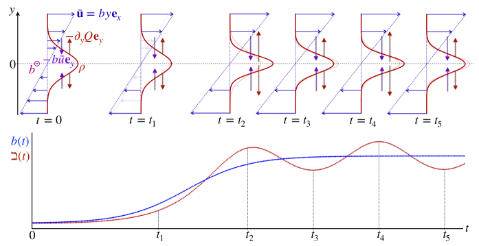
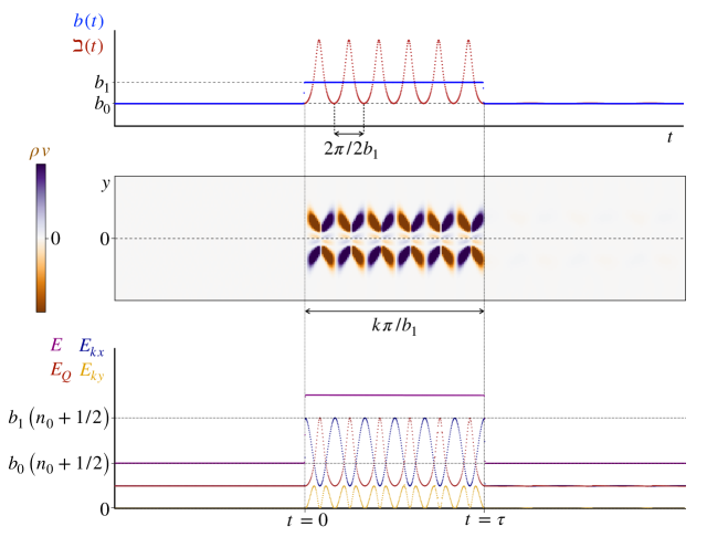
Initially, we have since the Couette flow is in geostrophic balance (). As begins to vary (say to increase), a non-zero meridional velocity arises and converges the density toward the center, which in turn alters , as demonstrated in Figure 3. Since the initial deviation from geostrophic balance is due to the increase in the magnetic Lorentz force, whose meridional component is proportional to , we can predict that the initial meridional acceleration of a fluid parcel at position is also proportional to . Moreover, since , we expect the generated flow to preserve the simple structure:
| (39) |
which is in agreement with the ansatz proposed by [19] for coherent states evolution. The continuous response of ‘fluid parcels’ thus exhibits the following properties:
| (40) |
Therefore, the density field is self-similar in time and reads as:
| (41) |
Remarkably, the properties (40) imply that the product is conserved with a fluid parcel’s motion () as varies181818In particular, if the initial state has lines of zero density, i.e. where (this is the case if ), these are preserved and move with the fluid parcels.. Plugging (39) in the first of equations (LABEL:eq:1D_dynamics), we obtain:
| (42) |
In other words, at any time , is an eigenfunction of the quantum harmonic oscillator with the time-dependent trapping frequency:
| (43) |
and eigenvalue . Since the initial conditions are and , we thus have:
| (44) |
We see that, while the velocity field is completely independent of the level number , is still the Hermite-Gauss function, so the density field has zeros in the meridional direction and vanishes away from the center over a typical distance , which characterizes the response of the Madelung fluid – initially in a state of stationary zonal flow – to the variation of . The self-similar character of the flow fields is consistent with the sloshing behavior191919In other words, the response of the Madelung fluid is a global, coherent meridional sloshing mode. already discussed in [19]. Expression (44), which is exact202020Keep in mind that this does not solve completely equation (7), as both and the phase of the wave function are yet to be found., provides an insightful alternative to the decomposition (9) of the wave function, as both formulations demonstrate an exact equivalence between the diabatic response of the quantum system and the ageostrophic dynamics of the Madelung fluid. Indeed, a flow that is constantly adjusted to the instantaneous value of would read , which also corresponds to the adiabatic evolution of the wave function. Nevertheless, even if the variation of the magnetic field is quasi-adiabatic, an initial plane-Couette stationary state cannot remain exactly stationary, for the following simple reason: as increases or decreases, the density field of the corresponding Landau level is compressed or decompressed in the meridional direction as the intensity of the zonal flow – and thus of the meridional Lorentz force – adjusts to the new value of (adiabatic expansion). This can only happen with a non-zero velocity field in , which means that the flow is not in geostrophic balance during the transition. Besides, in the expression (43) of , the term comes from the adjustment of the Lorentz force212121Note that the meridional Lorentz force is modified according to both the variation of and the corresponding instantaneous variation of ., whereas the term comes from the subsequent variations of (inertia). In other words, the difference between and – which characterizes the diabatic evolution of the quantum system – originates from the non-zero meridional velocity, which also embodies the ageostrophic dynamics of the Madelung fluid.
Comparing the solution with expression (41) allows us to identify:
| (45) |
therefore we obtain a second-order differential equation222222Equation (46) can be regarded as a remote variant of the Duffing equation, describing a nonlinear oscillator whose linear component has a time-dependent coefficient (parametric oscillator) and the forcing has the general form of . A major difference is that the term cannot be considered as a damping term. for :
| (46) |
Since and for a regular function , the driving term is the one that produces non-zero meridional velocity. Let us note that the solution of equation (46) – and thus the function as well – is completely determined by and is independent of the level index . In the regime of constant , say after varying to a new value , equation (46) becomes a nonlinear equation of free oscillations:
| (47) |
The linear part in equation (47) characterizes an oscillator of frequency , which is in agreement with the conclusions of section 2. The second term, which indicates the frequency of the persistent oscillations, arises from the Lorentz force – proportional to – and the properties of . Equation (46) for the general transiting regime cannot be solved analytically, however there is an exact solution of equation (47) for the permanent regime’s dynamics, and one can check (see appendix A) that it is given by232323This solution is consistent with expression (13) found in [19] for the coherent sloshing mode. As discussed in the introduction, the one-dimensional quantum problem (7) was analyzed by [19] in the context of a more general -body system with additional pair interactions and a solution was proposed for the coherent states. While the solution of [19] is derived after assuming an ansatz for the wave function, here the solution results directly from the Madelung formulation.:
| (48) |
where the constants are given by the value of and at some time to solve the Cauchy problem. In other words, expressions (48) is the exact solution in the permanent regime, and depend on the past evolution of . The smallness of the coefficient – which is the Madelung analog of the Rossby number [22, 12] – quantifies the adiabatic character of the quantum system. For instance, if is a step function that is equal to for and for 242424Let us note that this situation is the equivalent of having a constant value at all time and start with an eigenfunction with some , which is a non-stationary state., then the velocity field for is given by expressions (48) with and 252525Note that is indeed a small parameter for a small variation of , and its sign is in agreement with the expected sign of the meridional velocity field right after : for instance, if , is negative for and positive for , which is compatible with the compression of the density toward the center as the Lorentz force increases., which are compatible with and . These are exact expressions for . The wave function262626The phase of the wave function is determined through the definition and the Bernoulli equation . in the permanent regime (), under the condition that the wave function is initially a stationary (Landau) state for the initial value of the magnetic field , reads:
| (49) |
Expressions (48) reveal that the Madelung flow adopts a periodic behavior in the permanent regime, and that the frequency of the oscillations272727Note that expanding the denominator in the expression of provides an explicit decomposition in a Fourier series. is given by , as alternatively concluded in section 2. These periodic global oscillations of the Madelung fluid constitute a sloshing mode, which is the result of the restoring mechanisms of the Madelung fluid, owing to the Lorentz force and the gradient of Bohm potential (Figure 3). The slower is the variation of , the smaller is the amplitude of these oscillations, however expressions (48) and (49) are exact no matter the rate of change of . Eventually, the amplitude of the oscillations of is entirely determined by the memory of the transition through equation (46). This solution in the permanent regime naturally emerges as a consequence of the hydrodynamical interpretation of the adjustment problem, characterizing quantum diabaticity and providing an interpretation for the frequency of the reminiscent oscillations as a manifestation of interlevel transitions.
3.3 Sloshing energetics and pseudo-energy
In the previous analysis, we showed that any change of to a new constant value leads to a new Madelung flow that is the superposition of the adjusted stationary flow and a persistent oscillation in the meridional direction. In terms of energetics, during the adjustment process, there are two sources of available energy: the energy injected in the flow through the variation of 282828More specifically, energy is injected to the flow via the work of the induced field that appears in the zonal momentum equation (37). with time, and the initial background flow energy, which is the sum of Bohm’s potential energy and zonal kinetic energy. To understand the mechanisms of energy partitioning between the oscillation and the adjusted mean flow, let us identify and compute these different contributions. Generally speaking, the energy of the Madelung flow can be expressed as292929Let us remind that we consider flows that do not depend on the zonal coordinate .:
| (50) |
where the operator is the one expressed in equation (7). Therefore, the total amount of energy absorbed by the system (provided by the induced electric field, i.e. the external variation of ) per unit of time is equal to:
| (51) |
We can make a few comments about expression (51). In the Madelung fluid perspective, it corresponds to the work of the induced electric field on all the fluid parcels of mass and zonal velocity , per unit of time. If were not varying in time, then all the work would be converted into zonal kinetic energy, and if were to execute a cycle – i.e. come to its initial value – then the total work would be zero, as the integral of (51) would vanish. However, we can see that the work injected not only depends on the field strength ( and ), but also on the mass distribution during the time work is performed – i.e. the function – which is characteristic of a parametric oscillator. Owing to this property, we can already expect situations of energetic hysteresis, in which the net injection of work is non-zero even if eventually comes back to its initial value. Starting in the Landau state for the initial value , we can show (see appendix B) that the rate of energy injection is:
| (52) |
At initial time , the total energy of the flow is equal to and it is equally partitioned between zonal kinetic energy and Bohm’s potential energy [12]. This is not true anymore for . Indeed, because of the properties of the function , we have303030Expressions (53) reveal that equipartition between zonal kinetic and potential energy is possible only if , which would correspond to the exact adiabaticity of the quantum system. (see appendix B):
| (53) |
One can check that the total energy is indeed equal to at (as initially ), and that:
| (54) |
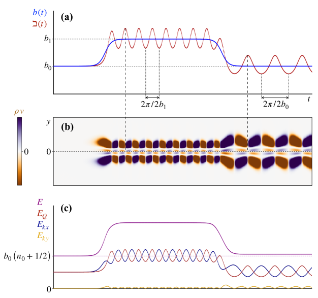
for , i.e. that the energy of the flow is systematically higher than the expectation energy of the adjusted mean flow. In other words, there is always a positive amount of energy which corresponds to the generation of persistent oscillations (Figure 4). Energy is injected to or extracted from the flow by the external action of the induced zonal field , and expression (52) shows that the sign of determines whether the energy is injected or extracted. If executes a cycle such that its initial and final values are equal, the additional energy in (54) does not vanish in general, which is symptomatic of a diabatic evolution of the quantum wave function. Rather than a perfect adjustment of the flow to a new geostrophic-like state, we thus observe an energetic hysteresis owing to the systematic generation of these oscillations, which may not be reversed simply by returning to its initial value. This hysteresis phenomenon thus characterizes the diabaticity of the quantum system in terms of global waves persisting in the Madelung fluid.
The final state is a geostrophic one if and only if expression (54) vanishes, i.e. (no transverse motion) and , which can be achieved only in marginal cases depending on how the variations of are synchronized with the oscillations of the flow. Let us consider a simple example in which varies stepwise313131In other words varies only over a time scale that is much smaller than ., going from to at time and back to at time . For the flow to come back to its initial state, i.e. for the oscillations initiated at to be suppressed, the total energy balance must be zero, i.e. the integral of expression (51). Since energy is injected or removed only at times and , this integral can be expressed as:
| (55) |
which is zero if and only if is chosen such that (Figure 5). This is consistent with the general form (48) of the solution on intervals of constant : since and are continuous, must be returned to the initial value when , which coincides with the cancellation of meridional velocity323232During the time interval , the function oscillates between the values and with frequency , as can be noticed from expression (48), so is an extreme value of . and times with integer . This behavior can be related to that of classical parametric oscillators, for which some property of the system can grow or decay depending on how the variations of a parameter are synchronized with the oscillations of the system itself.
Alternatively, we can compute the pseudo-energy of the oscillations under the linear approximation. We assume that the permanent regime is established ( and ) and the Madelung flow is the superposition of the corresponding geostrophic-like state and some perturbation333333As stressed in [13], any linear combination of wave functions that solve the Schrödinger equation is still a solution of it, however the superposition of their respective Madelung flows is not a solution of the hydrodynamical equations, in general., i.e. and with . We can thus write the total energy as:
| (56) |
By definition, is equal to , which is the energy of the unperturbed geostrophic flow. Using expression (24) and the Taylor expansion , Bohm’s potential can be written as:
| (57) |
up to order square in the perturbation fields, for the purpose of computing the pseudo-energy. Bearing in mind that conservation of mass implies 343434Indeed, ., and keeping terms only up to quadratic order in the perturbations, we can show the following expression of the pseudo-energy:
| (58) |
Thus, up to quadratic order, the pseudo-energy is a constant of motion (in the permanent regime), which is positive definite in the perturbations, consistently with (54)353535However, expression (58) is valid for general small perturbations of the permanent stationary flow, not only the situation in which varies to a different permanent regime, which yields expression (54).. Hence, the Madelung flow is stable to perturbations, a fact that could be anticipated from the start owing to the Hermiticity of the quantum system. Expression (58) is characteristic of the Madelung fluid, as the potential contribution (i.e. the second term in RHS) depends on the derivative of the density perturbation. This expression is the counterpart of expression (22) derived in [11]. It is the energy of small perturbations of a stationary plane-Couette flow, in particular of the persistent sloshing oscillation accompanying the adjustment process, whose energy is alternatively exactly given by (54). The background density has zeros (for ) – contrary to the non-rotating scenario depicted in [13] –, which compromises the well-definiteness of the potential term as expressed in (58), and of the expansion (57) itself. This challenges local linear approximations and is symptomatic of the sloshing mode being a global motion of a self-similar oscillating solution.
3.4 Geostrophic adjustment in the Madelung fluid and in shallow-water systems: discussion
In light of the analogy between the Madelung fluid and two-dimensional rotating flows, it is insightful to compare the ageostrophic/diabatic dynamics explored in 3.2 to the evolution of shallow-water flows. In such a system, if a perturbation occurs such that geostrophic balance is not established, the flow then naturally relaxes toward a new geostrophic state by emitting away transient inertio-gravity (Poincaré) waves, which transport and redistribute energy and momentum while leaving potential vorticity unchanged. The theory behind this phenomenon, called geostrophic adjustment, was originally formulated by Rossby [23], and developed further in the following decades [24, 25, 26, 27]. The first experimental confirmations of the theory, by means of observations in oceanic currents, came only in the late seventies [28, 29]. Recent observations of the hurricane Milton from space provides a graphical demonstration of geostrophic adjustment: as the cyclone’s pressure gradient varied owing to the encounter with land or other meteorological phenomena, its rotation rate adjusted to the new geostrophic balance while emitting gravity waves away from the storm’s center [30]. In two-dimensional flows, the phenomenon of geostrophic adjustment essentially relies on the conservation of potential vorticity and the fact that transient inertio-gravity waves do not transport it, whereas they can transport energy and momentum in order to adjust pressure and mass distribution to converge to a new geostrophically-balanced flow.
In contrast with geofluids, the vorticity of the Madelung fluid is imposed by the cyclotron vector everywhere, which is a very constraining property that prevents the existence of similar propagation phenomena such as Poincaré and Rossby waves altogether, essential to the geostrophic adjustment of geophysical flows. Moreover, the persistent oscillations of frequency previously exhibited are in striking contrast with the adjustment of geostrophic flows where the final state is geostrophically balanced. In the geophysical context, there are possible obstructions to geostrophic adjustment, such as instabilities or the presence of boundaries where the transient inertio-gravity waves reflect and thus are unable to be emitted away from the flow. However, the Madelung fluid discussed throughout this paper is unbounded and a priori stable to any kind of perturbation, owing to the Hermiticity of the quantum system, yet it does not adjust to a new balanced state when reaches a new constant value. As discussed in [13], the Madelung fluid locally supports de Broglie waves, but those cannot propagate away from a stationary flow that corresponds to a Landau level, since the Madelung fluid’s density vanishes as increases. In other words, far from the density center, there is no support for these waves to be emitted away, in contrast with transient gravity waves in open shallow-water systems.
4 Conclusion and outlooks
The Madelung representation of the electron’s wave function describes a perfect compressible fluid whose dynamics obeys specific mechanisms that characterize the quantum nature of the wave function. Under a magnetic field, the Madelung fluid is subjected to a Lorentz force but its absolute vorticity remains strictly zero. On the other hand, the fluid is subjected to its Bohm potential, which is a function of the density that reflects the non-local nature of this fluid. These peculiar properties result in exotic hydrodynamical behavior of the Madelung fluid, which can still be related to that of classical fluids, as far as particular situations are concerned. For instance, if the magnetic field varies slowly, the quasi-adiabatic evolution of the wave function is the exact analog of the quasi-geostrophic adjustment of shallow-water flows. However, while the adjustment of classical shallow-water flows is accompanied by the emission of transient inertio-gravity waves – that result in the convergence of the flow to a new geostrophic state with unchanged potential vorticity –, the adjustment of the Madelung fluid is accompanied by persistent sloshing oscillations that vanish only in marginal cases, even if the magnetic field is eventually set back to its original value. The quasi-irreversible generation of this oscillating motion – which is a single, global non-linear mode with a self-similar structure, that oscillates exactly at twice the cyclotron frequency – is characteristic of the response of superfluids – which are dissipationless – to perturbations. Such response strongly differs from classical fluids, for which the theory of geostrophic adjustment predicts that the persistence of inertio-gravity oscillations is possible only with instability or wave reflection at boundaries, none of which is needed for the sloshing of the Madelung fluid. Besides, the constraint of zero absolute vorticity implies a profound difference in the restoring mechanism of the rotating Madelung fluid, as it constitutes an obstruction to Le Chatelier’s principle. In the situation depicted throughout the paper, the response of the Madelung fluid is one-dimensional as the zonal velocity is enslaved to the instantaneaous value of (Figure 3). On the contrary, for a similar shallow-water flow, the generation of non-zero meridional velocity would produce a zonal Coriolis force and thus drive additional zonal velocity in the opposite direction as the original zonal flow, i.e. a counter-effect, which is essential to geostrophic adjustment.
The hydrodynamical perspective adopted in this paper allowed us to provide an exact solution to the initial quantum problem, whereas the traditional perturbation theory presented in 2.2 only led to an approximate one. Our derivation relied on the mechanistic interpretation of the Landau levels as stationary plane-Couette flows in geostrophic-like balance, which allowed us to establish an analogy between quasi-geostrophic dynamics and quasi-adiabatic quantum evolution. We reported a natural connection between quantum diabaticity and mechanical energy exchanges in the Madelung fluid, and successfully connected it to the pseudo-energy, which quantifies the irreversibility of the quantum system in terms of ageostrophic dynamics of the fluid. We expect that this analogy goes beyond the context of this paper and can be insightful in other situations. To name a few, possible follow-up studies could for instance i/ include mean-field quantum interactions (with the Gross-Pitaevskii equation363636Curiously, while the linear Schrödinger equation yields non-linear Madelung equations, adding the non-linear term of the Gross-Pitaevskii equations results in a barotropic enthalpy contribution that is simply proportional to the density .) and their competition with the Bohm potential (local interactions against non-local quantum effects), ii/ add boundaries in the meridional direction, which is expected to drastically modify the Landau level dynamics for Couette flows centered near those boundaries, and iii/ include perturbations in the zonal direction (thus two-dimensional) in order to explore de Broglie wave dynamics (which would be in the continuation of [13]) or Berry phase effects.
Funding information
NP is funded by a scholarship from Tel Aviv University.
Competing/conflicting interests
The authors declare no conflict of interest.
Appendix A Solution of equation (47)
We derive here the unique solution of the non-linear differential equation (47) for the oscillations in the permanent regime (constant ). In order to do that, we define
| (A.1) |
By successive time differentiation of (A.1), we obtain
| (A.2) |
which, plugged into equation (47), yields
| (A.3) |
The general solution of (A.3) is (note that the solution is valid regarding the definition (A.1) only if ), therefore, defining , we have
| (A.4) |
which corresponds to expression (48). Furthermore, is obtained using the definition :
| (A.5) |
Noticing from (45) that , we can finally identify .
Appendix B Expression of energy integrals
In this appendix we provide the derivation of expressions (52) and (53), which are based on the mathematical properties of Hermite polynomials. We use the bra-ket notation and the ladder operators of 2.2, but define them for the trapping frequency instead of (this way the wave function derived in 3.2 is proportional to at any time, up to a phase factor that depends on and ). Thus, for the sloshing mode whose wave function is given by (49), we can write:
| (B.1) |
The terms coming from and in (B.1) vanish by definition of the action of the ladder operators. Moreover, since and the ladder operators obey the commutation rule , we finally have:
| (B.2) |
which proves expression (52). Similarly, the first two expressions of (53), i.e. the zonal and meridional kinetic energy of the flow and , follow straightforwardly from relation (B.2). As for the potential energy, using (42) and (44), we obtain:
| (B.3) |
References
- [1] E. Madelung, Quantum theory in hydrodynamical form, Z. Phys. 40, 322 (1927), 10.1007/BF01400372.
- [2] D. Bohm, A suggested interpretation of the quantum theory in terms of" hidden" variables. i, Phys. Rev. 85, 166 (1952), 10.1103/PhysRev.85.166.
- [3] P. A. Andreev and L. S. Kuz’menkov, Dispersion properties of transverse waves in electrically polarized becs, J. Phys. B: At. Mol. Opt. Phys. 47, 225301 (2014), 10.1088/0953-4075/47/22/225301.
- [4] P. A. Andreev, Quantum hydrodynamic theory of quantum fluctuations in dipolar bose–einstein condensate, Chaos 31, 023120 (2021), 10.1063/5.0036511.
- [5] J. A. Sauls, Superfluidity in the interiors of neutron stars, In Timing neutron stars, p. 457. Springer, 10.1007/978-94-009-2273-0_43 (1989).
- [6] L. V. Drummond and A. Melatos, Stability of interlinked neutron vortex and proton flux tube arrays in a neutron star: equilibrium configurations, Mon. Not. R. Astron. Soc. 472(4), 4851 (2017), 10.1093/mnras/stx2301.
- [7] M. Berry, Time-independent, paraxial and time-dependent madelung trajectories near zeros, J. Phys. A: Math. Theor. 57(2), 025201 (2023), 10.1088/1751-8121/ad10f2.
- [8] M. V. Berry, Kinetically anisotropic hamiltonians: plane waves, madelung streamlines and superpositions, Eur. J. Phys. 45, 045401 (2024), 10.1088/1361-6404/ad4f34.
- [9] E. Heifetz and E. Cohen, Toward a thermo-hydrodynamic like description of schrödinger equation via the madelung formulation and fisher information, Found. Phys. 45, 1514 (2015), 10.1007/s10701-015-9926-1.
- [10] E. Heifetz, R. Tsekov, E. Cohen and Z. Nussinov, On entropy production in the madelung fluid and the role of bohm’s potential in classical diffusion, Found. Phys. 46, 815 (2016), 10.1007/s10701-016-0003-1.
- [11] E. Heifetz and I. Plochotnikov, Madelung transformation of the quantum bouncer problem, Europhys. Lett. 130(1), 10002 (2020), 10.1209/0295-5075/130/10002.
- [12] E. Heifetz, L. R. Maas and J. Mak, Zero absolute vorticity plane couette flow as an hydrodynamic representation of quantum energy states under perpendicular magnetic field, Phys. Fluids 33, 127120 (2021), 10.1063/5.0075911.
- [13] E. Heifetz, A. Guha and L. Maas, de broglie normal modes in the madelung fluid, Found. Phys. 53, 35 (2023), 10.1007/s10701-023-00676-z.
- [14] M. Born and V. Fock, Beweis des adiabatensatzes, Z. Phys. 51, 165 (1928), 10.1007/BF01343193.
- [15] M. V. Berry, Quantal phase factors accompanying adiabatic changes, Proc. R. Soc. Lond. A 392(1802), 45 (1984), 10.1098/rspa.1984.0023.
- [16] D. Xiao, M.-C. Chang and Q. Niu, Berry phase effects on electronic properties, Rev. Mod. Phys. 82(3), 1959 (2010), 10.1103/RevModPhys.82.1959.
- [17] J. Chee, Landau problem with a general time-dependent electric field, Ann. Phys. 324(1), 97 (2009), 10.1016/j.aop.2008.08.005.
- [18] S. P. Kim, Landau levels of scalar qed in time-dependent magnetic fields, Ann. Phys. 344, 1 (2014), 10.1016/j.aop.2014.02.009.
- [19] B. Sutherland, Exact coherent states of a one-dimensional quantum fluid in a time-dependent trapping potential, Phys. Rev. Lett. 80(17), 3678 (1998), 10.1103/PhysRevLett.80.3678.
- [20] H. Bruus and K. Flensberg, Many-body quantum theory in condensed matter physics: an introduction, Oxford University Press, 10.1093/oso/9780198566335.001.0001 (2004).
- [21] G. E. Volovik, The universe in a helium droplet, Oxford University Press, 10.1093/acprof:oso/9780199564842.001.0001 (2009).
- [22] G. K. Vallis, Atmospheric and oceanic fluid dynamics, Cambridge University Press, 10.1017/9781107588417 (2017).
- [23] C. G. Rossby, On the mutual adjustment of pressure and velocity distributions in certain simple current systems, ii, J. Mar. Res. 1(3), 239 (1938), 10.1357/002224038806440520.
- [24] A. Cahn Jr, An investigation of the free oscillations of a simple current system, J. Atmos. Sci. 2(2), 113 (1945), 10.1175/1520-0469(1945)002<0113:AIOTFO>2.0.CO;2.
- [25] W. Blumen, Geostrophic adjustment, Rev. Geophys. 10(2), 485 (1972), 10.1029/RG010i002p00485.
- [26] J. Pedlosky, Geophysical fluid dynamics, Springer New York, 10.1007/978-1-4612-4650-3 (1987).
- [27] V. Zeitlin, Geophysical fluid dynamics: understanding (almost) everything with rotating shallow water models, Oxford University Press, 10.1093/oso/9780198804338.001.0001 (2018).
- [28] C. L. Tang, Inertial waves in the ‘gulf of st lawrence: A study of geostrophic adjustment, Atmos. Ocean 17(2), 135 (1979), 10.1080/07055900.1979.9649056.
- [29] C. Millot and M. Crépon, Inertial oscillations on the continental shelf of the gulf of lions—observations and theory, J. Phys. Oceanogr. 11, 639 (1981), 10.1175/1520-0485(1981)011<0639:IOOTCS>2.0.CO;2.
- [30] S. News, Watch: Hurricane milton seen from space as the storm crosses the gulf of mexico, https://news.sky.com/video/watch-hurricane-milton-seen-from-space-as-the-storm-crosses-the-gulf-of-mexico-13230548 (2024).