Anisotropic fluctuations of momentum and angular momentum of heavy quarks in the pre-equilibrium stage of pA collisions at the LHC

Abstract

We simulate the real-time evolution of the $SU(3)$-glasma generated in the early stages of high-energy proton–nucleus collisions, employing classical lattice gauge theory techniques. Our setup incorporates a realistic modeling of the proton’s internal structure and includes longitudinal fluctuations in the initial state, enabling the study of genuinely non-boost-invariant collision dynamics. Focusing on the momentum and angular momentum anisotropies of heavy quarks in the infinite mass limit, we find that the system retains significant anisotropy well beyond the characteristic timescale $\tau=1/Q_{s}$. This persistence of anisotropy is further confirmed in the more realistic, non-boost-invariant scenario, across a range of fluctuation amplitudes. These findings pave the way for future investigations involving dynamical heavy quarks and more quantitative initializations of the glasma.

I Introduction

The analysis of a relativistic heavy-ion collision, as performed at the Relativistic Heavy Ion Collider (RHIC) at Brookhaven National Laboratory and at the Large Hadron Collider (LHC) at CERN, provides a unique opportunity to investigate the behavior of QCD matter at extreme temperatures and densities. The study of such events requires different kinds of descriptions of the spacetime evolution of the system, since the matter produced in the collision experiences different stages in its evolution. For instance, over the past few decades many experimental results have indicated the emergence of a new state of matter, referred to as the Quark-Gluon Plasma (QGP), which forms after $\sim 1$ fm after the collision and in which quarks and gluons behave as a hydrodynamic fluid [1, 2, 3].

If we instead consider the early stages of the collision ($\leq 1$ fm), the Classical Yang-Mills (CYM) theory offers a good description of this phase. It can describe well the nonequilibrium evolution of the highly occupied gluonic system, called the glasma, that appears immediately after the collision. In particular, the glasma simulation with the CYM field plays an important role in understanding the nonequilibrium stage between the moment of the collision and the onset of the hydrodynamic evolution of the QGP. In fact the glasma simulation, in the analysis of experimental data, is widely used to establish the initial conditions for the subsequent hydrodynamic evolution [4, 5]. The theoretical background for why the CYM theory offers a good picture of the initial gluonic matter is based on the Color Glass Condensate (CGC) framework, which stands as a valid description of the high-energy nucleus [6, 7, 8], see [9, 10, 11, 12] for reviews. In such a high-energy nucleus the dominant degrees of freedom are soft gluons emitted from hard partons. In particular, the McLerran-Venugopalan (MV) model in the CGC effective theory describes the soft gluons as the CYM fields and the hard partons as their color sources. Consequently, the glasma generated in the collision of such high-energy nuclei can be described well by the CYM field. The greatest simplicity of the CGC formalism is the fact that the complexity of a non-linear many-body problem at high energy is reduced into a one-scale problem, with a hard saturation scale $Q_{s}$ as the only dimensionful relevant scale at which gluon recombination effects start to become as important as the gluon radiation ones. The CYM equations can be studied both analytically (e.g. by employing a small time expansion [13, 14]) or numerically [15, 16].

However, such a success of the glasma simulations has been largely limited by the boost invariance assumption, which shows good agreement with experimental data only around the midrapidity region. Recently, much attention has been paid to the 3 + 1-dimensional (3 + 1D) glasma simulations, which aim to go beyond the boost invariance assumption, as necessary to understand observables across a broader region of rapidity [17, 18]. In fact, on top of the glasma it is possible to add quantum fluctuations [19, 20, 21, 22, 23, 24, 25, 26, 27, 28, 29, 30, 31, 32], which are known to trigger plasma instabilities [33] and are helpful to produce entropy during the early stages of high energy nuclear collisions [23, 34, 35, 36]. Quantum fluctuations appear when one considers the finite coupling corrections to the glasma solution (which is obtained in the small coupling limit): the spectrum of these fluctuations has been computed within a perturbative calculation in [24] and it has been shown that they affect both the gauge potential and the color electric field.

The experimental framework we mentioned refers to Pb-Pb (LHC) or Au-Au (RHIC) collisions. Moving on to measurements in smaller collision systems such as pp and pA [37, 38] (in particular those of anisotropies in multi-particle correlation functions), these have shown very similar features as those found in heavy ion collisions. While calculations within the hydrodynamic framework have been quite successful in describing observables in these small collision systems, alternative explanations relying entirely on intrinsic momentum correlations of the produced particles can also reproduce many features of the experimental data [37, 38]. It is likely that both initial intrinsic momentum correlations and a hydro-like anisotropic expansion are necessary to understand the elliptic anisotropic emission in pA [39, 40]. However, regardless the existence of alternative explanations, the applicability of hydrodynamics becomes increasingly doubtful as the system size decreases and gradients increase [41, 42]. For this reason, a thorough treatment of the initial stages is even more important for pA collisions. In this work we will simulate a pA collision by solving the classical Yang-Mills equations in $SU(3)$ with MV initial conditions for the initial charge. The original MV hypothesis will be extended in order to account for the quark structure of the proton.

Particularly sensitive probes of the very early stages of the collision are heavy quarks [43]. Due to their short formation time (of the order of $1/2M$, where $M$ is the heavy quark mass), they experience the initial stage of the collision. Moreover, their mass is greater than $\Lambda_{\text{QCD}}$, hence their initial production can be studied with perturbative methods. By understanding the imprint of the glasma fields on these probes, one can disentangle important information about the structure of initially produced matter, in both proton-nucleus and nucleus-nucleus collisions. There exist a relevant limiting case in which the accumulated momentum of hard probes in glasma can be evaluated only from glasma lattice field correlators [44, 15], without explicitly solving the particle equations of motion: this corresponds to infinitely massive heavy quarks.

The paper will be structured as follows: in Section II we will elaborate on the formalism used for solving the CYM equations, starting from the charge generation, then moving on towards the initialization of the color-magnetic fields and their time evolution. In Section III we deal with the Wong equations governing the motion of Heavy Quarks (HQs), which are charm ($c$) and beauty ($b$), to find relevant quantities like the momentum shift and the angular momentum shift of infinitely massive HQs in glasma. In Section IV we aim to generalize the CYM formalism including initial state fluctuations, which break boost invariance. After showing the results, we then summarize and conclude.

Throughout the paper we will use both Minkowski and Milne coordinates. The change of coordinates from one system to the other is given by

$$\tau=\sqrt{t^{2}-z^{2}},~~~~~\eta=\frac{1}{2}\log\frac{t+z}{t-z}.$$ (1)

II The evolving glasma

Several different strategies have been used to understand and describe the earliest phase of relativistic heavy-ion collisions. One which is commonly applied is the Color Glass Condensate effective theory [6, 7, 8], which is based on a separation of scales between the high Bjorken-$x$ degrees of freedom, i.e. the valence partons, and the low $x$ degrees of freedom which they generate, that is soft gluons.

II.1 Color charges for p and A

In our work, to realize the aforementioned separation, the sources of the initial gluon fields are generated using the McLerran-Venugopalan (MV) model, in which the large-$x$ color sources are randomly distributed on an infinitely thin color sheet. The distribution of these charges is a gaussian, characterized by zero average

$$\langle\rho^{a}(\mathbf{x}_{\perp})\rangle=0,$$ (2)

and variance given by

$$\langle\rho^{a}(\mathbf{x}_{\perp})\rho^{b}(\mathbf{y}_{\perp})\rangle=g^{2}\mu^{2}\delta^{ab}\delta^{(2)}(\mathbf{x}_{\perp}-\mathbf{y}_{\perp}).$$ (3)

Here, $g$ is the coupling constant (we use $g=2$, corresponding to $\alpha_{s}=0.3$), and $\mu$ is the so-called MV parameter, describing the number density of the color charges per unit of area in the transverse plane. In our implementation, we relax the single-sheet hypothesis of the original MV model by generating a certain number $N_{s}$ of color sheets stacked on top of one another [45]. Consequently, for each of the sheets, the numerical implementation of Eq. (3) we will use in this work is

$$\langle\rho^{a}_{n,x}\rho^{b}_{m,y}\rangle=g^{2}\mu^{2}\frac{\delta_{n,m}}{N_{s}}\delta^{a,b}\frac{\delta_{x,y}}{a_{\perp}^{2}},$$ (4)

where $a,b=1,\dots,N_{c}^{2}-1$ are $SU(3)$ color indexes, $n,m=1,\dots,N_{s}$ are the color sheet indexes and $x,y$ span each point of a $N_{\perp}\times N_{\perp}$ lattice, whose transverse length is $L_{\perp}$ and lattice spacing is $a_{\perp}=L_{\perp}/N_{\perp}$. Operatively, the conditions (2) and (4) are satisfied by generating random Gaussian numbers with mean zero and standard deviation equal to $\sqrt{(g^{2}\mu^{2})/(N_{s}a_{\perp}^{2})}$. Below we explain how to build up the gluon fields generated by each sheet, and how to combine all these fields to obtain the initial gluon field in the glasma. Unless differently stated, we will use $N_{s}=50$ in Eq. (4) throughout this work: we have seen that there is a slight dependence of the energy density on the number of color sheets, which stops around this value of $N_{s}$. Moreover, such a value smears the statistical fluctuations due to the aforementioned random charge extraction.

These steps are shared by the charge generation of both a proton and a heavy ion. Indeed, the original MV model assumed a source charge density that was homogeneous in the transverse plane, which is feasible when dealing with large-A nuclei, of which we can neglect the details at the level of single nucleons. On the other hand, a reasonable description of protons involves a varying nuclear density in the transverse plane, in order to take into account for the underlying quark structure. The main difference between those two cases lies in the choice of $\mu$: in the A-case $\mu$ is chosen as a constant equal to $\mu=0.5$ GeV, which translates into uniform fluctuations of color charge throughout the lattice. The p-case is instead more involved. Let us introduce the the thickness function of the proton, $T_{p}$, as

$$T_{p}(\mathbf{x}_{\perp})=\frac{1}{3}\sum_{i=1}^{3}\frac{1}{2\pi B_{q}}\exp\left(-\frac{(\mathbf{x}_{\perp}-\mathbf{x}_{i})^{2}}{2B_{q}}\right),$$ (5)

where the $\mathbf{x}_{i}$ denote the positions of the constituent quarks, which are randomly extracted from the distribution

$$T_{cq}(\mathbf{x}_{\perp})=\frac{1}{2\pi B_{cq}}\exp\left(-\frac{\mathbf{x}_{\perp}^{2}}{2B_{cq}}\right).$$ (6)

Parameters have been chosen as $B_{q}=0.3$ GeV^-2, $B_{cq}=4$ GeV^-2, i.e. the widths of the two gaussians differ by a factor around 4. After doing so, we evaluate the saturation scale $Q_{s}$ in this model as

$$Q_{s}^{2}(x,\mathbf{x}_{\perp})=\frac{2\pi^{2}}{N_{c}}\alpha_{s}\cdot xg(x,Q_{0}^{2})\cdot T_{p}(\mathbf{x}_{\perp}).$$ (7)

from which $\mu(x,\mathbf{x}_{\perp})$ of the proton is given by [46]

$$g^{2}\mu(x,\mathbf{x}_{\perp})=cQ_{s}(x,\mathbf{x}_{\perp}),$$ (8)

with $c=1.25$. Note that by virtue of Eq. (7) not only $\mu$, but also $Q_{s}$ depend on the transverse plane coordinates. Also, in principle $xg$ in (7) should be computed at the scale $Q_{s}$ by means of the DGLAP equation with a proper initialization. This was done in [46, 47], and we reserve this approach for future studies. For the sake of simplicity, in the present study we limit ourselves by assuming that $xg$ is given by the initial condition at $Q_{0}^{2}=1.51$ GeV² as in [46, 47], namely

$$xg(x,Q_{0}^{2})=A_{g}x^{-\lambda_{g}}(1-x)^{f_{g}},$$ (9)

with $A_{g}=2.308$, $\lambda_{g}=0.058$ and $f_{g}=5.6$. This simplification is partly justified by the fact that the average saturation scale for the proton is of the order of $Q_{s}\sim 1$ GeV, hence we do not expect the DGLAP evolution of the $xg$ in Eq. (9) to lead to significant changes. For pA collisions at the LHC energy, the relevant values of $x$ are in the range $[10^{-4},10^{-3}]$. In our calculations, we will thus fix $x$ in the aforementioned range, then compute $xg$ by virtue of Eq. (9). If not otherwise stated, we will use the corresponding value obtained for $x=10^{-4}$, that is $xg=3.94$.

II.2 Wilson lines and gauge links

Once the charge has been generated, we know that the hard and the soft sectors are coupled via the Yang-Mills equations [48]

$$D_{\mu}F^{\mu\nu}=J^{\nu},$$ (10)

where $D_{\mu}=\partial_{\mu}-ig[A_{\mu},\hskip 3.0pt\cdot\hskip 3.0pt]$ is the covariant derivative, $F^{\mu\nu}=\partial^{\mu}A^{\nu}-\partial^{\nu}A^{\mu}-ig[A^{\mu},A^{\nu}]$ is the field strength tensor and $J^{\mu}$ the color current. Using the light cone coordinates, the conservation of current implies $A^{-}=0$. Moreover, by working in the covariant gauge we can also impose $A^{i}=0$, where $i=x,y$. The only component left is therefore $A^{+}\equiv\alpha$, which can be seen to obey the following Poisson equation

$$\Delta_{\perp}\alpha(\mathbf{x}_{\perp})=-\rho(\mathbf{x}_{\perp}).$$ (11)

In order to solve this equation, we Fourier-transform both sides of (11) in order to get

$$\tilde{k}^{2}_{\perp}\tilde{\alpha}_{n,k}^{a}=\tilde{\rho}_{n,k}^{a}.$$ (12)

The Fourier transformations are easily performed using the Fast Fourier Transform (FFT) package in Julia. We get

$$\tilde{\alpha}_{n,k}^{a}=\frac{\tilde{\rho}_{n,k}^{a}}{\tilde{k}_{\perp}^{2}+m^{2}}$$ (13)

where the discretized momentum $\tilde{k}_{\perp}$ is given by

$$\tilde{k}_{\perp}^{2}=\sum_{i=x,y}\left(\frac{2}{a_{\perp}}\right)^{2}\sin^{2}\left(\frac{k_{i}a_{\perp}}{2}\right),$$ (14)

and we introduced an infrared regulator $m=0.2$ GeV $=1$ fm^-1 acting as a screening mass. By then, Fourier-transforming back we get $\alpha(\mathbf{x}_{\perp})$ in coordinate space.

Once we obtained a solution for the gauge field in the covariant gauge, the Wilson line for each nucleus is evaluated as

$$V_{\mathbf{x}}=\prod_{n=1}^{N_{s}}\exp\{ig\alpha_{n,\mathbf{x}}^{a}t^{a}\}$$ (15)

and then obtain the gauge links, $U$, for each of the two nuclei as

$$U_{\mathbf{x},i}^{A,B}=V_{\mathbf{x}}^{A,B}V_{\mathbf{x}+\hat{i}}^{\dagger,A,B}.$$ (16)

In the above expressions $t^{a}$ are the $SU(3)$ group generators, i.e. the eight Gell-Mann matrices divided by 2. If the point $\mathbf{x}_{\perp}$ belongs to the edge of the simulation lattice, periodic boundary conditions have been implemented.

II.3 Initialization of the boost-invariant fields

At this point, we would like to derive the gauge link for the combined system of the two nuclei immediately after the collision. The gauge field will be the sum of each nucleus’ contribution, but since QCD is a non-Abelian gauge theory, the resulting gauge link will not be the product of the gauge links of each nucleus. The total gauge link, $U_{\bm{x},i}$, at the position $\bm{x}$ in the transverse plane is determined by solving a set of eight equations, which are

$$\text{Tr}[t_{a}(U_{\mathbf{x},i}^{A}+U_{\mathbf{x},i}^{B})(\mathbb{I}+U_{\mathbf{x},i})-\text{h.c.}]=0,$$ (17)

with $a=1,\dots,N_{c}^{2}-1$. In the case of $N_{c}=2$ there is an exact solution of (17) for $U_{\mathbf{x},i}$ [49]. Instead, for $SU(3)$ there is not exact solution and we have to solve (17) via an iterative method. Using this procedure we calculate the gauge links along the $x$ and $y$ direction, whereas for the longitudinal components we initialize $U_{\eta}=\mathbb{I}$. We can also evaluate the color-electric fields, i.e. the canonical momenta with respect to the gauge links, at the initial time. The initial conditions on the lattice are implemented as [22]

$$E_{x}=E_{y}=0,$$

$$E^{\eta}=-\frac{i}{4ga_{\perp}^{2}}\sum_{i=x,y}\left[(U_{i}(\mathbf{x}_{\perp})-\mathbb{I})(U_{i}^{B,\dagger}(\mathbf{x}_{\perp})-U_{i}^{A,\dagger}(\mathbf{x}_{\perp}))+(U_{i}^{\dagger}(\mathbf{x}_{\perp}-\hat{i})-\mathbb{I})(U_{i}^{B,\dagger}(\mathbf{x}_{\perp}-\hat{i})-U_{i}^{A,\dagger}(\mathbf{x}_{\perp}-\hat{i}))-h.c.\right].$$ (18)

II.4 Time evolution

We now discuss the time evolution of the fields whose initialization has been explained in the previous subsection. The electric fields, are expressed in terms of link variables as [22]

$$\partial_{\tau}U_{i}(\mathbf{x}) =\frac{-iga_{\perp}}{\tau}E^{i}(\mathbf{x})U_{i}(\mathbf{x}),$$ (19)

$$\partial_{\tau}U_{\eta}(\mathbf{x}) =-iga_{\eta}\tau E^{\eta}(\mathbf{x})U_{\eta}(\mathbf{x}).$$ (20)

The term $a_{\eta}$, which denotes the discretization step in the $\eta$-direction. In order to reduce the discretization error in time, we drive the evolution through a leapfrog algorithm, i.e. by letting the gauge links and the electric fields evolve in different steps alternatively. The time evolution for $U_{i}$ and $U_{\eta}$ is given by [22]:

$$U_{i}(\tau^{\prime\prime}) =\exp\left[-2\Delta\tau\cdot iga_{\perp}E^{i}(\tau^{\prime})/\tau^{\prime}\right]U_{i}(\tau),$$ (21)

$$U_{\eta}(\tau^{\prime\prime}) =\exp\left[-2\Delta\tau\cdot iga_{\eta}\tau^{\prime}E^{\eta}(\tau^{\prime})\right]U_{\eta}(\tau),$$ (22)

where $\tau^{\prime}=\tau+\Delta\tau/2$ and $\tau^{\prime\prime}=\tau+\Delta\tau$. Notice that the exponentiation of the electric field is important, in order to keep the up-to-date gauge links as unitary matrices. In the same fashion, the equations of motion of the electric field are discretized as:

$$E^{i}(\tau^{\prime})= E^{i}(\tau-\Delta\tau)+2\Delta\tau\frac{i}{2ga_{\eta}^{2}a_{\perp}\tau}[U_{\eta i}(\tau)+U_{-\eta i}(\tau)-(h.c.)]+2\Delta\tau\frac{i\tau}{2ga_{\perp}^{3}}\sum_{j\neq i}[U_{ji}(\tau)+U_{-ji}(\tau)-(h.c.)],$$

$$E^{\eta}(\tau^{\prime})= E^{\eta}(\tau-\Delta\tau)+2\Delta\tau\frac{i}{2ga_{\eta}a_{\perp}^{2}\tau}\sum_{j=x,y}[U_{j\eta}(\tau)+U_{-j\eta}(\tau)-(h.c.)],$$ (23)

where

$$U_{\mu\nu}(\mathbf{x})\equiv U_{\mu}(\mathbf{x})U_{\nu}(\mathbf{x}+\hat{\mu})U_{\mu}^{\dagger}(\mathbf{x}+\hat{\nu})U_{\nu}^{\dagger}(\mathbf{x})$$ (24)

are the plaquette variables. Notice that in this way the gauge links are initialized at time $\tau=0$, and evolve with integer steps: $\tau=\Delta\tau,2\Delta\tau,\dots$ Instead, the electric field is initialized at $\tau=\Delta\tau/2$ and proceeds as $\tau=3\Delta\tau/2,5\Delta\tau/2,\dots$ The electric fields and gauge fields which we have dealt with so far fit into the definition of the longitudinal/transverse electric and magnetic components of the energy density. In particular, at time $\tau$ we have the electric components given by

$$E_{L}^{2}(\tau) \equiv E^{\eta}(\tau)\cdot E^{\eta}(\tau),$$

$$E_{T}^{2}(\tau) \equiv\frac{1}{\tau^{2}}[E^{x}(\tau)\cdot E^{x}(\tau)+E^{y}(\tau)\cdot E^{y}(\tau)].$$ (25)

whereas the magnetic components are given by

$$B_{L}^{2} =\frac{2}{g^{2}a_{\perp}^{4}}\text{Tr}(\mathbb{I}-U_{xy}),$$

$$B_{T}^{2} =\frac{2}{(ga_{\eta}a_{\perp}\tau)^{2}}\sum_{i=x,y}\text{Tr}(\mathbb{I}-U_{\eta i}).$$ (26)

The above quantities fit into the definition of $\varepsilon$ [22]

$$\varepsilon=\langle\text{Tr}[E_{L}^{2}+B_{L}^{2}+E_{T}^{2}+B_{T}^{2}]\rangle.$$ (27)

The angular brackets $\langle\rangle$ denote ensemble average, numerically obtained by averaging over the events.

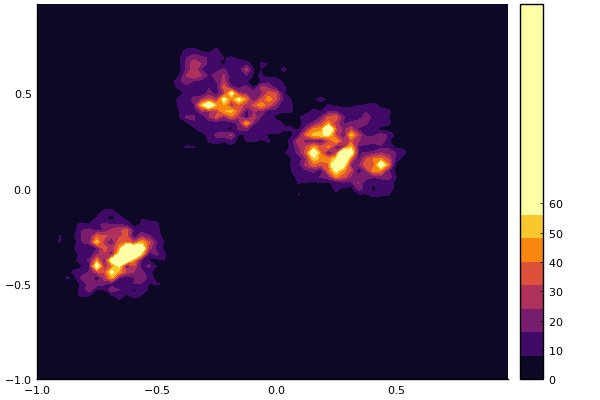
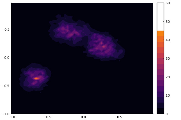
Figure 1: Energy density (legend on the right side of each subplot, in GeV⁴) produced in a pA collision in one event, represented in the transverse plane (coordinates measured in fm) for two values of $\tau$: upper panel corresponds to $\tau=0.002$ fm/c, lower panel to $\tau=0.15$ fm/c.

In Figure 1 we plot the energy density for a pA collision at two different times. In the upper panel, which represents the energy density right after the collision ($\tau=0.002$ fm/c), we notice the energy density concentrated over the three lumps standing for the three constituent quarks in the proton. In the lower panel, we plot $\varepsilon$ for $\tau=0.15$ fm/c. We notice that the expansion in the transverse plane is negligible, while the energy density is diluted due to the longitudinal expansion of the system.

For completeness, in Fig. 2 we plot $\varepsilon$ versus $\tau$ for both pA and AA collisions, averaged over $50$ events and over the transverse plane. In order to perform the transverse plane average consistently in the pA case, we have used the thickness function of the proton $T_{p}(\mathbf{x}_{\perp})$ as a weight, i.e. we plot $\langle\langle\text{Tr}[E_{L}^{2}+B_{L}^{2}+E_{T}^{2}+B_{T}^{2}]\rangle\rangle$ where $\langle\langle\cdot\rangle\rangle$ is defined as in (33). The results have been obtained for a square grid of transverse size $L=2$ fm, with $32\times 32$ lattice points. We notice that the free-streaming regime, $\varepsilon\sim 1/\tau$, sets in at $\tau\approx 0.1$ fm/c. For reference, the initial values of $\varepsilon$ are, expressed in terms of energy over volume, around 240 GeV/fm³ for pA and 960 GeV/fm³ for AA.

Figure 2: Energy density, $\varepsilon$, versus proper time. In both the pA and AA cases $\varepsilon$ has been averaged over $50$ events and over the transverse plane (the latter average has been performed using $T_{p}(\mathbf{x}_{\perp})$ as a weight, see main text).

III Quarks of infinite mass in glasma

Next we turn to the diffusion of HQs in the evolving glasma fields. This problem has attracted a lot of interest recently, see for example [50, 51, 52, 53, 54, 55, 56, 57, 58, 59, 60, 16, 61] as well as references therein. So far, this problem has been solved using a classical approximation in which the equations of motion for the HQs are the Wong equations  [62, 63]. In this work, we limit ourselves to analyze the diffusion of heavy quarks in the very-large mass limit, similarly to what has been done in [44].

One of the quantities we want to study is the momentum broadening, $\delta p_{i}^{2}$, of the HQs. This is defined as

$$\delta p_{i}^{2}(\tau)\equiv p_{i}^{2}(\tau)-p_{i}^{2}(\tau_{\text{form}}),~~~i=x,y,z,$$ (28)

where $\tau_{\text{form}}$ is the formation time of the HQ and $p^{i}(\tau_{\text{form}})$ the $i$-th component of the momentum at the formation time. In order to compute the momentum broadening, we need to specify the initial distribution of the HQs in the configuration space. To this end, we assume that HQs are produced near the hotspots of the energy density, see Fig. 1. Hence, it is reasonable to distribute the HQs according to the $T_{p}(\mathbf{x}_{\perp})$ in Eq. (5). Following the same arguments presented in [15], from the Wong equations we can write the momentum broadening of each heavy quark, in the $M\rightarrow\infty$ limit, as

$$\delta p_{L}^{2}(\tau) = g^{2}\int_{0}^{\tau}d\tau^{\prime}\int_{0}^{\tau}d\tau^{\prime\prime}\text{Tr}[E_{z}(\tau^{\prime})E_{z}(\tau^{\prime\prime})],$$ (29)

$$\delta p_{T}^{2}(\tau) = g^{2}\int_{0}^{\tau}d\tau^{\prime}\int_{0}^{\tau}d\tau^{\prime\prime}\frac{1}{\tau^{\prime}\tau^{\prime\prime}}\text{Tr}[E_{x}(\tau^{\prime})E_{x}(\tau^{\prime\prime})+E_{y}(\tau^{\prime})E_{y}(\tau^{\prime\prime})],$$ (30)

where we took the formation time of the infinitely massive HQs equal to zero, since $\tau_{\text{form}}=O(1/M)$ and $M\to\infty$. The integrands in the left-hand side of Eqs. (29) and (30) depend also on the transverse plane coordinates. Integrating over the whole transverse plane and ensemble-averaging Eqs. (29) and (30), results in

$$\langle\langle\delta p_{L}^{2}(\tau)\rangle\rangle = g^{2}\int_{0}^{\tau}d\tau^{\prime}\int_{0}^{\tau}d\tau^{\prime\prime}\int d^{2}\mathbf{x}_{\perp}\langle\text{Tr}[E_{z}(\tau^{\prime})E_{z}(\tau^{\prime\prime})]T_{p}(\mathbf{x}_{\perp})\rangle,$$ (31)

$$\langle\langle\delta p_{T}^{2}(\tau)\rangle\rangle = g^{2}\int_{0}^{\tau}d\tau^{\prime}\int_{0}^{\tau}d\tau^{\prime\prime}\int d^{2}\mathbf{x}_{\perp}\frac{1}{\tau^{\prime}\tau^{\prime\prime}}\langle\text{Tr}[E_{x}(\tau^{\prime})E_{x}(\tau^{\prime\prime})+E_{y}(\tau^{\prime})E_{y}(\tau^{\prime\prime})]T_{p}(\mathbf{x}_{\perp})\rangle,$$ (32)

where $T_{p}(\mathbf{x}_{\perp})$ is defined in Eq. (5) and takes into account the initial distribution of the HQs in the configuration space. The symbol $\langle\rangle$ denotes the ensemble average, while

$$\langle\langle\delta p_{L,T}^{2}(\tau)\rangle\rangle=\int d^{2}\mathbf{x}_{\perp}\langle\delta p_{L,T}^{2}(\tau)T_{p}(\mathbf{x}_{\perp})\rangle.$$ (33)

In writing Eqs. (31) and (32) we took advantage of the fact that the HQs are infinitely massive, therefore their distribution in the configuration space does not change in time.

The equations (31) and (32) are formally similar to what we would obtain in the case of a standard Langevin equation for a purely diffusive motion: $dp^{i}/dt=\xi^{i}$, where $\xi^{i}$ denotes the random force. In fact, in this case we would obtain [55]

$$\langle\delta p_{i}^{2}\rangle=\int_{0}^{t}dt_{1}\int_{0}^{t}dt_{2}\langle\xi_{i}(t_{1})\xi_{i}(t_{2})\rangle.$$ (34)

We can indeed notice the similarity among (34) and Eqs. (31) and (32) after realizing that the role of the random force in the context of HQs is taken by the force exerted by the color-electric field. We also notice that in the infinite mass limit Eqs. (31) and (32) are exact, in the sense that the color-magnetic field gives no contribution in this limit as its effect is proportional to the velocity of the quarks, which vanishes for $M\to\infty$. For $i=x,y$ the resulting equation for the momenta shift can be evaluated directly from the $E_{x}$ and $E_{y}$ fields. On the other hand, in principle we need to explicitly compute the $E_{z}$ component of the color-electric field from the $(\tau,\eta)$ components. This can be easily achieved as under the change of coordinates from $x^{\mu^{\prime}}=(\tau,\eta)$ to $x^{\mu}=(t,z)$ in Eq. (1) we have

$$E_{z}=F_{0z}=\frac{\partial x^{\mu^{\prime}}}{\partial t}\frac{\partial x^{\nu^{\prime}}}{\partial z}F_{\mu\nu}^{{}^{\prime}}=F_{\tau\eta}=E_{\eta}.$$ (35)

Consequently, the knowledge of the $\eta-$component of the field, which we easily extract from the Yang-Mills equations, is enough to compute the momentum spreading along the $z$ direction.

III.1 Momentum and angular momentum broadening

Figure 3: Longitudinal momentum broadening, $\langle\delta p_{L}^{2}(\tau)\rangle$, and transverse momentum broadening, $\langle\delta p_{T}^{2}(\tau)\rangle$, for a pA collision. Calculations correspond to an average over $100$ events, for a transverse plane with $32\times 32$ points and transverse size $L=2$ fm. The orange line corresponds to the function $a+b\log(\tau/\bar{\tau})$ where we put $\bar{\tau}=0.4$ fm/c, $a=0.92$ GeV² and $b=0.2$ GeV², obtained via a best-fit procedure of the data obtained for $\langle\delta p_{L}^{2}(\tau)\rangle$. Similarly, the green solid line represents the function $c+d\log(\tau/\tilde{\tau})$ where we put $\tilde{\tau}=0.2$ fm/c, $c=0.29$ GeV² and $d=0.01$ GeV², obtained via a best-fit procedure of the data obtained for $\langle\delta p_{T}^{2}(\tau)\rangle$.

One of the things most studied in the context of HQs in the pre-equilibrium stage of pA and AA collisions is the momentum broadening, see for example [50, 51, 52, 53, 54, 55, 56, 57, 58, 59, 60, 16, 61]. We analyze this quantity in the present study, bringing the novelty of introducing longitudinal fluctuations. As a benchmark, we firstly show the results obtained without fluctuations.

In Fig. 3 we show $\langle\delta p_{L}^{2}(\tau)\rangle$ and $\langle\delta p_{T}^{2}(\tau)\rangle$ versus proper time. The evolution is shown up to $\tau=0.7$ fm/c for the sake of illustration: it is likely that in real pA collisions the pre-equilibrium stage lasts for a short fraction of fm/c only, hence our results are phenomenologically relevant up to $\tau\approx 0.5$ fm/c at most. We notice that the transverse momentum shift is substantially lower than the longitudinal one: this is a consequence of the predominance of the longitudinal color-electric fields in the first instants after the collision. The anisotropy of the evolving glasma, which reflects onto the difference between the longitudinal and the transverse field correlators, is transmitted to the momentum broadenings. We find that, as a result of the diffusion of the HQs in the evolving glasma fields, both $\langle\delta p_{L}^{2}(\tau)\rangle$ and $\langle\delta p_{T}^{2}(\tau)\rangle$ grow up with proper time; after a short transient lasting up to $\tau\approx 0.5$ fm/c, the growth of $\langle\delta p_{T}^{2}(\tau)\rangle$ drastically slows down, while that of $\langle\delta p_{L}^{2}(\tau)\rangle$ remains substantial for the whole time range considered here. The values obtained can be compared, for example, with those found in [15] for AA collisions: our momenta shifts are smaller since we are dealing with pA collisions, in which the charge density (and hence the energy density) is smaller.

The late-time behavior of $\langle\delta p_{L}^{2}(\tau)\rangle$ and $\langle\delta p_{T}^{2}(\tau)\rangle$ can be interpreted by assuming a $\delta-$like correlator of the color-electric fields. For instance, let us assume that for $E_{z}$ we have

$$\langle E_{z}(\tau^{\prime})E_{z}(\tau^{\prime\prime})\rangle=\frac{\langle E_{z}^{2}(\tau^{\prime})\rangle}{Q_{s}}\delta(\tau^{\prime}-\tau^{\prime\prime}),$$ (36)

where the overall $1/Q_{s}$ on the right hand side of the above equation is added in order to balance the units of the $\delta$ function. The particular choice of $Q_{s}$ in the equation is due to the fact that $Q_{s}$ is the only energy scale in the MV model. Using the ansatz (36) in Eq. (31) we easily get

$$\langle\delta p_{L}^{2}(\tau)\rangle_{M\to\infty}\approx g^{2}Q_{s}^{-1}\int_{\bar{\tau}}^{\tau}d\tau^{\prime}\langle E_{z}^{2}(\tau^{\prime})\rangle,$$ (37)

where we cut the time-integral down to $\bar{\tau}$, which represents a value of the proper time of the order of $1/Q_{s}$. We introduce it since we are interested in the late-time behavior only, indeed it is large enough that allows us to use $\langle E_{z}^{2}(\tau^{\prime})\rangle\propto Q_{s}^{4}/(Q_{s}\tau^{\prime})$, in agreement with the late-time behavior of the energy density, see Fig. 2. We have also inserted the needed powers of $Q_{s}$ in order to get the correct dimension of energy to the fourth power. We thus get

$$\langle\delta p_{L}^{2}(\tau)\rangle_{M\to\infty}\propto g^{2}Q_{s}^{2}\log(\tau/\bar{\tau}),~~~\text{for }\tau/\bar{\tau}>1.$$ (38)

The behavior (38) of $\langle\delta p_{L}^{2}(\tau)\rangle$ (and similar calculation hold for $\langle\delta p_{T}^{2}(\tau)\rangle$) is in fair agreement with the results of the full numerical simulations, see Fig. 3. As a final comment on the results shown in Fig. 3, we notice that we measure some tiny fluctuations of both $\langle\delta p_{L}^{2}(\tau)\rangle$ and $\langle\delta p_{T}^{2}(\tau)\rangle$, similarly to what observed in [15]. The amplitude of these fluctuations is however very small in comparison with the bulk value of these quantities, thus they are practically irrelevant.

The momentum anisotropy is also transmitted to other observables of the HQs. In particular, one can look at the angular momentum anisotropy parameter, $\Delta_{2}$, defined as [58]

$$\Delta_{2}\equiv\frac{\langle L_{x}^{2}-L_{z}^{2}\rangle}{\langle L_{x}^{2}+L_{z}^{2}\rangle},$$ (39)

where $L_{i}$, with $i=x,y,z$, denotes the $i^{th}$ component of the orbital angular momentum of the HQ. $\Delta_{2}$ therefore measures the anisotropy of the fluctuations of the orbital angular momentum of the HQs. It is also worth noting that $\Delta_{2}$ receives contribution from both the anisotropy of the color fields and from the geometry of the system [58].

Such quantity can be rewritten in terms of the averages of the squared components of the momentum of the HQs. This can be done following the same steps given in [58] and assuming that momenta and positions of the HQs are not correlated with each other. We have

$$\langle L_{x}^{2}\rangle =\langle(yp_{z}-zp_{y})^{2}\rangle\simeq\langle y^{2}\rangle\langle p_{z}^{2}\rangle+\langle z^{2}\rangle\langle p_{y}^{2}\rangle,$$

$$\langle L_{z}^{2}\rangle =\langle(xp_{y}-yp_{x})^{2}\rangle\simeq\langle x^{2}\rangle\langle p_{y}^{2}\rangle+\langle y^{2}\rangle\langle p_{x}^{2}\rangle.$$ (40)

The above expressions allow us to write

$$\Delta_{2}=\frac{[\langle z^{2}\rangle-\langle x^{2}\rangle-\langle y^{2}\rangle]\langle p_{T}^{2}\rangle/2+\langle y^{2}\rangle\langle p_{z}^{2}\rangle}{[\langle z^{2}\rangle+\langle x^{2}\rangle+\langle y^{2}\rangle]\langle p_{T}^{2}\rangle/2+\langle y^{2}\rangle\langle p_{z}^{2}\rangle}.$$ (41)

This expression can be further specialized to the case of a pA collision as follows. Firstly, we estimate the mean squared value of the longitudinal $\langle z^{2}\rangle$ and of the transverse coordinates $\langle x^{2}\rangle$ and $\langle y^{2}\rangle$. As far as the extension along the beam axis $z$ is concerned, we will assume that the HQs are generated uniformly along the whole $\eta$ interval. This means that $\langle z^{2}\rangle$ will be given by:

$$\langle z^{2}\rangle=\frac{\displaystyle{\int_{-L_{\eta}/2}^{L_{\eta}/2}}d\eta\,(\tau\sinh\eta)^{2}}{\displaystyle{\int_{-L_{\eta}/2}^{L_{\eta}/2}}d\eta}=\frac{1}{2}\tau^{2}\left(\frac{\sinh L_{\eta}}{L_{\eta}}-1\right).$$ (42)

We fix the $\eta$ extension as $L_{\eta}=2$, corresponding to the rapidity range $[-1,1]$. For what concerns the transverse coordinates, firstly we assume that the geometrical distribution of the HQs in the transverse plane follows the same profile of the initial energy density, which in turn resembles that of the color charges of the colliding proton. This is a fair approximation considering that most HQs will be produced by hard QCD scatterings where the density of the color charges is larger, as well as the fact that the transverse expansion is not so important in the pre-equilibrium stage, see for example Fig. 1. Within these reasonable approximations, we can estimate $\langle\mathbf{x}_{\perp}^{2}\rangle=\langle x^{2}+y^{2}\rangle$. Firstly, we fix the location of the three constituent quarks, $\mathbf{x}_{i}$, and we average over the transverse coordinates using the thickness function $T_{p}(\mathbf{x}_{\perp})$ in (5), getting

$$\langle\mathbf{x}_{\perp}^{2}\rangle_{\mathbf{x}_{i}}=\frac{\displaystyle{\int}d^{2}\mathbf{x}_{\perp}\,\mathbf{x}_{\perp}^{2}\,T_{p}(\mathbf{x}_{\perp})}{\displaystyle{\int}d^{2}\mathbf{x}_{\perp}\,T_{p}(\mathbf{x}_{\perp})}=2B_{q}+\frac{1}{3}\sum_{i=1}^{3}\mathbf{x}_{i}^{2}.$$ (43)

Then an average over the locations of the constituent quarks, $\mathbf{x}_{i}$, is needed: we perform this using the distribution $T_{cq}(\mathbf{x}_{i})$ in (6), resulting in

$$\langle\mathbf{x}_{\perp}^{2}\rangle=\frac{\displaystyle{\int}d^{2}\mathbf{x}_{i}\,\langle\mathbf{x}_{\perp}^{2}\rangle_{\mathbf{x}_{i}}T_{cq}(\mathbf{x}_{i})}{\displaystyle{\int}d^{2}\mathbf{x}_{i}\,T_{cq}(\mathbf{x}_{i})}=2B_{q}+2B_{cq}.$$ (44)

Hence,

$$\langle x^{2}\rangle=\langle y^{2}\rangle=\frac{1}{2}\langle\mathbf{x}_{\perp}^{2}\rangle=B_{q}+B_{cq}.$$ (45)

Using the results (42) and (45) in Eq. (41), along with the momenta shifts we previously got from (31) and (32), we can compute $\Delta_{2}$ for a pA collision.

As mentioned, a nonzero $\Delta_{2}$ is not only due to the anisotropy of the fields (which is reflected on a anisotropic momentum distribution), but entails a geometric contribution as well. The latter is related to the shape of the fireball and could be nonzero also in case momenta are isotropic. In order to extract the geometric contribution to $\Delta_{2}$, we start with Eq. (41) in which we evaluate $\langle p_{z}^{2}\rangle$ as follows. Since we have

$$p_{z}=p_{T}\sinh y\simeq p_{T}\sinh\eta,$$ (46)

by assuming once again that the HQs are uniformly spread in $\eta$ we have:

$$\langle p_{z}^{2}\rangle=\frac{\displaystyle{\int_{-L_{\eta}/2}^{L_{\eta}/2}}d\eta\,\langle p_{T}^{2}\rangle(\sinh\eta)^{2}}{\displaystyle{\int_{-L_{\eta}/2}^{L_{\eta}/2}}d\eta}=\frac{1}{2}\langle p_{T}^{2}\rangle\left(\frac{\sinh L_{\eta}}{L_{\eta}}-1\right).$$ (47)

This allows us to define the geometric component of $\Delta_{2}$, we call it $\Delta_{2}^{\text{geom}}$, namely

$$\Delta_{2}^{\text{geom}}=\frac{\langle z^{2}\rangle+\langle x^{2}\rangle-\langle y^{2}\rangle+\langle y^{2}\rangle\left(\sinh L_{\eta}/L_{\eta}-1\right)}{\langle z^{2}\rangle+\langle x^{2}\rangle+\langle y^{2}\rangle+\langle y^{2}\rangle\left(\sinh L_{\eta}/L_{\eta}-1\right)}=$$

$$=\frac{[\frac{1}{2}\tau^{2}+(B_{q}+B_{cq})]\left(\sinh L_{\eta}/L_{\eta}-1\right)}{[\frac{1}{2}\tau^{2}+(B_{q}+B_{cq})]\left(\sinh L_{\eta}/L_{\eta}-1\right)+2(B_{q}+B_{cq})}.$$ (48)

In Figure 4 we show our results for both $\Delta_{2}$ and $\Delta_{2}-\Delta_{2}^{\text{geom}}$. The calculations correspond to a pA collision for a $32\times 32\times 32$ lattice and an average over $50$ events. From Eq. (48) we get $\Delta_{2}^{\text{geom}}(\tau=0)=(\sinh L_{\eta}/L_{\eta}-1)/(\sinh L_{\eta}/L_{\eta}+1)\simeq 0.289$, therefore we have a geometric correction already at initial time. Notice also that $\Delta_{2}^{\text{geom}}(\tau=0)$ is independent with respect to the widths of the proton charge, namely $B_{q}$ and $B_{cq}$. For times up to $\tau\sim 0.15$ fm/c, $\Delta_{2}^{\text{geom}}(\tau)$ varies with time but quite slowly (see the $\tau^{2}$ term in (48)), hence $\Delta_{2}^{\text{geom}}(\tau)\simeq\Delta_{2}^{\text{geom}}(\tau=0)$ and the two curves in Figure 4 differ basically by a constant. During this time we observe most of the damping for both curves. For even larger times we see that $\Delta_{2}$ shows an increasing behavior, but a look at $\Delta_{2}-\Delta_{2}^{\text{geom}}$ in the same time scales shows that the increase in angular momentum anisotropy is likely due to an expansion of the system, mostly along the longitudinal direction. Indeed, by subtracting the geometric component we see that the pure anisotropy of the glasma fields (blue dashed curve) decreases with time.

Figure 4: $\Delta_{2}$ (full black) and $\Delta_{2}-\Delta_{2}^{\text{geom}}$ (dashed blue) versus proper time for pA collisions.

IV Inclusion of field fluctuations

As already explained in the Introduction, in relativistic nuclear collisions one clearly does not have exact boost-invariance. In particular, the glasma is the solution of the Yang-Mills equations only in the case of weak coupling $g$: for realistic values of $g$ it is likely that quantum fluctuations develop, with a strength that increases with $g$. For instance, in [24] it has been shown that increasing $g$ leads to a larger contribution of fluctuations to the longitudinal pressures. Since a finite value of $g$ is relevant for realistic collisions, it is meaningful to repeat the analysis presented in the previous section to the case in which we add fluctuations on top of the glasma. We construct the fluctuations by adding terms to the boost-invariant electric fields at initial time. These additions satisfy the Gauss’ law

$$D_{i}E_{i}+D_{\eta}E_{\eta}=0.$$ (49)

Firstly, we evaluate random configurations $\xi_{i}(\mathbf{x}_{\perp})$ ($i=x,y$) such that

$$\langle\xi_{i}(\mathbf{x}_{\perp})\xi_{j}(\mathbf{y}_{\perp})\rangle=\delta_{ij}\delta^{(2)}(\mathbf{x}_{\perp}-\mathbf{y}_{\perp}),$$ (50)

which are operatively generated by sampling random Gaussian numbers with zero average and standard deviation $1/a_{\perp}$. After that, the additional terms to the glasma color-electric fields are evaluated as [22, 21]

$$\delta E^{i}(\mathbf{x}_{\perp},\eta)=-\partial_{\eta}F(\eta)\xi_{i}(\mathbf{x}_{\perp}),$$ (51)

$$\delta E^{\eta}(\mathbf{x}_{\perp},\eta)=F(\eta)\sum_{i=x,y}D_{i}\xi_{i}(\mathbf{x}_{\perp}).$$ (52)

The information about the $\eta-$distribution of the fluctuations is encoded in the function $F(\eta)$. By construction, these fluctuations satisfy the Gauss law constraint (49). The above relations are discretized on the lattice as [22]

$$\delta E^{i}(\mathbf{x}_{\perp},\eta)=a_{\eta}^{-1}[F(\eta-a_{\eta})-F(\eta)]\xi_{i}(\mathbf{x}_{\perp}),$$ (53)

$$\delta E^{\eta}(\mathbf{x}_{\perp},\eta)=-a_{\perp}^{-1}F(\eta)\sum_{i=x,y}[\Xi^{i}(\mathbf{x}_{\perp})-\xi^{i}(\mathbf{x}_{\perp})],$$ (54)

where

$$\Xi^{i}(\mathbf{x}_{\perp})=U_{i}^{\dagger}(\mathbf{x}_{\perp}-\hat{i})\xi_{i}(\mathbf{x}_{\perp}-\hat{i})U_{i}(\mathbf{x}_{\perp}-\hat{i}).$$ (55)

In the above equations, $a_{\eta}=L_{\eta}/N_{\eta}$ is the lattice spacing along the $\eta$ direction. The term $\Xi^{i}(\mathbf{x}_{\perp})-\xi^{i}(\mathbf{x}_{\perp})$ is the covariant derivative of $\xi^{i}$, expressed in terms of the gauge links. Moreover, also in the longitudinal direction, periodic boundary conditions have been implemented for points at the edge of the $\eta$ domain. As far as the choice of the rapidity-dependent term $F(\eta)$ is concerned, one may consider different approaches. For instance, in [21] the authors implemented a model in which $F(\eta)$ is a Gaussian random number with zero mean and standard deviation equal to one. In this work, we instead follow a simpler model of fluctuations, similar to the one introduced in [22], in which $F(\eta)$ takes the form

$$F(\eta)=\frac{\Delta}{N_{\perp}}\sum_{n\in\mathcal{I}}\frac{1}{|\mathcal{I}|}\cos\left(\frac{2\pi n\eta}{L_{\eta}}\right),$$ (56)

where $\mathcal{I}\in\mathbb{N}$ denotes a set of positive integers with cardinality $|\mathcal{I}|$; the higher the order of the harmonics that contribute to $F(\eta)$ in (56) the higher the energy carried by the transverse fields of the fluctuations, see the $\eta$-derivative in Eq. (51).

IV.1 Momentum broadening fluctuations

In this subsection we present our results on the impact of the initial fluctuations on the momentum broadening of the HQs in the pre-equilibrium stage of pA collisions. The fluctuations are added on top of the boost-invariant glasma at $\tau\equiv\tau_{0}=0.05$ fm/c; we checked that the results are not significantly affected by changing $\tau_{0}$ in the range $[0.01,0.05]$ fm/c.

Figure 5: The ratio of the longitudinal pressure over the transverse pressure $P_{L}/P_{T}$, versus proper time for different values of $\Delta$ (including the boost invariant $\Delta=0$ case, black line).

Figure 6: The longitudinal and transverse momentums shifts, $\langle\delta p_{L}^{2}(\tau)\rangle$ and $\langle\delta p_{T}^{2}(\tau)\rangle$, versus proper time for different values of $\Delta$ (including the boost invariant $\Delta=0$ case, black line). We used $\mathcal{I}=\{1,\dots,10\}$ in Eq. (56).

In Fig. 5 we show, for the set of harmonics $\mathcal{I}=\{1,\dots,10\}$ and several values of $\Delta$, the ratio of longitudinal pressure over transverse pressure, $P_{L}/P_{T}$, versus proper time. These quantities are defined as [22]:

$$P_{L} =\langle\langle\text{Tr}[E_{T}^{2}+B_{T}^{2}-E_{L}^{2}-B_{L}^{2}]\rangle\rangle.$$ (57)

$$P_{T} =\langle\langle\text{Tr}[E_{L}^{2}+B_{L}^{2}]\rangle\rangle.$$ (58)

where the ensemble average is performed as in (33). The main purpose of the results shown in Fig. 5 is to highlight the net effect of the fluctuations on the bulk gluon fields. Indeed, for the highest value of $\Delta$, we find a non-trivial behavior of $P_{L}/P_{T}$, which is quite different from the one we find for smaller values of $\Delta$ as well as $\Delta=0$. In particular, $P_{L}/P_{T}$ stays of order one within the early stage. We remark that the largest value of $\Delta$ used in Fig. 5, that is $\Delta=0.5$, is probably too large as it corresponds to have a system whose energy is carried half by glasma and half by fluctuations. Nevertheless, it is shown to illustrate that fluctuations are actually introduced in the bulk and substantially modify it.

Next, we turn to the momentum broadening. In Fig. 6 we plot $\langle\langle\delta p_{L}^{2}(\tau)\rangle\rangle$ and $\langle\langle\delta p_{T}^{2}(\tau)\rangle\rangle$ versus proper time. We show results for the same set of harmonics $\mathcal{I}=\{1,\dots,10\}$ and for the same parameters $\Delta$ we have already considered in Fig. 5. Along with the event averages, for the non-boost invariant curves we also plot the statistical uncertainty as an error band, obtained as the standard deviation of the mean value: $\sigma_{\text{avg}}=\sigma/\sqrt{N_{\text{events}}-1}$. For the $\Delta=0$ curve the error bars are not shown for clarity but we checked they overlap with the ones shown in the figure. In addition to the averaging over the transverse plane (as in (33)), we average on the space-time rapidity of the HQs, restricting ourselves to the rapidity range $[-1,1]$. We find no net effect of the rapidity fluctuations on the momenta shifts, since the $\Delta=0$ (black curve) result lies within the error bars of all the other $\Delta\neq 0$ data, including the highest value $\Delta=0.5$.

Our conclusion is that the fluctuations do not affect substantially the HQ momenta shifts in the static limit. Our interpretation is that momentum broadening is related, in the static limit, to the time-correlator of the color-electric fields, see Eqs. (31) and (32), and these correlators are not very much affected by the longitudinal fluctuations, which add a non-trivial dependence of the fields on $\eta$ and mostly modify correlations along the $\eta$-direction [64].

V Conclusions

We studied the diffusion of heavy quarks in the early stage of high-energy proton-nucleus collisions. Our initial condition is based on the glasma picture, and includes event-by-event fluctuations of the color charges in the proton, as well as fluctuations that break the boost invariance. We performed $3+1$D real-time statistical simulations of the $SU(3)$ Yang-Mills fields produced immediately after the collision. Both the modeling of the proton and the longitudinal fluctuations for an expanding geometry in $SU(3)$ have not been considered before in the literature in the context of heavy quarks. For simplicity, we limited ourselves to study the large-mass limit of the heavy quarks: in this limit, the solution of the Wong equations for the momentum diffusion amounts to computing the time-correlator of the color-electric fields. As a model of initial state field fluctuations, we adopted a simple superposition of several harmonics [22], with a free parameter, $\Delta$, that measures the strength of the fluctuating fields, see Eq. (56). The fact that the strength of the fluctuating fields scales as $\Delta/|\mathcal{I}|$ in Eq. (56) allows us to keep the initial energy density carried by the fluctuations unaffected by the inclusion of more harmonics.

We found that momentum broadening both in longitudinal direction and in the transverse plane, $\langle\delta p_{L}^{2}\rangle$ and $\langle\delta p_{T}^{2}\rangle$ respectively, are unaffected (within error bars) by the inclusion of $\eta$-dependent fluctuations. Our interpretation of this result is that the fluctuations do not alter in a substantial way the time correlations of the color-electric fields, that are directly related to momentum broadening. Hence, our conclusion is that the initial state fluctuations, at least in the form introduced within our study, might be not sufficient to achieve isotropization of heavy quark momenta within the early stage. This occurs despite the fact that for the (illustrative) case of intense fluctuations considered in our work, the quantity $P_{L}/P_{T}$, which is a measure of the amount of anisotropy of the bulk gluon fields, stays of order one.

Additionally, we computed the anisotropy of the angular momentum fluctuations, that we quantified by the coefficient $\Delta_{2}$ introduced in [58]. In [58] the $\Delta_{2}$ has been studied for a static geometry, within the gauge group $SU(2)$ and without initial state fluctuations, hence the present work improves these several aspects with respect to [58]. We found that $\Delta_{2}$ remains considerably large during the whole early stage: in the time range where the picture based on an evolving glasma is phenomenologically relevant, that is for $\tau$ in the range $[0.2,0.4]$ fm/c, $\Delta_{2}$ remains in the range $[0.4,0.6]$, signaling a substantial amount of anisotropic angular momentum fluctuations. For larger times we can grasp a linear trend for $\Delta_{2}$, however such behavior not only may not be accessible phenomenologically, but it is also likely due to the expansion of the system, rather than a genuine feature of the glasma fields.

The work we presented here can be improved in several ways. Certainly, the most important improvement would be the inclusion of dynamical heavy quarks, hence going beyond the large-mass limit. That should be accompanied by a proper initialization of the heavy quarks in momentum space, as already done in [65]. These improvements will be presented in the near future.

Acknowledgments

M. R. acknowledges Francesco Acerbi and John Petrucci for inspiration. The authors acknowledge numerous discussions with Dana Avramescu, Bjorn Schenke and Raju Venugopalan. This work has been partly funded by the European Union – Next Generation EU through the research grant number P2022Z4P4B “SOPHYA - Sustainable Optimised PHYsics Algorithms: fundamental physics to build an advanced society” under the program PRIN 2022 PNRR of the Italian Ministero dell’Università e Ricerca (MUR).

References

- Heinz and Jacob [2000] U. W. Heinz and M. Jacob, Evidence for a new state of matter: An Assessment of the results from the CERN lead beam program, (2000), arXiv:nucl-th/0002042 .
- Heinz and Snellings [2013] U. Heinz and R. Snellings, Collective flow and viscosity in relativistic heavy-ion collisions, Ann. Rev. Nucl. Part. Sci. 63, 123 (2013), arXiv:1301.2826 [nucl-th] .
- Harris and Muller [1996] J. W. Harris and B. Muller, The Search for the quark - gluon plasma, Ann. Rev. Nucl. Part. Sci. 46, 71 (1996), arXiv:hep-ph/9602235 .
- Schenke et al. [2012a] B. Schenke, P. Tribedy, and R. Venugopalan, Event-by-event gluon multiplicity, energy density, and eccentricities in ultrarelativistic heavy-ion collisions, Phys. Rev. C 86, 034908 (2012a), arXiv:1206.6805 [hep-ph] .
- Schenke et al. [2012b] B. Schenke, P. Tribedy, and R. Venugopalan, Fluctuating Glasma initial conditions and flow in heavy ion collisions, Phys. Rev. Lett. 108, 252301 (2012b), arXiv:1202.6646 [nucl-th] .
- McLerran and Venugopalan [1994a] L. D. McLerran and R. Venugopalan, Computing quark and gluon distribution functions for very large nuclei, Phys. Rev. D 49, 2233 (1994a), arXiv:hep-ph/9309289 .
- McLerran and Venugopalan [1994b] L. D. McLerran and R. Venugopalan, Gluon distribution functions for very large nuclei at small transverse momentum, Phys. Rev. D 49, 3352 (1994b), arXiv:hep-ph/9311205 .
- McLerran and Venugopalan [1994c] L. D. McLerran and R. Venugopalan, Green’s functions in the color field of a large nucleus, Phys. Rev. D 50, 2225 (1994c), arXiv:hep-ph/9402335 .
- Gelis et al. [2010] F. Gelis, E. Iancu, J. Jalilian-Marian, and R. Venugopalan, The Color Glass Condensate, Ann. Rev. Nucl. Part. Sci. 60, 463 (2010), arXiv:1002.0333 [hep-ph] .
- Iancu and Venugopalan [2003] E. Iancu and R. Venugopalan, The Color glass condensate and high-energy scattering in QCD, in Quark-gluon plasma 4, edited by R. C. Hwa and X.-N. Wang (2003) pp. 249–3363, arXiv:hep-ph/0303204 .
- McLerran [2009] L. McLerran, A Brief Introduction to the Color Glass Condensate and the Glasma, in 38th International Symposium on Multiparticle Dynamics (2009) pp. 3–18, arXiv:0812.4989 [hep-ph] .
- Gelis [2013] F. Gelis, Color Glass Condensate and Glasma, Int. J. Mod. Phys. A 28, 1330001 (2013), arXiv:1211.3327 [hep-ph] .
- Carrington et al. [2022a] M. E. Carrington, A. Czajka, and S. Mrowczynski, The energy-momentum tensor at the earliest stage of relativistic heavy-ion collisions, Eur. Phys. J. A 58, 5 (2022a), arXiv:2012.03042 [hep-ph] .
- Carrington et al. [2022b] M. E. Carrington, A. Czajka, and S. Mrówczyński, Physical characteristics of glasma from the earliest stage of relativistic heavy ion collisions, Phys. Rev. C 106, 034904 (2022b), arXiv:2105.05327 [hep-ph] .
- Avramescu et al. [2023] D. Avramescu, V. Băran, V. Greco, A. Ipp, D. I. Müller, and M. Ruggieri, Simulating jets and heavy quarks in the glasma using the colored particle-in-cell method, Phys. Rev. D 107, 114021 (2023), arXiv:2303.05599 [hep-ph] .
- Avramescu et al. [2024a] D. Avramescu, V. Greco, T. Lappi, H. Mäntysaari, and D. Müller, The impact of glasma on heavy flavor azimuthal correlations and spectra, (2024a), arXiv:2409.10564 [hep-ph] .
- Pang et al. [2013] L. Pang, Q. Wang, and X.-N. Wang, Effect of longitudinal fluctuation in event-by-event (3+1)D hydrodynamics, Nucl. Phys. A 904-905, 811c (2013), arXiv:1211.1570 [nucl-th] .
- Pang et al. [2015] L.-G. Pang, G.-Y. Qin, V. Roy, X.-N. Wang, and G.-L. Ma, Longitudinal decorrelation of anisotropic flows in heavy-ion collisions at the CERN Large Hadron Collider, Phys. Rev. C 91, 044904 (2015), arXiv:1410.8690 [nucl-th] .
- Fukushima [2014] K. Fukushima, Turbulent pattern formation and diffusion in the early-time dynamics in relativistic heavy-ion collisions, Phys. Rev. C 89, 024907 (2014), arXiv:1307.1046 [hep-ph] .
- Romatschke and Venugopalan [2006a] P. Romatschke and R. Venugopalan, Collective non-Abelian instabilities in a melting color glass condensate, Phys. Rev. Lett. 96, 062302 (2006a), arXiv:hep-ph/0510121 .
- Romatschke and Venugopalan [2006b] P. Romatschke and R. Venugopalan, The Unstable Glasma, Phys. Rev. D 74, 045011 (2006b), arXiv:hep-ph/0605045 .
- Fukushima and Gelis [2012] K. Fukushima and F. Gelis, The evolving Glasma, Nucl. Phys. A 874, 108 (2012), arXiv:1106.1396 [hep-ph] .
- Iida et al. [2014] H. Iida, T. Kunihiro, A. Ohnishi, and T. T. Takahashi, Time evolution of gluon coherent state and its von Neumann entropy in heavy-ion collisions, (2014), arXiv:1410.7309 [hep-ph] .
- Epelbaum and Gelis [2013a] T. Epelbaum and F. Gelis, Pressure isotropization in high energy heavy ion collisions, Phys. Rev. Lett. 111, 232301 (2013a), arXiv:1307.2214 [hep-ph] .
- Epelbaum and Gelis [2013b] T. Epelbaum and F. Gelis, Fluctuations of the initial color fields in high energy heavy ion collisions, Phys. Rev. D 88, 085015 (2013b), arXiv:1307.1765 [hep-ph] .
- Ryblewski and Florkowski [2013] R. Ryblewski and W. Florkowski, Equilibration of anisotropic quark-gluon plasma produced by decays of color flux tubes, Phys. Rev. D 88, 034028 (2013), arXiv:1307.0356 [hep-ph] .
- Ruggieri et al. [2015] M. Ruggieri, A. Puglisi, L. Oliva, S. Plumari, F. Scardina, and V. Greco, Modelling Early Stages of Relativistic Heavy Ion Collisions: Coupling Relativistic Transport Theory to Decaying Color-electric Flux Tubes, Phys. Rev. C 92, 064904 (2015), arXiv:1505.08081 [hep-ph] .
- Tanji and Itakura [2012] N. Tanji and K. Itakura, Schwinger mechanism enhanced by the Nielsen–Olesen instability, Phys. Lett. B 713, 117 (2012), arXiv:1111.6772 [hep-ph] .
- Berges and Schlichting [2013] J. Berges and S. Schlichting, The nonlinear glasma, Phys. Rev. D 87, 014026 (2013), arXiv:1209.0817 [hep-ph] .
- Berges et al. [2014a] J. Berges, K. Boguslavski, S. Schlichting, and R. Venugopalan, Universal attractor in a highly occupied non-Abelian plasma, Phys. Rev. D 89, 114007 (2014a), arXiv:1311.3005 [hep-ph] .
- Berges et al. [2014b] J. Berges, K. Boguslavski, S. Schlichting, and R. Venugopalan, Basin of attraction for turbulent thermalization and the range of validity of classical-statistical simulations, JHEP 05, 054, arXiv:1312.5216 [hep-ph] .
- Berges et al. [2014c] J. Berges, K. Boguslavski, S. Schlichting, and R. Venugopalan, Turbulent thermalization process in heavy-ion collisions at ultrarelativistic energies, Phys. Rev. D 89, 074011 (2014c), arXiv:1303.5650 [hep-ph] .
- Bazak and Mrowczynski [2024] S. Bazak and S. Mrowczynski, Stability of initial glasma fields, Phys. Rev. C 109, 024903 (2024), arXiv:2310.02205 [hep-ph] .
- Tsukiji et al. [2016] H. Tsukiji, H. Iida, T. Kunihiro, A. Ohnishi, and T. T. Takahashi, Entropy production from chaoticity in Yang-Mills field theory with use of the Husimi function, Phys. Rev. D 94, 091502 (2016), arXiv:1603.04622 [hep-ph] .
- Tsukiji et al. [2018] H. Tsukiji, T. Kunihiro, A. Ohnishi, and T. T. Takahashi, Entropy production and isotropization in Yang–Mills theory using a quantum distribution function, PTEP 2018, 013D02 (2018), arXiv:1709.00979 [hep-ph] .
- Matsuda et al. [2022] H. Matsuda, T. Kunihiro, A. Ohnishi, and T. T. Takahashi, Entropy production in a longitudinally expanding Yang–Mills field with use of the Husimi function: semiclassical approximation, PTEP 2022, 073D02 (2022), arXiv:2203.02859 [hep-ph] .
- Dusling et al. [2016] K. Dusling, W. Li, and B. Schenke, Novel collective phenomena in high-energy proton–proton and proton–nucleus collisions, Int. J. Mod. Phys. E 25, 1630002 (2016), arXiv:1509.07939 [nucl-ex] .
- Greif et al. [2019] M. Greif, C. Greiner, B. Schenke, S. Schlichting, and Z. Xu, Importance of initial and final state effects for azimuthal correlations in p+Pb collisions, Nucl. Phys. A 982, 491 (2019), arXiv:1903.00314 [nucl-th] .
- Greif et al. [2017] M. Greif, C. Greiner, B. Schenke, S. Schlichting, and Z. Xu, Importance of initial and final state effects for azimuthal correlations in p+Pb collisions, Phys. Rev. D 96, 091504 (2017), arXiv:1708.02076 [hep-ph] .
- Nugara et al. [2024] V. Nugara, V. Greco, and S. Plumari, Far-from-equilibrium attractors with Full Relativistic Boltzmann approach in 3+1 D: moments of distribution function and anisotropic flows , (2024), arXiv:2409.12123 [hep-ph] .
- Kurkela et al. [2019a] A. Kurkela, U. A. Wiedemann, and B. Wu, Opacity dependence of elliptic flow in kinetic theory, Eur. Phys. J. C 79, 759 (2019a), arXiv:1805.04081 [hep-ph] .
- Kurkela et al. [2019b] A. Kurkela, U. A. Wiedemann, and B. Wu, Flow in AA and pA as an interplay of fluid-like and non-fluid like excitations, Eur. Phys. J. C 79, 965 (2019b), arXiv:1905.05139 [hep-ph] .
- Dong and Greco [2019] X. Dong and V. Greco, Heavy quark production and properties of Quark–Gluon Plasma, Prog. Part. Nucl. Phys. 104, 97 (2019).
- Boguslavski et al. [2020] K. Boguslavski, A. Kurkela, T. Lappi, and J. Peuron, Heavy quark diffusion in an overoccupied gluon plasma, JHEP 09, 077, arXiv:2005.02418 [hep-ph] .
- Lappi [2011] T. Lappi, Small x physics and RHIC data, Int. J. Mod. Phys. E 20, 1 (2011), arXiv:1003.1852 [hep-ph] .
- Schenke et al. [2020] B. Schenke, C. Shen, and P. Tribedy, Running the gamut of high energy nuclear collisions, Phys. Rev. C 102, 044905 (2020), arXiv:2005.14682 [nucl-th] .
- Rezaeian et al. [2013] A. H. Rezaeian, M. Siddikov, M. Van de Klundert, and R. Venugopalan, Analysis of combined HERA data in the Impact-Parameter dependent Saturation model, Phys. Rev. D 87, 034002 (2013), arXiv:1212.2974 [hep-ph] .
- Yang and Mills [1954] C.-N. Yang and R. L. Mills, Conservation of Isotopic Spin and Isotopic Gauge Invariance, Phys. Rev. 96, 191 (1954).
- Krasnitz and Venugopalan [1999] A. Krasnitz and R. Venugopalan, Nonperturbative computation of gluon minijet production in nuclear collisions at very high-energies, Nucl. Phys. B 557, 237 (1999), arXiv:hep-ph/9809433 .
- Ruggieri and Das [2018a] M. Ruggieri and S. K. Das, Diffusion of charm and beauty in the Glasma, EPJ Web Conf. 192, 00017 (2018a), arXiv:1809.07915 [nucl-th] .
- Ruggieri and Das [2018b] M. Ruggieri and S. K. Das, Cathode tube effect: Heavy quarks probing the glasma in p -Pb collisions, Phys. Rev. D 98, 094024 (2018b), arXiv:1805.09617 [nucl-th] .
- Sun et al. [2019] Y. Sun, G. Coci, S. K. Das, S. Plumari, M. Ruggieri, and V. Greco, Impact of Glasma on heavy quark observables in nucleus-nucleus collisions at LHC, Phys. Lett. B 798, 134933 (2019), arXiv:1902.06254 [nucl-th] .
- Liu et al. [2020] J. H. Liu, S. Plumari, S. K. Das, V. Greco, and M. Ruggieri, Diffusion of heavy quarks in the early stage of high-energy nuclear collisions at energies available at the BNL Relativistic Heavy Ion Collider and at the CERN Large Hadron Collider, Phys. Rev. C 102, 044902 (2020), arXiv:1911.02480 [nucl-th] .
- Jamal et al. [2021] M. Y. Jamal, S. K. Das, and M. Ruggieri, Energy Loss Versus Energy Gain of Heavy Quarks in a Hot Medium, Phys. Rev. D 103, 054030 (2021), arXiv:2009.00561 [nucl-th] .
- Liu et al. [2021] J.-H. Liu, S. K. Das, V. Greco, and M. Ruggieri, Ballistic diffusion of heavy quarks in the early stage of relativistic heavy ion collisions at RHIC and the LHC, Phys. Rev. D 103, 034029 (2021), arXiv:2011.05818 [hep-ph] .
- Sun et al. [2021] Y. Sun, G. Coci, S. K. Das, S. Plumari, M. Ruggieri, and V. Greco, Impact of Glasma on heavy quark and in nucleus-nucleus collisions at LHC, Nucl. Phys. A 1005, 121913 (2021).
- Khowal et al. [2022] P. Khowal, S. K. Das, L. Oliva, and M. Ruggieri, Heavy quarks in the early stage of high energy nuclear collisions at RHIC and LHC: Brownian motion versus diffusion in the evolving Glasma, Eur. Phys. J. Plus 137, 307 (2022), arXiv:2110.14610 [hep-ph] .
- Pooja et al. [2023] Pooja, S. K. Das, V. Greco, and M. Ruggieri, Anisotropic fluctuations of angular momentum of heavy quarks in the Glasma, Eur. Phys. J. Plus 138, 313 (2023), arXiv:2212.09725 [hep-ph] .
- Pooja et al. [2024a] Pooja, M. Y. Jamal, P. P. Bhaduri, M. Ruggieri, and S. K. Das, and suppression in Glasma, (2024a), arXiv:2404.05315 [hep-ph] .
- Pooja et al. [2024b] Pooja, S. K. Das, and M. Ruggieri, Diffusion of Heavy Quarks in Glasma and a Plasma of Gluons, Springer Proc. Phys. 304, 1225 (2024b).
- Avramescu et al. [2024b] D. Avramescu, V. Greco, T. Lappi, H. Mäntysaari, and D. Müller, Heavy flavor angular correlations as a direct probe of the glasma, (2024b), arXiv:2409.10565 [hep-ph] .
- Wong [1970] S. K. Wong, Field and particle equations for the classical Yang-Mills field and particles with isotopic spin, Nuovo Cim. A 65, 689 (1970).
- Heinz [1985] U. W. Heinz, Quark - Gluon Transport Theory. Part 1. the Classical Theory, Annals Phys. 161, 48 (1985).
- Ruggieri et al. [2018] M. Ruggieri, L. Oliva, G. X. Peng, and V. Greco, Evolution of pressures and correlations in the Glasma produced in high energy nuclear collisions, Phys. Rev. D 97, 076004 (2018), arXiv:1707.07956 [nucl-th] .
- Oliva et al. [2024] L. Oliva, G. Parisi, and M. Ruggieri, Melting of and pairs in the pre-equilibrium stage of proton-nucleus collisions at the Large Hadron Collider, (2024), arXiv:2412.07967 [hep-ph] .