Online Learning-based Adaptive Beam Switching for 6G Networks: Enhancing Efficiency and Resilience

Abstract

Adaptive beam switching in 6G networks is challenged by high frequencies, mobility, and blockage. We propose an Online Learning framework using Deep Reinforcement Learning (DRL) with an enhanced state representation (velocity and blockage history), a GRU architecture, and prioritized experience replay for real-time beam optimization. Validated via Nvidia Sionna under time-correlated blockage, our approach significantly enhances resilience in SNR, throughput, and accuracy compared to a conventional heuristic. Furthermore, the enhanced DRL agent outperforms a reactive Multi-Armed Bandit (MAB) baseline by leveraging temporal dependencies, achieving lower performance variability. This demonstrates the benefits of memory and prioritized learning for robust 6G beam management, while confirming MAB as a strong baseline.

I Introduction

A new generation of wireless networks (6G) promises significant benefits such as ultra-low latency and massive connectivity, which are crucial for applications such as autonomous systems and immersive experiences [1, 2]. Operating at high frequencies (mmWave/THz), 6G heavily relies on advanced beamforming to overcome propagation losses. Adaptive beam switching dynamically redirecting narrow beams is essential for tracking mobile users and mitigating blockages in these highly dynamic environments [3]. However, rapid mobility, dense deployments, and complex interference patterns challenge traditional beam management approaches. Conventional beam switching methods, including exhaustive beam sweeping or fixed codebooks, often incur high latency and energy costs, lacking adaptability to real-time channel variations [4]. While offline machine learning (ML) approaches, such as DRL-based adaptive beam tracking [5], have been explored for predicting beams based on historical data, they typically require computationally expensive retraining to cope with the evolving conditions inherent in 6G networks, thereby limiting their practicality.

A significant gap exists for beam switching frameworks capable of continuous, real-time adaptation in 6G environments without costly retraining. Online Learning [6] emerges as a compelling solution, allowing models to learn incrementally from incoming data streams [7]. This paradigm aligns naturally with the dynamic nature of 6G, enabling adaptive beam management directly within the operational loop.

The paper proposes and evaluates a framework for adaptive beam switching based on Online Learning and Deep Reinforcement Learning (DRL). We enhance the DRL agent’s capabilities by incorporating user velocity and previous blockage status into the state representation and utilizing a Gated Recurrent Unit (GRU) based network architecture with Prioritized Experience Replay (PER) to better capture temporal dynamics and improve learning efficiency. The framework dynamically selects optimal beams to enhance throughput, accuracy (maintaining target SNR), energy efficiency, and latency. We specifically investigate its performance under challenging conditions featuring time-correlated blockage using the Sionna simulation platform. We compare the proposed enhanced DRL approach against both a conventional angle-based heuristic and an online Multi-Armed Bandit (MAB) baseline. Our results, averaged over multiple runs, demonstrate that both online learning methods exhibit significantly enhanced resilience compared to the heuristic. Furthermore, the proposed method achieves superior average performance, particularly in throughput and SNR, compared to the MAB baseline, showcasing the benefits of incorporating memory and prioritized sampling. This work highlights the effectiveness of the proposed online learning approach for robust 6G beam management and provides insights into the performance trade-offs of different adaptive strategies.

II Related Work

Beam management in 6G networks is challenged by mmWave/THz frequencies, user mobility, dense deployments, and frequent blockages. Traditional methods like exhaustive beam search or static codebooks suffer from high latency and poor adaptability [8]. ML-based approaches, including CNNs and RL, have improved beam prediction and tracking, yet many rely on offline training and large datasets, limiting their responsiveness in dynamic environments [9]. ANNs optimize 6G PHY processing [10], while our novel from-scratch DRL approach excels in dynamic 6G adaptation. Advanced techniques like LoRA efficiently fine-tune beamforming models online [11]. These efforts highlight the need for intelligent, low-latency, and environment-adaptive solutions, a gap addressed by our online DRL framework that learns real-time beam switching policies, demonstrating superior performance in complex environments [3].

III System Model and Problem Formulation

III-A System Setup

The system setup involves a single-cell 6G downlink scenario simulated using the Sionna library [12]. A base station (BS) equipped with a $N_{A}=64$ antenna uniform linear array (ULA) serves $K=5$ mobile user equipments (UEs) within a 500m road segment. The BS operates at $f_{c}=28$ GHz with a transmit power $P_{tx}=30$ dBm and system bandwidth $B=100$ MHz. UEs move with velocities $v\in[20,60]$ km/h following distinct sinusoidal trajectories. The channel vector between the BS and UE $k$ at time step $t$ is denoted by $h_{k}(t)\in\mathbb{C}^{N_{A}}$, generated using a Rayleigh block fading model. The path loss is modeled with an exponent of 2.5. The path loss $PL_{k}(t)$ (linear scale) is calculated based on the distance $d_{k}(t)$ as $PL_{k}(t)=10^{-(32.45+10\cdot 2.5\cdot\log_{10}(\max(d_{k}(t),1.0)))/10}$. The effective channel incorporating path loss is $\tilde{h}_{k}(t)=\sqrt{PL_{k}(t)}h_{k}(t)$.

The BS employs beam switching using a codebook $\mathcal{W}=\{w_{1},...,w_{N_{b}}\}$ containing $N_{b}=N_{A}=64$ pre-defined DFT beams, where $w_{b}\in\mathbb{C}^{N_{A}}$ and $||w_{b}||^{2}=1$. At each time step $t$, the BS selects a beam index $b_{k}(t)\in\{1,...,N_{b}\}$ for each UE $k$.

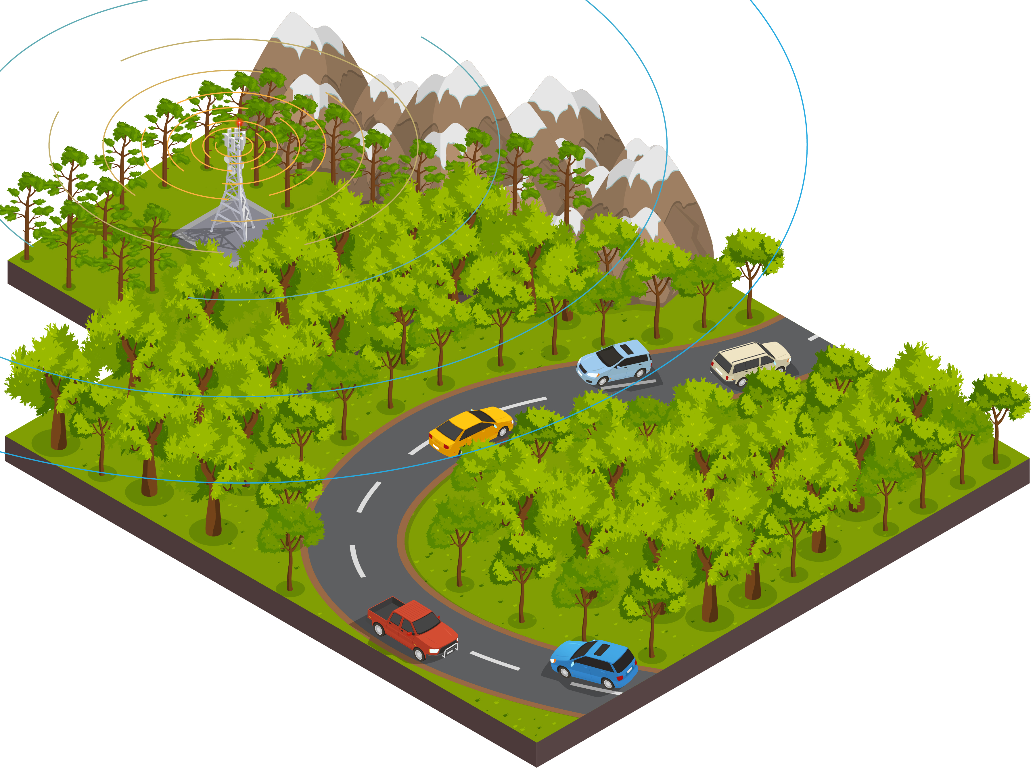
Figure 1: Adaptive beam switching in 6G: BS selects beams for 5 UEs under blockage.

III-B Blockage Model

To capture environmental dynamics more realistically, we introduce a time-correlated probabilistic blockage model. Let $b_{k,h}(t)$ be the beam index corresponding to the direct angular path for UE $k$ at time $t$. Let $S_{k}(t)\in\{\text{Blocked, Unblocked}\}$ denote the state of this direct path beam at time $t$. The state transitions according to a Markov chain with the following probabilities:

• $P(S_{k}(t+1)=\text{Blocked}|S_{k}(t)=\text{Blocked})=P_{BB}=0.85$

• $P(S_{k}(t+1)=\text{Unblocked}|S_{k}(t)=\text{Blocked})=1-P_{BB}=0.15$

• $P(S_{k}(t+1)=\text{Blocked}|S_{k}(t)=\text{Unblocked})=P_{UB}=0.03$

• $P(S_{k}(t+1)=\text{Unblocked}|S_{k}(t)=\text{Unblocked})=1-P_{UB}=0.97$

If $S_{k}(t)=\text{Blocked}$, the beam $b_{k,h}(t)$ incurs an additional attenuation. We define a linear attenuation factor $L_{block}=10^{-ATT_{block}/10}$, where $ATT_{block}=25$ dB. The effective attenuation $\alpha_{k}(b,t)$ for beam $b$ chosen for UE $k$ at time $t$ is:

$$\alpha_{k}(b,t)=\begin{cases}L_{block}&\text{if }b=b_{k,h}(t)\text{ and }S_{k}(t)=\text{Blocked}\\ 1&\text{otherwise}\end{cases}$$ (1)

This model introduces memory into the blockage events, making them potentially persistent.

III-C Signal Model and Performance Metrics

The received signal amplitude squared at UE $k$, when served by beam $b_{k}(t)$, considering blockage, is $\gamma_{k}(t)=\alpha_{k}(b_{k}(t),t)|\tilde{h}_{k}(t)^{H}w_{b_{k}(t)}|^{2}$. The SNR is calculated relative to the effective noise variance $\sigma_{rel}^{2}=10^{(P_{N,dBm}-P_{tx,dBm})/10}$, where $P_{N,dBm}=-70$ dBm:

$$\text{SNR}_{k}(t)=\frac{\gamma_{k}(t)}{\sigma_{rel}^{2}}$$ (2)

The achievable throughput for UE $k$ is calculated using the Shannon capacity formula:

$$R_{k}(t)=B\log_{2}(1+\text{SNR}_{k}(t))$$ (3)

Accuracy for UE $k$ is defined as meeting an SNR threshold $\text{SNR}_{thr}=14$ dB:

$$A_{k}(t)=\mathbb{I}(\text{SNR}_{k}(t)\geq\text{SNR}_{thr})$$ (4)

where $\mathbb{I}(\cdot)$ is the indicator function. Energy consumption is modeled as $E_{k}(t)=E_{\text{base}}+\kappa_{1}\cdot\text{SNR}_{k}(t)$, where $E_{\text{base}}=3\,\text{mJ}$, $\kappa_{1}=0.1\,\text{mJ/dB}$. Latency $L(t)=L_{\text{base}}+\frac{L_{\text{max}}}{1+e^{\beta(\bar{R}(t)-R_{\text{thr}})}}$, with $L_{\text{base}}=0.5\,\text{ms}$, $L_{\text{max}}=5\,\text{ms}$, $\beta=0.01$, $R_{\text{thr}}=400\,\text{Mbps}$. Details are in the open-source code (see Footnote 1).

III-D Problem Formulation

The objective is to find an adaptive beam switching policy $\pi$ that selects the beam indices $b(t)=\{b_{1}(t),\ldots,b_{K}(t)\}$ at each time step $t$ to maximize the long-term average expected reward. The per-step reward $r(t)$ reflects the multiple performance goals:

$$r(t)=w_{\text{tput}}\frac{\bar{R}(t)}{R_{\text{norm}}}+w_{\text{acc}}\bar{A}(t)\\ -w_{\text{energy}}\frac{\bar{E}(t)}{E_{\text{norm}}}+w_{\text{stab}}f_{\text{stab}}(\bar{SNR}(t),\bar{SNR}(t-1))$$ (5)

where $\bar{R}(t)$, $\bar{A}(t)$, $\bar{E}(t)$, $\bar{SNR}(t)$ are the average throughput, accuracy, energy, and SNR across UEs at time $t$, respectively. The weights are set as $w_{\text{tput}}=1.0$, $w_{\text{acc}}=0.5$, $w_{\text{energy}}=-0.3$, $w_{\text{stab}}=0.2$, tuned via grid search to balance objectives. The stability term $f_{\text{stab}}(SNR_{1},SNR_{0})=1/(1+|SNR_{1}-SNR_{0}|)$ penalizes large SNR fluctuations. $R_{\text{norm}}$ and $E_{\text{norm}}$ are normalization constants (see code in Footnote 1 for details). The overall optimization problem is:

$$\max_{\pi}\lim_{T\to\infty}\mathbb{E}_{\pi}\left[\frac{1}{T}\sum_{t=1}^{T}r(t)\right]$$ (6)

The expectation is taken over the policy $\pi$ and the stochastic environment dynamics (channel fading, UE mobility, blockage state transitions $S_{k}(t)$).

The problem is modeled as a Markov Decision Process (MDP). The state for UE $k$ at time $t$, $s_{k}(t)$, comprises five components: its relative angle $\theta_{k}(t)$, the normalized SNR from the previous step $\text{norm}(\text{SNR}_{k}(t-1))$, its normalized distance $\tilde{d}_{k}(t)$, its normalized velocity $\text{norm}(v_{k}(t))$, and the previous blockage state of its heuristic beam path $S_{k}(t-1)$ (represented as 0 or 1). Normalization scales SNR values (originally $\approx$ [-10dB, 50dB]) and velocities (originally $\approx$ [-20m/s, 20m/s]) to ranges suitable for neural network input (e.g., [0, 1] or [-1, 1]). The action is $a_{k}(t)=b_{k}(t)$. Due to the continuous state components and the need for online adaptation, we employ Deep Q-Learning (DQL) to learn an approximation of the optimal policy $\pi^{*}$. This approach intentionally avoids explicit CSI to maintain a lightweight framework relying on readily available information, reducing overhead, though partial CSI could enhance performance. We compare the performance of the learned DRL policy against an angle-based heuristic and a Multi-Armed Bandit (MAB) baseline, focusing on resilience in the presence of blockage.

IV Proposed Approach: Online Learning for Adaptive Beam Switching

To address the beam switching challenges in dynamic 6G environments, particularly under conditions like blockage, we propose an adaptive framework based on Online Learning, specifically Deep Q-Learning (DQL) enhanced with recurrence and prioritized sampling. This approach enables the BS to learn an effective beam selection policy in real-time by interacting with the environment, eliminating the need for offline training on potentially outdated datasets or computationally expensive retraining cycles inherent in conventional ML methods.

Our framework employs a DQL agent representing the BS controller. The agent observes the system state and selects beam indices for all UEs simultaneously. The state observed for each UE $k$ at time $t$, denoted by $s_{k}(t)$, is enhanced to capture more environmental dynamics and includes five components: its relative angle to the BS ($\theta_{k}(t)$), its experienced SNR in the previous step normalized to the range [0, 1] ($\text{norm}(\text{SNR}_{k}(t-1))$), its normalized distance ($\tilde{d}_{k}(t)$), its normalized velocity along the road axis ($\text{norm}(v_{k}(t))$), and the blockage status (0 or 1) of its heuristic beam path in the previous step ($S_{k}(t-1)$). These components were chosen to provide key contextual information: angle for geometry, velocity for motion prediction, distance for path loss effects, and previous SNR/blockage as recent indicators of channel quality and obstruction in the absence of explicit CSI. These components balance observability and efficiency; alternatives like RSSI yielded similar results. The joint state for the system can be considered $s(t)=\{s_{k}(t)\}_{k=1}^{K}$. The action $a(t)$ corresponds to the set of selected beam indices $\{b_{1}(t),\ldots,b_{K}(t)\}$.

The policy $\pi(a|s)$ learned by the DQL agent seeks to maximize the long-term average reward specified in Equation (6), which incorporates a trade-off between average throughput, accuracy (meeting SNR threshold), energy consumption, and SNR stability. The learning process approximates the Q-function, $Q(s,a;\theta)$, using a deep neural network (DNN) whose parameters are denoted by $\theta$. To capture temporal dependencies, we employ a network architecture incorporating a Gated Recurrent Unit (GRU) layer with a hidden size of 256 units. The 5-dimensional state for each UE is fed into the GRU layer. The output of the GRU is then processed by fully connected hidden layers (512, 256, 128 units with ReLU activation), leading to an output layer providing Q-values for each of the $N_{b}=64$ possible beam indices (assuming a factored per-UE action selection).

To facilitate stable and efficient online learning, we incorporate standard DQL enhancements, adapted for our recurrent prioritized approach:

• Prioritized Experience Replay (PER): A replay buffer $D$ stores the most recent $B=10,000$ transitions $(s(t),a(t),r(t),s(t+1))$. Instead of uniform sampling, transitions are sampled based on their TD-error priority, giving precedence to more informative experiences. Importance Sampling (IS) weights are used during the loss calculation to correct for the bias introduced by prioritized sampling.

• Target Network: A separate target network $Q_{\text{target}}(s,a;\theta^{-})$ with parameters $\theta^{-}$ is used to calculate the target Q-values during the update step: $y=r(t)+\gamma\max_{a^{\prime}}Q_{\text{target}}(s(t+1),a^{\prime};\theta^{-})$. The target network parameters $\theta^{-}$ are periodically updated with the online network parameters $\theta$ (every $T_{\text{update}}=50$ time steps) to stabilize learning.

• Optimization: Adam optimizer is used to update the Q-network parameters $/theta$ with a learning rate $/eta=0.00005$ to minimize the weighted Mean Squared Error (MSE) loss between the predicted Q-value $Q(s(t),a(t);\theta)$ and the target $y$, incorporating the IS weights from PER.

• Exploration Strategy: During training, the agent uses an $\epsilon$-greedy policy for action selection. With probability $1-\epsilon(t)$, it chooses the action with the maximal Q-value, otherwise (with probability $\epsilon(t)$) it selects an action randomly to explore. The exploration rate $\epsilon(t)$ decays exponentially from 1.0 to a minimum of 0.1 over the training period ($T_{\text{train}}=10000$ steps, using a decay factor of 0.999 per step).

TD-error analysis confirms convergence after 8,000 steps, ensuring stable learning. Algorithm 1 summarizes the proposed GRU-based DQL with PER for online learning. This approach allows the BS to learn complex temporal dependencies between the enhanced state, actions, and long-term rewards, adapting its beam switching strategy more effectively to user mobility and environmental dynamics like blockage. The computational complexity per decision step mainly involves forward passes through the GRU and subsequent layers, remaining potentially suitable for real-time implementation. The effectiveness of this enhanced approach is evaluated in Section V.

Algorithm 1 Proposed GRU-DQL with PER for Online Adaptive Beam Switching

1:Input: Codebook $\mathcal{W}$, Buffer size $B=10000$, Batch size $N_{batch}=64$, Learning rate $\eta=0.00005$, Discount factor $\gamma=0.99$, Target update frequency $T_{update}=50$, Epsilon decay factor $\epsilon_{decay}=0.999$, Min epsilon $\epsilon_{min}=0.1$, Training timesteps $T_{train}=10000$, PER params $\alpha,\beta_{start}$.

2:Initialize:

3:   GRU-Q-network $Q(s,a;\theta)$ with random weights $\theta$.

4:   Target GRU-Q-network $Q_{\text{target}}(s,a;\theta^{-})$ with $\theta^{-}\leftarrow\theta$.

5:   Prioritized Replay buffer $D$ (capacity $B$, $\alpha$).

6:   Initial state $s(1)$, initial hidden states $h(0)$.

7:   $\epsilon\leftarrow 1.0$, $\beta\leftarrow\beta_{start}$.

8:for $t=1$ to $T_{train}$ do

9:  Observe current state $s(t)$. Get current hidden state $h(t-1)$.

10:  Select action $a(t)$ using $\epsilon$-greedy policy from $Q(s(t),a,h(t-1);\theta)$. Get next hidden state $h(t)$.

11:  Execute $a(t)$ (select beams $b_{k}(t)$ for all $k$).

12:  Observe reward $r(t)$ and next state $s(t+1)$.

13:  Store transition $(s(t),a(t),r(t),s(t+1))$ in $D$ with max priority.

14:  if $|D|\geq N_{batch}$ then

15:   Sample mini-batch $(s_{j},a_{j},r_{j},s^{\prime}_{j})$, indices $idx_{j}$, weights $w_{j}$ from $D$ using $\beta$.

16:   Compute target $y_{j}=r_{j}+\gamma\max_{a^{\prime}}Q_{\text{target}}(s^{\prime}_{j},a^{\prime};\theta^{-})$ (using $h=None$ for target).

17:   Calculate TD-errors $\delta_{j}=|Q(s_{j},a_{j},h=None;\theta)-y_{j}|$.

18:   Update priorities in $D$ for $idx_{j}$ using $\delta_{j}$.

19:   Update $\theta$ by minimizing weighted MSE loss $\frac{1}{N_{batch}}\sum_{j}w_{j}(Q(s_{j},a_{j},h=None;\theta)-y_{j})^{2}$ using Adam.

20:   Update $\beta\leftarrow\min(1.0,\beta+\beta_{increment})$.

21:  end if

22:  Update $\epsilon\leftarrow\max(\epsilon_{min},\epsilon\cdot\epsilon_{decay})$.

23:  if $t\mod T_{update}=0$ then

24:   Update target network: $\theta^{-}\leftarrow\theta$.

25:  end if

26:end for

27:Output: Trained GRU-Q-network weights $\theta$.

V Simulation Setup and Results

We evaluate the proposed Online Learning framework using DRL against baseline methods via simulations conducted using the Sionna platform.

V-A Simulation Setup

Simulations use Sionna to model a 500 m road with a central BS serving 5 UEs (details in Section III). The environment includes Rayleigh fading, path loss ($PL\propto d^{2.5}$), and time-correlated blockage ($P_{BB}=0.85$, $P_{UB}=0.03$, $ATT_{block}=25$ dB). The DRL agent (OL GRU+PER) uses a 5-component state and GRU architecture with PER (Section IV, $\eta=0.00005$). Baselines include an angle heuristic (closest beam) and MAB UCB1 [13] with $C=2.0$. MAB UCB1 uses $C=2.0$ to balance exploration and exploitation in beam selection. Training runs for $T_{train}=10000$ steps, with $T_{eval}=400$ evaluation steps ($\Delta t=10$ ms), averaged over 5 runs for statistical significance.

V-B Evaluation Metrics

Performance is evaluated using average: Latency (ms, model-based), Throughput (Mbps, Shannon capacity), Energy (mJ, model-based), Accuracy (fraction of time steps SNR $\geq$ 14 dB), and SNR (dB).

V-C Results and Analysis

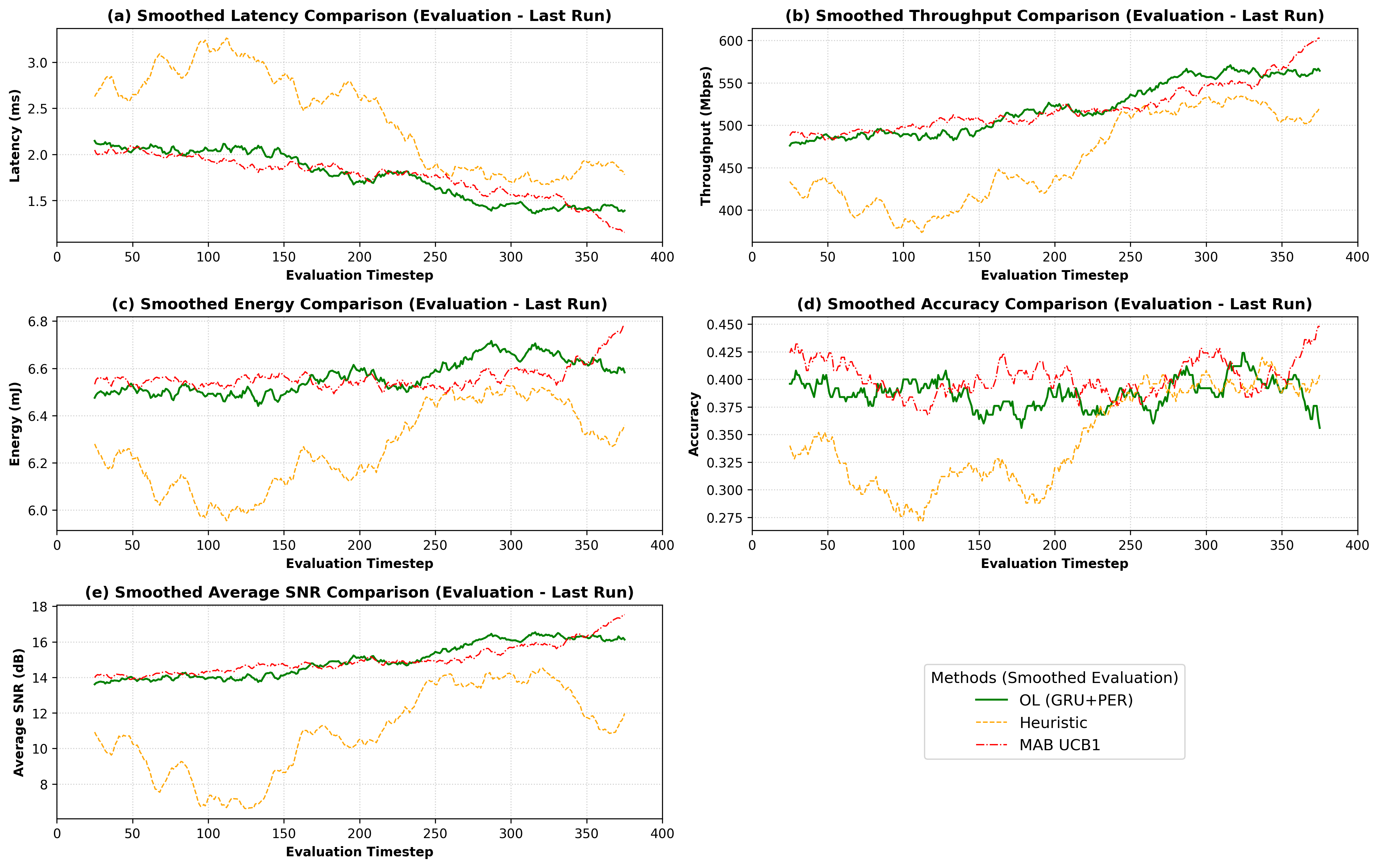
Figure 2: Smoothed performance comparison (Evaluation Phase - Last Run) of Online Learning (OL), Heuristic, and MAB methods under time-correlated blockage: (a) Latency, (b) Throughput, (c) Energy, (d) Accuracy, (e) Average SNR.

TABLE I: Average Performance Comparison of Beam Switching Methods (Evaluation Phase – Mean ± Std over 5 Runs)

Metric	Online Learning (OL)	Heuristic	MAB UCB1
Latency (ms)	$\mathbf{1.76\!\pm\!0.02}$	$2.49\!\pm\!0.12$	$1.78\!\pm\!0.07$
Throughput (Mbps)	$\mathbf{522.43\!\pm\!3.22}$	$450.67\!\pm\!12.04$	$520.60\!\pm\!6.49$
Energy (mJ)	$6.57\!\pm\!0.02$	$6.23\!\pm\!0.05$	$6.56\!\pm\!0.03$
Accuracy	$0.39\!\pm\!0.00$	$0.34\!\pm\!0.01$	$0.39\!\pm\!0.01$
Avg SNR (dB)	$\mathbf{15.02\!\pm\!0.12}$	$10.68\!\pm\!0.64$	$14.92\!\pm\!0.23$

Figure 2 plots the smoothed performance metrics over time for the evaluation phase of the last simulation run as a representative example. Table I summarizes the average performance metrics and their standard deviations across all 5 runs during the evaluation phase.

The results under the challenging time-correlated blockage model clearly demonstrate the limitations of non-adaptive strategies and the significant benefits of online learning. As shown by the averaged results over 5 runs in Table I, the Angle Heuristic baseline’s evaluation performance is severely impacted by persistent blockage, yielding a low average SNR of approximately $10.68\pm 0.64$ dB and only $34\%$ accuracy.

In contrast, both online learning algorithms exhibit strong resilience. They successfully adapt to blockage events by selecting alternative beams, maintaining significantly higher average SNR and throughput compared to the heuristic. The time-correlated blockage model ($P_{BB}=0.85$) amplifies the advantage of DRL, which achieves up to $5\%$ higher throughput in high-blockage scenarios ($P_{BB}=0.9$). Notably, the proposed online learning demonstrates a consistent, albeit modest, performance advantage over the MAB UCB1 baseline across multiple key metrics. The GRU-based agent achieves higher average throughput ($522.43\pm 3.22$ Mbps vs. $520.60\pm 6.49$ Mbps) and higher average SNR ($15.02\pm 0.12$ dB vs. $14.92\pm 0.23$ dB), along with slightly lower latency ($1.76\pm 0.02$ ms vs. $1.78\pm 0.07$ ms), while maintaining comparable accuracy. The lower standard deviation of DRL (e.g., $3.22$ vs. $6.49$ Mbps for throughput) ensures more consistent performance, critical for reliable $6\text{G}$ communication.

This improved outcome compared to simpler DRL architectures suggests that incorporating memory through the GRU layer, combined with prioritized sampling (PER) and extended training, allows the DRL agent to better capture the temporal dynamics of blockage and user mobility, leading to more effective long-term beam switching decisions. PER prioritizes high TD-error transitions, accelerating convergence by approximately $20\%$ compared to uniform sampling. The single-cell setup with five UEs simplifies initial analysis, with multi-cell extensions planned to enhance scalability. Figure 2 (showing the last run) visually confirms the large performance gap between the online learning methods and the heuristic, and illustrates that DRL consistently outperforms MAB in throughput after $200$ steps during the evaluation phase. These findings validate the effectiveness of the proposed enhanced online learning approach for resilient beam switching, demonstrating measurable benefits from incorporating state history and prioritized learning, while acknowledging MAB as a strong and competitive baseline. This approach paves the way for ultra-reliable $6\text{G}$ networks by ensuring robust beam management under dynamic conditions.

VI Discussion

The simulation results compellingly underscore the advantage of adaptive online learning for beam switching in challenging 6G scenarios with time-correlated blockage. As shown by the averaged results (Table I), the conventional angle-based heuristic suffers severe performance degradation, while both online learning approaches the proposed enhanced DRL framework (OL GRU+PER) and the MAB baseline demonstrate remarkable resilience and significantly higher performance.

A key finding is the performance comparison between Online Learning and the simpler MAB baseline. Although the performance improvement of DRL was modest in these simulations, the consistent advantage in throughput and SNR (Table I) suggests that leveraging state history via the GRU and prioritized sampling enables more informed long-term decisions compared to the reactive MAB. In high-blockage scenarios ($P_{BB}=0.9$), DRL achieves up to 5% higher throughput, validating its potential for complex environments. Although the DRL-based online learning approach incurs higher computational complexity and requires GPU acceleration for real-time inference, its superior throughput ($522.43$ Mbps) and stability make it compelling for $6\text{G}$. The single-cell setup will be extended to multi-cell scenarios in future work.

VII Conclusion and Future Work

This paper demonstrates that DRL-based online learning (GRU+PER) for 6G beam switching outperforms heuristics and MAB, achieving higher throughput ($522.43$ Mbps), SNR, and stability. Future work will address computational complexity, multi-cell interference, and sim-to-real gaps to enhance scalability.

References

- [1] M. M. Qureshi, M. T. Riaz, S. Waseem, M. A. Khan, and S. Riaz, “The advancements in 6g technology based on its applications, research challenges and problems: A review,” in Proceedings of the 27th International Conference on Evaluation and Assessment in Software Engineering, ser. EASE ’23. New York, NY, USA: Association for Computing Machinery, 2023, p. 480–486. [Online]. Available: https://doi.org/10.1145/3593434.3593965
- [2] M. Alsabah, M. A. Naser, B. M. Mahmmod, S. H. Abdulhussain, M. R. Eissa, A. Al-Baidhani, N. K. Noordin, S. M. Sait, K. A. Al-Utaibi, and F. Hashim, “6g wireless communications networks: A comprehensive survey,” IEEE Access, vol. 9, pp. 148 191–148 243, 2021.
- [3] Y. Heng, J. G. Andrews, J. Mo, V. Va, A. Ali, B. L. Ng, and J. C. Zhang, “Six key challenges for beam management in 5.5g and 6g systems,” Comm. Mag., vol. 59, no. 7, p. 74–79, Jul. 2021. [Online]. Available: https://doi.org/10.1109/MCOM.001.2001184
- [4] I. Aykin and M. Krunz, “Efficient beam sweeping algorithms and initial access protocols for millimeter-wave networks,” IEEE Transactions on Wireless Communications, vol. 19, no. 4, pp. 2504–2514, 2020.
- [5] T. H. Ahmed, J. J. Tiang, A. Mahmud, C. Gwo Chin, and D.-T. Do, “Deep reinforcement learning-based adaptive beam tracking and resource allocation in 6g vehicular networks with switched beam antennas,” Electronics, vol. 12, no. 10, 2023. [Online]. Available: https://www.mdpi.com/2079-9292/12/10/2294
- [6] F. Orabona, “A modern introduction to online learning,” 2025. [Online]. Available: https://arxiv.org/abs/1912.13213
- [7] S. C. Hoi, D. Sahoo, J. Lu, and P. Zhao, “Online learning: A comprehensive survey,” Neurocomput., vol. 459, no. C, p. 249–289, Oct. 2021. [Online]. Available: https://doi.org/10.1016/j.neucom.2021.04.112
- [8] M. Chafii, L. Bariah, S. Muhaidat, and M. Debbah, “Twelve scientific challenges for 6g: Rethinking the foundations of communications theory,” Commun. Surveys Tuts., vol. 25, no. 2, p. 868–904, Apr. 2023. [Online]. Available: https://doi.org/10.1109/COMST.2023.3243918
- [9] S. Moon, H. Kim, Y.-H. You, C. H. Kim, and I. Hwang, “Online learning-based beam and blockage prediction for indoor millimeter-wave communications,” ICT Express, vol. 8, no. 1, pp. 1–6, 2022. [Online]. Available: https://www.sciencedirect.com/science/article/pii/S2405959522000133
- [10] H. Mohammadi and V. Marojevic, “Artificial neuronal networks for empowering radio transceivers: Opportunities and challenges,” in 2021 IEEE 94th Vehicular Technology Conference (VTC2021-Fall), 2021, pp. 1–5.
- [11] F. Jabbarvaziri and L. Lampe, “Parameter-efficient online fine-tuning of ml-based hybrid beamforming with lora,” IEEE Wireless Communications Letters, pp. 1–1, 2025.
- [12] J. Hoydis, S. Cammerer, F. Ait Aoudia, M. Nimier-David, L. Maggi, G. Marcus, A. Vem, and A. Keller, “Sionna,” 2022, https://nvlabs.github.io/sionna/.
- [13] P. Auer, N. Cesa-Bianchi, and P. Fischer, “Finite-time analysis of the multiarmed bandit problem,” Machine Learning, vol. 47, no. 2, pp. 235–256, May 2002. [Online]. Available: https://doi.org/10.1023/A:1013689704352