The $k$-th Order Preserving Sets and Isoperimetric Type Inequalities for Planar Ovals

Abstract.

In this work, we introduce and investigate a new class of sets, the $k$-th Order Preserving Sets, arising naturally from the Fourier analysis of support functions associated with hedgehogs. Specifically, we focus on sets whose support functions possess a Fourier series that preserves only terms with positive indices divisible by a fixed $k$.

We explore the geometry of the $k$-th Order Middlepoint Set, defined as the set of centroids of all equiangular $k$-gons circumscribed about a given hedgehog. This set captures essential structural and symmetry-related features of the underlying geometric configuration.

We study the geometric properties of such sets and, in particular, establish an isoperimetric type inequality relating the perimeter and area of a region bounded by a simple smooth convex closed curve (an oval) $\mathcal{O}$:

$$L_{\mathcal{O}}^{2}-4\pi A_{\mathcal{O}}\geqslant 4\pi|A_{\mathcal{P}_{k}}|+2\pi|A_{\Omega_{\mathcal{O},k}}|,$$

where $L_{\mathcal{O}}$ denotes the length (perimeter) of $\mathcal{O}$, $A_{\mathcal{O}}$ is the area of the region enclosed by $\mathcal{O}$, $A_{\mathcal{P}_{k}}$ is the oriented area of the associated $k$-th Order Preserving Set $\mathcal{P}_{k}$, and $A_{\Omega_{\mathcal{O},k}}$ is the oriented area of the associated $k$-th Order Middlepoint Set $\Omega_{\mathcal{O},k}$. Moreover, we characterize the equality case: the inequality becomes an equality if and only if every equiangular circumscribed $k$-gon around $\mathcal{O}$ is a regular $k$-gon with its center of mass located at the Steiner point of $\mathcal{O}$.

1. Introduction

In recent years, the study of isoperimetric inequalities and related geometric relations has gained renewed momentum, driven by their pivotal role in understanding the behavior of geometric flows, curvature-driven evolutions, and shape optimization problems. These inequalities establish a strong link between classical geometric quantities – such as perimeter, area, and curvature – and more recently introduced concepts like the oriented areas of evolutes and Wigner caustics, with applications spanning convex and differential geometry, singularity theory, and mathematical physics – see [2, 11, 12, 13, 15, 16, 31, 34, 35, 36, 37, 39], and the literature therein.

In this work, we introduce and explore a new class of geometric sets, which we call $k$-th Order Preserving Sets. These sets arise naturally from the Fourier analysis of support functions associated with a particular class of planar objects known as hedgehogs. Specifically, we focus on support functions whose Fourier series preserve only the terms with positive indices divisible by a fixed integer $k$. This selective frequency retention reveals geometric structures that encode specific symmetry and regularity conditions. Furthermore, we introduce and study the geometry of the $k$-th Order Middlepoint Set, defined as the set of centroids of all equiangular $k$-gons circumscribed about a given hedgehog. One of the central results of our study is a new isoperimetric-type inequality (see Theorem 5.2), which connects the classical perimeter–area difference of a smooth convex closed curve $\mathcal{O}$ (an oval) with the oriented area of the associated $k$-th Order Preserving Set $\mathcal{P}_{k}$ and $k$-th Order Middlepoint Set $\Omega_{\mathcal{O},k}$:

$$L_{\mathcal{O}}^{2}-4\pi A_{\mathcal{O}}\geqslant 4\pi|A_{\mathcal{P}_{k}}|+2\pi|A_{\Omega_{\mathcal{O},k}}|,$$

where $L_{\mathcal{O}},A_{\mathcal{O}},A_{\mathcal{P}_{k}},A_{\Omega_{\mathcal{O},k}}$ are the length of $\mathcal{O}$, the area bounded by $\mathcal{O}$, the oriented area of the $k$-th Order Preserving Set $\mathcal{P}_{k}$, and the oriented area of the $k$-th Order Middlepoint Set $\Omega_{\mathcal{O},k}$, respectively. We further characterize the case of equality in this inequality: it holds with equality if and only if every equiangular circumscribed $k$-gon about $\mathcal{O}$ is a regular $k$-gon whose centroid coincides with the Steiner point of the curve $\mathcal{O}$ – a fundamental affine-invariant center introduced by Blaschke.

Interestingly, while investigating the equality case in our isoperimetric-type inequality, we found ourselves studying a problem that is, in a certain sense, dual to the classical Square Peg Problem. The Square Peg Problem – also known as Toeplitz’s conjecture – asks whether every Jordan curve contains four points that form the vertices of a square. Despite its apparent simplicity, this problem remains open in full generality and has inspired a wealth of research in topological and geometric methods (for a survey of this problem see [22]).

In contrast, our setting takes a different perspective. On the one hand, for convex curves such as ovals, the existence of a circumscribed square is a classical consequence of continuity arguments and can be established easily. On the other hand, we pose a more refined and structured question: Given that there exist infinitely many equiangular $k$-gons circumscribed about a convex curve or hedgehog, under what conditions are all of them regular and share a common centroid?

Rather than focusing on the existence of a single configuration, we study the geometry of the entire family of such polygons and the structure of the set of their centroids – a direction that leads us to the notion of the Middlepoint Set. This approach bridges harmonic analysis of support functions with classical polygonal constructions and reveals deep symmetry properties of the underlying curve.

The paper is organized as follows.

Section   2 offers a geometrical and analytical foundation for the study. It introduces the key geometric quantities associated with smooth convex curves and discusses how they can be expressed using the Fourier coefficients of the corresponding support function. This approach enables a seamless transition from classical geometric intuition to harmonic analysis, setting the groundwork for the constructions and inequalities presented in the following sections.

Section   3 develops the core concept of this work, the $k$-th Order Preserving Set, defined through the framework of isogonal points. These sets arise from families of equiangular polygonal configurations, determined by pairs of isogonal points located on a given curve. Subsequently, we analyze the Fourier-theoretic properties of these sets, viewing them as natural consequences of the geometric construction. The section also explores their structural characteristics, such as singularities, symmetry, and regularity.

Section   4 is dedicated to the introduction of the Middlepoint Set. This object is defined as the set of centroids of all equiangular $k$-gons circumscribed about a given hedgehog. It encodes important information about the symmetry and internal structure of the underlying curve and establishes a natural connection between polygonal configurations and analytic representations via support functions.

Finally, Section   5 focuses on the formulation of the main isoperimetric-type inequalities and the examination of their stability in certain special cases. We derive a lower bound for the isoperimetric deficit involving the perimeter and area of an oval, expressed in terms of the oriented areas of the corresponding $k$-th Order Preserving Set and $k$-th Order Middlepoint Set. Additionally, we analyze the equality case and investigate how geometric deviations influence a particular instance of the inequality, thereby providing insight into its stability properties.

2. Geometrical and analytical introduction

In this section, we begin by briefly presenting the essential definitions, formulas, and geometric constructions that will be used throughout the rest of the paper. These foundational elements provide the necessary context for new concepts introduced in later sections.

Let $\mathcal{H}$ denote a smooth planar curve, understood as the $C^{\infty}$-smooth map from an interval into $\mathbb{R}^{2}$. The curve $\mathcal{H}$ is said to be closed if it is a $C^{\infty}$ map from the circle $S^{1}$ to $\mathbb{R}^{2}$. It is called regular if its velocity vector never vanishes along the parameter domain. Otherwise – it is singular. A singular point is a cusp if its locally diffeomorphic (in the source and in the target) to the map $t\mapsto(t^{2},t^{3})$ at $t=0$. It is well known (e.g. see Theorem B.9.1 in [33]) that a map $f$ is a cusp at $s_{0}$ if and only if $f^{\prime}(s_{0})=0$ and $\det\big{(}f^{\prime\prime}(s_{0}),f^{\prime\prime\prime}(s_{0})\big{)}\neq 0.$ A regular, closed curve is called convex if its signed curvature maintains a constant (non-zero) sign throughout. A hedgehog is a closed planar curve that can be represented as the Minkowski difference of two convex bodies in the plane (see [19, 20]). This construction allows hedgehogs to generalize support functions beyond the convex setting. An oval, in contrast, is a simple (i.e. non-self-intersecting), smooth, regular, and closed convex curve. Ovals play a central role in classical convex geometry and serve as natural domains for the Fourier analysis of support functions. For every direction $u=(\cos s,\sin s)\in S^{1}$, the support function of an oval $\mathcal{H}$ is defined as:

$$h(s):=\sup_{x\in\mathcal{H}}\langle x,u\rangle,$$

where $\langle\cdot,\cdot\rangle$ denotes the standard Euclidean inner product. If $\mathcal{H}$ is represented as the Minkowski difference $\mathcal{H}=\mathcal{K}_{1}-\mathcal{K}_{2}$, where $\mathcal{K}_{1},\mathcal{K}_{2}$ are ovals, then the support function satisfies:

$$h(s)=h_{\mathcal{K}_{1}}(s)-h_{\mathcal{K}_{2}}(s),$$

where $h_{\mathcal{K}_{1}}$ and $h_{\mathcal{K}_{2}}$ are the classical support functions of $\mathcal{K}_{1}$ and $\mathcal{K}_{2}$, respectively.

Conversely, given a $2\pi$-periodic smooth function $h(s)$, one can obtain the parameterization of a hedgehog $\mathcal{H}$ as follows:

(2.1) $$\mathcal{H}(s) =h(s)\,u(s)+h^{\prime}(s)\,u^{\perp}(s)$$

$$=\Big{(}h(s)\cos(s)-h^{\prime}(s)\sin(s),h(s)\sin(s)+h^{\prime}(s)\cos(s)\Big{)},$$

where $u(s)=(\cos s,\sin s)$ and $u^{\perp}(s)=(-\sin s,\cos s)$ is the vector $u(s)$ rotated by $\frac{\pi}{2}$ counterclockwise.

Remark 2.1.

If $h^{\prime\prime}(s)+h(s)>0$ for all $s$, then the resulting curve $\mathcal{H}$ is convex. Otherwise, $\mathcal{H}$ may exhibit cusps or self-intersections, but still defines a valid hedgehog.

The Steiner point is a distinguished point associated with a hedgehog. It is an affine-invariant center that plays a fundamental role in convex geometry, especially in connection with support functions and affine symmetrization processes.

Definition 2.2.

Let $\mathcal{H}$ be a hedgehog. The Steiner point of $\mathcal{H}$, denoted $S(\mathcal{H})$, is defined via its support function $h(s)$ as follows:

$$S(\mathcal{H})=\frac{1}{\pi}\int_{0}^{2\pi}h(s)\,u(s)\,\mathrm{d}s,$$

where $u(s)=(\cos s,\sin s)$.

The Steiner point can be interpreted as the average of the support vectors weighted by direction.

Let $\mathcal{H}$ be a hedgehog. We define $\operatorname{rot}\left(\mathcal{H},\alpha\right)$ to be the hedgehog resulting from rotating $\mathcal{H}$ by angle $\alpha$ about its Steiner point $S(\mathcal{H})$. In particular, we denote $\mathcal{H}^{\perp}(s):=\operatorname{rot}\left(\mathcal{H},\frac{\pi}{2}\right)$. If $h(s)$ is a support function of $\mathcal{H}$, then it is obvious that $h(s-\alpha)$ is a support function of $\operatorname{rot}\left(\mathcal{H},\alpha\right)$. In particular:

(2.2) $$\mathcal{H}^{\perp}(s)=-\Big{(}h(s)\sin(s)+h^{\prime}(s)\cos(s),-h(s)\cos(s)+h^{\prime}(s)\sin(s)\Big{)}.$$

Next, we introduce a natural generalization of the concept of area of a region to the oriented area of a closed curve.

Definition 2.3.

Let $\mathcal{O}$ be an oriented, piecewise-smooth closed curve. Then the oriented area of $\mathcal{O}$ is

$$A_{\mathcal{O}}:=\frac{1}{2}\int_{\mathcal{O}}-y\mathrm{d}x+x\mathrm{d}y=\iint_{\mathbb{R}^{2}}w_{C}(x,y)\mathrm{d}x\mathrm{d}y,$$

where $w_{C}(x,y)$ is the winding number of $C$ around a point $(x,y)\in\mathbb{R}^{2}$.

Now, since the support function $h$ is smooth and $2\pi$-periodic, we express it via its Fourier series expansion as follows:

$$h(s)=a_{0}+\sum_{n=1}^{\infty}\left(a_{n}\cos ns+b_{n}\sin ns\right).$$

One can check that the area (Cauchy’s formula), length of the oval (Blaschke’s formula) $\mathcal{O}$, and the Steiner point of $\mathcal{O}$ are described by the following formulae in terms of the coefficients of the Fourier series of it’s Minkowski support function $h$:

(2.3) $$A_{\mathcal{O}} =\frac{1}{2}\int_{0}^{2\pi}\Big{(}h^{2}(s)-h^{\prime 2}(s)\Big{)}\mathrm{d}s=\pi a_{0}-\frac{\pi}{2}\sum_{\begin{subarray}{c}n=2\end{subarray}}^{\infty}(n^{2}-1)(a_{n}^{2}+b_{n}^{2}),$$

(2.4) $$L_{\mathcal{O}} =\int_{0}^{2\pi}h(s)\mathrm{d}s=2\pi a_{0},$$

(2.5) $$S(\mathcal{O}) =(a_{1},b_{1}).$$

We call the quantity

(2.6) $$L^{2}_{\mathcal{O}}-4\pi A_{\mathcal{O}}=2\pi^{2}\sum_{n=2}^{\infty}(n^{2}-1)(a_{n}^{2}+b_{n}^{2})$$

the isoperimetric deficit. Furthermore, in the case of a hedgehog $\mathcal{H}$, one gets the formula for it’s oriented area:

(2.7) $$A_{\mathcal{H}} =\frac{1}{2}\int_{0}^{2\pi}\Big{(}h^{2}(s)-h^{\prime 2}(s)\Big{)}\mathrm{d}s=\pi a_{0}-\frac{\pi}{2}\sum_{\begin{subarray}{c}n=2\end{subarray}}^{\infty}(n^{2}-1)(a_{n}^{2}+b_{n}^{2}).$$

In recent years, the study of hedgehogs has gained considerable attention within the field of convex, differential geometry, and singularity theory. This renewed interest is reflected in the emergence of new isoperimetric-type inequalities and properties, not only in the classical Euclidean setting, but also in more general geometric contexts, including affine, spherical, and hyperbolic spaces (see, for instance, [21, 23, 24, 25, 26, 28, 32, 36, 39], and the literature therein).

Furthermore, hedgehog-related constructions have appeared in the formulation and refinement of generalized versions of the Gauss–Bonnet theorem, where curvature and topological invariants are analyzed through the lens of support functions and their harmonic structure. These developments underscore the growing role of hedgehogs as a unifying concept bridging classical geometry, Fourier analysis, and global geometric invariants (see [10, 38]).

3. The k-th Order Preserving Set

In this section, we introduce and study a new class of geometric objects that emerge naturally from the Fourier analysis of support functions – the $k$-th Order Preserving Sets. These sets arise when one imposes a specific harmonic constraint on the support function of a hedgehog: namely, that only the positive-frequency Fourier components whose indices are divisible by a fixed integer $k$ are retained.

This seemingly simple restriction leads to rich geometric behavior and surprising structural properties. The resulting sets generalize classical notions of symmetry, regularity, and curvature, while also offering a new perspective on the relationship between analytic representations (via the Fourier series) and geometric shape.

From a broader perspective, this construction can be seen as a type of Fourier projection onto a $k$-harmonic subspace, which preserves only selected symmetries and periodicities of the original curve. This idea resonates with classical problems in geometric tomography, spectral geometry, and affine differential geometry.

Definition 3.1.

Let $\mathcal{H}$ be a positively oriented hedgehog and $k>2$ be an integer. We call the points $a_{1},\ldots,a_{k}\in\mathcal{H}$ an isogonal family of points if the tangent lines to $\mathcal{H}$ at points $a_{i},a_{i+1}$ intersect at a certain angle, constant for every such pair of points $a_{i},a_{i+1}$ (assuming $a_{k+1}=a_{1}$). Let $\mathcal{H}^{\perp}$ be the hedgehog $\mathcal{H}$ rotated counter-clockwise $90^{\circ}$ about the Steiner point of $\mathcal{H}$. Let’s consider the parameterization of $\mathcal{H}$ as described by the equation (2.1). We shall also consider the parameterization of $\mathcal{H}^{\perp}$ derived from the parameterization of $\mathcal{H}$ as in the equation (2.2). Let $a=\mathcal{H}(s)$, for a given $s\in[0,2\pi]$, we uniquely characterize $a^{\perp}=\mathcal{H}^{\perp}(s)$. We shall denote the points $a_{1}^{\perp},\ldots,a_{k}^{\perp}\in\mathcal{H}^{\perp}$ which constitute an isogonal family of points in $\mathcal{H}^{\perp}$, such that for every $i$ the tangent line to $\mathcal{H}^{\perp}$ at $a_{i}^{\perp}$ is perpendicular to the tangent line to $\mathcal{H}$ at $a_{i}$.

Example 3.2.

We will consider an oval $\mathcal{O}$ with a support function $h(s)=20+\sin(2s)+\cos(3s)$ and $k=3$ (see Figure 1).

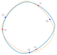
Figure 1. An oval $\mathcal{O}$ (solid) with $a_{1},a_{2},a_{3}$ an isogonal family of points (red) and $\mathcal{O}^{\perp}$ (dashed) with $a_{1}^{\perp},a_{2}^{\perp},a_{3}^{\perp}$ (blue)

Definition 3.3.

For a given $k>2$, we shall define the $k$-th Order Preserving Set as:

$$\mathcal{P}_{k}:=\Bigg{\{}\frac{1}{k}\sum_{j=1}^{k}\Bigg{(}\cos\left(\frac{2\pi j}{k}\right)\cdot a_{j}-\sin\left(\frac{2\pi j}{k}\right)\cdot a_{j}^{\perp}\Bigg{)}+\overline{w}\cdot\mathbbm{n}(a_{1})\colon$$

$$\{a_{j}\}_{j=1}^{j=k}\text{ is an isogonal family of points of $\mathcal{H}$ }\Bigg{\}}.$$

where $\overline{w}$ is the average width of $\mathcal{H}$ and $\mathbbm{n}(a)$ is a continuous unit normal vector field to $\mathcal{H}$ at the point $a$, compatible with the orientation of $\mathcal{H}$. We treat $\mathcal{P}_{k}$ as a subset of a vector space $\mathbb{R}^{2}$.

Remark 3.4.

In this paper, we focus on the case $k>2$. When $k=2$, the corresponding ”isogonal family” can be treated as pairs of distinct points $a_{1},a_{2}\in\mathcal{H}$ such that the tangent lines to $\mathcal{H}$ at those points are parallel (such pair of points is usually called a parallel pair). In this setting, the associated $2$-nd Order Preserving Set reduces to a known object called the Constant Width Measure Set, which has been studied in [28, 37, 39].

Example 3.5.

Let’s consider an oval $\mathcal{O}$ with a support function $h(s)=30+\sin(2s)+\cos(3s)+\cos(4s)$ and it’s $3$-rd and $4$-th Order Preserving Sets (see Figure 2). Note that the number of cusps in these examples are divisible by $k$ as it should be (see Proposition  3.13).

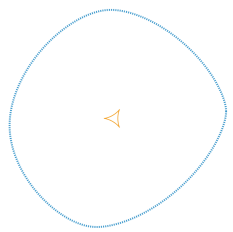
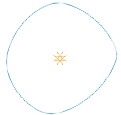
Figure 2. An oval $\mathcal{O}$ and (i) $\mathcal{P}_{3}$, (ii) $\mathcal{P}_{4}$

Example 3.6.

Let’s consider a singular hedgehog $\mathcal{H}$ with a support function $h(s)=10+\sin(2s)+\cos(3s)+\cos(6s)$ and it’s $3$-rd Order Preserving Sets (see Figure 3).

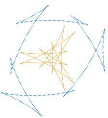
Figure 3. A hedgehog $\mathcal{H}$ and $\mathcal{P}_{3}$

Proposition 3.7.

Let $\mathcal{H}$ be a hedgehog with the support function $h:[0,2\pi]\to\mathbb{R}$, where $h(s)=a_{0}+\sum_{n=1}^{\infty}a_{n}\cos(ns)+b_{n}\sin(ns)$ is its Fourier series representation, and let the average width of $\mathcal{H}$ be $\overline{w}$. Then, the support function of its $k$-th Order Preserving Set $\mathcal{P}_{k}$ is given by the formula:

$$h_{k}(s)=\frac{1}{k}\sum_{j=0}^{k-1}h\left(s+\frac{2\pi j}{k}\right)-\overline{w},$$

and its Fourier series representation is as follows:

(3.1) $$h_{k}(s)=\sum_{k\mid n,\ n>1}^{\infty}a_{n}\cos(ns)+b_{n}\sin(ns).$$

Proof.

One may observe that the points $\mathcal{H}(s),\ldots,\mathcal{H}\left(s+\frac{2\pi(k-1)}{k}\right)$, for a given $s\in[0,2\pi]$, constitute an isogonal family of $\mathcal{H}$. Then, the parameterization of the $k$-th Order Preserving Set is:

$$\mathcal{P}_{k}(s)=\frac{1}{k}\sum_{j=1}^{k}\Bigg{(}\cos\left(\frac{2\pi j}{k}\right)\cdot\mathcal{H}\left(s+\frac{2\pi j}{k}\right)-\sin\left(\frac{2\pi j}{k}\right)\cdot\mathcal{H}^{\perp}\left(s+\frac{2\pi j}{k}\right)\Bigg{)}+\overline{w}\cdot\mathbbm{n}(s).$$

Naturally, the point $\mathcal{H}^{\perp}(s+\frac{2\pi j}{k})$ is understood as in Definition 3.1. Using the parameterization (2.2) of $\mathcal{H}^{\perp}$ we obtain the following equalities:

$$\mathcal{P}_{k} (s)=\frac{1}{k}\sum_{j=1}^{k}\Bigg{(}\cos\Big{(}\frac{2\pi j}{k}\Big{)}\cdot\Bigg{(}h\Big{(}s+\frac{2\pi j}{k}\Big{)}\cos\Big{(}s+\frac{2\pi j}{k}\Big{)}-h^{\prime}\Big{(}s+\frac{2\pi j}{k}\Big{)}\sin\Big{(}s+\frac{2\pi j}{k}\Big{)},$$

$$h\Big{(}s+\frac{2\pi j}{k}\Big{)}\sin\Big{(}s+\frac{2\pi j}{k}\Big{)}+h^{\prime}\Big{(}s+\frac{2\pi j}{k}\Big{)}\cos\Big{(}s+\frac{2\pi j}{k}\Big{)}\Bigg{)}+$$

$$+\frac{1}{k}\sum_{j=1}^{k}\Bigg{(}\sin\Big{(}\frac{2\pi j}{k}\Big{)}\cdot\Bigg{(}h\Big{(}s+\frac{2\pi j}{k}\Big{)}\sin\Big{(}s+\frac{2\pi j}{k}\Big{)}+h^{\prime}\Big{(}s+\frac{2\pi j}{k}\Big{)}\cos\Big{(}s+\frac{2\pi j}{k}\Big{)},$$

$$-h\Big{(}s+\frac{2\pi j}{k}\Big{)}\cos\Big{(}s+\frac{2\pi j}{k}\Big{)}+h^{\prime}\Big{(}s+\frac{2\pi j}{k}\Big{)}\sin\Big{(}s+\frac{2\pi j}{k}\Big{)}\Bigg{)}\Bigg{)}-\overline{w}\cdot\big{(}\cos(s),\sin(s)\big{)}$$

$$=\frac{1}{k}\sum_{j=1}^{k}\Bigg{(}\Big{(}h(s+\frac{2\pi j}{k})\cos(s)-h^{\prime}(s+\frac{2\pi j}{k})\sin(s),$$

$$h\Big{(}s+\frac{2\pi j}{k}\Big{)}\sin(s)+h^{\prime}\Big{(}s+\frac{2\pi j}{k}\Big{)}\cos(s)\Bigg{)}-\overline{w}\cdot\big{(}\cos(s),\sin(s)\big{)}$$

$$=\Big{(}\cos(s),\sin(s)\Big{)}\cdot\Bigg{(}\frac{1}{k}\sum_{j=1}^{k}h\Big{(}s+\frac{2\pi j}{k}\Big{)}-\overline{w}\Bigg{)}+\Big{(}-\sin(s),\cos(s)\Big{)}\cdot\Bigg{(}\frac{1}{k}\sum_{j=1}^{k}h^{\prime}\Big{(}s+\frac{2\pi j}{k}\Big{)}\Bigg{)}.$$

Now, setting $h_{k}(s)=\frac{1}{k}\sum_{j=0}^{k-1}h\left(s+\frac{2\pi j}{k}\right)-\overline{w}$, we obtain $P_{k}(s)$ in the form of equation (2.1). Therefore, we end the first part of the proof. To derive equation (3.1), one can simplify the aforementioned form of $h_{k}$ by leveraging the properties of Fourier and geometric series. ∎

Remark 3.8.

One may notice that as $k$ tends to infinity, the Fourier coefficients of $h_{k}$ disappear. Hence, the limit $\mathcal{P}_{\infty}$ is a point (the point of origin).

Remark 3.9.

Let’s consider the Fourier expansion of the support function $h(s)=a_{0}+\sum_{n=1}^{\infty}a_{n}\cos(ns)+b_{n}\sin(ns),\;s\in[0,2\pi]$. By Proposition 3.7 the support function of the $k$-th Order Preserving Set $h_{k}$ only preserves the Fourier indices divisible by $k$, with the exception of $0$. Thus, by the equation (3.1) one gets that:

$$h_{k}^{\prime}(s)=\sum_{k\mid n,\;n>1}^{\infty}n\Big{(}b_{n}\cos(ns)-a_{n}\sin(ns)\Big{)}$$

and

$$h_{k}^{\prime\prime}(s)=-\sum_{k\mid n,\;n>1}^{\infty}n^{2}\Big{(}a_{n}\cos(ns)+b_{n}\sin(ns)\Big{)}.$$

Remark 3.10.

Let $\mathcal{H}$ be a hedgehog. By analysis of Fourier series it is evident, that $\mathcal{P}_{k}$ is a point if and only if the support function of $\mathcal{H}$ is of the form: $h(s)=a_{0}+\sum_{k\nmid n}a_{n}\cos(ns)+b_{n}\sin(ns)$. By Definition 3.3, the set $\mathcal{P}_{k}$ is a point if and only if $\frac{1}{k}\sum_{j=1}^{k}\left(\sin\left(\frac{2\pi j}{k}\right)\cdot a_{j}^{\perp}-\cos\left(\frac{2\pi j}{k}\right)\cdot a_{j}\right)=\overline{w}_{{M}}\cdot\mathbbm{n}(a_{1})$ for all isogonal families of points $a_{1},\ldots,a_{k}$, which means that the length of the vector $\sum_{j=1}^{k}\left(\sin\left(\frac{2\pi j}{k}\right)\cdot a_{j}^{\perp}-\cos\left(\frac{2\pi j}{k}\right)\cdot a_{j}\right)$ is always constant and equal to $k\overline{w}$.

Remark 3.11.

By Proposition 3.7, we may parametrize the $k$-th Order Preserving Set as follows:

$$\mathcal{P}_{k}(s)=\Big{(}h_{k}(s)\cos(s)-h_{k}^{\prime}(s)\sin(s),h_{k}(s)\sin(s)+h_{k}^{\prime}(s)\cos(s)\Big{)},\ s\in[0,2\pi].$$

Proposition 3.12.

Let’s consider a hedgehog $\mathcal{H}$, it’s $k$-th Order Preserving Set $\mathcal{P}_{k}$, and their respective parameterizations. Then, the tangent line to $\mathcal{H}$ at $\mathcal{H}(s)$ (for some $s\in[0,2\pi]$) is parallel to the tangent line to $\mathcal{P}_{k}$ at the point $\mathcal{P}_{k}(s)$, provided it is non-singular.

Proof.

Differentiating the parameterizations at some $s\in[0,2\pi]$, where $\mathcal{P}_{k}(s)$ is non-singular, immediately yields the desired result:

$$\mathcal{H}^{\prime}(s) =\Big{(}h(s)+h^{\prime\prime}(s)\Big{)}\cdot\Big{(}-\sin(s),\cos(s)\Big{)},$$

$$\mathcal{P}^{\prime}_{k}(s) =\Big{(}h_{k}(s)+h^{\prime\prime}_{k}(s)\Big{)}\cdot\Big{(}-\sin(s),\cos(s)\Big{)}.$$

∎

We illustrate Proposition 3.12 in Figure  4.

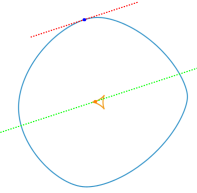
Figure 4. Consider an oval $\mathcal{O}$ with a support function $h(s)=30+\sin(2s)+\cos(3s)+\cos(4s)$. The tangent line to the $\mathcal{O}$ at $\mathcal{O}(\frac{3\pi}{5})$ is parallel to the tangent line to $\mathcal{P}_{3}$ at $\mathcal{P}_{3}\left(\frac{3\pi}{5}\right)$

Proposition 3.13.

Let $\mathcal{H}$ be a hedgehog. Then, for $k>2$, if there are finitely many singularities, the number of singularities of the $k$-th Order Preserving Set $\mathcal{P}_{k}$ is positive and divisible by $k$.

Proof.

Let’s consider our hedgehog’s support function $h:[0,2\pi]\to\mathbb{R}$ and it’s mean width $\overline{w}$. Differentiating the parameterization of $\mathcal{P}_{k}(s)$ one gets that:

$$\mathcal{P}_{k}^{\prime}(s)=\Big{(}h_{k}(s)+h_{k}^{\prime\prime}(s)\Big{)}\cdot\Big{(}-\sin(s),\cos(s)\Big{)}.$$

Should there exist such $s_{0}\in[0,2\pi]$ that $\mathcal{P}_{k}^{\prime}(s_{0})=0$, singularities will also appear at points $s_{0}+\frac{2\pi}{k},\ldots,s_{0}+\frac{2\pi(k-1)}{k}$. Indeed, taking Remark 3.9 into account, we obtain that:

$$0=h_{k}(s_{0})+h_{k}^{\prime\prime}(s_{0})=\sum_{k\mid n,\;n>1}^{\infty}\Big{(}1-n^{2}\Big{)}\cdot\Big{(}a_{n}\cos(ns_{0})+b_{n}\sin(ns_{0})\Big{)}.$$

For any $j\in\{1,\ldots,k-1\}$ we may observe that:

$$h_{k}\Big{(}s_{0}+\frac{2\pi j}{k}\Big{)}+h_{k}^{\prime\prime}\Big{(}s_{0}+\frac{2\pi j}{k}\Big{)}$$

$$=\sum_{k\mid n,\;n>1}^{\infty}\Big{(}1-n^{2}\Big{)}\cdot\Bigg{(}a_{n}\cos\Big{(}ns_{0}+n\frac{2\pi j}{k}\Big{)}+b_{n}\sin\Big{(}ns_{0}+n\frac{2\pi j}{k}\Big{)}\Bigg{)}$$

$$=\sum_{k\mid n,\;n>1}^{\infty}\Big{(}1-n^{2}\Big{)}\cdot\Big{(}a_{n}\cos(ns_{0})+b_{n}\sin(ns_{0})\Big{)}$$

$$=h_{k}(s_{0})+h_{k}^{\prime\prime}(s_{0})=0.$$

Furthermore, we know that such a point $s_{0}$ must exist, since the $0$-th coefficient of $h_{k}$’s Fourier expansion is $0$. Moreover, since there are finitely many singularities, all of them are isolated. ∎

Theorem 3.14.

Let $\mathcal{H}$ be a positively oriented hedgehog. Let $\rho_{\mathcal{H}}(a)$ denote the radius of curvature of $\mathcal{H}$ at $a$. Let $a_{1},\ldots,a_{k}$ be an isogonal family of points in $\mathcal{H}$ and let $q=\frac{1}{k}\sum_{j=1}^{k}\Bigg{(}\cos\left(\frac{2\pi j}{k}\right)\cdot a_{j}-\sin\left(\frac{2\pi j}{k}\right)\cdot a_{j}^{\perp}\Bigg{)}+\overline{w}\cdot\mathbbm{n}(a_{1})$ be a non-singular point of $\mathcal{P}_{k}$. Then the signed radius of curvature of $\mathcal{P}_{k}$ at $q$ is equal

(3.2) $$\rho_{\mathcal{P}_{k}}(q)=\frac{1}{k}\sum_{j=1}^{k}\rho_{\mathcal{H}}\left(a_{j}\right)-\overline{w}.$$

Whereas $\rho_{\mathcal{H}}(a_{1}),\ldots\rho_{\mathcal{H}}(a_{k})$ denote the signed radii of curvature of $\mathcal{H}$ at $a_{1},\ldots,a_{k}$, respectively.

Proof.

Let us consider the parameterization of $\mathcal{H}$, then $a_{j}=\mathcal{H}\Big{(}s+\frac{2\pi j}{k}\Big{)}$. It is known that the signed radius of curvature of a hedgehog with a support function $h$ is given by the following formula: $\rho(s)=h(s)+h^{\prime\prime}(s)$. Therefore, one may notice that:

$$\rho_{\mathcal{P}_{k}}(s) =h_{k}(s)+h_{k}^{\prime\prime}(s)=\frac{1}{k}\sum_{j=1}^{k}h\Big{(}s+\frac{2\pi j}{k}\Big{)}-\overline{w}+\frac{1}{k}\sum_{j=1}^{k}h^{\prime\prime}\Big{(}s+\frac{2\pi j}{k}\Big{)}$$

$$=\frac{1}{k}\sum_{j=1}^{k}\rho_{\mathcal{H}}\Big{(}s+\frac{2\pi j}{k}\Big{)}-\overline{w}.$$

∎

Leveraging the property that a hedgehog $\mathcal{H}$ is singular at points where its radius of curvature vanishes, and noting that a singularity at $\mathcal{H}(s)$, for $s\in[0,2\pi]$, is a cusp if and only if $\det\left(\mathcal{H}^{\prime\prime}(s),\mathcal{H}^{\prime\prime\prime}(s)\right)\neq 0$, we can derive through direct calculation the following proposition:

Proposition 3.15.

Let $\mathcal{H}$ be a positively oriented hedgehog of an average width equal to $\overline{w}$. Let $\mathbbm{n}$ be a continuous unit normal vector field to $\mathcal{H}$. Let $a_{1},\ldots,a_{k}$ be an isogonal family of points in $\mathcal{H}$. Let $\rho_{\mathcal{H}}(a_{1}),\ldots\rho_{\mathcal{H}}(a_{k})$ denote the signed radii of curvature of $\mathcal{H}$ at $a_{1},\ldots,a_{k}$, respectively. The $k$-th Order Preserving Set is singular at the point $\frac{1}{k}\sum_{j=1}^{k}\left(\cos\left(\frac{2\pi j}{k}\right)\cdot a_{j}-\sin\left(\frac{2\pi j}{k}\right)\cdot a_{j}^{\perp}\right)+\overline{w}\cdot\mathbbm{n}(a_{1})$ if and only if the mean signed radius of curvature at the points $a_{1},\ldots,a_{k}$ is equal to the average width $\overline{w}$ i.e.

(3.3) $$\frac{1}{k}\sum_{j=1}^{k}\rho_{\mathcal{H}}\left(a_{j}\right)=\overline{w}.$$

Furthermore, considering the differentiated parameterizations of the $k$-th Order Preserving Set, the singular point $\mathcal{P}_{k}(s)$ is a cusp if and only if $\sum_{j=1}^{k}\rho^{\prime}_{\mathcal{H}}\Big{(}s+\frac{2\pi j}{k}\Big{)}\neq 0$.

4. The Middlepoint Set

In this section, let us start with a simple observation considering the behavior of periodic functions:

Proposition 4.1.

Let us consider a $2\pi$-periodic, smooth function $f$ and a natural number $k$. The function $f$ is $\frac{2\pi}{k}$-periodic if and only if

$$\forall_{x\in[0,2\pi]}\ f(x)=a_{0}+\sum_{k\mid n,\;n>1}a_{n}\cos(nx)+b_{n}\sin(nx).$$

Let us consider a hedgehog $\mathcal{H}$, it’s Minkowski support function $h$ and some integer $k>2$. Considering the Fourier expansion of $h$, that is,

$$h(s)=a_{0}+\sum_{n=1}^{\infty}a_{n}\cos(ns)+b_{n}\sin(ns).$$

The Steiner point of $\mathcal{H}$ is $(a_{1},b_{1})$ – see (2.5). Since the coefficients $a_{1}\cos(s),\ b_{1}\sin(s)$ account only for translation of the hedgehog, we will translate the whole system so that the Steiner point of $\mathcal{H}$ is in $(0,0)$. Let us consider any $s\in[0,2\pi]$. The support function generates an equiangular $k$-gon with the distances from the origin to its sides given by $h(s),h\left(s+\frac{2\pi}{k}\right),\ldots,h\left(s+\frac{2\pi(k-1)}{k}\right)$. These sides are contained in tangent lines to $\mathcal{H}$ at $\mathcal{H}(s),\ldots,\mathcal{H}\left(s+\frac{2\pi(k-1)}{k}\right)$, respectively. A straightforward geometric observation reveals that our support function is $\frac{2\pi}{k}$-periodic if and only if every equiangular $k$-gon circumscribed about $\mathcal{H}$ is a regular $k$-gon with it’s center of mass in $(0,0)$. By Proposition  4.1 we have that $\frac{2\pi}{k}$-periodicity is equivalent to the support function retaining only indices divisible by $k$ (including the index $0$ sic!). Returning with our translation, we obtain the following result:

Proposition 4.2.

Every equiangular $k$-gon circumscribed about $\mathcal{H}$ is a regular $k$-gon with its center of mass in the Steiner point of $\mathcal{H}$ if and only if the Fourier expansion of the support function retains only indices divisible by $k$ and its first harmonics, i.e.

$$h(s)=a_{0}+a_{1}\cos(s)+b_{1}\sin(s)+\sum_{k\mid n}a_{n}\cos(ns)+b_{n}\sin(ns).$$

This proposition is illustrated in Figure   5.

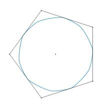
Figure 5. A hedgehog $\mathcal{H}$ with a support function $h(s)=130+\sin(5s)+\sin(10s)$, a regular circumscribed pentagon, and the singleton $\Omega_{\mathcal{H},5}$

Remark 4.3.

In analogy with Remark 3.4, the case $k=2$ corresponds to ”isogonal pairs” that can be interpreted as parallel pairs of points on the curve $\mathcal{H}$. The set of midpoints of all such parallel pairs is known in the literature by many names – as the Wigner caustic, the middle hedgehogs, defect of symmetry – and has many applications, including the isoperimetric-type problems (see [1, 3, 4, 5, 6, 7, 8, 9, 10, 14, 17, 29, 30, 36], and the references therein). It is worth noting that, although the Wigner caustic is typically a highly singular set, the Middlepoint Set exhibits a different behavior: in most cases, it is smooth and free of singularities.

Definition 4.4.

Let $\mathcal{H}$ be a hedgehog and $k$ a natural number. Let us consider the family of equiangular $k$-gons circumscribed about $\mathcal{H}$. We will call the family of the centers of mass of such $k$-gons the $k$-th Order Middlepoint Set $\Omega_{\mathcal{H},k}$.

Example 4.5.

Let’s consider a hedgehog $\mathcal{H}$ with a support function $h(s)=10+\sin(2s)+\cos(3s)+\cos(4s)+\cos(5s)$ and it’s $3$-rd Order Middlepoint Set (see Figure 6).

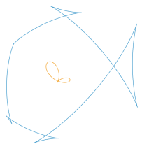
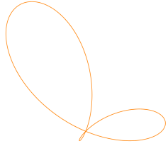
Figure 6. (i) The hedgehog $\mathcal{H}$ and $\Omega_{\mathcal{H},3}$, (ii) $\Omega_{\mathcal{H},3}$

Building on the geometric construction of equiangular $k$-gons described earlier, a straightforward analytical proof demonstrates that the $k$-th Order Midpoint Set can be elegantly parametrized:

(4.1) $$\Omega_{\mathcal{H},k}(s)=\frac{2}{k}\sum_{j=1}^{k}h\Big{(}s+\frac{2\pi j}{k}\Big{)}\Bigg{(}\cos\Big{(}s+\frac{2\pi j}{k}\Big{)},\sin\Big{(}s+\frac{2\pi j}{k}\Big{)}\Bigg{)}.$$

Allowing the parameter $s$ to vary over the interval $[0,2\pi]$ in the parameterization (4.1) yields a $k$-fold covering of the $k$-th Order Middlepoint Set. Hence, it suffices to consider the restricted interval $s\in\left[0,\tfrac{2\pi}{k}\right]$ to describe the entire set without redundancy.

From these considerations, by direct calculations, one easily deduces the following proposition.

Proposition 4.6.

The $k$-th Order Middlepoint Set $\Omega_{\mathcal{H},k}$ of a given hedgehog $\mathcal{H}$ is a point if and only if the support function of $\mathcal{H}$ is of the following form:

(4.2) $$h(s)=\sum_{k\nmid n+1\ \land\ k\nmid n-1,}a_{n}\cos(ns)+b_{n}\sin(ns).$$

Remark 4.7.

A rotor in a regular polygon is a convex closed curve that remains in continuous contact with the sides of the polygon while being fully rotated within it. In other words, it can be rotated through a full angle inside the polygon without losing contact with its boundary.

Meissner ([18]) demonstrated that such rotors in an $k$-sided regular polygon can be described analytically using their support functions:

$$h(s)=a_{0}+\sum_{k\mid n+1\ \vee\ k\mid n-1,}a_{n}\cos(ns)+b_{n}\sin(ns).$$

In other words, by Proposition 4.6, the degeneration of the Middlepoint Set to a single point is equivalent to $\mathcal{H}$ behaving, in a certain geometric sense, like the inverse harmonic counterpart of a rotor. A recent work (see [27]) investigates a dual problem to that of rotors: it characterizes curves along which a regular polygon can rotate while keeping all its vertices on the curve throughout the motion.

Note that the support function of the hedgehog in Figure 5 is of the form (4.2) – therefore the corresponding $k$-th Order Middlepoint Set is a point. The opposite situation occurs with the hedgehog in Figure 6.

To conclude this section, we establish a lemma giving an explicit expression for the oriented area of the $k$-th Order Middlepoint Set, which will serve as a crucial ingredient in the reasoning in the proof of the isoperimetric inequality in the next section.

Lemma 4.8.

Let $k\in\mathbb{N}$, $k>2$, $\mathcal{H}$ be a hedgehog, and let

$$h(s)=a_{0}+\sum_{n=1}^{\infty}a_{n}\cos(ns)+b_{n}\sin(ns)$$

be the support function of $\mathcal{H}$. Then the oriented area of the $k$-th Order MiddlePoint Set is given by the following formula:

(4.3) $$A_{\Omega_{\mathcal{H},k}}=\pi\sum_{n=1}^{\infty}n(a^{2}_{kn-1}+b^{2}_{kn-1}-a^{2}_{kn+1}-b^{2}_{kn+1}).$$

Proof.

Considering the parameterization given by the equation   (4.1) and applying Green’s theorem, one can get the following expression (in terms of Fourier coefficients of the expansion of $h$ – the Minkowski support function of $\mathcal{H}$) for the oriented area of the $k$-th Order Middlepoint Set is in the form (4.3). ∎

By Lemma 4.8, the Middlepoint Set may have positive, negative, or even zero oriented area, as illustrated in Figure 7 in the cases of $4$-th Order Middlepoint Sets. The support functions of the ovals corresponding to the Middlepoint Sets in Figure 7 are as follows:

• $h(s)=81+\sin(3s)-\sin(5s)+\sin(7s)$ for Figure 7(a),

• $h(s)=105+\sin(3s)-2\sin(5s)+\sin(7s)$ for Figure 7(b),

• $h(s)=108+\sqrt{2}\sin(3s)-2\sin(5s)+\sin(7s)$ for Figure 7(c).

It is also worth noting that this set is not necessarily a hedgehog.

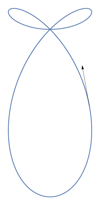
(a) Positive

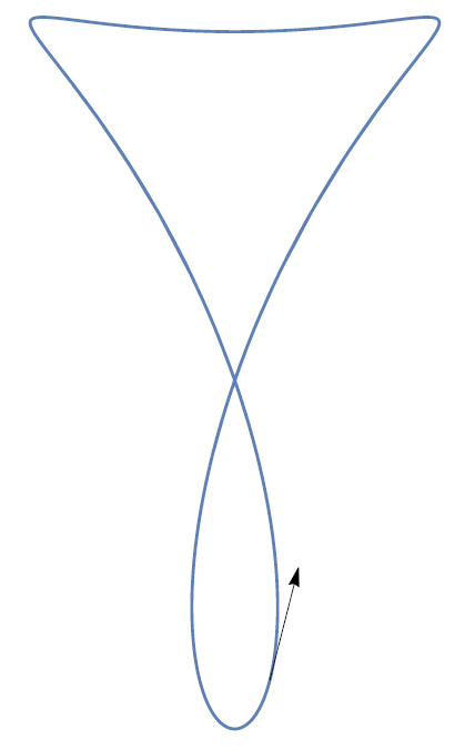
(b) Negative

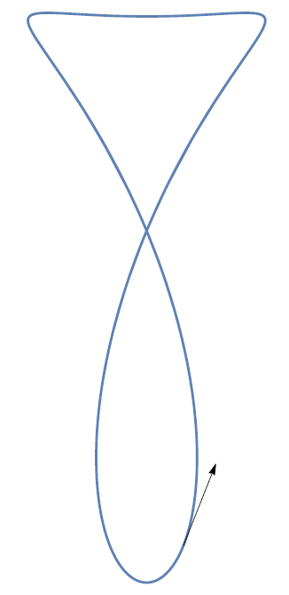
(c) Zero

Figure 7. Middlepoint Sets with varying signs of their oriented areas (arrows indicate orientations of the sets)

5. Isoperimetric type inequality and stability results

In this section, we establish a family of isoperimetric-type inequalities associated with the sets introduced in earlier sections – notably, the $k$-th Order Preserving Set and the $k$-th Order Middlepoint Set.

In addition to proving the inequalities themselves, we investigate the stability of selected cases, analyzing how deviations from equality reflect the geometric and analytic perturbations of the input oval.

Theorem 5.1.

Let $k\in\mathbb{N},k>2$, $\mathcal{O}$ be a positively oriented oval, and $\mathcal{P}_{k}$ be it’s $k$-th Order Preserving Set. Then

(5.1) $$L_{\mathcal{O}}^{2}-4\pi A_{\mathcal{O}}\geqslant 4\pi|A_{\mathcal{P}_{k}}|,$$

where $L_{\mathcal{O}},A_{\mathcal{O}},A_{\mathcal{P}_{k}}$ are the length of $\mathcal{O}$, the area bounded by $\mathcal{O}$, the oriented area of the $k$-th Order Preserving Set $\mathcal{P}_{k}$, respectively. Equality holds if and only if every equiangular $k$-gon circumscribed about $\mathcal{O}$ is a regular $k$-gon with it’s center of mass in the Steiner point of $\mathcal{O}$.

Proof.

Let us consider the oriented area enclosed by $\mathcal{P}_{k}$. By Remark 3.11 the set $\mathcal{P}_{k}$ is a hedgehog and by the relation (2.7):

(5.2) $$A_{\mathcal{P}_{k}} =\frac{1}{2}\int\limits_{0}^{2\pi}h_{k}(s)^{2}-h_{k}^{\prime 2}(s)\;\mathrm{d}s,$$

where $h$ is the Minkowski support function of $\mathcal{O}$, via Parseval’s theorem we obtain:

$$A_{\mathcal{P}_{k}} =\frac{\pi}{2}\sum_{k\mid n,\;n>1}^{\infty}(1-n^{2})(a_{n}^{2}+b_{n}^{2}),$$

$$4\pi|A_{\mathcal{P}_{k}}| =2\pi^{2}\sum_{k\mid n,\;n>1}^{\infty}(n^{2}-1)(a_{n}^{2}+b_{n}^{2})$$

Now considering the isoperimetric deficit (see equation (2.6)) we may observe the following:

(5.3) $$L_{\mathcal{O}}^{2}-4\pi A_{\mathcal{O}}=4\pi|A_{\mathcal{P}}|+2\pi^{2}\sum_{k\nmid n}(n^{2}-1)(a_{n}^{2}+b_{n}^{2})\geqslant 4\pi|A_{\mathcal{P}}|+6\pi^{2}\sum_{k\nmid n}(a_{n}^{2}+b_{n}^{2})\geqslant 4\pi|A_{\mathcal{P}}|.$$

It is evident the equality holds if and only if $\sum_{k\nmid n}(n^{2}-1)(a_{n}^{2}+b_{n}^{2})=0$, which means that the support function omits indices not divisible by $k$ and bigger than $1$. By Proposition 4.2 we complete the proof. ∎

Theorem 5.2.

Let $k\in\mathbb{N},k>2$, $\mathcal{O}$ be a positively oriented oval, $\mathcal{P}_{k}$ be it’s $k$-th Order Preserving Set, and $\Omega_{\mathcal{O},k}$ it’s $k$-th Order Middlepoint Set. Then

(5.4) $$L_{\mathcal{O}}^{2}-4\pi A_{\mathcal{O}}\geqslant 4\pi|A_{\mathcal{P}_{k}}|+2\pi|A_{\Omega_{\mathcal{O},k}}|,$$

where $L_{\mathcal{O}},A_{\mathcal{O}},A_{\mathcal{P}_{k}},A_{\Omega_{\mathcal{O},k}}$ are the length of $\mathcal{O}$, the area bounded by $\mathcal{O}$, the oriented area of the $k$-th Order Preserving Set $\mathcal{P}_{k}$ and the oriented area of the $k$-th Order Middlepoint Set $\Omega_{\mathcal{O},k}$, respectively. Equality holds if and only if every equiangular $k$-gon circumscribed about $\mathcal{O}$ is a regular $k$-gon with it’s center of mass in the Steiner point of $\mathcal{O}$.

Proof.

By Lemma 4.8 the oriented area of the $k$-th Order Middlepoint Set is

$$A_{\Omega_{\mathcal{O},k}}=\pi\sum_{n=1}^{\infty}n(a^{2}_{kn-1}+b^{2}_{kn-1}-a^{2}_{kn+1}-b^{2}_{kn+1}).$$

Following from the previous proof:

$$L_{\mathcal{O}}^{2}-4\pi A_{\mathcal{O}}-4\pi|A_{\mathcal{P}_{k}}|-2\pi|A_{\Omega_{\mathcal{O},k}}|$$

$$=\ 2\pi^{2}\left(\sum_{k\nmid n}(n^{2}-1)(a_{n}^{2}+b_{n}^{2})\mp\sum_{n=1}^{\infty}n\left(a^{2}_{kn-1}+b^{2}_{kn-1}\right)\pm\sum_{n=1}^{\infty}n\left(a^{2}_{kn+1}+b^{2}_{kn+1}\right)\right)$$

$$=\ 2\pi^{2}\Bigg{(}\sum_{k\nmid n,\ n\not\equiv_{k}\pm 1}(n^{2}-1)(a_{n}^{2}+b_{n}^{2})$$

$$+\sum_{n=1}^{\infty}((kn-1)^{2}\mp n-1)\left(a^{2}_{kn-1}+b^{2}_{kn-1}\right)+\sum_{n=1}^{\infty}((kn+1)^{2}\pm n-1)\left(a^{2}_{kn+1}+b^{2}_{kn+1}\right)\Bigg{)}\geqslant 0.$$

Therefore, we conclude the proof of the inequality (5.4). Furthermore, the equality case occurs if and only if the support function of the oval $\mathcal{O}$ is of the following form:

$$h(s)=a_{0}+a_{1}\cos(s)+b_{1}\sin(s)+\sum_{k\mid n}a_{n}\cos(s)+b_{n}\sin(s),$$

i.e. every equiangular $k$-gon circumscribed about $\mathcal{O}$ is a regular $k$-gon with its center of mass in the Steiner point of $\mathcal{O}$ (see Proposition 4.2). ∎

A $2$-dimensional convex body in $\mathbb{R}^{2}$ is a bounded convex subset in $\mathbb{R}^{2}$ which is closed and has the non-empty interior. By $\mathcal{C}^{2}$ we will denote the set of all $n$-dimensional convex bodies.

An inequality in the convex geometry can be written as

(5.5) $$\Phi(K)\geqslant 0,$$

where $\Phi:\mathcal{C}^{2}\to\mathbb{R}$ is a function and the inequality (5.5) holds for all $K$ in $\mathcal{C}^{2}$. Let $\mathcal{C}^{2}_{\Phi}$ be a subset of $\mathcal{C}^{2}$ for which the equality in (5.5) holds.

Let $L_{\partial K}$ (respectively $A_{\partial K}$) denotes the length of the boundary of $K$ (respectively the area enclosed by $\partial K$, i.e. the area of $K$).

In this section we will study stability properties associated with (5.5). We ask if $K$ must be close to a member of $\mathcal{C}^{2}_{\Phi}$ whenever $\Phi(K)$ is close to zero. If $d:\mathcal{C}^{2}\times\mathcal{C}^{2}\to\mathbb{R}$ satisfies two following conditions:

1. $d(K,L)\geqslant 0$ for all $K,L\in\mathcal{C}^{2}$,

2. $d(K,L)=0$ if and only if $K=L$,

then $d$ denotes in some sense the deviation between two convex bodies.

If $\Phi,\mathcal{C}^{2}_{\Phi}$ and $d$ are given, then the stability problem associated with (5.5) is as follows.

Problem 5.3.

Find positive constants $c,\alpha$ such that for each $K\in\mathcal{C}^{2}$, there exists $N\in C^{2}_{\Phi}$ such that

(5.6) $$\Phi(K)\geqslant cd^{\alpha}(K,N).$$

Let $p_{\partial K}$ and $p_{\partial N}$ be support functions of convex bodies $K$ and $N$, respectively. Usually to measure the deviation between $K$ and $N$ one can use the Hausdorff distance, $d_{\infty}$, and the measure that corresponds to the $L_{2}$-metric in the function space, $d_{2}$, which are given by the following formulas:

(5.7) $$d_{\infty}(K,N) =\max_{\theta}\Big{|}p_{\partial K}(\theta)-p_{\partial N}(\theta)\Big{|},$$

(5.8) $$d_{2}(K,N) =\left(\int_{0}^{2\pi}\Big{|}p_{\partial K}(\theta)-p_{\partial N}(\theta)\Big{|}^{2}\mathrm{d}\theta\right)^{\frac{1}{2}}.$$

It is easy to see that $d_{\infty}(K,N)=0$ (or $d_{2}(K,N)=0$) if and only of $K=N$.

Definition 5.4.

Let’s consider a closed, convex body $\mathcal{C}$. We shall define it’s $k$-Steiner symmetral $\mathcal{S}_{k,\mathcal{C}}$ as the following Minkowski sum:

$$\mathcal{S}_{k,\mathcal{C}}:=\frac{1}{k}\left(\mathcal{C}+\operatorname{rot}\left(\mathcal{C},\frac{2\pi}{k}\right)+\cdots+\operatorname{rot}\left(\mathcal{C},\frac{2\pi(k-1)}{k}\right)\right),$$

whereas $\operatorname{rot}\left(\mathcal{C},\alpha\right)$ is to be understood as the counter-clockwise rotation of $\mathcal{C}$ about it’s Steiner point by an angle of $\alpha$.

Remark 5.5.

The $k$-Steiner symmetral $\mathcal{S}_{k,\mathcal{C}}$ of a given convex body $\mathcal{C}$ is convex as the Minkowski sum of convex bodies.

Remark 5.6.

Let’s consider a convex body $\mathcal{C}$ and it’s $k$-th Order Preserving Set $\mathcal{P}_{k}$. One may check that $\mathcal{P}_{k}+B_{z}$ is convex as the $k$-Steiner symmetral of $\mathcal{C}$. Furthermore, it is evident that the Fourier expansion of the support function of $\mathcal{C}$ retains only indices divisible by $k$ if and only if

$$\mathcal{C}=\mathcal{S}_{k,\mathcal{C}}=\mathcal{P}_{k}+B_{z}.$$

Theorem 5.7.

Let $k\in\mathbb{N},\ k>2$, $\mathcal{O}$ be a positively oriented oval, $\mathcal{P}_{k}$ be it’s $k$-th Order Preserving Set, and $B_{z}$ it’s Steiner ball.

$$L_{\mathcal{O}}^{2}-4\pi A_{\mathcal{O}}-4\pi|A_{\mathcal{P}_{k}}|\geqslant\frac{8\pi^{2}k}{2\pi\cot\left(\frac{\pi}{k}\right)+k}\delta^{2}_{\infty}(\mathcal{O},\mathcal{P}_{k}+B_{z}).$$

Proof.

Let us consider the following:

$$\delta_{\infty}(\mathcal{O},\mathcal{P}_{k}+B_{z}) =\max_{s}\Big{|}h(s)-\Big{(}h_{k}(s)+h_{Bz}(s)\Big{)}\Big{|}=\max_{s}\Big{|}\sum_{k\nmid n,\;n>1}a_{n}\cos(ns)+b_{n}\sin(ns)\Big{|}$$

$$\leq\sum_{k\nmid n,\;n>1}\max_{s}|a_{n}\cos(ns)+b_{n}\sin(ns)|$$

$$\leq\sum_{k\nmid n,\;n>1}\sqrt{a_{n}^{2}+b_{n}^{2}}=\sum_{k\nmid n,\;n>1}\sqrt{\frac{1}{n^{2}-1}}\sqrt{(n^{2}-1)(a_{n}^{2}+b_{n}^{2})}$$

$$\leq\sqrt{\sum_{k\nmid n,\;n>1}\frac{1}{n^{2}-1}}\cdot\sqrt{\sum_{k\nmid n}(n^{2}-1)(a_{n}^{2}+b_{n}^{2})}$$

$$=\sqrt{\frac{1}{2}\sum_{k\nmid n,\;n>1}\frac{1}{n-1}-\frac{1}{n+1}}\cdot\sqrt{\sum_{k\nmid n}(n^{2}-1)(a_{n}^{2}+b_{n}^{2})}.$$

By direct calculation one obtains that:

$$\delta_{\infty}(\mathcal{O},\mathcal{P}_{k}+B_{z})\leq\sqrt{\frac{1}{2}\left(\frac{\pi\cot\left(\frac{\pi}{k}\right)}{k}-1\right)+\frac{3}{4}}\cdot\sqrt{\sum_{k\nmid n}(n^{2}-1)(a_{n}^{2}+b_{n}^{2})}.$$

Which in turn gives us:

$$\frac{8\pi^{2}k}{2\pi\cot\left(\frac{\pi}{k}\right)+k}\delta^{2}_{\infty}(\mathcal{O},\mathcal{P}_{k}+B_{z})\leq 2\pi^{2}\sum_{k\nmid n}(n^{2}-1)(a_{n}^{2}+b_{n}^{2}).$$

By the inequality (5.3), we complete the proof. ∎

Theorem 5.8.

Let $k\in\mathbb{N},\ k>2$, $\mathcal{O}$ be a positively oriented oval, $\mathcal{P}_{k}$ be it’s $k$-th Order Preserving Set, and $B_{z}$ it’s Steiner ball. Then

$$L_{\mathcal{O}}^{2}-4\pi A_{\mathcal{O}}-4\pi|A_{\mathcal{P}_{k}}|\geqslant 6\pi\delta^{2}_{2}(\mathcal{O},\mathcal{P}_{k}+B_{z}).$$

Proof.

Let us consider the following:

$$\delta^{2}_{2}(\mathcal{O},\mathcal{P}_{k}+B_{z}) =\int_{0}^{2\pi}\Big{|}h(s)-\Big{(}h_{k}(s)+h_{Bz}(s)\Big{)}\Big{|}^{2}\mathrm{d}s=\int_{0}^{2\pi}\Big{|}\sum_{k\nmid n,\;n>1}a_{n}\cos(ns)+b_{n}\sin(ns)\Big{|}^{2}\mathrm{d}s$$

$$=\pi\sum_{k\nmid n,\;n>1}a_{n}^{2}+b_{n}^{2}\leq\frac{1}{6\pi}2\pi^{2}\sum_{k\nmid n,n>1}(n^{2}-1)(a_{n}^{2}+b_{n}^{2}).$$

By the inequality (5.3), we complete the proof. ∎

As $k$ tends towards infinity, the $k$-th Order Preserving Set, $\mathcal{P}_{k}$, tends to the point of origin (see Remark 3.8). Therefore, as $k$ tends towards infinity, we obtain the following corollary of Theorems 5.7 and 5.8.

Corollary 5.9.

Let $k\in\mathbb{N},k>2$, $\mathcal{O}$ be a positively oriented oval, $\mathcal{P}_{k}$ be it’s $k$-th Order Preserving Set, and $B_{z}$ it’s Steiner ball. Then

$$L_{\mathcal{O}}^{2}-4\pi A_{\mathcal{O}} \geqslant\frac{8\pi^{2}}{3}\delta^{2}_{\infty}(\mathcal{O},B_{z}),$$

$$L_{\mathcal{O}}^{2}-4\pi A_{\mathcal{O}} \geqslant 6\pi\delta^{2}_{2}(\mathcal{O},B_{z}).$$

References

- [1] Berry, M.V.: Semi-classical mechanics in phase space: a study of Wigners function, Philos. Trans. R. Soc. Lond. A 287, 237–271 (1977).
- [2] Cufí, J., Gallego, E., Reventós, A.: A note on Hurwitz’s inequality, J. Math. Anal. Appl. 458 (2018), 436–451.
- [3] Dias, L. R. G., Farnik, M., Jelonek, Z.: Generic symmetry defect set of an algebraic curve, Proc. Amer. Math. Soc. 152 (2024), no. 7, 2739–2749.
- [4] Domitrz, W., Manoel, M., Rios, P. de M.: The Wigner caustic on shell and singularities of odd functions, Journal of Geometry and Physics 71(2013), pp. 58–72.
- [5] Domitrz, W., Rios, P. de M.: Singularities of equidistants and Global Centre Symmetry sets of Lagrangian submanifolds, Geom. Dedicata 169 (2014), pp. 361–382.
- [6] Domitrz, W., Romero Fuster, M.C., Zwierzyński, M.: The geometry of the secant caustic of a planar curve, Differential Geometry and its Applications 78 (2021) 101797.
- [7] Domitrz, W., Zwierzyński, M.: Singular points of the Wigner caustic and affine equidistants of planar curves, Bull Braz Math Soc, New Series (2019).
- [8] Domitrz, W., Zwierzyński, M.: Singular Points of the Wigner Caustic and Affine Equidistants of Planar Curves, Bull Braz Math Soc, New Series 51, 11–26 (2020).
- [9] Domitrz, W., Zwierzyński, M.: The Geometry of the Wigner Caustic and a Decomposition of a Curve into Parallel Arcs, Analysis and Mathematical Physics (2022) 12, 7.
- [10] Domitrz, W., Zwierzyński, M.: The Gauss-Bonnet Theorem for coherent tangent bundles over surfaces with boundary and its applications, J. Geom. Anal. (2019).
- [11] Gage, M. E.: Curve shortening makes convex curves circular, Invent. Math., 76(1984), 357–364.
- [12] Gage, M.E.: An isoperimetric inequality with applications to curve shortening, Duke Math. J. 50 (1983), no. 4, 1225–1229.
- [13] Gao, L.Y., Pan, S.L.: Evolving convex curves to constant-width ones by a perimeter-preserving flow, Pac. J. Math. 272, 131–145 (2014).
- [14] Giblin, P.J., Warder, J.P., Zakalyukin, V.M.: Bifurcations of affine equidistants, Proceedings of the Steklov Institute of Mathematics 267 (2009), 57–75.
- [15] Groemer, H.: Geometric applications of Fourier series and spherical harmonics, Encyclopedia of Mathematics and its Applications, vol. 61. Cambridge University Press, Cambridge (1996).
- [16] Groemer, H.: Stability properties of geometric inequalities, in: P.M. Gruber, J.M. Wills (Eds.), Handbook of Convex Geometry, North-Holland, 1993, pp. 125–150.
- [17] Janeczko, S., Jelonek, Z., Ruas, M. A. S.: Symmetry defect of algebraic varieties, Asian J. Math. Vol. 18, No. 3, pp. 525-544, July 2014.
- [18] Meissner, E.: Über die anwendung von Fourierreihen auf einige Aufgaben der Geometrie und Kinematik. Vierteljahresschr, Naturfor. Ges. Zürich 54, 309–329 (1909).
- [19] Martinez-Maure, Y.: Geometric study of Minkowski differences of plane convex bodies, Canadian Journal of Mathematics 58 (2006), 600–624.
- [20] Martinez-Maure, Y.: Hedgehog theory via Euler calculus, Beitr. Algebra Geom. 56(2), 397–421 (2015).
- [21] Martinez-Maure, Y, Rochera, D.: Hedgehogs and their widths in elliptic and hyperbolic planes, J. Geom. Anal. 35 (2025), no. 2, Paper No. 47, 35 pp.
- [22] Matschke, B.: A survey on the square peg problem, Notices Amer. Math. Soc., 61(4):346–352, 2014.
- [23] Miller, D., Zwierzyński, M.: The Geometry of the Centre Symmetry Set of a Planar Curve, Journal of Topology and Analysis (2024).
- [24] Mozgawa, W.: Mellish theorem for generalized constant width curves, Aequationes Math. 89 (2015), no. 4, 1095–1105.
- [25] Rochera, D.: Offsets and front tire tracks to projective hedgehogs, Comput. Aided Geom. Design 97 (2022), Paper No. 102135, 7 pp.
- [26] Rochera, D.: An explicit characterization of isochordal-viewed multihedgehogs with circular isoptics, Journal of Mathematical Analysis and Applications, 524(2), 127107.
- [27] Rochera, D.: Curves that allow the motion of a regular polygon, Aequat. Math. 99, 377–395, (2025).
- [28] dos Santos, R. S., Craizer, M.: Isoperimetric inequalities in normed planes, J. Convex Anal. 29 (2022), no. 2, 321–331.
- [29] Schneider, R.:Reflections of planar convex bodies, Convexity and discrete geometry including graph theory, 69–76, Springer Proc. Math. Stat., 148, Springer, [Cham], 2016.
- [30] Schneider, R.: The middle hedgehog of a planar convex body, Beitrage zur Algebra und Geometrie 58 (2017), 235–245.
- [31] Schmidt, T.: Isoperimetric conditions, lower semicontinuity, and existence results for perimeter functionals with measure data, Mathematische Annalen (2025) 391:5729–5807.
- [32] Tabachnikov, S.: Iterating skew evolutes and skew involutes: a linear analog of bicycle kinematics, Mosc. Math. J. 23 (2023), no. 4, 625–640.
- [33] M. Umehara, K. Yamada, Differential Geometry of Curves and Surfaces, World Scientific Publishing, 2017.
- [34] Yang, Y.: Two Chernoff-type inequalities and their stability properties, Math. Inequal. Appl. 25 (2022), no. 3, 827–837.
- [35] Zhang, D..: The lower bounds of the mixed isoperimetric deficit, Bull. Malays. Math. Sci. Soc. 44 (2021), no. 5, 2863–2872.
- [36] Zwierzyński, M.: The improved isoperimetric inequality and the Wigner caustic of planar ovals, J. Math. Anal. Appl. 442 (2016) 726–739.
- [37] Zwierzyński, M.: Isoperimetric Equalities for Rosettes, International Journal of Mathematics, Vol. 31, No. 05, 2050041 (2020)
- [38] Zwierzyński, M.: The Singular Evolutoids Set and the Extended Front of Evolutoids, Aequationes Mathematicae 96, 849-866 (2022).
- [39] Zwierzyński, M.: The Constant Width Measure Set, The Spherical Measure Set and Isoperimetric Equalities for Planar Ovals, to appear in Communications in Analysis and Geometry (2025).