Separation-based causal discovery for extremes
Abstract
Structural causal models (SCMs), with an underlying directed acyclic graph (DAG), provide a powerful analytical framework to describe the interaction mechanisms in large-scale complex systems. However, when the system exhibits extreme events, the governing mechanisms can change dramatically, and SCMs with a focus on rare events are needed. We propose a new class of SCMs, called XSCMs, which leverage transformed-linear algebra to model causal relationships among extreme values. Similar to traditional SCMs, we prove that XSCMs satisfy the causal Markov and causal faithfulness properties with respect to partial tail (un)correlatedness. This enables estimation of the underlying DAG for extremes using separation-based tests, and makes many state-of-the-art constraint-based causal discovery algorithms directly applicable. We further consider the problem of undirected graph estimation for relationships among tail-dependent (and potentially heavy-tailed) data. The effectiveness of our method, compared to alternative approaches, is validated through simulation studies on large-scale systems with up to 50 variables, and in a well-studied application to river discharge data from the Danube basin. Finally, we apply the framework to investigate complex market-wide relationships in China’s derivatives market.
Keywords: China’s derivatives market, Directed acyclic graph, Extremal Markov network, Extreme value theory, Structural causal model, Tail dependence
1 Introduction
A primary goal of statistical learning is to characterize dependencies among random variables. Beyond capturing statistical associations, a key consideration is to uncover causal relationships, as these provide key insights into counterfactual questions and evaluation of intervention effects (see, e.g., Hammoudeh et al.,, 2020; Shojaie and Fox,, 2022). While statistical associations alone do not imply causation, causal discovery from observational data becomes possible under strong assumptions, such as causal Markovianity, causal faithfulness, and causal sufficiency, which connect the data-generating process to testable statistical properties (Pearl,, 2009, Section 2). By contrast with designed experiments crafted specifically to answer causal questions of interest (see, e.g., Imai et al.,, 2013), the development of statistical approaches that can infer causal relationships from observational data is especially valuable when it is prohibitively costly, technically challenging, or ethically questionable to conduct such designed experiments. This includes important applications in policy making, financial regulation, health-related research, ecological modeling, among others.
Structural causal models (SCMs), also known as structural equation models, assume that there is an induced directed acyclic graph (DAG) driving a set of structural equations that determine the system’s behavior. This underlying DAG provides a (typically sparse) graphical representation of causal interactions among the random variables under consideration. Compared to undirected graphical models, SCMs are more informative, using directions of edges to convey causation or directional influence between variables.
SCMs designed for extreme events are particularly important. In some cases, causal relationships may only manifest during extreme events, or may differ significantly between extreme and normal conditions. A typical example is in modern portfolio management, which often relies on holding uncorrelated assets to reduce risk. During market crashes, however, the dependence strength among assets can increase dramatically, undermining portfolio diversification. Despite its importance, causal modeling and discovery for extreme events is a relatively new research direction that has gained increasing attention over the last five years (see, e.g., Gnecco et al.,, 2021; Pasche et al.,, 2023; Bodik et al.,, 2024; Bodik and Pasche,, 2024). In their seminal work, Gnecco et al., (2021) introduced a linear SCM for heavy-tailed random variables and proposed using the so-called causal tail coefficient as a measure of causal influence between variables. The authors further developed an algorithm to estimate the partial causal order by iteratively computing the causal tail coefficient between pairs of variables. Pasche et al., (2023) extended this approach by considering a parametric form based on the generalized Pareto distribution, which allows estimating the conditional causal tail coefficient while accounting for unobserved confounders. Bodik et al., (2024) later adapted the causal tail coefficient to the time series context while Bodik and Pasche, (2024) developed an algorithm to estimate the underlying DAG utilizing the tail causal coefficient for time series data. Furthermore, Paluš et al., (2024) introduced an information-theoretic framework to causal discovery in extremes based on Rényi information transfer—an approach based on a generalization of Shannon’s entropy that uses a tunable parameter to characterize the contribution of rare events. Klüppelberg and Krali, (2021) developed a recursive max-linear representation for extremal dependence and proposed a top-down approach to estimating the underlying DAG structure. Later, Krali, (2025) adapted this top-down approach for causal discovery. A broader literature review of the intersection between extreme statistics and causal discovery can be found in Chavez-Demoulin and Mhalla, (2024).
A closely related research area is that of graphical modeling for extremal dependence (Engelke and Hitz,, 2020; Engelke and Ivanovs,, 2021; Klüppelberg and Krali,, 2021; Engelke and Volgushev,, 2022; Krali et al.,, 2023; Gong et al.,, 2024). Similarly to SCMs, graphical models for extremal dependence also provide a graphical representation of variable interactions, and some DAG-based models have the potential to be extended to capture extremal causal relationships (Krali et al.,, 2023). Engelke and Hitz, (2020) introduced the concept of extremal conditional independence within the framework of multivariate Pareto distributions and proposed a method for estimating undirected graph structures in Hüsler–Reiss models of extremal dependence. A comprehensive review of graphical models for extremal dependence is provided in Engelke et al., (2024).
Most extremal causal modeling approaches rely on the causal tail coefficient introduced by Gnecco et al., (2021). However, this metric is intrinsically bivariate and not sufficient to ensure causal Markovianity and causal faithfulness of classical SCMs, thus failing to connect separation in the underlying DAG with testable statistical properties. In this paper, we instead propose a new SCM for tail-dependent (and potentially heavy-tailed) extremes, the XSCM, that incorporates the transformed linear algebra framework for heavy-tailed random variables introduced by Cooley and Thibaud, (2019). We propose using the partial tail-correlation coefficient introduced by Gong et al., (2024) and Lee and Cooley, (2022) to quantify causal relationships between heavy-tailed variables. We show that, when endowed with this metric, the XSCM satisfies the so-called “tail-causal Markov” and “tail-causal faithfulness” conditions, which are analogous to the causal Markov and faithfulness conditions of classical SCMs. These two conditions imply an equivalence between separation in the induced DAG and partial tail uncorrelation, which guarantees that existing constraint-based causal discovery algorithms can be directly adapted to the extremes context, when applied to both cross-sectional and time series data. Additionally, a by-product of our proposed method is that we can simultaneously estimate the undirected graph structure of the models described in Gong et al., (2024) and Lee and Cooley, (2022). The effectiveness of our method compared to existing approaches is demonstrated through comparative simulations on large-scale systems, and in an application to river discharge data from the Danube basin. We also investigate market-wide causal relationships in China’s futures market for extremely large trading activities. Here, the estimated DAG aligns with actual market sector categorizations, and the edge directions provide insights into key information flow.
The remainder of this paper is organized as follows. Section 2 provides background on SCMs and relevant multivariate extreme value theory. Section 3 introduces our proposed XSCM for modeling extremal events and capturing their causal interactions. Section 4 presents simulation studies for models defined with both directed and undirected graphs. Section 5 presents the two data applications and Section 6 concludes with a discussion on future directions of research. Proofs of the main results are provided in the Appendix B, while supporting code and data are available at https://github.com/junshujiang/tailSCM.
2 Background
In Section 2.1, we first introduce some commonly used graph notation. Section 2.2 covers preliminaries on structural causal models (SCMs), while Section 2.3 presents the partial tail-correlation coefficient for regularly varying random vectors.
2.1 Graph notation
A graph consists of a set of vertices and a set of edges . An undirected graph only has bidirectional edges, i.e., if and only if . A directed graph, in contrast, contains edges with a specified direction, i.e., one can have and . In this case, we write to indicate that there is a directed edge from to .
A sequence of vertices is called a path from to if each consecutive pair is connected by an edge in either direction, i.e., or for . It is called a directed path if for . A directed graph is said to be acyclic if there exists no directed path that starts and ends at the same vertex. In a directed acyclic graph (DAG), vertex is called a parent of if , and is a descendant of if there exists a directed path from to .
2.2 Structural causal models
We now review background on structural causal models (SCMs).
Definition 2.1 (Structural causal model (Peters et al.,, 2017; Definition 6.2)).
A structural causal model (SCM) for a -dimensional random vector is defined as the pair where are source random variables and is a collection of structural equations of the form for each , with denoting the causal parents of , and being measurable functions, for all .
The underlying directed graph induced by an SCM is assumed to be acyclic throughout this work; its vertices are given by and directed edges by . As an illustrative example, consider a simple SCM for the random vector with Gaussian source variables and structural equations and . The induced graph consists of the vertex set and the edge set . The causal parents of is the empty set, , and the causal parents of are . Thus, has only one edge, .
Statistical inference for graphs involves inferring based on observations of . Constraint-based methods (see, e.g., Spirtes,, 2001; Runge et al.,, 2015) typically convert this task into the problem of detecting all separation relations in the graph. For DAGs, the notion of d-separation is used to represent such separation relations.
Definition 2.2 (Collider).
Given three connected vertices , the vertex is called a collider of and if both arrows are incoming, i.e., .
Definition 2.3 (d-separation (Pearl,, 2014; Sec. 3.3.1)).
Given a DAG with vertex set , for any two vertices and a separation set , we say that and are d-separated given in the graph , written as , if every path between and is blocked by . A path is blocked if either: i) it contains a collider within the path and neither the collider itself nor its descendant are in ; or ii) it contains a non-collider that is in .
Two desirable properties of classical Gaussian-based SCMs are the causal Markov and causal faithfulness conditions, which connect d-separation in the underlying DAG and conditional independencies in the distribution of . For an SCM over the random vector with induced graph , the causal Markov condition states that, for any two vertices , and any separation set such that , variables and are conditionally independent given . The causal faithfulness condition states that the reverse implication holds, meaning that conditional independence between and given implies d-separation, .
When both conditions hold, the skeleton of the underlying DAG of an SCM can be estimated by identifying all triplets such that . Note, however, that d-separation information does not uniquely determine the direction of edges in the graph . Two DAGs, and , are said to be Markov equivalent if they encode the same d-separation relations. The possibility of Markov equivalence causes difficulties in estimating directed graphs. For example, the two DAGs and are Markov equivalent, and cannot be distinguished by d-separation information.
SCMs can be extended from random vectors to multivariate time series (see e.g., Runge,, 2018). The structural equations for a -variate time series, with and time index set , are defined as for and are the source variables. The underlying graph is a DAG with vertex set and edge set for and . In this setting, the following assumptions are commonly made to simplify inference: i) Stationarity: the functions defining the structural equations, , , are time-invariant; ii) Maximum time lag: there is a maximum time lag above which direct causal effects do not exist, i.e., edges for are not permitted; iii) No backward causality: edges pointing from the future to the past are prohibited, i.e., there are no edges with .
2.3 Partial tail-correlation for regularly varying random vectors
Multivariate regular variation is a common assumption used to describe the tail behavior of a random vector. Essentially, it assumes that the (joint) probability of extreme events converges to a valid limit measure, and asymptotically decays according to a power law at a rate determined by the tail index .
Definition 2.4 (Multivariate regular variation (Resnick,, 2007; Chapter 6)).
A -dimensional random vector is regularly varying () with tail index , denoted by , if there exists a sequence such that as , where is a Radon measure, which is a Borel measure that is finite on all compact sets and inner regular on , and denotes vague convergence (Resnick,, 2007; Chapter 3.3.5).
The limit measure satisfies the homogeneity property for any and any Borel subset . This allows decomposing the limit measure into a radial measure uniquely defined by the tail index and an angular mass measure , which is defined on the positive part of the unit -sphere , where denotes the norm. Specifically,
for and any Borel subset . The angular mass measure can be normalized to give a valid probability measure, which is denoted by where is the total mass of .
Lee and Cooley, (2022) consider (without loss of generality) the case and construct an inner product space for random variables using the transformed-linear operations and , defined as and , for , , and transformation function . When endowed with this transformed-linear algebra, the inner product space preserves regular variation. The space contains elements that can be linearly spanned through the operations and by a -dimensional random vector with independent components satisfying for . That is,
where and the inner product is defined as for and . In this study, we consider a subspace that requires non-negative coefficients . The subspace of regularly varying random vectors is not restrictive as the corresponding angular measure for any can be approximated using a sequence of transformed-linear combinations of independent regularly varying random variables (Proposition 4; Cooley and Thibaud,, 2019) with increasing . Furthermore, the inner product in can be interpreted as a measure of extremal dependence that is analogous to the covariance between Gaussian random variables. Specifically, the tail pairwise dependence matrix (TPDM; Cooley and Thibaud,, 2019) stores the pairwise inner product between elements of , where for . We use to denote the -th element of , which admits the conditional limit form
with radius and angles . This quantity can be estimated empirically using independent samples of as
| (1) |
where , is a suitably-chosen high threshold which can be set to the -quantile (with close to ) of , and is the number of threshold exceedances, with the indicator function. Moreover, is the estimated total mass of and may be calculated as
| (2) |
When is marginally standardized in the sense that for , the total angular mass is . Such a standardization can be performed either through a tail index-based transformation when the original data are marginally regularly varying, or via an empirical rank-based transformation, which standardizes the margins to the Pareto distribution with unit scale and shape 2; see e.g., Jiang et al., (2024). The marginal tail index can be estimated using, for example, the Hill, (1975) estimator.
Analoguously to the partial correlation in Gaussian random vectors, Gong et al., (2024) and Lee and Cooley, (2022) further introduced the partial tail-correlation coefficient (PTCC) as follows. For any triplet , where , the PTCC measures the extremal dependence between and after adjusting for the effects of variables in via transformed-linear optimal prediction (Lee and Cooley,, 2021). Let . The TPDM of can be written in block matrix form as
where stores the pairwise inner product for components in and a similar definition applies for other block matrices in . Then, the PTCC is defined as the normalized -th entry of the partial tail-covariance matrix , given by:
| (3) |
If , following Gong et al., (2024), we say that and are partially tail uncorrelated given , and we denote it as . From Equation (3), this is equivalent to the partial tail-covariance, being zero. The estimator of the partial tail-covariance, , can be calculated similarily to (1), but from the residual components obtained from after adjusting for the effect of using the estimated TPDM . Specifically,
| (4) |
where the and are sub-matrices of the estimated TPDM , with each element estimated using (1). Then, is estimated by
| (5) |
from the residuals , where is now the -norm of residuals , and is a suitably-chosen high threshold selected as the -quantile ( close to ) of . The number of threshold exceedances is given by . Moreover, since the residuals are not standardized, needs to be estimated using Equation (2). The estimator is asymptotically Gaussian under mild conditions (Lee and Cooley,, 2022), and standard -tests can be performed for testing the hypothesis that and therefore .
3 Methodology
In Section 3.1, we construct the XSCM to model causal relationships among extremal events using the transformed-linear operations described in Section 2.3, and in Section 3.2 we then discuss the connection between partial tail uncorrelation in the random vector and d-separation in the corresponding graph. The extension of the XSCM to a time series setting, and its inference using separation-based methods are presented in Sections 3.3 and 3.4, respectively. We further discuss how our framework can be applied to the undirected graph setting in Section 3.5.
3.1 Structural causal model for extremes
We define the XSCM for a multivariate regularly varying random vector with tail index . This assumption facilitate the modeling of tail-dependence and it is without loss of generality as far as marginal transformations are concerned; see the discussion on marginal transformations in Section 2.3.
Definition 3.1 (Extremal structural causal model (XSCM)).
An XSCM is defined as , where the source variables in are independent and identically distributed with , and the collection consists of structural equations in transformed-linear form:
| (6) |
for , where .
Here, the transformed-linear operators and are the same as those defined in Section 2.3. The XSCM can be expressed in the matrix form as where the path coefficient matrix consists of non-negative entries, with if , and otherwise. The scale matrix is defined as . The random vector is regularly varying, i.e., , with each component satisfying for , and the TPDM of can be obtained using Proposition 3.1, proved in Appendix B.1.
Proposition 3.1 (TPDM of the XSCM).
Let be an XSCM with path coefficient matrix , scale matrix , and resulting random vector . Then, a direct representation for is , where is a (non-singular) non-negative matrix, and the TPDM of is given by where is the identity matrix.
Proposition 3.1 shows that admits the representation , where the matrices and are non-negative. Thus, each is a transformed-linear combination of the elements of with non-negative coefficients.
3.2 Equivalence between zero PTCC and d-separation in the XSCM
A key advantage of the XSCM over existing causal models for heavy-tailed random variables is that it satisfies extremal analogues of the causal Markov and causal faithfulness conditions; we refer to these as the tail causal Markov and tail causal faithfulness conditions. These two properties establish an equivalence between partial tail uncorrelation in the random vector and d-separation in its corresponding graph , which facilitates the estimation of the underlying graph structure.
Proposition 3.2 (Tail causal Markov and tail causal faithfulness).
Given an XSCM for with underlying graph , for any two vertices and a separation set , the following holds: if and only if , where , i.e., .
The proof of Proposition 3.2 is provided in Appendix B.2. The main idea is to demonstrate that for any XSCM defined for , there exists a corresponding Gaussian linear SCM for a Gaussian . Then, as and share the same path coefficient matrix and scale matrix , they induce the same graph .
For any and a separation set , the partial tail-covariance, , of is equal to the conditional covariance of , where and . Note that we are not seeking equivalence between d-separation and conditional independence, but instead equivalence between d-separation, , and partial tail uncorrelation, .
3.3 XSCM for time series
The proposed XSCM framework can also be readily adapted to time series data. Here we assume that the XSCM is stationary, has a finite maximum causal lag , and no backward causality, as discussed in Section 2.2. Similarly to Definition 3.1, the XSCM for a time series , where denotes the time index set, defines each variable using the transformed-linear structural equation
where . The model can be compactly written in matrix form as:
| (7) |
where path coefficient matrices captures contemporaneous () and lagged () causal effects. The entry denotes the strength of the lag- causal influence from to . The direct form of the XSCM is given by:
| (8) |
3.4 Separation-based graphical learning
Proposition 3.2 shows that, for XSCMs, testing whether the PTCC equals zero is equivalent to testing for d-separation in the underlying DAG. Thus, we can exploit many of the popular constraint-based methods for learning the underlying graph of the XSCM. We choose the PCMCI+ algorithm (Runge,, 2020), which improves upon the PC algorithm (named after its inventors, Spirtes et al.,, 2000), and can be easily applied to time series data. Note that other constraint-based algorithms, such as those by Spirtes, (2001) and Colombo et al., (2012), can also be combined with our proposed separation-based methodology.
The graph learning procedure from the PCMCI+ algorithm consists of two phases: i) skeleton estimation and ii) orientation. Skeleton estimation identifies the undirected structure of the underlying graph defining an XSCM for the vector by iteratively removing edges from a fully-connected undirected graph. For any two vertices in , the edges and are removed from if there exists a set such that , i.e., with . The orientation phase determines the directions of all remaining edges after the skeleton has been estimated by using the facts that colliders cannot appear in the separation set and that DAGs are acyclic.
Partial tail uncorrelation can be tested via a standard -test as discussed in Section 2.3 and Lee and Cooley, (2022). We implement the separation test by using the Python package Tigramite (Runge,, 2020).
Hyperparameters for our graph learning procedure include the threshold level in estimating the partial tail-covariance in (5), and the significance level for testing the hypothesis . In addition, for time series, the parameter determining the maximum allowed causal time lag also needs to be specified. The values of and can be tuned to achieve a desirable level of sparsity in the estimated graph. One possible simulation-based approach is to specify an XSCM model with a given sparsity level, simulate corresponding data from it, and then select the optimal and by minimizing the discrepancy between the ground truth and the estimated graph; see Section 4 for further details.
3.5 Connection with undirected graph learning for extremes
Undirected graphs, in which edges encode extremal associations between variables, are also key for the modeling of multivariate extremes. We here show that, for the undirected graphical frameworks introduced by Gong et al., (2024) and Lee and Cooley, (2022), the underlying graph structure can also be learned using the proposed separation-based methods described in Section 3.4. Specifically, the intermediate phase consisting of estimating the skeleton of the graph provides a valid estimate of the underlying undirected graph when is assumed to follow an extremal Markov network. We now define undirected graphical models for regularly varying random vectors , with for .
Definition 3.2 (Extremal Markov network (Gong et al.,, 2024, Sec. 4.1; Lee and Cooley,, 2022)).
Let be a random vector with for each . Let denote the TPDM of , and let be its inverse matrix. The random vector is called an extremal Markov network with respect to the induced undirected graph , with vertex set and edge set
Extremal Markov networks satisfy the pairwise Markov property (Gong et al.,, 2024, Proposition 1), which states that is not an edge in if and only if , where . To generalize separation-based estimation to undirected graphs, we need to establish the global Markov property. To this end, we first recall the definition of separation in undirected graphs.
Definition 3.3 (Separation in an undirected graph).
Let be an undirected graph. Two vertices are said to be separated given a subset if every path between and is blocked by , in the sense that every such path passes through at least one vertex in .
The concept of separation in undirected graphs is simpler than d-separation in DAGs, as it depends solely on path obstruction and does not involve colliders. We extend the pairwise Markov property by showing that extremal Markov networks also satisfy the global Markov property.
Proposition 3.3 (Global Markov property for extremal Markov networks).
Assume that is an extremal Markov network with for , and let be its induced undirected graph. For any two vertices and any separation set , and are separated given if and only if , i.e, , where .
The proof is provided in Appendix B.3. Proposition 3.3 establishes equivalence between separation in the undirected graph of an extremal Markov network and zero PTCC values. The underlying graph of an extremal Markov network can thus be inferred by removing edges if there exists a separation set , which is the output of the skeleton estimation phase of the PCMCI+ algorithm. Therefore, graph learning for extremal Markov networks can be achieved by running the first phase (skeleton estimation) only of PCMCI+, which is based on performing PTCC tests for all possible separation sets.
4 Simulation
In this section, we assess the efficiency of our separation-based method for recovering the underlying graph structure from simulated regularly-varying (i.e., heavy-tailed and tail-dependent) data. We demonstrate broad applicability of our framework across three distinct scenarios: i) estimating the DAG of an XSCM model using cross-sectional (static) data (Section 4.2); ii) estimating the undirected graph of an extremal Markov network using cross-sectional data (Section 4.3); and iii) estimating the DAG of an XSCM model for time series data (Section 4.4). Section 4.1 provides an overview of the simulation framework.
4.1 Overview
In all three scenarios, we follow a simulation framework comprising three steps: i) initialization of the graphical model with a controlled sparsity level ; ii) data simulation and visualization given an initialized graphical model; and iii) estimation of the underlying graph structure based on the simulated data and evaluation of estimation accuracy. The initialization details for each model are presented in their respective sections. Here, we describe the common settings for data simulation, graph estimation, and evaluation of accuracy.
For simulation, given an initialized XSCM, we fix the scale matrix for the source variables (or for time series) as . The source variables consists of i.i.d. components following a Pareto distribution with unit scale and shape parameter 2, simulated as with , and .
To assess the accuracy of edge recovery in the estimated graph structure, we randomly initialize graphical models and generate i.i.d. samples from each model. We then apply our method to each of the models to estimate the underlying graph structure. The accuracy of edge recovery is assessed using the normalized edit distance (NED), defined as
| (9) |
where and denote the number of edges in the true and estimated graphs, respectively. We also consider a variant that ignores edge directions—the undirected normalized edit distance (UNED)—defined as
| (10) |
where (with a similar definition for ). Since some directions are unidentifiable via d-separation, we further consider a variant that excludes such edges. This metric, denoted NED∗, is defined as
| (11) |
where and contain only the edges whose directionality is identifiable via d-separation. All metrics—NED, UNED, and NED∗—range between 0 and 1, with smaller values indicating more accurate graph recovery.
For the scenario of estimating the DAG of an XSCM using cross-sectional data, no competing methods have been proposed to the best of our knowledge (except two recent preprint papers; Engelke et al.,, 2025 and Krali,, 2025). For the scenario of estimating the undirected graph of an extremal Markov network using cross-sectional data, methods in Engelke and Volgushev, (2022), Lee and Cooley, (2022), and Gong et al., (2024) are available for comparison. We choose to compare our methods with that proposed by Gong et al., (2024), as it performs best in recovering the true physical graph topology in our Danube river application among the three methods; see Figure 5 in Section 5.1. For the scenario of estimating the DAG of an XSCM model using time series data, we compare our method with that of Bodik and Pasche, (2024).
We optimize the hyperparameters for the method in Gong et al., (2024), as no default values are provided, but use the default settings for the method in Bodik et al., (2024). Throughout the remainder of the paper, the parameters in our method are fixed as follows: and . Sensitivity analyses regarding the choices of and are provided in Appendix C.
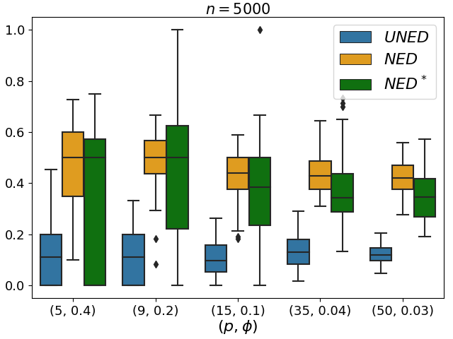
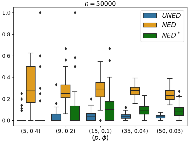
4.2 Estimating DAGs for XSCMs with cross-sectional data
To initialize an XSCM for the vector , we randomly generate a path coefficient matrix with a predefined sparsity level . For simplicity, we assume that the components in are topologically ordered, so that the corresponding path coefficient matrix is a lower triangular matrix (see Appendix B.1). Specifically, for each , the entry is set to zero with probability , and otherwise sampled uniformly on the interval . The associated DAG, , is then constructed with vertex set and directed edge set . The left panel of Figure 1 shows an example of a randomly initialized , while the right panel illustrates the corresponding DAG.
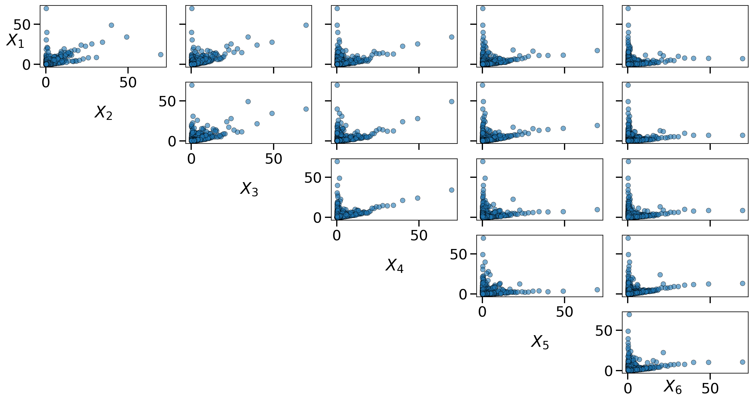
Given the initialized XSCM, independent samples are generated using the direct form where the source variables, , are simulated as described in Section 4.1; illustrative scatter plots of samples generated from the XSCM are shown in Figure 7 of Appendix A.1.
To examine the effect of the number of variables , the connectivity level , and the sample size , on graph recovery, we test our method under various combinations. The expected number of edges, , ranges from 5 to 70. The results are shown in Figure 2, with the left panel showing the method’s performance with a small sample size () and the right with a large sample size (). When ignoring edge directions (UNED), our method performs consistently well, indicating reliable skeleton recovery. When directions are considered (NED and NED∗), the error increases. Notably, NED∗ improves with larger sample sizes, whereas NED does not. This is consistent with the discussion in Section 2.2, where we highlight that different Markov equivalent DAGs can share the same skeleton and separation sets, leading to ambiguity in direction recovery.
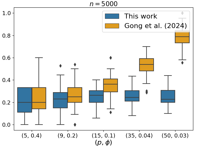
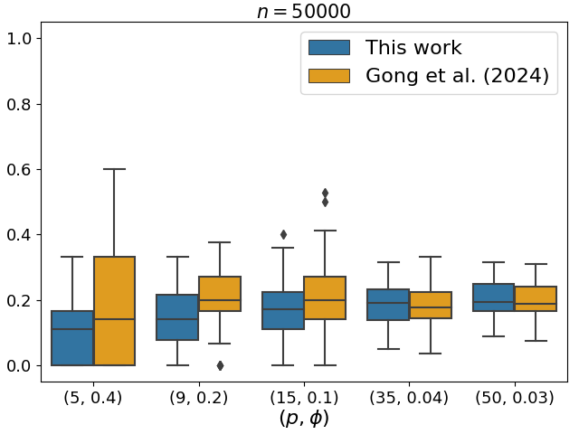
4.3 Estimating the undirected graph of extremal Markov networks
To initialize an extremal Markov network for , we first generate a precision matrix with varying levels of sparsity , where denotes the TPDM of . To ensure that is symmetric, positive-definite and non-negative, we require to be a symmetric, non-singular -matrix (see Appendix B.1). Specifically, we set each entry , with , to zero with probability , and otherwise draw it from a uniform distribution over . We then set each diagonal entry to be strictly greater than the maximum absolute value of its corresponding row and column entries. The associated undirected graph is then defined with vertex set and edge set .
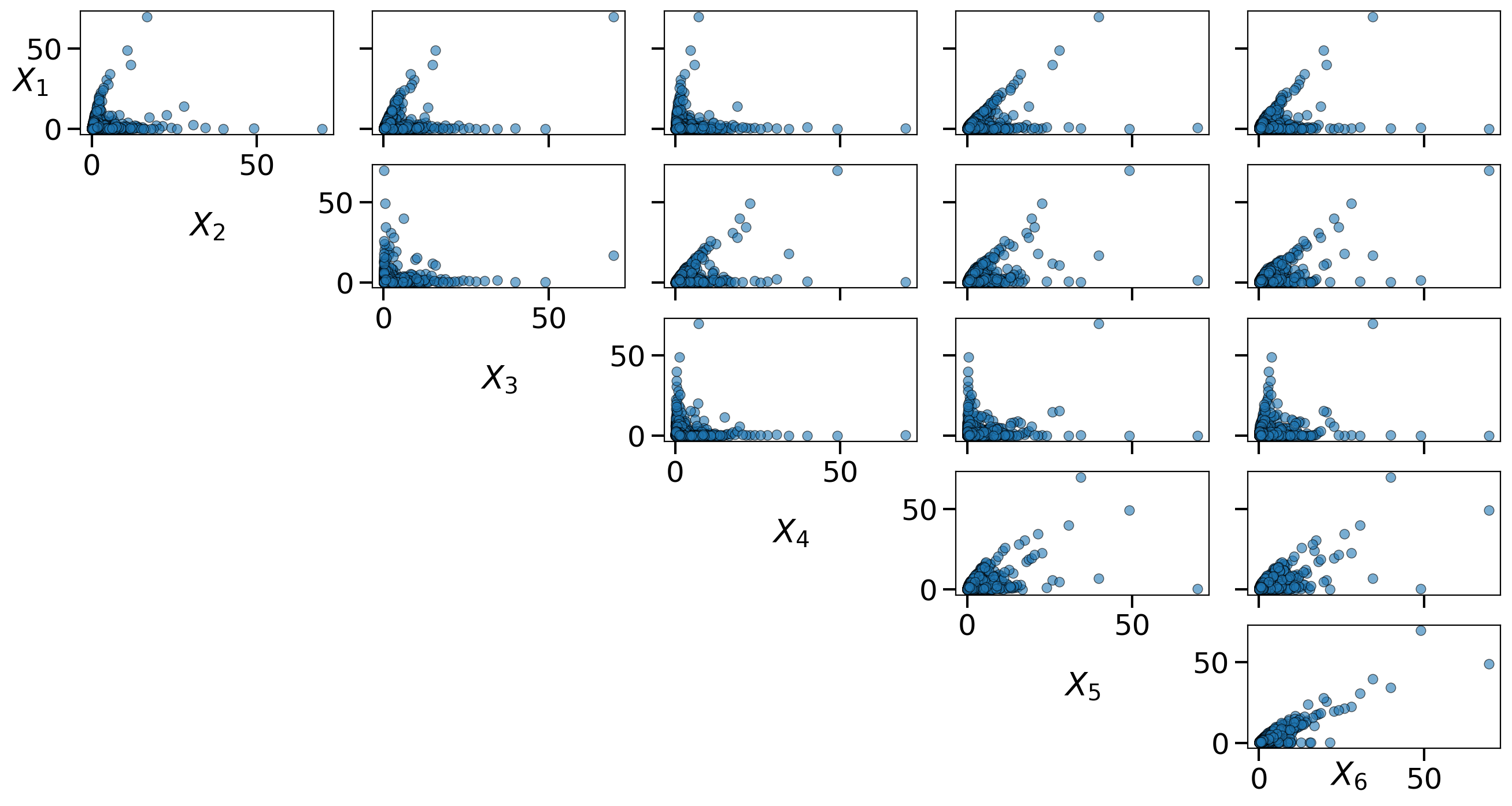
To generate samples from the extremal Markov network , we use the transformation , where is the lower triangular matrix from the Cholesky decomposition of and is simulated as described in Section 4.1. An illustration of an extremal Markov network and the corresponding simulated samples are shown in Appendix A.2.
Results under varying combinations of scale and connectivity parameters , and two different sample sizes, are summarized in Figure 3. The results indicate that our method generally outperforms that proposed by Gong et al., (2024), particularly under high dimensionality and small sample size. The reason why our method generally performs better is that the approach of Gong et al., (2024) relies on the pairwise Markov property, which requires conditioning on all other variables as the separation set. In contrast, our method only needs to identify a often much smaller separation set. Conditioning on an unnecessarily large set can introduce noise, making the test less data-efficient and reducing practical performance.
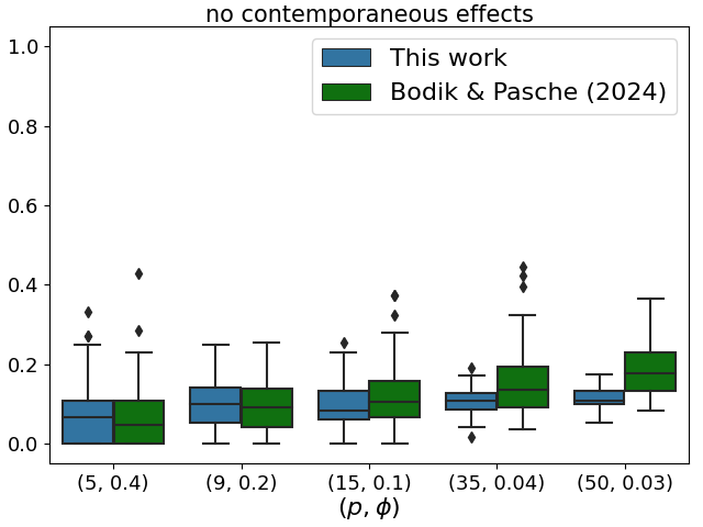
4.4 Estimating DAGs for XSCMs from time series data
Initialization of the XSCM for time series follows the same procedure as with the cross-sectional case. To ensure acyclicity within each time slice, is constrained to be lower triangular, while the lagged matrices have no such constraints. We control the overall sparsity level using a connectivity parameter , and draw non-zero entries uniformly on . The corresponding graph is constructed with and . Then, the time series is generated iteratively using (8). See Appendix A.3, for an example.
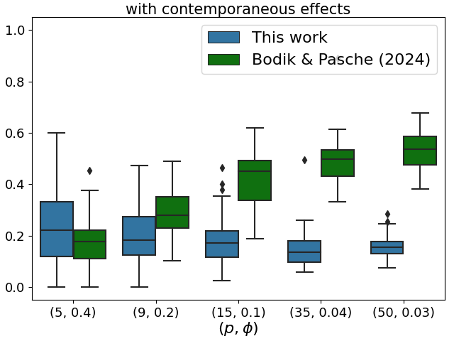
We consider a maximum lag and simulate time points for different XSCMs time series. As the method proposed by Bodik and Pasche, (2024) cannot capture contemporaneous causal effects, we conduct two sets of experiments. In the first, we impose (the zero matrix) to remove contemporaneous effects. In the second, is allowed to contain non-zero entries. We apply both our method and the method of Bodik and Pasche, (2024) to estimate the underlying DAGs, evaluating performance using the normalized edit distance defined in Equation (9), while ignoring edges associated with contemporaneous effects.
Results under varying combinations of scale and connectivity parameters are summarized in Figure 4. The left panel shows the method’s performance under , and the right panel shows the performance when contemporaneous effects are accounted for. When is zero, our method performs better than Bodik and Pasche, (2024) but with a small margin. However, once contemporaneous effects are introduced, the performance of the method in Bodik and Pasche, (2024) deteriorates significantly, while our method remains robust. The performance gap increases with the number of variables, .
5 Real data applications
This section presents two applications of our proposed method. Section 5.1 demonstrates the estimation of the underlying DAG structure in the Danube river basin dataset, a well-known benchmark application in hydrology and widely used in the literature on graphical modeling for extremes (see, e.g., Asadi et al.,, 2015; Engelke and Hitz,, 2020; Lee and Cooley,, 2022; Gong et al.,, 2024; Bodik and Pasche,, 2024). Section 5.2 investigates causal discovery in trading activities of China’s future market, based on a high-frequency financial dataset constructed by Jiang et al., (2024).
5.1 Danube river basin data
The Danube river basin dataset contains daily discharge data from 31 gauging stations along the Danube river basin spanning the period from 1960 to 2009. We use the preprocessed version provided by Asadi et al., (2015), which includes only summer months (June, July, August), resulting in a total of observations. The known river topology is shown in the upper panel of Figure 5, where edge directions indicate flow from upstream to downstream.
To satisfy the regular variation condition in Definition 2.4, we first apply an empirical rank transformation to each margin as described in Section 2.3, resulting in unit Pareto margins with shape parameter 2. We then apply our method to estimate the underlying DAG. The two free hyperparameters are set to . The estimated graphs for maximum causal lags and are shown in the middle-left and middle-middle panels of Figure 5, respectively. In those two graphs, edge thickness is proportional to the PTCC scores. Directed edges indicate identifiable causal directions; undirected edges represent dependencies with unidentifiable directions. Red edges denote one-step lagged causal effects.
When lagged effects are excluded (, middle-left), our method successfully recovers most of the skeleton of the river structure, although many contemporaneous directions remain unidentified. When incorporating one-step lagged causality (, middle-middle), directionality estimation improves. For example, a collider structure is detected at station 7. Additionally, one-step lagged causal connections are identified between stations 3 and 4, and between stations 25 and 27—both of which are consistent with the known river topology.
To facilitate comparison, we also present results from several existing methods applied to the same dataset. In Engelke and Hitz, (2020), results assuming that the underlying structure is a tree or an undirected graph are shown in the middle-right and bottom-left panels of Figure 5, respectively. The former achieves better performance than the latter, as it is a stronger assumption than assuming that the underlying structure is a general undirected graph. The results by Lee and Cooley, (2022) and Gong et al., (2024) are shown in the bottom-middle and bottom-right panels, respectively. Overall, our method offers greater expressiveness and interpretability by learning the DAG structure, and it is more general, being applicable to time series data.
5.2 Tail causality in China’s future market
We now also apply our method to high-frequency trading data from China’s future market, which constitutes a subset of the time series dataset constructed by Jiang et al., (2024). Our analysis focuses on tail causal discovery in trading activities during the period from 2024-02-28 to 2025-02-28. The dataset covers products across various categories, from traditional commodities such as grains and coal to financial instruments like equity index and interest rate futures, as listed in Table 1 with their categories. For details on the specific assets represented by each product code, please refer to the Jiang et al., (2024), Section B of the Supplementary Material. Trading activity is measured as the aggregated trading volume over 5-minute intervals, normalized by the total daily volume, yielding observations in total.
We apply the marginal transformation described in Section 5.1 to satisfy the regular variation condition. Our method is then applied fixing the hyperparameters as , and maximum causal lag as . The resulting causal graph is shown in Figure 6, where the edge widths are proportional to the PTCC scores. To better visualize the structure, we cluster the assets based on the PTCC scores for contemporaneous relationships using the -means algorithm. The number of clusters is set to , corresponding to the number of categories in Table 1.
| Category | Codes | Category | Codes |
|---|---|---|---|
| Oil crops | a, m, OI, p, b, RM, y | Precious metals | ag, au |
| Nonferrous metals | al, bc, cu, ni, pb, sn, zn, ao | Economic crops | AP, CF, CJ, CY, PK, SR |
| Rubber & woods | br, fb, nr, ru, sp | Oil & gas | bu, fu, lu, pg, sc |
| Grains | c, cs | Olefins | eb, l, pp, v |
| Alcohols | eg, MA | Inorganics | FG, SA, UR, SH |
| Ferrous metals | hc, i, rb, SF, SM, ss | Equity index | IC, IF, IH, IM |
| Coals | j, jm | Animals | jd, lh |
| Novel materials | lc, si | Aromatics | PF, TA, PX |
| Interest rates | T, TF, TL, TS | Indices | ec |
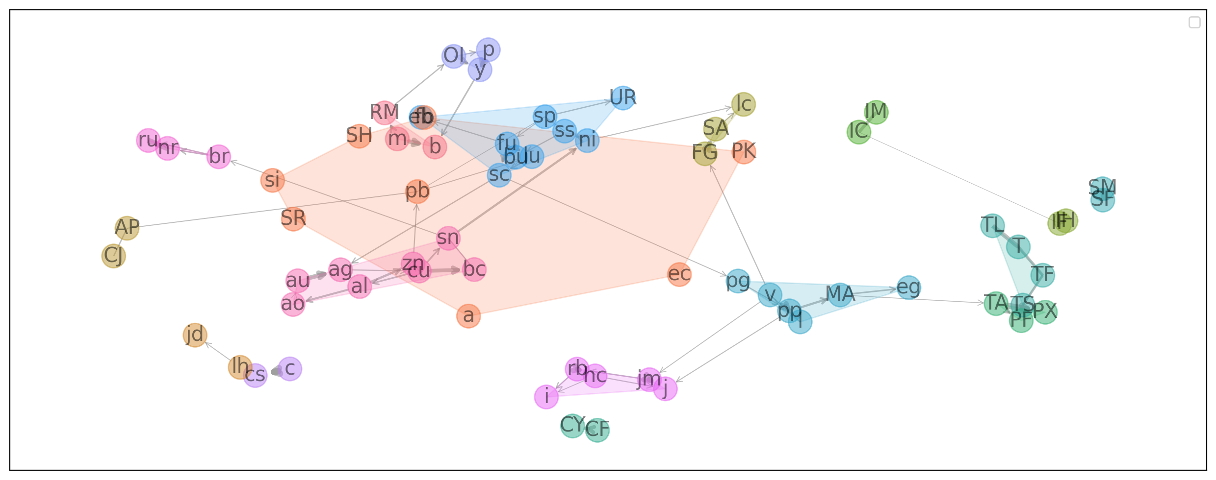
The results indicate that large trading activity tends to be more strongly associated with large trading activity within the same product category. For example, the national bond futures—T, TL, TS, and TF—exhibit strong contemporaneous connections. Similar patterns are observed in agricultural products (OI, p, y, RM, m, b) and chemical products (TA, PF, PX). Furthermore, thanks to the collider structure identified by our method, partial directionality can be inferred even in contemporaneous relationships. Examples include lhjd, auag, among others. We find that the direction of edges tend to originate from assets with higher trading activity. Specifically, by comparing the daily average trading turnover (measured in USD) for each pair of directed edges, we observe that in out of the pairs, the asset identified as the cause has a larger trading turnover than the effect asset.
6 Conclusion
We have introduced a new structural causal model—the XSCM—to capture causal direction in tail-dependent (and potentially heavy-tailed) data. Our main theoretical contribution is the establishment of an equivalence between zero PTCC and graph separation, applicable to both XSCMs and extremal Markov networks. This equivalence allows the problem of learning both DAG structures (in XSCMs) and undirected structures (in extremal Markov networks) to be reformulated as separation detection in graphs, making the use of popular constraint-based learning algorithms applicable.
To evaluate the efficiency of our method, we conducted simulation studies in three distinct settings: inferring DAGs from cross-sectional data, inferring DAGs from time series data, and estimating undirected graph structures. In all cases, our method achieves strong performance compared to existing approaches. We further demonstrated the practical value of our method through two real-world applications. For the Danube river basin dataset, our method successfully recovers the known river topology and identifies collider structures and lagged causal relationships. In the high-frequency trading data application from China’s futures market, the learned graph structure aligns well with product categories, capturing both within-category dependence and partial directionality in extremal trading activity.
In parallel work, the recent preprint of Engelke et al., (2025) derived an extremal SCM by analyzing the limiting tail behavior of classical SCMs. Although both works independently tackle causality in extremes through SCMs, the two proposed frameworks remain distinct, and it would be interesting in future research to study their respective strengths and limitations. One of the key differences is that our approach directly constructs a new causal framework tailored to extremes, rather than deriving it from asymptotic arguments, and thus it provides a foundation for structure learning in this setting. Another possible direction for future research is to study the causal mechanisms of extreme events that occur in both directions of a random variable. Modeling such mechanisms—where extremes may arise in both the upper and lower tails—is receiving increasing attention in the literature; see, for example, Gnecco et al., (2021) and Bodik and Pasche, (2024), where the variable of interest is transformed by taking its absolute value so that existing methods can be applied. However, given the growing acknowledgment of the differing behaviors in the joint upper and lower tail regions, as well as evidence of complex cross-directional dependence (Jiang et al.,, 2024), explicitly modeling the interaction between the upper and lower tails is increasingly necessary. This challenge calls for the development of new structural causal models that account for the inherent constraint between the two tails of the same variable, and may open up a promising line of research.
Competing interests
No competing interest is declared.
Acknowledgments
The author gratefully acknowledges valuable discussions with Dr. Nabila Bounceur on state-of-the-art causal discovery methods.
References
- Asadi et al., (2015) Asadi, P., Davison, A. C., and Engelke, S. (2015). Extremes on river networks. The Annals of Applied Statistics, 9(4):2023–2050.
- Berman, (1994) Berman, A. (1994). Nonnegative Matrices in the Mathematical Sciences. Society for Industrial and Applied Mathematics.
- Bodik et al., (2024) Bodik, J., Paluš, M., and Pawlas, Z. (2024). Causality in extremes of time series. Extremes, 27(1):67–121.
- Bodik and Pasche, (2024) Bodik, J. and Pasche, O. (2024). Granger causality in extremes. arXiv preprint arXiv:2407.09632.
- Chavez-Demoulin and Mhalla, (2024) Chavez-Demoulin, V. and Mhalla, L. (2024). Causality and extremes. arXiv preprint arXiv:2403.05331.
- Colombo et al., (2012) Colombo, D., Maathuis, M. H., Kalisch, M., and Richardson, T. S. (2012). Learning high-dimensional directed acyclic graphs with latent and selection variables. The Annals of Statistics, 40(1):294–321.
- Cooley and Thibaud, (2019) Cooley, D. and Thibaud, E. (2019). Decompositions of dependence for high-dimensional extremes. Biometrika, 106(3):587–604.
- Cormen and Leiserson, (2022) Cormen, T. H. and Leiserson, C. E. (2022). Introduction to Algorithms. MIT Press, fourth edition.
- Engelke et al., (2025) Engelke, S., Gnecco, N., and Röttger, F. (2025). Extremes of structural causal models. arXiv preprint arXiv:2503.06536.
- Engelke et al., (2024) Engelke, S., Hentschel, M., Lalancette, M., and Röttger, F. (2024). Graphical models for multivariate extremes. arXiv preprint arXiv:2402.02187.
- Engelke and Hitz, (2020) Engelke, S. and Hitz, A. S. (2020). Graphical models for extremes. Journal of the Royal Statistical Society Series B: Statistical Methodology, 82(4):871–932.
- Engelke and Ivanovs, (2021) Engelke, S. and Ivanovs, J. (2021). Sparse structures for multivariate extremes. Annual Review of Statistics and Its Application, 8(1):241–270.
- Engelke and Volgushev, (2022) Engelke, S. and Volgushev, S. (2022). Structure learning for extremal tree models. Journal of the Royal Statistical Society: Series B (Statistical Methodology), 84(5):2055–2087.
- Gnecco et al., (2021) Gnecco, N., Meinshausen, N., Peters, J., and Engelke, S. (2021). Causal discovery in heavy-tailed models. The Annals of Statistics, 49(3):1755–1778.
- Gong et al., (2024) Gong, Y., Zhong, P., Opitz, T., and Huser, R. (2024). Partial tail-correlation coefficient applied to extremal-network learning. Technometrics, 66(3):331–346.
- Hammoudeh et al., (2020) Hammoudeh, S., Ajmi, A. N., and Mokni, K. (2020). Relationship between green bonds and financial and environmental variables: A novel time-varying causality. Energy Economics, 92:104941.
- Hill, (1975) Hill, B. M. (1975). A simple general approach to inference about the tail of a distribution. The Annals of Statistics, pages 1163–1174.
- Imai et al., (2013) Imai, K., Tingley, D., and Yamamoto, T. (2013). Experimental designs for identifying causal mechanisms. Journal of the Royal Statistical Society Series A: Statistics in Society, 176(1):5–51.
- Isaacson, (1994) Isaacson, E. (1994). Analysis of Numerical Methods. Dover Publications.
- Jiang et al., (2024) Jiang, J., Richards, J., Huser, R., and Bolin, D. (2024). The efficient tail hypothesis: An extreme value perspective on market efficiency. arXiv preprint arXiv:2408.06661.
- Klüppelberg and Krali, (2021) Klüppelberg, C. and Krali, M. (2021). Estimating an extreme Bayesian network via scalings. Journal of Multivariate Analysis, 181:104672.
- Krali, (2025) Krali, M. (2025). Causal discovery in heavy-tailed linear structural equation models via scalings. arXiv preprint arXiv:2502.13762.
- Krali et al., (2023) Krali, M., Davison, A. C., and Klüppelberg, C. (2023). Heavy-tailed max-linear structural equation models in networks with hidden nodes. arXiv preprint arXiv:2306.15356.
- Lee and Cooley, (2021) Lee, J. and Cooley, D. (2021). Transformed-linear prediction for extremes. arXiv preprint arXiv:2111.03754.
- Lee and Cooley, (2022) Lee, J. and Cooley, D. (2022). Partial tail correlation for extremes. arXiv preprint arXiv:2210.02048.
- Paluš et al., (2024) Paluš, M., Chvosteková, M., and Manshour, P. (2024). Causes of extreme events revealed by rényi information transfer. Science Advances, 10(30).
- Pasche et al., (2023) Pasche, O. C., Chavez-Demoulin, V., and Davison, A. C. (2023). Causal modelling of heavy-tailed variables and confounders with application to river flow. Extremes, 26(3):573–594.
- Pearl, (2009) Pearl, J. (2009). Causality: Models, Reasoning, and Inference. Cambridge University Press, Cambridge, UK, 2nd edition.
- Pearl, (2014) Pearl, J. (2014). Probabilistic Reasoning in Intelligent Systems: Networks of Plausible Inference. Elsevier.
- Peters et al., (2017) Peters, J., Janzing, D., and Schölkopf, B. (2017). Elements of Causal Inference: Foundations and Learning Algorithms. The MIT Press.
- Resnick, (2007) Resnick, S. I. (2007). Heavy-tail Phenomena: Probabilistic and Statistical Modeling. Springer Science & Business Media.
- Rue and Held, (2005) Rue, H. and Held, L. (2005). Gaussian Markov Random Fields: Theory and Applications. Chapman and Hall/CRC.
- Runge, (2018) Runge, J. (2018). Causal network reconstruction from time series: From theoretical assumptions to practical estimation. Chaos: An Interdisciplinary Journal of Nonlinear Science, 28(7):075310.
- Runge, (2020) Runge, J. (2020). Discovering contemporaneous and lagged causal relations in autocorrelated nonlinear time series datasets. In Conference on Uncertainty in Artificial Intelligence, pages 1388–1397. PMLR.
- Runge et al., (2015) Runge, J., Petoukhov, V., Donges, J. F., Hlinka, J., Jajcay, N., Vejmelka, M., Hartman, D., Marwan, N., Paluš, M., and Kurths, J. (2015). Identifying causal gateways and mediators in complex spatio-temporal systems. Nature Communications, 6(1):8502.
- Shojaie and Fox, (2022) Shojaie, A. and Fox, E. B. (2022). Granger causality: A review and recent advances. Annual Review of Statistics and Its Application, 9:289–319.
- Spirtes, (2001) Spirtes, P. (2001). An anytime algorithm for causal inference. In International Workshop on Artificial Intelligence and Statistics, pages 278–285. PMLR.
- Spirtes et al., (2000) Spirtes, P., Glymour, C. N., and Scheines, R. (2000). Causation, Prediction, and Search. MIT press.
Appendix A More on simulation
A.1 More on estimating DAGs for XSCMs with cross-sectional data
A.2 More on estimating the undirected graph of extremal Markov network
Figure 8 shows an example of a randomly initialized precision matrix (left panel) and its corresponding undirected graph structure (right panel).
Figure 9 presents the pairwise scatter plots of samples generated from the extremal Markov network in Figure 8.
A.3 More on estimating DAGs for XSCMs from time series data
Figure 10 (left) shows an example of randomly initialized and for a 3-dimensional time series with lag , and the right panel illustrates the corresponding DAG.
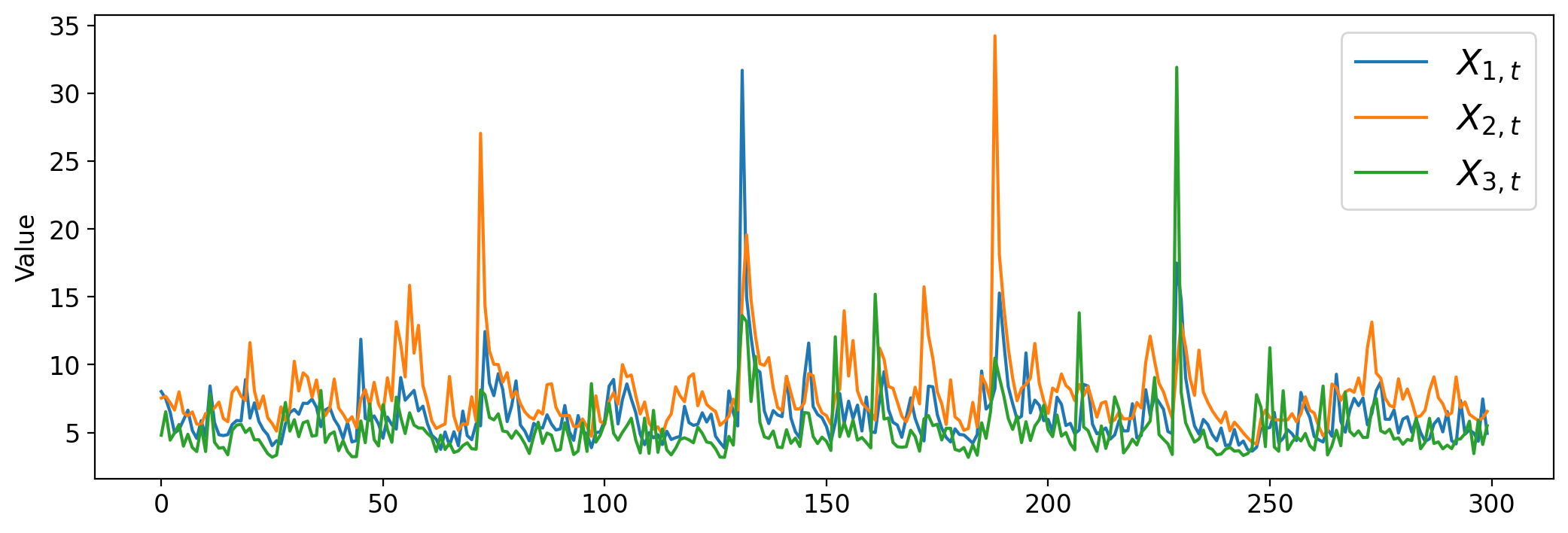
Figure 11 displays the simulated trajectory (length ) corresponding to the XSCM in Figure 10, where occurrences of extreme values can be observed across multiple variables at the same time.
Appendix B Proofs
B.1 Proof of Proposition 3.1
Proof of Proposition 3.1.
We first prove that is invertibe and that its inverse, is a non-negative matrix. Assuming this holds, the direct calculation
shows that . For any matrix , the TPDM for is where masks the negative values in (Cooley and Thibaud,, 2019, Sec. 4). Courtesy of the non-negativity of , we obtain
where the is the scale matrix of the XSCM.
Now, to prove the invertibility and non-negativity of , we first reorder the random vector and using topological ordering, which is a bijective mapping that satisfies whenever . For any DAG , a topological ordering always exists (Peters et al.,, 2017; Proposition B.2 and Cormen and Leiserson,, 2022; Theorem 20.12). Let be the row swapping matrix for topological ordering, i.e., for and all other elements are zero. Define the reordered random vector , and its corresponding reordered source variables by . Rewriting and using and , we have that
The corresponding reordered path coefficient matrix is and the scale matrix is for and . By the definition of topological ordering, is a strict lower triangular matrix. Consequently, is a convergent matrix, i.e., , and has a spectral radius (Isaacson,, 1994, Theorem 4.c). Since and are similar matrices, the path coefficient matrix is also convergent.
For a convergent matrix , the matrix is invertible and can be expressed as a Neumann series: (Isaacson,, 1994, Theorem 5). Since is non-negative, remains non-negative for all , implying that is also non-negative. ∎
Remark.
An alternative proof is to show that is a nonsingular -type matrix (Berman,, 1994, Definition 1.2). A nonsingular -type matrix is a square matrix in the form where for . An -type matrix is invertible and its inverse is positive. After deriving , we readily notice that is a nonsingular -type matrix.
B.2 Proof of Proposition 3.2
Lemma B.1.
For any XSCM for with underlying graph and , there exists a Gaussian linear causal model for , where the source variables are independent and identically distributed Gaussian random variables. The model shares the same graph structure and the same path coefficient matrix and scale matrix as . Moreover, the direct representation of is .
Proof of Proposition 3.2.
For any XSCM for , where , let for be the corresponding Gaussian linear causal model as stated in Lemma B.1. They share the same underlying graph structure and the same path coefficient matrix and scale matrix as . The system is a linear function of and follows a joint Gaussian distribution.
It is well established that Gaussian linear structural causal models satisfy both the causal Markov and causal faithfulness conditions (Spirtes et al.,, 2000, Proposition 6.31 and Theorem 3.2). Consequently, for any two vertices and , vertices and are d-separated by if and only if the conditional covariance , where .
Furthermore, the conditional covariance has the same form as the partial tail-covariance where . Therefore, for any and , if and only if where . This equivalence establishes both the tail-causal Markov and tail-causal faithfulness properties for XSCM. ∎
B.3 Proof of Proposition 3.3
Proof of Proposition 3.3.
Given a random vector with where are independent and identically-distributed regularly varying random variables with tail index . Let . The TPDM of is given by and the induced undirected graph is .
Let a corresponding random vector with . The vector is a Gaussian Markov random field (Rue and Held,, 2005, Definition 2.1) with regards to the same underlying undirected graph for the extremal Markov network . Furthermore, the covariance matrix for is given by . For Gaussian Markov random fields, the equivalence between the global Markov property and the pairwise Markov property are established (Rue and Held,, 2005, Theorem 2.4). Also, for any two vertces and a separation set , the conditional covariance equals the partial tail-covariance , where and . For a joint Gaussian random vector, the conditional covariance equals zero if and only if conditional independence holds. Therefore, the two vertices are separated by if and only if PTCC for . This concludes the proof. ∎
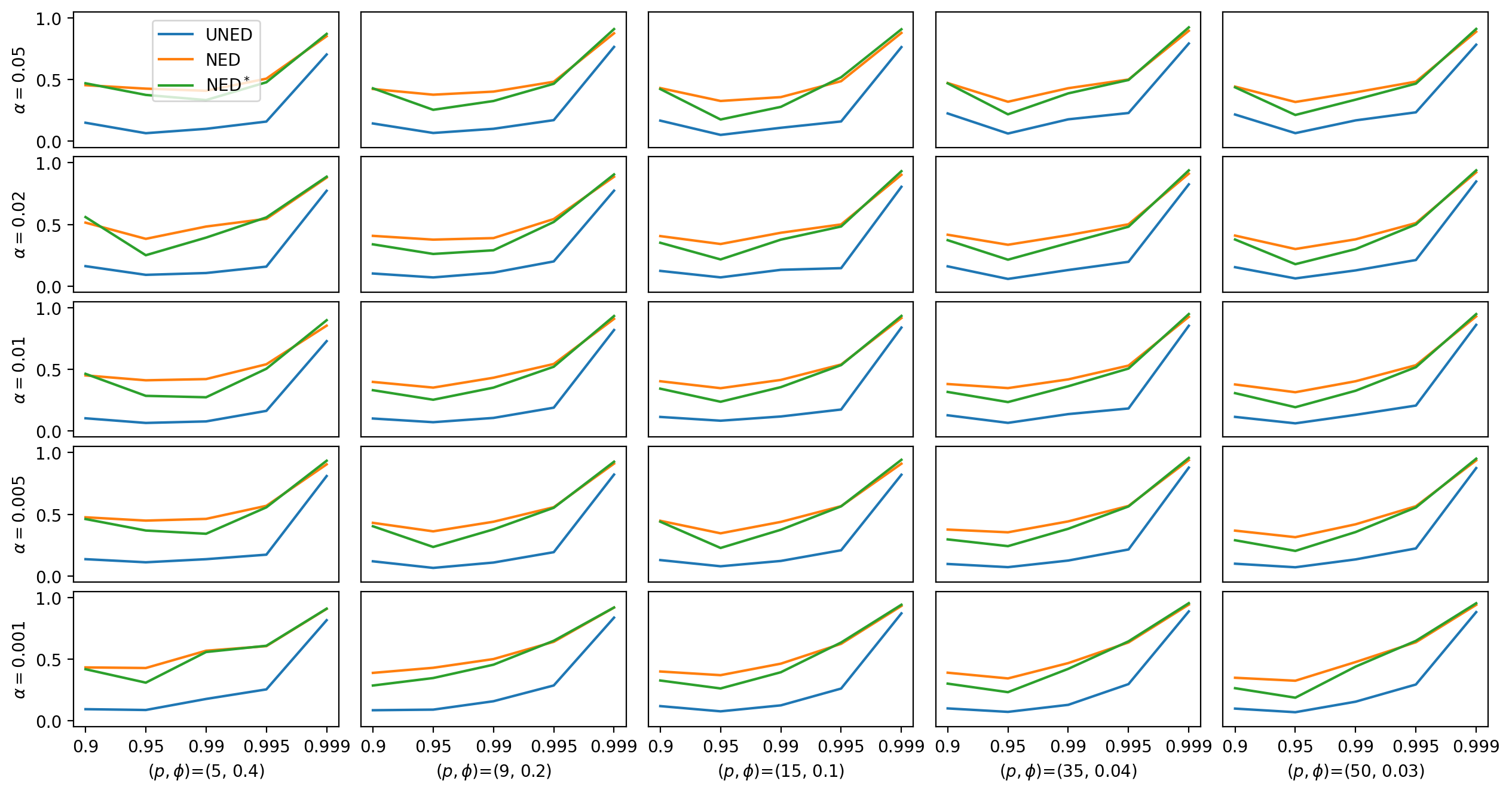
Appendix C Sensitivity analysis
To investigate the sensitivity of the DAG estimation to the choice of hyperparameters and , we consider the scenario of estimating the DAG of an XSCM model using cross-sectional data. We conduct experiments under different settings of the number of variables and sparsity level , and report the recovery performance—measured by UNED, NED, and NED∗—across various choices of and . Figure 12 presents the results. The performance is not sensitive to the significance level , and it remains stable with respect to the quantile when is close to 1.