JWST Observations of Young protoStars (JOYS)

Abstract

Context. The embedded phase of star formation is a crucial period in the development of a young star as the system still accretes matter, emerges from its natal cloud assisted by powerful jets and outflows, and forms a disk setting the stage for the birth of a planetary system. Mid-infrared spectral line observations, now possible with unprecedented sensitivity, spectral resolution and sharpness with the James Webb Space Telescope (JWST), are key for probing many of the physical and chemical processes on sub-arcsecond scales that occur in highly extincted regions, providing unique diagnostics and complementing millimeter observations.

Aims. The JWST Observations of Young protoStars (JOYS) program aims to address a wide variety of questions, ranging from protostellar accretion and the nature of primeval jets, winds and outflows, to the chemistry of gas and ice in hot cores and cold dense protostellar environments, and the characteristics of the embedded disks. We introduce the program and show representative JOYS results.

Methods. JWST Mid-InfraRed Instrument (MIRI) Medium Resolution Spectrometer (MRS) Integral Field Unit (IFU) 5–28 $\mu$m maps of 17 low-mass targets (23 if binary components counted individually) and 6 high-mass protostellar sources are taken with resolving powers $R=\lambda/\Delta\lambda=1500-4000$. Small mosaics ranging from $1\times 1$ to $3\times 3$ MRS tiles cover $\sim 4^{\prime\prime}$ to $20^{\prime\prime}$ fields of view, providing spectral imaging on spatial scales down to $\sim$30 au (low mass) and $\sim$600 au (high mass). For HH 211, the complete $\sim 1^{\prime}$ blue outflow lobe has been mapped with the MRS. Atomic lines are interpreted with published shock models, whereas molecular lines are analyzed with simple rotation diagrams and LTE slab models. The importance of taking infrared pumping into account is stressed. Inferred abundance ratios are compared with detailed hot core chemical models including X-rays. Ice spectra are fitted through comparison with laboratory spectra.

Results. The JWST MIRI-MRS spectra show a wide variety of features, with their spatial distribution providing insight into their physical origin. Atomic line maps differ among refractory (e.g., Fe), semi-refractory (e.g., S) and volatile elements (e.g., Ne), and are linked to their different levels of depletion and local (shock) conditions. Jets are prominently seen in lines of [Fe II] and other refractory elements whereas the pure rotational H₂ lines probe hot ($\sim 1000$ K) and warm (few$\times 10^{2}$ K) gas inside the cavity, associated with jets, outflows and cavity walls, for both low- and high-mass sources. Wide-angle winds are found in low-$J$ H₂ lines. Nested, stratified jet structures consisting of an inner ionized core with an outer molecular layer are commonly seen in the youngest sources. [S I] follows the jet as seen in [Fe II] in the youngest protostars, but is different in more evolved sources where it is concentrated on source. Noble gas lines such as [Ne II] 12.8 $\mu$m reveal a mix of jet shock and photoionized emission. H I recombination lines serve as a measure of protostellar accretion rates, but are also associated with more extended jets. Gaseous molecular emission (CO₂, C₂H₂, HCN, H₂O, CH₄, SO₂, SiO) is seen toward several sources, but is cool compared with what is found in more evolved disks, with excitation temperatures of only 100–250 K, and likely associated with the warm inner envelopes (“hot cores”) . CO₂ is often extended along the outflow, in contrast with C₂H₂ which is usually centered on source. Water emission is commonly detected on source even if relatively weak; off source it is seen only in the highest density shocks such as associated with NGC 1333 IRAS4B. Some sources show gaseous molecular lines in absorption, including NH₃ in one case. Deep ice features are seen toward the protostars, revealing not just the major ice components but also ions (as part of salts) and complex organic molecules, with comparable abundances from low- to high-mass sources. Relative abundances of some gas and ice species are similar, consistent with ice sublimation in hot cores. A second detection of HDO ice in a solar-mass source is presented, with an HDO/H₂O ice ratio of $\sim$0.4%, providing a link with HDO/H₂O in disks and comets. A deep search for solid O₂ suggests that it is not a significant oxygen reservoir. Only few embedded Class I disks show the same forest of water lines as Class II disks do, possibly caused by significant dust extinction of the upper layers due to limited growth and settling of dust to the midplane in young disks as well as radial drift bringing in small dust.

Conclusions. This paper illustrates the many different science questions that a single MIRI-MRS IFU data set can address, with significant similarities between low- and high-mass sources. Large source samples across evolutionary stages and luminosities are needed to further develop these diagnostics of the physics and chemistry of protostellar systems.

1 Introduction

The embedded phase of star formation, typically up to a few $\times 10^{5}$ yr after cloud collapse, is a critical and highly active period in the evolution of a young stellar object when it gathers most of its mass and is emerging from its dense environment (André et al., 2000; Evans et al., 2009; Dunham et al., 2014; Fischer et al., 2017). Besides accretion onto the main core, many other physical processes occur simultaneously in the immediate surroundings of the protostar: infall from the natal cloud and collapsing envelope onto the young disk, jets and winds ejected from the star-disk system, outflows sweeping up and shocking the material, and ultraviolet (UV) photons and X-rays heating, ionizing and dissociating the gas (e.g., Arce et al., 2007; Bally, 2016; Tobin & Sheehan, 2024). Young disks are massive and still spreading radially (e.g., Hueso & Guillot, 2005; Ohashi et al., 2023), with planet formation already starting at this early stage (Manara et al., 2018; Tychoniec et al., 2020). Chemical processes range from freeze-out and ice chemistry in the cold outer parts to ice sublimation and high temperature chemistry in “hot cores” and shocks (e.g., van Dishoeck & Blake, 1998; Jørgensen et al., 2020; Ceccarelli et al., 2023). Ultimately, the early pre- and protostellar stages provide the chemical building blocks of disks, comets and planets (e.g., Caselli et al., 2012; Öberg & Bergin, 2021).

Because of tens to hundreds of magnitudes of visual extinction in the inner regions, however, these processes and materials can often only be probed at infrared (IR) and millimeter-centimeter wavelengths. The Atacama Large Millimeter/submillimeter Array (ALMA) has allowed protostellar systems to be imaged in the warm and cold(er) molecular gas and dust continuum at subarcsec scales, probing their physical and chemical structure (e.g., Tobin & Sheehan, 2024). However, many key processes, traced by diagnostic lines of warm-to-hot (shocked) gas and of solid state material, can only be observed at mid- and far-infrared wavelengths.

Pre-JWST mid- and far-infrared observations with the Infrared Space Observatory (ISO), the Spitzer Space Telescope, the Herschel Space Observatory and ground-based facilities (e.g., VLT, Keck, IRTF) have made great progress in finding and characterizing protostars (e.g., Furlan et al., 2008; Evans et al., 2009; Dunham et al., 2014), in using atomic, H₂ and CO lines to probe shock physics (e.g., Rosenthal et al., 2000; Dionatos et al., 2009; Watson et al., 2016; Karska et al., 2018), in tracing H₂O from clouds to disks (e.g. van Dishoeck et al., 2021) and in making an inventory of interstellar ices (e.g., Boogert et al., 2015). However, all of these observations have so far been hampered by either poor spatial resolution, poor spectral resolution and/or low sensitivity. Optical and near-infrared imaging and spectroscopic data from the ground and with HST have provided high spatial and spectral resolution information on jets and outflows, but only in a limited number of tracers at positions with low extinction further away from the source (e.g., McCaughrean et al., 1994; Giannini et al., 2015). While radio observations can probe ionized jets and masers in the inner regions of deeply embedded sources (e.g., Anglada et al., 2018; Ray & Ferreira, 2021; Moscadelli et al., 2022), they lack many other diagnostics. As a result, our understanding of the physical and chemical structure of this early deeply embedded protostellar phase is still incomplete.

The James Webb Space Telescope (JWST) (Rigby et al., 2023; Gardner et al., 2023), in particular its Mid-InfraRed Instrument (MIRI) (Rieke et al., 2015; Wright et al., 2023), allows the next big leap in star formation and protostellar research, bridging the millimeter and near-infrared wavelength regime and providing unique information. MIRI’s spatial resolution of 0.19, 0.58 and 0.96^′′ at 5, 15 and 25 $\mu$m, respectively, corresponds to 29, 87 and 144 au at typical distances of low-mass protostars ($\sim$150 pc, $<10^{2}$ L_⊙) and 570, 1740 and 2800 au at that of high-mass protostars ($\sim$ 3 kpc, $>10^{4}$ L_⊙), well matched to the sizes of their envelopes and disks. The Medium Resolution Spectrometer (MRS) allows mapping capabilities of the inner parts of jets and outflows through its Integral Field Unit (IFU) (Wells et al., 2015; Argyriou et al., 2023). The MRS spectral resolving power of $R=\lambda/\Delta\lambda\sim 1500-4000$ is much higher than that of the Spitzer Space Telescope (which had $R$=50–100 at $<$10 $\mu$m; $R=600$ at $>$10 $\mu$m), boosting line to continuum ratios of gas-phase lines and allowing solid-state bands to be fully resolved. Combined with mJy sensitivity for IFU spectroscopy, this means that the inner parts of collapsing envelopes and outflows of protostars can be dissected on subarcsec scales in the mid-infrared for the first time. Nearly all previous mid-IR spectral line studies were based on single pointings with 5–40^′′ aperture sizes.

The near-infrared spectrograph NIRSpec on JWST (Böker et al., 2023) has similar capabilities as MIRI-MRS but covering the 1–5 $\mu$m range at $R$ up to 2700. Its IFU spectrometer is also well suited for studying the inner regions of protostars at greatly enhanced sensitivity than was possible before (e.g., Federman et al., 2024). Several protostellar studies with JWST, including our program, therefore include both MIRI-MRS 5–28 $\mu$m and NIRSpec-IFU 3–5 $\mu$m data (see references below). This paper focuses almost exclusively on the MIRI data, however.

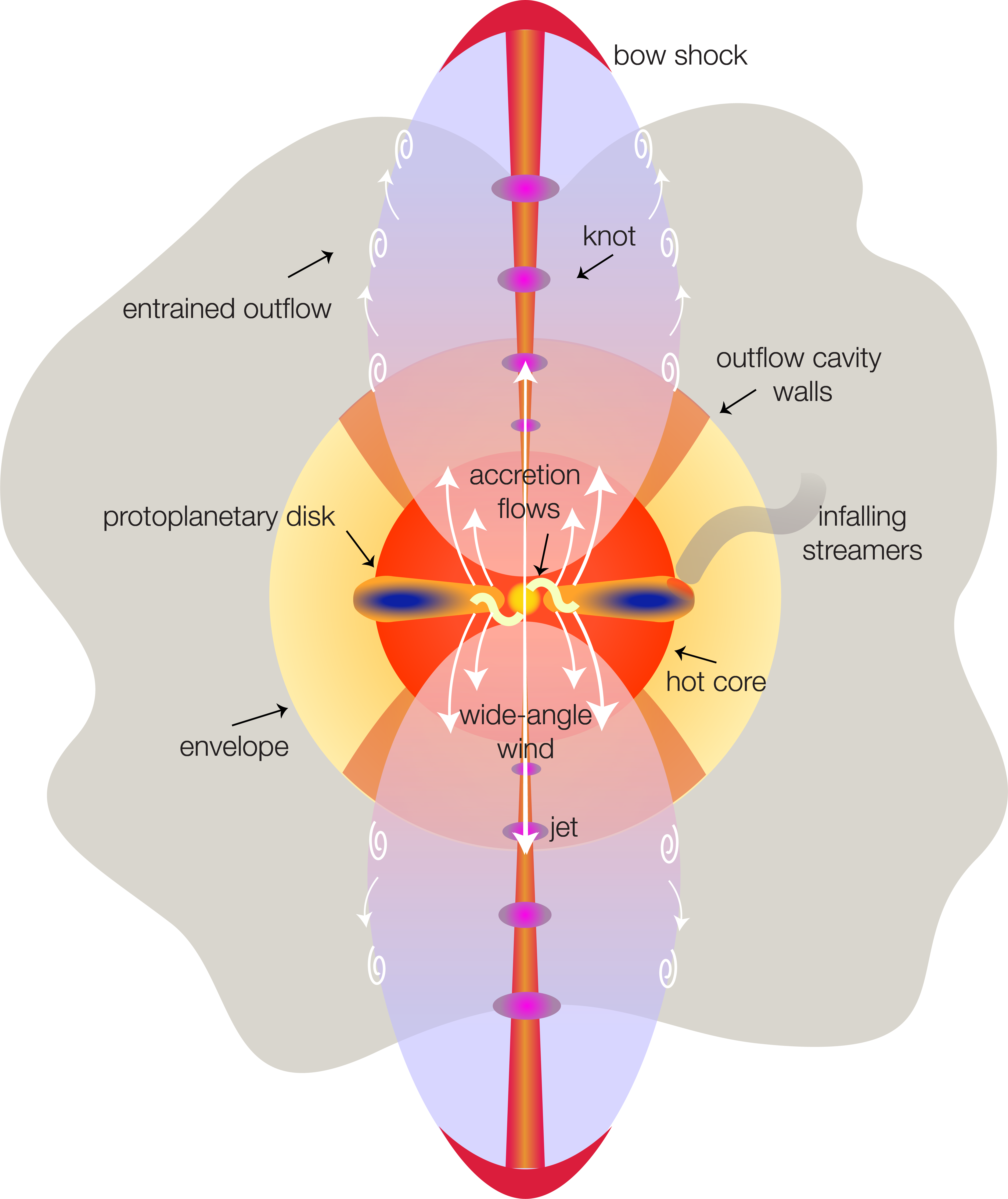
Figure 1: Cartoon of a protostellar source with the various physical components studied in this work indicated.

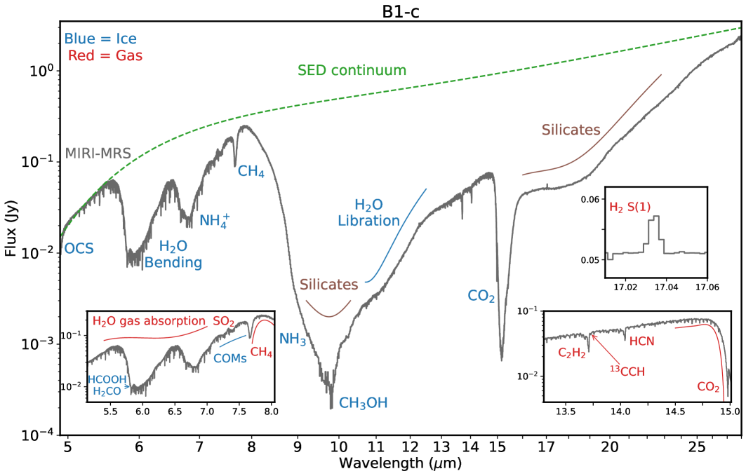
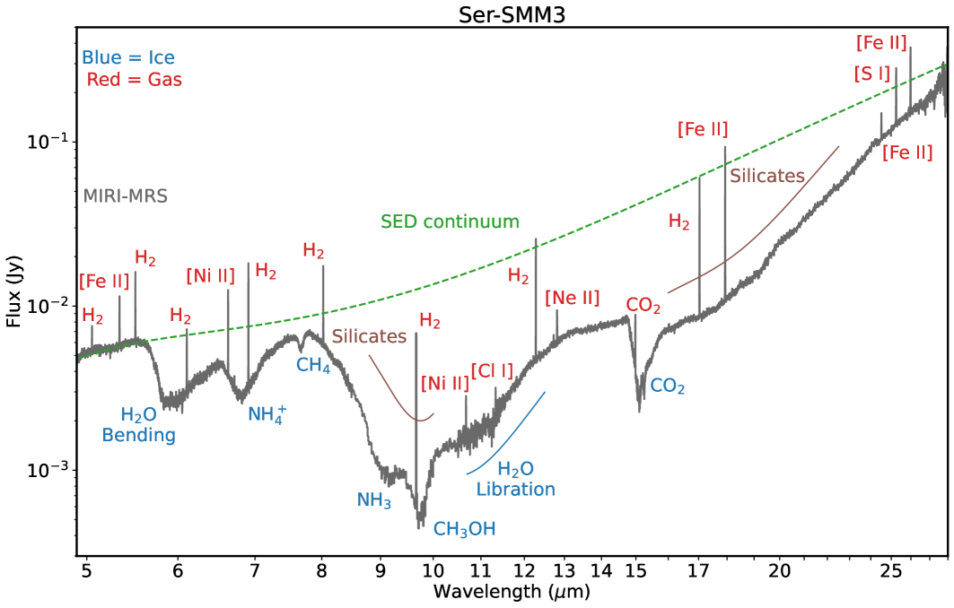
Figure 2: JWST MIRI-MRS spectrum of the low-mass Class 0 protostars B1-c (top) and Serpens SMM3 (bottom) illustrating the different molecular gas (red) and ice (blue) features that can be observed and analyzed, tracing different components of the protostellar system. The inserts in the B1-c spectrum aim to highlight the gas-phase molecular lines in this source. Atomic emission lines are present but not very strong in this source. In contrast, both H₂ and atomic emission lines are very prominent for Serpens SMM3 (bottom). At the bottom of the silicate feature at 10 $\mu$m, close to the noise limit, the spectra have been binned by a factor of 4 to enhance the $S/N$. See Fig. B.3 and B.11 of van Gelder et al. (2024a) for individual MIRI-MRS sub-bands.

In this paper, we outline the MIRI Guaranteed Time Observations (GTO) “JWST Observations of Young protoStars” (JOYS) program centered on MIRI-MRS 5–28 $\mu$m observations of protostellar sources from low ($<$1 L_⊙) to high luminosity ($>10^{4}$ L_⊙), and from the earliest deeply embedded stages where the envelope mass is much larger than the stellar mass (Class 0 for low-mass, Infrared Dark Clouds (IRDCs) for high-mass protostars) to the transitional stage where the star and disk are fully assembled and only a tenuous envelope is left (Class I/II for low-mass protostars) (van Dishoeck et al., 2023; Beuther et al., 2023). Our program 1290 (PI: E.F. van Dishoeck) uses a single observational approach for a set of 23 (17 low-mass + 6 high-mass) protostellar targets (32 if resolved low- and high-mass binary components are counted individually) in order to address the scientific topics listed in § 2.3. For each source, single IFU images or small mosaics (up to $3\times 3$) are taken covering the central protostar, its immediate envelope structure and the inner region of the jets, winds and outflows (Fig. 1). The field of view of the IFU varies from the shortest to the longest wavelengths between $3.2^{\prime\prime}\times 3.7^{\prime\prime}$ and $6.6^{\prime\prime}\times 7.7^{\prime\prime}$, so the $3\times 3$ mosaic covers a $10-20^{\prime\prime}$ region depending on wavelength, corresponding to scales of $\sim 1000$ (low-mass) to $\sim 10000$ (high-mass) au. One source, Herbig-Haro (HH) 211, is covered over the full extent of its blue outflow lobe and part of the red lobe, $\sim 1^{\prime}$ in length, by the MRS in program 1257 (PI: T. Ray) (Ray et al., 2023; Caratti o Garatti et al., 2024). The resulting spectral images provide a spatially resolved census of the molecular, atomic and ionized species covered in the 5–28 $\mu$m range (Fig. 2). Nearly all IFU pixels have a rich mid-IR spectrum, making this program ideally suited for the IFU.

The 56 hr JOYS MIRI European Consortium GTO program (PIDs 1290 + 1257) is being carried out in close collaboration with three other programs: the MIRI GTO program 1236 (PI: M. Ressler) covering 10 protostellar Class 0 and I binaries in Perseus (12.7 hr), GTO program 1186 (PI: T. Greene) obtaining NIRSpec IFU 1–5 $\mu$m observations of two Class 0 protostars in Serpens (11.9 hr) that are part of JOYS, and General Observer (GO) program 1960 (PI: E.F. van Dishoeck) targeting most of the low-mass protostars in PIDs 1290 + 1236 with NIRSpec IFU spectroscopy (21.5 hr). Together, these five programs are denoted as JOYS+. In this paper, we only focus on the program overview and representative results from MIRI observations taken within the JOYS program (PIDs 1290 + 1257), but we note opportunities for future studies with the full JOYS+ data set.

Several other JWST MIRI and NIRSpec GO programs focused on protostars have been carried out in JWST Cycle 1, most notably the Investigating Protostellar Accretion (IPA) program (PI: T. Megeath, PID 1802, 65.1 hr) (Federman et al., 2024; Rubinstein et al., 2024; Narang et al., 2024; Brunken et al., 2024a; Tyagi et al., 2025), the CORINOS program (PI: Y. Yang, PID 2151, 24.6 hr) (Yang et al., 2022; Salyk et al., 2024; Okoda et al., 2025), PROJECT-J (PI: B. Nisini, PID 1706, 23.1 hr) (Nisini et al., 2024), a deep MIRI+NIRSpec spectrum of L1527, a source that is also contained in JOYS (PI: J. Tobin, PID 1798, 7.6 hr), the IceAge Early Release Science (ERS) (PI: M. McClure, PID 1309, 33.9 hr) (McClure et al., 2023; Rocha et al., 2025) and It’sCOMplicated GO programs (PI: M. McClure, PID 1854, 17.7 hr) (McClure et al., 2025). The initial publications from these programs will be folded into the discussion of the JOYS program. Comparison of young disks studied within JOYS with the more mature Class II disks studied in the MIRI mid-INfrared Disk Survey (MINDS) GTO program (PI: Th. Henning, PID 1282) will be done as well (Kamp et al., 2023; van Dishoeck et al., 2023; Henning et al., 2024). Also, links with the rich molecular spectroscopy now seen in extragalactic sources such as part of the Mid-Infrared Characterisation of Nearby Iconic galaxy Centers (MICONIC) MIRI GTO program will be made (Buiten et al., 2025).

The outline of this paper is as follows. §2 summarizes the science cases and terminology used in this paper as well as the different diagnostic features at mid-infrared wavelengths. §3 presents the observational strategy and data reduction details. The subsequent sections present early and new results concerning the different science topics highlighted in § 2 and Figure 1. §4 focuses on protostellar accretion rates and variability; §5 centers on images of jets, winds and outflows as traced by different volatile, semi-refractory and refractory species, and compares different derivations of mass loss rates. §6 summarizes the gas-phase molecules seen in warm envelopes (hot cores), dense molecular shocks and winds, in the context of different chemical models. §7 highlights the detection of ices in the cold outer envelopes, including the detection of icy complex molecules and HDO, as well as a deep search for O₂ ice. §8 focuses on the lack of clear signatures of emission from young embedded disks in most sources. The low-mass Class 0 sources Serpens SMM3 and B1-c and the high-mass source IRAS 18089-1732 are used as representative examples to illustrate the various results. Figure 2 provides example protostellar spectra with different gas and ice features identified; that of IRAS 18089-1732 (hereafter IRAS 18089) is presented in § 7. More detailed background information on each of these science cases is presented in § 2.3 and Appendix B to avoid interrupting the flow of the results. Appendix C provides an example of science that can be done with the parallel imaging obtained in this program.

The overall aim of this paper is to highlight the rich and diverse science that a single MIRI-MRS data set can address. Future papers will go in more depth into each individual topic across the full JOYS(+) sample, as done for the gas-phase molecular lines in van Gelder et al. (2024a).

2 Mid-infrared spectroscopy of protostars

2.1 Terminology

Figure 1 summarizes the different protostellar components. In this paper, we use the term “jet” to refer to the high-velocity ($\gtrsim$50 km s^-1) and highly collimated (opening angle $<$ few degrees) material that is directly ejected from the immediate vicinity of the protostellar embryo by MHD winds and recollimated into a jet. The term “outflow” is mainly used to describe the cold entrained outflow material that is imaged in low-$J$ CO millimeter lines. However, the term “outflow” is sometimes also loosely adopted to refer to the entire jet+wind+(entrained-)outflow system, both in this paper and in the literature. The term “wind” refers to lower velocity ($\sim$10 km s^-1), wide-angle material that, similarly to the jet, is directly launched from the star-disk system. There is considerable discussion in the literature on the different types of winds: stellar winds versus disk winds, with the latter category containing both photoevaporative, X- and MHD disk winds depending on the launching mechanism. Note that the jet and wind can be part of a single physical phenomenon that produces a velocity, temperature and ionization gradient that decreases away from the jet axis and is therefore revealed in different tracers. Some wind material can also be mixed in from the surrounding slower-moving outflow.

Internally in the jet, varying ejection velocities may lead to shocks that manifest themselves as “knots”, also called “internal working surfaces” (IWS). At the tip of the outflow when the jet impacts the interstellar medium at rest, they are usually called “bow shocks”, although such curved structures can also be found along the jet. The term “shell” indicates a curved paraboloidal structure produced when a wind propagates into the surrounding medium, but will not be used here because of possible confusion with IWS and bow shocks.

The term “protostellar embryo” is used to indicate the young forming star itself, whereas the term “core” is reserved for the interstellar cloud core out of which the system forms. The terms “protostar” and “protostellar system” refer to the entire protostellar embryo + jet + wind + outflow + envelope system. For more evolved Class II (T Tauri) sources, the young star is indicated with the term “pre-main sequence star”. See papers and reviews by Ferreira et al. (2006); Arce et al. (2007); Frank et al. (2014); Bally (2016); Ray & Ferreira (2021); Pascucci et al. (2023); Bacciotti et al. (2025) for further descriptions of these terms.

The protostellar embryo is surrounded by a centrally concentrated collapsing envelope extending to thousands of au consisting of dense gas and dust that is heated by the protostellar luminosity and thus has a decreasing temperature and density with radius (Jørgensen et al., 2002; Tobin & Sheehan, 2024). “Streamers” are velocity-coherent elongated narrow gas structures that may provide fresh material to the protostellar system (e.g., Valdivia-Mena et al., 2024). The inner warm part of the envelope where ices sublimate ($T\gtrsim 100$ K) is called the “hot core”, sometimes also named “hot corino” for low-mass sources. It is distinguished from dense shock-heated or UV-heated gas. The term “disk” is reserved for disk-like elongated structures for which the gas is in Keplerian rotation. Elongated structures seen in dust emission on larger scales are called “tori”. If infalling material reaches the disk, for example through streamers, this may create a slow, dense “accretion shock”.

2.2 Mid-infrared spectroscopy

The mid-infrared regime is very rich spectroscopically, containing a wealth of atomic, ionic and molecular gas lines, as well as PAH, ice and silicate bands that cannot be observed at any other wavelength (Fig. 2) (see review by van Dishoeck, 2004); see also early JWST summaries by Yang et al. (2022, their Table 1); Nisini et al. (2024, their Table 1) and van Gelder et al. (2024a). The MIRI spatial and spectral resolution allows to distinguish the physical processes producing them: spatially extended outflows and jets can readily be separated from compact hot cores and disks, and gas-phase lines can be distinguished from ices. Key diagnostics in the MIRI 5-28 $\mu$m range are (see more detailed background information and references in individual subsections of § 2.3 and Appendix B):

• H₂: the mid-IR pure rotational lines within $v$=0 and 1 are excited in warm gas up to 2000 K and down to $\sim$100 K, probing and imaging its temperature structure and mass. In contrast, near-IR ro-vibrational H₂ lines at 2 $\mu$m only probe the hottest gas and are often too extincted to be observed in these regions. Combined with NIRSpec observations at 2.5–5 $\mu$m, the H₂ excitation can also be used to distinguish shocks vs. UV photon-dominated regions (PDRs).

• Atomic lines: several [Fe II], [Fe I], [S I], [Ne II] and [Ne III] lines are commonly seen, covering refractory, semi-refractory and volatile elements. Together with H₂, they are important diagnostics of dissociative $J-$ vs. non-dissociative $C-$ type shocks (including shock speed and density) and whether or not dust destruction has taken place. The [Ne III]/[Ne II] ratio is a diagnostic of ionization state, and thus the ionizing source. Lines from lower abundance elements such as [Ar II], [Ar III], [Ni II], [Co II] and [Cl I] provide additional information on the physical structure and elemental depletion of refractory and more volatile elements.

• H I recombination lines: these lines provide one of the few possibilities to measure the accretion rate of hot (5000–15000 K) gas onto the growing protostellar embryo in deeply embedded sources (e.g., H I 7-6 (Humphries $\alpha$), 6-5 and 8-6). They can also trace extended jet emission, especially the high-energy transitions such as 4-3 (Paschen $\beta$) and 7-4 (Brackett $\gamma$).

• Symmetric molecules: molecules without a permanent dipole moment such as CH₄, C₂H₂, CH${}_{3}^{(+)}$ and CO₂ cannot be studied by traditional millimeter techniques but are uniquely accessible to infrared studies. These are also among the most abundant C- and O-containing species and are thus important to assess the C and O chemistry and budgets.

• Other molecular lines: in addition to the symmetric molecules, gaseous CO, H₂O, HCN, SO₂, CS, NH₃ and SiO emission or absorption can be detected. Their lines arise from the inner regions of embedded disks, from the inner warm envelopes (“hot cores”) or from non-dissociative shocks. In particular, H₂O, a molecule that is difficult to observe from the ground due to the Earth’s atmosphere, can be probed with MIRI through both its ro-vibrational band at 6 $\mu$m as well as the high-lying pure rotational lines at 12–28 $\mu$m. The excitation of these molecules provides a good indicator of gas temperature whereas their abundances probe high temperature gas-phase chemistry and ice sublimation. Radiative pumping by IR continuum radiation from warm dust also plays a role in producing these lines.

• OH: This molecule is a special case since its mid-infrared lines at 9–11 $\mu$m originate from very high energy levels that are being populated following water photodissociation. This so-called prompt emission provides a measure of the UV field combined with the number of photodissociating water molecules. At longer mid-infrared wavelengths, OH emission is produced by chemical pumping through the O + H₂ reaction.

• HD: several HD lines are covered by MIRI which, together with H₂, allow the [D]/[H] ratio in dense protostellar environments to be determined and compared to the more diffuse ISM studied with ultraviolet absorption lines, thereby providing information on the amount of D locked up in grains. By targeting sources at different galactocentric radii, constraints on the [D]/[H] gradient across the Galaxy can be obtained.

• Ices: all dominant ice components in the cold outer envelope are probed by JWST (MIRI + NIRSpec) at 2.5–20 $\mu$m. Narrow ice bands such as that of CH₄ can now be fully resolved, in contrast with Spitzer. MIRI also enables the identification of weak absorption bands in the critical 5–9 $\mu$m region due to complex organic molecules and ammonium salts. The ice profiles of molecules such as ⁽¹³⁾CO₂ provide information on the ice environment and temperature history, whereas the gas/ice ratio of species such as CH₄, H₂O and CO₂ can be used to test hot core scenarios of ice sublimation at their snowlines. With the sensitivity of JWST, ice mapping against the extended mid-infrared continuum is possible.

• Solids: the vibrational bands of silicates, oxides and carbides occur uniquely at mid-infrared wavelengths. Their band profiles are sensitive to grain composition and whether or not they have been crystallized due to heating. The silicate optical depth provides an independent measure of extinction to the source. See Appendix G for a more in-depth summary of extinction determinations.

• PAHs: PAH features are commonly seen in PDRs associated with high-mass star-forming regions, where they are a measure of the strength of the local UV field. In contrast, PAH bands are weak or absent from embedded protostellar sources, both low- and high mass, with only a very low level of PAH emission seen in the surrounding cloud. Likely explanations include freeze-out into ices and coagulation to larger PAH systems that do not emit, rather than a lack of UV radiation to excite them (Geers et al., 2009). PAHs are not further discussed in this paper except briefly in Appendix C.

• Mid-infrared SED: The infrared part of the spectral energy distribution (SED) of a protostellar system is most sensitive to geometry and the presence of disks. JWST allows detection of more deeply embedded sources that were too weak for Spitzer. The wavelength regions on both sides of the 10 $\mu$m silicate feature are particular transparent, allowing one to peer deep into the protostellar source. Scattering rather than thermal emission dominates at shorter wavelengths: its contribution as function of wavelength can now be constrained thanks to the combined spatial and spectral information of MIRI’s and NIRSpec’s IFUs.

The NIRSpec 1–5 $\mu$m data are not analyzed here but they add higher lying atomic (e.g., [Fe II]) and H I recombination lines as well as a forest of H₂ and CO ro-vibrational lines that together probe hotter gas than studied in the MIRI range (see Federman et al., 2024; Rubinstein et al., 2024, for IPA program). As noted above, several key ice features also occur in the NIRSpec range, most notably H₂O, CO and CO₂ (e.g., Brunken et al., 2024b; Tyagi et al., 2025).

2.3 Science drivers and background

This section describes the main science drivers and unique contributions that JWST MIRI can bring to studies of each of the protostellar components labelled in Figure 1. Detailed results from related JWST programs mentioned in § 1 are cited throughout §4–8. The terminology used is that of § 2.1, whereas more detailed background information and references can be found in Appendix B.

2.3.1 Protostellar accretion

The young protostar itself is still growing in the embedded phase but the rate at which accretion from disk to protostellar embryo occurs is uncertain and difficult to measure, yet it is a crucial missing parameter in many protostellar evolution studies. The optical lines such as H$\alpha$ and Br$\gamma$, traditionally used to measure accretion rates for Class II sources (Hartmann et al., 2016; Manara et al., 2023), are often too extincted, although a few Class 0 sources have been detected at 2 $\mu$m (Le Gouellec et al., 2024a), sometimes assisted by looking down outflow cavities. The mid-infrared H I recombination lines have been proposed as one of the few direct measurements of accretion rates of deeply embedded sources, in particular the H I 7–6 line at 12.37 $\mu$m (Rigliaco et al., 2015). These H I lines can now be surveyed by JWST with unprecedented sensitivity (Beuther et al., 2023; Tofflemire et al., 2025).

The accretion process is known to be episodic with rates varying by orders of magnitude over relatively short timescales (e.g., Fischer et al., 2023). This variability can manifest itself through “bullets” or “knots” in the jets that are caused by varying ejection velocities linked to discrete peaks in accretion activity. JWST provides opportunities to observe these knots and their movements much closer to the protostar than before (Ray et al., 2023; Federman et al., 2024).

2.3.2 Protostellar jets, winds and outflows

Jets and outflows are detected in all embedded protostellar systems, from low- to high-mass protostars (e.g., Beuther et al., 2002; Ray et al., 2007; Frank et al., 2014; Bally, 2016; Pascucci et al., 2023). Outflow- and accretion activity are linked, so outflows are expected to be most powerful in the earliest highly extincted stages, i.e., the Class 0 phase for low-mass protostars and the InfraRed Dark Clouds (IRDCs) for high-mass sources. JWST is unique in its ability to probe the physics of these earliest protostellar outflows at mid-infrared wavelengths, especially the highly collimated underlying jet driving the outflow, as illustrated by the many atomic, H₂ and other diagnostics highlighted in § 2.2 and seen in Figure 2.

ISO-SWS (e.g., Cernicharo et al., 2000), Spitzer-IRS (e.g., Maret et al., 2009; Dionatos et al., 2009; Watson et al., 2016) and Herschel-HIFI and PACS (e.g., Karska et al., 2018; van Dishoeck et al., 2021) have illustrated the potential of mid- and far-IR studies to probe the warm (few hundred K) and hot gas (1000-2000 K) associated with jets, winds and outflows but were limited to spatial resolutions of $5-10^{\prime\prime}$ or larger. Two temperature components have typically been found in the H₂ and CO excitation. For low-mass protostars, a transition from molecular to atomic to ionized jets appears as the sources evolve from the Class 0 to the Class II stage (Nisini et al., 2015). JWST MIRI improves the spatial resolution by factors of $>$10–100 and can now study the base of the wind on $<$100 au scales, most notably with H₂, showing whether it is collimated or not.

A related question is what physical processes are actually heating the gas as seen in H₂? At bow-shock and jet knot positions it is clear that mechanical heating through high-velocity shocks is responsible (e.g., Hollenbach & McKee, 1989). However, winds launched from the disk close to the protostar can be heated by other mechanisms. For MHD winds, the ambipolar ion-neutral friction is dominating (e.g., Panoglou et al., 2012) whereas for photoevaporative winds, (E)UV radiation and X-rays are heating the gas (Pascucci et al., 2023). UV heating can also be important for gas within or at outflow cavity walls at larger distance from the protostar (e.g., Spaans et al., 1995), whereas winds can impact those walls and create local shocks. Thus, the dominant heating mechanisms of warm and hot H₂ can change from position to position in outflows.

Both MIRI and NIRSpec have the ability to image the stratification of the different velocity and temperature components of jets, winds and outflows at different evolutionary stages and thereby probe the different physical processes (e.g., Caratti o Garatti et al., 2024; Federman et al., 2024; Tychoniec et al., 2024; Delabrosse et al., 2024; Pascucci et al., 2025). JWST MIRI can also address the question whether dust is launched in jets and winds in the youngest protostars, and whether those dust grains are subsequently destroyed by shocks, enriching the gas in refractory elements (Podio et al., 2006; Anderson et al., 2013; Giannini et al., 2015; Delabrosse et al., 2024). This, in turn, provides information on the launching mechanisms and disk radius where the jet or wind is launched.

2.3.3 Hot cores and dense molecular shocks: chemistry

In the inner regions of dense protostellar envelopes, ices sublimate into the gas at temperatures dictated by their binding energies. Above $\sim$100 K, the temperature of the H₂O snowline, most molecules are in the gas where they may be processed further by high temperature gas-phase reactions. In contrast with ALMA, JWST can probe molecules like CO₂, C₂H₂ and CH₄ that have no permanent dipole moment but that are key molecules in gas-ice chemistry. Together with other simple molecules (see § 2.2) they can test hot core chemistry models of ice sublimation and high temperature gas-phase chemistry (e.g., Doty et al., 2002) including irradiation by UV and X-rays (Bruderer et al., 2009; Notsu et al., 2021). Early pioneering high spectral resolution ground-based data (e.g., Lacy et al., 1989; Evans et al., 1991; Barr et al., 2020) and space-based observations (e.g., Lahuis & van Dishoeck, 2000; Sonnentrucker et al., 2007; Indriolo et al., 2015) were limited mostly to high-mass protostars. JWST MIRI-MRS now opens the possibility to study gas-phase lines in nearby low-mass sources with high enough spectral resolution to detect weak emission lines on top of a strong continuum, and with high enough spatial resolution to locate the emission either with the hot core or with the more extended outflow. The detection of isotopologs such as ¹³CO₂ and ¹³CCH₂ allow more accurate determinations of the optical depth of the lines and thus column densities, see van Gelder et al. (2024a) for protostars and Grant et al. (2023); Tabone et al. (2023); Colmenares et al. (2024) for disks. A particularly interesting question is the chemistry of C₂H₂ in hot gas and its sensitivity to both temperature, carbon abundance and X-rays (Walsh et al., 2015), also in connection with high abundances of C₂H₂ and other hydrocarbon molecules found with JWST in warm gas in Class II protoplanetary disks, especially those around very low-mass stars (Tabone et al., 2023).

At positions offset from the protostellar source, bright emission from simple molecules can also be found, especially at bow-shock positions (e.g., Tappe et al., 2012) and at dense jet-knot positions (e.g., Neufeld et al., 2024). Indeed, JWST has demonstrated that the so-called “green fuzzies” detected with Spitzer-IRAC Band 2 at 4.6 $\mu$m in both low- and high-mass protostars (e.g., Noriega-Crespo et al., 2004; Cyganowski et al., 2008) may well be dominated by CO ro-vibrational emission rather than H₂ (Ray et al., 2023). Thus, JWST can now test models of molecular infrared emission from dense molecular shocks (e.g., Hollenbach & McKee, 1989; Kaufman & Neufeld, 1996) and investigate differences between high temperature hot core and shock chemistry. JWST also opens up the possibility to investigate the chemistry of wide-angle winds close to the protostar.

2.3.4 Cold outer envelopes: ices

The bulk of protostellar envelopes is cold enough that most molecules are frozen out as ices onto the dust grains. These ices are therefore a major reservoir of the heavy elements (see review by Boogert et al., 2015). ISO-SWS, Spitzer and ground-based telescopes have provided ice inventories toward the brightest, usually more evolved, protostellar sources, both low- and high-mass. JWST MIRI and NIRSpec can now survey the coldest and ice-richest protostars (e.g., Brunken et al., 2024a) as well as dense pre-stellar clouds (McClure et al., 2023).

JWST’s higher spectral resolution allows ice band profiles to be fully resolved, especially of molecules like CH₄ in the critical 5–10 $\mu$m range where Spitzer-IRS lacked resolution; these bands in turn provide diagnostic information on ice environment and heating (e.g., Pontoppidan et al., 2008; Öberg et al., 2011). JWST’s sensitivity results in high $S/N$ spectra on weak sources in which not only simple but also more complex organic molecules can be identified (Rocha et al., 2024), as hinted at in earlier data (e.g., Schutte et al., 1999). This in turn allows tests of their formation, especially whether complex molecules are formed in ices or whether they are mostly the product of high-temperature gas-phase chemistry. Other species in ices that are well suited for renewed studies with JWST include ammonium salts, O₂ and HDO (Slavicinska et al., 2024, 2025b). The HDO/H₂O ice ratio is particularly interesting as a tracer of the inheritance of water from clouds to comets (Altwegg et al., 2019; Aikawa et al., 2024), but has so far been tested only indirectly with gas-phase water in hot cores that is thought to represent sublimated ices (Persson et al., 2014; Jensen et al., 2019).

2.3.5 Embedded disks

The physical and chemical properties of disks in the protostellar phase are still poorly constrained (Tobin & Sheehan, 2024). Due to their higher accretion rates, embedded disks are warmer and therefore have more molecules in the gas (van’t Hoff et al., 2020). Also, infall of envelope material onto the disk through streamers may still take place causing weak shocks (e.g., Pineda et al., 2023; Podio et al., 2024). JWST MIRI can search for signatures of these accretion shocks, especially through sulfur-bearing species such as SO₂ and [S I] lines.

ALMA is making great strides in studying embedded disks (e.g., Harsono et al., 2018; Ohashi et al., 2023) but cannot probe the inner few au of disks. Mid-infrared observations are particularly well suited for studying the gas in the planet-forming zones of disks, as is being amply demonstrated by the rich and diverse spectra obtained in early JWST observations of Class II disks (e.g., Gasman et al., 2023; Banzatti et al., 2023; Xie et al., 2023; Arabhavi et al., 2024; Temmink et al., 2024a). Pioneering ground-based CO 4.7 $\mu$m high spectral resolution data have revealed Keplerian rotation from the inner parts of Class II disks (e.g., Najita et al., 2003; Brown et al., 2013; Banzatti et al., 2022) as well as from several Class I protostars (Herczeg et al., 2011) and from embedded high-mass sources (e.g., Ilee et al., 2014, at 2.3 $\mu$m). These data demonstrate that gas in the upper layers of disks in the inner few au can be detected. A main question that MIRI-MRS can address is whether these young disks show a similarly rich chemistry as their more mature counterparts. MIRI and NIRSpec can also detect other interesting lines such as H₂ and [Ne II] to study the role of winds in the mass loss from young disks (e.g., Tychoniec et al., 2024; Delabrosse et al., 2024).

Table 1: JOYS source sample and physical properties

Source	RAa	Deca	$d$	$L_{\rm bol}$	$T_{\rm bol}$	Class	$M_{\rm env}$	Binary	Other names	Ref.
	[J2000]	[J2000]	(pc)	(L⊙)	(K)		(M⊙)	′′
IRAS4B	03:29:12.02	+31:13:08.0	293	6.8	28	0	4.7	10.7	Per-emb 13	1-5
IRAS4A1b	03:29:10.54	+31:13:30.9	293	14.1	34	0	8.7	1.8	Per-emb 12	1-5
IRAS4A2b	03:29:10.43	+31:13:32.1	293	14.1	34	0	8.7	1.8	Per-emb 12	1-5
B1-c	03:33:17.88	+31:09:31.8	293	5.0	48	0	5.3	-	Per-emb 29	1-5
B1-b	03:33:20.34	+31:07:21.4	293	0.23	157	I	2.1	14	Per-emb 41	1,2,5
B1-a-1	03:33:16.67	+31:07:54.9	293	2.3	113	I	1.5	0.4	Per-emb 40	1-3,5
B1-a-2	03:33:16.68	+31:07:55.3	293	2.3	113	I	1.5	0.4	Per-emb 40	1-3,5
L1448-mm	03:25:38.88	+30:44:05.3	293	8.5	49	0	3.9	8.1	Per-emb 26	1-5
Per-emb 8	03:44:43.98	+32:01:35.2	321	4.5	45	0	1.0	9.6	-	1-5
TMC1-W	04:41:12.69	+25:46:34.7	142	0.7	161	I	0.2	0.6	IRAS 04381+2540	3,4,6,7
TMC1-E	04:41:12.73	+25:46:34.8	142	0.7	161	I	0.2	0.6	IRAS 04381+2540	3,4,6,7
TMC1A	04:39:35.20	+25:41:44.2	142	2.7	189	I	0.2	-	IRAS 04365+2535	3,4,6,7
L1527 IRS	04:39:53.88	+26:03:09.5	142	3.1	79	I	0.9	-	IRAS 04368+2557	3,4,6,7
BHR71 IRS1	12:01:36.50	-65:08:49.4	200	14.7	68	0	19	15.7	IRAS 11590$-$6452	8-11
BHR71 IRS2	12:01:34.01	-65:08:48.0	200	1.7	38	0	19	15.7	-	8-11
Ser-SMM1-a	18:29:49.81	+1:15:20.4	436	109	39	0	58	2.0	Ser-emb 6	2,3,4,12,13
Ser-SMM1-b1	18:29:49.68	+1:15:21.1	436	109	39	0	58	0.3	-	2,3,4,12,13
Ser-SMM1-b2	18:29:49.66	+1:15:21.2	436	109	39	0	58	0.3	-	2,3,4,12,13
Ser-SMM3	18:29:59.31	+1:14:00.3	436	27.5	37	0	11.5	-	-	2, 3, 4, 14
Ser-S68N-N	18:29:48.13	+1:16:44.6	436	$>$6.0	58	0	10.4	1.4	-	2, 5, 15, 16
Ser-S68N-S	18:29:48.09	+1:16:43.3	436	$>$6.0	58	0	10.4	1.4	Ser-emb 8	2, 5, 15, 16
Ser-emb-8(N)b	18:29:48.73	+1:16:55.6	436	1.8	-	0	-	6.6	SerpM-S68Nb	2,15,17,18
HH 211	03:43:56.81	+32:00:50.2	321	4.1	27	0	2.4	-	Per-emb 1	1, 2, 25
G28IRS2	18:42:51.99	-3:59:54.0	4510	10120	-	IRDC/	3288	-	G28P2	22, 23
					-	HMPO
G28P1	18:42:50.59	-4:03:16.3	4510	682	-	IRDC	4276	-	-	22, 23
G28S	18:42:46.45	-4:04:15.2	4510	364	-	IRDC	2296	-	-	22, 23
IRAS23385	23:40:54.49	+61:10:27.4	4900	3170	-	HMPO	220	-	Mol160	20, 21
IRAS18089	18:11:51.24	-17:31:30.4	2340	15723∗	-	HMC	1100∗	-	G12.89+0.49	23, 24
G31	18:47:34.33	-1:12:45.5	5160	69984	-	HMC	7889	-	-	22, 23

1- Tobin et al. (2016), 2- Ortiz-León et al. (2018a) , 3- Karska et al. (2018), 4- Kristensen et al. (2012), 5- Enoch et al. (2009), 6- Krolikowski et al. (2021), 7- van’t Hoff et al. (2020), 8- Yang et al. (2020), 9- Seidensticker & Schmidt-Kaler (1989), 10- Tobin et al. (2019), 11- Yang et al. (2017), 12- Hull et al. (2017), 13- ALMA 2015.1.00354.S, 14- 2017.1.01350.S, 15- Le Gouellec et al. (2019), 16 - 2015.1.00768.S, 18- Podio et al. (2021), 19- 2019.1.00931.S, 20- Beuther et al. (2023), 21- Molinari et al. (2008), 22- Wang et al. (2008), 23- Urquhart et al. (2018), 24- Xu et al. (2011), 25- Sadavoy et al. (2014)

* - distance corrected. Properties scalable with distance are corrected according to updated distance measurement. ^a Coordinates of millimeter interferometry source position; MIRI IFU pointing is usually offset from source toward blue outflow lobe, see Table 4 for IFU pointings. ^b Source continuum center not covered in MIRI 1290 observations.

3 Observations and methods

3.1 Source sample

Table 1 summarizes the main properties of the sources observed with MIRI-MRS in the JOYS program. All low- and high-mass sources have been well studied and characterized in great detail prior to JWST, including with Spitzer, Herschel and submillimeter (ALMA, NOEMA) ground-based data. For example, many of them were part of the Herschel WISH program studying water from pre-stellar cores to disks (van Dishoeck et al., 2021). They were chosen for their ability to address the different science cases outlined in §2 and 4–8.

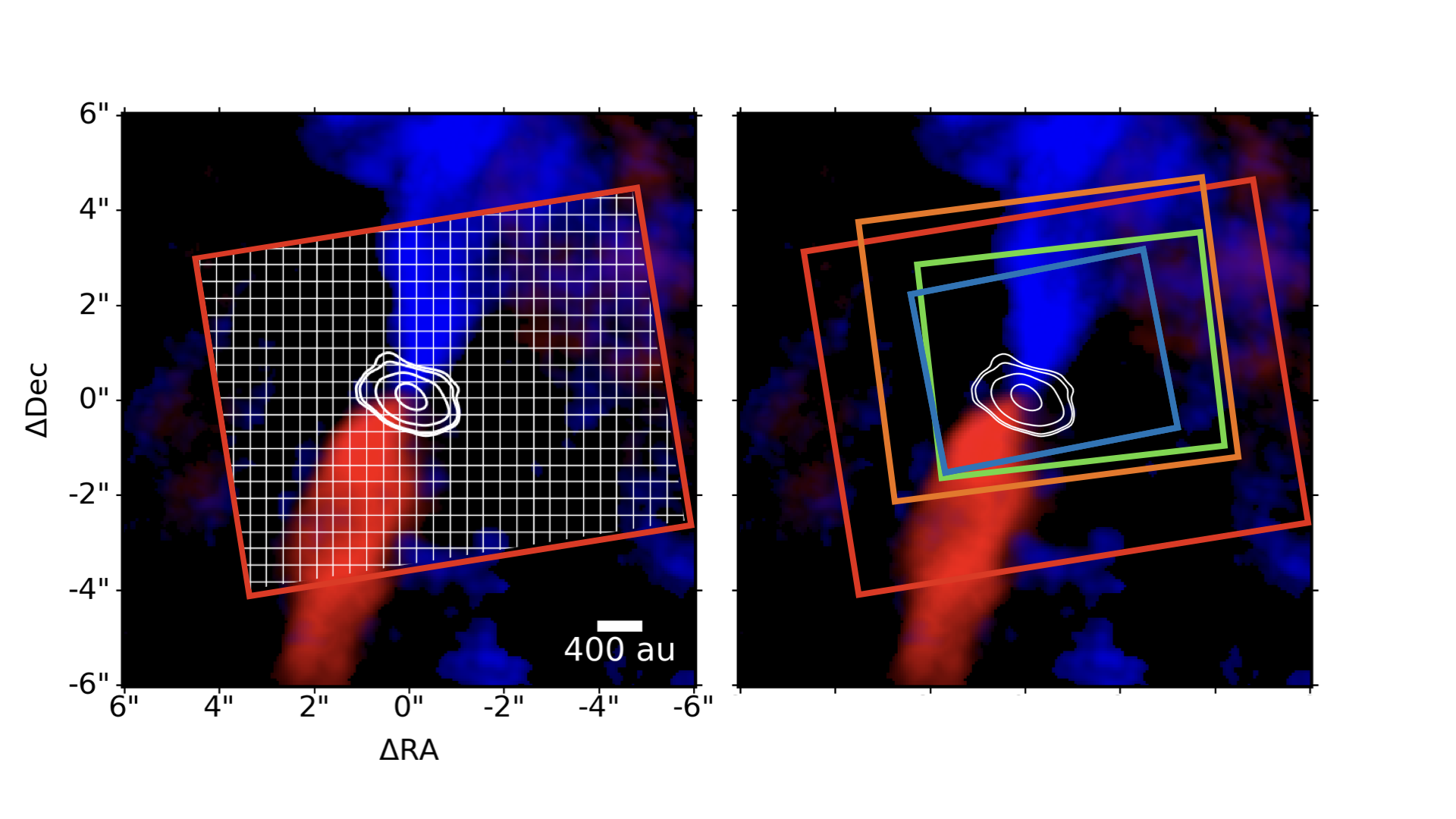
Figure 3: Right: MIRI-MRS IFU footprint for Channel 1 (blue), 2 (green), 3 (orange) and 4 (red) overlaid on the ALMA Serpens SMM3 CO 2–1 outflow map, using data from Tychoniec et al. (2021). Two dithers were used. The positions of the IFU have been chosen on purpose to be slightly offset toward the blue outflow lobe for the shortest wavelength channels, but still covering some part of the red outflow lobe. The white contours indicate the 1.3 millimeter continuum showing the dust disk. Left: illustration of the grid of individual spaxels for Channel 4.

The low-mass sample consists of nearby sources at distances $<$500 pc that cover both the deeply embedded Class 0 and more evolved Class I phases with bolometric luminosities ranging from 0.2 to $>$100 L_⊙ and bolometric temperatures from $<30$ K to 200 K (van Gelder et al., 2024a). They were furthermore selected to belong to only three star-forming regions – Perseus, Taurus and Serpens – to minimize slew overheads, with two pointings in the isolated BHR 71 cloud added. Some sources were chosen because they have prominent outflows and jets (e.g., L1448-mm, Ser-SMM1, BHR71). To further study outflow physics, two dedicated pointings at “knot” positions in the blue-shifted outflow lobes well offset from NGC 1333 IRAS4A and Ser-emb8(N) were added. The protostar position of NGC 1333 IRAS4A is covered in PID 1236 as part of JOYS+; hence this source is not further included in the analysis here. Moreover, the entire blue outflow lobe and a small portion of the red lobe of HH 211 were imaged with MIRI-MRS in program 1257. These three Class 0 sources (HH 211, NGC 1333 IRAS4A and Ser-emb8(N)) are so deeply embedded that they are not detectable even with JWST. Other sources were selected because of their very deep ice features facilitating the search for new minor ice species (e.g., B1-c). SVS4-5 is a special case because it is a “background” Class I/II source behind or inside the envelope of the Class 0 source Ser-SMM4 probing ices at very high densities (Pontoppidan et al., 2004; Perotti et al., 2020) and is not included in Table 1. A number of sources with confirmed young disks based on Keplerian rotation were included as well (e.g., L1527, TMC1, TMC1A).

Several sources are close binaries that can be resolved by MIRI at its shortest wavelengths, allowing comparison of their outflow and ice properties on scales of $<$1000 au. In total 17 low-mass sources (23 sources counting binaries individually) were targeted. Of these 17 (23) sources, 4 (6) are Class I and one source is borderline Class 0/I (L1527). Note that program 1236 (PI: M. Ressler) is focused on binary sources in Perseus so the comparison of binaries will be part of future JOYS+ publications.

For the high-mass sources, 3 Infrared Dark Clouds and 3 High-Mass Protostellar Objects (HMPOs) and hot molecular cores (HMCs) were chosen. Their properties and distances are included in Table 1. The MIRI-MRS data reveal several of these sources to be binaries or multiples: there are at least 9 mid-IR sources detected in the 6 high-mass MRS target fields: IRAS 23385+6053 (hereafter IRAS 23385) displays a binary (Beuther et al., 2023), G28 P1 two distant sources, IRAS 18089-1732 (hereafter IRAS 18089) at least three sources, and G28S shows no sources at 5 $\mu$m. G28 IRS2 and G31 show one source each. As for the low-mass sources, the high-mass set has been selected to cover a broad range of masses and evolutionary stages without saturating the MIRI-MRS. Note that many nearby well-known high-mass protostars studied with the ISO-SWS are too bright for JWST.

3.2 MIRI-IFU observations

The coordinates in Table 1 represent those of the protostellar source positions as found from millimeter interferometry. For the low-mass protostars, the actual MIRI-MRS IFU pointing positions are on purpose slightly offset from the millimeter continuum source position to cover a larger fraction of the less-extincted blue-shifted part of the outflow in the IFU, in addition to still catching some part of the red-shifted outflow. For TMC1A, the IFU has a larger offset from the source position to capture a larger fraction of its blue wind as imaged by ALMA (Bjerkeli et al., 2016). All MRS IFU pointing coordinates are summarized in Table 4. The mid-infrared peak positions of the low-mass sources derived from the MRS data are listed in Table B.1 of van Gelder et al. (2024a). A single NIRSpec IFU spectrum of the source B1-c with the G395M mode is taken as well within program 1290 to obtain a full inventory of this ice-rich source including HDO ice.

The sources within one cloud were observed in a single uninterrupted sequence with one background (dark) position observed in each cloud to characterize detector artifacts and subtract the telescope background. For Perseus, this background was taken to be the position of the millimeter source B1-bS which is so deeply embedded that it is undetected with JWST. For Taurus the background was taken with a single dither position whereas for the other three cases a 2-point dither was used.

All sources have been observed with the full MIRI-MRS spectral coverage using the three grating settings (A, B, C) to observe the 5–28 $\mu$m range spread over four Channels (1–4) of the MIRI IFU (Wells et al., 2015; Wright et al., 2023). A 2-point dither pattern for extended sources was adopted for most sources, except for B1-c and Ser-SMM1A for which a 4-point dither pattern was used. The typical integration time is 200 s per grating setting, except for L1527 which used 1000 s per grating and B1-c which had 2000 s in gratings A and C and 4000 s in grating B. This latter setting was chosen because grating B covers the deep silicate absorption around 10 $\mu$m where the source flux is much lower. The IFU field of view (FoV) varies between $3.2^{\prime\prime}\times 3.7^{\prime\prime}$ (Channel 1) and $6.6^{\prime\prime}\times 7.7^{\prime\prime}$ (Channel 4). Figure 3 illustrates the IFU footprint of the different channels for Serpens SMM3, covering the central object, its immediate envelope structure and the inner region of the blue outflow and jet.

For some sources, small mosaics ranging from 1$\times$2 to $3\times 3$ have been made of the blue outflow lobe mapping regions up to $12-20^{\prime\prime}$ in size. These observational details are provided in Table 4 in Appendix A; note that they are sometimes listed as separate pointings in the archive. The total extent of the HH 211 blue lobe and a small portion of its red-shifted one ($0.95^{\prime}\times 0.22^{\prime}$) has been observed with $12\times 2$ spatial settings (Caratti o Garatti et al., 2024). More details of the observations and mid-infrared continuum images of all low-mass sources in each of the four IFU channels are presented in Figures B.1-B.18 of van Gelder et al. (2024a) and in Caratti o Garatti et al. (2024) for HH 211.

Most of the JOYS sources were observed in Fall 2023. Only the high-mass source IRAS 23385+6053 (3000 L_⊙, 9 M_⊙) was observed early in the JWST mission, in August 2022. Hence most of the early JOYS analysis has focused on this source (Beuther et al., 2023; Gieser et al., 2023b; Francis et al., 2024). Located at a distance of 4.9 kpc in the direction of the outer Galaxy, this puts the source at a galactocentric radius of 11 kpc, making IRAS 23385 a unique laboratory for studying star formation in the outer Galaxy. This paper provides one of the first opportunities to look at similarities and differences among the larger JOYS sample from low to high mass.

3.3 MIRI-MRS data reduction

The MIRI-MRS data were reduced and calibrated using the JWST calibration pipeline version 1.13.4 (Bushouse et al., 2024) using reference context jwst$\_$1188.pmap. The steps adopted are the same as those in van Gelder et al. (2024a) of which only a short summary will be provided here. The raw data were processed through all three steps of the JWST calibration pipeline. This included the subtraction of the dedicated background on the detector level, where astronomical emission in the background was masked so that it was not subtracted in the science data. Furthermore, the fringe flat for extended sources (Crouzet et al., 2025) and the 2D residual fringe correction (Kavanagh et al. in prep.) were also applied on the detector level. Prior to building the cubes, an additional bad pixel map was created using the Vortex Imaging Package (VIP) version 4.1 (Christiaens et al., 2023). Last, the final data cubes were constructed for each channel and subband separately with the outlier rejection and master background steps switched off. Spectra were extracted manually from selected positions in the datacubes using either an aperture with a constant diameter as function of wavelength (“circle”) or an aperture with its diameter increasing with wavelength (“cone”) following the size of the point spread function (PSF; Law et al., 2023).

Table C.1 of van Gelder et al. (2024a) provides 1$\sigma$ noise level estimates in each of the MRS sub-bands for the JOYS low-mass targets at the continuum source position(s). They typically range from 0.1 mJy in Channels 1–3 to several mJy in Channel 4, with some sources (e.g., B1-a-NS and TMC1A) having higher noise levels due to their strong continuum or being located at the edge of the FoV. Noise levels are similar for the high-mass sources because of their similar integration times.

3.4 Simultaneous imaging

During the MIRI-MRS observations, the imager was turned on to simultaneously observe a field of $74^{\prime\prime}\times 113^{\prime\prime}$ offset by $\sim 1^{\prime}$ from the MRS position at a position angle determined by the time of observations. This simultaneous imaging provides not only serendipitous science such as finding new deeply embedded protostars in the cloud, but it also serves as the absolute astrometric calibration of the MRS data by comparing with the positions of field stars that are in the Gaia catalog. Indeed, for the initial JOYS source IRAS 23385+6053, for which the source position was well known, an adjustment of 1.61^′′ in RA and 0.35^′′ in Dec in the telescope coordinates was needed based on comparison with the Gaia stars.

The imager has a plate scale of 0.11^′′ (Bouchet et al., 2015) and provides diffraction-limited imaging in a number of broadband filters. For the JOYS program, simultaneous imaging was obtained in the F1500W broadband filter centered at 15.0 $\mu$m (FWHM 2.92 $\mu$m) (Beuther et al., 2023). At that wavelength, the MIRI PSF is 0.49^′′ FWHM, providing nearly an order of magnitude sharper images than was possible with previous space instruments. The 15 $\mu$m filter was chosen to be away from PAH features, and to be intermediate between the Spitzer IRAS 8 $\mu$m and MIPS 24 $\mu$m bands to fill in that part of the SED. Being at a wavelength where the telescope background does not yet contribute, it also provides a good compromise between high angular resolution and good sensitivity at the longer MIRI wavelengths that can probe most deeply into the clouds. Note that this filter is centered at the CO₂ ice band, however, which can absorb a significant fraction of the protostellar continuum along the line of sight through the envelope.

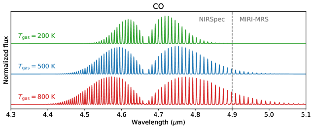
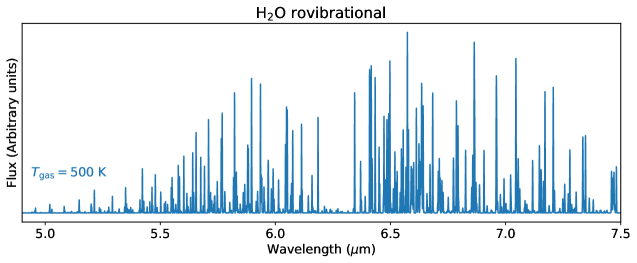
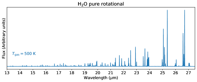
Figure 4: Examples of normalized mid-infrared slab model molecular emission spectra in the optically thin regime. From top to bottom: CO at 500 K compared with 200 and 800 K; H₂O ro-vibrational lines at 5–7 $\mu$m; H₂O pure rotational lines at 13–28 $\mu$m.

The MIRI images were processed through all three steps of the JWST calibration pipeline using reference context jwst$\_$1235.pmap adopting the default parameters in each step. In the final step, the tweakreg step was switched off since very few Gaia stars are available in the FoV. The background level was estimated and subtracted by setting the skymethod option to local in the skymatch step. An example of the science that can be done with these simultaneous images to find new protostars in the outer Galaxy is provided in Appendix C.

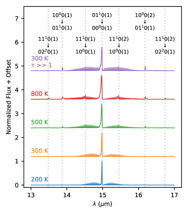
Figure 5: Simulated normalized CO₂ mid-infrared spectra at different temperatures for optically thin emission (blue to red). Note the broadening of the $Q$ branch and the appearance of hot bands (i.e., transitions between vibrationally excited states) with increasing temperature. These hot bands also become visible at lower temperatures when the CO₂ $Q-$branch emission becomes optically thick (purple).

3.5 Analysis of gas-phase spectra

The analysis of atomic lines and ices seen in the MIRI spectra is described in the various scientific sections. Here we summarize the analysis of gas-phase molecular lines to infer column densities and temperatures, following Francis et al. (2024); van Gelder et al. (2024a); Salyk et al. (2024) and papers studying molecular emission lines from disks (e.g., Salyk et al., 2011; Banzatti et al., 2025; Temmink et al., 2024a, and refs cited).

In the simplest case of spectrally resolved pure absorption and assuming an isothermal slab model, the measured optical depths are directly related to column densities. For unresolved lines such as with JWST, an intrinsic line width needs to be assumed and a curve-of-growth type of analysis to be performed (Boonman et al., 2003a; Barr et al., 2020); typical values are a FWHM of a few km s^-1 up to 10–20 km s^-1 (van Gelder et al., 2024a; McClure et al., 2025). It is usually assumed that the covering fraction of the absorbers against the continuum is unity and that the gas is at a single temperature, but this does not need to be the case (Knez et al., 2009; Li et al., 2024). Proper radiative transfer may therefore be needed (González-Alfonso et al., 2002; Lacy, 2013).

Mid-infrared emission lines are also usually interpreted with isothermal slab models fitted to continuum-subtracted spectra. The emission is assumed to originate in a plane-parallel cylindrical slab of radius $R$ and column density $N$. The radius $R$ should not be viewed as a disk or envelope radius but rather represents the emitting area $\pi R^{2}$ having any shape at any location in the beam. The gas is taken to be at a single excitation temperature $T_{\rm ex}$, and Figure 4 shows typical ro-vibrational spectra of CO and H₂O at 200–800 K. Note that MIRI only probes the tail of the CO $v$=1-0 $P$ branch at high temperatures, and that the 5–28 $\mu$m range covers both the H₂O ro-vibrational bending mode lines as well as a forest of pure rotational water lines. Figure 5 illustrates how the CO₂ spectrum changes with temperature and optical depth (see also Cami et al., 2000; Bosman et al., 2017). Emission lines can be strongly affected by extinction from ices and dust, see § 6 and Appendix G for details.

If collisions dominate the excitation, $T_{\rm ex}$ will approach the kinetic gas temperature $T_{\rm kin}$, but the critical densities for this assumption to be valid are high, typically $>10^{12}$ cm^-3 for vibrational lines (e.g., Bruderer et al., 2015). Such high densities may only be achieved in the inner few au of disks (Salyk et al., 2009; Carr & Najita, 2011). Non-LTE effects will be important for regions with lower densities such as in shocks or in hot cores, where densities are typically $10^{6}$ to $10^{8}$ cm^-3 on scales of 50 au (Kristensen et al., 2012; Notsu et al., 2021). However, in this case strong infrared radiative pumping through ro-vibrational transitions, by a radiation field whose intensity at the pumping wavelengths can be characterized by a temperature $T_{\rm rad}$, can boost the vibrational emission (see e.g., Bruderer et al., 2015; van Gelder et al., 2024b, for the cases of HCN and SO₂).

In contrast, the rotational distribution within the $v=0$ vibrational ground state can be thermalized by collisions at lower densities, and this rotational distribution, characterized by $T_{\rm rot}$, is largely conserved in the vibrationally excited states through infrared pumping and can thus reflect the kinetic temperature $T_{\rm kin}$. For molecules with a dipole moment, the density to achieve $T_{\rm rot}$ close to $T_{\rm kin}$ is around $10^{8}-10^{9}$ cm^-3, whereas the rotational level populations of molecules without a dipole moment such as CO₂ are thermalized at much lower densities. In other words, $T_{\rm vib}$ is usually larger than $T_{\rm rot}$, with the former being controlled by radiative pumping at $T_{\rm rad}$ and the latter being closer to the gas temperature $T_{\rm kin}$.

4 Onset of star formation: protostars and accretion

4.1 Probing the fossil accretion record from imaging

JWST’s ability to probe the deeply embedded Class 0 stage is illustrated by the HH 211 outflow ($d$=321 pc, Ortiz-León et al. 2018b). Despite the extent and power of this outflow, as highighted by prominent shocked atomic, H₂ and CO emission at infrared and millimeter wavelengths (e.g., McCaughrean et al., 1994; Gueth & Guilloteau, 1999; Lee et al., 2009; Dionatos et al., 2018), the current stellar mass as determined from kinematic studies is still comparable to that of a brown dwarf, only 0.08 M_⊙ (Lee, 2015).

JWST-NIRCam infrared imaging of HH 211, taken as part of JOYS, has revealed its jet and outflow structure with unprecedented detail in both molecular (H₂, CO) and atomic ([Fe II]) lines (Ray et al., 2023). Because of its youth, the outflow is still compact and can readily be imaged in its entirety with JWST. The NIRCam images reveal an abundance of H₂ knots in the innermost highly-extincted collimated jet which were previously undetected and/or unresolved (see Figure 6). Note that the central source of HH 211, i.e., the protostar itself, remains undetected even with JWST’s sensitivity, hidden behind $A_{V}>$100 mag of extinction.

These H₂ knots provide a fossil record of the recent accretion history of the protostar. Comparison with archival VLT-ISAAC K-band images taken 20 years earlier demonstrates JWST’s capabilities to measure the proper motions and thus the 3D kinematics of the outflow of this very young protostar (Ray et al., 2023). The tangential flow velocity has been measured to be $\sim$100 km s^-1 so the timescale to cross the entire length of the blue outflow lobe (1${}^{\prime}\sim$ 18300 au at 321 pc) is only $\sim$1000 years. Here we use the data from Ray et al. (2023) to show in Figure 6 that the spacing and structure of the jet knots is as short as $\sim$ 5 yr. Taken together, this seems to imply that this protostar has built up its current mass of 0.08 M_⊙ over a period of $\sim$1000 yr in multiple bursts every 5–10 yr, and is still growing in mass.

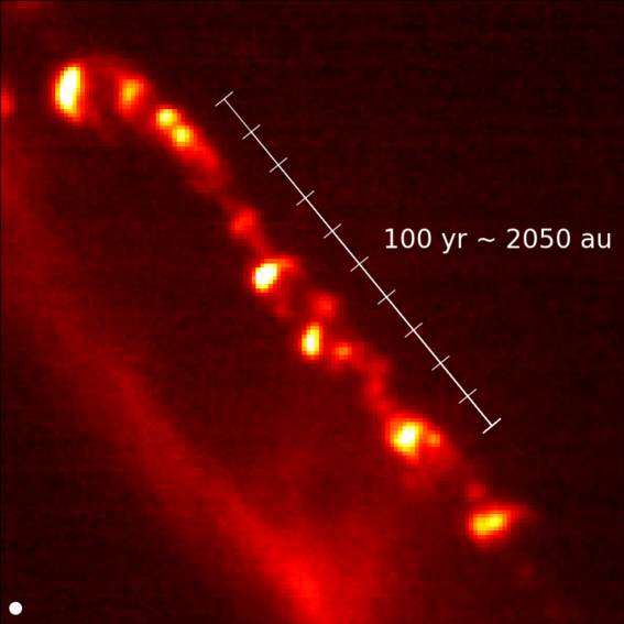
Figure 6: Blow-up of the H₂ knots in part of the HH 211 jet in the blue outflow lobe imaged with the NIRCam F212N filter (Ray et al., 2023). This figure illustrates the typical separation between knots, and thus implicitly the timescales between accretion bursts. The ruler shows the distance of jet gas covered in 100 yr when traveling at 100 km s^-1, in 10 sections of 10 yr each.

4.2 H I recombination lines as accretion tracer

High mass protostars.

MIRI’s potential to measure accretion rates for high-mass protostars has been provided by the analysis of IRAS 23385+6053 ($d$=4.9 kpc, Table 1) (Beuther et al., 2023; Gieser et al., 2023b), a region forming a 9 M_⊙ high-mass protostar (Cesaroni et al., 2019). The high spatial resolution of MIRI reveals that this source is actually a binary system (labelled A and B) with a projected linear separation of $\sim$3300 au that can be resolved in the MRS short wavelength channels. Only the A source coincides with the extension of the millimeter continuum peak. The H I 7-6 Humphreys $\alpha$ line is detected at a 3-4$\sigma$ level toward sources A+B. Follow up analyses reveal that most of the ionization comes from source A (Reyes et al., in prep.). Using the Rigliaco et al. (2015) relation for this line calibrated for low-mass T Tauri stars, an accretion luminosity of 140 L_⊙ can be inferred, which in turn gives an accretion rate of $2.6\times 10^{-6}$ M_⊙ yr^-1. Correcting this number for an estimated visual extinction of 30–40 mag based on the depth of the silicate feature and using the McClure (2009) extinction law, increases the rate to $\sim 10^{-4}$ M_⊙ yr^-1. For such a high extinction, the bulk of the A+B sources’ luminosity of $3\times 10^{3}$ L_⊙ is indeed due to accretion. An analysis of H I in the full JOYS high-mass sample will be presented in Reyes et al. (in prep.).

Table 2: Hydrogen line measurements and accretion rates

Source	$A_{V}$	$L_{\rm bol}$	$M_{\star}$	$R_{\star}$	$L_{\rm acc}/L_{\rm bol}$	Flux H I 7-6	$L_{\rm acc}$	$\dot{M}_{\rm acc}$	$\dot{M}_{\rm acc}$
							from H I 7-6	from H I 7-6	from $L_{\rm bol}$
	(mag)	(L⊙)	(M⊙)	(R⊙)		(erg cm-2 s-1)	(L⊙)	(M⊙ yr-1)	(M⊙ yr-1)
[5pt] TMC1-W	18	0.35	0.20	2.5	0.5	$4.0\pm 1.1\times 10^{-15}$	$1.2\times 10^{-2}$	$4.9\times 10^{-9}$	$7.2\times 10^{-8}$
TMC1A	33	2.70	0.56	2.5	0.5	$6.8\pm 2.7\times 10^{-14}$	$4.5\times 10^{0}$	$6.6\times 10^{-7}$	$2.0\times 10^{-7}$
SerpSMM3	50	27.5	0.50	4.0	1.0	$<5.4\times 10^{-16}$	$<2.0\times 10^{-2}$	$<5.2\times 10^{-9}$	$7.2\times 10^{-6}$

Low-mass protostars.

An early JOYS example for low-mass protostars is provided by TMC1, a Class I binary located in Taurus at 142 pc distance (Tychoniec et al., 2024). Several H I recombination lines are detected toward both sources, with the strongest lines seen toward TMC1-W. The fact that these lines are only seen on top of the IR continuum, i.e., at the source position, suggests that there is no or little jet contribution. Table 2 lists the inferred accretion rate, using the relation by Rigliaco et al. (2015) and correcting for extinction and contamination by water lines (see below and update by Tychoniec 2025). The value of $5\times 10^{-9}$ M_⊙ yr^-1 is an order of magnitude lower than that derived from the bolometric luminosity $L_{\rm bol}$ also listed in Table 2 obtained assuming the relation ${\dot{M}}_{\rm acc}=fR_{*}L_{\rm bol}/GM_{*}$ holds. Here $f=L_{\rm acc}/L_{\rm bol}$ is the fraction of the luminosity that is ascribed to accretion. The low value found for TMC1-W suggests that it is currently in a low accretion state, perhaps similar to the low-mass Class 0 source IRAS 16253-2429 studied with JWST in the IPA program (Narang et al., 2024).

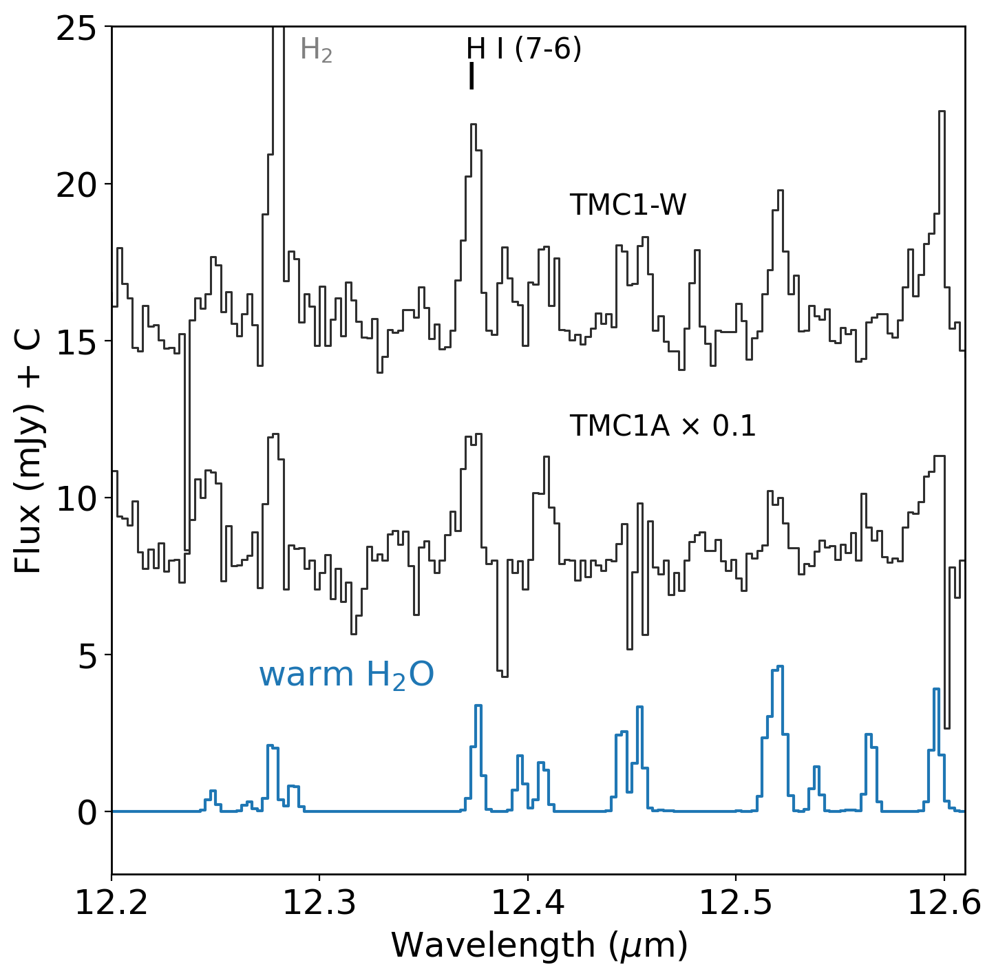
Figure 7: The H I 7-6 Humphreys $\alpha$ line detected in the JWST-MIRI spectrum of the Class I source TMC1A compared with that seen toward TMC1-W (Tychoniec et al., 2024). For comparison, also a warm water spectrum at $T$=485 K is shown (best fit for TMC1-W, van Gelder et al. 2024a), to illustrate that water emission can contribute to the H I 7-6 feature.

Another well-studied nearby Class I source in Taurus within the JOYS sample is TMC1A (IRAS 04365+2535). This $\sim$0.5 M_⊙ protostar has a striking blue-sided molecular disk wind imaged with ALMA (Bjerkeli et al., 2016) and has recently been studied with JWST-NIRSpec by Harsono et al. (2023) revealing a collimated jet in [Fe II] 1.644 $\mu$m. Using the NIRSpec Pa$\beta$ and Br$\gamma$ lines and assuming that all the luminosity comes from protostellar accretion, very low rates of $2\times 10^{-12}$ and $3\times 10^{-9}$ M_⊙ yr^-1 have been reported (Harsono et al., 2023). Note that neither value is corrected for extinction, which may also be responsible for the differences between the two diagnostics.

We can revisit the TMC1A case with our MIRI data since the 7-6 Humphreys $\alpha$ line at 12.37 $\mu$m is detected and suffers much less from extinction (Fig. 7). Moreover, the extinction can be estimated, albeit with considerable uncertainty, to be $A_{V}\approx 30$ mag from the silicate optical depth using $A_{V}=18.5\times\tau_{\rm 9.7}$. Using the same relation of Rigliaco et al. (2015) and correcting for extinction and water, a mass accretion rate of $6.6\times 10^{-7}$ M_⊙ yr^-1 is found for TMC1A. This value is much higher than inferred from the uncorrected NIRSpec data and consistent with those estimated from the bolometric luminosity of the source and the need to build up a $\sim$1 M_⊙ star in less than 1 Myr. It agrees well with accretion rates found by Fiorellino et al. (2023) for a large sample of much less extincted Class I sources based on Br$\gamma$ data. The case of SMM3 is discussed below in § 5.1. Note that all accretion rate determinations depend strongly on the assumed extinction toward the protostellar embryo; a detailed discussion of the different extinction diagnostics is presented in Appendix G.

Note that the H I 7-6 line at 12.372 $\mu$m used to determine these accretion rates is actually located near another recombination line, the H I 11-8 transition at 12.387 $\mu$m. The Spitzer-IRS could not resolve these lines, but MIRI-MRS can (Franceschi et al., 2024); the empirical relation of Rigliaco et al. (2015) is therefore taken to refer to the sum of both components. Also, as Figure 7 shows, the H I flux can be contaminated by warm water emission. However, the fluxes of TMC1-W and TMC1A cannot be fully explained by water: H I still dominates the 12.37 $\mu$m emission. Any water contribution can be subtracted using a fit to the H₂O emission over a larger wavelength range, as has been done for the values listed in Table 2 (Rigliaco et al., 2015; van Gelder et al., 2024a). An updated water-corrected relation is presented in a recent JWST-based study by Tofflemire et al. (2025), which gives consistent results for our sources.

Another complication is that not all H I recombination line emission need to originate from accretion onto the protostars and that scattering can complicate the extinction correction at shorter wavelengths (Delabrosse et al., 2024). Brackett $\alpha$ NIRSpec imaging shows bright extended emission in some sources that is clearly associated with shocks in protostellar jets (Federman et al., 2024; Neufeld et al., 2024). VLTI-Gravity observations that resolve the Brackett $\gamma$ emission in Class I/II T Tauri systems also demonstrate that winds and outflows commonly contribute to the H I emission at the scale of the inner disk (Gravity Collaboration et al., 2023). Also, the Rigliaco et al. (2015) relation was derived from Spitzer data in large apertures that could have included extended H I emission, thereby assigning all the H I to accretion rather than a mix of accretion and ejection. Thus, the inferred accretion rates from H I should be considered as upper limits. A combination of spatially and spectrally resolved H I lines observable with MIRI and NIRSpec tracing a range of temperatures and densities, combined with H I excitation calculations (Kwan & Fischer, 2011), is needed to disentangle the components.

5 Protostellar jets, winds and outflows

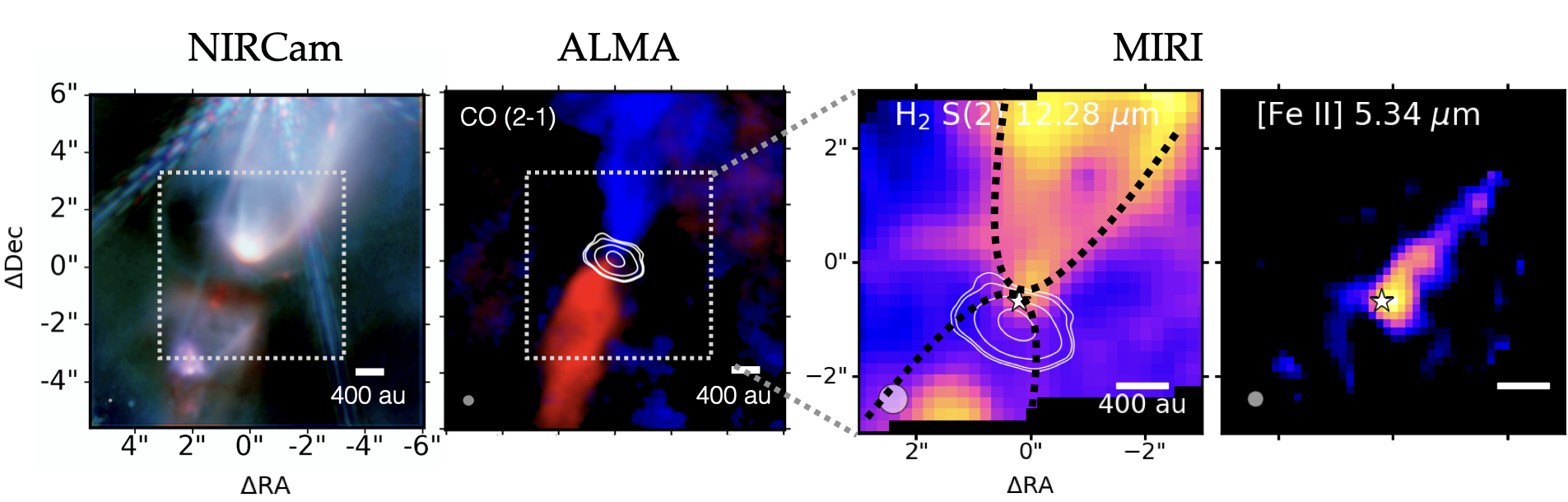
Figure 8: Comparison of JWST and ALMA data for the Class 0 protostar Serpens SMM3. From left to right: (1) JWST NIRCam image of SMM3 using a combination of the F210M (blue), F360M (green), and F480M (red) filters from archival data of PID 1611; (2) ALMA image of the CO $J$=2–1 red and blue outflow lobes in the inner $10"\times 10"$, together with the dust disk at 1.3 millimeter continuum emission (contours) (Tychoniec et al., 2021); (3) JOYS MIRI-MRS maps of the H₂ S(2) line at 12.28 $\mu$m, with the dotted line outlining the scattered light cavity seen with NIRCam; and (4) the [Fe II] line 5.34 $\mu$m, both in a zoomed-in region of $6"\times 6"$. Beam sizes are indicated in the lower left corner of each panel.

MIRI-MRS jet, wind and outflow studies have been published within JOYS for the high-mass protobinary IRAS 23385+6053 (Beuther et al., 2023; Gieser et al., 2023b) and for the low-mass protobinary system TMC1 (Tychoniec et al., 2024). Moreover, the entire blue outflow lobe and part of the red lobe of HH 211, $1^{\prime}$ in extent, has been mapped with the MRS (Caratti o Garatti et al., 2024). The latter study thus includes also the bow shocks at the tip of the outflow, in addition to the jets and winds closer to the protostar. See Fig. 1, § 2 and Appendix B.2 for the definition of these terms as used in this paper and for scientific background.

5.1 The Class 0 source Serpens SMM3 as an example

Here we present the case of the Class 0 source Serpens SMM3 ($d$=439 pc, Table 1) to illustrate typical findings in MRS maps. SMM3 is, with 28 L_⊙, among the most luminous of the low-mass sources in the JOYS sample. It has been imaged by ALMA in various molecular lines (Tychoniec et al., 2021, and refs cited) and has a relatively narrow CO outflow opening angle of $<20^{o}$. It is one of the few Class 0 sources with clear “knots” seen in CO and SiO about 8^′′ offset from the source along the jet (also called extremely high velocity (EHV) “bullets”). It also shows hints of a large embedded rotating disk, further discussed in § 8. Finally, NIRSpec IFU data exist as part of JOYS+ (PID 1186) that can enhance the analysis in future studies, especially by observing more accretion tracers and ro-vibrational H₂ and CO lines (Le Gouellec et al., 2024b).

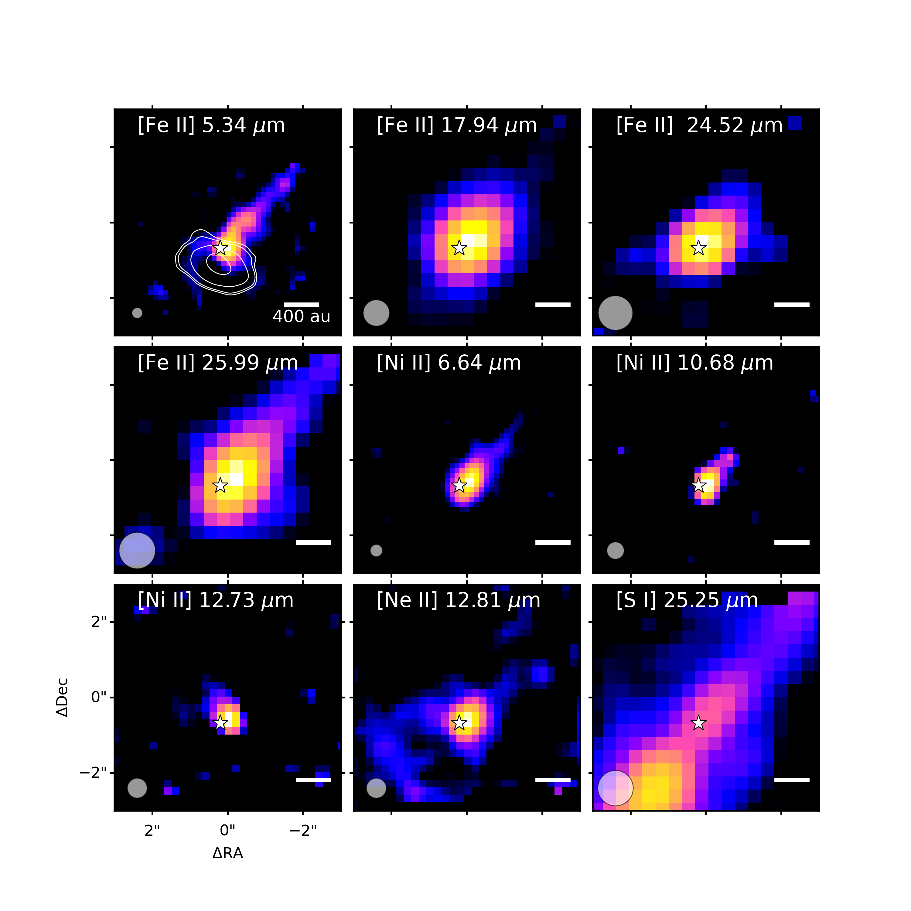
Figure 9: MIRI-MRS maps of various atoms and ions toward the Class 0 protostar Serpens SMM3. The white contours in the top left panel outline the dust disk seen in millimeter continuum. Beam sizes are indicated in the lower left corner of each panel. Each panel is scaled to the maximum emission of that species. The maximum and minimum colors are (in Jy km s^-1), from top left to bottom right: [Fe II] 5.34 (0.033, 0.003); [Fe II] 17.94 (0.84, 0.017); [Fe II] 24.52 (0.62, 0.025); [Fe II] 25.99 (1.86, 0.075); [Ni II] 6.64 (0.05, 0.002); [Ni II] 10.68 (0.006, 0.001); [Ni II] 12.73 (0.005, 0.001); [Ne II] 12.81 (0.017, 0.003); [S I] 25.25 (3.27, 0.033).

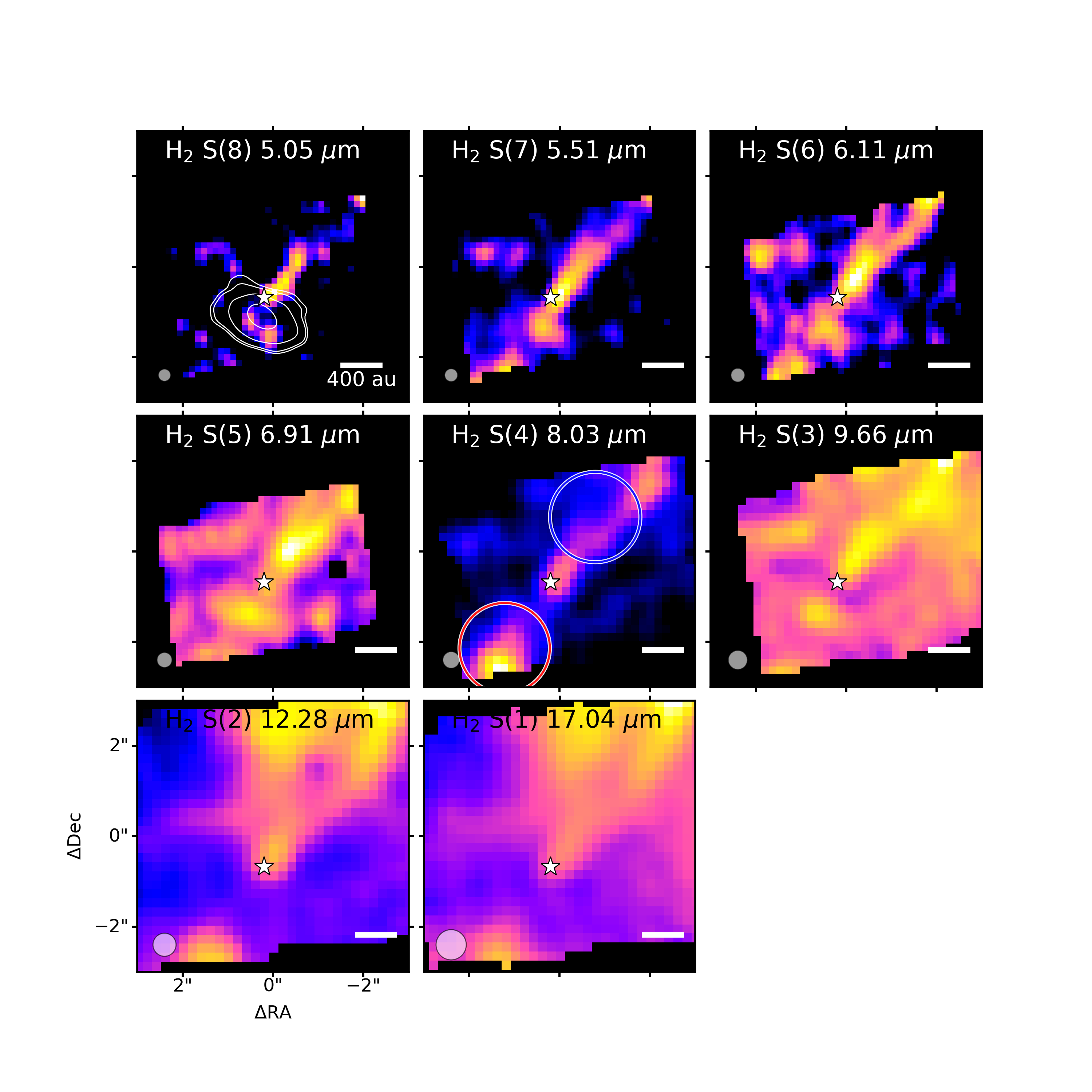
Figure 10: MIRI-MRS maps of the various H₂ lines toward the Class 0 protostar Serpens SMM3. The white contours in the top left panel indicate the dust disk seen in millimeter continuum. The red and blue circles on the S(4) image indicate the positions where the H₂ spectra and rotational diagrams have been extracted. Note that the S(3) image at 9.66 $\mu$m is strongly affected by silicate extinction, and the S(5) line at 6.9 $\mu$m by ice extinction, hence their maps are more noisy. Beam sizes are indicated in the lower left corner of each panel. Each panel is scaled to the maximum emission of that species. The maximum and minimum colors are (in Jy km s^-1), from top left to bottom right: S(8) (0.008, 0.003); S(7) (0.033, 0.007); S(6) (0.013, 0.003); S(5) (0.026, 0.003); S(4) (0.089, 0.009); S(3) (0.035, 0.005); S(2) (0.090, 0.009); S(1) (0.084, 0.008).

MRS maps.

Figure 8 (left) presents a NIRCam image of SMM3 over the inner $10"\times 10"$ region together with an ALMA image showing the swept-up CO outflow as well as the SMM3 dust disk in millimeter continuum. The two right-hand panels highlight the inner $6"\times 6"$ in the H₂ S(2) line at 12.28 $\mu$m and the [Fe II] line 5.34 $\mu$m. Only a single MRS pointing was obtained for this source, thus covering only part of the outflow. The [Fe II] image clearly reveals the collimated jet, whereas the H₂ line shows the wider-angle warm molecular gas inside the outflow cavity outlined by the NIRCam scattered light image. Mid-IR emission is stronger in the blue lobe than in the red lobe due to enhanced extinction in the latter close to the source (see also below).

MIRI images of various other atomic lines and of H₂ covered in the MRS data are presented in Figures 9 and 10. Note that the spatial resolution decreases with wavelength from $\sim 0.2^{\prime\prime}$ at 5 $\mu$m to $\sim 0.7^{\prime\prime}$ at 25 $\mu$m. All four [Fe II] lines trace the blue part of the jet, even at the longest wavelength of 25.99 $\mu$m, but interestingly, the [S I] 25.25 $\mu$m line, which is close in wavelength, shows a more prominent peak on the red side of the outflow. This demonstrates that the lack of [Fe II] emission on the red side is real, and not just due to extinction; it could be due to lower excitation and shock conditions along the red-shifted jet. The intensity of all four [Fe II] lines is sensitive to density and shock velocity, although to different degrees (Hartigan et al., 1987; Hollenbach & McKee, 1989). In particular, the [Fe II] 25.99 $\mu$m line is a fine-structure transition within the ground electronic state with the lowest critical density, similar to that of the observed [S I] 25.2 $\mu$m, yet this [Fe II] line is also not detected. This suggests that in addition to excitation, abundance differences also play a role: less Fe may have been returned to the gas phase on the red side by the shocks.

The [Ni II] and [Ne II] lines peak close to the source in the blue part of the jet (Fig. 9). For [Ni II] its limited extent in SMM3 may be due to its lower $S/N$, since in other still-unpublished JOYS sources it usually follows [Fe II]. In contrast, [Ne II] often shows more central emission, although it has a weak jet component as well for SMM3.

Figure 10 presents images of the various H₂ lines covered by the MIRI-MRS. Whereas the low-lying S(1) and S(2) lines trace the wide angle wind, the images of the higher H₂ lines are much narrower and clearly trace the jet, as seen most prominently in the H₂ S(7) and S(8) lines at the shortest MIRI wavelengths of 5.51 and 5.05 $\mu$m where the images are sharpest and comparable in resolution to those of the [Fe II] 5.34 $\mu$m. Moreover, as also seen in Fig. 8, H₂ is clearly detected in the red outflow lobe as well, even at 5.5 $\mu$m. In fact, the H₂ S(4) line reveals two new “knots” on opposite sides of the source. Interesting, there appears to be a slight tilt between the warm H₂ low-$J$ images and that of the hot H₂ and atomic lines. No HD is detected at either position, consistent with the fact that the H₂ lines in SMM3 are not as bright as those in HH 211 where several HD lines are seen (Francis et al., 2025, see also Appendix B). Figure 11 presents the moment-1 map of the H₂ S(1) and [S I] 25 $\mu$m lines, clearly separating the red and blue parts in [S I]. Radial velocities of $\sim$20 km s^-1 are seen for H₂ and [S I].

Taken together, these data suggest that – like for HH 211 – the SMM3 jet has a “nested” structure with an ionized core surrounded by a molecular layer. This ionized core, however, appears on just one side of the outflow. Evidence for a wide-angle wind is found as well in low-$J$ H₂ lines. This example also shows that the full suite of atomic, ionic and molecular lines is needed to reveal the physical and chemical structure of the outflow.

H₂ excitation and extinction determination.

H₂ line fluxes have been extracted near two “knot” positions in a $\sim$1^′′ aperture and put in a rotational diagram. The results for the blue and red positions are presented in Figure 12. As has been commonly found, also from ISO and Spitzer data (e.g., van Dishoeck, 2004; Neufeld et al., 2006; Maret et al., 2009; Giannini et al., 2011; Gieser et al., 2023b), the upper level column densities derived from the S(3) line clearly fall below the trend of the other lines due to additional extinction by the silicate feature in the envelope. This deficit can therefore be used to infer the overall extinction in combination with an assumed overall extinction curve. Here the KP5 extinction curve of Pontoppidan et al. (2024a) has been used which has a somewhat stronger silicate feature than the McClure (2009) extinction curve.

At least two temperature components are needed to fit the remainder of the H₂ lines, consistent with previous findings (see above references). Using a procedure to obtain a simultaneous best fit for the two temperatures plus ortho-to-para ratio (OPR) and extinction results in the values indicated in the panels (Francis et al., 2025). The warm temperature is typically $\sim$600 K, whereas the hot temperature is $\sim$2000-3000 K. The OPR ratio is 2.0–2.5, close to the high temperature value of 3. Interestingly, the extinction is found to be only slightly higher for the red lobe, $A_{V}\approx 25$ mag, versus 15 mag for the blue lobe (Fig. 12).

The temperature structure as derived from H₂ can vary along the outflow axis, but also across it. Indeed, the fact that the low-$J$ H₂ lines have a wider opening angle than the high-$J$ lines indicates that gas temperatures decrease away from the jet axis (Tychoniec et al., 2024; Caratti o Garatti et al., 2024; Delabrosse et al., 2024). For the case of Serpens SMM3, the temperature of the warm component decreases by about 100–150 K from 600 K in an aperture centered close to the outflow cavity wall. Ultimately, mapping of the temperature structure of the wind may put constraints on the heating mechanisms and thereby also its launching mechanisms.

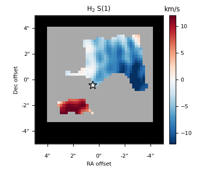
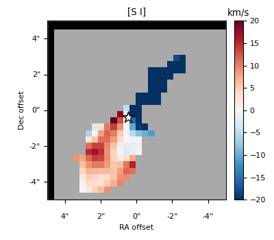
Figure 11: MIRI-MRS moment-1 maps of the H₂ S(1) 17.0 $\mu$m and [S I] 25.25 $\mu$m lines toward Serpens SMM3, showing the MRS’s ability to distinguish the red- and blue-shifted gas. The velocities are relative to the source velocity of $V_{\rm LSR}=7.6$ km s^-1.

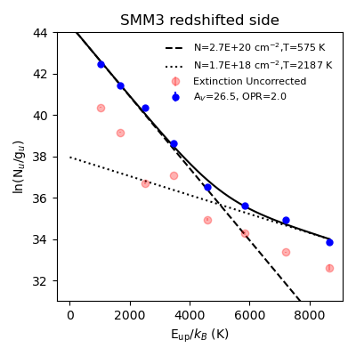
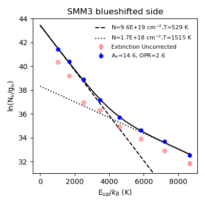
Figure 12: Rotational diagrams of H₂ at the blue (left) and red (right) lobes using spectra extracted at the positions indicated in Fig. 10. The light red points indicate the values before extinction correction, the full blue points after extinction correction. Two temperatures and an ortho-to-para ratio (OPR) have been fitted to the extinction-corrected fluxes.

Mass loss rates.

The H₂ column densities found from the rotational diagrams can be used to calculate mass loss rates through

$${\dot{M}}_{\rm H_{2}}=2\mu m_{\rm H}({\overline{N}}A)(v_{\rm tg}l_{\rm tg})$$ (1)

where ${\overline{N}}$ is the warm H₂ column density averaged over the emission area $A$ (assumed to be circular and equal to the area over which the spectrum has been extracted, Fig. 10 and 12), $v_{tg}$ is the tangential velocity and $l_{\rm tg}$ is the projected knot size. The width of the blue-shifted knot $l_{\rm tg}$ is measured to be 625 au at the position of the extracted spectrum from the lowest $J$ lines, whereas the line-of-sight velocity is –18 km s^-1 based on the average of the velocity shifts from the H₂ S(1) to S(4) lines that best trace the warm component (Fig. 11). Assuming an inclination of 50^o estimated from CO millimeter maps (Yıldız et al., 2015) and taking the extinction corrected warm H₂ column of $9.6\times 10^{19}$ cm^-2 derived from the rotation diagram (Fig. 10), gives a mass loss rate from the warm H₂ component of ${\dot{M}}_{\rm H_{2}}=1.4\times 10^{-7}$ M_⊙ yr^-1 with a factor of $\sim$2 uncertainty due to uncertainties in inclination and extinction. This value is a factor of a few lower than the mass loss rate of $7\times 10^{-7}$ M_⊙ yr^-1 found for HH 211 from warm H₂.

The advantage of using H₂ is that the total column of hydrogen nuclei is measured directly, as is its velocity, so no density or velocity needs to be inferred indirectly from diagnostics and models. Mass loss rates can also be derived from the atomic lines, as shown in detail for the case of HH 211 by Caratti o Garatti et al. (2024). Appendix D describes slightly different methods used here to estimate ejection rates from the extinction-corrected [Fe II] 26 $\mu$m line (Watson et al., 2016), the [Ne II]+[S I] lines combined with shock models from Hollenbach & McKee (1989) (Tychoniec et al., in prep.) and from the [O I] 63 $\mu$m line (Hollenbach, 1985).

These atomic diagnostics give values of $\dot{M}_{\rm jet}$ that are slightly lower than derived from H₂ by a factor of 2–3 when applied to one outflow lobe (Appendix D). Taking into account the factor of $\sim$3 higher velocities of the atomic component compared with H₂, the atomic and molecular jets seem to provide comparable thrust (momentum flux) $\dot{M}\times v_{\rm tot}$ to drive the material in the SMM3 system; the molecular component is not as dominant here as it has been found to be for HH 211 (Caratti o Garatti et al., 2024).

When summed over the entire MRS Channel 4 $7"\times 7"$ FOV, the [Fe II] 26 $\mu$m mass loss rate is $\dot{M}_{\rm jet}$ = 4.0 $\times 10^{-7}$ M_⊙ yr^-1. This value is within a factor of two of that based on the Herschel-PACS [O I] 63 $\mu$m luminosity in a $\sim 9"$ spaxel (Mottram et al., 2017). Note that the [Fe II] 26 $\mu$m relation of Watson et al. (2016) has been calibrated against [O I] 63 $\mu$m for a large sample of sources and that in general the [O I] value should be considered as an upper limit (see Appendix D).

How do these mass outflow values compare with the mass accretion rate? No hydrogen recombination lines are detected for SMM3 but the upper limit on the H I 7–6 line is not very constraining, assuming an extinction of 50 mag (see Table 2). This is likely caused by H I being obscured by the big and massive disk of SMM3, making it more difficult to peer in deeply close to the star. A rough estimate can be obtained assuming that the observed bolometric luminosity is mainly due to accretion for Class 0 sources like SMM3. Using the relation given in § 4, Mottram et al. (2017) find a value of $1.2\times 10^{-5}$ M_⊙ yr^-1. Thus, ${\dot{M}}_{\rm jet}/{\dot{M}}_{\rm accretion}\approx$0.01. This value is on the low side of previous determinations for other Class 0 and I sources (Watson et al., 2016). Since not all luminosity needs to come from accretion, the value of 0.01 should be considered as a lower limit.

Taken together, this SMM3 example and the comparison of various methods to derive mass outflow and accretion rates emphasize the need for high quality spatially resolved observations of each of the atomic, ionic and molecular components that are now available with JWST, not only with MIRI but also with NIRSpec (Le Gouellec et al., 2024b). They also indicate that earlier rates based on large aperture data need to be used with caution, especially based on [O I]. Similar comparisons for other Class 0 sources are needed to assess the usefulness of each of these methods and calibrate them better to trace mass loss and accretion.

5.2 Morphologies: which line traces what?

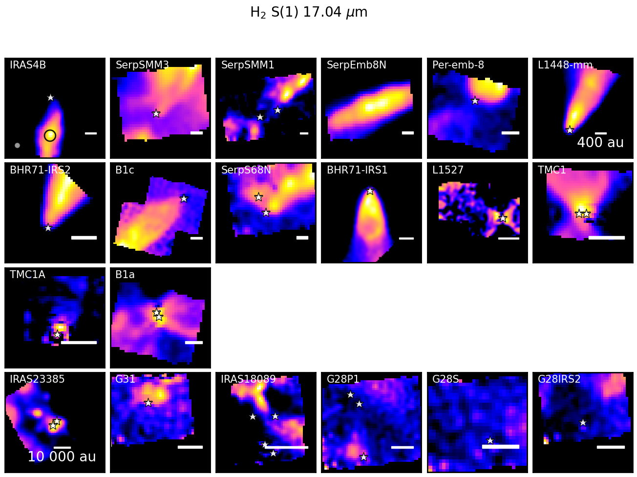
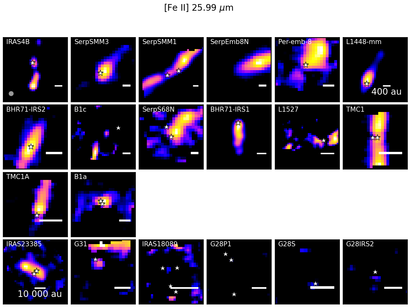
Figure 13: MIRI-MRS maps of the H₂ S(1) line at 17.03 $\mu$m toward all JOYS sources. The top three rows show the low-mass protostars in order of increasing $T_{\rm bol}$, whereas the bottom row shows the high-mass protostars. The white star(s) or arrow in each panel indicate the position of the protostar(s); for low-mass protostars those are derived from millimeter interferometry. A scale bar of 400 au is shown in each low-mass protostar panel, and a bar of 10000 au in each high-mass protostar panel. The beam size is indicated in the lower left corner of the first panel. Maximum colors in each panel are (in Jy km s^-1), from top left to bottom right, are, for low-mass: 0.59, 0.12, 0.03, 0.14, 0.08, 0.25, 0.08, 0.025, 0.041, 0.11, 0.006, 0.18, 0.31, 0.064; and for high-mass: 0.21, 0.02. 0.06, 0.021, 0.023, 0.027.

Figure 14: MIRI-MRS maps of the [Fe II] ⁴F${}_{7/2}-^{4}$F_9/2 line at 25.99 $\mu$m toward all JOYS sources. The top three rows show the low-mass protostars in order of increasing $T_{\rm bol}$, whereas the bottom row shows the high-mass protostars. The white star(s) or arrow in each panel indicate the position of the protostar(s); for low-mass protostars those are derived from millimeter interferometry. A scale bar of 400 au is shown in each low-mass protostar panel, and a bar of 10000 au in each high-mass protostar panel. The bright [Fe II] emission seen at the edges of some of the high-mass images are real. The beam size is indicated in the lower left corner of the first panel. Maximum colors in each panel are (in Jy km s^-1), from top left to bottom right, are, for low-mass: 1.18, 1.89, 15.65, 2.85, 0.62, 6.97, 1.41, 0.21, 0.56, 42.63, 0.17, 2.00, 3.72, 1.26; and for high-mass: 0.79, 0.80, 0.80, 0.80, 0.80, 0.80.

How do the results for Serpens SMM3 compare with those of other sources studied with JWST? Table 5 in Appendix E summarizes the main atomic and molecular lines that are seen in the MIRI spectra of protostars, together with their origin. It is well known that elements can be divided into volatile (e.g., noble gases), moderately volatile or semi-refractory (e.g., S, Cl), and refractory elements (e.g., Fe, Ni, Co) depending on their condensation temperatures (Lodders, 2003). Observations of elemental abundances in diffuse clouds using UV absorption lines show that the amount of depletion strongly varies between these categories, with volatile elements like Ne and Ar basically undepleted and refractory elements like Fe, Ni and Co heavily depleted by up to two orders of magnitude due to their incorporation into dust (Savage & Sembach, 1996; Jenkins, 2009). The semi-refractories are somewhere in between. The MIRI-MRS line images can indeed be divided along these different categories.

Figures 14 and 14 provide an overview of the H₂ S(1) line and one low-excitation fine-structure line of a refractory element, [Fe II] 25.99 $\mu$m, for the entire JOYS low- and high-mass protostar sample. In these figures, the low-mass sources NGC 1333 IRAS4A, SVS4-5 and HH 211 have not been included (see § 3); hence there are 14 rather than 17 low-mass panels. The full set of all line images will be presented in future papers, but the trends for low-mass sources are similar to those presented for Serpens SMM3.

A common theme is that a narrow jet is seen prominently in the [Fe II] lines at 5.34, 17.92, 24.52 and 25.99 $\mu$m, as well as in other refractory species, such as [Ni II] 6.63 $\mu$m and [Co II] 10.52 $\mu$m, which have been returned to the gas phase by shocks. Notably, [Fe I] 24.04 $\mu$m is exclusively detected in some Class 0 sources, not in Class I sources, and always in the jet. This finding is consistent with jets becoming more ionized with protostellar evolution (Nisini et al., 2015). The detection of both Fe and Ni lines in jets points to the presence of iron/nickel grains which do not have spectral features: this is the only way to discover the nature of Ni-containing dust (Henning, 2010; Manfroid et al., 2021).

Among the semi-refractories, the [S I] 25.24 $\mu$m line is bright and always elongated in the jet direction for Class 0 sources, where it also shows up prominently in bow shocks, like in SMM3. As for the refractories, it has been returned to the gas by shocks but it usually follows H₂ more closely than [Fe II]. If detected in Class I sources, [S I] emission is always compact on disk scales, and no longer associated with any jet (e.g., Tychoniec et al., 2024). In this context it has been suggested that sulfur-bearing species trace accretion shocks onto the disk (e.g., Sakai et al., 2014), but no convincing indications have yet been found that this is the case for [S I] (see § 8). A similar trend is seen with the other moderately volatile element [Cl I] 11.33 $\mu$m, but this line is much fainter so its detection is not clear for many targets.

Lines of the noble gases Ne and Ar show a mixed behavior: the strong [Ne II] 12.81 $\mu$m line often follows the jet, but it may also have a compact, spatially broader component centered close to the source, likely tracing the X-ray or (E)UV-irradiated cavities and cavity walls (see Figure 9 and Gieser et al. 2023b for the high-mass source IRAS 23385). The same holds for [Ar II] at 6.98 $\mu$m, but since its line is weaker than that of [Ne II] it is more difficult to separate the components. In contrast, [Ne III] 15.56 $\mu$m and [Ar III] 8.99 $\mu$m are primarily detected in Class I sources where they show only a moderately extended component, plausibly tracing the ionizing radiation (see also Gieser et al., 2023b; Tychoniec et al., 2024). The images of the noble gases demonstrate that not just elemental depletion but also local conditions (e.g., what is required to ionize Ne and Ar) determine the emission pattern.

Heated dust is detected through 20 $\mu$m continuum emission in some Class 0 sources such as HH 211, indicating that dust is launched in the jet (Caratti o Garatti et al., 2024). The question whether that dust is subsequently destroyed or not by shocks requires comparison of one of the refractory elements with a non-refractory one. Typically, sulfur lines are used for the latter (Nisini et al., 2002). However, the depletion behaviors of S and Cl are not yet well understood (see also above discussion): both species are undepleted in diffuse clouds with $A_{V}<$1 mag (Jenkins, 2009), but in dense clouds the bulk of S has been transformed into a more refractory component (e.g., Kama et al., 2019). Depletion of chlorine appears to be more modest in dense clouds based on observations of HCl (Blake et al., 1986). Thus, it is not a priori clear which element to take as the undepleted reference in determining the amount of depletion of elements in shocks. One of the noble gases (e.g., neon) that does not suffer any depletion could be a cleaner reference probe for abundances, as long as their line flux does not depend sensitively on other physical parameters. Another possibility for the case of S is to take H₂ itself (Anderson et al., 2013).

In the youngest Class 0 protostars, H₂ shows a mix of wide-angle wind and jet emission. The narrow jet is seen in the higher excitation H₂ lines such as S(5) and S(7), whereas emission from the lower-lying H₂ lines is dominated by the wide-angle wind (Fig. 10). For Class I sources, all H₂ lines fill the outflow cavity with the opening angle of the disk wind increasing with decreasing excitation (i.e., $J$ level) (Tychoniec et al., 2024). Molecular lines from CO, OH, HCO⁺ and CO₂ are also detected associated with the outflow (Tychoniec et al., 2024; Narang et al., 2024; van Gelder et al., 2024a) (see also § 6).

In conclusion, warm molecular gas is clearly present within the outflow cavity, not just as part of the cavity wall, and its velocity structure indicates that the gas is moving in the red- or blue-shifted directions. Whether H₂ lines are indeed tracing disk winds close to the source or simply gas inside the cavity that is heated and put in motion otherwise (e.g., by internal jet shocks or shocks with ambient material) would require velocity resolved line profiles and spatially resolved H₂ temperature and column density maps. Farther removed from the source, H₂ may also be mixed in by turbulence from the entrained outflow gas, and that gas may also be heated by UV radiation along the outflow cavity walls (e.g., Yıldız et al., 2015).

The atomic and molecular line images for the high-mass source IRAS 23385 +6053 show similar trends, both in refractories, volatiles and H₂ (Beuther et al., 2023; Gieser et al., 2023b). The patterns for the other high-mass sources are less clear from the images presented here: IRAS 18089 -1732 has a cluster of high-mass sources resulting in bright H₂ emission throughout the region, whereas the IRDC G28 positions show much weaker emission. The high-mass outflows and accretion will be studied in future papers.

5.3 Comparison with other JWST studies

The JOYS findings are consistent with results of low-mass Class 0 protostars from a number of other JWST programs. Early MIRI-MRS examples are the low-mass Class 0 sources IRAS 15398-3359 (CORINOS program; Yang et al., 2022; Salyk et al., 2024) (1.5 L_⊙) and IRAS 16253-2429 (0.2 L_⊙) (IPA program; Narang et al., 2024). Also, NIRSpec images of [Fe II] and H₂ (Federman et al., 2024) as well as CO (Rubinstein et al., 2024) ro-vibrational lines have been presented for all five IPA sources from low to high mass, for the Class 0 binary Serpens S68N (Le Gouellec et al., 2024a) and for the Class I source TMC1A (Harsono et al., 2023). MIRI and NIRSpec images of the Class I source HH 46 IRS (16 L_⊙) have been published by Nisini et al. (2024) as part of PROJECT-J; their Table 1 provides a useful overview of all atomic lines detected in HH 46.

A common finding of all of these early MIRI and NIRSpec results across low-mass Class 0 and I sources as well as high-mass protostars, is the presence of highly collimated jets, most notably seen in the various [Fe II] lines and in the highest excitation H₂ pure rotational and ro-vibrational lines. Wider angle winds are traced by the lowest H₂ pure rotational lines, as found within JOYS (Tychoniec et al., 2024). Lines of other refractory species as well as noble gas (Ne, Ar) lines are also commonly detected, with the latter species often showing a different distribution from either [Fe II] or H₂, consistent with what is found in JOYS. Analyses of the nested physical structure of the Class I source DG Tau B and a small sample of young Class II jets and winds are presented in Delabrosse et al. (2024); Pascucci et al. (2025). Some H I emission is seen also off source in both NIRSpec and MIRI data (e.g., Neufeld et al., 2024), demonstrating that not all the H I recombination line luminosity is due to the accretion column onto the star.

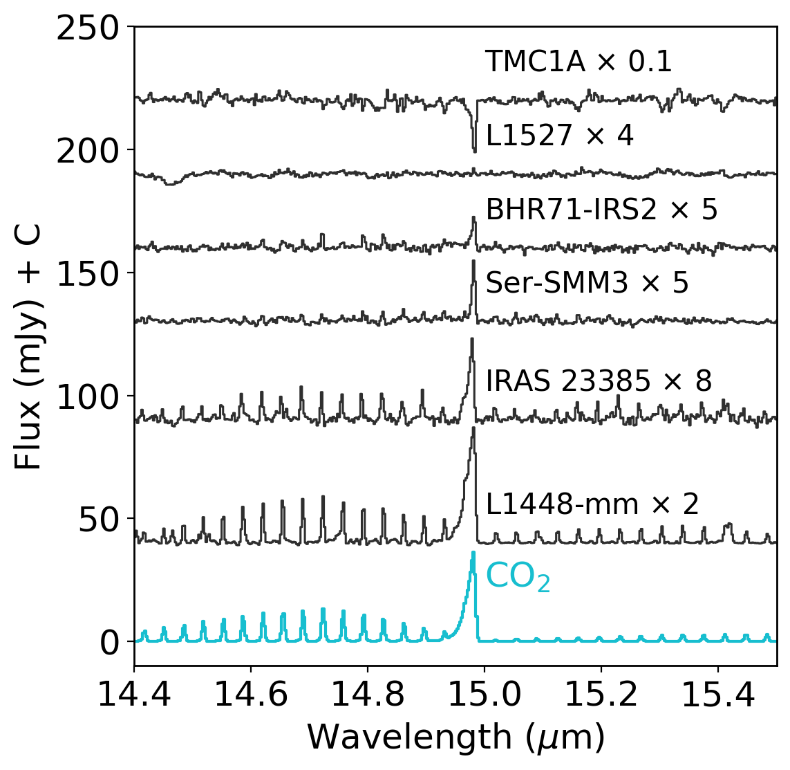
Figure 15: Comparison of CO₂ 15 $\mu$m emission and absorption toward several low- and high-mass protostars. The bottom panel shows a model spectrum at $T$=120 K (best fit for L1448-mm), with the $P$-branch extincted by CO₂ ice.

6 Hot cores and dense molecular shocks: chemistry

MIRI-MRS spectra of the first observed JOYS target, the high-mass binary protostar IRAS 23385+6053, demonstrated that many gas-phase molecular lines can be detected at the source positions and that not just $Q$ branches but also individual $P$- and $R$- branches (see Figs. 4 and 5) can be seen (Francis et al., 2024). The MIRI-MRS spectra at central positions of the low-mass JOYS sources have been analyzed in a recent overview paper of molecular lines by van Gelder et al. (2024a). Rich spectra containing lines of up to 13 different molecules (including isotopologs) are seen toward 3 out of 16 sources with mid-infrared continuum, two in emission (L1448-mm and BHR71-IRS1) and one in absorption (B1-c). Other sources show primarily H₂O, CO, CO₂ and/or OH, but not C₂H₂, HCN, SO₂ or SiO. The Serpens SMM3 source, discussed extensively in § 5 as an example protostellar source, shows only CO₂ emission (Fig. 15) but no H₂O. For most sources and molecules, no significant ($>10$ km s^-1) velocity offsets are seen, except for BHR71-IRS1 (all lines) and L1448-mm (H₂O and SiO). We here highlight the main results for both low- and high-mass sources and put them in the context of the various scenarios of hot core chemistry, dense molecular shocks and winds. See § 2.3 and § B.2 for background information.

6.1 From CO₂ to SO₂: cool emission

CO₂.

CO₂ gas-phase lines at 15 $\mu$m are seen in emission toward IRAS 23385+6053 (Beuther et al., 2023), rather than in absorption as found for the sample of high-mass protostars surveyed with ISO-SWS (Boonman et al., 2003b). This difference is likely due to the much higher spatial resolution of JWST, being able to detect the weak emission on source, whereas any emission in the large ISO-SWS beam was overwhelmed by the larger scale absorption against the extended infrared continuum. For IRAS 23385, the resolved $R-$ and $Q-$ branches provide an accurate temperature of $\sim$120$\pm 10$ K (Francis et al., 2024). One early lesson is that gas-phase lines can be differentially affected by foreground ice absorption; this holds in particular for the $P-$branch lines of CO₂ being obscured by CO₂ ice, but the same effect is also seen for other species such as SO₂ and H₂O in the 6–8 $\mu$m range, in addition to the overall extinction (van Gelder et al., 2024b). This finding also puts direct constraints on the location of the emission: it must originate from behind where the bulk of the ice is located.

Figure 15 shows a blow-up of the gas-phase CO₂ detections in several low-mass sources at their central position in comparison with IRAS 23385. CO₂ is seen in 11 out of the 16 sources studied in van Gelder et al. (2024a), with 4 out of 11 in absorption (see also Tychoniec et al., 2024). Where detected, the CO₂ emission is cool, as in IRAS 23385, with typical rotational temperatures of 100–200 K (compare with Fig. 5). For CO₂ in absorption, the temperatures are somewhat higher, up to 300 K. The temperatures derived from CO₂ emission in protostars are lower than the values up to $\sim$400 K found in protoplanetary disks (e.g., Grant et al., 2023; Vlasblom et al., 2024). Also, the hot bands are never detected in protostars, consistent with low temperatures and lower densities (see Fig. 5).

Since CO₂ does not have a permanent dipole moment, the rotational populations in $v=0$ should be thermalized and reflect the kinetic temperature of the gas. The rotational populations in $v=1$, measured with JWST, should be similar if infrared pumping is indeed the main mechanism for exciting the molecule (see § 3.5). Several findings therefore argue in favor of a hot core origin of CO₂ rather than in shocks (van Gelder et al., 2024a): (1) temperatures of 100–200 K consistent with ice sublimation; (2) lack of a velocity shift compared with the source velocity; (3) similar gas and ice CO₂/H₂O abundance ratios, and (4) location of the emission behind the ice absorption, i.e., closer to the protostar.

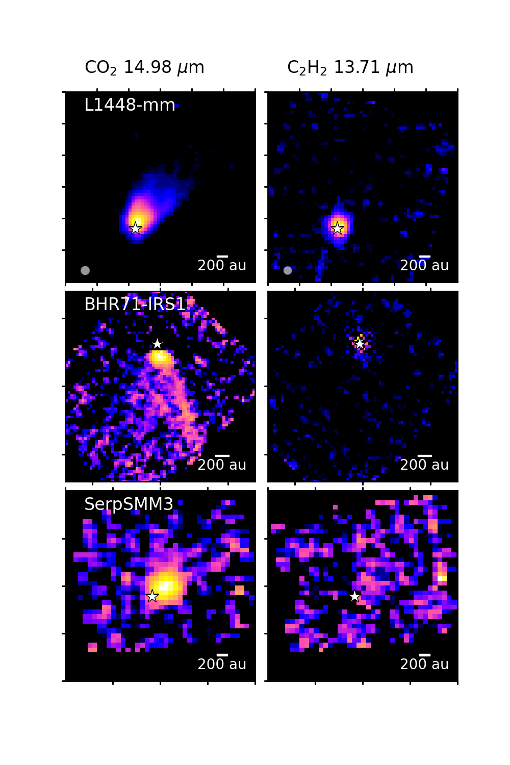
Figure 16: Maps of CO₂ 15 $\mu$m and C₂H₂ 13.7 $\mu$m emission toward three low-mass sources. Note that CO₂ is generally extended along the outflow whereas C₂H₂ is centered on source, whose location is indicated by the white star. The beam size is indicated in the lower left corner.

Note, however, that in some sources with prominent outflows CO₂ emission is also found to be extended along the outflow over distances up to 1000 au, as illustrated in Figure 16 (see also Boonman et al., 2003c; Sonnentrucker et al., 2007). One likely scenario is that the observed gaseous CO₂ away from the hot core is enhanced by ice sputtering of the dense and cold material along the outflow cavity walls or in a slow wind, and subsequently excited by infrared radiation from the source escaping through the outflow cavity. Warm gas-phase chemistry, especially through the CO + OH $\to$ CO₂ + H reaction, which is particularly effective in the 100–300 K range, can contribute as well (e.g., van Dishoeck et al., 2023).

C₂H₂ and HCN.

Both molecules are detected toward IRAS 23385 and other high-mass protostars, as well as toward a few low-mass protostars (van Gelder et al., 2024a). Excitation temperatures from emission features are similarly low as for CO₂, 100–200 K, again lower than the values up to 600 K found for C₂H₂ and up to 900 K for HCN in protoplanetary disks around T Tauri stars (e.g, Gasman et al., 2023; Grant et al., 2023; Temmink et al., 2024a; Schwarz et al., 2024; Colmenares et al., 2024). In contrast with CO₂, neither of these two molecules are seen along the outflow (Fig. 16), or toward outflow positions well offset from the high mass protostellar sources as was the case in Orion (Boonman et al., 2003c). In low-mass outflows, such as HH 211, C₂H₂ and HCN are also not seen at any of the strong knot positions. There is one clear exception, the NGC 1333 IRAS4B shock, discussed in § 6.3, and one other spot near Serpens SMM1. The fact that C₂H₂ and HCN are generally not extended makes a hot core origin most plausible for these molecules, with high temperature gas-phase reactions rather than ice sublimation dominating the formation of C₂H₂ and HCN (Francis et al., 2024; van Dishoeck et al., 2023) (see also models below).

CH₄.

Methane gas is not readily seen toward protostars. Analysis of the JOYS low-mass sample reveals detections only in the two line-rich sources (B1-c, L14448-mm), as well as in the source SVS4-5, which is likely a disk (van Gelder et al., 2024a). In the former two sources, CH₄ is again cool, with temperatures of 100–200 K, suggesting a similar hot core origin as the other organic molecules. In disks around T Tauri stars, CH₄ is also seldom seen, with only two tentative detections reported (Colmenares et al., 2024; Temmink et al., 2025). In contrast, rich CH₄ line forests are prolific in many disks around very low-mass stars and brown dwarfs, even if not always easily distinguished due to line overlaps with C₂H₂ (e.g., Arabhavi et al., 2024; Kanwar et al., 2024).

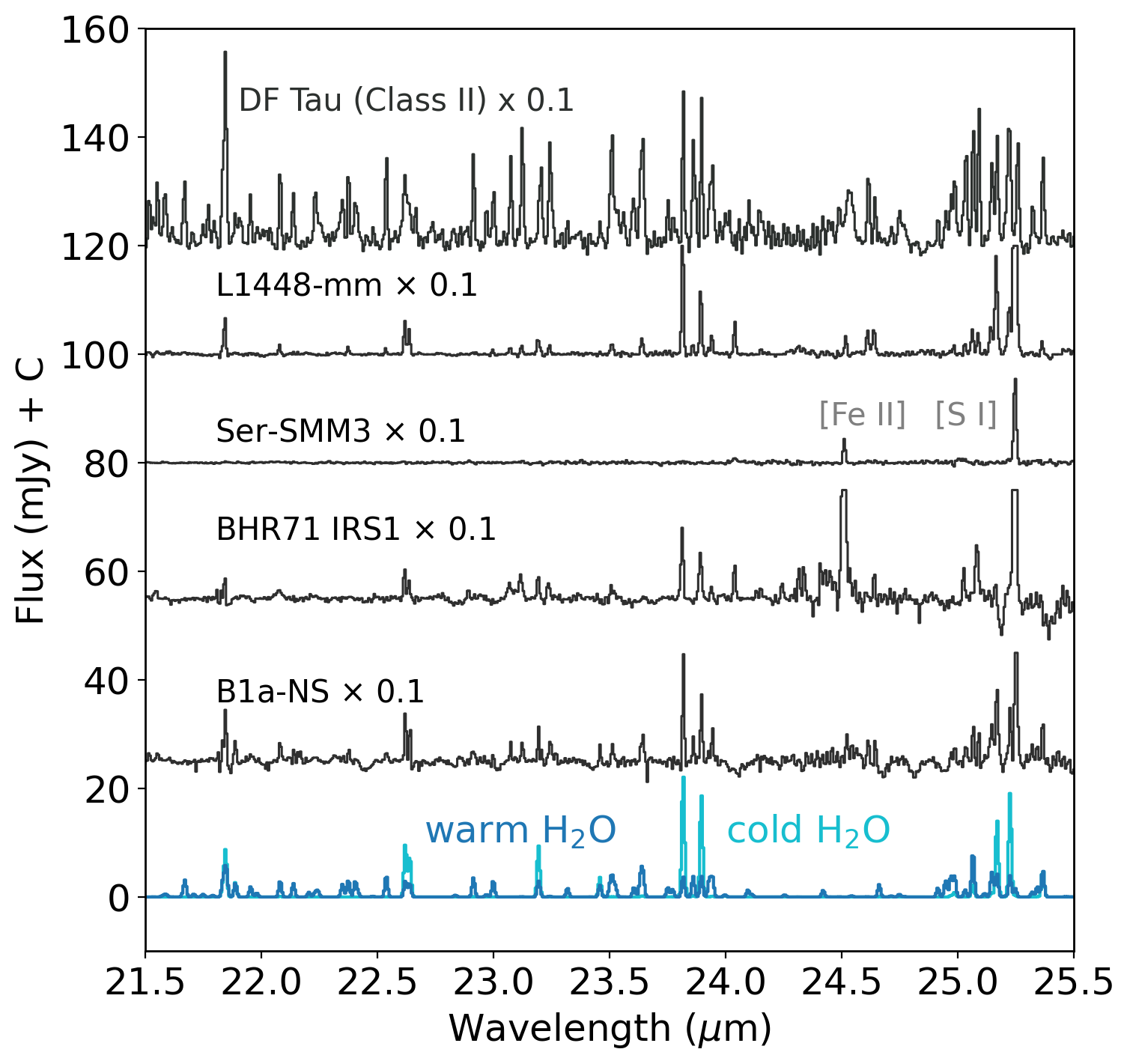
Figure 17: Comparison of H₂O emission toward several low-mass protostars at long wavelengths in MRS Channel 4. B1-a-NS is a Class I source, the other sources are Class 0 sources, including SMM3. The bottom panel shows warm and cold water model spectra at $T_{\rm rot}$=370 K (dark blue) and 160 K (light blue). The observed emission in protostars is dominated by the colder component. For comparison, the spectrum of a Class II disk, DF Tau, is shown at the top, illustrating that this disk also has strong warm water emission (Grant et al., 2024).

H₂O.

Water emission is surprisingly weak toward IRAS 23385, both through its vibration-rotation (5.5–7.5 $\mu$m) and pure rotational ($>13$ $\mu$m) lines. Toward one of the two sources in the binary, H₂O is also seen in absorption at a higher temperature of 550 K, more characteristic of winds or the inner warm disk midplane (Barr et al., 2020). H₂O emission and absorption is also seen in other high-mass protostars (see example of IRAS 18089 in § 7).

The low-mass protostars do not show prominent water emission lines, which is very different from the water emission forest seen in several more evolved Class II disks (e.g., Gasman et al., 2023; Pontoppidan et al., 2024b; Temmink et al., 2024a; Banzatti et al., 2025). However, upon close inspection, H₂O is detected in most low-mass protostars, either in the ro-vibrational band or in the pure rotational lines or in both, in absorption or emission (van Gelder et al., 2024a). These data indicate the presence of water at two temperatures: a cool temperature of 100–200 K, and a warmer component at 400–500 K, likely reflecting both a hot core and shock component. Figure 17 shows prominent water lines at longer wavelengths in the MIRI-MRS Channel 4, comparing a few Class 0 and I sources with the line-rich Class II disk DF Tau (Grant et al., 2024). In particular, the quartet of lines around 23.8 $\mu$m has been found to be a good indicator of the presence of cold versus warm water as shown by Banzatti et al. (2023, 2025); Temmink et al. (2024a). The fact that the warm water lines are clearly suppressed in the protostellar sources indicates that the H₂O excitation temperature of water is indeed low. In contrast, the spectrum of a water-rich Class II source, DF Tau, has prominent warm and cold water lines in this wavelength range: all four lines rather than just two lines of the 23.8 $\mu$m quartet are seen.

Note that the two temperature components of water found in protostellar sources are not necessarily the same as the hot, warm and cold(er) components found in Class II disks where they have been associated with temperature gradients in the disk surface in the inner few au and water enhancement at the snowline (Banzatti et al., 2023, 2025; Gasman et al., 2023; Temmink et al., 2024a; Romero-Mirza et al., 2024): while there may be a similar water vapor enhancement in hot cores around 100 K, H₂O is likely to be subthermally excited at the much lower densities in protostellar environments whereas the H₂O ro-vibrational band can be pumped by infrared radiation. Comparison with water in hot cores imaged with ALMA through lower excitation pure rotational lines of H${}_{2}^{18}$O and HDO (e.g., Persson et al., 2016; Jensen et al., 2019) will be done in future studies.

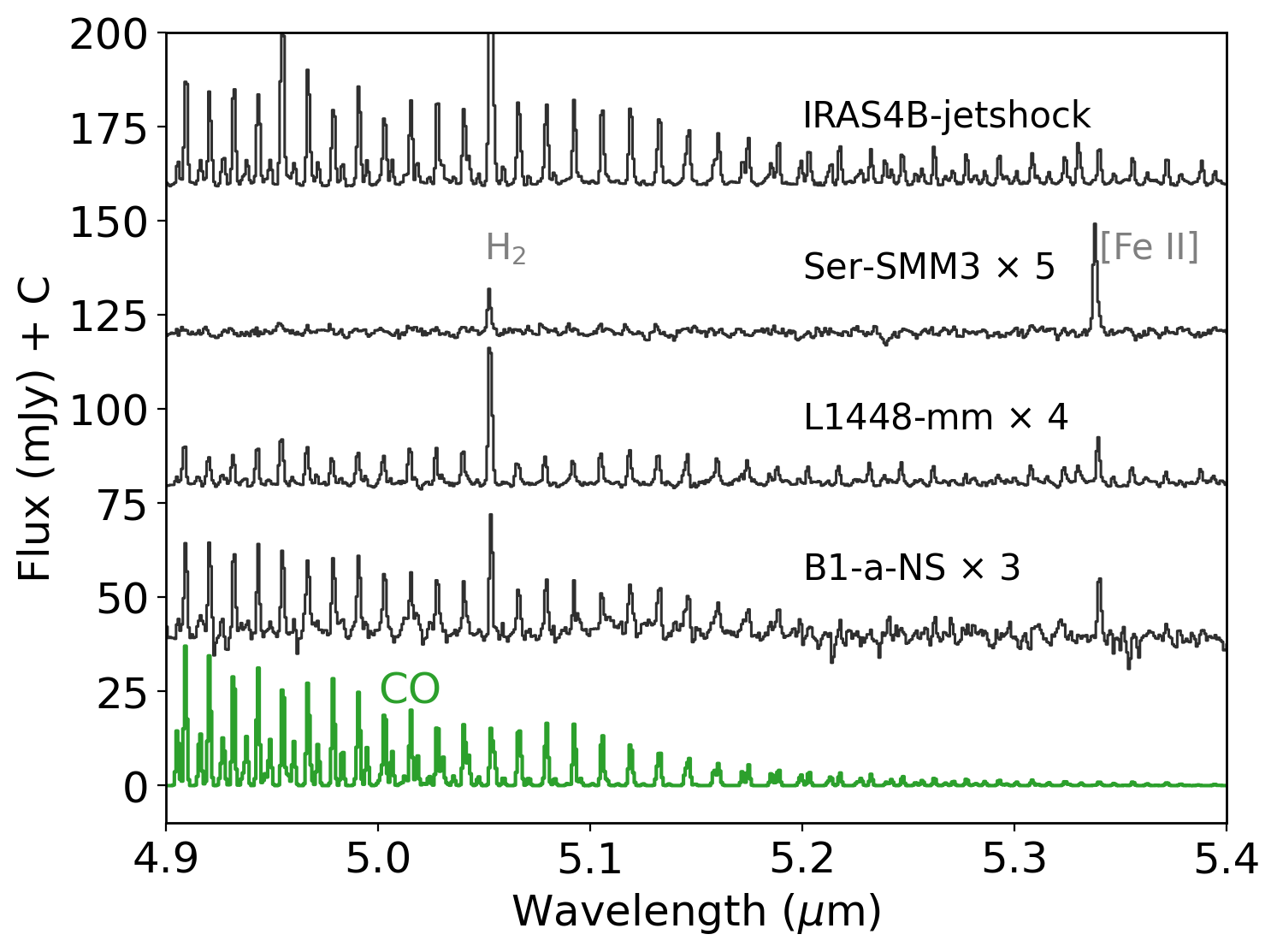
Figure 18: Comparison of CO $v=1-0$ 5 $\mu$m emission toward several low-mass protostars. L1448 and SMM3 are Class 0 protostars, B1-a-NS is a Class I source, and the spectrum of NGC 1333 IRAS4B is taken at a shock knot position well off source (see Fig. 20). The bottom panel shows an optically thick CO model spectrum at $T$=1500 K.

CO.

CO emission is seen in about half the MIRI spectra of protostars in the 4.9–5.2 $\mu$m range, showing the tail of the $v=$1–0 $P-$branch with $J_{\rm up}\geq 23$ (Fig. 18) (see also Salyk et al., 2024). When detected, it always indicates a high temperature (Fig. 4). A naive rotation diagram analysis assuming optically thin lines would imply $\sim$2000 K, but the actual kinetic temperature can be substantially lower, $\sim$1000 K if the CO emission is optically thick (see discussion in Herczeg et al., 2011; Francis et al., 2024; Rubinstein et al., 2024; Le Gouellec et al., 2024b). Such emission could be consistent with the innermost disk region, as in Class II sources (e.g., Banzatti et al., 2022), but it can also be associated with the disk surface (Arulanantham et al., 2024) or shock knots (see § 5) (Federman et al., 2024). Indeed, spectrally resolved ground-based CO data for Class I sources often show wind and outflow absorption in ¹²CO $v$=1-0 profiles that could mask any emission in spectrally unresolved data (Herczeg et al., 2011). High extinction by the inner envelope could also hide CO emission in sources where it is not seen.

SO₂

. JWST has detected mid-infrared emission of SO₂ at 7.3 $\mu$m for the first time in a low-mass protostar (van Gelder et al., 2024b). It is seen toward the Class 0 protostar NGC 1333 IRAS2A, a source that is part of JOYS+ in program 1236 (PI: M. Ressler). Inspection of the full JOYS low-mass sample spectra shows that this band is not commonly seen, only toward L1448-mm in emission and B1-c in absorption (van Gelder et al., 2024a).

SO₂ is one of the few molecules that can be observed with both JWST and ALMA since it has a permanent dipole moment. Interestingly, for IRAS2A the excitation temperature derived from the mid-infrared data, $\sim 100$ K, is the same as that derived from the wealth of SO₂ millimeter lines imaged with ALMA on scales of $\sim 60$ au radius as presented in van Gelder et al. (2024b) using data from program 2021.1.01578 (PI: B. Tabone). Similarly low temperatures are found for the two JOYS sources. To what extent does this excitation temperature $T_{\rm rot}$ reflect the kinetic gas temperature $T_{\rm kin}$?

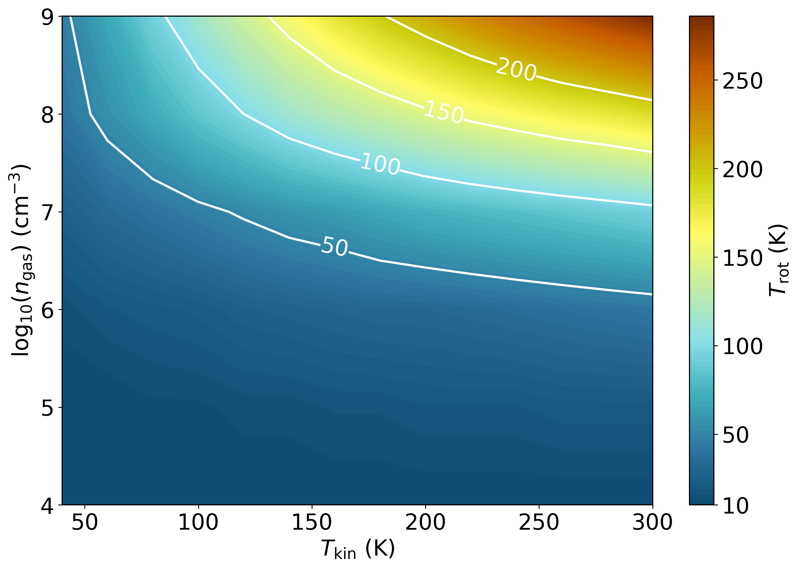
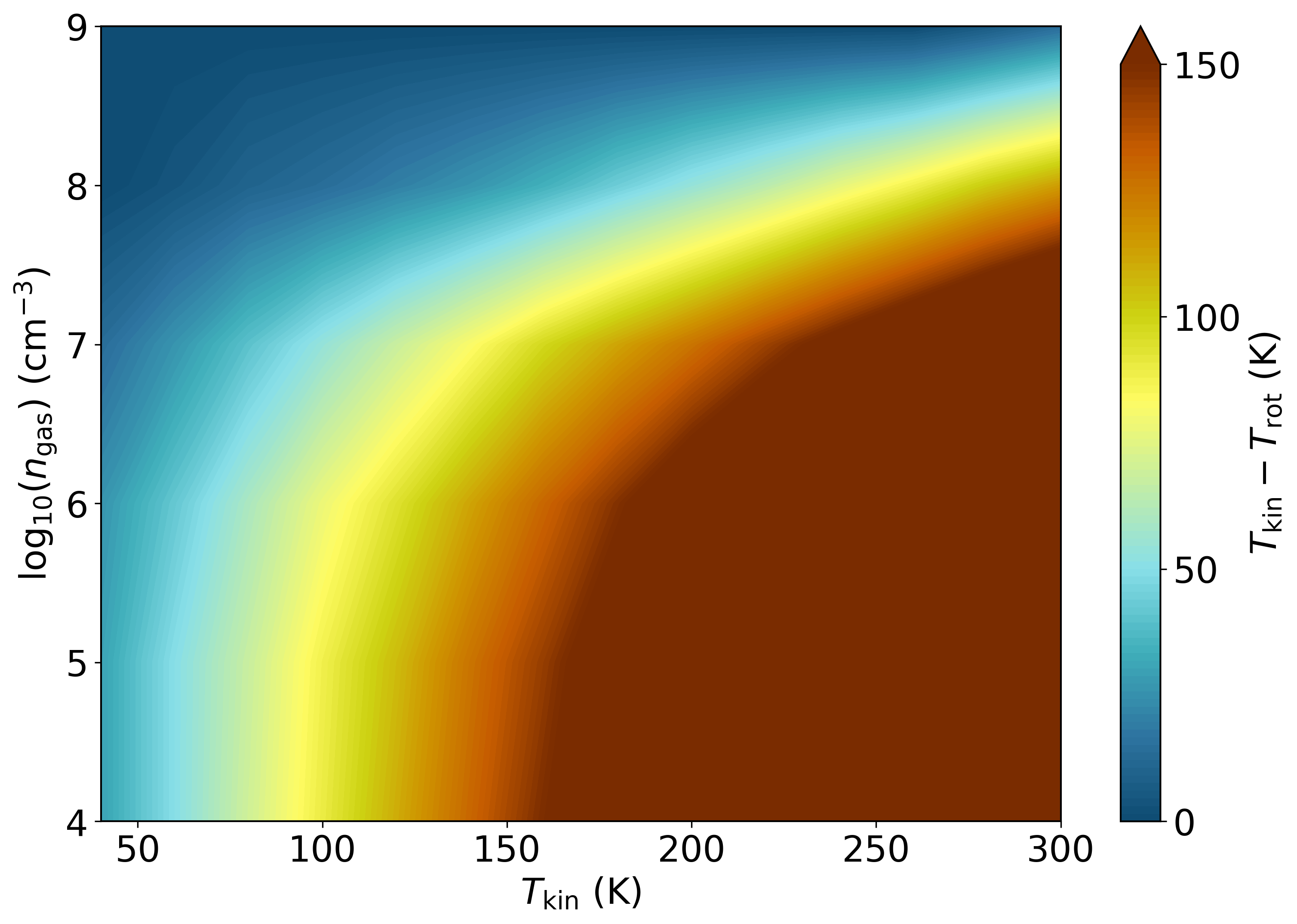
Figure 19: Top: SO₂ rotational temperature $T_{\rm rot}$ within $v$=0 as function of kinetic temperature $T_{\rm kin}$ and density $n$(H₂) obtained from non-LTE calculations. Bottom: Difference between $T_{\rm kin}$ and $T_{\rm rot}$. Note the large deviations at low densities ($<10^{7}$ cm^-3).

Within $v$=0, the level populations are determined by a mix of collisional (de-)excitation and radiative decay. A non-LTE excitation calculation using RADEX (van der Tak et al., 2007, 2020) with collisional rate coefficients from Balança et al. (2016) is adopted to compute $T_{\rm rot}$ and the difference between $T_{\rm kin}$ and $T_{\rm rot}$ as a function of kinetic temperature and H₂ density $n$. $T_{\rm rot}$ is obtained by fitting a rotation diagram to the model results for the same lines as observed with ALMA in IRAS2A. Figure 19 shows that at low densities ($<10^{7}$ cm^-3) the excitation is subthermal, $T_{\rm rot}<<T_{\rm kin}$. However, typical envelope densities on scales of $<$100 au are $10^{7}-10^{9}$ cm^-3 (Jørgensen et al., 2004; Notsu et al., 2021) for which differences $T_{\rm kin}-T_{\rm rot}$ are smaller.

Thus, the temperatures derived from the MIRI-MRS data should be representative of the gas in which SO₂ resides. The number of molecules inferred from LTE slab models, however, is not: it is overestimated by a factor of 10⁴ when compared with the ALMA results. The mid-infrared lines are clearly pumped by scattered IR radiation with a brightness temperature of $\sim$180 K, substantially higher than the rotational temperature (van Gelder et al., 2024b). When the infrared pumping is included, the number of molecules derived from the JWST and ALMA data are consistent. Combined with the small millimeter line width and lack of a velocity shift, a hot core rather than an accretion shock origin seems most likely for SO₂. This study emphasizes the synergy between JWST and ALMA for molecules with a dipole moment.

Although the importance of subthermal excitation and infrared pumping is highlighted here for the case of SO₂ in IRAS2A, Figure 19 is representative for other molecules with a dipole moment such as HCN and H₂O. The analysis in van Gelder et al. (2024a) also shows the importance of infrared pumping for other molecules and sources.

OH.

As noted in § 5, mid-IR OH emission has been detected with Spitzer in bow-shocks (Tappe et al., 2008, 2012) and other environments with strong UV irradiation such as the surface layers of protoplanetary disks (Carr & Najita, 2014). It is now also prominently seen with JWST in low-mass protostars at the source position (van Gelder et al., 2024a) and at (bow) shock positions (Neufeld et al., 2024; Caratti o Garatti et al., 2024), as well as in an irradiated disk (Zannese et al., 2024). Class II protoplanetary disks commonly show OH (e.g., Gasman et al., 2023; Temmink et al., 2024a; Schwarz et al., 2024; Vlasblom et al., 2025) although mostly at the longer wavelengths. In the high-mass JOYS sample, OH emission is only prominent in IRAS 23385 (Francis et al., 2024) although it is detected in some other sources (Reyes et al. in prep.).

The OH lines originate from extremely high rotational states, with rotational quantum numbers up to $N$=40 ($E_{\rm up}=40000$ K). This phenomenon results from photodissociation of H₂O through its second electronically excited state, the ${\tilde{B}}$ state, producing OH in very high $N$ states which then cascade down through pure rotational transitions to the ground state, a process that has been well studied in the laboratory and through quantum chemical calculations (e.g., Harich et al., 2001; van Harrevelt & van Hemert, 2000), see summary in Tabone et al. (2021). This process requires UV photons at 1140 –1430 Å, a wavelength range that includes Lyman $\alpha$ at 1216 Å, and is thus a direct diagnostic of the strength of the UV radiation multiplied by the number of H₂O molecules (Tabone et al., 2023). The OH “prompt emission” occurs primarily at 9-11 $\mu$m with a characteristic asymmetry in the emission of the $\Lambda$-doublet lines. At longer wavelengths ($>13$ $\mu$m, depending on temperature), chemical pumping through the O + H₂ $\to$ OH($v,J$) + H reaction contributes. Most of the JOYS sources show only these longer wavelength OH lines indicative of warm gas-phase chemistry (Francis et al., 2024; van Gelder et al., 2024a), although prompt emission is seen in a few JOYS sources (TMC1, BHR71-IRS1) besides HH 211. The implications of the presence or absence of 9–11 $\mu$m OH emission for the amount of UV and water remain to be quantified. Previously inferred values of the enhancement factor $G_{o}$ compared with the interstellar radiation field are of order $10^{2}-10^{3}$ on scales of $\sim$1000 au using other tracers (Yıldız et al., 2015; Benz et al., 2016).

Table 3: Column density ratios of key molecules observed toward the low-mass protostar B1-c

Species	Observeda	Model	Model	Model	Model	Model	Model
		150 K	150 K	300 K	300 K	600 K	600 K
		no X-rays	$L_{X}=10^{29}$	no X-rays	$L_{X}=10^{29}$	no X-rays	$L_{X}=10^{29}$ erg s-1
CO2/H2O	0.22	0.025	0.27	0.0016	0.0025	0.0012	0.0029
HCN/H2O	0.08	0.024	0.0001	0.037	0.037	0.063	0.086
C2H2/H2O	0.05	$<$0.0001	0.0003	$<$0.0001	0.0054	0.0001	0.0069
CH4/H2O	0.10	0.039	0.028	0.020	$<$0.0001	0.048	0.013
NH3/H2O	0.04	0.05	0.0001	0.062	0.016	0.10	0.069
C2H2/HCN	0.64	0.0001	3.4	0.0004	0.15	0.002	0.08
C2H2/CO2	0.21	0.0001	0.001	0.008	2.2	0.10	240

^a Observed column densities taken from Table H.4 of van Gelder et al. (2024a), using the warm H₂O column of $4.4\times 10^{18}$ cm^-2 as reference. Observational uncertainties in the ratios are about 50%.

Other molecules.

van Gelder et al. (2024a) report the first mid-infrared detection of NH₃ in a protostar, seen in absorption toward B1-c. The NH₃/H₂O column density ratio of 0.04 is again consistent with ice sublimation in a hot core. Other first detections toward a low-mass protostar include CS absorption (B1-c), and C₄H₂ and SiO emission (L1448-mm). The ¹³C isotopologs of CO₂ and C₂H₂ are also seen for these two sources.

In summary, the relatively low temperatures of 100–200 K (somewhat higher in absorption) coupled with the lack of velocity shifts point toward a hot core origin for the bulk of the molecules. This is further strengthened by the similarity of gas and ice abundances relative to H₂O for molecules seen in ices: CO₂, CH₄ and NH₃, especially in the case of B1-c (see van Gelder et al., 2024a, and below). For L1448-mm and BHR71-IRS1, however, some molecules like H₂O are clearly associated with the outflow based on velocity offsets.

6.2 Molecular abundances: hot core chemistry

How do the inferred molecular abundances compare with models? The cleanest case for studying hot core chemistry is that of B1-c, for which the lines are in absorption and are therefore not affected by radiative pumping. Also, isotopologs are detected to correct for optical depth. For emission lines, determination of column densities and abundances is complicated by the fact that IR radiative pumping needs to be properly accounted for: column densities can be too high by orders of magnitude if LTE excitation at the same low temperature that characterizes the rotational distribution is assumed for populating the vibrational levels (see case of SO₂ above).

Table 3 summarizes some key column density ratios of molecules. Determination of the fractional abundances with respect to H₂ is complicated by the fact that there is no clean tracer of the amount of 100–300 K molecular gas, hence warm H₂O is taken as a reference. Values are taken from Table H.4 of van Gelder et al. (2024a) and have a typical uncertainty of 30%. This can be higher if the optical depth of the lines is underestimated. Specifically, for CO₂ and C₂H₂, the column densities of ¹³CO₂ and ¹³C₂H₂ multiplied by 70 respectively 35 are used in Table 3. For CO₂ this value is a factor of three higher than that found from ¹²CO₂. The use of ratios implicitly assumes that the molecules are present in the same gas.

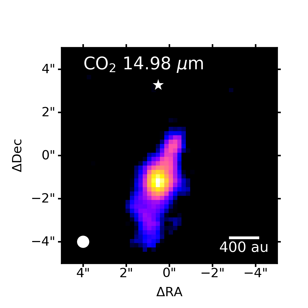
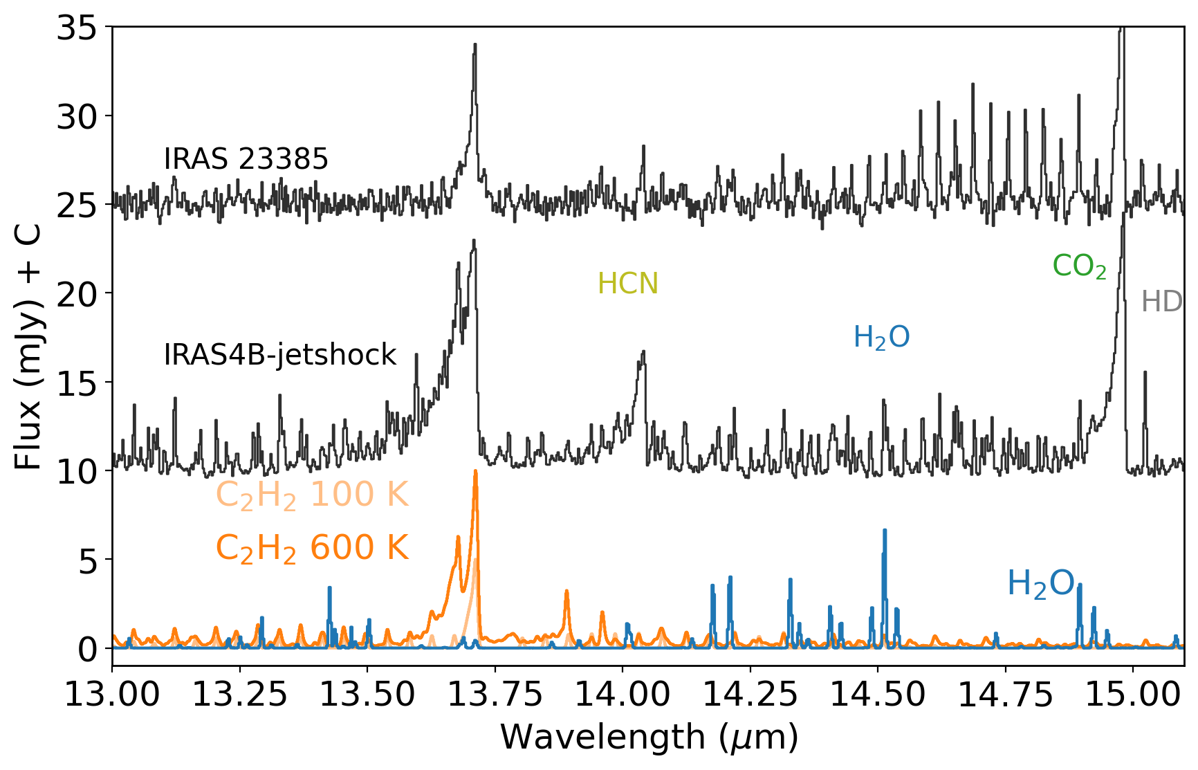
Figure 20: Left: MRS image of the CO₂ 15 $\mu$m band toward NGC 1333 IRAS4B showing the peak emission to be $\sim$1000 au ($\sim 4^{\prime\prime}$) offset from the source itself, whose position from millimeter interferometry is indicated by the white star. The beam size is indicated in the lower left corner. Right: MIRI-MRS spectrum of the NGC 1333 IRAS4B jet “knot” position in the 13–15 $\mu$m range highlighting its rich spectrum including hot C₂H₂ (600 K). For comparison, the spectrum of the high-mass protostar IRAS 23385, which shows only cold C₂H₂, is presented (Francis et al., 2024). The model spectra at the bottom show the contributions from C₂H₂ (100 and 600 K) and H₂O (280 K) in this wavelength range.

The chemistry in hot cores has been studied in a number of models over the past decades that start with the sublimation of ices at $t=0$ above their sublimation temperature (typically taken to be 100 K, representative of H₂O) and then follow the gas-phase chemistry for up to $10^{5}$ yr (e.g., Charnley et al., 1992; Doty et al., 2004). It is well known that the abundances of some molecules are particularly sensitive to temperature, most notably HCN and C₂H₂ being significantly enhanced in warmer gas (Doty et al., 2002). In contrast, CO₂ production through CO + OH $\to$ CO₂ + H is halted at $\sim$250 K when the OH + H₂ reaction takes over (see discussion in van Dishoeck et al., 2023). Another parameter that plays a role in setting the relative abundances is the X-ray luminosity. X-rays can both destroy molecules (e.g., water) and enhance molecules (e.g., C₂H₂) (Stäuber et al., 2005, 2007; Notsu et al., 2021).

Table 3 lists the results of the gas-grain chemistry model of Notsu et al. (2021) using the envelope structure of NGC 1333 IRAS2A derived by Kristensen et al. (2012) at $r$=60 au. This position is just inside the water snowline ($\sim$150 K) where the hot core starts and the density is $2\times 10^{8}$ cm^-3. Such conditions are also representative of the B1-c envelope inside its snowline, even though it lies at somewhat smaller radii since B1-c is less luminous than IRAS2A. Values without X-rays and for $L_{X}=10^{29}$ erg s^-1 are tabulated. The model uses a detailed chemical network taken from Walsh et al. (2012, 2015).

The adopted X-ray luminosity of $L_{X}=10^{29}$ erg s^-1 is consistent with observations and chemical analyses of low-mass protostars (Benz et al., 2016) and turns out to be a “sweet spot” where the gas-phase CO₂ and C₂H₂ abundances are enhanced by one respectively two orders of magnitude at 150 K. Thus, this choice maximizes C₂H₂. H₂O and CH₄ are decreased by less than a factor of two for this value, but HCN and NH₃ are lower by more than two orders of magnitude, explaining the dramatic changes in the abundance ratios of, for example, C₂H₂/HCN in models with and without X-rays. For higher values of $L_{X}$, the abundances of all these six molecules decrease sharply. The use of H₂O as a reference introduces some uncertainties since its observed overall hot core abundance with respect to H₂ has been found to be less than the canonical value of $2\times 10^{-4}$ in models without X-rays (Persson et al., 2014, 2016). This observed low water abundance has, in fact, been one of the main motivations for introducing X-rays into the models (Stäuber et al., 2007; Notsu et al., 2021).

The overall conclusion of Table 3 is that hot core models of ice sublimation and gas-phase chemistry with modest X-rays reproduce the observed abundance ratios reasonably well within the model uncertainties of up to an order of magnitude. However, C₂H₂ is consistently underproduced by orders of magnitude at temperatures of only 150 K.

This underabundance of C₂H₂ has been noted before, also in the context of explaining its observed high abundances in high-mass protostars and even in deeply obscured (ultra)luminous infrared galaxies (Lahuis et al., 2007; Buiten et al., 2025). Temperature is clearly the one parameter that affects C₂H₂ most. Table 3 therefore also includes model abundances for temperatures of 300 and 600 K at the same density. These results show that the C₂H₂ abundance is indeed boosted at higher temperatures, especially in the presence of X-rays, although the observed high C₂H₂/H₂O ratios are not yet reached. Note that the observed rotational temperature of C₂H₂ in absorption toward B1-c is 285 $\pm$ 25 K, i.e., just consistent with the temperature regime at which C₂H₂ is significantly enhanced. HCN is increased as well with temperature, but not as strongly as C₂H₂. As expected, the CO₂ abundance is lower at $T>300$ K, since OH is now driven into H₂O. Taken together, these results should be viewed as illustrative of the parameter regime that can explain the observed column density ratios. No single position model can explain all the column density ratios and the hydrocarbon chemistry remains to be fully understood. Explaining high C₂H₂ abundances derived from emission lines in hot core regions, where this molecule has a low rotational temperature of only $\sim$150 K, would be a significant challenge if such temperatures were representative of the kinetic gas temperature. Source-specific depth-dependent models are needed to test whether the type of models presented here can reproduce both absolute and relative column densities. Note also that these models do not consider any contribution from shocks; see § 6.3 for detection of strong and warm C₂H₂ emission in at least one jet shock position that may have a different explanation.

6.3 NGC 1333 IRAS4B: dense shock

Dense non-dissociative shocks can also emit copious molecular emission of molecules other than H₂ (Draine et al., 1983; Kaufman & Neufeld, 1996). Indeed, extended warm H₂O emission has been imaged with Herschel-PACS in significant samples of low- and high-mass protostars showing both emission on and off source on scales of several thousand au (e.g., Nisini et al., 2010; Tafalla et al., 2013; Karska et al., 2013, 2018; van Dishoeck et al., 2021). Is this seen in our data at any shocked positions off source? The HH 211 MRS map revealed bright OH prompt emission at the outer bow shock together with CO, H₂O and weak HCO⁺ and CO₂ (see Fig. 7 of Caratti o Garatti et al. 2024), but no emission from other molecules. Also, in contrast with the extended H₂O emission mapped by Herschel-PACS (Dionatos et al., 2018), no H₂O emission is found with MIRI at other HH 211 positions than the outer bow shock.

A special case within JOYS is formed by the Class 0 low-mass protostar NGC 1333 IRAS4B in Perseus ($d$=293 pc, $L$=4.4 L_⊙, Table 1). This source attracted attention by Spitzer since its mid-infrared IRS spectrum shows a very rich H₂O spectrum with an excitation temperature of $\sim$170 K. It was speculated that these warm bright H₂O lines were due to a slow accretion shock liberating water at the envelope-disk interface in this young system (Watson et al., 2007). The subsequent longer wavelengths Herschel-PACS spectrum of this source taken with 9^′′ spaxels was found to be equally rich in H₂O and other far-infrared lines. However, the Herschel Nyquist-sampled spectral maps suggested the bulk of the emission to come from a position $\sim 5^{\prime\prime}$ south of the central source position as measured by millimeter interferometry, along the blue-shifted outflow lobe (Herczeg et al., 2012). The central source was concluded to be too heavily extincted even at these longer wavelengths. Rather than high-density ($\geq 10^{11}$ cm^-3) thermalized emission suggested by Watson et al. (2007), subthermal excitation of H₂O at $T_{\rm kin}$=1500 K and $n\sim 3\times 10^{6}$ cm^-3 was inferred by Herczeg et al. (2012).

The JWST MIRI-MRS spectral maps with their high spatial resolution can test these two scenarios. Figure 20 (left) shows an image in the CO₂ 15 $\mu$m $Q$-branch. The emission of all molecules, including H₂O, as well as that of atoms is clearly seen to be extended along the blue outflow lobe with the brightest “knot” about 4^′′ offset from the central source position (see also Figures 14 and 14). No emission is detected at the central source position, nor in the red-shifted outflow lobe. This suggests that dense jet shocks are indeed responsible for the bright H₂O mid-infrared lines originally detected by Spitzer rather than an accretion shock onto the disk.

Figure 20 (right) presents the 13–15 $\mu$m MIRI-MRS spectrum extracted from the brightest knot position in a 1.4^′′ aperture. In contrast with most other jet and outflow positions in other JOYS Class 0 sources such as BHR 71 IRS1 (Fig. 16) or HH 211 (Caratti o Garatti et al., 2024), this knot shows very bright C₂H₂, HCN and CO₂ emission together with the mid-IR H₂O lines. The C₂H₂ is also clearly much warmer, at least 600 K, compared with other low- and high-mass sources like IRAS 23385 (Fig. 20).

Although the spectrum can be well fitted with simple LTE slab models, the derivation of column densities and abundance ratios requires a detailed non-LTE excitation analysis since the density is well below the critical density of $\sim 10^{12}$ cm^-3 for ro-vibrational lines to be thermalized. IR pumping by radiation escaping through the outflow cavity can still contribute to the excitation of the ro-vibrational bands, even though the shock knot is significantly offset from the central source. The relatively high density of $>10^{6}$ cm^-3, likely higher than that of other jet knots, clearly helps in producing bright lines compared with other sources. The hot C₂H₂ emission points to high-temperature carbon-rich gas-phase chemistry taking place in this knot, perhaps enriched by the destruction or erosion of carbonaceous grains by processes such as sublimation (e.g., Li et al., 2021), pyrolysis or oxidation (e.g., Kress et al., 2010; Lee et al., 2010; Gail & Trieloff, 2017) and reactions of carbon grains with atomic hydrogen, also called chemi-sputtering (e.g. Lenzuni et al., 1995). Recent protostar plus disk formation models by Borderies et al. (2025) show that this latter process is particularly effective at temperatures below 1000 K. Also, liberation of PAHs that were locked up in ices by sputtering may contribute. Taken together, this IRAS4B spectrum provides a unique opportunity to test physical-chemical models of high density shocks. A detailed analysis and comparison with the Herschel results will be presented in a future paper.

6.4 Chemistry in winds

The H₂ emission lines presented in § 5 show evidence for wide angle winds on scales of a few hundred au for low-mass protostars (see also Arulanantham et al., 2024; Salyk et al., 2024). Is there evidence for other molecules in these winds? In the edge-on case of the Tau 042021 Class II disk, H₂O and CO are found to be spatially extended with MIRI-MRS, but mostly along the disk surface and likely tracing scattered inner disk emission.

Figure 16 shows that CO₂ 15 $\mu$m emission is extended along the outflow cavities for some sources, in contrast with C₂H₂ and HCN; therefore, it is unlikely to be tracing scattered inner disk emission. Class I sources are good laboratories for studying disk winds since they are not overwhelmed by emission from hot cores or dense jet shocks. For the Class I source TMC1, which shows a prominent H₂ wide-angle wind, CO₂, OH and HCO⁺ are detected off source, but not H₂O (see Fig. 3 of Tychoniec et al., 2024). Taken together, it appears that primarily CO₂ is seen in emission off source, which, as mentioned in § 6.1, could probe either sublimated ices or moderately warm gas chemistry in a wind. Sputtered ices along outflow cavity walls cannot be excluded, however. Since densities in winds are expected to be significantly below those required for thermalization, detailed non-LTE excitation models including infrared pumping are needed to quantify abundances. This is left to a future study. The other detected molecules, OH and HCO⁺, point to a warm chemistry in which UV photons play a significant role, both in photodissociating H₂O and driving reactions of C⁺ and O with excited H${}_{2}^{*}$.

Winds can also be detected in absorption. Indeed, for the Class I source Oph IRS 46, both CO₂, C₂H₂ and HCN absorption have been seen with Spitzer and Keck (Lahuis et al., 2006) indicating an origin either in the upper layers of the inclined disk or in a wind/outflow. Within the JOYS sample, the Class I source TMC1A, known to have a disk wind (Bjerkeli et al., 2016; Harsono et al., 2023), shows both CO₂ and ro-vibrational H₂O lines in absorption (Fig. 15) but no HCN or C₂H₂, with the H₂O line having a clear velocity shift (van Gelder et al., 2024a). This makes it unlikely that the absorption arises in a hot core or inner disk. Quantification of column densities from absorption lines is much more robust than from emission lines; thus, TMC1A could serve as a test case for studying chemistry in winds.

In summary, the cases of TMC1 and TMC1A indicate that the chemistry in winds, showing CO₂, OH and HCO⁺, is clearly different from the high temperature dense chemistry that produces abundant C₂H₂ and HCN (§ 6.2). Further development of, and quantitative comparison with, models of the chemistry in disk winds such as those of Panoglou et al. (2012); Yvart et al. (2016); Tabone et al. (2020) that include OH and HCO⁺ are warranted.

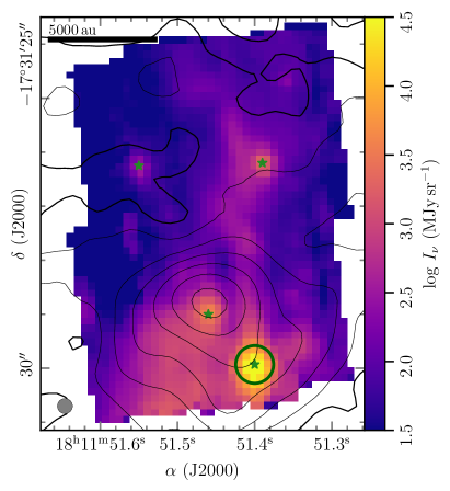
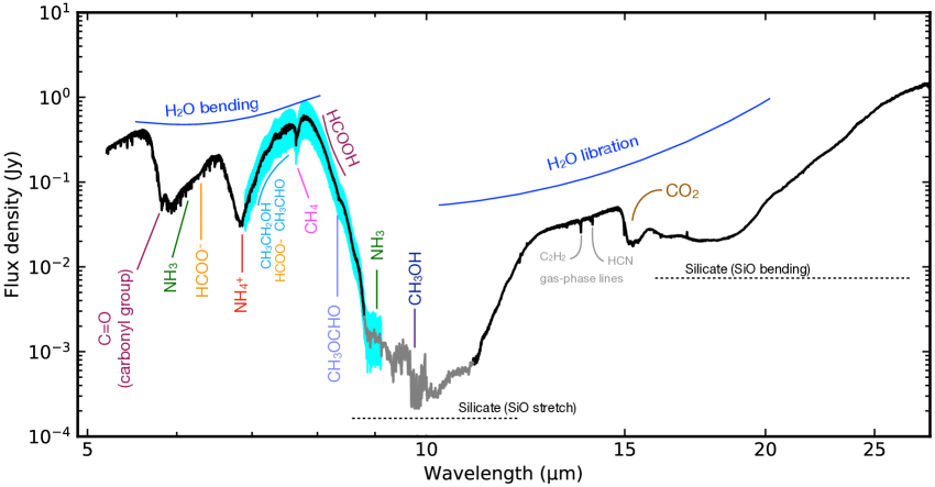
Figure 21: Left: MIRI-MRS 5 $\mu$m continuum image of the IRAS 18089-1732. The four compact sources are marked by green stars. The 0.7^′′ aperture used to extract the MIRI-MRS spectrum of the brightest mid-infrared source is indicated by the green circle. A scale bar of 5000 au is shown in the top and the angular resolution at 5 $\mu$m is shown in the bottom left corner. Black contours are the ALMA 3 mm continuum emission taken from Gieser et al. (2023a) with contour steps at 5, 10, 20, 40, 80, 160, 320$\times\sigma_{\mathrm{cont}}(\sigma_{\mathrm{cont}}$=0.057 mJy beam^-1). Right: MIRI-MRS spectrum of IRAS 18089-1732. The main absorption features are annotated in the figure. Gas-phase lines are not labelled, except in the case of C₂H₂ and HCN at 13.7 and 14.0 $\mu$m. The cyan region between 7 and 9 $\mu$m is the spectral window analyzed in this work. Because of the low $S/N$ in the deep silicate absorption, the data between 8.9 and 10 $\mu$m are binned by a factor of 5.

7 Cold envelope: ices

This section presents JOYS results on ices. As Figure 2 shows, ice features are prominently seen at 5–20 $\mu$m in MIRI-MRS spectra extracted from the bright mid-infrared continuum. Detected ices range from simple molecules like H₂O, CO₂ and CH₄ to CH₃OH as the most complex molecule identified pre-JWST (Boogert et al., 2015). Background information can be found in § 2.3.4 and § B.4.

7.1 Detection of complex molecules in ices

The high $S/N$ JWST spectra allow weaker features to be identified, especially in the 5–10 $\mu$m range where Spitzer only had $R=50-100$. One of the early highlights of JOYS is the detection of complex molecules other than CH₃OH in ices toward the low-mass protostars NGC 1333 IRAS2A and B1-c and the high-mass source IRAS 23385+6053 (Rocha et al., 2024; Chen et al., 2024). These features occur in the range between 6.9-9.0 $\mu$m, also known as the icy COMs fingerprint region (Schutte et al., 1999; Öberg et al., 2011). To investigate how similar these COMs features are between low- and high-mass protostars, we analyze here a second high-mass protostar, IRAS 18089-1732.

Figure 21 presents the spectrum of IRAS 18089 extracted from the peak mid-infrared continuum in a 0.7^′′ aperture (RA=18h11m51.40s Dec=-17d31m29.93s). This aperture is optimized for the 7–9 $\mu$m region and is taken to be small, also at longer wavelengths to avoid blending with another source. IRAS 18089 has a luminosity of $\sim 10^{4}$ L_⊙ and envelope mass of $\sim$1000 M_⊙ based on single-dish observations (Sridharan et al., 2002; Beuther et al., 2002; Urquhart et al., 2018), at an estimated distance of 2.34 kpc (Xu et al., 2011). The source is known to be rich in gas-phase complex organic molecules (COMs) (e.g., Beuther et al., 2004; Isokoski et al., 2013).

Rocha et al. (2024) and Chen et al. (2024) found signatures of several icy COMs in their analyzed sources, including CH₃CHO (acetaldehyde), CH₃CH₂OH (ethanol), CH₃OCHO (methylformate), and CH₃OCH₃ (dimethylether). In addition, ice features of CH₄, HCOOH (formic acid), SO₂ and the negative ions OCN^- (cyanate ion) and HCOO^- (formate ion) are found in the 7–9 $\mu$m range. Here, we adopt the same methodology as in Rocha et al. (2024) to execute the spectral fitting. The first step is to remove the continuum, the deep silicate feature and the H₂O 12 $\mu$m ice libration band, which is described in detail in the Appendix F. This procedure also provides the total H₂O ice column density, which is found to be $(2.8\pm 0.7)\times 10^{19}$ cm^-2.

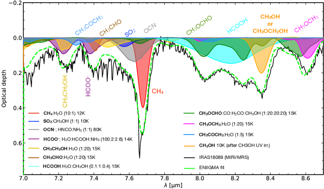
Figure 22: Spectral fit between 7 and 8.7 $\mu$m of IRAS 18089 using the ENIIGMA fitting tool with laboratory ice mixtures from the LIDA database. Eleven ice components are used to obtain the best fit, which includes simple and complex molecules in ice mixtures. The boldface in the labels of the lab spectra indicates the main species that contributes in this spectral range. The narrow weak absorption features between 7 and 8 $\mu$m are primarily due to warm gas-phase H₂O; the narrow peak at 7.66 $\mu$m is due to gaseous CH₄ absorption.

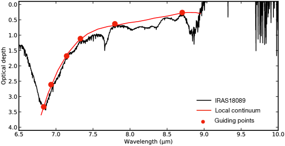
Figure 34: Local continuum fit and guiding points for the 7–9 $\mu$m range of the IRAS 18089 spectrum, after subtraction of the global continuum, silicate feature and water libration band.

The next step is to choose a local continuum for the 6.9–9.0 $\mu$m region on the optical depth spectrum that has been corrected for the global continuum, silicate feature and H₂O libration bands (see Fig. 33). This local continuum takes into account absorption features from major species in this interval, such as the H₂O ice 6 $\mu$m bending mode, the prominent NH${}_{4}^{+}$ 6.8 $\mu$m profile, and likely organic refractory material (Gibb et al., 2004). Figure 34 in Appendix F shows this local continuum profile, which is obtained by fitting a 5th-order polynomial to guiding points to avoid unrealistic inflections. Note that a small but important excess is left around 7 $\mu$m since the CH₃ bending mode of several COMs contributes to this range.

After this local continuum subtraction, the spectrum is fitted using the IR laboratory spectra of simple and complex molecules from the LIDA database, following Rocha et al. (2024) using the ENIIGMA fitting tool (Rocha et al., 2021). This code combines a large number of laboratory ice spectra in small groups of components aiming to find the best solution given by the $\chi^{2}$. Starting from all possible species, a solution was found for IRAS 18089 that combines 11 ice mixtures, containing absorption features in the fitted wavelength range of CH₄, SO₂, OCN^-, HCOO^-, CH₃CH₂OH, CH₃CHO, CH₃OCHO, HCOOH, CH₃OCH₃ and CH₃COCH₃ (acetone), as shown in Figure 22.

Based on the statistical methods and criteria of Rocha et al. (2024) and as embedded in the ENIIGMA code, most of these identifications are thought to be secure; acetone is considered tentative for the case of IRAS 18089 (but see also discussion in Chen et al. 2024 for B1-c). The presence of H₂CO is based only on its 8 $\mu$m band and would need to be confirmed at shorter wavelengths. Note that SO₂ ice is detected in this high-mass source, in contrast to the case of IRAS 23385 (Rocha et al., 2024). CH₃COOH (acetic acid) is not detected in either of the high-mass sources although its detection is sensitive to the local continuum placement at 7.8–8.0 $\mu$m.

Indeed, more generally, the detections and abundances of icy COMs remain sensitive to the details of the global and local continuum placement and subtraction. While the uncertainty in the global continuum reflects the source structure and spectral energy distribution, the local continuum must reflect the contribution of less understood species, such as salts and organic refractory materials that show broader infrared absorption features from 6 to 8 $\mu$m. Laboratory spectra are often available for only a limited range of ice mixtures and temperatures, although the current list already reflects huge experimental efforts focusing on those icy COMs that are also abundant in the gas-phase. Indeed, arguments in support of their identification include the detection of the same COMs at comparable abundances in the gas phase in the same source (see Chen et al., 2024; Nazari et al., 2024a, and below). New measurements to enlarge the icy COMs inventory in the laboratory exploring new ice mixtures in realistic abundances at a range of temperatures are encouraged, as well as more studies on the chemical composition of the organic refractory materials.

The IRAS 18089 spectrum contains a prominent 8.38 $\mu$m feature that has been seen in only few other JWST ice spectra analyzed so far (B1-c, L1527, IRAS2A). Possible identifications include the hydroxymethyl radical (CH₂OH) or methoxymethanol (CH₃OCH₂OH). It will be discussed in a future paper that will also include new laboratory spectroscopy.

The derived ice column densities for the species fitted in this work are presented in Table 6. Note that CH₃OH is extracted from the bottom of the silicate feature for IRAS 18089, since no NIRSpec data are available for this source. The adopted band strengths are listed in Table 1 of Rocha et al. (2024). Uncertainties in inferred column densities are included in the table and are typically $\sim$30%.

Figure 23 compares the ice columns w.r.t. that of H₂O for the high-mass sources IRAS 18089 and IRAS 23385 versus the low-mass sources IRAS2A and B1-c. Very similar patterns are seen: not only are the same molecules detected in all four sources, but their abundances w.r.t. H₂O are also found to be comparable within the uncertainties for many species. Comparing high- and low-mass protostars, interestingly, methyl formate (CH₃OCHO) seems to show larger variations from source to source.

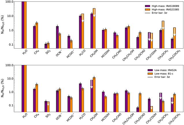
Figure 23: Comparison of ice abundances w.r.t. H₂O for the high-mass sources IRAS 18089 and IRAS 23385 (top) versus the low-mass protostars NGC 1333 IRAS2A and B1-c (bottom). White arrows indicate upper limits. The IRAS2A and IRAS 23385 results are taken from Rocha et al. (2024) and B1-c from Chen et al. (2024).

Chen et al. (2024) went one step further and compared the results for organic molecules in ices for the two low-mass protostars B1-c and NGC 1333 IRAS2A with those found in the gas phase in hot cores with ALMA toward the same sources. Interestingly, the ratios of some of the most abundant O-COMs with respect to methanol, CH₃OCHO/CH₃OH and CH₃OCH₃/CH₃OH, are very similar in ice and gas, supporting the picture of ice sublimation producing these species in their hot cores. However, the gaseous ratios of CH₃CHO/CH₃OH and C₂H₅OH/CH₃OH appear lower than those found in ices. Unless these COM ice abundances are overestimated, this suggests that some COMs may be destroyed quickly in the gas following sublimation (see discussion in Chen et al. 2024 and in Chen et al. 2025 for the case of acetone).

Besides quantification of ice column densities, comparisons between laboratory and observed infrared spectra also reveal information on ice temperatures and mixing conditions (i.e., mixing constituents and mixing ratios) of the detected COM ices, as these factors vary the peak position and the profile of their absorption bands. Rocha et al. (2024) and Chen et al. (2024) found that most of their detected COM ices are likely surrounded by a H₂O-rich environment, with CH₃OCHO as an outlier that is suggested to be present in a CO- and CH₃OH-rich layer. The inference on temperature is much more degenerate since many COM ice bands do not change much below their crystallization temperatures (usually $\sim$100 K in the laboratory, 20%—40% lower in space due to lower pressures). Investigation of a larger sample is needed to solidify these results.

7.2 Ammonium salts in ices

The fit to the 7–9 $\mu$m range of the four sources for which the COMs have been analyzed (Fig. 23) also indicate the presence of two negative ions in the ices: HCOO^- and OCN^- (see Fig. 22). The latter ion has been identified previously through its strong band at 4.62 $\mu$m seen along many lines of sight (e.g., Grim & Greenberg, 1987; Novozamsky et al., 2001; van Broekhuizen et al., 2004), now also with JWST-NIRSpec (McClure et al., 2023; Nazari et al., 2024a). Together with the positive ion NH${}_{4}^{+}$ that is ubiquitously detected at 6.85 $\mu$m (Fig. 2 and 21), they make up ammonium salts that are readily produced by acid-base reactions in ices (Knacke et al., 1982; Boogert et al., 2015, for review). Salts have recently gained renewed interest since they are found in high abundances in cometary material as one of the major nitrogen reservoirs (Altwegg et al., 2019) and also in the gas-phase in some high-mass protostars (Ginsburg et al., 2023).

The JWST JOYS analysis confirms the identification of the OCN^- ion through its bending mode at 7.6 $\mu$m and strengthens the assignment of the HCOO^- ion as significant contributors to the 7.2 and 7.4 $\mu$m absorption bands, suggested by Schutte et al. (1999); Schutte & Khanna (2003). Moreover, they indicate the presence of ammonium hydrosulfide NH₄SH as the dominant ammonium salt in ices with SH^- the main counterpart of NH${}_{4}^{+}$ and locking up 18–19 % of the sulfur in dense clouds (Slavicinska et al., 2025b); see Figure 35 for a fit to the 6.85 $\mu$m band of IRAS 18089. The ice anion abundances with respect to NH${}_{4}^{+}$ are similar to those in comet 67P, where NH₄SH is also the dominant ammonium salt (Altwegg et al., 2022). Together, the identified icy N-species NH${}_{4}^{+}$ and OCN^- make up 19% of the available N-budget (see Appendix F for details). NH₃ ice is difficult to measure in these data (Fig. 21), but, if its column were as high as 10% of H₂O ice (Boogert et al., 2015), it would increase the N–budget to 31%. Future studies using the larger JOYS+ sample and combining NIRSpec and MIRI will allow these ions to be studied across the Class 0 and I stages.

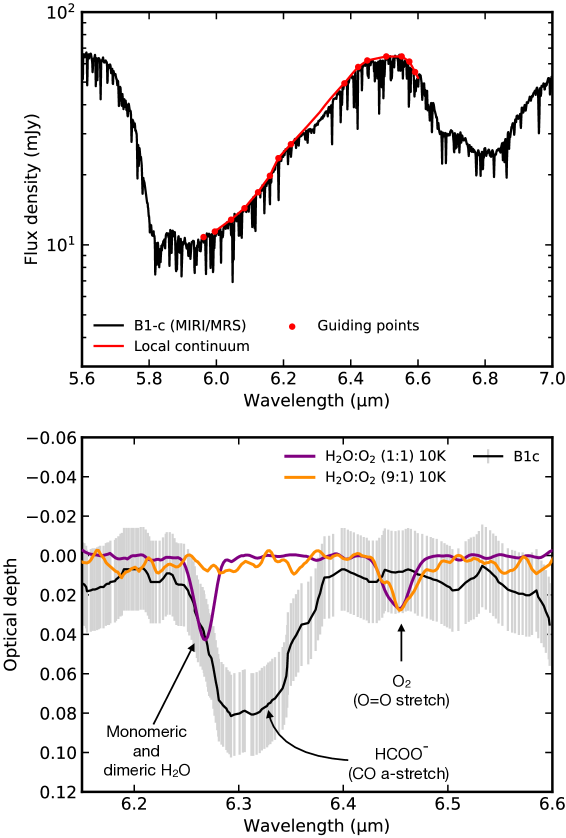
Figure 24: Limits on O₂ ice in the spectrum of the low-mass protostar B1-c. The top panel shows the local continuum used between 6 and 6.6 $\mu$m together with the anchor points. The narrow absorption lines are all due to gas-phase water absorption (van Gelder et al., 2024a). The bottom panel presents the optical depth spectrum with 3$\sigma$ error bars compared with O₂:H₂O ice laboratory spectra (Müller et al., 2018).

7.3 Limits on O₂ ice

H₂O is the most abundant molecule detected in ices but it contains only a moderate fraction of the total oxygen budget, typically $\lesssim 20\%$ (Whittet, 2010; van Dishoeck et al., 2021). A significant fraction of oxygen must therefore be in other forms, and O₂ has been suggested as an option, although observations to date indicate that it is not a major reservoir, neither in gas (Goldsmith et al., 2011; Liseau et al., 2012; Yıldız et al., 2013) nor in ice (Vandenbussche et al., 1999). See § B.4 for more background information.

New impetus for searching for interstellar O₂ ice has come from the detection of abundant O₂ ice in comet 67P by the ROSINA instrument on board of the Rosetta mission (Bieler et al., 2015; Rubin et al., 2019). The cometary O₂ abundance is found to follow closely that of H₂O with heliocentric distance at a mean ratio of O₂/H₂O$\approx$0.03. While not a major oxygen reservoir, this still makes O₂ a significant ice component. Moreover, it provides insight into the major oxygen chemistry pathways: producing O₂ ice at this level through gas-grain chemistry requires special conditions (high density, low cosmic ray ionization rate) in the pre-stellar cloud to suppress water ice formation (Taquet et al., 2016).

Since O₂ is infrared inactive, it does not have a strong ice band in its pure ice form. However, if mixed with H₂O ice as suggested by the cometary results, its 6.45 $\mu$m band becomes weakly visible (Ehrenfreund et al., 1992; Müller et al., 2018). ISO-SWS was able to put only weak limits on the 6.45 $\mu$m feature in a few warm high-mass sources due to its low $S/N\approx 10$ on the continuum (Vandenbussche et al., 1999).

Here we use the deep MIRI spectrum of the most ice-rich source in the JOYS sample, the low-mass Class 0 source B1-c, to search for solid O₂. With an integration time of 1800 sec in Channel 1C, this spectrum achieves a $S/N>100$ on the continuum (Fig. 2). The data reduction details can be found in Chen et al. (2024). Figure 24 presents a blow up of the B1-c MIRI-MRS spectrum extracted at the source position in the 6–7 $\mu$m range. This region is dominated by the deep H₂O ice bending mode absorption at 6.0 $\mu$m with NH₃ ice at 6.18 $\mu$m, and the deep NH${}_{4}^{+}$ band at 6.8 $\mu$m. Moreover, the B1-c spectrum is rich in narrow gas-phase absorption lines, most of them due to warm H₂O vapor that are superposed on the ice features (van Gelder et al., 2024a). A local continuum subtraction is performed between 6 and 6.6 $\mu$m, where any contribution of O₂ ice is expected (Fig. 24, top). Some anchor points are used in this fit to leave some space for known absorption features and ensure smooth curvature, and a 5th-order polynomial is then adopted to trace the continuum.

Subtracting all of these features and overlaying laboratory spectra of various O₂:H₂O mixtures provides a $3\sigma$ limit of O₂ (Fig. 24, bottom). The inferred value is $N_{s}$(O₂)$<4.9\times 10^{18}$ cm^-2, using a band strength $A=3.9\times 10^{-20}$ cm molecule^-1 appropriate for 1:1 O₂ ice mixtures with H₂O (Müller et al., 2018). Together with $N_{s}$(H₂O)=$2.5\times 10^{19}$ cm^-2 (Chen et al., 2024), this provides an O₂ limit of $\sim$20% w.r.t. H₂O ice. Due to the strong dependence of the band strength on H₂O ice concentration, this value may be increased by a factor of 5. Note that layered ice models indicate that O₂ is not uniformly mixed with H₂O ice (see Figure 5 in Taquet et al., 2016), hence the use of an O₂:H₂O laboratory spectrum with a lower mixture than 1:30 could be justified. Nevertheless, it is clear that even with the sensitivity of JWST, it is not possible to put stringent limits on the O₂ ice abundance (Müller et al., 2018) and test values of order 3% as found in cometary ices.

Future indirect constraints on the O₂ ice abundance may come from the analysis of the ¹³CO ice profile at 4.8 $\mu$m and from searches for photoproducts of O₂ ice such as O₃ and CO₃ ice using both NIRSpec and MIRI data (Ehrenfreund & van Dishoeck, 1998; Vandenbussche et al., 1999; Pontoppidan et al., 2003).

7.4 HDO/H₂O in protostellar ices

While there have been multiple determinations of the gaseous HDO/H₂O ratio in hot cores (Persson et al., 2014; Jensen et al., 2019), its value in interstellar ices remained poorly constrained prior to JWST (Dartois et al., 2003; Aikawa et al., 2012). JWST-NIRSpec offers the opportunity for deep searches for HDO ice through its O-D stretching mode at $\sim$4.1 $\mu$m. Searches for this feature are complicated by the nearby weak CH₃OH 3.8–3.9 $\mu$m combination mode (Dartois et al., 2003), and a potential S-H stretch from molecules like H₂S or SH^- at 3.9 $\mu$m. On the other side of the HDO ice band, the deep ¹²CO₂ 4.3 $\mu$m ice absorption can distort the local continuum due to scattered light off ices, a process that is sensitive to grain shape effects (Dartois et al., 2022).

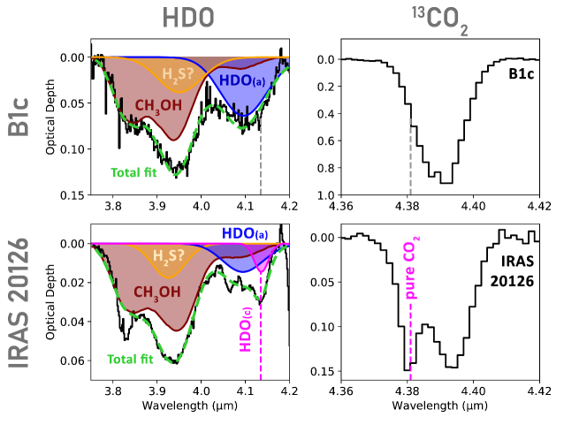
Figure 25: Top panel, left: JWST NIRSpec spectrum of B1-c in the 3.8–4.2 $\mu$m range, highlighting the detection of HDO ice. Laboratory spectra of HDO amorphous ice (HDO(a)) as well as of CH₃OH ice are overlaid. A Gaussian has been added to represent an S-H ice feature. The top right panel shows the ¹³CO₂ 4.38 $\mu$m ice band of B1-c, highlighting the lack of a heated ice component. Bottom panel, left: JWST NIRSpec spectrum of the high mass protostar IRAS 20126 taken from Slavicinska et al. (2024) showing the detection of both amorphous and crystalline HDO ice. The laboratory spectrum of crystalline HDO ice is shown in pink (HDO(c)). The bottom right panel shows that the ¹³CO₂ 4.38 $\mu$m ice band of IRAS 20126 indeed shows evidence of a heated ice component as analyzed by Brunken et al. (2024a).

Slavicinska et al. (2024) recently presented the first robust detections of crystalline and amorphous HDO ice toward the intermediate- and high-mass protostars HOPS 370 (310 L_⊙) and IRAS 20126 ($10^{4}$ L_⊙) as part of the IPA sample. A careful decomposition of the 3.8–4.2 $\mu$m ice band was performed, using new laboratory data and obtaining a consistent fit with the CH₃OH 3.54 $\mu$m band to assess the contribution of CH₃OH ice at 3.8–3.9 $\mu$m. Both crystalline and amorphous HDO ice were required to fit the feature, consistent with the fact that both are warm sources as deduced also from the shape of their 3 $\mu$m H₂O ice bands showing crystalline H₂O ice and the analysis of their ¹³CO₂ 4.38 $\mu$m bands (Brunken et al., 2024a). Both the HDO and ¹³CO₂ spectra for IRAS 20126 are included in Figure 25 (bottom). The inferred HDO/H₂O ice ratios range from $(3-5)\times 10^{-3}$, comparable with the highest reported warm gaseous HDO/H₂O ratios in high-mass hot cores where ices have thermally sublimated.

The most prominent HDO ice detection to date is that toward the low mass Class 0 protostar L1527 using the G395M NIRSpec spectrum from program 1798 (PI: J. Tobin), which shows a significantly deeper deuterated water ice feature (Slavicinska et al., 2025a). This detection is particularly exciting, since this low-mass source provides a window into what the HDO/H₂O ice ratio in our own protosolar system could have been. The inferred value of $4.8\times 10^{-3}$ with an uncertainty of $\sim$60% is at the upper end of the gaseous HDO/H₂O ratios in other isolated low-mass protostars (Jensen et al., 2019).

To explore whether the HDO/H₂O ice ratio toward L1527 is representative for solar-mass systems, we present here a second detection of HDO ice toward a low-mass protostar, B1-c. A NIRSpec G395M $R\sim 1000$ spectrum was taken as part of JOYS (program 1290). Note that all other NIRSpec spectra in JOYS+ used the G395H $R\sim 2700$ mode which has a gap precisely at 4.1 $\mu$m and can therefore not be used for HDO searches. Within the JOYS+ data set, the low resolution PRISM mode could still be used for that purpose, albeit with less fidelity at $R$ of only $\sim$200. Such a PRISM study will be left for a future paper.

Figure 25 (top) presents a blow-up of the 3.8–4.2 $\mu$m spectrum for B1-c over the same region as shown in Slavicinska et al. (2024, 2025a) for the other sources. One complication for B1-c is that the blue side of the deep CO₂ ice feature shows clear signs of grain growth which affects the continuum determination. This wing has been removed using a local continuum in a similar manner as for L1527. Once removed, a clear HDO + CH₃OH feature emerges. Using the same fitting procedure as in Slavicinska et al. (2024, 2025a), an HDO column of $1.2\times 10^{17}$ cm^-2 is derived. The H₂O 3 $\mu$m band is completely saturated and below the noise in this source but an H₂O column density of $2.5\times 10^{19}$ cm^-2 has been derived by Chen et al. (2024) from the H₂O libration mode (see also above section on O₂ ice limits for B1-c). Together this gives HDO/H₂O=$(4.8\pm 3.0)\times 10^{-3}$, consistent with that found toward L1527. As for L1527, the uncertainties are dominated by the placement of the continuum and variations in band strength with temperature (see discussion in Slavicinska et al. 2025a).

Both values are close to that recently found in warm gas in a young protoplanetary disk where ice has sublimated (Tobin et al., 2023) (see Fig. 4 in Slavicinska et al. (2025a)). They are somewhat higher than those measured in comets in our Solar system, suggesting that even though a large fraction of the water ice appears to be largely preserved in its journey from clouds to disks (Visser et al., 2009; Cleeves et al., 2014; van Dishoeck et al., 2021), some modifications may occur along the way to the comet and planetesimal formation sites (Furuya et al., 2017).

The HDO fit for B1-c requires only the presence of amorphous HDO ice. Since the H₂O 3 $\mu$m band profile cannot be observed in B1-c and the 12 $\mu$m band does not have a distinct crystalline feature, it is not possible to check whether there is any crystalline H₂O ice. However, the lack of crystalline HDO ice is consistent with the fact that the ¹³CO₂ ice band, included in Figure 25 (top), has only a single broad feature that can be fitted with cold CO₂:H₂O or CO₂:CH₃OH ice mixtures: no separate narrow blue-shifted peak due to heated pure CO₂ ice is needed as found for other sources (Brunken et al., 2024a). Similarly, the deep CO₂ 15 $\mu$m bending mode of B1-c (Fig. 2) shows no hint of a double-peaked structure that is characteristic of heated ices. This suggests that, in contrast with the other sources, B1-c has not undergone episodes of intense accretion activity in the past that were strong enough to crystallize a significant portion of the ices: once crystallized, the process is irreversible.

8 Embedded disks

Disks are an integral part of protostellar systems, but little is still known about their composition in the embedded stage. A related question is to what extent these young disks are affected by accretion shocks of material falling onto the disk. Background information on this science case can be found in § 2.3 and § B.5.

8.1 Low-mass protostars

8.1.1 JWST spectra of sources with embedded disks

JWST MIRI-MRS data show rich spectra of Class II disks around pre-main sequence stars pointing to a diverse chemistry in their inner few au (see § B.5). Some disks are very rich in H₂O (e.g., Gasman et al., 2023; Temmink et al., 2024a; Romero-Mirza et al., 2024; Banzatti et al., 2025), some are less H₂O rich (e.g., Perotti et al., 2023), whereas other disks show a prominent ⁽¹³⁾CO₂ feature (e.g., Grant et al., 2023; Vlasblom et al., 2025). Disks around very low mass stars often have strong emission from hydrocarbon molecules with only weak water lines (e.g., Tabone et al., 2023; Arabhavi et al., 2024, 2025; Kanwar et al., 2024). Excitation temperatures are high, from $\sim$300 K up to 900 K. This diversity is thought to be linked to icy pebbles drifting from the outer to the inner disk, thereby enhancing molecules like H₂O and CO₂ when they cross their snowlines on timescales of 1-2 Myr. Dust traps locking up volatile elements in ices in the outer disks achieve the opposite effect of lowering their abundances (Kalyaan et al., 2023; Mah et al., 2023, 2024; Sellek et al., 2025).

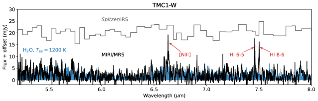
Figure 26: JWST MIRI-MRS spectrum of the Class I TMC1-W source showing a forest of hot H₂O water lines. A LTE slab model at 1200 K is included for comparison in blue. The Spitzer-IRS spectrum of the binary TMC1 source is shown for comparison, illustrating that these types of detections were not possible prior to JWST. Figure adapted from van Gelder et al. (2024a), which shows the model spectrum offset from the data.

Since disks already form early in the Class 0 phase and are well established by the Class I phase (e.g., Ohashi et al., 2023; Tobin & Sheehan, 2024), a prime question concerns the chemical composition of the inner regions of embedded young disks, at a time of $<0.5$ Myr when they are still pristine and not yet affected by radial drift of icy grains from the outer disk and/or when dust traps have not yet developed to interrupt the pebble flux.

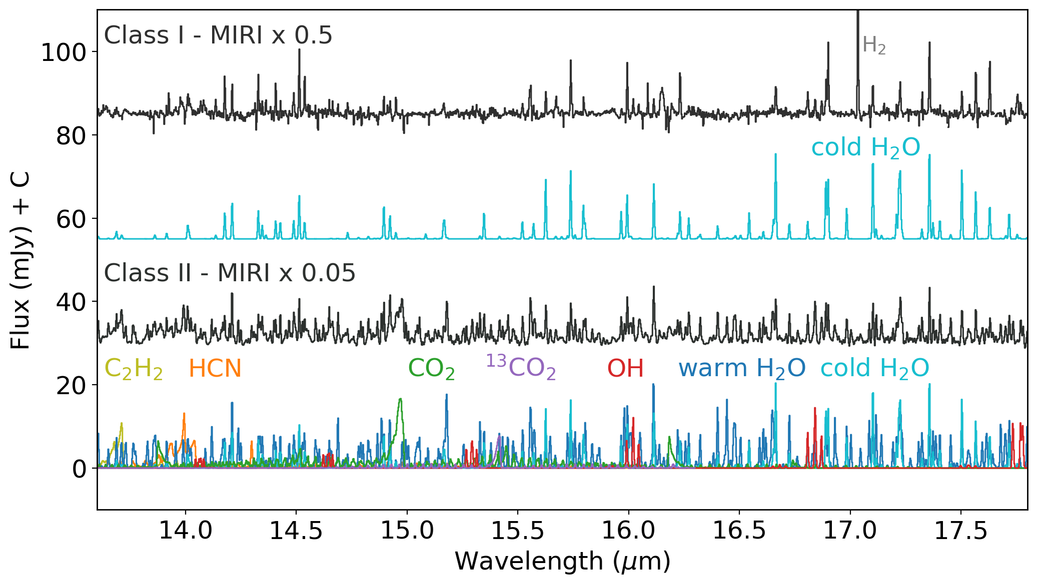
Figure 27: MIRI-MRS spectra at 13.5–17.5 $\mu$m of the Class I source B1-a-NS showing only cold water (van Gelder et al., 2024a), and the Class II disk DF Tau being rich in warm H₂O and other molecules (Grant et al., 2024). The colored spectra show LTE slab models of individual molecules contributing to the observed spectra; they are meant to illustrate the positions of the lines, not as a fit to the data. The temperatures used on the H₂O slab models are 190 K (cold) and 490 K (warm)

Class I disks should have warm gas in their inner regions, just as Class II disks. Indeed, evidence for the presence of warm disk gas down to $\sim$0.1 au is provided by VLT-CRIRES ¹²CO $v$=2–1 infrared line emission profiles at 4.6 $\mu$m (Herczeg et al., 2011). It therefore came as a surprise that the molecular line survey of the JOYS sources by van Gelder et al. (2024a) found primarily low excitation temperatures, not at all characteristic of inner disks (§ 6). Only one source with hot H₂O was uncovered, TMC1-W, which is part of the $\sim$100 au separation binary source TMC1 with both sources showing evidence for a disk in millimeter continuum and line emission (Harsono et al., 2014; Tychoniec et al., 2021, 2024). Figure 26 presents the MIRI-MRS spectrum of the 5–8 $\mu$m range of this Class I protostar with the hot ($\sim$1200 K) water model overlaid. At first glance, the MIRI spectrum looks like pure noise, but blow-ups reveal that this is actually a forest of hot water lines (see also van Gelder et al., 2024a). Figure 26 includes the Spitzer-IRS spectrum for comparison to illustrate that such detections were not possible prior to JWST.

Figure 27 presents the 13.5–17.5 $\mu$m MIRI-MRS spectrum of one other Class I JOYS source, B1-a-NS. For comparison, the line-rich Class II disk DF Tau is shown, taken from Grant et al. (2024). This wavelength range contains several key molecules that are readily detected in Class II disks due to their $Q-$branches: CO₂, HCN and C₂H₂, in addition to the pure rotational lines of H₂O. It is clear that these Class I and II sources are very different, with B1-a showing only cold H₂O that is not even necessarily coming from the inner disk.

Figures 15 and 17 include the spectrum of our example source, the Class 0 protostar Serpens SMM3, which also shows evidence for a large embedded disk both in ALMA continuum and CO lines (Tychoniec et al., 2021) (Fig. 8). Like B1-a-NS, SMM3 shows no hints for warm molecular emission in the 13.5–17.5 $\mu$m range except for CO₂, nor at 22–26 $\mu$m for cold H₂O emission. The CO₂ emission appears extended along the outflow (Fig. 16), and may therefore not be arising from the inner disk. This example illustrates the importance of having spatial information at 30 au scales, as offered by MIRI-MRS.

8.1.2 Hiding warm molecular emission in young disks?

What could be the reason for the absence of warm molecular emission when a disk is clearly established? Figure 28 illustrates some differences between Class I and II disks. Some Class II disks also lack warm molecular emission, and in those cases the presence of a large inner cavity has been suggested (Banzatti et al., 2017; Vlasblom et al., 2024). Another related possibility is that dust traps in the outer disk have locked up water and other volatiles as ices, preventing the drifting icy pebbles from reaching the inner disk (e.g., Najita et al., 2013; Banzatti et al., 2020). However, the ALMA observations of a sample of representative Class 0 and I disks, including TMC1A, show little evidence for dust traps down to 5 au resolution (Ohashi et al., 2023). Also, even for Class II disks, gaps do not fully prevent oxygen and water from getting to the inner disk (e.g., Perotti et al., 2023; Schwarz et al., 2024; Gasman et al., 2025).

A more likely explanation is that the inner disk emission is hidden by small dust grains high up in the disk atmosphere, in any disk wind, and in the surrounding envelope. In Class II disks, the grains have grown and settled to the midplane, as evidenced by the fact that the analysis of their molecular emission generally invokes gas/(small) dust ratios of 10000 rather than 100 in the line emitting region to explain the line strengths and line/continuum ratios (e.g., Meijerink et al., 2009; Bruderer et al., 2015; Woitke et al., 2018; Greenwood et al., 2019; Bosman et al., 2022). Figure 11 of Vlasblom et al. (2024) presents a series of thermochemical disk model spectra of H₂O and CO₂ in the 13–17 $\mu$m range for gas/dust ratios of 100, 1000 and 10000 respectively, illustrating that the molecular emission is weakened by more than an order of magnitude at normal gas/dust ratios of 100. ALMA observations show clear evidence for highly settled large dust grains in the outer regions of Class II disks (e.g., Villenave et al., 2020), but much less in Class I disks (Villenave et al., 2023).

Assuming ISM dust-to-gas ratios, the time taken for dust grains to grow large enough to settle is of the order of 1000 orbits at any given radius, which is $\sim$100 kyr for the outer disk. Drift thus likely begins sometime early on in the Class I phase. However, due to (i) the initial enrichment of the inner disk with dust from the outer disk, (ii) the timescale (100s of orbits) for the large grains to settle and drift, and (iii) the resupply of dust from the envelope, the dust-to-gas ratio can remain high up to $\sim$0.3–0.4 Myr (e.g., Cridland et al., 2022; Appelgren et al., 2023), i.e., for most of the Class I phase, likely even in the upper layers. Thus the levels of dust depletion needed to reproduce the line strengths in Class II disks are likely not achievable during the Class I phase even if drift is active to supply volatiles. Indeed, models of drifting icy grains find that inner disks are not only enhanced in H₂O but also in small dust that may mask the molecular features (Sellek et al., 2025; Houge et al., 2025).

While dust extinction could be an explanation for these MIRI observations, it remains puzzling that CO infrared disk emission, which should be similarly affected by dust extinction, is seen for several Class I sources (Herczeg et al., 2011), including TMC1A and TMC1 that are part of JOYS. Likely this CO emission, in particular that from overtone bands, arises from the dust-free inner disk gas (Bosman et al., 2019; Banzatti et al., 2022), as has been found from spatially resolved near-IR VLTI-Gravity observations of disks around more massive stars (e.g., GRAVITY Collaboration et al., 2021). Also, at least for the TMC1A disk, grain growth, and thus likely settling, has been inferred (Harsono et al., 2018).

Disk wind absorption superposed on disk emission is another option to minimize the molecular lines at the limited MIRI-MRS spectral resolution (Herczeg et al., 2011): high spectral resolution ($R\sim 100000$) VLT-CRIRES data reveal the presence of strong blue-shifted disk winds in absorption in ¹²CO $v=$1–0 and ¹³CO $v$=1–0 line profiles for many Class I sources. At MIRI-MRS spectral resolution, the emission and absorption may well cancel out (see also Banzatti et al., 2022). Such superposed absorption would be particularly important for bands that connect to the vibrational ground state. However it should not affect the highly excited pure rotational H₂O lines. Also, no C₂H₂ or HCN has yet been found associated with winds (see § 6.4), except perhaps in the case of Oph IRS 46 (Lahuis et al., 2006). Further observations and analysis of a much larger sample of low-mass Class I disks, offered partially by JOYS+ and by approved Cycle 4 programs, is needed to determine whether the lack of warm molecular emission from embedded disks is found more commonly.

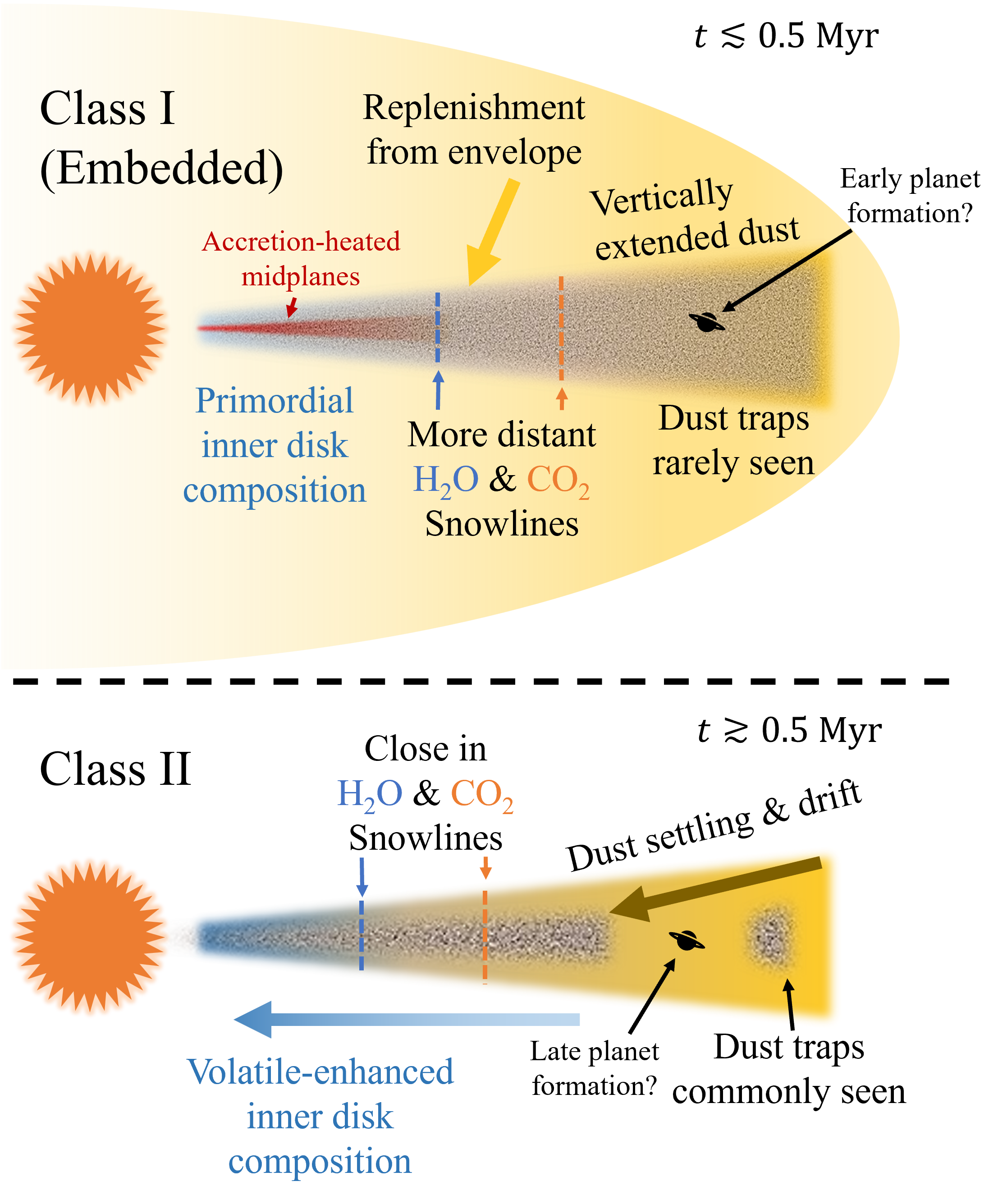
Figure 28: Cartoon illustrating differences in the physical and chemical structures of young Class I ($\sim$0.5 Myr) (top) and more mature Class II ($\sim$3 Myr) (bottom) disks.

8.1.3 Evidence for accretion shocks?

A final question is whether the JWST data provide any indication of accretion shocks triggered by infall or streamers onto the disk. ALMA observations have suggested that sulfur-bearing molecules, most notably SO and SO₂, are good tracers of such shocks (Sakai et al., 2014; Artur de la Villarmois et al., 2019; Liu et al., 2025). JWST MIRI has detected SO₂ ro-vibrational emission at 7.3 $\mu$m for the first time on disk scales of a Class 0 source, but comparison with ALMA data suggests that a hot core rather than accretion shock origin is more likely. Also, SO₂ infrared emission is not commonly seen (van Gelder et al., 2024a). The use of [S I] 25 $\mu$m emission as an accretion shock tracer warrants further investigation, especially in Class I sources where it is not associated with the outflow, but is limited by the low spatial resolution in Channel 4. Searching for local H₂ emission hot spots near the disk surface is another option.

8.2 High-mass protostars

Several high-mass protostars have been found to have Keplerian disks based on high-resolution ALMA data (see § B.5), including IRAS 18089 (Beuther et al., 2007), although this has not yet been established for all high-mass sources included in JOYS. Due to their higher accretion rates and luminosities, the midplanes of disks around high-mass protostars can be heated to much higher temperatures than the upper disk layers resulting in a temperature gradient that is decreasing rather than increasing with height (D’Alessio et al., 1997; Harsono et al., 2015; Nazari et al., 2023). Barr et al. (2020) have proposed that the warm H₂O absorption at 7 $\mu$m seen at high spectral resolution data with SOFIA-EXES and ground-based instruments toward high-mass protostars actually arises in the accretion-heated inner midplane of disks. The warm H₂O absorption seen with MIRI-MRS toward IRAS 23385 (Francis et al., 2024) and IRAS 18089 (Figures. 21 and 22) hints that this scenario could also hold for other high-mass protostars. Inspired by this scenario and using a radiative transfer model of Nazari et al. (2023) to characterize the temperature structure of an accreting massive disk, van Dishoeck et al. (2023) suggest that the cool CO₂ 15 $\mu$m emission observed toward IRAS 23385 (Fig. 20) could arise from the colder surface layers of the outer disk around one or both of the protostars. Alternative hot core and outflow scenarios such as discussed in § 6 cannot be excluded, however. Combined JWST, ALMA and high-resolution ground-based data are needed to disentangle the origin of the mid-infrared emission or absorption. Because of the high extinction, a pole-on geometry would be more favorable to peer into the inner disk-like structures. If a disk origin can be established, it would provide a unique probe of the physical and chemical structure of inner disks of high-mass protostars.

9 Conclusions

JWST’s exquisite sensitivity combined with the much higher spectral and spatial resolution offered by the MIRI-MRS IFU allow a new view of low- and high-mass protostars in their most deeply embedded stages. This paper presents a scala of illustrative results on a sample of 23 low- + high-mass targets (32 if binaries are included) addressing their physical and chemical evolution. A summary of published JOYS and JOYS+ studies to date is listed in § B.6.

Our main findings are as follows:

1. Mid-IR H I recombination lines, in particular the H I 7–6 Humphreys $\alpha$ line at 12.37 $\mu$m, provide a powerful tool to measure accretion rates onto protostars in the earliest highly extincted stages. Inferred accretion rates for low-mass sources show a wide range of values, suggesting some sources to be in a low accretion, quiescent stage. Analysis of one high-mass source indicates accretion rates that are high enough to form high-mass stars.

2. Jets commonly show a nested physical structure with an ionized core traced best by [Fe II] emission, surrounded by a molecular layer traced by the higher-$J$ H₂ pure rotational lines. This structure is seen across the entire protostellar mass range. For some low-mass sources, the molecular gas provides the main thrust in the earliest Class 0 stages, but this phase appears to be short lived. By the Class I stage, the outflows become fully atomic and ionized. The need for high resolution data to determine mass loss rates is emphasized.

3. Wide-angle winds traced by the lower-$J$ pure-rotational H₂ lines are commonly found inside the outflow cavity walls, that can be outlined by scattered light and by entrained cold gas in CO millimeter lines. Their temperatures of a few hundred to 2000 K are lower than those of the jets, with gradients seen perpendicular to the jet axis. The main heating mechanisms of the gas may vary from position to position and warrant further investigation.

4. A large variety of atomic and ionic lines from refractory, semi-refractory and volatile elements have been detected and imaged in most sources, showing different morphologies that are related to different levels of elemental depletions, local shock conditions and, in the case of noble gases, photoionization. Also, 20 $\mu$m continuum emission due to heated dust has been found in a few very young Class 0 sources. Together with the atomic lines, this allows questions of dust launching in jets and grain destruction in shocks to be quantified.

5. Hot core and dense shock chemistry models can be tested with unprecedented detail through observations of simple key molecules like H₂O, CO₂, HCN, C₂H₂, OH, and SO₂ in both low- and high-mass sources. Derivation of their abundances requires use of non-LTE excitation models including infrared pumping. Ice sublimation followed by high-temperature gas phase chemistry, perhaps stimulated by X-rays, explains the data for some sources, whereas dense jet shocks are more appropriate for others. No clear indication for accretion shocks onto low-mass disks has yet been found. The case of NGC 1333 IRAS4B provides a unique data set to test dense shock chemistry models, including the chemical processes that lead to bright hot C₂H₂ emission.

6. Ice studies have made a significant jump thanks to the high-quality MIRI-MRS data in the 5–10 $\mu$m range. Several complex organic molecules and ions (salts) have been found with comparable abundances in low- and high-mass protostars. The second detection of HDO ice in a low-mass protostar is reported here, with HDO/H₂O ice ratios that point to inheritance from cloud to disk. O₂ ice remains elusive, with JWST providing improved limits.

7. Young disks in the embedded stage do not show the same forest of warm molecular lines as more evolved Class II disks do. A likely explanation is that small dust has not yet grown and settled and is being replenished by radial drift, thereby obscuring a clear view to their inner few au. Extinction from dust in a disk wind or envelope may also contribute.

This paper provides a first comprehensive look into JWST MIRI-MRS studies of a significant sample of protostars. So far, many similarities between low- and high-mass sources are found. Larger samples across evolutionary stages and stellar mass range, such as offered by JOYS+ and by other currently ongoing and future programs like HEFE (High angular-resolution observations of Emergence in Filamentary Environments, P.I. T. Megeath), will allow much more robust trends to be identified. In particular, the low-mass sample in JOYS contains only 4 (6 with binaries) Class I sources and will be more than doubled in JOYS+. HEFE will add many more Class 0 sources of intermediate luminosity in a highly irradiated environment. Such large samples will also help in interpreting similar spectra seen in extragalactic sources.

More robust calibrations of mass loss and mass accretion rates need to be developed and quantified. Studies of binaries/clustering will be possible at 0.5–5^′′ separation with the JOYS+ sample. The combined NIRSpec + MIRI study will increase the available diagnostics, including higher excitation [Fe II] and H₂ lines that probe hotter gas. The results from such studies ultimately need to be made consistent with the physical components of warm and hot gas found in CO and H₂O data with Herschel. The high spatial and spectral resolution of NIRSpec also allows key ices to be detected and ice mapping against the scattered light continuum to be conducted. NIRCam imaging and spectral mapping can do so as well. When combined with ALMA and other instruments, JWST will truly help lifting the veil of key components of the youngest stages of stellar and planetary birth.

Appendix A Source positions

Table 1 contains the coordinates and properties of the JOYS sources. See also Table A.1 in van Gelder et al. (2024a) for more information on low-mass sources. Table 4 contains more information on the observational set-up.

Table 4: Main MIRI-MRS observational details of the sample of JOYS sources in the PID 1290 JWST GTO program.

ID	Archive name	Sources	RA	Dec	Dith	Exposure time	Background	Mosaic
			J2000	J2000		(s)
1	B1b-S	-	03:33:17.953	+31:09:31.49	2	1005, 1005, 1005	-	1$\times$1
2	B1b	B1-b	03:33:20.341	+31:07:21.36	2	200, 200, 200	B1b-S	1$\times$1
3	B1c-1	B1-c	03:33:17.953	+31:09:31.49	4	2009, 4029, 2009	B1b-S	1$\times$1
4	B1c-2	-	03:33:18.211	+31:09:28.63	2	200, 200, 200	B1b-S	1$\times$1
5	B1a	B1-a-1, 2	03:33:16.669	+31:07:54.90	2	200, 200, 200	B1b-S	1$\times$1
6	IRAS4B	IRAS4B	03:29:12.012	+31:13:07.07	2	200, 200, 200	B1b-S	1$\times$1
7	IRAS4B-b1	-	03:29:12.040	+31:13:01.35	2	200, 200, 200	B1b-S	1$\times$1
8	IRAS4A-b1	-	03:29:10.595	+31:13:19.40	2	200, 200, 200	B1b-S	1$\times$1
9	L1448mm	L1448-mm	03:25:38.761	+30:44:08.16	2	200, 200, 200	B1b-S	2$\times$3
10	Emb-8	Per-emb 8	03:44:43.982	+32:01:35.21	2	200, 200, 200	B1b-S	1$\times$1
11	Dark-Taurus	-	04:39:32.290	+26:05:14.50	1	200, 200, 200	-	1$\times$1
12	L1527-1	L1527 IRS	04:39:53.955	+26:03:09.56	2	1000, 1000, 1000	Dark-Taurus	1$\times$1
13	L1527-2	-	04:39:54.245	+26:03:11.67	2	200, 200, 200	Dark-Taurus	1$\times$1
14	TMC1A	TMC1-A	04:39:35.203	+25:41:45.17	2	216, 216, 216	Dark-Taurus	1$\times$1
15	TMC1	TMC1-W,E	04:41:12.700	+25:46:34.80	2	200, 200, 200	Dark-Taurus	1$\times$1
16	Dark-Serpens	-	18:29:48.250	+01:14:26.20	2	200, 200, 200	-	1$\times$1
17	SVS4-5	SVS 4-5	18:29:57.630	+01:13:00.20	2	605, 605, 605	Dark-Serpens	1$\times$1
18	SerpSMM3	Ser-SMM3	18:29:59.302	+01:14:00.97	2	200, 200, 200	Dark-Serpens	1$\times$1
19	SerpEmb8N	-	18:29:49.269	+01:16:52.62	2	200, 200, 200	Dark-Serpens	1$\times$1
20	SerpS68N	Ser-S68N-N, S	18:29:48.074	+01:16:43.80	2	200, 200, 200	Dark-Serpens	1$\times$1
21	SerpSMM1-2	Ser-SMM1-b1, b2	18:29:49.602	+01:15:21.90	2	200, 200, 200	Dark-Serpens	1$\times$1
22	SerpSMM1-1	Ser-SMM1-a	18:29:49.874	+01:15:19.79	4	200, 200, 200	Dark-Serpens	1$\times$1
23	Dark-BHR71	-	12:01:30:720	-65:08:44.60	2	200, 200, 200	-	1$\times$1
24	BHR71-IRS2	BHR71-IRS2	12:01:34.000	-65:08:47.00	2	200, 200, 200	Dark-BHR71	1$\times$1
25	BHR71-IRS1	BHR71-IRS1	12:01:36.548	-65:08:53.59	2	200, 200, 200	Dark-BHR71	3$\times$3
26	G28IRS2	G28IRS2	18:42:51.967	-3:59:53.985	2	200, 200, 200	-	1$\times$1
27	G28P1	A, B	18:42:50.679	-4:03:14.087	2	799, 799, 799	-	2$\times$2
28	G28S	-	18:42:46.414	-4:04:15.404	2	200, 200, 200	-	1$\times$1
29	Dark-IRAS23385	-	23:41:11.033	61:10:28.928	2	200, 200, 200	-	1$\times$1
30	IRAS23385	A, B	23:40:54.503	61:10:27.846	2	800, 800, 800	Dark-IRAS23385	2$\times$2
31	Dark-IRAS18089	-	18:11:44.112	-17:31:03.047	2	200, 200, 200	-	1$\times$1
32	IRAS18089	A, B, C	18:11:51.447	-17:31:27.285	2	400, 400, 400	Dark-IRAS18089	2$\times$1
33	Dark-G31	-	18:47:32.382	-1:13:44.317	2	200, 200, 200	-	1$\times$1
34	G31	G31	18:47:34.308	-1:12:46.000	2	200, 200, 200	Dark-G31	1$\times$1

Appendix B Scientific background

This section presents background information on the science cases addressed in this paper as well as the motivation for using JWST-MIRI in more detail than described in § 2.3. To avoid interrupting the flow of the results in Sections 4–8, this information is contained here in a single section. See also § 2 for terminology.

B.1 Protostellar accretion

Most of the protostellar accretion occurs in the earliest, deeply embedded stages (e.g., Lada & Wilking 1984; Hartmann et al. 2016) but there are very few direct measurements of the rates at which this process occurs. The H I recombination lines are thought to be good tracers if they are produced primarily in the accretion column onto the forming star. Most notably, the H I 7–6 Humphries $\alpha$ line at 12.37 $\mu$m has been proposed as an accretion tracer for highly extincted sources for which more commonly used shorter wavelength tracers like Brackett $\gamma$ cannot be observed (Rigliaco et al. 2015). However, H I recombination lines may also be produced in jet/wind shocks or circumstellar photoionized gas. The high spatial resolution imaging of the H I lines offered by MIRI is important to disentangle these processes. Beuther et al. (2023) provide the first JOYS application of H I for the IRAS 23385+6053 high-mass protostar. Note that these disk-to-protostar accretion rates should not be confused with the cloud-to-envelope-to-disk gas infall rates measured on larger scales (Myers et al. 1996; Mottram et al. 2013; Wyrowski et al. 2016) and are not necessarily the same (Dunham et al. 2014).

Accretion is known to be an episodic phenomenon, with accretion rates varying by orders of magnitude during the main accretion phase (Hartmann & Kenyon 1996; Frank et al. 2014; Fischer et al. 2023). Since ejection and accretion processes are closely linked, these episodic events have also historically been traced through “bullets” or “knots” in the jets away from the central source, where they are more easily observed at near-IR wavelengths (Reipurth et al. 1997; Bally 2016; Lee 2020). Models of outflow propagation show that many of these “knots” can naturally be explained by variations in the jet ejection velocity, with high velocity blobs within the jet producing shocks as they catch up with the slower moving flow within the jet (Raga & Cabrit 1993; Bonito et al. 2010; Rohde et al. 2019; Shang et al. 2023). This hypothesis of linked accretion and ejection is supported by a handful of observed cases where an outburst in a young stellar object has been followed by the appearance of a new knot (Ellerbroek et al. 2014; Fedriani et al. 2023; Cesaroni et al. 2025). With its high angular resolution over a wide area, JWST NIRCam offers new opportunities to survey these knots closer to the protostar and in more extincted regions than before.

Another opportunity for JWST is that of time domain studies. The JWST NIRCam study of the HH 211 outflow by Ray et al. (2023) has demonstrated the use of accurate imaging over a 20 year period for determining the proper motions and tangential velocity of the jet knots. Another example is provided by the change in the mid-IR SED of some protostars like EC 53 during the outburst cycle as material builds up in the inner disk (e.g., Connelley & Reipurth 2018; Baek et al. 2020; Francis et al. 2022). This could cause molecular lines to shift from emission to absorption as the disk midplane is heated by accretion, and thus serve as a valuable diagnostic (McClure et al. 2025). Similarly, some mid-IR ice bands are excellent signatures of thermal processing, most notably the ¹²CO₂ 15 $\mu$m band (Ehrenfreund et al. 1998, 1999; Pontoppidan et al. 2008; Kim et al. 2012) and now also the ¹³CO₂ 4.38 $\mu$m band observed with JWST as part of the IPA program (Brunken et al. 2024a).

B.2 Protostellar jets, winds and outflows

Jets and outflows are seen from young stars up to $\sim$2 Myr age, spanning all protostellar phases from Class 0 to Class II, and for low- and high-mass protostars, and are one of the most striking phenomena in astrophysics (see reviews by Reipurth & Bally 2001; Ray et al. 2007; Arce et al. 2007; Frank et al. 2014; Bally 2016; Lee 2020). Not only are they supersonic and highly collimated but they can stretch for several parsecs, even beyond the boundaries of their molecular cloud. Since mass loss and accretion rates are closely coupled (Beuther et al. 2002), jets and winds are most powerful in the earliest evolutionary stage and can be used as a proxy for past activity (see § 4). In fact, estimates suggest that $\sim$10% of the accreted mass is ultimately ejected, a number that may change with evolutionary state and be as high as 100% in some MHD disk-wind models at the earliest stages (Pascucci et al. 2023). As the statistically estimated lifetime of the low-mass Class 0 phase is only about $5\times 10^{\rm 4}$ years (Evans et al. 2009; Kristensen & Dunham 2018), associated outflows in the deeply embedded phase are not as big in their extent as those from more evolved sources. They are however a full trace of the activity since the birth of the protostar.

Despite their clear importance, there are still many questions about the physics of the jets, winds and outflows from the youngest protostars. In large part this is because they are deeply embedded, particularly in the earliest stages and in the region close to the source. Protostellar jets have so far mainly been probed in the near-IR at larger distances from the source via the vibrationally excited H₂ lines tracing temperatures in excess of 1000 K and the near-infrared forbidden [Fe II] lines tracing hot ionized gas (e.g., Nisini et al. 2005; Podio et al. 2006; Giannini et al. 2011). In contrast, millimeter images of CO pure rotational lines commonly trace the slower moving entrained cold ambient gas whereas SiO and H₂O lines reveal higher velocity jets in some but not all sources (e.g., Guilloteau et al. 1992; Bachiller & Tafalla 1999; Kristensen et al. 2011; Podio et al. 2021; Bally 2016). In a few cases, also disk winds, i.e., wider angle (poorly-collimated) and slower moving material that is launched from a larger range of disk radii than the jets, are found (Lee et al. 2017; Tabone et al. 2017; Nazari et al. 2024b). Figure 1 illustrates these components.

The near-IR and millimeter are two extremes in wavelength with only limited information on the intermediate temperature regime. To observe the much more highly collimated underlying jet propelling forward these outflows close to the source at velocities close to the gravitational escape velocity ($\approx$ 100–300 km s^-1 for low-mass sources), they have to be studied in the mid- and far-infrared. The usefulness of mid-IR observations of outflows from Class 0 sources has been demonstrated using Spitzer-IRS (e.g., Neufeld et al. 2006, 2009; Melnick et al. 2008; Maret et al. 2009; Lahuis et al. 2010). Although they are of poor spectral and spatial resolution compared to MIRI, such studies show not only that an underlying atomic component is present but suggest that the mass loss rate in such young jets is much higher than those from less embedded sources of equivalent mass (Dionatos et al. 2009).

Additional information on the physical and chemical structure of jets and outflows has been provided by Herschel far-infrared spectroscopic studies. Like Spitzer-IRS, the spatial resolution is poor, typically 10–20^′′, thus probing scales of a few 1000 au. Still, surveys of nearly 100 low- and high-mass protostars with the HIFI and PACS instruments have provided insight into the warm (few hundred K–1000 K) gas using H₂O, OH and CO pure rotational lines up to very high $J_{u}$=49 ($E_{\rm up}=6457$ K). Two different physical components can be distinguished that are clearly different in temperature and in spatial and velocity distribution from the entrained outflow gas probed by low-$J$ CO lines (Kristensen et al. 2010; van Kempen et al. 2010; Herczeg et al. 2012; Karska et al. 2013; Manoj et al. 2013; Nisini et al. 2013; Tafalla et al. 2013; Green et al. 2016; Mottram et al. 2017; Kristensen et al. 2017; Karska et al. 2018; Dionatos et al. 2018, 2020; van Dishoeck et al. 2021).

The [O I] 63 $\mu$m line has also been surveyed with Herschel, and is commonly associated with the jets powering the outflows at speeds of more than 90 km s^-1 with respect to that of the source (van Kempen et al. 2010; Nisini et al. 2015; Dionatos & Güdel 2017; Karska et al. 2018). As the main coolant of the gas (Hollenbach 1985), it can serve as a direct measure of mass loss rates. Note, however, that optical depth, self-absorption or absorption from cold foreground clouds can affect the results inferred from spectrally unresolved [O I] line profiles, as indicated by spectrally resolved [O I] data with SOFIA (e.g. Schneider et al. 2018; Guevara et al. 2024; Lis et al. 2024). Comparison of mass flux rates from [O I] and CO suggests that this atomic gas is not the dominant driver of the entrained outflow gas in the earliest stages: the jets in the Class 0 phase are mostly molecular. However, toward the Class I stage, the jets become mostly atomic (Nisini et al. 2015). This scenario can now be tested with JWST using the power of its diagnostic lines and spectral imaging to test the [O I] results both qualitatively and quantitatively.

Finally, the abundances of H₂O, OH and other hydrides and the distribution of ¹³CO 6–5 emission point to UV fields up to $10^{2}-10^{3}$ times the general interstellar radiation field in the outflow cavity walls (Spaans et al. 1995; Yıldız et al. 2012; Benz et al. 2016; van Dishoeck et al. 2021). In particular, the H₂O abundance in outflows is low due to UV photodissociation, of order $10^{-7}-10^{-6}$ (Tafalla et al. 2013; Karska et al. 2018). The limited spatial resolution of Herschel or Spitzer, however, prevented imaging any of these processes at the base of the outflow in the inner few 100 au.

JWST now provides imaging of a wealth of mid-infrared lines at 10–100 times higher spatial resolution than was possible with Spitzer. Their diagnostic potential for studying outflows is summarized in Table 5. Of prime importance are the [Fe II] and lines of other refractory elements tracing the jets, together with the H₂ lines imaging both the jets and the wider-angle winds. Some kinematic data down to $\sim$10 km s^-1 accuracy can be obtained. [Ne II] has been found to trace both jets and photoionized gas in embedded sources using Spitzer data (Lahuis et al. 2010; Güdel et al. 2010), which can now be disentangled through direct imaging. [Ne II] versus [Ne III] can provide constraints on the ionizing radiation field (e.g. Espaillat et al. 2013). Comparison of all of these lines with shock models such as those by Hollenbach & McKee (1989) and from the Paris-Durham code (e.g., Godard et al. 2019; Lehmann et al. 2022; Kristensen et al. 2023) then provide constraints on shock velocity and pre-shock densities. The OH mid-infrared “ prompt emission” pure rotational lines are proven to be powerful tracers of UV irradiation in deeply embedded regions (e.g., Neufeld et al. 2024).

Even though JWST will not be able to resolve the launching zone of the protostellar jets (the innermost few au), it can investigate the spatial structure and stratification of the jets in their close environment and obtain constraints on launching mechanisms. Also, the structures seen with JWST on small scales can ultimately be linked with the physical components inferred from data at other wavelengths on larger scales. Initial JWST papers on outflows using JOYS data of the HH 211 Class 0 outflow (Caratti o Garatti et al. 2024) and the Class I TMC1 binary source (Tychoniec et al. 2024) indeed reveal a nested jet structure consisting of an ionized core traced by [Fe II] with a molecular layer traced by high-$J$ H₂ surrounding it, with a wider angle wind seen in low-$J$ H₂ lines (see also Federman et al. 2024; Delabrosse et al. 2024). By studying the temperature and chemical structure of such winds, ultimately constraints on their origin may be obtained, in particular whether they are MHD winds (e.g., Pudritz & Norman 1986; Romanova et al. 2005) or photoevaporative winds (e.g., Ercolano & Pascucci 2017).

Another question that MIRI can help to answer is whether dust is launched inside jets from Class 0 sources. This, in turn, provides constraints on the launching radius of the jet, in particular whether it is inside or outside the dust sublimation radius ($\sim$1400 K, typically located at $<$0.1 au for a low-mass protostar, D’Alessio et al. 1997). The presence of dust in jets can either be imaged directly through its mid-infrared continuum, or it can be inferred more indirectly from line ratios of refractory to non-refractory species to determine their depletion. The latter method has been used for Class II sources using near-infrared lines (e.g., Nisini et al. 2002; Podio et al. 2006). While inferred depletion values are not as high as in the general ISM, the gas in optically visible jets has not attained solar abundances, at least close to Class II sources (e.g., Giannini et al. 2015). Thus, this suggests that there is dust in the jet and that it is only gradually destroyed via the mild internal jet shocks, as expected from models of grain destruction in dense gas (e.g., Tielens et al. 1994; Schilke et al. 1997; Gusdorf et al. 2008; Guillet et al. 2009). This raises the obvious question whether dust is even more important in jets from Class 0 sources than in Class I sources? MIRI covers many atomic lines of both refractory and less refractory elements, most notably from [Fe I], [Fe II] and [S I], that can address this issue (e.g., Anderson et al. 2013). The HH 211 MRS map by Caratti o Garatti et al. (2024) directly detects continuum dust emission associated with the base of the jet directly suggesting that dust is indeed launched in jets. It also indicates modest depletions of refractory elements suggesting that not all grains are destroyed. A detailed JOYS case is provided by the BHR 71 IRS1 jet and outflow (Tychoniec et al., in prep.).

Some evidence for dust in outflows can also be found on larger scales from pre-JWST mid-infrared continuum ground-based and Spitzer images (e.g., Smith et al. 2005; Velusamy et al. 2007) and in absorption against a background nebula (Reiter et al. 2017). On these scales, dust can also be mixed and entrained into the jet and outflow from the surrounding cloud, especially in regions near the bow shock, as shown for the HH 211 case at larger distances from the source (Caratti o Garatti et al. 2024).

High-mass protostars have powerful outflows detected in CO millimeter lines, with the CO momentum flux increasing strongly with source luminosity and envelope mass (Bontemps et al. 1996; Beuther et al. 2002; Mottram et al. 2017). These high-mass flows have been much less studied in other diagnostics because of their high extinctions, although several jets that are likely driving such outflows have been detected at near-IR wavelengths (mostly in H₂) (e.g., Varricatt et al. 2010; Lee et al. 2013; Caratti o Garatti et al. 2015). Many of the InfraRed Dark Cloud (IRDC) regions exhibit so-called ‘green fuzzies’ or ‘Extended Green Objects’ which are thought to be caused by shock-excited H₂ emission in the 4.6 $\mu$m Spitzer band (e.g., Noriega-Crespo et al. 2004; Beuther et al. 2005; Cyganowski et al. 2008). JWST NIRCam and NIRSpec data now demonstrate that CO ro-vibrational emission can dominate this filter as well (Ray et al. 2023). MIRI provides a wealth of mid-IR diagnostics to determine the physical structure of high-mass sources, as demonstrated by initial JOYS results (Beuther et al. 2023; Gieser et al. 2023b). Moreover, such data allow to quantify the relative importance of shocks versus UV radiation in the ‘feedback’ of a high-mass protostar on its immediate surroundings.

Finally, lines of HD starting at $R$(4) ($E_{\rm up}=1895$ K) are also covered and provide together with H₂ constraints on [D]/[H] (e.g. Bertoldi et al. 1999; Wright et al. 1999; Yuan et al. 2012). One puzzle is the depletion of deuterium in denser clouds (Linsky et al. 2006) compared with that seen in the local diffuse interstellar medium. It has been suggested that carbonaceous grains can lock up significant deuterium (e.g., Draine 2006); if so, then this deuterium should be released by strong shocks that destroy grains. The power of JWST MIRI to address this question has recently been demonstrated using JOYS data of both low- and high-mass protostars by Francis et al. (2025). Line images of HD in the nearby HH 211 outflow show strong correlations with shock tracers such as [Fe II] and [S I], but HD/H₂ varies by a factor of 4 without any clear trends with shock conditions. This is consistent with the conclusion of Caratti o Garatti et al. (2024) that not all grains have been destroyed. The detection of HD in the high-mass protostar IRAS23385+6035 provides the first measurement of HD/H₂ in the outer Galaxy, at a galactocentric radius of 11 kpc. It falls significantly below the predicted trends from galactic chemical evolution models with radius (e.g., van de Voort et al. 2018), suggesting that there is a significant reservoir of deuterium (such as that in grains) that is not measured by HD.

B.3 Hot cores and dense molecular shocks

Protostars passively heat the gas in their surroundings through gas-dust collisions to a range of temperatures depending on distance from the source. The warm ($T>100$ K) inner parts of the collapsing envelopes are called “hot cores”. The term “passively-heated” distinguishes these hot cores from shock-heated or UV-heated gas.

Millimeter observations have found a rich chemistry to be associated with the hot cores of deeply embedded protostellar sources, from simple to rather complex organic molecules (COMs), i.e., carbon-containing molecules with at least 6 atoms (see reviews by Herbst & van Dishoeck 2009; Jørgensen et al. 2020; Ceccarelli et al. 2023). This section is focused on simple molecules other than H₂ that are detected by mid-infrared emission or absorption lines. This includes molecules such as CO₂, CH₄ and C₂H₂ that cannot be studied by millimeter techniques because they do not have a permanent dipole moment, but that have strong dipole-allowed vibration-rotation transitions. Some of them, most notably CO₂ and CH₄, are major components of interstellar ices (Boogert et al. 2015) but cannot be formed in large amounts in cold gas: they are therefore excellent probes of ice sublimation in hot cores. Other molecules, most notably H₂O, can have contributions from both ice sublimation or sputtering as well as high temperature gas-phase chemistry in shocks (see van Dishoeck et al. 2021, for overview). See also § 2.2 for other simple molecules that can be studied at mid-infrared wavelengths.

Several of these molecules were first detected at infrared wavelengths by pioneering high spectral resolution ($R\sim 10^{5}$) ground-based absorption line observations of the brightest high-mass protostars (Evans et al. 1991; Lacy et al. 1989, 1991; Knez et al. 2009). The ISO-SWS and subsequently Spitzer detected mid-infrared lines of gaseous CO, H₂O, CO₂, C₂H₂, HCN, CH₄ and SO₂ in a variety of mostly high-mass protostellar sources both in absorption and emission, albeit at much lower spectral resolution than the ground-based data (e.g., Helmich et al. 1996; van Dishoeck & Helmich 1996; Lahuis & van Dishoeck 2000; Boogert et al. 2004; Boonman et al. 2003b; Sonnentrucker et al. 2007) (see also review by van Dishoeck 2004). More recently, high spectral resolution absorption line observations were obtained using EXES on SOFIA and CRIRES on the ESO-VLT but are again limited to the brightest high-mass sources (e.g., Dungee et al. 2018; Barr et al. 2020; Indriolo et al. 2020; Barr et al. 2022; Li et al. 2023). The CS molecule was first detected at infrared wavelengths by Barr et al. (2018). Based on their excitation temperatures and line profiles or velocity offsets, the ground- and space-based studies have suggested a variety of origins of these molecules: hot cores, outflows and shocks, and the midplanes of disks around high-mass protostars heated by the accretion luminosity.

JWST can contribute to answering these questions in a variety of ways. First, it has the sensitivity to observe nearby low-mass Class 0 protostars. Its high spatial resolution allows emission lines to be located and to be associated with different physical components. Second, its higher spectral resolution compared with Spitzer boosts line/continuum ratios and enables many more detections of molecules in emission, especially in the 5–10 $\mu$m range. At $R\sim$3000, MIRI also has enough spectral resolution to detect the gas-phase lines of several important molecules in absorption (e.g., H₂O, CH₄, CO₂, C₂H₂, HCN, …) and distinguish them from the nearby much broader ice bands (Boogert et al. 1998; Dartois et al. 1998; van Dishoeck 2004). These pencil-beam absorption line-of-sight data provide a unique method to peer deep into the hot cores located close to the protostars compared with beam-diluted emission data at millimeter wavelengths (Boonman et al. 2001). Third, the observation of many individual $R$- and $P$-branch lines as well as spectrally resolving the $Q$-branches, plus detecting ¹³C isotopologs and hot bands (i.e., transitions between vibrationally excited states), allows more accurate constraints on excitation temperatures and optical depth of the lines (van Gelder et al. 2024a). Also, MIRI has the ability to disentangle many of the H₂O pure rotational line blends (Banzatti et al. 2023, 2025).

The JOYS overview of molecular lines in low-mass protostars at the source position by van Gelder et al. (2024a) and that in the high-mass protostar IRAS23385 by Francis et al. (2024) highlight all of these aspects. They can test hot core models such as those by Doty et al. (2002); Notsu et al. (2021) that include both ice sublimation as well as high temperature gas-phase chemistry. The SO₂ mid-infrared emission detected by van Gelder et al. (2024b) underlines the importance of taking infrared pumping into account in the excitation. With JWST, also extragalactic hot cores can be studied (Buiten et al. 2025), greatly improving on early Spitzer infrared spectroscopic studies of AGN (Lahuis et al. 2007).

At outflow positions offset from the source, the jet shocks plow into dense gas that can produce not just atomic but also molecular emission in the shocked and post-shock gas. Indeed, models of dense $J-$ and $C-$type shocks produce strong H₂, CO, H₂O and/or OH mid- and far-infrared emission (e.g., Draine et al. 1983; Hollenbach & McKee 1989; Kaufman & Neufeld 1996; Flower & Pineau Des Forêts 2010) that has been observed with Herschel. Spitzer-IRS observations of the HH 211 outflow have detected strong supra-thermal OH emission (see § 2.2) from its bow shock (Tappe et al. 2008, 2012), now also beautifully seen by JWST MIRI-MRS (Caratti o Garatti et al. 2024) in JOYS HH 211 data and in one of the HOPS 370 jet knots in IPA data (Neufeld et al. 2024). This emission is well modelled by photodissociation of H₂O producing OH in very highly excited rotational states (Tabone et al. 2021). The mechanism is further confirmed by the symmetric/antisymmetric line asymmetry, predicted by molecular physics calculations (Zhou et al. 2015), that is also observed in JWST data (Zannese et al. 2024). JWST NIRSpec spectra have confirmed that CO ro-vibrational emission is strong and can outshine H₂ in broadband emission at 4.6 $\mu$m (Ray et al. 2023). Investigating at which knot and bow-shock positions this molecular emission is seen, and where not, offers opportunities to test the shock models further and ultimately use the molecular emission as a diagnostic tool, in concert with the results on larger scales from Herschel and Spitzer.

B.4 Cold outer envelope: ices

Mid-IR spectroscopy is unique compared with millimeter and near-IR data in its ability to probe solid-state features. The central IFU spaxels centered on each source show a rising SED with broad bands of cold ices and silicates superposed in absorption (Fig. 2). These ices are not a minor chemical component; they are actually the main reservoir of the non-refractory carbon and oxygen in cold regions (see Boogert et al. 2015, for review).

MIRI improves significantly on ISO-SWS, Spitzer and ground-based telescopes by having the sensitivity to observe the coldest, most ice-rich low-mass Class 0 and the deeply embedded high-mass sources. Also, late-type background stars behind dense clouds can be targeted to reveal the ice content of pre-stellar cores prior to star formation (Knez et al. 2005; Goto et al. 2021; McClure et al. 2023, e.g.,). Equally important is the fact that, compared with Spitzer-IRS, MIRI-MRS has much improved spectral resolving power in the critical 5–10 $\mu$m range ($R\sim 3000$ vs $50-100$) which is key to resolve and identify weak features. Combined with complementary NIRSpec 3–5 $\mu$m data such as part of JOYS+, this will allow a complete ice inventory.

Pre-JWST mid-IR spectra have identified primarily simple molecules in ices up to CH₃OH. Some of the weakest ice bands have been suggested to be due to larger organic molecules such as CH₃CH₂OH or CH₃CHO (Schutte et al. 1999; Öberg et al. 2011), but these molecules can only be reliably assigned through a detailed comparison of laboratory ice band profiles with the high-quality spectra that MIRI provides. Recognizing the potential of MIRI in this area, the Leiden Laboratory for Astrophysics has been collecting many laboratory spectra of both simple ices and, recently, more complex molecules in pure and in mixed ice form (e.g., Terwisscha van Scheltinga et al. 2018, 2021; Rachid et al. 2021, 2022; Slavicinska et al. 2023), building on earlier efforts (e.g., Hudgins et al. 1993; Ehrenfreund et al. 1996; Boudin et al. 1998; Mulas et al. 1998; Öberg et al. 2011; Ioppolo et al. 2013). Together, they are collected and made publically available through the Leiden Ice Database for Astrochemistry (LIDA) (Rocha et al. 2022) at icedb.strw.leidenuniv.nl. Identification of larger ice species would strongly support the view that many complex molecules are actually formed in the ices during the cold pre-stellar and protostellar warm-up phases, rather than solely by high temperature gas-phase chemistry in the hot cores (see reviews by Herbst & van Dishoeck 2009; Jørgensen et al. 2020; Ceccarelli et al. 2023). Using JOYS(+) data for one low- and one high-mass protostar, MIRI-MRS has indeed identified several icy complex molecules demonstrating that they are made in ices (Rocha et al. 2024). Comparison of abundance ratios of complex molecules in ice and gas in the same source for two low-mass JOYS protostars indicates that some molecules are destroyed in the warm gas following ice sublimation whereas other molecules are not (Chen et al. 2024). Similar analyses using high quality MIRI-MRS data for other low- and high-mass protostars such as provided by the CORINOS and IPA programs (Yang et al. 2022; Nazari et al. 2024a; Tyagi et al. 2025) are in progress.

Ions and salts have long been known to be a significant component of ices (Grim & Greenberg 1987; Grim et al. 1989), with the 4.62 $\mu$m band ascribed to OCN^- (Novozamsky et al. 2001) and a significant part of the 6.85 $\mu$m band to NH${}_{4}^{+}$ (Schutte & Khanna 2003; Boogert et al. 2015). These ions are naturally produced through acid-base reactions between the acid NH₃ and bases such as HNCO and HCOOH; laboratory experiments show that these are thermal reactions that occur even at low temperatures in ices (Raunier et al. 2003; van Broekhuizen et al. 2004). The JWST-NIRSpec detection of the OCN^- ice band in a prestellar core toward a background star confirms this low temperature formation route (McClure et al. 2023). One puzzle, however, is that not enough negative ions have been identified to counterbalance the amount of NH${}_{4}^{+}$ in ices implied by the 6.85 $\mu$m band. With MIRI, the prospects for identifying the weak and broad features due to other negative ions such as HCOO^- (Schutte et al. 1999) are much improved, and both OCN^- and HCOO^- are indeed now detected in JOYS data (Rocha et al. 2024; Chen et al. 2024). In addition, confirmation of the NH${}_{4}^{+}$ identification and balancing the ice charges is highlighted by the combined laboratory and observational study of Slavicinska et al. (2025b), including a likely JWST detection of the main counter ion SH^-. This ion also locks up a significant fraction, up to 20%, of the sulfur budget in dense clouds.

The ice band profiles give information on the ice environment (e.g., whether the molecule is in a water-rich or water-poor environment or whether it has been heated) and thus whether the ice is layered or segregated upon heating (e.g., Pontoppidan et al. 2008; Boogert et al. 2015). Since crystallization processes are irreversible, this also provides a record of the temperature history of the sources, in particular whether they have been heated in the past due to episodic accretion events. A well-known case is that of the 15 $\mu$m bending mode of ¹²CO₂ (Ehrenfreund et al. 1999; Gerakines et al. 1999; Kim et al. 2012), now also possible with JWST NIRSpec for ¹³CO₂ (Brunken et al. 2024a). Moreover, the gas/ice ratio increases with overall envelope heating and thus with evolutionary state (van Dishoeck & Helmich 1996; Dartois et al. 1998; van Dishoeck & Blake 1998). MIRI can compare gas and ice column densities directly for sources where the gas-phase lines are also in absorption, like the JOYS case of B1-c (van Gelder et al. 2024a).

Isotopologs have long been known to be a powerful probe of the physical and chemical structure of the region in which they are residing (see review by Nomura et al. 2023). At low temperatures, the abundances of the heavier isotopes can be enhanced by orders of magnitude through gas-phase reactions. UV photons can also selectively destroy isotopologs such as ¹³CO, C¹⁸O and ¹⁴N¹⁵N (e.g., van Dishoeck & Black 1988; Heays et al. 2014). Now that these isotopes can also be detected in exoplanetary atmospheres (Zhang et al. 2021; Snellen 2025) they may contain information on their formation pathways that cannot be inferred readily by other means (Bergin et al. 2024). JWST-MIRI builds on earlier work (Boogert et al. 2000) by providing high-quality spectra of ¹³CO and ¹³CO₂ that can be used to determine ¹²C/¹³C isotopolog ratios of ices in cold clouds (McClure et al. 2023) and protostellar envelopes (Brunken et al. 2024b) before they enter the giant planet-forming zones of disks.

For the specific case of water, the MIRI data will be highly complementary to the gaseous water lines obtained from Herschel in the WISH and related programs for the same sources (van Dishoeck et al. 2021) (see § B.3). It complements ALMA and NOEMA data on warm gaseous H${}_{2}^{18}$O emission in the inner envelope (e.g., Persson et al. 2014; Jensen et al. 2019). Together, the data can be used to put together the full picture of the evolution of water (gas and ice) from pre-stellar cores to cometary objects, and ultimately provide, through comparison of the deuterium fractionation, further insight into the origin of water in comets and in oceans on Earth. So far, this comparison has been based on gas-phase H₂O/HDO ratios in hot cores assuming that they reflect those in ices, but this does not need to be the case. Direct measurements of HDO/H₂O ice are now possible with JWST. For this reason, a deep NIRSpec spectrum covering the HDO 4.1 $\mu$m ice band has been obtained for the most ice-rich solar-mass protostar in the JOYS sample, B1-c. Prior to JWST, there had been upper limits and hints of HDO ice detections (e.g., Dartois et al. 2003; Aikawa et al. 2012), but the first firm detection of HDO ice, toward an intermediate and high-mass protostar, has recently been reported by Slavicinska et al. (2024) as part of the IPA program, demonstrating NIRSpec’s ability for this purpose.

Related to the H₂O case is that of O₂ ice. Oxygen is the third most abundant element in space, yet its major reservoirs are still under debate. A long standing problem has been that some fraction of oxygen (up to 50%) may be unaccounted for if an interstellar abundance of $5.8\times 10^{-4}$ (Przybilla et al. 2008) is assumed (Whittet 2010; Draine & Hensley 2021), see recent summary by van Dishoeck et al. (2021): H₂O ice only accounts for about 20% of oxygen in cold regions (Boogert et al. 2015). Models of the chemistry in dense clouds predict that O, O₂ and H₂O are the main volatile oxygen carriers (Tielens & Hagen 1982), with O and O₂ being converted to H₂O ice through hydrogenation on the surfaces of grains (Bergin et al. 2000), processes that have been confirmed in the laboratory (Miyauchi et al. 2008; Ioppolo et al. 2008). However, under certain conditions O₂ ice could become a significant reservoir. Indeed, cometary data of 67P show a surprisingly high and constant O₂/H₂O ice ratio of a few % (Bieler et al. 2015; Rubin et al. 2019).

O₂ is notoriously difficult to observe both in the gas and in ice. As a symmetric molecule, it does not have a permanent dipole moment and can only be observed in the gas through its much weaker magnetic dipole transitions from space or its much less abundant ¹⁶O¹⁸O isotopolog from the ground. While O₂ gas has been detected at low abundances at a few PDR and shock positions (Goldsmith et al. 2011; Liseau et al. 2012), Herschel-HIFI deep searches have mostly obtained upper limits including a fractional abundance as low as $6\times 10^{-9}$ for the NGC 1333 IRAS4A source that is part of JOYS(+) (Yıldız et al. 2013). Even in the inner hot core of the COM-rich IRAS 16293-2422B source, the gaseous O₂ abundance appears to be less than $10^{-6}$, thus containing only a small fraction of oxygen (Taquet et al. 2018). One possible explanation for its absence in hot cores could be the presence of X-rays destroying O₂ following its sublimation around 30 K (Notsu et al. 2021). This suggests that O₂ ice could still be present the coldest parts of protostellar envelope which JWST MIRI can search for.

B.5 Embedded disks

Disks around low-mass young T Tauri stars have been studied in great detail over the last decades and much has been learned about their physical and chemical structure (see reviews by Dullemond et al. 2007; Miotello et al. 2023; Manara et al. 2023; Öberg et al. 2023). In contrast, little is still known about the physical and chemical properties of disks in the embedded phase. It is well established theoretically that disks must form by the Class 0 stage as the inevitable byproduct of the collapse of a rotating core and observationally from the fact that all Class 0 sources drive collimated jets. Much of the observational difficulties stem from the fact that the emission from the disk is readily overwhelmed by that from the surrounding envelope if observed at too low spatial resolution and sensitivity to image minor isotopologs. With ALMA, this situation is rapidly changing and embedded disks can now detected through Keplerian rotation of CO isotopolog lines (e.g., Murillo et al. 2013; Yen et al. 2017). An overview is presented in Tobin & Sheehan (2024). The recent eDisk ALMA survey of embedded disks at 0.04^′′ (down to 7 au) resolves also the millimeter dust emission showing elongated disk images (Ohashi et al. 2023). Some of the eDisk sources are part of JOYS.

Embedded disks are warmer than mature Class II disks (van’t Hoff et al. 2020), with fresh material that can be brought through accretion streamers onto the disk (e.g., Pineda et al. 2020; Murillo et al. 2022; Hsieh et al. 2023; Cacciapuoti et al. 2024; Valdivia-Mena et al. 2024; Podio et al. 2024; Speedie et al. 2025). One specific goal of the MIRI program will be to search for signs of compact accretion shocks as could be revealed by H₂, atomic lines (e.g., [S I]) and other shock tracers centered on the source. Indeed, models of accretion shocks predict a rich spectrum of CO, H₂O and OH lines (Neufeld & Hollenbach 1994). Accretion shocks have been suggested based on millimeter observations of SO and SO₂ molecules (Sakai et al. 2014; Artur de la Villarmois et al. 2019, 2022; Liu et al. 2025). The shock (its velocity) is a direct measure of where most of the material enters the disk, although at only a few km s^-1 this will be too low to measure with JWST. The strength of the shock and inflow of envelope material, in turn, have consequences for the thermal and chemical structure of the young disk, in particular whether pristine pre-stellar core material can be preserved during the transport from cloud to disk or whether the chemistry is reset (e.g., Visser et al. 2009). The mid-infrared detection of SO₂ on disk scales with JWST as part of JOYS+ (van Gelder et al. 2024b) could be a signature of an accretion shock, although the line width and velocity measured with ALMA suggest that thermal sublimation of SO₂ ice in a hot core is more likely.

ALMA studies provide insight into the outer parts of embedded disks, but infrared studies are needed to probe the innermost regions ($<$1 au) that ALMA cannot reach. Mature Class II disks show surprisingly rich mid-infrared spectra with Spitzer (Carr & Najita 2008; Salyk et al. 2008; Pontoppidan et al. 2014) that may differ for very low mass stars (Pascucci et al. 2013). This is even more apparent now with JWST (e.g., Grant et al. 2023; Kóspál et al. 2023; Banzatti et al. 2023; Gasman et al. 2023; Henning et al. 2024; Pontoppidan et al. 2024b; Temmink et al. 2024a; Romero-Mirza et al. 2024; Colmenares et al. 2024), with disks around very low mass stars showing a wide variety of hydrocarbon molecules (Tabone et al. 2023; Xie et al. 2023; Arabhavi et al. 2024). Mid-IR lines from H₂O, HCN, C₂H₂, CO₂ and OH are commonly seen, indicating hot molecular gas at temperatures of 300–900 K arising from the inner few au, i.e., the terrestrial planet-forming zones of the disks. This hot gas is also probed by pioneering velocity resolved ($R=20000-100000$) ground based CO infrared spectra (e.g., Najita et al. 2003; Blake & Boogert 2004; Salyk et al. 2009; Brown et al. 2013; Banzatti & Pontoppidan 2015; Banzatti et al. 2022; Temmink et al. 2024b). Various atomic transitions, most prominently the [Ne II] 12.8 $\mu$m line, have been studied as well pre-JWST (e.g., Pascucci et al. 2007; Güdel et al. 2010). An interesting question is therefore whether young disks in the embedded phase have similarly rich spectra as the more evolved disks that probe the inner few au. Existing Spitzer data had too low feature/continuum and spatial resolution to address this question (Lahuis et al. 2006, 2010) but VLT-CRIRES data show strong 4.7$\mu$m CO emission lines from embedded Class I protostars that indicate Keplerian rotation and are thus promising for JWST studies of other molecules (Herczeg et al. 2011). The JWST molecular line survey of the JOYS low-mass protostars by van Gelder et al. (2024a) suggests however that emission from inner disks is not commonly seen.

The question whether high-mass protostars have disks has been debated as well, although it is likely they do too, since they all show collimated jets and outflows (Beltrán & de Wit 2016; Beuther et al. 2025). Their characterization is even more difficult since they are all hidden by huge amounts of extinction. Millimeter interferometer studies have revealed elongated disk-like structures around the massive protostars with signs of Keplerian motion (e.g., Cesaroni et al. 2005; Ilee et al. 2018; Maud et al. 2019; Johnston et al. 2020; Williams et al. 2022) (see review by Beltrán & de Wit 2016). Radiation transport studies provide some information on the density structures of the underlying disks (Fallscheer et al. 2011) as well as make predictions of expected mid-infrared structures. Obviously, the mid-IR data trace completely different structures than the millimeter images, and important additional parameters that could be obtained in the mid-IR regime include the vertical disk structure or the disk flaring, if the emission were spatially resolved.

As for the low-mass disks, the spectroscopy will allow to investigate several other properties of the embedded disks, in particular the temperature, ionization state and chemical composition. Indeed, ground-based CO $v=2-0$ overtone emission at 2.3 $\mu$m has been detected with high resolution spectroscopy and infrared interferometry and is indicative of a disk origin coming from inside the dust sublimation radius (Carr 1989; Bik & Thi 2004; Ilee et al. 2014; GRAVITY Collaboration et al. 2021). Compared with previous mid-infrared studies, the higher spatial resolution JWST MIRI spectra will be much less beam diluted and could therefore pick up disk emission. The higher spectral resolution of MIRI-MRS also helps to boost the line-to-continuum ratio. Indeed, the relatively cool CO₂ emission seen toward the high mass protostar IRAS 23385+6053 in JOYS data could arise from the cooler outer surface of a massive disk (van Dishoeck et al. 2023) although other interpretations such as a hot core are also possible (Francis et al. 2024).

B.6 JOYS studies

Early JOYS publications on selected topics or individual sources are discussed in Sections 4–8 and are briefly summarized here. They include a study on the atomic and molecular lines in the high-mass protostar IRAS 23385+6053 by Beuther et al. (2023); Gieser et al. (2023b); Francis et al. (2024); on the linked accretion and ejection in the Class I binary protostar TMC-1 (Tychoniec et al. 2024); and on the analysis of ices including the detection of complex molecules and sulfur-bearing salts by Rocha et al. (2024); Chen et al. (2024); Slavicinska et al. (2025b). Moreover, van Gelder et al. (2024a) provides an overview of detected gaseous molecular lines at the central position of all JOYS sources. An early comparison with Class II sources is provided by van Dishoeck et al. (2023).

The HH 211 outflow imaged with NIRCAM has been highlighted by Ray et al. (2023) whereas the MIRI-MRS large mosaic taken as part of JOYS is analyzed in Caratti o Garatti et al. (2024). A survey of HD and HD/H₂ in HH 211 and other sources with galactocentric radius is published by Francis et al. (2025).

The L1527 outflow has been studied both within JOYS and in PID 1798 (PI J. Tobin). This is a rare case in which the jets are characterized by the presence of double peak emission in forbidden emission lines with a low and high velocity component, but with no such signature in molecular emission (Devaraj et al., in prep.; Drechsler et al., in prep.). The low velocity components are thought to be excited by shocks at the outflow cavity wall by interaction of the disk wind with the ambient medium. The high velocity component is excited by the fast moving jet inside the low-density cavity where no molecular material is present anymore to be entrained by the fast moving flow.

JOYS+ publications include the mid-IR detection of gas-phase SO₂ (van Gelder et al. 2024b), the analysis of NIRSpec observations of the Serpens S68N binary protostellar system (Le Gouellec et al. 2024b), a combined JWST-MIRI + ALMA analysis of the fascinating WL20 triple system with aligned disks and jets in Ophiuchus (Barsony et al. 2024) and a determination of the ¹²C/¹³C ratio in ices (Brunken et al. 2024b). Together, these JOYS(+) papers demonstrate the rich and diverse science that can be done with a single protostellar data set.

Appendix C Simultaneous MIRI imaging

C.1 Protostars in the outer Galaxy

The simultaneous off-source image at 15 $\mu$m obtained for IRAS 23385+6053 at a Galactocentric radius of 11 kpc is presented in Figure 29. Since the MRS on-source observation consisted of a $2\times 2$ mosaic as well as a background pointing, the simultaneous MIRI image is a composite of two off-source pointings, a southern and northern region. The southern region has 3 exposures of 200 seconds each, and the northern region is a mosaic of 4 images, with each 3 exposures of 200 seconds. Thus, the northern image is significantly deeper than the southern one. The resulting rms values, after subtraction of a median background of 0.14 MJy sr^-1, are 0.4 (north) and 3.8 (south) MJy sr^-1, respectively.

Using the aperture photometry method, 47 point sources were found, after discarding doubles, false positive detections or bad pixels. The high spatial resolution of MIRI now allows point sources to be distinguished from the extended bright background. SEDs were made using near-infrared observations of 2MASS and WISE at the shorter wavelengths at the MIRI positions, see Figure 30 for one example. A rising SED between 2 and 15 $\mu$m was used as a criterion to identify embedded protostars, as done in Greene et al. (1994) between 2 and 10 $\mu$m. For the source shown in Figure 30, the spectral slope $\alpha_{2-15}$ is $>0.46$ taking into account that the 15 $\mu$m MIRI data point is a lower limit due to saturation. The integrated luminosity is at least 450 L_⊙, suggesting indeed an intermediate or high mass source, but the lack of data longer than 15 $\mu$m prevents assessing the total luminosity of these sources and quantities such as $T_{\rm bol}$. This source was highlighted in the image accompanying the press release of Rocha et al. (2024) at

webbtelescope.org/contents/news-releases/2024/news-2024-111.

Other MIRI point sources have $\alpha$ values closer to zero or negative, suggesting that they are more evolved sources. This example serves as an illustration of JWST-MIRI’s capabilities to detect new protostars in highly extincted distant and crowded regions.

Figure 29: Simultaneous MIRI 15 $\mu$m imaging near the young high-mass cluster IRAS 23385+6053 at a galactocentric distance of 11 kpc. Its coordinates are 23:40:49.18, +61:11:22.86.

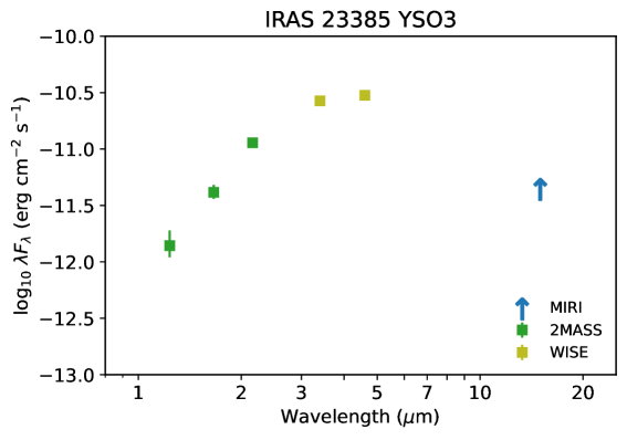
Figure 30: SED of a candidate embedded protostar in the outer Galaxy found by simultaneous MIRI imaging.

C.2 Role of PAH emission affecting ice bands

The MIRI spectra and SEDs may also contain signatures of PAHs. MIRI has the sensitivity to detect these features throughout a cloud. At the position of deeply embedded sources, PAH features were largely undetected with ISO for high-mass protostars (e.g., Gibb et al. 2004) (unless associated with well-known PDRs such as Orion) and with Spitzer for low-mass protostars (Geers et al. 2009). Likely explanations include freeze-out into ices and coagulation to larger PAH systems that do not emit, rather than a lack of UV radiation to excite them. With JWST’s much higher sensitivity, PAH emission may be seen both on and off source, however.

The case of IRAS 23385+6053 provides a particularly illustrative example of how this emission can complicate the analysis of broad ice features in the spectrum. Likely, the PAH emission, which is clearly seen at 11.3 $\mu$m (Beuther et al. 2023), comes from a background cloud and is extincted by ices in the dense envelope surrounding the high-mass protostellar cluster. This makes the 6.2 and 7.7 $\mu$m features hard to detect and they can distort the ice bands. This case serves as a warning for detailed analysis of ice bands in high-mass sources.

Appendix D Mass loss rate determinations and shock model comparison

To obtain more quantitative information on the physical parameters and jet properties, we follow the analysis methods of Caratti o Garatti et al. (2024) for HH 211 in slightly modified form. Rather than using [Fe II] and [S I] line ratios, we take the [Ne II] and [S I] line fluxes to constrain shock characteristics. Figure 31 compares the observed extinction-corrected [Ne II] 12.8 $\mu$m and [S I] 25 $\mu$m fluxes from spectra extracted at the red knot position with the shocks models of Hollenbach & McKee (1989). Assuming that all of the line emission comes from such dissociative shocks, the [Ne II] line constrains the shock velocity to $\sim 40-45$ km s^-1 whereas the [S I] flux suggests the pre-shock total hydrogen density $n_{0}$(H + 2H₂) to be $\sim 10^{5}$ cm^-3 (red lobe). The mass-loss rate indicated by the atomic lines is then

$${\dot{M}}_{\rm atomic}=\mu m_{\rm H}n_{0}\pi r_{j}^{2}v_{\rm tot}$$ (2)

where $\mu$ is the mean atomic weight (1.35), $m_{\rm H}$ is the proton mass, $r_{j}$ is the jet radius, measured to be $\sim$60 au from the jet diameter at the shortest wavelengths where the MIRI angular resolution is the highest and sufficient to resolve the width. The total velocity $v_{\rm tot}$ of $\sim$50 km s^-1 is obtained from the measured jet velocity of $\sim$30 km s^-1 (from ionic lines and from ALMA CO data in the jet), corrected for an inclination of $\sim 50^{o}$ estimated from CO millimeter maps (Yıldız et al. 2015). The inclination could be higher by 10-15^o as estimated from the ALMA continuum disk image, but is unlikely to be lower. This formula gives a typical mass loss rate of ${\dot{M}}_{\rm atomic}=4.5\times 10^{-8}$ M_⊙ yr^-1 for the red lobe.

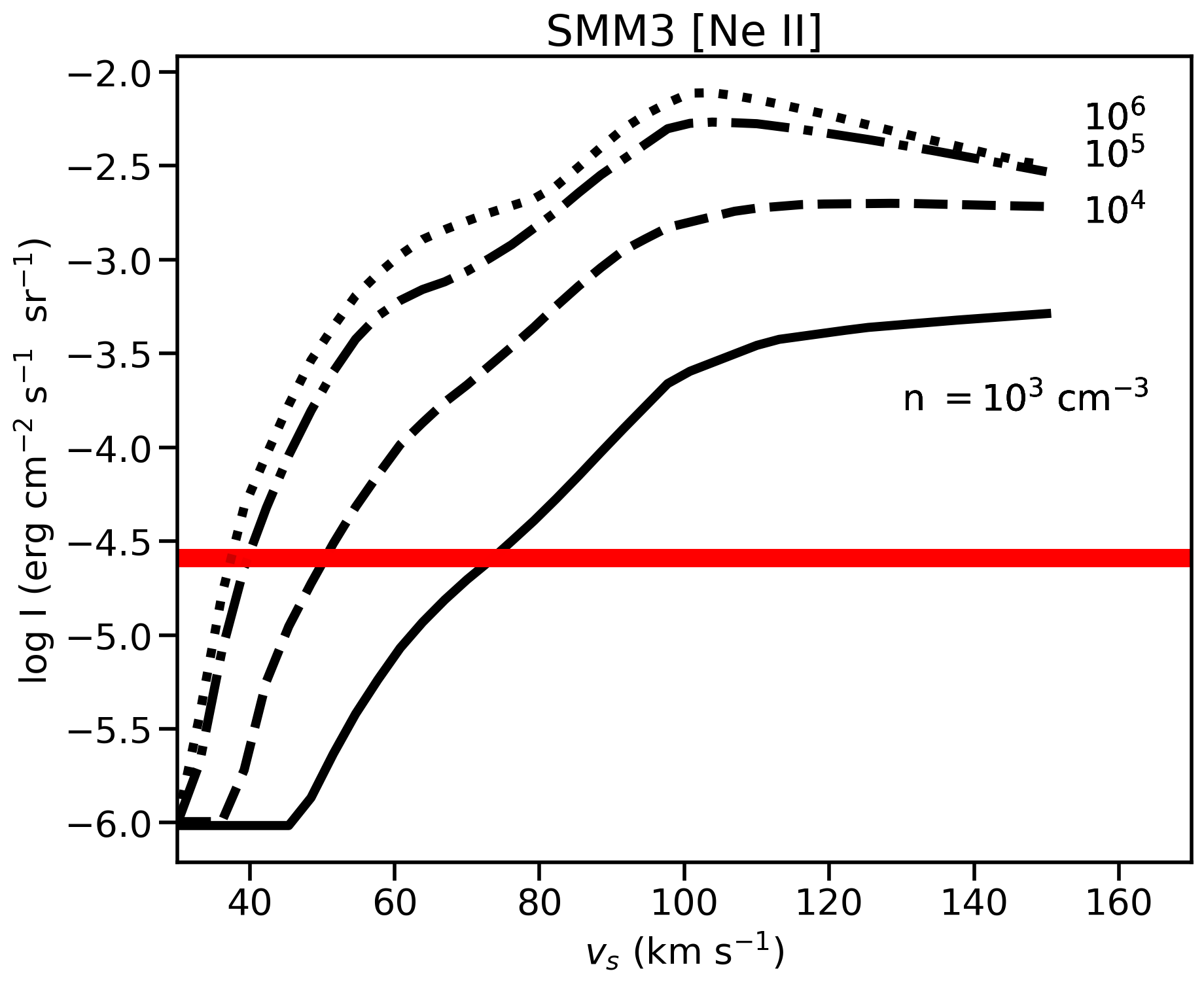
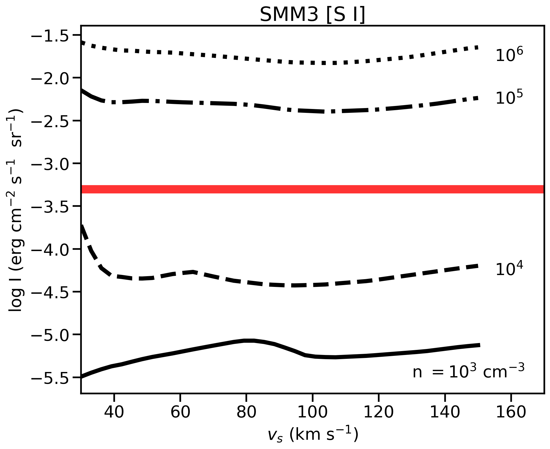
Figure 31: Comparison of the extinction-corrected [Ne II] 12 $\mu$m and [S I] 25 $\mu$m fluxes for SMM3 in the red outflow lobe with shock models of Hollenbach & McKee (1989) as function of shock velocity and pre-shock density. The red horizontal bars indicate the observed values for the red lobe of SMM3.

An alternative route to getting the mass outflow rates is to use the flux of the [O I] 63 $\mu$m line, which is the main coolant of the jet (Hollenbach 1985). Using the measured [O I] 63 $\mu$m flux from Herschel-PACS of $1\times 10^{-2}$ L_⊙ summed over the $\sim$9^′′ spaxels where the line is detected gives a mass loss rate $\dot{M}$ of $\sim(0.6-1)\times 10^{-6}$ M_⊙ yr^-1 (Mottram et al. 2017; Karska et al. 2018), significantly higher than the value inferred above.

Watson et al. (2016) found that the [Fe II] 26 $\mu$m ground state fine structure line can be used as a proxy for [O I] through the following relation:

$${\dot{M}}_{\rm atomic}=1.4\times 10^{-3}L({\rm Fe}\ 26\mu{\rm m})/L_{\odot}.$$ (3)

Using the extinction corrected 26 $\mu$m [Fe II] luminosities of $3.5\times 10^{-6}$ and $7.5\times 10^{-6}$ L_⊙ for the red- and blue-shifted positions where H₂ was extracted gives mass loss rates of ${\dot{M}}_{\rm atomic}=0.5\times 10^{-8}$ and $1.1\times 10^{-8}$ M_⊙ yr^-1, respectively, more in line with those found from [Ne II] + [S I]. However, these values seem low compared with the Spitzer studies by Watson et al. (2016) using this line, also given the significant luminosity of SMM3, but this could be due to the much smaller area over which the [Fe II] line flux is measured compared with Spitzer data. Summing over the entire $\sim 7^{\prime\prime}\times 7^{\prime\prime}$ MRS Channel 4 FOV (comparable to the Spitzer-IRS aperture) gives a extinction-corrected [Fe II] 26 line luminosity of $6.1\times 10^{-5}$ L_⊙, which translates to ${\dot{M}}_{\rm atomic}=8.6\times 10^{-8}$ M_⊙ yr^-1. This value is indeed significantly higher than that derived for a single position, but is still an order of magnitude lower than that derived from [O I]. A similar difference was found for HH 211.

Note that the [O I] determination should be considered as an upper limit for various reasons. The Hollenbach (1985) model assumes a single knot whereas there may be many more in the beam, as is known for the case of SMM3 (Tychoniec et al. 2021) (Le Gouellec et al., in prep.). For the case of SMM3, the [O I] 63 $\mu$m flux is also likely affected by extended emission from the nearby SMM6 source in the large Herschel-PACS aperture; the peak [O I] emission indeed seems somewhat off centered from the SMM3 source position (Karska et al. 2013). Finally, optical depth and foreground absorption of the [O I] 63 $\mu$m line can also affect the estimate. In summary, this example illustrates the uncertainties and pitfalls associated with the different methods and the need to recalibrate some of the relations for the higher spatial resolution data provided by JWST.

Appendix E Which line traces what?

Table 5 summarizes the commonly observed mid-infrared lines in protostellar systems and their proposed origin based on the JWST data.

Table 5: Overview of mid-infrared lines commonly detected in protostellar systems

Species	Transition	$\lambda$	$E_{\rm u}/k$	Typea	Origin
	$u-l$	($\mu$m)	(K)
[Fe II]	a${}^{4}{\rm F}_{9/2}$-a${}^{6}{\rm D}_{9/2}$	5.3402	2694	R	Jet
	a${}^{4}{\rm F}_{7/2}$-a${}^{4}{\rm F}_{9/2}$	17.9232	3496		Jet
	a${}^{4}{\rm F}_{5/2}$-a${}^{4}{\rm F}_{7/2}$	24.5019	4083		Jet
	a${}^{6}{\rm D}_{7/2}$-a${}^{6}{\rm D}_{9/2}$	25.9884	554		Jet, Entrained gas
[Fe I]	${}^{5}{\rm D}_{3}$-${}^{5}{\rm D}_{4}$	24.0423	600	R	Jet
[Ni II]	${}^{2}{\rm D}_{3/2}$-${}^{2}{\rm D}_{5/2}$	6.6360	2168	R	Jet
[Ne II]	${}^{2}{\rm P}_{1/2}$-${}^{2}{\rm P}_{3/2}$	12.8135	1123	V	Jet, Photoionized gas
[Ne III]	${}^{3}{\rm P}_{1}$-${}^{3}{\rm P}_{2}$	15.5551	925	V	Jet, Photoionized gas
[Ar II]	${}^{2}{\rm P}_{1/2}$-${}^{2}{\rm P}_{3/2}$	6.9853	2060	V	Jet, Photoionized gas
[S I]	${}^{3}{\rm P}_{1}$-${}^{3}{\rm P}_{2}$	25.2490	570	SR	Jet, Wind?
H2b	S(1)	17.0348	170	V	Wind, Entrained gas
	S(5)	6.9095	2504	V	Wind, Jet
CO	$v=1-0$ $\geq$P(24)	4.9–5.2	4600–8000	V	Jet, Shockd
H2O	$v_{2}$=1-0 rovib	5.5–7.5	2300–$>$4000	V	Shock, Hot cored
	$v$=0-0 warm	11–18c	2600–$>$8000	V	Shock, Hot cored
	$v$=0-0 cold	20–27c	1100–4000	V	Hot cored
CO2	$v_{2}$=1-0	14.4–15.6	960–1500	V	Hot cored, Outflow
HCN	$v_{2}$=1-0	13.5–14.5	1000–1500	V	Hot cored
C2H2	$v_{5}$=1-0	13.0–14.5	1000–2000	V	Hot cored
OH	$v$=0-0	9–27	10000–40000	V	Shock, UV-irradiated gasd

^a R=Refractory, SR=Semi-Refractory, V=Volatile.
^b Only some example H₂ lines in $v$=0 are listed
^c Lines from warm H₂O also at longer wavelengths
^d Some contribution from young disk possible in Class I sources

Appendix F IRAS 18089 continuum, silicate and H₂O ice subtraction

In order to analyze the 7–9 $\mu$m range for absorption of various ices, first the continuum and silicate features need to be subtracted from the IRAS 18089 spectrum presented in Fig. 21. The method consists of applying the following equation to simultaneously fit both components

$${F=F_{0}{\rm exp}(-\tau_{\rm dust})+F_{\rm cold}}$$ (4)

where $F_{0}$ is assumed to be a blackbody emission with a temperature of 700 K, originating from the warm envelope region. $\tau_{\rm dust}$ is the optical depth from the dust along the line of sight, which is given by $\tau_{\rm dust}=\rho_{\rm dust}\kappa_{\rm dust}$, where $\rho_{\rm dust}$ is the dust column density in cm^-2 g, and $\kappa_{\rm dust}$ is the dust mass absorption coefficient in cm² g^-1. Finally, an additional source of emission coming from a cold envelope at $T=35\leavevmode\nobreak\$K is used to fit (by eye) the spectrum at wavelengths above 20 $\mu$m where cold dust emission starts playing a major role.

The dust properties used in this paper follow previous studies by Sargent et al. (2009); Boogert et al. (2008); McClure et al. (2023) and Rocha et al. (2024). They consist of adopting olivine (MgFeSiO₄) and pyroxene (Mg_0.7Fe_0.3SiO₃) stoichiometries as representative of the dust. The optical constants of these materials were taken from Dorschner et al. (1995). In addition, a grain-shape correction was performed by adopting a distribution of hollow spheres (DHS Min et al. 2005), and a size distribution ranging from $a_{\rm min}=0.1$ $\mu$m to $a_{\rm max}=1.0$ $\mu$m. The calculations of the dust opacities with those properties are executed with the OpTool software (Dominik et al. 2021).

Figure 32 (top) shows the continuum and silicate absorption profiles for IRAS 18089. The contributions of the two silicate (pyroxene + olivine) bands at 9.7 and 18 $\mu$m are seen. The 9.7 $\mu$m absorption is slightly overestimated in the model to account for the excess between 8 and 9 $\mu$m. Part of this missing absorption at 9–10 $\mu$m may be due to some superposed silicate emission from an inner warm envelope or disk. Since our primary interest is in the 7–9 $\mu$m range, the precise details do not matter. The 18 $\mu$m band matches well the observations but the long wavelength wing is overpredicted by the model. This is compensated by the cold blackbody emission above 20 $\mu$m.

Once the continuum and silicate are estimated, the spectrum is converted to an optical depth scale using the equation $\tau=-$ln($F_{\rm obs}/F_{\rm cont}$), where $F_{\rm obs}$ is the observed flux and $F_{\rm cont}$ is the continuum flux which in this approach, which includes the silicate absorption profile. The result is presented in Figure 32 (bottom).

Based on this continuum model with the silicate features, we obtain $\tau_{9.7}$ = 9.2. Assuming an extinction law similar to dense star-forming regions in Perseus ($A_{V}=28.6\times\tau_{9.7}$ Boogert et al. 2013), the derived visual extinction is $A_{V}\sim$263 mag (see Appendix G for more details). While such a huge extinction correction would be required for any emission features arising from the inner region (see van Gelder et al. 2024a, for a detailed discussion), this is not the case for absorption bands from the ices/dust. For example, independent analyses of $L-$band spectra from protostars in the Serpens molecular cloud were performed by Pontoppidan et al. (2004) with extinction correction and Perotti et al. (2020) without correction. Both methods result in equivalent optical depths after continuum removal.

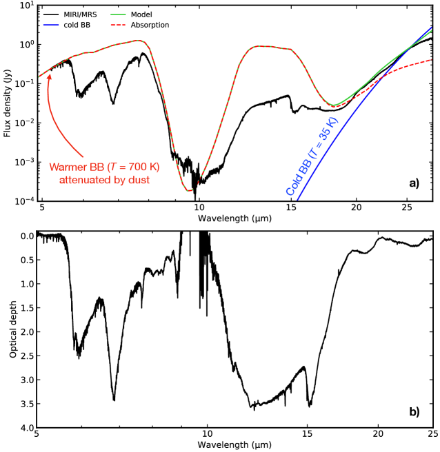
Figure 32: IRAS 18089 spectrum before and after global continuum and silicate subtraction. Panel a (top) shows the simplified model for IRAS 18089 given by a warm (red line) and cold (blue line) blackbody emission. Panel b (bottom) displays the optical depth scale of IRAS 18089 with both continuum and silicate subtracted.

The next step is to fit and remove the H₂O ice features. In the MIRI range, H₂O ice has two prominent and broad features, the bending mode around 6 and the libration mode at 12 $\mu$m. Similarly to the dust properties, the analysis of the H₂O ice features has been performed using a distribution of grain-shape corrected spectra adopting the DHS approach and different temperatures to account for the temperature gradient of the source. The result is presented in Figure 33. The fit using particles ranging from 0.1 to 1.0 $\mu$m in size is indicated by the grey line. Despite the good fit to the short wavelength range of the 12 $\mu$m band, it leaves a strong absorption excess unexplained at longer wavelengths. For this reason, we considered an additional size distribution of larger grains, ranging from 1.0 to 2.0 $\mu$m. In particular, we assumed that the hot ice (160 K) component is dominated by smaller grains, whereas the cold ice (15 K) is represented by larger grains. In this combined case, the fit is equally good at short wavelengths and reduces the excess at longer wavelengths.

The fit to the various ice features in the 7–9 $\mu$m range is presented in Figure 22. The fit to the 6.85 $\mu$m feature, consisting of both NH${}_{4}^{+}$ and CH₃OH ice, is contained in Figure 35. Following Slavicinska et al. (2025b), ammonium hydrosulfide salt NH₄SH provides the best fit to the feature; the adopted band strength is 3.6$\times$ 10^-17 cm molecule^-1. This allows us to quantify the N-budget in ices. In this calculation, the overall N abundance is assumed to be $6.3\times 10^{-5}$ (Przybilla et al. 2008) and the total hydrogen column along the line of sight $N_{\rm H}=3.6\times 10^{23}$ cm^-2 based on the above extinction $A_{V}$=263 mag and $N_{\rm H}/A_{V}=1.37\times 10^{21}$ cm^-2 mag^-1 (Evans et al. 2009).

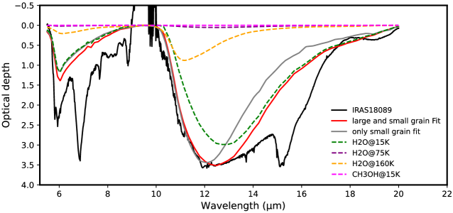
Figure 33: Simplified H₂O ice model for IRAS 18089, after subtraction of the global continuum and silicate band. The small-grain only fit is indicated by the grey line, and the combined (large and small) grain population is shown by the red line. The dashed lines show the H₂O ice components for the combined population model.

Table 6 summarizes the column densities of the molecules used to produce the fit in Figure 22 and 35. The column density used to fit the newly detected 8.38 $\mu$m feature will be presented in a future paper dedicated to the analysis of this band (Rocha et al., in prep.).

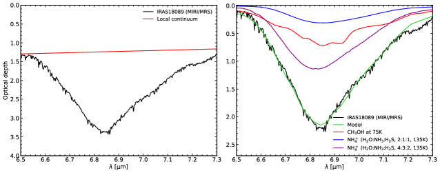
Figure 35: 6.85 $\mu$m feature towards IRAS18089. The left panel shows the local continuum subtraction and the right panel displays the best fit and the individual NH${}_{4}^{+}$ components and warm CH₃OH ice.

Table 6: Ice column densities corresponding to the best fit of the IRAS 18089 spectrum

Species	Name	$N$
		($10^{17}$ cm-2)
H2O	water	282.3$\pm$70.5
CH4	methane	5.3$\pm$1.3
SO2	sulfur dioxide	0.3$\pm$0.1
OCN-	cyanate ion	5.3$\pm$1.5
NH${}_{4}^{+}$	ammonium ion	33.0$\pm$4.0
HCOO-	formate ion	1.1$\pm$0.3
H2CO	formaldehyde	28.2$\pm$7.1
CH3OH	methanol	50.4$\pm$12.7
HCOOH	formic acid	2.9$\pm$0.7
CH3CHO	acetaldehyde	1.9$\pm$0.5
CH3CH2OH	ethanol	4.2$\pm$1.1
CH3OCHO	methyl formate	0.9$\pm$0.2
CH3COOH	acetic acid	$<$2
CH3OCH3	dimethyl ether	2.8$\pm$0.7
CH3COCH3	acetone	0.7$\pm$0.2

Appendix G Extinction determinations

Most lines and diagnostics require a correction for extinction, which is substantial for these deeply embedded sources. As discussed in detail by van Gelder et al. (2024b, a) the correction consists of two parts: (i) an absolute extinction ($\tau_{\rm dust}$) based on an extinction law; and (ii) differential extinction caused by various ice absorption bands and silicates ($\tau_{\rm ice,silicates}$) at specific wavelengths.

Several formulations of the extinction law exist in the literature (e.g., Weingartner & Draine 2001; Gordon et al. 2023); they are usually optimized for diffuse cloud dust from UV to infrared and include already some form of silicate absorption. The JOYS+ papers to date use either the McClure (2009) law or the Pontoppidan et al. (2024a) law (KP5), which have been developed for the mid-infrared extinction due to dust in dense clouds. The KP5 relation contains also some generic ice features as well as a deeper silicate absorption than the McClure (2009) law.

In the JOYS+ papers, the local ice extinction is usually estimated from the observed spectrum itself and can be substantial: for example, the gaseous CO₂ $P-$branch lines can be fully extincted by the CO₂ ice band, but this does not hold for the $R-$branch lines (Francis et al. 2024). This example also illustrates that the appropriate extinction to use depends on the origin of the emission: for example, hot core emission from molecules such as CO₂ and H I recombination lines originating close to the protostellar embryo experience more extinction than lines coming from an outflow cavity.

One way to determine the absolute extinction in units of $A_{K}$ or $A_{V}$ is to use one of the above global extinction laws, following the procedure as described in, for example, Appendix C of van Gelder et al. (2024b). There are at least three other methods that can and have been adopted. The first method is to measure just the optical depth of the silicate feature at 9.7 $\mu$m, $\tau_{\rm 9.7}$, which represents the total extinction along the line of sight to the dust sublimation radius, very close to the protostellar embryo. Its relation with $A_{K}$ has been well calibrated by comparing $\tau_{\rm 9.7}$ from Spitzer spectra against extinction measurements of reddened background stars behind dense clouds. Boogert et al. (2013) (their equations (4) and (5)) find that the relation changes between diffuse cloud ($A_{V}\lesssim 10$ mag) and dense cloud dust in the Lupus star-forming region. These relations have more recently been confirmed for other clouds by Madden et al. (2022). Assuming $A_{V}/A_{K}$=7.7 as appropriate for $R_{V}=5.5$ (Cardelli et al. 1989), the Boogert et al. (2013) diffuse cloud relation leads to $A_{V}=18.5\times\tau_{\rm 9.7}$. For dense cloud dust, it becomes $A_{V}=28.6\times\tau_{\rm 9.7}$. The latter relation is appropriate for deeply embedded low-mass Class 0 and high-mass sources, and has indeed been used for IRAS 18089 in Appendix F. Class I sources have lower extinctions but generally still well above 10 mag. However, use of the dense cloud relation has been found to lead to unreasonably high accretion rates, hence the diffuse cloud relation has been adopted for Class I sources in § 4.2.

A second, related method is to use the observed relations of ice optical depths with $A_{V}$ (Whittet et al. 2001; Boogert et al. 2015). The best-known relation is that of the 3 $\mu$m water ice feature, $\tau_{3.0}$, versus $A_{K}$ calibrated by Boogert et al. (2013); Madden et al. (2022) for dense clouds. Since the 3 $\mu$m ice band is often saturated in the most deeply embedded JOYS+ sources, an alternative is to use the 15 $\mu$m CO₂ ice band $\tau_{15}$ (Bergin et al. 2005; Whittet et al. 2009) which can now be readily observed with JWST. Further calibration of the $\tau_{15}$ versus $A_{K}$ relation for dense clouds is warranted.

A third measure of the extinction can be obtained from the excitation of H₂: rotational diagrams using lines in the MIRI wavelength range show that the S(3) line flux at 9.66 $\mu$m clearly falls below that of the neighboring H₂ lines due to enhanced silicate extinction, as has also been found in ISO and Spitzer data. Various papers show how both the extinction and the H₂ ortho-to-para ratio can be fitted simultaneously to H₂ rotation diagrams to obtain a value of $A_{V}$ (e.g., Neufeld et al. 2006; Giannini et al. 2011; Francis et al. 2025; Okoda et al. 2025). This extinction value should be appropriate for any emission lines originating from the outflow and its cavity. If NIRSpec data are available, one can add higher excitation H₂ lines at shorter wavelengths to this analysis.

A more effective way to use NIRSpec data may, however, be to obtain an extinction estimate from atomic or molecular lines lines that originate from the same upper level; the MIRI range does not contain such line pairs. The intrinsic ratio of these line pairs depends only on their Einstein $A$ values and frequencies, so the difference between observed and theoretical flux ratios directly gives the local reddening at the corresponding wavelengths. For H₂, the 1–0 S(1) line at 2.12 $\mu$m and 1–0 O(5) line at 3.23 $\mu$m are a well-known line pair that can be used for this purpose: entire outflow extinction maps can even be obtained using narrow-band filters containing these lines with NIRCam (Ray et al. 2023; Caratti o Garatti et al. 2024). Similarly [Fe II], H I or other atomic lines originating from the same upper level in the 0.4–2 $\mu$m range can be useful extinction tracers in regions that are not too extincted (e.g., Giannini et al. 2015). Note that for JOYS+ sources, high spectral resolution NIRSpec data are limited to $>$3 $\mu$m. Assani et al. (2025) have recently introduced a procedure for comparing extinction estimates from [Fe II] NIRSpec and MIRI data that warrants further exploration.

As noted in Appendix F, no extinction correction is applied to absorption features of ices or silicates since they directly measure the column along the line of sight. Molecular absorption lines originating in hot core gas lying interior to the outer icy envelope would require an extinction correction, but in practice only the differential correction due to ices (e.g., the CO₂ gas + ice case) has been applied in the JOYS papers (e.g., van Gelder et al. 2024a). Also, a covering fraction of unity by the absorbing material is assumed (see also § 3.5). Since the main interest is in relative column density ratios, rather than absolute ones, this should not change significantly any conclusions unless the lines are heavily saturated.

In this paper all of these methods to determine extinction have been used, often to be consistent with earlier JOYS papers. A systematic comparison between them is left for a future paper. It should be noted that differences in absolute values of, most notably, accretion rates can be substantial depending on the adopted method.