rd2d: Causal Inference in Boundary Discontinuity Designs

Abstract

Boundary discontinuity designs—also known as Multi-Score Regression Discontinuity (RD) designs, with Geographic RD designs as a prominent example—are often used in empirical research to learn about causal treatment effects along a continuous assignment boundary defined by a bivariate score. This article introduces the R package rd2d, which implements and extends the methodological results developed in Cattaneo et al. (2025) for boundary discontinuity designs. The package employs local polynomial estimation and inference using either the bivariate score or a univariate distance-to-boundary metric. It features novel data-driven bandwidth selection procedures, and offers both pointwise and uniform estimation and inference along the assignment boundary. The numerical performance of the package is demonstrated through a simulation study.

Keywords: treatment effects, regression discontinuity designs, nonparametric regression.

1 Introduction

Regression Discontinuity (RD) designs are commonly used for treatment effect estimation and causal inference in quantitative sciences (see Cattaneo and Titiunik, 2022, and references therein). In their canonical form, each unit $i\in\{1,2,\cdots,n\}$ is assigned to control ($T_{i}=0$) or treatment ($T_{i}=1$) according to the discontinuous rule $T_{i}=\mathds{1}(X_{i}\geq c)$, where $X_{i}$ denotes a scalar score variable, $c$ denotes a scalar cutoff, and $\mathds{1}(\cdot)$ is the indicator function. The key idea underlying all RD designs is that units with a score near the cutoff determining treatment assignment are comparable in terms of all pretreatment observables and unobservable characteristics, the only difference being that some units are assigned to control ($X_{i}<c$) while other are assigned to treatment ($X_{i}\geq c$). Therefore, in the absence of score manipulation, units having a score near (but on different sides of) the cutoff can be used as counterfactual of each other to learn about causal treatment effects.

Boundary discontinuity designs generalize the canonical RD design to allow for a multi-dimensional score variable (Papay et al., 2011; Reardon and Robinson, 2012; Keele and Titiunik, 2015). The most common case is a bivariate score $\mathbf{X}_{i}=(X_{1i},X_{2i})^{\top}$ with an assignment boundary curve $\mathcal{B}$ on its support. For example, Londoño-Vélez et al. (2020) study the effect of a Colombian social program where $X_{1i}$ is a poverty index and $X_{2i}$ is an exam grade, for each student $i$, and where eligibility for receiving the treatment required either a minimum poverty index ($X_{1i}\geq c_{1}$) or a minimum exam grade ($X_{2i}\geq c_{2}$). Therefore, in their application, the boundary determining treatment is $\mathcal{B}=\{(X_{1i},X_{2i}):\{X_{1i}\geq c_{1}\text{ and }X_{2i}=c_{2}\}\cup\{X_{1i}=c_{1}\text{ and }X_{2i}\geq c_{2}\}\}$. This type of bivariate RD designs, where each score component has its own cutoff, is illustrated in Figure 1(a). Another prototypical class of boundary discontinuity designs are the Geographic RD designs: for instance, Keele and Titiunik (2015) study the effect of political advertisements on voter turnout during a presidential campaign by leveraging sharp discontinuities in exposure to presidential ads induced across geographic media market boundaries. Figure 1(b) illustrates a generic example of a Geographic RD design employing the boundary separating two US states. Jardim et al. (2024) gives another recent empirical application of a boundary discontinuity design in the context of labor markets, and provides further references. See Cattaneo et al. (2020, 2024) for a two-part practical introductory monograph.

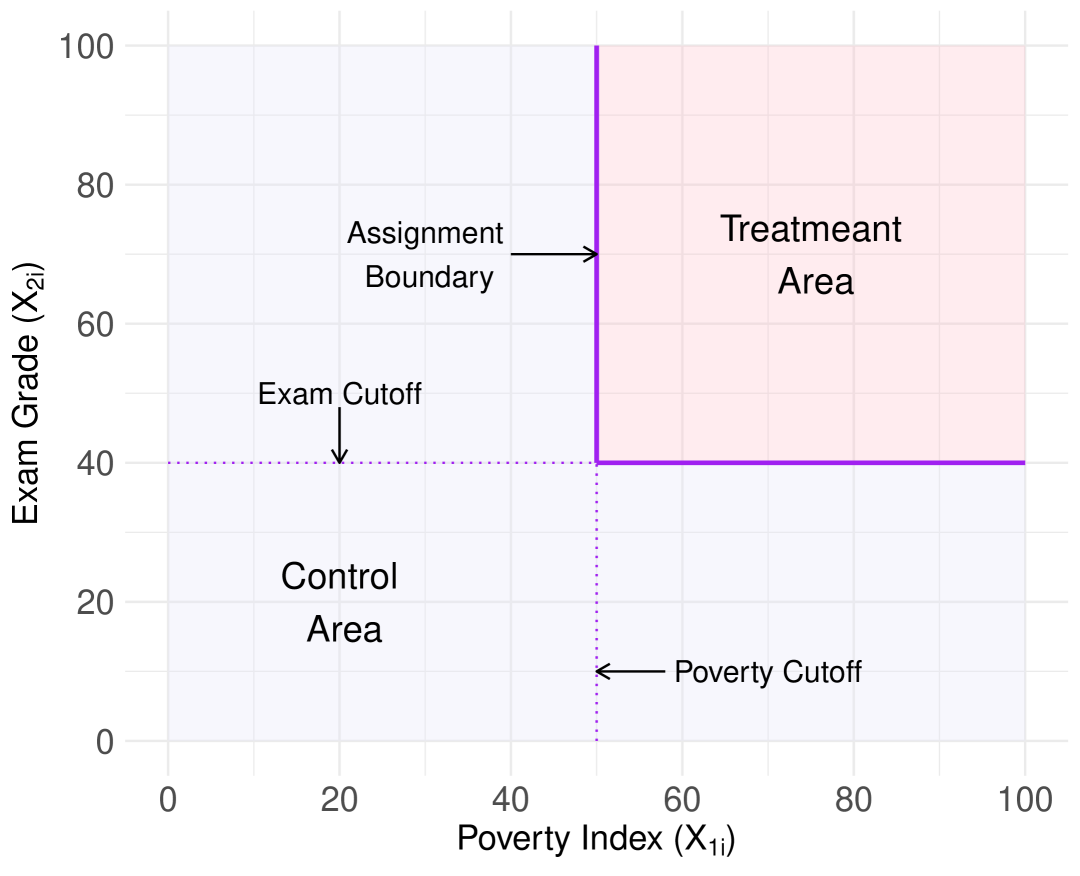
(a) Two-Score RD Design.

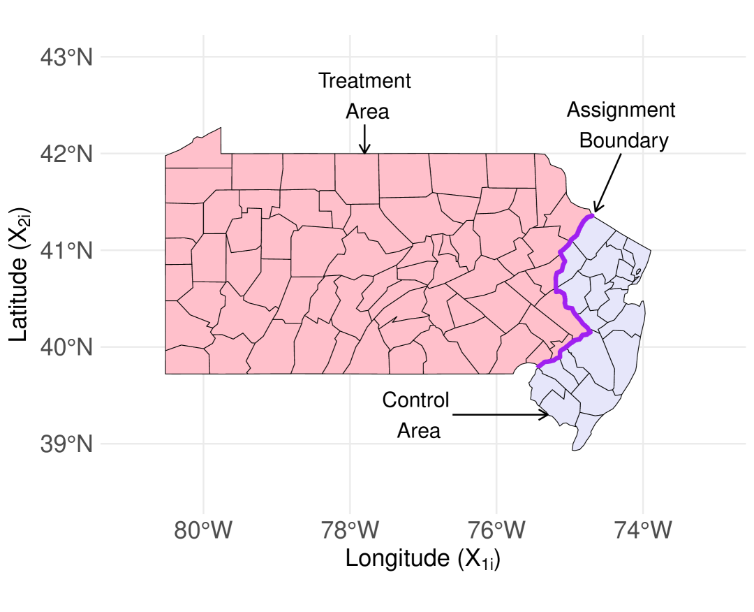
(b) Geographic RD Design.

Figure 1: Two Examples of Boundary Discontinuity Designs

While classical RD designs based on a scalar score are well-understood in the literature, boundary discontinuity designs are surprisingly less studied. Methodological developments have lagged empirical practice for a while, leading to different approaches in practice, but without a foundational understanding of their relative merits. Cattaneo et al. (2025) address this gap in the literature by studying the properties of two leading approaches often used in empirical research leveraging boundary discontinuity designs:

• the location-based approach employs bivariate local polynomial regression analysis based on the bivariate location score relative to each point on the boundary $\mathcal{B}$; and

• the distance-based approach employs univariate local polynomial regression analysis based on a scalar score constructed as distance to each point on the boundary $\mathcal{B}$.

Cattaneo et al. (2025) study the two methodologies, and establish novel identification, estimation and inference results, both pointwise for each point on $\mathcal{B}$ and uniformly over $\mathcal{B}$. Importantly, they demonstrate that the distance-based approach can exhibit a large bias near kinks or other irregularities in the assignment boundary $\mathcal{B}$, while the location-based approach remains valid even in those cases. Based on their findings, it is recommended to employ the bivariate location-based approach whenever possible, but their results provide foundational theoretical guidance for both empirical approaches.

This article introduces the R software package rd2d, which expands and implements the methodological results in Cattaneo et al. (2025), thereby offering data-driven general-purpose methods for the analysis and interpretation of boundary discontinuity designs. The package includes the following four functions.

• rd2d(). This function implements location-based local polynomial regression analysis for estimation and inference of causal treatment effects in boundary discontinuity designs. For the $n$ units of analysis, the function takes as inputs their outcomes $\mathbf{Y}=(Y_{i}:i=1,\cdots,n)^{\top}$, their bivariate location scores $\mathbf{X}=[\mathbf{X}_{i}=(X_{1i},X_{2i})^{\top}:i=1,\cdots,n]^{\top}$, their treatment assignment indicators $\mathbf{T}=(T_{i}:i=1,\cdots,n)^{\top}$, and a collection of cutoffs $\mathbf{b}=[\mathbf{b}_{j}=(b_{1j},b_{2j})^{\top}:j=1,\cdots,J]^{\top}$ on the boundary $\mathcal{B}$ determining treatment assignment. The function then implements estimation and (robust bias-corrected) inference via bivariate local polynomial regression, both pointwise and uniformly over the cutoffs $\mathbf{b}_{j}\in\mathcal{B}$. As it is customary in nonparametric regression settings, the function requires specifying a bandwidth (localization) parameter: if not provided by the user, it is selected via the companion function rdbw2d() for data-driven bandwidth selection.

• rdbw2d(). This function employs mean square error (MSE) approximations to implement (approximate) MSE-optimal bandwidth selection for treatment effect estimation and inference in boundary discontinuity designs. It provides second-generation direct plug-in (DPI) rules (Härdle et al., 2004; Wand and Jones, 1994), incorporating several regularization schemes.

• rd2d.dist(). This function implements distance-based local polynomial regression analysis for estimation and inference of causal treatment effects in boundary discontinuity designs. For the $n$ units of analysis, the function takes as inputs their outcomes $\mathbf{Y}=(Y_{i}:i=1,\cdots,n)^{\top}$, their scalar distance scores $\mathbf{D}=[[D_{i}(\mathbf{b}_{j}):j=1,\cdots,J]^{\top}:i=1,\cdots,n]^{\top}$, and a collection of cutoffs $\mathbf{b}=[\mathbf{b}_{j}=(b_{1j},b_{2j})^{\top}:j=1,\cdots,J]^{\top}$ on the boundary $\mathcal{B}$. That is, $T_{i}(\mathbf{b}_{j})=\mathds{1}(D_{i}(\mathbf{b}_{j})\geq 0)$ denotes the treatment assignment for unit $i$ relative to cutoff $\mathbf{b}_{j}\in\mathcal{B}$. This function also implements estimation and (robust bias-corrected) inference via univariate local polynomial regression, both pointwise and uniformly over the cutoffs $\mathbf{b}_{j}\in\mathcal{B}$. If the bandwidth (localization) parameter is not provided by the user, then it is chosen via the companion function rdbw2d.dist() for data-driven bandwidth selection.

• rdbw2d.dist(). This function implements rule-of-thumb (ROT) bandwidth selection rules, depending on the specific assumptions on $\mathcal{B}$ imposed. More precisely, depending on whether the assignment boundary $\mathcal{B}$ is assumed to be smooth or not, different ROT bandwidth selectors are implemented as supported by the underlying theoretical results in Cattaneo et al. (2025). Unfortunately, when $\mathcal{B}$ exhibits kinks or other irregularities, it is difficult to develop MSE-optimal bandwidth selection, in which case the function reverts back to a simple ROT implementation based on a rate-optimality criteria.

The methods print() and summary() are supported for objects returned by rd2d(), rdbw2d(), rd2d.dist(), and rdbw2d.dist(). We also demonstrate how to use the outputs to generate useful plots for empirical work, depicting treatment effect estimation, confidence intervals, and confidence bands, along the treatment assignment boundary $\mathcal{B}$.

In addition, the four functions in the package rd2d offer several practically relevant features, including (i) heteroskedasticity-robust and cluster-robust variance estimation, (ii) explicit regularization for the presence of mass points in the bivariate location score $\mathbf{X}_{i}$ or the univariate distance score $D_{i}(\mathbf{b}_{j})$, and (iii) explicit regularization accounting for specific extreme shape features of the underlying unknown conditional expectation functions for bandwidth selection. In the case of rd2d(), the bivariate location-based approach, the data-driven point estimator is approximately MSE-optimal, while in the case of rd2d.dist(), the univariate distance-based approach, the rate-optimality of the data-driven point estimator depends on the underlying geometry of the assignment boundary $\mathcal{B}$. Putting aside the induced bias by the possibly non-smooth $\mathcal{B}$, both functions offer pointwise (for each $\mathbf{b}_{j}\in\mathcal{B}$) and uniform (over $\mathcal{B}$) robust bias-corrected inference (Calonico et al., 2018, 2022).

The main contribution of this article is to introduce and discuss the first general-purpose software implementation of (MSE-optimal) treatment effect estimation and (pointwise and uniform) uncertainty quantification methods for boundary discontinuity designs, given by the R package rd2d. To this end, the article develops second-generating DPI rules for bandwidth selection, along with principled regularization schemes for specific empirically relevant settings (e.g., mass points in $\mathbf{X}_{i}$) and practically relevant variance estimators (e.g., cluster-robust).

The rest of the paper proceeds as follows. Section 2 reviews the main methodological contributions in Cattaneo et al. (2025), and presents additional results related to bandwidth selection and regularized implementation. Section 3 demonstrates the performance of the R package rd2d using a simulation study with a data generated process calibrated using the data in Londoño-Vélez et al. (2020). Section 4 concludes. Replication codes, background references, and other information related the software package rd2d can be found at: https://rdpackages.github.io/rd2d/.

2 Methods and Implementation

We employ standard potential outcomes notation. Suppose that $(Y_{i}(0),Y_{i}(1),\mathbf{X}_{i}^{\top})^{\top}$, $i=1,2,\dots,n$, is a random sample, where $Y_{i}(0)$ and $Y_{i}(1)$ denote the scalar potential outcomes for unit $i$ under control and treatment assignment, respectively. Units are assigned to control group or treatment group according to their bivariate location score $\mathbf{X}_{i}=(X_{1i},X_{2i})^{\top}$ relative to a known one-dimensional boundary $\mathcal{B}$ splitting the support of $\mathbf{X}_{i}$ in two disjoint regions: $\mathcal{A}_{0}$ denotes the control region, and $\mathcal{A}_{1}$ denotes the treatment region. Thus, $\mathcal{B}=\mathtt{bd}(\mathcal{A}_{0})\cap\mathtt{bd}(\mathcal{A}_{1})$, where $\mathtt{bd}(\mathcal{A}_{t})$ denotes the boundary of the set $\mathcal{A}_{t}$. The observed response variable is $Y_{i}=(1-T_{i})\cdot Y_{i}(0)+T_{i}\cdot Y_{i}(1)$, where $T_{i}=\mathds{1}(\mathbf{X}_{i}\in\mathcal{A}_{1})$. Without loss of generality, we assume that the boundary belongs to the treatment group, that is, $\mathtt{bd}(\mathcal{A}_{1})\subset\mathcal{A}_{1}$ and $\mathcal{B}\cap\mathcal{A}_{0}=\emptyset$. Figure 1 gives two graphical examples.

The causal parameter of interest is the average treatment effect curve along the boundary:

$$\tau(\mathbf{x})=\mathbb{E}[Y_{i}(1)-Y_{i}(0)|\mathbf{X}_{i}=\mathbf{x}],\qquad\mathbf{x}\in\mathcal{B}.$$

Identification follows directly by the usual continuity assumptions invoked in canonical RD designs (Hahn et al., 2001):

$$\tau(\mathbf{x})=\lim_{\mathbf{u}\to\mathbf{x},\mathbf{u}\in\mathcal{A}_{1}}\mu_{1}(\mathbf{u})-\lim_{\mathbf{u}\to\mathbf{x},\mathbf{u}\in\mathcal{A}_{0}}\mu_{0}(\mathbf{u}),\qquad\mathbf{x}\in\mathcal{B},$$

where $\mu_{t}(\mathbf{x})=\mathbb{E}[Y_{i}(t)|\mathbf{X}_{i}=\mathbf{x}]=\mathbb{E}[Y_{i}|\mathbf{X}_{i}=\mathbf{x},T_{i}=t]$, $t\in\{0,1\}$, are assumed to be smooth functions. See Papay et al. (2011), Reardon and Robinson (2012), Keele and Titiunik (2015), and references therein.

For implementation, the continuous assignment boundary $\mathcal{B}$ is first discretized into $J$ cutoff points $\mathbf{b}=(\mathbf{b}_{1},\cdots,\mathbf{b}_{J})^{\top}$ with $\mathbf{b}_{j}\in\mathcal{B}$ for all $j=1,\dots,J$. Then, the empirical analysis is conducted pointwise for each cutoff or uniformly over all cutoffs, employing either the bivariate location score $\mathbf{X}_{i}$ directly, or an induced univariate distance to each cutoff point. See Cattaneo et al. (2024, Section 5) for an introductory discussion.

Following the methodological recommendations in Cattaneo et al. (2025), most of the discussion focuses on location-based methods via bivariate local polynomial regression based on the data $(Y_{i},\mathbf{X}_{i}^{\top})^{\top}$, $i=1,\cdots,n$, which are implemented in the functions rd2d() and rdbw2d(). However, given their predominance in empirical work, Section 2.2 also discusses distance-based methods via univariate local polynomial regression, which require a user-chosen scalar distance score to each cutoff point on the assignment boundary, and are implemented in the functions rd2d.dist() and rdbw2d.dist(). We omit assumptions and other technical details in the remaining of the paper, which can be found in the references given.

2.1 Location-Based Methods

The location-based treatment effect curve estimator of $\tau(\mathbf{x})$ is

$$\widehat{\tau}(\mathbf{x})=\mathbf{e}_{1}^{\top}\widehat{\boldsymbol{\beta}}_{1}(\mathbf{x})-\mathbf{e}_{1}^{\top}\widehat{\boldsymbol{\beta}}_{0}(\mathbf{x}),\qquad\mathbf{x}\in\mathcal{B},$$

where, for $t\in\{0,1\}$,

$$\widehat{\boldsymbol{\beta}}_{t}(\mathbf{x})=\operatorname*{arg\,min}_{\boldsymbol{\beta}\in\mathbb{R}^{\mathfrak{p}_{p}+1}}\sum_{i=1}^{n}\big{(}Y_{i}-\mathbf{R}_{p}(\mathbf{X}_{i}-\mathbf{x})^{\top}\boldsymbol{\beta}\big{)}^{2}K_{h}(\mathbf{X}_{i}-\mathbf{x})\mathds{1}(\mathbf{X}_{i}\in\mathcal{A}_{t}),$$

with $\mathfrak{p}_{p}=(2+p)(1+p)/2-1$, $\mathbf{R}_{p}(\mathbf{u})=(1,u_{1},u_{2},u_{1}^{2},u_{2}^{2},u_{1}u_{2},\cdots,u_{1}^{p},u_{2}^{p})^{\top}$ denotes the $p$th order polynomial expansion of the bivariate vector $\mathbf{u}=(u_{1},u_{2})^{\top}$, $K_{h}(\mathbf{u})=K(u_{1}/h,u_{2}/h)/h^{2}$ for a bivariate kernel function $K(\cdot)$, and a bandwidth parameter $h$.

In practice, it is often important to first standardize each dimension of the bivariate location score $\mathbf{X}_{i}=(X_{1i},X_{2i})^{\top}$, and in some applications it may also be useful to allow for different bandwidths for control and treatment groups. Thus, the function rd2d() allows for four different bandwidths: $h_{01}$ is used for $X_{1i}$ and control units, $h_{02}$ is used for $X_{2i}$ and control units, $h_{11}$ is used for $X_{1i}$ and treatment units, and $h_{02}$ is used for $X_{2i}$ and treatment units. The data-driven bandwidth selection function rdbw2d() also allows for both standardization of each dimension of $\mathbf{X}_{i}$ (via the option stdvar=TRUE) and different bandwidth selection for control and treatment regions (via the options bwselect="msetwo" or bwselect="imsetwo"). Thus, the function rdbw2d() can report up to four distinct estimated bandwidths: $(\widehat{h}_{01},\widehat{h}_{02},\widehat{h}_{11},\widehat{h}_{11})$ corresponding to $(h_{01},h_{02},h_{11},h_{11})$. The discussion in this article focuses on a single common bandwidth $h$ for simplicity, but we explain how different MSE-optimal bandwidth are estimated as appropriate. In addition, while the notation does not explicitly reflect clustering, which is a common feature in geographic and other multidimensional RD designs, the package rd2d allows for cluster-robust inference as explained below.

2.1.1 Point Estimation, MSE Expansions, and Bandwidth Choices

Under minimal regularity conditions, the bivariate location-based treatment effect estimator $\widehat{\tau}(\mathbf{x})$ is pointwise and uniform consistent for the treatment effect curve $\tau(\mathbf{x})$ along the assignment boundary: $\widehat{\tau}(\mathbf{x})\to_{\mathbb{P}}\tau(\mathbf{x})$ for each $\mathbf{x}\in\mathcal{B}$, and $\sup_{\mathbf{x}\in\mathcal{B}}|\widehat{\tau}(\mathbf{x})-\tau(\mathbf{x})|\to_{\mathbb{P}}0$, where $\to_{\mathbb{P}}$ denotes convergence in probability as $h\to 0$ and $nh^{2}\to\infty$. Furthermore, under similar regularity conditions, precise (conditional) MSE expansions can be established along $\mathcal{B}$, which can then be used for principled bandwidth selection.

The pointwise (conditional) MSE expansion is

$$\mathbb{E}[(\widehat{\tau}(\mathbf{x})-\tau(\mathbf{x}))^{2}|\mathbf{X}]\approx_{\mathbb{P}}\frac{1}{nh^{2}}V_{\mathbf{x}}+h^{2(p+1)}B_{\mathbf{x}}^{2},$$

where $V_{\mathbf{x}}=V_{1,\mathbf{x}}+V_{0,\mathbf{x}}$ and $B_{\mathbf{x}}=B_{1,\mathbf{x}}-B_{0,\mathbf{x}}$ denote the fixed-$n$ conditional variance and the leading conditional bias of the treatment effect estimator, respectively, and $\approx_{\mathbb{P}}$ denotes equality in probability up to vanishing higher-order terms. More precisely, using standard multi-index notation and least squares algebra, the fixed-$n$ conditional variance and leading conditional bias for each group $t\in\{0,1\}$ are

$$V_{t,\mathbf{x}}=\mathbf{e}_{1}^{\top}\widehat{\boldsymbol{\Gamma}}_{t,\mathbf{x}}^{-1}\boldsymbol{\Sigma}_{t,\mathbf{x},\mathbf{x}}\widehat{\boldsymbol{\Gamma}}_{t,\mathbf{x}}^{-1}\mathbf{e}_{1}\qquad\text{and}\qquad B_{t,\mathbf{x}}=\sum_{|\mathbf{k}|=p+1}\frac{\mu_{t}^{(\mathbf{k})}(\mathbf{x})}{\mathbf{k}!}\mathbf{e}_{1}^{\top}\widehat{\boldsymbol{\Gamma}}_{t,\mathbf{x}}^{-1}\widehat{\boldsymbol{\vartheta}}_{t,\mathbf{x}}(\mathbf{k}),$$

respectively, where

$$\widehat{\boldsymbol{\Gamma}}_{t,\mathbf{x}} =\frac{1}{n}\sum_{i=1}^{n}\mathbf{r}_{p}\big{(}\frac{\mathbf{X}_{i}-\mathbf{x}}{h}\big{)}\mathbf{r}_{p}\big{(}\frac{\mathbf{X}_{i}-\mathbf{x}}{h}\big{)}^{\top}K_{h}(\mathbf{X}_{i}-\mathbf{x})\mathds{1}(\mathbf{X}_{i}\in\mathcal{A}_{t}),$$

$$\boldsymbol{\Sigma}_{t,\mathbf{x},\mathbf{x}} =\frac{h^{2}}{n}\sum_{i=1}^{n}\mathbf{r}_{p}\Big{(}\frac{\mathbf{X}_{i}-\mathbf{x}}{h}\Big{)}\mathbf{r}_{p}\Big{(}\frac{\mathbf{X}_{i}-\mathbf{x}}{h}\Big{)}^{\top}K_{h}(\mathbf{X}_{i}-\mathbf{x})^{2}\varepsilon_{i,t,\mathbf{x}}^{2}\mathds{1}(\mathbf{X}_{i}\in\mathcal{A}_{t}),$$

$$\widehat{\boldsymbol{\vartheta}}_{t,\mathbf{x}}(\mathbf{k}) =\frac{1}{n}\sum_{i=1}^{n}\mathbf{r}_{p}\Big{(}\frac{\mathbf{X}_{i}-\mathbf{x}}{h}\Big{)}\Big{(}\frac{\mathbf{X}_{i}-\mathbf{x}}{h}\Big{)}^{\mathbf{k}}K_{h}(\mathbf{X}_{i}-\mathbf{x})\mathds{1}(\mathbf{X}_{i}\in\mathcal{A}_{t}),$$

and $\varepsilon_{i,t,\mathbf{x}}=Y_{i}-\mathds{1}(\mathbf{X}_{i}\in\mathcal{A}_{t})\mu_{t}(\mathbf{x})$.

Therefore, for each $\mathbf{x}\in\mathcal{B}$, and noting that $\widehat{\boldsymbol{\Gamma}}_{t,\mathbf{x}}$, $\boldsymbol{\Sigma}_{t,\mathbf{x},\mathbf{x}}$, and $\widehat{\boldsymbol{\vartheta}}_{t,\mathbf{x}}(\mathbf{k})$ converge in probability (as $nh^{2}\to\infty$) to well-defined limits independent on the bandwidth $h$, an MSE-optimal bandwidth choice is

$$h_{\operatorname{MSE},\mathbf{x}}=\Big{(}\frac{2V_{\mathbf{x}}}{(2p+2)B_{\mathbf{x}}^{2}}\frac{1}{n}\Big{)}^{1/(2p+4)},$$

provided that $B_{\mathbf{x}}\neq 0$.

Similarly, given a weighting function $w(\mathbf{x})$, an integrated MSE expansion is

$$\int_{\mathcal{B}}\mathbb{E}[(\widehat{\tau}(\mathbf{x})-\tau(\mathbf{x}))^{2}|\mathbf{X}]w(\mathbf{x})d\mathbf{x}\approx_{\mathbb{P}}h^{2(p+1)}\int_{\mathcal{B}}B_{\mathbf{x}}^{2}w(\mathbf{x})d\mathbf{x}+\frac{1}{nh^{2}}\int_{\mathcal{B}}V_{\mathbf{x}}w(\mathbf{x})d\mathbf{x},$$

using the notation already introduced. Therefore, along $\mathcal{B}$, an integrated MSE-optimal bandwidth choice is

$$h_{\operatorname{IMSE}}=\Big{(}\frac{2\int_{\mathcal{B}}V_{\mathbf{x}}w(\mathbf{x})d\mathbf{x}}{(2p+2)\int_{\mathcal{B}}B_{\mathbf{x}}^{2}w(\mathbf{x})d\mathbf{x}}\frac{1}{n}\Big{)}^{1/(2p+4)},$$

provided that $\int_{\mathcal{B}}B_{\mathbf{x}}^{2}w(\mathbf{x})d\mathbf{x}\neq 0$.

The basic MSE-optimal and IMSE-optimal bandwidth choices, $h_{\operatorname{MSE},\mathbf{x}}$ and $h_{\operatorname{IMSE}}$, can be extended to accommodate different selections for each coordinate of the bivariate location score and/or for control and treatment groups separately. Different bandwidths for each coordinate in $\mathbf{X}_{i}=(X_{1i},X_{2i})^{\top}$ are obtained by first standardizing each component, then applying the basic bandwidth rules, and finally removing the standardization: letting $\tilde{\mathbf{X}}_{i}=(X_{1i}/\sigma_{X_{1}},X_{2i}/\sigma_{X_{2}})^{\top}$, where $\sigma_{X_{l}}^{2}=\mathbb{V}[X_{li}]$ for $l\in\{1,2\}$, then for each coordinate $l\in\{1,2\}$ the bandwidth selectors are

$$h_{l,\operatorname{MSE},\mathbf{x}}=\sigma_{X_{l}}\cdot h_{\operatorname{MSE},\mathbf{x}}\qquad\text{and}\qquad h_{l,\operatorname{IMSE}}=\sigma_{X_{l}}\cdot h_{\operatorname{IMSE}},$$

where $h_{\operatorname{MSE},\mathbf{x}}$ and $h_{\operatorname{IMSE}}$ are computed using the standardized bivariate location score $\tilde{\mathbf{X}}_{i}$ (instead of using the original score $\mathbf{X}_{i}$). Different bandwidth selection for control and treatment groups are obtained by implementing $h_{\operatorname{MSE},\mathbf{x}}$ and $h_{\operatorname{IMSE}}$ for each group $t\in\{0,1\}$ separately:

$$h_{\operatorname{MSE},t,\mathbf{x}}=\Big{(}\frac{2V_{t,\mathbf{x}}}{(2p+2)B_{t,\mathbf{x}}^{2}}\frac{1}{n}\Big{)}^{1/(2p+4)}\quad\text{and}\quad h_{\operatorname{IMSE},t}=\Big{(}\frac{2\int_{\mathcal{B}}V_{t,\mathbf{x}}w(\mathbf{x})d\mathbf{x}}{(2p+2)\int_{\mathcal{B}}B_{t,\mathbf{x}}^{2}w(\mathbf{x})d\mathbf{x}}\frac{1}{n}\Big{)}^{1/(2p+4)},$$

assuming the denominators are not zero.

A combination of the two ideas gives four distinct MSE-optimal and IMSE-optimal bandwidth selection rules: $(\sigma_{X_{1}}\cdot h_{\operatorname{MSE},0,\mathbf{x}},\sigma_{X_{2}}\cdot h_{\operatorname{MSE},0,\mathbf{x}},\sigma_{X_{1}}\cdot h_{\operatorname{MSE},1,\mathbf{x}},\sigma_{X_{2}}\cdot h_{\operatorname{MSE},1,\mathbf{x}})$ and $(\sigma_{X_{1}}\cdot h_{\operatorname{IMSE},0},\sigma_{X_{2}}\cdot h_{\operatorname{IMSE},0},\sigma_{X_{1}}\cdot h_{\operatorname{IMSE},1},\sigma_{X_{2}}\cdot h_{\operatorname{IMSE},1})$, respectively. For implementation, the package rd2d employs the following options:

To implement the bandwidth selection procedures it is necessary to (i) estimate the unconditional variances $\sigma^{2}_{X_{l}}$ for standardization of each coordinate of $\mathbf{X}_{i}=(\mathbf{X}_{li}:l=1,2)^{\top}$, as needed; (ii) estimate residuals $\varepsilon_{i,t,\mathbf{x}}$ entering the variances $V_{t,\mathbf{x}}$ for each group $t\in\{0,1\}$; (iii) estimate higher-order derivatives $(\mu_{t}^{(\mathbf{k})}(\mathbf{x}):|\mathbf{k}|=p+1)$ entering the bias $B_{t,\mathbf{x}}$ quantities for each group $t\in\{0,1\}$; and (iv) select (preliminary) bandwidth entering the matrices $\widehat{\boldsymbol{\Gamma}}_{t,\mathbf{x}}$, $\boldsymbol{\Sigma}_{t,\mathbf{x},\mathbf{x}}$, and $\widehat{\boldsymbol{\vartheta}}_{t,\mathbf{x}}(\mathbf{k})$ for each group $t\in\{0,1\}$. (A data-driven regularization term is also added to the denominators to avoid near-zero bias, as explained below.) These unknown quantities are estimated as follows.

• The unconditional variances used for standardization are estimated using their sample variance counterparts: $\widehat{\sigma}^{2}_{X_{l}}=\frac{1}{n-1}\sum_{i=1}^{n}(X_{li}-\frac{1}{n}\sum_{i=1}^{n}X_{li})^{2}$, for each coordinate $l\in\{1,2\}$.

• Given a (preliminary) bandwidth, the package rd2d implements several variance estimators for each group $t\in\{0,1\}$: $V_{t,\mathbf{x}}$ is replaced by $\widehat{V}_{t,\mathbf{x}}=\mathbf{e}_{1}^{\top}\widehat{\boldsymbol{\Gamma}}_{t,\mathbf{x}}^{-1}\widehat{\boldsymbol{\Sigma}}_{t,\mathbf{x},\mathbf{x}}\widehat{\boldsymbol{\Gamma}}_{t,\mathbf{x}}^{-1}\mathbf{e}_{1}$, where $\widehat{\boldsymbol{\Sigma}}_{t,\mathbf{x},\mathbf{x}}$ is either a heteroskedasticity-consistent (HC) or cluster-consistent (CR) variance estimator based on replacing the unknown residuals $\varepsilon_{i,t,\mathbf{x}}$ with the plug-in residuals estimates $\widehat{\varepsilon}_{i,t,\mathbf{x}}=Y_{i}-\mathbf{R}_{p}(\mathbf{X}_{i}-\mathbf{x})^{\top}\widehat{\boldsymbol{\beta}}_{t}(\mathbf{x})$. More precisely, the package allows for the following options:

  See Zeileis (2004) and Zeileis et al. (2020) for more discussion.

• Given a (preliminary) bandwidth, the package rd2d estimate the higher-order curvature of the unknown conditional expectations, $\mu_{t}^{(\mathbf{k})}(\mathbf{x})$ and $\mu_{1}^{(\mathbf{k})}(\mathbf{x})$ for each $\mathbf{k}\in\mathbb{N}^{2}$ such that $|\mathbf{k}|=p+1$, using a higher-order polynomial approximation. By default, a local polynomial regression of order $q=p+1$ is used.

• The preliminary bandwidth(s) needed to construct the matrices $\widehat{\boldsymbol{\Gamma}}_{t,\mathbf{x}}$, $\boldsymbol{\Sigma}_{t,\mathbf{x},\mathbf{x}}$, and $\widehat{\boldsymbol{\vartheta}}_{t,\mathbf{x}}(\mathbf{k})$, as well as the plug-in residuals and higher-order derivative estimates, are selected using a combination of ROT and DPI-2 methods. Specifically, two bandwidth are sequentially constructed as follows:

  1. Using a Gaussian distribution reference model, construct a plug-in IMSE-optimal ROT bandwidth selector for the canonical kernel density estimator of $f_{\mathbf{X}}(\mathbf{x})$, the Lebesgue density of score. The resulting data-driven bandwidth choice is:

     $$\widehat{c}=\widehat{C}n^{-1/6},$$

     where $\widehat{C}$ is a function of the variance of $\mathbf{X}_{i}$ and known constants determined by the kernel function used. This preliminary bandwidth choice is motivated by the fact that $\widehat{\boldsymbol{\Gamma}}_{t,\mathbf{x}}\to_{\mathbb{P}}f_{\mathbf{X}}(\mathbf{x})\boldsymbol{\Gamma}_{t,\mathbf{x}}$ and $\widehat{\boldsymbol{\vartheta}}_{t,\mathbf{x}}(\mathbf{k})\to_{\mathbb{P}}f_{\mathbf{X}}(\mathbf{x})\boldsymbol{\vartheta}_{t,\mathbf{x}}(\mathbf{k})$, where $\boldsymbol{\Gamma}_{t,\mathbf{x}}$ and $\boldsymbol{\vartheta}_{t,\mathbf{x}}(\mathbf{k})$ are non-random matrices, only function of $\mathcal{B}$, $K$, $p$, $|\mathbf{k}|=p+1$, and $t\in\{0,1\}$.

  2. Construct an MSE-optimal bandwidth choice for estimating the linear combination $\sum_{|\mathbf{k}|=p+1}\frac{\mu_{t}^{(\mathbf{k})}(\mathbf{x})}{\mathbf{k}!}\mathbf{e}_{1}^{\top}\widehat{\boldsymbol{\Gamma}}_{t,\mathbf{x}}^{-1}\widehat{\boldsymbol{\vartheta}}_{t,\mathbf{x}}(\mathbf{k})$, using a $q$th order local polynomial estimator and the bandwidth $\widehat{c}$ for the coefficients $\mathbf{e}_{1}^{\top}\widehat{\boldsymbol{\Gamma}}_{t,\mathbf{x}}^{-1}\widehat{\boldsymbol{\vartheta}}_{t,\mathbf{x}}(\mathbf{k})$. To implement this bandwidth choice, $\widehat{c}$ is used for variance estimation, and a preliminary nearest-neighbor-based polynomial regression approximation is used for bias estimation. The resulting data-driven bandwidth choice is:

     $$\widehat{b}_{t}=\widehat{C}_{t}n^{-1/(2q+4)},\qquad t\in\{0,1\},$$

     where $\widehat{C}_{t}$ depends on the variance and bias estimates for the target linear combination, and $K$ and $q$.

  3. Construct the final variance and bias constants using the preliminary bandwidth estimates $(\widehat{c},\widehat{b}_{0},\widehat{b}_{1})$. Specifically, the basic MSE-optimal (or IMSE-optimal) bandwidth choice is implemented as follows: for each $t\in\{0,1\}$,

     • $V_{t,\mathbf{x}}$ is replaced by $\widehat{V}_{t,\mathbf{x}}$, where $\widehat{c}$ is used to construct the matrices, and a $p$th order local polynomial regression is used for residual estimation; and

     • $B_{t,\mathbf{x}}$ is replaced by $\widehat{B}_{t,\mathbf{x}}$, where $\widehat{c}$ is used to construct the matrices, and $\widehat{b}_{t}$ is used to estimate the derivatives of the regression function for each group.

  See Wand and Jones (1994) and Härdle et al. (2004) for technical details.

2.1.2 Statistical Inference

To assess uncertainty in the estimation of the causal effects $\tau(\mathbf{x})$ along the boundary $\mathcal{B}$, we consider the usual Wald-type test statistic

$$\operatorname{T}(\mathbf{x})=\frac{\widehat{\tau}(\mathbf{x})-\tau(\mathbf{x})}{\sqrt{\widehat{V}_{\mathbf{x}}/(nh^{2})}},\qquad\mathbf{x}\in\mathcal{B},$$

where $\widehat{\tau}(\mathbf{x})$ and $\widehat{V}_{t,\mathbf{x}}$ are constructed using the bandwidth $h$, after choosing the appropriate HC and CR variance estimator, as explained above in the context of bandwidth selection. In practice, the bandwidth is chosen to be (I)MSE-optimal, and thus the sampling distribution of the statistic satisfies the following pointwise distributional approximation:

$$\operatorname{T}(\mathbf{x})-\text{Bias}(\mathbf{x})\overset{a}{\thicksim}\mathsf{N}(0,1),\qquad\text{Bias}(\mathbf{x})=\frac{h^{p+1}B_{\mathbf{x}}}{\sqrt{\widehat{V}_{\mathbf{x}}/(nh^{2})}},\qquad\mathbf{x}\in\mathcal{B},$$

where $\overset{a}{\thicksim}$ denote an approximation in distribution as $nh^{2}\to\infty$, $\mathsf{N}(0,1)$ denotes the standard Gaussian distribution, and $\text{Bias}(\mathbf{x})$ denotes the standardized leading bias emerging whenever a “large” bandwidth is used (i.e., when the (I)MSE-optimal bandwidth is used, or any other bandwidth choice such that $\text{Bias}(\mathbf{x})\not\to_{\mathbb{P}}0$).

The standard confidence interval estimator with $100(1-\alpha)\%$ nominal coverage is

$$\operatorname{CI}(\mathbf{x})=\left[\widehat{\tau}(\mathbf{x})\pm\Phi_{1-\alpha/2}\sqrt{\widehat{V}_{\mathbf{x}}/(nh^{2})}\right],\qquad\mathbf{x}\in\mathcal{B},$$

where $\Phi_{\alpha}$ is the $\alpha$th quantile of the standard Gaussian distribution. However, for “large” bandwidths such as the (I)MSE-optimal choice, $\operatorname{CI}(\mathbf{x})$ will be invalid due to the bias $\text{Bias}(\mathbf{x})$, thereby delivering empirical coverage well below its nominal target. A solution to this problem is to employ ad-hoc undersmoothing, that is, to implement $\operatorname{CI}(\mathbf{x})$ with a “smaller” bandwidth $h$ relative to the (I)MSE-optimal choice. However, Calonico et al. (2018, 2022) showed that undersmoothing is sub-optimal (possibly invalid) under standard assumptions, while the robust bias-correction (RBC) methodology introduced by Calonico et al. (2014) enjoys validity and better (in some cases optimal) higher-order distributional properties. The core idea behind the RBC approach can be summarized as follows: (i) employ the (I)MSE-optimal bandwidth for constructing the point estimator $\widehat{\tau}(\mathbf{x})$, (ii) de-bias (bias correct) the numerator of the statistic $\operatorname{T}(\mathbf{x})$, and (iii) adjust the variance estimate to account for the variability introduced by the debiasing of $\widehat{\tau}(\mathbf{x})$.

The implementation of the RBC inference methodology is straightforward: given a chosen (I)MSE-optimal bandwidth for the $p$th order local polynomial point estimator $\widehat{\tau}(\mathbf{x})$, an adjsted test statistic is constructed using a $q$th order local polynomial point estimator $\widehat{\tau}_{q}(\mathbf{x})$ and its associated variance estimate $\widehat{V}_{\mathbf{x},q}$, with $q>p$. Thus, the approach employs the RBC statistic $T_{q}(\mathbf{x})=(\widehat{\tau}_{q}(\mathbf{x})-\tau(\mathbf{x}))/\sqrt{\widehat{V}_{\mathbf{x},q}/(nh^{2})}$, instead of the original statistic $\operatorname{T}(\mathbf{x})$ above. The resulting RBC confidence interval estimator is

$$\operatorname{CI}_{q}(\mathbf{x})=\left[\widehat{\tau}_{q}(\mathbf{x})\pm\Phi_{1-\alpha/2}\sqrt{\widehat{V}_{\mathbf{x},q}/(nh^{2})}\right],\qquad\mathbf{x}\in\mathcal{B},$$

which is constructed with an (I)MSE-optimal bandwidth choice for the $p$th order local polynomial point estimator $\widehat{\tau}(\mathbf{x})$. (This amounts to a form of robust bias correction because $\widehat{\tau}_{q}(\mathbf{x})=\widehat{\tau}(\mathbf{x})-h^{p+1}\widehat{B}_{\mathbf{x}}$, where $\widehat{B}(\mathbf{x})$ is an “estimate” of $B_{\mathbf{x}}$.) As it is customary in practice, the package rd2d employs $p=1$ and $q=2$ as defaults.

Uniform inference and confidence bands along the boundary $\mathcal{B}$ also employ RBC methodology. Specifically, given an (I)MSE-optimal bandwidth for the $p$th order local polynomial point estimator $\widehat{\tau}(\mathbf{x})$, the associated RBC confidence band estimate is

$$\operatorname{CB}_{q}(\mathcal{B})=\left\{\left[\widehat{\tau}_{q}(\mathbf{x})\pm\mathsf{q}_{\alpha}\sqrt{\widehat{V}_{\mathbf{x},q}/(nh^{2})}\right]:\mathbf{x}\in\mathcal{B}\right\},$$

where $\mathsf{q}_{\alpha}$ denotes a suitably chosen quantile to control false rejections uniformly over $\mathcal{B}$. In practice, the continuous assignment boundary is discretized to consider the $J$ cutoff in $\mathbf{b}=(\mathbf{b}_{1},\cdots,\mathbf{b}_{J})^{\top}$ jointly. Then, the quantile is defined as

$$\mathsf{q}_{\alpha}=\inf\left\{u\geq 0:\ \mathbb{P}\Big{[}\max_{1\leq j\leq J}\big{|}\mathbf{e}_{j}^{\top}\widehat{\mathbf{V}}_{\mathbf{b}}^{1/2}\mathbf{Z}\big{|}\geq u\Big{|}\text{Data}\Big{]}\leq\alpha\right\},$$

where the $J$-dimensional standard Gaussian vector $\mathbf{Z}\thicksim\mathsf{N}(\mathbf{0}_{J},\mathbf{I}_{J})$ is independent of the data, and the $(J\times J)$ covariance matrix $\widehat{\mathbf{V}}_{\mathbf{b}}=[\widehat{V}_{\mathbf{b}_{j},\mathbf{b}_{k}}\widehat{V}_{\mathbf{b}_{j},\mathbf{b}_{j}}^{-1/2}\widehat{V}_{\mathbf{b}_{k},\mathbf{b}_{k}}^{-1/2}:1\leq i\leq J,1\leq k\leq J]$ where $\widehat{V}_{\mathbf{b}_{j},\mathbf{b}_{k}}=\widehat{V}_{1,\mathbf{b}_{j},\mathbf{b}_{k}}+\widehat{V}_{0,\mathbf{b}_{j},\mathbf{b}_{k}}$ with

$$V_{t,\mathbf{b}_{j},\mathbf{b}_{k}}=\mathbf{e}_{1}^{\top}\widehat{\boldsymbol{\Gamma}}_{t,\mathbf{b}_{j}}^{-1}\widehat{\boldsymbol{\Sigma}}_{t,\mathbf{b}_{j},\mathbf{b}_{k}}\widehat{\boldsymbol{\Gamma}}_{t,\mathbf{b}_{k}}^{-1}\mathbf{e}_{1}$$

and

$$\boldsymbol{\Sigma}_{t,\mathbf{b}_{j},\mathbf{b}_{k}}=\frac{h^{2}}{n}\sum_{i=1}^{n}\mathbf{r}_{p}\Big{(}\frac{\mathbf{X}_{i}-\mathbf{b}_{j}}{h}\Big{)}\mathbf{r}_{p}\Big{(}\frac{\mathbf{X}_{i}-\mathbf{b}_{k}}{h}\Big{)}^{\top}K_{h}(\mathbf{X}_{i}-\mathbf{b}_{j})K_{h}(\mathbf{X}_{i}-\mathbf{b}_{k})\varepsilon_{i,\mathbf{b}_{j}}\varepsilon_{i,\mathbf{b}_{k}}\mathds{1}(\mathbf{X}_{i}\in\mathcal{A}_{t}),$$

for $t\in\{0,1\}$, which is robust to unknown conditional heteroskedasticity. The clustered-robust analogue formula is omitted to save space; see Zeileis (2004) and Zeileis et al. (2020).

The RBC method produces confidence intervals/bands that are not centered at the treatment effect point estimator because different polynomial orders are used for estimation and inference. As a result, the point estimates may lie outside the RBC confidence intervals/bands, particularly if the underlying treatment effect curve $\tau(\mathbf{x})$ exhibits high curvature at certain evaluation points. One possible solution is to increase the polynomial orders $p$ and $q$, or to use a bandwidth smaller than the (I)MSE-optimal one.

2.1.3 Regularization Strategies

The package rd2d implements several regualization schemes to ensure robustness in applications.

• Small bias regularization. Ignoring the asymptotically constant and higher-order terms, the approximate MSE-optimal and IMSE-optimal bandwidth choices require $B_{\mathbf{x}}\neq 0$ and $\int_{\mathcal{B}}B_{\mathbf{x}}^{2}\omega(\mathbf{x})d\mathbf{x}\neq 0$, respectively. Thus, a small estimated bias can result in a bandwidth that is too large. To avoid this problem, a regularization term is added to the term of estimated bias, leading to the regularized MSE-optimal bandwidth choice,

  $$h_{\operatorname{MSE},\mathbf{x}}=\Big{(}\frac{2\widehat{V}_{\mathbf{x}}}{(2p+2)(\widehat{B}_{\mathbf{x}}^{2}+s\cdot\mathbb{V}[\widehat{B}_{\mathbf{x}}])}\frac{1}{n}\Big{)}^{1/(2p+4)},\qquad\mathbf{x}\in\mathcal{B},$$

  and the regularized IMSE-optimal bandwidth choice,

  $$h_{\operatorname{IMSE}}=\Big{(}\frac{2\int_{\mathcal{B}}\widehat{V}_{\mathbf{x}}d\mathbf{x}}{(2p+2)(\int_{\mathcal{B}}\widehat{B}_{\mathbf{x}}^{2}+s\cdot\mathbb{V}[\widehat{B}_{\mathbf{x}}]d\mathbf{x})}\frac{1}{n}\Big{)}^{1/(2p+4)}.$$

  where the regularization terms account for variance of the bias estimator, and are estimated as discussed previously. The factor $s$, defaulted to $3$, controls the degree of regularization

• Minimum sample size. A sample size of at least bwcheck is required by (possibly) enlarging the selected/provided bandwidth until bwcheck number of observations are included in the estimation region. The default is $\text{{bwcheck}}=50+(2+p)(1+p)/2-1$. When kernel type is "prod", a smallest rectangle centered at the evaluation point with two edges proportional to $(\sigma(X_{i1}),\sigma(X_{i2}))$, $\sigma$ stands for the standard deviation, is found, and the bandwidth for local polynomial fitting should allow the smallest rectangle to be contained in its resulting kernel. When kernel type is "rad", a smallest ball centered at evaluation point with bwcheck number of data points is found, and the bandwidth is increased until its resulting kernel contains the smallest ball.

• Mass points in $\mathbf{X}_{i}$. The masspoint option checks for unique number of points in the data. The default is masspoint = "check", where unique number of data points is reported, and a warning is issued if duplication exceeds 20% of the data. When masspoint = "adjust", bandwidths are regularized so that the resulting kernels contain a minimal number of unique observations (see minimum sample size). When masspoint = "off", the potential presence of mass points is ignored.

2.2 Distance-Based Methods

For each unit $i=1,\ldots,n$, their scalar distance-based score to the boundary point $\mathbf{x}=(x_{1},x_{2})^{\top}\in\mathcal{B}$ is $D_{i}(\mathbf{x})=(2T_{i}-1)\mathcal{d}(\mathbf{X}_{i},\mathbf{x})$, where $\mathcal{d}(\cdot,\cdot)$ denotes a distance function such as the Euclidean distance $\mathcal{d}(\mathbf{X}_{i},\mathbf{x})=\|\mathbf{X}_{i}-\mathbf{x}\|=\sqrt{(X_{1i}-x_{1})^{2}+(X_{2i}-x_{2})^{2}}$. Therefore, for each $\mathbf{x}\in\mathcal{B}$, the setup reduces to a standard univariate RD design with distance score $D_{i}(\mathbf{x})\in\mathbb{R}$ and cutoff $c=0$, the observed data now being $(Y_{1},D_{1}(\mathbf{x})),\cdots,(Y_{n},D_{n}(\mathbf{x}))$ for each point on the assignment boundary $\mathbf{b}=(\mathbf{b}_{1},\cdots,\mathbf{b}_{J})^{\top}$.

The distance-based local polynomial treatment effect curve estimator of $\tau(\mathbf{x})$ is

$$\widehat{\tau}_{\operatorname{dis}}(\mathbf{x})=\mathbf{e}_{1}^{\top}\widehat{\boldsymbol{\gamma}}_{1}(\mathbf{x})-\mathbf{e}_{1}^{\top}\widehat{\boldsymbol{\gamma}}_{0}(\mathbf{x}),\qquad\mathbf{x}\in\mathcal{B},$$

where, for $t\in\{0,1\}$,

$$\widehat{\boldsymbol{\gamma}}_{t}(\mathbf{x})=\operatorname*{arg\,min}_{\boldsymbol{\gamma}\in\mathbb{R}^{p+1}}\frac{1}{n}\sum_{i=1}^{n}\big{(}Y_{i}-\mathbf{r}_{p}(D_{i}(\mathbf{x}))^{\top}\boldsymbol{\gamma}\big{)}^{2}k_{h}(D_{i}(\mathbf{x}))\mathds{1}(D_{i}(\mathbf{x})\in\mathcal{I}_{t}),$$

with $\mathbf{r}_{p}(u)=(1,u,u^{2},\cdots,u^{p})^{\top}$ the usual univariate polynomial basis, $k_{h}(u)=k(u/h)/h^{2}$ for univariate kernel function $k(\cdot)$ and bandwidth parameter $h$, and $\mathcal{I}_{0}=(-\infty,0)$ and $\mathcal{I}_{1}=[0,\infty)$. Cattaneo et al. (2025) studied the statistical properties of the distance-based approach in boundary discontinuity designs, and obtained the following main results (under regularity conditions).

1. Consistency. As $h\to 0$ and $nh^{2}\to\infty$, $\widehat{\tau}_{\operatorname{dis}}(\mathbf{x})\to_{\mathbb{P}}\tau_{\operatorname{dis}}(\mathbf{x})$ for all $\mathbf{x}\in\mathcal{B}$, and $\sup_{\mathbf{x}\in\mathcal{B}}|\widehat{\tau}_{\operatorname{dis}}(\mathbf{x})-\tau_{\operatorname{dis}}(\mathbf{x})|\to_{\mathbb{P}}0$, where $\tau_{\operatorname{dis}}(\mathbf{x})=\lim_{r\downarrow 0}\theta_{1,\mathbf{x}}(r)-\lim_{r\uparrow 0}\theta_{0,\mathbf{x}}(r)$ with

   $$\theta_{t,\mathbf{x}}(r)=\mathbb{E}\big{[}Y_{i}\big{|}D_{i}(\mathbf{x})=r,D_{i}(\mathbf{x})\in\mathcal{I}_{t}\big{]}=\mathbb{E}\big{[}Y_{i}(t)\big{|}\mathcal{d}(\mathbf{X}_{i},\mathbf{x})=|r|\big{]},$$

   for $\mathbf{x}\in\mathcal{B}$ and $t\in\{0,1\}$. The functions $\theta_{t,\mathbf{x}}(r)$ are the univariate induced conditional expectations based on distance to the boundary point $\mathbf{x}\in\mathcal{B}$ for each group $t\in\{0,1\}$.

2. Identification. $\tau(\mathbf{x})=\tau_{\operatorname{dis}}(\mathbf{x})$ for all $\mathbf{x}\in\mathcal{B}$, thereby showing that the distance-based estimator is a valid treatment effect estimator.

3. Bias. If the assignment boundary $\mathcal{B}$ is non-smooth, then the uniform bias of the estimator $\widehat{\tau}_{\operatorname{dis}}(\mathbf{x})$ along the boundary is no better than of order $h$, regardless of the polynomial order $p$ used. In other words, the distance-based estimator exhibits a “large” bias near kinks or other irregularities of the assignment boundary $\mathcal{B}$. On the other hand, if the assignment boundary $\mathcal{B}$ is smooth enough, then the bias of $\widehat{\tau}_{\operatorname{dis}}(\mathbf{x})$ is of order $h^{p+1}$ as expected in local polynomial regression settings.

4. Mean Square Convergence and Bandwidth Choice. Due to unknown form of distance function $\mathcal{d}(\cdot,\cdot)$ and the assignment boundary $\mathcal{B}$, it is not possible to obtain valid (I)MSE expansions and precise bandwidth selection rules. At this level of generality, only bandwidth selection in terms of rates can be established:

   • If $\mathcal{B}$ is smooth, then $h\asymp n^{-1/(2p+4)}$ is (I)MSE rate-optimal, where $\asymp$ denotes up to a proportional constant.

   • If $\mathcal{B}$ is non-smooth, then $h\asymp n^{-1/4}$ is (I)MSE rate-optimal, regardless of the polynomial order $p$ used in constructing $\widehat{\tau}_{\operatorname{dis}}(\mathbf{x})$.

5. Statistical Inference. Putting aside the issue of “large” bias whenever $\mathcal{B}$ is non-smooth, valid confidence intervals/bans can be developed based on the distance-based estimator. The same inference results outlined for the location-based approach are available for the distance based approach, with some important caveats:

   • If $\mathcal{B}$ is smooth, then RBC inference is possible. Thus, first the (I)MSE-rate-optimal bandwidth $h\asymp n^{-1/(2p+4)}$ is used for point estimation (i.e., $\widehat{\tau}_{\operatorname{dis}}(\mathbf{x})$) using $p$th order local polynomial regression, and then inference proceeds using $q$th order local polynomial regression. This is implemented using the option kink = "off", and is the default for rd2d.dist().

   • If $\mathcal{B}$ is non-smooth, then the RBC inference is not possible because the leading bias is unknown and increasing the polynomial order does not reduce bias. In this case, point estimation employs the (I)MSE-rate-optimal bandwidth $h\asymp n^{-1/4}$, and then inference employs the undersmoothed bandwidth choice $h\asymp n^{-1/3}$ following the results in Calonico et al. (2018, 2022). As a result, point estimation and inference employ the same polynomial order ($p=q$).

Other implementation and regularization methods follow the same logic as for bivariate location-based estimation, taking into account the distance variable explicitly. In particular, $\text{{bwcheck}}=50+p+1$ is used as default. See Cattaneo et al. (2025) for omitted technical and methodological details.

3 Numerical Illustrations

We illustrate the capabilities of the general-purpose R software package rd2d with a synthetic dataset of size $n=20,000$ calibrated using the Ser Pilo Paga (SPP) dataset (Londoño-Vélez et al., 2020). We set $T_{i}=\mathds{1}(X_{1i}\geq 0,X_{2i}\geq 0)$, where $T_{i}=1$ indicates unit $i$ is in the treatment group, and $T_{i}=0$ indicates unit $i$ is in the control group. Covariates $\mathbf{X}_{i}=(X_{1i},X_{2i})^{\top}$ are drawn from the product distribution $(100\mathsf{Beta}(3,4)-25,\mathsf{B}_{2}=100\mathsf{Beta}(3,4)-25)$ with independent components. Potential outcomes are generated by

$$Y_{i}(t)=\beta_{t,0}+X_{1i}\beta_{t,11}+X_{2i}\beta_{t,12}+X_{1i}^{2}\beta_{t,21}+X_{2i}^{2}\beta_{t,22}+X_{1i}X_{2i}\beta_{t,23}+\varepsilon_{t,i},$$

where $\mathbf{X}_{i}$, $\varepsilon_{0,i}$ and $\varepsilon_{1,i}$ are mutually independent, and $\varepsilon_{t,i}\thicksim\mathsf{N}(0,\sigma_{t}^{2})$, for $i=1,2,\cdots,n$ and $t=0,1$. We consider two DGPs as in Table 1, where coefficients are estimated from the Ser Pilo Paga (SPP) dataset (Londoño-Vélez et al., 2020), and scaled by a factor of 2 to enhance signal strength.

	DGP 1 (Linear)		DGP 2 (Quadratic)
	$t=0$	$t=1$	$t=0$	$t=1$
$\beta_{t,0}$	$\mathbf{2}\times 3.35\times 10^{-1}$	$\mathbf{2}\times 6.98\times 10^{-1}$	$\mathbf{2}\times 3.72\times 10^{-1}$	$\mathbf{2}\times 7.435\times 10^{-1}$
$\beta_{t,11}$	$\mathbf{2}\times 2.52\times 10^{-3}$	$\mathbf{2}\times 2.74\times 10^{-3}$	$\mathbf{2}\times 4.23\times 10^{-3}$	$\mathbf{2}\times 2.29\times 10^{-3}$
$\beta_{t,12}$	$-\mathbf{2}\times 1.72\times 10^{-3}$	$-\mathbf{2}\times 6.05\times 10^{-4}$	$-\mathbf{2}\times 2.45\times 10^{-3}$	$-\mathbf{2}\times 5.85\times 10^{-3}$
$\beta_{t,21}$	$0$	$0$	$\mathbf{2}\times 1.25\times 10^{-5}$	$-\mathbf{2}\times 1.33\times 10^{-7}$
$\beta_{t,22}$	$0$	$0$	$-\mathbf{2}\times 4.92\times 10^{-6}$	$\mathbf{2}\times 2.14\times 10^{-5}$
$\beta_{t,23}$	$0$	$0$	$\mathbf{2}\times 3.12\times 10^{-5}$	$\mathbf{2}\times 1.04\times 10^{-4}$
$\sigma_{t}$	$3.32\times 10^{-1}$	$4.35\times 10^{-1}$	$3.31\times 10^{-1}$	$4.35\times 10^{-1}$

Table 1: True parameter values for DGP 1 (Linear) and DGP 2 (Quadratic) under treatment statuses $t=0$ and $t=1$, fitted from the Ser Pilo Paga (SPP) dataset (Londoño-Vélez et al., 2020) and coefficients boosted by $2$.

Figure 2(a) presents a scatterplot of a synthetic dataset constructed using the data generating process described above, which we use for numerical illustration of the main capabilities of the package rd2d. The gray assignment boundary separates the control (blue) and treatment (red) groups. The plot also includes forty grid points along the boundary, where the cutoff $\mathbf{b}_{21}$ is a kink point. Figure 2(b) presents the population treatment effects corresponding to the two data generating processes. To demonstrate the variability in the outcome variable, the figure includes synthetic data points derived from 300 uniform draws along the boundary.

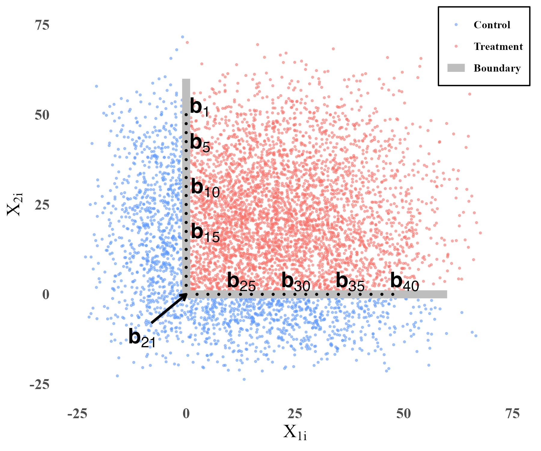
(a) Scatter Plot of $(X_{1i},X_{2i})$

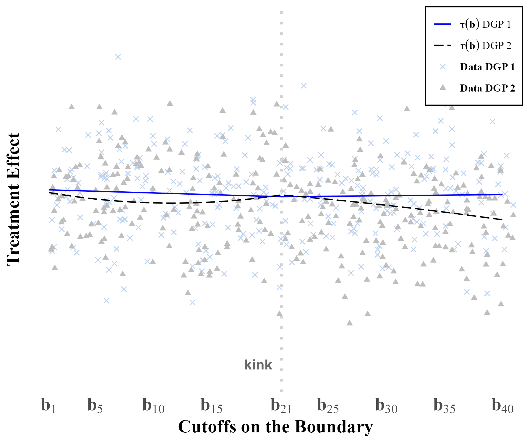
(b) Treatment Effects Along the Boundary

Figure 2: Estimation and Inference (Simulations).

3.1 Function rd2d()

The function rd2d() provides point estimation, robust confidence intervals, and robust uniform confidence bands for (derivatives of) treatment effect function $\tau(\mathbf{x})$ based on bivariate location-based local polynomial regression. It takes as input an outcome vector y, a bivariate location score matrix X, a treatment indicator vector t, and a grid of evaluation points b along the boundary $\mathcal{B}$.

Optional arguments include bandwidth choices h, degrees of polynomial for point estimation (p) and inference (q), the partial derivative of treatment effect to be estimated deriv, and confidence level level. When optional arguments are not provided, the function defaults to estimate the value of treatment effect deriv = c(0,0) using the MSE-optimal bandwidth, with p = 1 degree polynomial for point estimation and q = 2 degree polynomial for robust bias-corrected confidence interval (and bands if requested), and level = 95 percentage points confidence level. Additionally, kernel_type indicates whether a product kernel ("prod") or a radial kernel ("rad") is used for weighting. The default is kernel_type = "prod".

Below is a demonstration of rd2d() applied on the synthetic dataset, with results for selected indices printed using the summary() method.

⬇

> result.rd2d <- rd2d(y, X, t, eval)

> summary(result.rd2d, subset = c(1,5,10,15,21,25,30,35,40))

rd2d

Number of Obs. 20000

BW type. mserd-dpi-std

Kernel triangular-prod

VCE method hc1

Masspoints check

Number of Obs. 6191 13809

Estimand (deriv) 0 0

Order est. (p) 1 1

Order rbc. (q) 2 2

Unique Obs. 6191 13809

====================================================================

ID b1 b2 Est. z P>|z| 95% CI

====================================================================

1 0.000 50.000 0.8185 10.7556 0.0000 [0.6352, 0.9183]

5 0.000 40.000 0.7275 13.1931 0.0000 [0.6212, 0.8380]

10 0.000 27.500 0.6760 13.0532 0.0000 [0.5676, 0.7682]

15 0.000 15.000 0.6460 14.1746 0.0000 [0.5534, 0.7310]

21 0.000 0.000 0.6931 10.2638 0.0000 [0.5443, 0.8013]

25 10.000 0.000 0.6652 15.5194 0.0000 [0.5601, 0.7220]

30 22.500 0.000 0.6112 12.3397 0.0000 [0.5125, 0.7060]

35 35.000 0.000 0.5769 9.3480 0.0000 [0.4276, 0.6545]

40 47.500 0.000 0.5176 6.8977 0.0000 [0.3482, 0.6247]

====================================================================

Listing 1: Functionality of rd2d()

The first part of the output provides basic information on the options specified in the function. For example, the default estimand is the value of treatment effect, indicated by deriv = (0,0). The rest of the output gives estimation results, including (i) b1 and b2: First and second coordinate of the evaluation points; (ii) Coef.: Point estimation of (derivative) of treatment effect using $p=$ p polynomial order; and (iii) t-statistics, (iv) p-value, and (v) level% confidence intervals using $q=$ q polynomial order. When $q>p$, the resulting inference procedures correspond to robust bias correction (Calonico et al., 2014, 2018, 2022), which is the default and recommended method; $p=q$ corresponds to standard least squares methods. Point estimates, standard errors, and other information can be easily extracted for further statistical analysis. The output is stored in a standard matrix, and can be accessed with the following command,

⬇

> result.rd2d$main

> result.rd2d$main.A0

> result.rd2d$main.A1

Listing 2: Output matrices of rd2d()

where result.rd2d$main.A0 contains results for the control group, result.rd2d$main.A1 contains results for the treatment group, and result.rd2d$main contains results for both.

The summary() method allows for three optional arguments. First, the option subset takes the indices of evaluation points to be presented, which should be a subset of c(1:nrow(eval)). The default is NULL, and thus all evaluation points are presented. Second, CBuniform is boolean variable for confidence bands construction, where FALSE indicates that pointwise confidence intervals are provided, and TRUE indicates uniform confidence bands are provided. The default is CBuniform = FALSE.

⬇

> summary(result.rd2d, subset = c(1,5,10,15,21,25,30,35,40), CBuniform = TRUE)

rd2d

Number of Obs. 20000

BW type. mserd-dpi-std

Kernel triangular-prod

VCE method hc1

Masspoints check

Number of Obs. 6191 13809

Estimand (deriv) 0 0

Order est. (p) 1 1

Order rbc. (q) 2 2

Unique Obs. 6191 13809

====================================================================

ID b1 b2 Est. z P>|z| 95% Unif. CB

====================================================================

1 0.000 50.000 0.8185 10.7556 0.0000 [0.5593, 0.9942]

5 0.000 40.000 0.7275 13.1931 0.0000 [0.5631, 0.8961]

10 0.000 27.500 0.6760 13.0532 0.0000 [0.5138, 0.8220]

15 0.000 15.000 0.6460 14.1746 0.0000 [0.5058, 0.7786]

21 0.000 0.000 0.6931 10.2638 0.0000 [0.4754, 0.8702]

25 10.000 0.000 0.6652 15.5194 0.0000 [0.5166, 0.7654]

30 22.500 0.000 0.6112 12.3397 0.0000 [0.4606, 0.7579]

35 35.000 0.000 0.5769 9.3480 0.0000 [0.3667, 0.7153]

40 47.500 0.000 0.5176 6.8977 0.0000 [0.2741, 0.6988]

====================================================================

Listing 3: Functionality of rd2d() with CBuniform = TRUE

Finally, the summary() method allows for presenting the underlying bandwidths used and associated effective sample sizes via the option output = "bw".

⬇

> summary(result.rd2d, subset = c(1,5,10,15,21,25,30,35,40), output = "bw")

rd2d

Number of Obs. 20000

BW type. mserd-dpi-std

Kernel triangular-prod

VCE method hc1

Masspoints check

Number of Obs. 6191 13809

Estimand (deriv) 0 0

Order est. (p) 1 1

Order rbc. (q) 2 2

Unique Obs. 6191 13809

====================================================================

Bdy Points BW Control BW Treatment Eff. N

ID b1 b2 h01 h02 h11 h12 Nh0 Nh1

====================================================================

1 0.000 50.000 18.511 18.544 18.511 18.544 775 1650

5 0.000 40.000 16.679 16.709 16.679 16.709 1199 2322

10 0.000 27.500 14.352 14.378 14.352 14.378 1482 2693

15 0.000 15.000 12.690 12.713 12.690 12.713 1403 2381

21 0.000 0.000 16.778 16.808 16.778 16.808 2595 2098

25 10.000 0.000 13.587 13.611 13.587 13.611 1706 2303

30 22.500 0.000 12.206 12.228 12.206 12.228 1236 2095

35 35.000 0.000 12.492 12.514 12.492 12.514 919 1675

40 47.500 0.000 16.748 16.778 16.748 16.778 766 1562

====================================================================

Listing 4: Functionality of rd2d() with output = "bw"

3.2 Function rdbw2d()

The function rdbw2d() is used for MSE (or IMSE) optimal bandwidth implementation, and is used internally in rd2d() when user does not specify bandwidth choices manually. The function takes the same input data as rd2d(), that is, an outcome vector y, a bivariate location score matrix X, a treatment indicator vector t, and a grid of evaluation points b along the boundary $\mathcal{B}$. In addition, the option bwselect encodes four options of bandwidth type: (i) "mserd" finds the MSE-optimal bandwidth for estimating (derivatives of) treatment effect, (ii) "imserd" finds the integreated MSE optimal bandwidth for estimating (derivatives of) treatment effect, (iii) "msetwo" finds the MSE optimal bandwidth for estimation (the derivatives of) conditional means of two potential outcome variables, (iv) "imsetwo" finds the integrated MSE optimal bandwidth for estimation (the derivatives of) conditional means of two potential outcome variables. The default is bwselect = "mserd". An additional Boolean argument stdvar indicates whether the covariates are first standardized to unit standard deviation in each coordinate, in which case the optimal bandwidth is estimated and then converted back to the original scale. The default is stdvar = FALSE.

⬇

> bws.rd2d <- rdbw2d(y, X, t, eval)

> summary(bws.rd2d,subset = c(1,5,10,15,21,25,30,35,40))

Call: rdbw2d

Number of Obs. 20000

BW type. mserd-dpi

Kernel triangular-prod

VCE method hc1

Masspoints check

Standardization off

Number of Obs. 6191 13809

Estimand (deriv) 0 0

Order est. (p) 1 1

Unique Obs. 6191 13809

Bandwidth Selection

====================================================

Bdy Points BW Control BW Treatment

ID b1 b2 h01 h02 h11 h12

====================================================

1 0.000 50.000 22.719 22.719 22.719 22.719

5 0.000 40.000 21.253 21.253 21.253 21.253

10 0.000 27.500 18.355 18.355 18.355 18.355

15 0.000 15.000 14.514 14.514 14.514 14.514

21 0.000 0.000 21.382 21.382 21.382 21.382

25 10.000 0.000 16.965 16.965 16.965 16.965

30 22.500 0.000 13.772 13.772 13.772 13.772

35 35.000 0.000 14.683 14.683 14.683 14.683

40 47.500 0.000 21.170 21.170 21.170 21.170

====================================================

Listing 5: Functionality of rdbw2d()

The first part of the summary output lists the options used for bandwidth selection. The second part of the summary output gives bandwidth selection results, including: (i) Boundary points, b1 for the first coordinate and b2 for the second coordinate; (ii) Bandwidths for control group, h01 for the first coordinate and h02 for the second coordinate; (iii) Bandwidths for treatment group, h11 for the first coordinate and h12 for the second coordinate.

3.3 Function rd2d.dist()

The function rd2d.dist() provides point estimation and inference for boundary treatment effects using distance-based univariate local polynomial regression. It takes as input an outcome vector y, and a signed distance matrix D of distance to each boundary point, where each column of D corresponds to the signed distance from all observations to one evaluation point, with a positive sign indicating the unit is in the treatment group and a negative sign indicating the unit is in the control group.

Optional arguments include evaluation points b, bandwidth choices h, degrees of polynomial for point estimation (p) and inference (q), option for kink adjustment kink, and confidence level level, among other options. When not provided, the function defaults to estimate the value of treatment effect using the MSE-optimal bandwidth without kink adjustment (kink = "off"), using p = 1 degree polynomial for point estimation and q = 2 degree polynomial for robust bias-corrected confidence intervals and bands, providing level = 95% confidence interval and uniform confidence bands, and without displaying of evaluation points (b = NULL).

⬇

> result.dist <- rd2d.dist(y, D, b = eval)

> summary(result.dist, subset = c(1,5,10,15,21,25,30,35,40))

rd2d.dist

Number of Obs. 20000

BW type mserd-rot

Kernel triangular-rad

VCE method hc1

Masspoints check

Number of Obs. 6191 13809

Estimand (deriv) 0 0

Order est. (p) 1 1

Order rbc. (q) 2 2

====================================================================

ID b1 b2 Est. z P > |z| 95% CI

====================================================================

1 0.000 50.000 0.8371 11.5847 0.0000 [0.6515, 0.9166]

5 0.000 40.000 0.7307 9.4650 0.0000 [0.5808, 0.8839]

10 0.000 27.500 0.6572 9.7763 0.0000 [0.5124, 0.7691]

15 0.000 15.000 0.6272 7.7001 0.0000 [0.4345, 0.7309]

21 0.000 0.000 0.7426 6.8180 0.0000 [0.5059, 0.9134]

25 10.000 0.000 0.6301 11.2414 0.0000 [0.5474, 0.7785]

30 22.500 0.000 0.6109 7.3862 0.0000 [0.4338, 0.7469]

35 35.000 0.000 0.5768 6.4730 0.0000 [0.3670, 0.6853]

40 47.500 0.000 0.4654 6.7582 0.0000 [0.3603, 0.6543]

====================================================================

Listing 6: Functionality of rd2d.dist()

The first part of the summary output provides basic information on the options specified in the function. The rest of the summary output gives estimation and inference results, including: (i) b1 and b2 (when b is provided) report first and second coordinates of the evaluation points; (ii) Coef. reports the treatment effect estimate using a $p$th order polynomial regression; and (iii) the last three columns correspond to t-statistic, p-value and level% confidence intervals using $q$th order polynomial regression. The summary() method also has the option of displaying the uniform confidence bands (instead of the confidence intervals) in the last two columns as follows (numerical results omitted to conserve space).

⬇

> summary(result.dist, subset = c(1,5,10,15,21,25,30,35,40), CBuniform = TRUE)

Listing 7: Functionality of rd2d.dist() with CBuniform = TRUE

In addition, The summary() method can also display the underlying bandwidths and effective samples sizes as follows (numerical results omitted to conserve space).

⬇

> summary(result.dist, subset = c(1,5,10,15,21,25,30,35,40), output = "bw")

Listing 8: Functionality of rd2d.dist() with output = "bw"

Point estimates, standard errors, and other information can be easily extracted for further statistical analysis. The output is stored in a standard matrix, and can be accessed with the following command.

⬇

> result.dist$main

> result.dist$main.A0

> result.dist$main.A1

Listing 9: Output matrices of rd2d.dist()

result.dist$main.A0 contains results for the control group, result.dist$main.A1 contains results for the treatment group, and result.dist$main contains results for both.

3.4 Function rdbw2d.dist()

The function rdbw2d.dist() is used to implement MSE (or IMSE) rate-optimal ROT bandwidth selectors, and is used internally in rd2d.dist() when user does not provide bandwidths manually. As for rdbw2d(), four bandwidth types are allowed, that is, bwselect can be "mserd", "imserd", "msetwo" or "imsetwo".

⬇

> bws.dist <- rdbw2d.dist(y, D, b = eval)

> summary(bws.dist,subset = c(1,5,10,15,21,25,30,35,40))

Call: rdbw2d.dist

Number of Obs. 20000

BW type mserd-rot

Kernel triangular-rad

Kink off

VCE method hc1

Masspoints check

Number of Obs. 6191 13809

Estimand (deriv) 0 0

Order est. (p) 1 1

Bandwidth Selection

================================================

Bdy Points BW Control BW Treatment

ID b1 b2 h0 h1

================================================

1 0.000 50.000 32.918 32.918

5 0.000 40.000 22.071 22.071

10 0.000 27.500 20.899 20.899

15 0.000 15.000 14.455 14.455

21 0.000 0.000 14.381 14.381

25 10.000 0.000 19.712 19.712

30 22.500 0.000 14.041 14.041

35 35.000 0.000 16.722 16.722

40 47.500 0.000 27.499 27.499

================================================

Listing 10: Functionality of rdbw2d.dist()

An additional argument kink, taking values "off" or "on", indicates whether a kink adjustment is made for estimation and inference. The default is kink = "off", but when kink = "on" is specified then the bandwidth is shrank to account for lack of smoothness of the assignment boundary $\mathcal{B}$.

⬇

> bws.dist <- rdbw2d.dist(y, D, kink = "on")

> summary(bws.dist,subset = c(1,5,10,15,21,25,30,35,40))

Call: rdbw2d.dist

Number of Obs. 20000

BW type mserd-rot

Kernel triangular-rad

Kink on

VCE method hc1

Masspoints check

Number of Obs. 6191 13809

Estimand (deriv) 0 0

Order est. (p) 1 1

Bandwidth Selection

================================

BW Control BW Treatment

ID h0 h1

================================

1 14.421 14.421

5 9.670 9.670

10 9.156 9.156

15 6.333 6.333

21 6.300 6.300

25 8.636 8.636

30 6.152 6.152

35 7.326 7.326

40 12.048 12.048

================================

Listing 11: Functionality of rdbw2d.dist() with kink = "on"

3.5 Graphical Presentation

The package rd2d provides an array of estimation and inference results that can be used for graphical presentation. Figure 3(a) compares three point estimation methods: (i) bivariate method via rd2d; (ii) distance-based method via rd2d.dist, ignoring the kink (default argument kink = "off"); and (iii) distance-based method via rd2d.dist, adjusting for kink (kink = "on"). Figure 3(b) plots point estimation using the bivariate method, along with its associated robust bias-corrected confidence intervals and confidence band. Figure 3(c) presents a heatmap of treatment effects along the boundary, with high to low point estimation indicated by red to blue colors. Finally, Figure 3(d) presents a heatmap of p-values along the boundary, with five colors assigned to five ranges of values. The codes for generating the graphical presentations are given in the replication R file.

It can be seen that distance-based estimation with kink = "off" overshoots compared to the bivariate estimation before the kink, and undershoots after the kink. This corresponds to the phenomena of getting a first-order bias using distance based method in the presence of a kink, despite using local polynomial regression of degree greater than or equal to $1$. See Cattaneo et al. (2025) for more methodological and theoretical discussions.

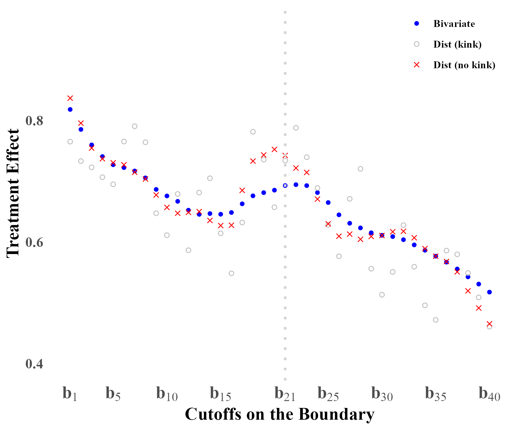
(a) Point Estimation

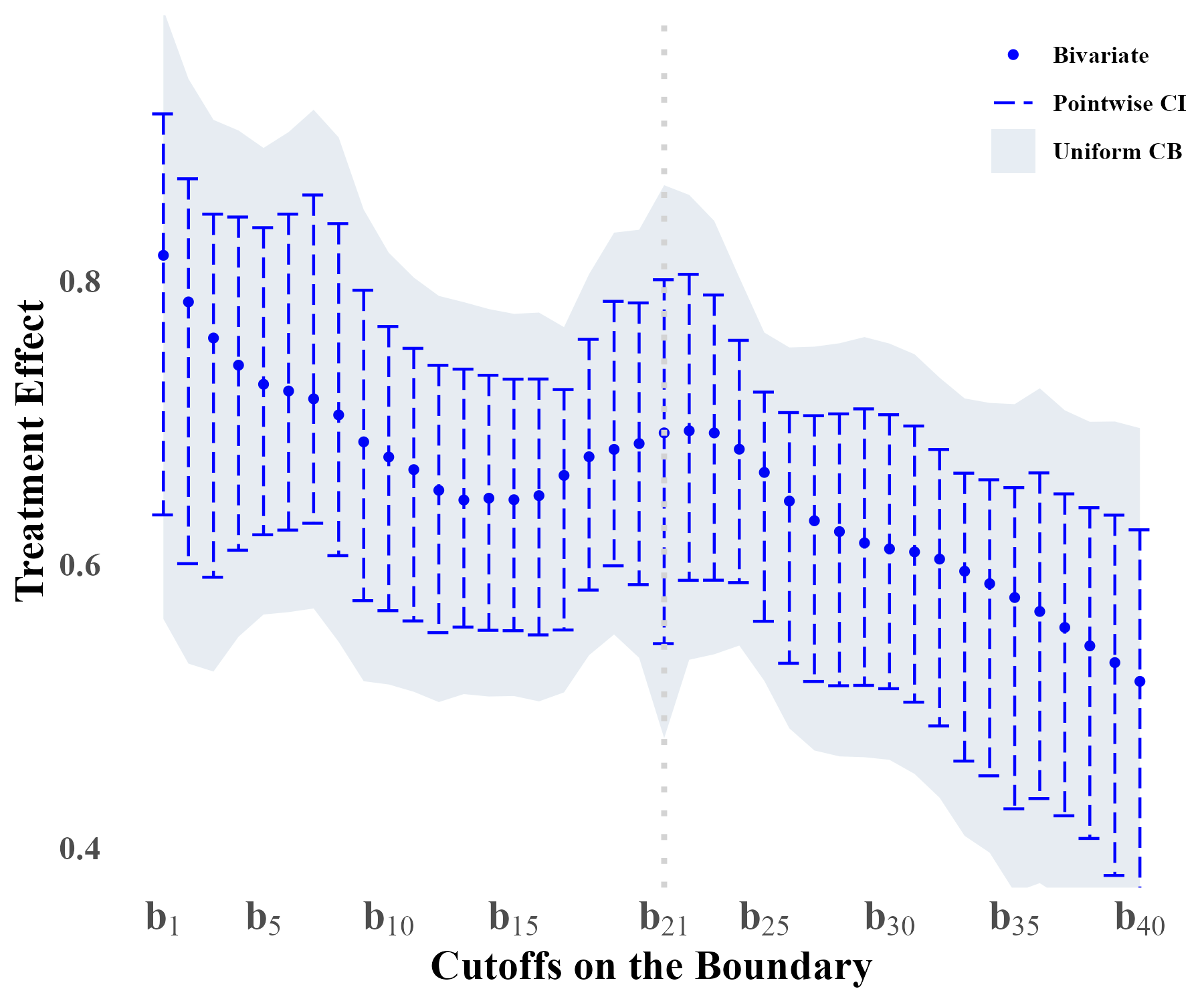
(b) Confidence Interval and Bands

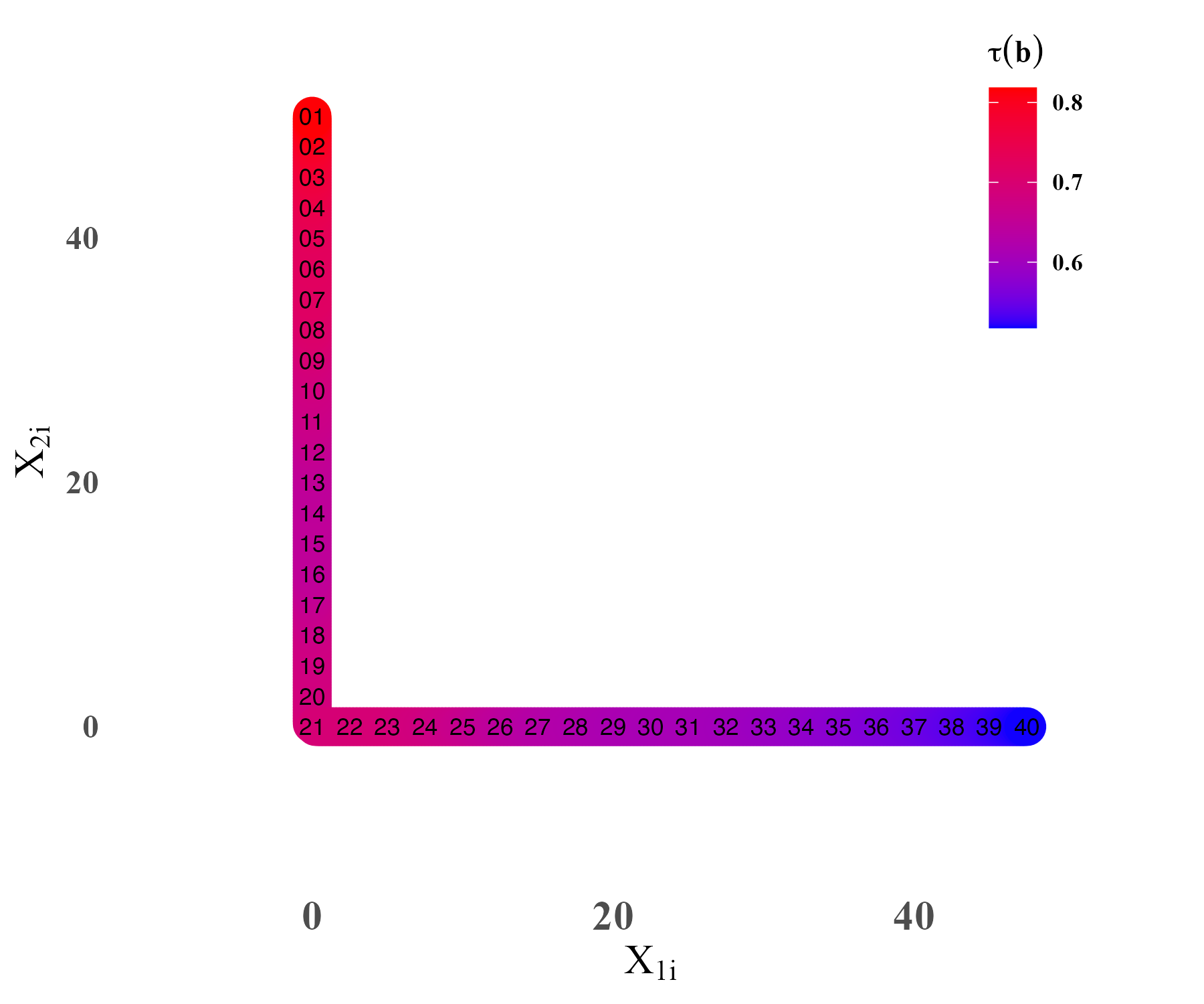
(c) Treatment Effects Heatmap

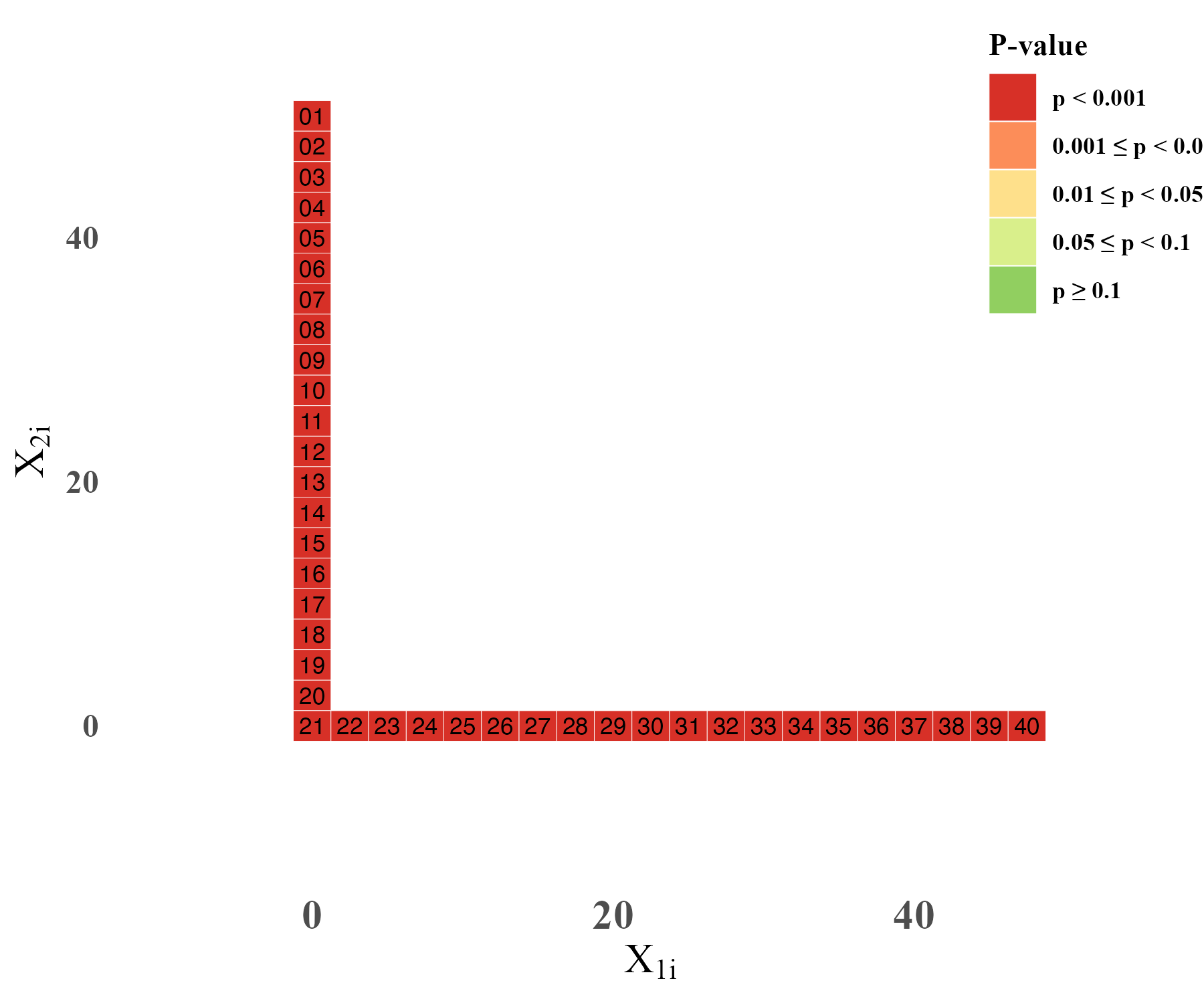
(d) p-values Heatmap

Figure 3: Estimation and Inference (Simulations).

3.6 Simulation Evidence

The discussion so far employed one realization of the data generating process to illustrate the main features of the package rd2d. In this final section, we conduct a Monte Carlo experiment to assess the performance of the package in repeated sampling. We consider $m=1,000$ simulations of the two data generating processes defined at the beginning of this section, and report the simulation results in Table 2 (DGP 1: linear model) and Table 3 (DGP 2: quadratic model). Three methods are used and compared: the bivariate method rd2d, the distance-based method rd2d.dist ignoring the presence of the kink in the boundary (kink = "off"), and the distance-based method rd2d.dist adjusting for the kink (kink = "on"). Bandwidths are chosen automatically by the package, and their average across simulations is reported. We also report diagnostic measures including: bias, standard deviation of point estimator, root mean-squared error of point estimator, pointwise empirical coverage, pointwise interval length, uniform empirical coverage, and uniform interval length.

For both DPG 1 and DGP 2, all of the three methods give pointwise coverage around 95%, while the pointwise interval length for rd2d and rd2d.dist (kink = "off") are smaller compared to rd2d.dist (kink = "on"). This is likely due to bandwidth shrinkage for kink adjustment, which does results in a significantly smaller bias compared to the one ignoring the kink. Both rd2d and rd2d.dist (kink = "off") give around 95% uniform coverage and a relatively shorter interval length compared to rd2d.dist (kink = "on"), likely due to the same reason.

Method	Index	$h$	Bias	SD	RMSE	EC	IL
rd2d	1	17.497	-0.000	0.049	0.049	0.942	0.287
	5	15.504	0.001	0.037	0.037	0.953	0.220
	10	13.399	0.002	0.035	0.035	0.945	0.197
	15	13.932	-0.000	0.031	0.031	0.947	0.175
	21	15.490	0.002	0.043	0.043	0.962	0.292
	25	13.964	-0.001	0.028	0.028	0.951	0.163
	30	13.146	-0.000	0.033	0.033	0.959	0.190
	35	14.536	0.002	0.036	0.036	0.954	0.207
	40	16.961	0.000	0.046	0.046	0.949	0.264
	Uniform					0.937	0.313
rd2d.dist kink = "off"	1	34.255	0.030	0.037	0.047	0.950	0.258
	5	26.741	0.015	0.036	0.039	0.955	0.240
	10	19.566	0.003	0.034	0.034	0.956	0.257
	15	16.968	0.002	0.038	0.038	0.955	0.271
	21	21.218	0.003	0.040	0.040	0.952	0.280
	25	18.707	-0.024	0.038	0.045	0.957	0.251
	30	16.976	0.001	0.037	0.037	0.957	0.279
	35	24.519	-0.005	0.034	0.034	0.939	0.233
	40	33.199	-0.014	0.036	0.039	0.952	0.243
	Uniform					0.951	0.407
rd2d.dist kink = "on"	1	15.007	0.009	0.075	0.075	0.954	0.674
	5	11.715	0.004	0.072	0.072	0.933	0.611
	10	8.572	-0.002	0.075	0.075	0.935	0.655
	15	7.434	-0.002	0.080	0.080	0.923	0.691
	21	9.296	0.004	0.087	0.087	0.924	0.738
	25	8.196	-0.002	0.074	0.074	0.928	0.645
	30	7.437	0.001	0.081	0.081	0.947	0.714
	35	10.742	0.002	0.071	0.071	0.945	0.593
	40	14.545	-0.001	0.074	0.074	0.950	0.632
	Uniform					0.877	1.071

Table 2: Simulation results for DGP 1 (Linear)

Method	Index	$h$	Bias	SD	RMSE	EC	IL
rd2d	1	17.329	0.006	0.048	0.048	0.953	0.289
	5	15.394	0.006	0.036	0.037	0.964	0.220
	10	13.339	0.004	0.034	0.034	0.943	0.197
	15	13.789	0.004	0.030	0.030	0.953	0.177
	21	15.194	-0.010	0.045	0.046	0.952	0.297
	25	13.954	-0.006	0.028	0.029	0.958	0.164
	30	13.086	-0.003	0.033	0.033	0.950	0.192
	35	14.511	-0.003	0.036	0.036	0.950	0.206
	40	16.851	-0.004	0.046	0.046	0.943	0.264
	Uniform					0.953	0.315
rd2d.dist kink = "off"	1	34.144	0.039	0.038	0.055	0.927	0.259
	5	24.612	0.016	0.039	0.042	0.942	0.260
	10	18.392	0.002	0.037	0.037	0.948	0.271
	15	14.216	-0.002	0.042	0.042	0.957	0.320
	21	21.137	-0.005	0.038	0.039	0.956	0.282
	25	16.227	-0.025	0.045	0.052	0.950	0.288
	30	13.810	-0.004	0.047	0.047	0.944	0.337
	35	19.163	-0.019	0.045	0.048	0.927	0.294
	40	31.515	-0.070	0.041	0.082	0.946	0.259
	Uniform					0.948	0.460
rd2d.dist kink = "on"	1	14.959	0.017	0.081	0.083	0.942	0.677
	5	10.783	0.001	0.079	0.079	0.940	0.663
	10	8.058	0.003	0.082	0.082	0.942	0.691
	15	6.228	-0.001	0.095	0.095	0.919	0.821
	21	9.260	-0.001	0.085	0.085	0.924	0.749
	25	7.109	-0.000	0.088	0.088	0.917	0.734
	30	6.050	-0.003	0.104	0.104	0.916	0.840
	35	8.395	-0.003	0.089	0.089	0.924	0.754
	40	13.807	-0.017	0.078	0.079	0.943	0.664
	Uniform					0.846	1.197

Table 3: Simulation results for DGP 2 (Quadratic)

4 Conclusion

This paper introduced the R software package rd2d for causal inference in Boundary Discontinuity designs. The package provides pointwise and uniform (over the treatment assignment boundary) estimation and inference methods employing either a bivariate location score or a univariate distance score. In addition, the methods can be used for graphical presentation. From a methodological perspective, this paper introduced second generation bandwidth selection methods complementing the main results in Cattaneo et al. (2025). Simulation evidence demonstrated a good performance of the package rd2d. Replication codes and related information are available at: https://rdpackages.github.io/rd2d/.

References

- Calonico et al. [2014] Sebastian Calonico, Matias D. Cattaneo, and Rocio Titiunik. Robust nonparametric confidence intervals for regression-discontinuity designs. Econometrica, 82(6):2295–2326, 2014.
- Calonico et al. [2018] Sebastian Calonico, Matias D. Cattaneo, and Max H. Farrell. On the effect of bias estimation on coverage accuracy in nonparametric inference. Journal of the American Statistical Association, 113(522):767–779, 2018.
- Calonico et al. [2022] Sebastian Calonico, Matias D. Cattaneo, and Max H. Farrell. Coverage error optimal confidence intervals for local polynomial regression. Bernoulli, 28(4):2998–3022, 2022.
- Cattaneo and Titiunik [2022] Matias D. Cattaneo and Rocio Titiunik. Regression discontinuity designs. Annual Review of Economics, 14:821–851, 2022.
- Cattaneo et al. [2020] Matias D. Cattaneo, Nicolás Idrobo, and Rocio Titiunik. A Practical Introduction to Regression Discontinuity Designs: Foundations. Cambridge University Press, 2020.
- Cattaneo et al. [2024] Matias D. Cattaneo, Nicolás Idrobo, and Rocio Titiunik. A Practical Introduction to Regression Discontinuity Designs: Extensions. Cambridge University Press, 2024.
- Cattaneo et al. [2025] Matias D Cattaneo, Rocio Titiunik, and Ruiqi Rae Yu. Estimation and inference in boundary discontinuity designs. arXiv preprint arXiv:2505.05670, 2025.
- Hahn et al. [2001] Jinyong Hahn, Petra Todd, and Wilbert van der Klaauw. Identification and estimation of treatment effects with a regression-discontinuity design. Econometrica, 69(1):201–209, 2001.
- Härdle et al. [2004] Wolfgang Härdle, Marlene Müller, Stefan Sperlich, Axel Werwatz, et al. Nonparametric and semiparametric models, volume 1. Springer, 2004.
- Jardim et al. [2024] Ekaterina Jardim, Mark C Long, Robert Plotnick, Jacob Vigdor, and Emma Wiles. Local minimum wage laws, boundary discontinuity methods, and policy spillovers. Journal of Public Economics, 234:105131, 2024.
- Keele and Titiunik [2015] Luke J. Keele and Rocio Titiunik. Geographic boundaries as regression discontinuities. Political Analysis, 23(1):127–155, 2015.
- Londoño-Vélez et al. [2020] Juliana Londoño-Vélez, Catherine Rodríguez, and Fabio Sánchez. Upstream and downstream impacts of college merit-based financial aid for low-income students: Ser pilo paga in colombia. American Economic Journal: Economic Policy, 12(2):193–227, 2020.
- Papay et al. [2011] John P Papay, John B Willett, and Richard J Murnane. Extending the regression-discontinuity approach to multiple assignment variables. Journal of Econometrics, 161(2):203–207, 2011.
- Reardon and Robinson [2012] Sean F Reardon and Joseph P Robinson. Regression discontinuity designs with multiple rating-score variables. Journal of Research on Educational Effectiveness, 5(1):83–104, 2012.
- Wand and Jones [1994] Matt P Wand and M Chris Jones. Kernel smoothing. CRC press, 1994.
- Zeileis [2004] Achim Zeileis. Econometric computing with hc and hac covariance matrix estimators. Journal of Statistical Software, 11(10):1–17, 2004.
- Zeileis et al. [2020] Achim Zeileis, Susanne Köll, and Nathaniel Graham. Various versatile variances: An object-oriented implementation of clustered covariances in r. Journal of Statistical Software, 95:1–36, 2020.