Disparity in sound speeds: implications for unitarity and effective potential in quantum field theory

Abstract

We develop a complete unitarity framework for quantum field theories whose massive scalar excitations propagate at different sound speeds. Starting from first principles we derive the exact partial-wave unitarity condition for $2\rightarrow 2$ scattering with arbitrary masses and velocity hierarchies, recovering the standard and massless limits as special cases. Applying the formalism to a renormalizable two-field model we verify the optical theorem at one loop and obtain compact, velocity-dependent perturbative unitarity bounds.

Then we compute the one-loop Coleman-Weinberg potential in the background-field method, tracking how a small splitting between sound speeds reshapes the renormalization-group flow. We find that all of quartic $\beta$-functions are rescaled in such a way that an accidental fixed line emerges.

1 Introduction

Probability conservation, embodied in the unitarity of the $S$-matrix, has long been one of the most powerful consistency checks on quantum field theories (QFTs). Its quantitative incarnation—the partial-wave unitarity relation—has famously constrained the Higgs-boson mass Lee:1977yc ; Lee:1977eg , guided model building in strongly-interacting electroweak sectors Chanowitz:1985hj , general aspects of quantum field theory Corbett:2014ora and continues to shape modern effective-field-theory (EFT) analyses of hadronic, electroweak and gravitational processes Oller:2019opk ; Baumgart:2022yty . Unitarity relation and partial wave expansions Oller:2019opk ; oller.190503.1 ; Lacour:2009ej ; Gulmez:2016scm are fundamental tools for ensuring probability (i.e. unitarity) conservation and analyzing angular momentum contributions to the final physical answers. While most classic studies assume relativistic dispersion with a universal (unit) speed of light, many contemporary frameworks—from multi-field inflation to Lorentz-violating extensions of the Standard Model—harbour scalar degrees of freedom that propagate with different sound speeds. Moreover it is known the scalar perturbations of single- and multi-field inflation (and not only inflation) generically propagate with reduced or field-dependent sound speeds Cheung:2007st ; Armendariz-Picon:1999hyi ; Garriga:1999vw ; Alishahiha:2004eh ; Kobayashi:2010cm ; Kobayashi:2011nu ; Creminelli:2010ba ; Hinterbichler:2012fr ; Pirtskhalava:2014esa ; Nishi:2015pta ; Kobayashi:2015gga ; Kolevatov:2017voe ; Qiu:2011cy ; Easson:2011zy ; Cai:2012va ; Osipov:2013ssa ; Qiu:2013eoa ; Koehn:2013upa ; Qiu:2015nha ; Ijjas:2016tpn ; Mironov:2018oec ; Ageeva:2022asq . Anisotropic scaling appears in Hořava–Lifshitz gravity Horava:2009uw and in some extensions of the Standard Model Myers:2003fd . Coupled-channel analyses routinely rely on partial-wave unitarity to constrain amplitudes and extract resonance properties Oller:2019opk . Such anisotropic kinematics dramatically alters both dispersion relations and the algebraic structure of the unitarity condition. A systematic treatment of unitarity in this broader setting, including the massive case, is therefore essential.

Motivated by these developments we revisit $2\to 2$ scattering in theories of real scalars $\phi_{i}$ with distinct propagation velocities $u_{i}$ and arbitrary masses $m_{i}$. We extend the results of Ageeva:2022byg and derive the exact unitarity relation for partial-wave amplitudes when all external and internal particles carry generic masses and sound speeds, then check the result explicitly in a renormalizable two-field model, and extract the resulting perturbative unitarity bounds. Compared with the massless case the presence of non-zero $m_{i}$ introduces a non-trivial interplay between Lorentz-breaking kinematics and threshold behaviour, leading to modified phase-space weights that survive even in the equal-speed limit $u_{1}=u_{2}$. Moreover, we present a brief sketch of what could happen (for instance, with the one loop matrix element) and which new coefficients one should obtain when considering fully anisotropic theory, i.e. with different sound speed component for each spatial dimension. We discuss interesting applications of such kind of model in Conclusion as well.

Unitarity constraints are only half of the story: any consistent EFT must also remain under perturbative control as one flows to higher energies. The one-loop (Coleman–Weinberg) effective potential Coleman:1973jx provides a convenient window on the renormalization-group (RG) evolution and vacuum stability of multi-scalar theories. Using the background-field method and dimensional regularization we compute corrections for the same two-field model, allowing for a small splitting $\delta=u_{2}-u_{1}$ in the sound speeds. Our result reproduces the canonical Coleman–Weinberg form when $\delta=0$ and reveals a simple overall rescaling of the RG $\beta$-functions, $\beta_{\lambda_{i}}\propto(c_{s}-\frac{3}{2}\delta)$, to leading order in $\delta$ (here $c_{s}$ is the smaller sound speed). Intriguingly, this implies an accidental fixed line at $\delta=\frac{2}{3}c_{s}$, along which the one-loop running of all quartic couplings vanishes. The renormalization in the presence of spatial anisotropy (in the spirit of our sound speed disparity) in quantum field theory has been previously considered in Arefeva:1994qr ; Periwal:1995wm .

The paper is organized as follows. A brief recap of common QFT formulas for the theory of several scalar massive fields all with different sound speeds and then the derivation of generalized unitarity relation and bound for massive case are given in Sec. 2. Sec. 3 illustrates that derived in Sec. 2 unitarity relation for massive fields holds for some chosen toy model in the leading order by coupling constants. Short Sec. 4 provides a sketch of how to generalize the found optical theorem from Sec. 2 to the case of anisotropic by all spatial dimensions sound speeds. Sec. 5 is dedicated to the evaluation of effective potential and beta functions in the model from Sec. 3. This paper includes Appendix A, where we collect the explicit calculations of imaginary part of considered one loop matrix elements.

2 Derivation of unitarity relation and bound for the case of massive fields

This Section is dedicated to the derivation of unitarity relation in the case of massive real scalar fields, which have different sound speeds. Taking into account all these properties (masses and sound speeds) modifies the dispersion relation as well as final answer for unitarity relation and unitarity bound. To begin with, we consider $2\to 2$ scattering processes in theory with fields $\phi_{i}$ whose sound speeds $u_{i}$ are different. Then the corresponding action reads

$$S=\sum_{i}S_{\phi_{i}}\;,\;\;\;\;S_{\phi_{i}}=\int d^{4}x\left(\frac{1}{2}\dot{\phi_{i}}^{2}-\frac{1}{2}u_{i}^{2}(\vec{\nabla}\phi_{i})^{2}-\frac{1}{2}m_{i}^{2}\phi_{i}^{2}\right),$$ (1)

and we work with the $(+,-,-,-)$ signature of the Minkowski space-time. The equation of motion for $\phi_{i}$ is

$$\ddot{\phi_{i}}-u_{i}^{2}\Delta\phi_{i}+m_{i}^{2}\phi_{i}=0,$$ (2)

whose solution reads

$$\phi_{i}(\vec{x},t)=\int\frac{d\vec{p}_{i}}{(2\pi)^{3}}\frac{1}{\sqrt{2E_{p_{i}}}}\Big{(}a_{\vec{p}_{i}}\text{e}^{-iE_{p_{i}}t+i\vec{p}_{i}\vec{x}}+a_{\vec{p}_{i}}^{\dagger}\text{e}^{iE_{p_{i}}t-i\vec{p}_{i}\vec{x}}\Big{)},$$ (3)

with

$$E^{2}_{p_{i}}=u_{i}^{2}p_{i}^{2}+m_{i}^{2}\;,$$ (4)

while the operators $a_{\vec{p}_{i}}$ and $a_{\vec{p}_{i}}^{\dagger}$ obey the standard commutation relation

$$[a_{\vec{p}_{i}^{\,\prime}},a_{\vec{p}_{j}}^{\dagger}]=(2\pi)^{3}\delta^{(3)}(\vec{p}_{i}^{\,\prime}-\vec{p}_{j})\delta_{ij}.$$ (5)

Next, define one-particle state as

$$\ket{\vec{p}_{i}\;}\equiv\sqrt{2E_{p_{i}}}a_{\vec{p}_{i}}^{\dagger}\ket{0},$$ (6)

so that

$$\braket{0|\phi_{i}(\vec{x},t)|\vec{p\,}_{j}}=\text{e}^{-iE_{p_{j}}t+i\vec{p}_{j}\vec{x}}\delta_{ij}\;.$$ (7)

The normalization of the latter reads

$$\braket{\vec{p\;}^{\prime}_{j}|\vec{p\;}_{i}}=(2\pi)^{3}\sqrt{2E_{p_{j}^{\prime}}2E_{p_{i}}}\delta^{(3)}(\vec{p}_{i}-\vec{p}_{j}^{\,\prime})\delta_{ij}.$$ (8)

and then the representation of unit element is

$$1=\int\frac{d^{3}p_{i}}{(2\pi)^{3}2E_{p_{i}}}\ket{\vec{p\;}_{i}}\bra{\vec{p\;}_{i}}.$$ (9)

Next step for our further purposes is to recall the definitions of $S$-matrix and $T$-matrix, which in its turn are related as:

$$S=1+iT.$$ (10)

The transfer matrix $T$ is connected with matrix element $M$ as:

$$T=(2\pi)^{4}\delta^{4}\big{(}\mathcal{P}^{\mu\,\prime}-\mathcal{P}^{\mu}\big{)}M\;,$$ (11)

where $\mathcal{P}^{\mu}=\sum p^{\mu}_{\text{in}}$ and $\mathcal{P}^{\mu\,\prime}=\sum p^{\mu}_{\text{out}}$ are total 4-momenta of the initial and final state, respectively.

It is convenient for the consideration of scattering processes to introduce an initial state as martin.290916.1

$$\ket{\psi,\beta}=\sqrt{2E_{p_{1}}}\sqrt{2E_{p_{2}}}a^{\dagger}_{p_{1}}a^{\dagger}_{p_{2}}\ket{0},$$ (12)

with two particles of momenta $\vec{p}_{1}$ and $\vec{p}_{2}$; and a final state $\ket{\psi^{\prime},\beta^{\prime}}$ with two particles of momenta $\vec{p}_{1}\,^{\prime}$ and $\vec{p}_{2}\,^{\prime}$. There $\beta$ refers to the types of the two particles, i.e. $\beta\equiv\{\phi_{i},\phi_{j}\}$, while notation $\psi$ is a shorthand for the pair of momenta, $\psi\equiv\{\vec{p}_{1},\vec{p}_{2}\}$. Thus, we also can write

$$\ket{\psi,\beta}=\ket{\phi_{i},\vec{p}_{1}}\otimes\ket{\phi_{j},\vec{p}_{2}}\;.$$

The two cases can be considered: distinguishable and identical particles in the pair $\beta=\{\phi_{i},\phi_{j}\}$. We start with the first option below.

2.1 Case of distinguishable particles

We start with the scalar product of $\ket{\psi^{\prime},\beta^{\prime}}$ and $\ket{\psi,\beta}$ states:

$$\braket{\psi^{\prime},\beta^{\prime}\;|\psi,\beta\;}=(2\pi)^{6}2E_{p_{1}}2E_{p_{2}}\delta^{(3)}(\vec{p}_{1}\;^{\prime}-\vec{p}_{1})\delta^{(3)}(\vec{p}_{2}\;^{\prime}-\vec{p}_{2})\delta_{\beta^{\prime}\beta}\;,$$ (13)

what comes from the normalization (8). Below we consider the center-of-mass frame (CM frame) for the system of two colliding particles. In CM frame we commonly denote:
(i) $\vec{p}\equiv\vec{p}_{1}=-\vec{p}_{2}$; (ii) $p\equiv|\vec{p}\;|=|\vec{p}_{1}|=|\vec{p}_{2}|$; (iii) $\hat{\vec{p}}\equiv\vec{p}/p$, i.e. the unit vector along $\vec{p}$ and $\theta,\phi$ are the corresponding polar and azimuthal angles, respectively. Since below we are going to use partial wave expansion, the first step to this formalism is to replace the variables $\vec{p}_{1}$, $\vec{p}_{2}$ in (13) by total momentum $\mathcal{P}^{\mu}\equiv p_{1}^{\mu}+p_{2}^{\mu}$, $\theta$ and $\phi$, where we bear in mind that in CM frame we can choose $\mathcal{P}^{\mu}\approx(E,0)$ with $E=E_{1}+E_{2}=\sqrt{u_{1}^{2}p^{2}+m_{1}^{2}}+\sqrt{u_{2}^{2}p^{2}+m_{2}^{2}}$ and we rename sound speeds a little as $u_{1\beta}\equiv u_{i}$, $u_{2\beta}\equiv u_{j}$ which are related to the type of particle in a pair $\beta=\{\phi_{i},\phi_{j}\}$. We find for the volume

$$d^{3}\vec{\mathcal{P}}p^{2}dpd\hat{\vec{p}}=d^{4}\mathcal{P}_{\mu}d\hat{\vec{p}}\frac{p\sqrt{(u_{1\beta}^{2}p^{2}+m_{1}^{2})(u_{2\beta}^{2}p^{2}+m_{2}^{2})}}{u^{2}_{1\beta}\sqrt{u_{2\beta}^{2}p^{2}+m_{2}^{2}}+u^{2}_{2\beta}\sqrt{u_{1\beta}^{2}p^{2}+m_{1}^{2}}},$$ (14)

and then also change the variables for the delta functions

$$\delta^{(3)}(\vec{p}_{1}\;^{\prime}-\vec{p}_{1})\delta^{(3)}(\vec{p}_{2}\;^{\prime}-\vec{p}_{2})\delta_{\beta\beta^{\prime}} =\frac{\Big{(}u^{2}_{1\beta}\sqrt{u_{2\beta}^{2}p^{2}+m_{2}^{2}}+u^{2}_{2\beta}\sqrt{u_{1\beta}^{2}p^{2}+m_{1}^{2}}\Big{)}}{p\sqrt{(u_{1\beta}^{2}p^{2}+m_{1}^{2})(u_{2\beta}^{2}p^{2}+m_{2}^{2})}}\times$$

$$\times\delta^{(4)}(\mathcal{P}_{\mu}^{\prime}-\mathcal{P}_{\mu})\delta^{(2)}(\hat{\vec{p}}\;^{\prime}-\hat{\vec{p}}\;)\delta_{\beta\beta^{\prime}},$$ (15)

thus, we finally arrive from (13) to

$$\langle\psi^{\prime},\beta^{\prime}|\psi,\beta\rangle=\frac{4(u_{1\beta}^{2}E_{2}+u_{2\beta}^{2}E_{1})}{p}(2\pi)^{6}\delta^{(4)}(\mathcal{P}^{\mu^{\prime}}-\mathcal{P}^{\mu})\delta^{(2)}(\hat{\vec{p}}\;^{\prime}-\hat{\vec{p}}\;)\delta_{\beta^{\prime}\beta},$$ (16)

where we use $E_{p_{1}}\equiv E_{1}=\sqrt{u_{1}^{2}p^{2}+m_{1}^{2}}$ and $E_{p_{2}}\equiv E_{2}=\sqrt{u_{2}^{2}p^{2}+m_{2}^{2}}$, since we work in CM frame. If we take massless limit ($m_{1}=m_{2}=0$) in the latter expression, then $E_{1}=u_{1\beta}p$, $E_{2}=u_{2\beta}p$, and $E=(u_{1\beta}+u_{2\beta})p$, so we obtain

$$\langle\psi^{\prime},\beta^{\prime}|\psi,\beta\rangle=(2\pi)^{6}4u_{1\beta}u_{2\beta}(u_{1\beta}+u_{2\beta})\delta^{(4)}(\mathcal{P}^{\mu^{\prime}}-\mathcal{P}^{\mu})\delta^{(2)}(\hat{\vec{p}}\;^{\prime}-\hat{\vec{p}}\;)\delta_{\beta^{\prime}\beta},$$ (17)

which matches the corresponding result from Ref. Ageeva:2022byg .

Since the unitarity relation has simple form for the partial-wave amplitudes (PWAs) Oller:2019opk ; oller.190503.1 ; Lacour:2009ej ; Gulmez:2016scm , we turn to this representation and to this end we introduce two-particle state of definite angular momentum in the CM frame:

$$\ket{l,m,\mathcal{P}^{\mu},\beta}=\frac{1}{\sqrt{4\pi}}\int d\hat{\vec{p}}\;Y^{m}_{l}(\hat{\vec{p}}\;)\ket{\psi\;,\beta}.$$ (18)

An integration in the latter formula runs over unit sphere; it is also helpful to recall that $Y^{m}_{l}$ (spherical functions)

$$Y^{m}_{l}(\hat{\vec{p}}\;)=(-1)^{\frac{|m|-m}{2}}\mbox{e}^{im\phi}\sqrt{\frac{(2l+1)}{4\pi}\frac{(l-|m|)!}{(l+|m|)!}}P_{l|m|}(\cos\theta)\;,$$ (19)

obey

$$\int d\hat{\vec{p}}\;Y^{m}_{l}(\hat{\vec{p\;}})Y^{m^{\prime}*}_{l^{\prime}}(\hat{\vec{p\;}})=\delta_{ll^{\prime}}\delta_{mm^{\prime}}\;.$$ (20)

Surely, these formulas (18)-(20) remain the same – no matter massive or massless case is under the consideration. Thus, the scalar product of these states reads:

$$\braket{l^{\prime},m^{\prime},\mathcal{P}^{\mu\,\prime},\beta^{\prime}|l,m,\mathcal{P}^{\mu},\beta}=\frac{4\pi(u_{1\beta}^{2}E_{2}+u_{2\beta}^{2}E_{1})}{p}(2\pi)^{4}\delta^{(4)}(\mathcal{P}^{\mu\,\prime}-\mathcal{P}^{\mu})\delta_{ll^{\prime}}\delta_{mm^{\prime}}\delta_{\beta\beta^{\prime}},$$ (21)

where we use (16) and the decomposition of the unit operator is

$$1=\int d^{4}\mathcal{P}\sum_{l,m,\beta}\ket{l,m,\mathcal{P}^{\mu},\beta}\bra{l,m,\mathcal{P}^{\mu},\beta}\frac{1}{N(\beta)}+\ldots,$$ (22)

with the summation running over all possible two-particle states and normalization factor is

$$N(\beta)\equiv 2(2\pi)^{5}\frac{\left(u_{1\beta}^{2}E_{2}+u_{2\beta}^{2}E_{1}\right)}{p}.$$ (23)

Dots in (22) stand for terms with multiparticle states; for now we omit these terms (see the corresponding discussion about omitting of multiparticle states contribution in Ref. Ageeva:2022byg ).

The partial wave amplitude is defined as

$$T^{(l)}_{m^{\prime}\beta^{\prime};{m}{\beta}}=\braket{l,m^{\prime},\mathcal{P}^{\mu\,\prime},\beta^{\prime}|T|l,m,\mathcal{P}^{\mu},\beta}$$

$$=\frac{1}{4\pi}\int d\hat{\vec{p}}\int d\hat{\vec{p}}\;^{\prime}\;Y^{m}_{l}(\hat{\vec{p}}\;)Y^{{m^{\prime}}\,*}_{l}(\hat{\vec{p}}\;^{\prime})\braket{\psi\;^{\prime},\beta^{\prime}|T|\psi,{\beta}}\;.$$ (24)

while the amplitude $a_{l}$ is (see Ref. Ageeva:2022byg for detailed derivation of $a_{l}$)

$$a_{l,\beta^{\prime}\beta}=\frac{1}{32\pi}\int d(\cos\gamma)\cdot P_{l}(\cos\gamma)M_{\beta^{\prime}\beta},$$ (25)

and related to $T^{(l)}_{m^{\prime}\beta^{\prime};{m}{\beta}}$ as

$$T^{(l)}_{m^{\prime}\beta^{\prime};{m}{\beta}}=16\pi\cdot(2\pi)^{4}\delta^{(4)}(\mathcal{P}^{\mu\,\prime}-\mathcal{P}^{\mu})\delta_{m^{\prime}{m}}\leavevmode\nobreak\ a_{l,\beta^{\prime}\beta}\;.$$ (26)

To derive the unitarity relation we recall the unitarity of $S$-matrix, i.e. $SS^{\dagger}=S^{\dagger}S=1$, what implies

$$T-T^{\dagger}=iTT^{\dagger}=iT^{\dagger}T\;.$$ (27)

Now insert unit operator (22) in the r.h.s. of (27) and find

$$-i\left(T^{(l)}_{m^{\prime}\beta^{\prime};{m}{\beta}}-T^{(l)\,*}_{m\beta;{m^{\prime}}{\beta^{\prime}}}\right)=\int d^{4}\mathcal{P}^{\prime\prime}\sum_{m^{\prime\prime},\beta^{\prime\prime}}\frac{1}{N(\beta^{\prime\prime})}T^{(l)}_{m^{\prime}\beta^{\prime};m^{\prime\prime}\beta^{\prime\prime}}T^{(l)\,*}_{m\beta;m^{\prime\prime}\beta^{\prime\prime}}.$$ (28)

Next, using (26) as well as (23), we obtain unitarity relation in terms of PWAs $a_{l}$:

$$-\frac{i}{2}\left(a_{l,\alpha\beta}-a^{*}_{l,\beta\alpha}\right)=\sum_{\gamma}\frac{2p_{\gamma}}{(E_{2}u^{2}_{1\gamma}+E_{1}u^{2}_{2\gamma})}a_{l,\alpha\gamma}a^{*}_{l,\beta\gamma},$$ (29)

where $u_{1\gamma}$ and $u_{2\gamma}$ are sound speeds of particles in the intermediate state $\gamma$. Here we also introduce the notation $p_{\gamma}$ which is related to energies as $E=E_{1}+E_{2}=\sqrt{u_{1\gamma}^{2}p_{\gamma}^{2}+m_{1}^{2}}+\sqrt{u_{2\gamma}^{2}p_{\gamma}^{2}+m_{2}^{2}}$. Assuming the time reversal invariance holds (and so $T^{(l)}_{m^{\prime}\beta^{\prime};{m}{\beta}}=T^{(l)}_{m\beta;{m^{\prime}}{\beta^{\prime}}}$ and hence $a_{l,\alpha\beta}=a_{l,\beta\alpha}$, see Refs. martin.290916.1 ; Oller:2018zts ), the latter formula (29) can be rewritten as

$$\text{Im}\leavevmode\nobreak\ a_{l,\alpha\beta}=\sum_{\gamma}\frac{2p_{\gamma}}{(E_{2}u^{2}_{1\gamma}+E_{1}u^{2}_{2\gamma})}a_{l,\alpha\gamma}a^{*}_{l,\beta\gamma}.$$ (30)

If one takes $u_{1\gamma}=u_{2\gamma}=1$, then this relation coincides with the standard one from, for instance, Refs. Oller:2019opk ; DeCurtis:2003zt , while in the case of massless particles this formula turns to the result of Ref. Ageeva:2022byg :

$$\text{Im}\leavevmode\nobreak\ a_{l,\alpha\beta}=\sum_{\gamma}\frac{2}{u_{1\gamma}u_{2\gamma}(u_{1\gamma}+u_{2\gamma})}a_{l,\alpha\gamma}a^{*}_{l,\gamma\beta}.$$ (31)

Below we turn to the identical particles case.

2.2 Case of identical particles

In this subsection we also begin with the two-particle state, which can be defined for identical particles in the pair as follows:

$$\ket{\psi,\beta}=\sqrt{2E_{p_{1}}}\sqrt{2E_{p_{2}}}a^{\dagger}_{p_{1}}a^{\dagger}_{p_{2}}\ket{0},$$ (32)

with $\beta=\{\phi_{i},\phi_{i}\}$. The commutation relation for operators above is given by (5) as well. The difference (in comparison with distinguishable particles) appears in the normalization of the two-particle state, which is now given by:

$$\braket{\psi^{\prime},\beta^{\prime}\;|\psi,\beta\;}$$

$$\leavevmode\nobreak\ \leavevmode\nobreak\ \leavevmode\nobreak\ =(2\pi)^{6}2E_{p_{1}}2E_{p_{2}}\Big{(}\delta^{(3)}(\vec{p}_{1}\;^{\prime}-\vec{p}_{1})\delta^{(3)}(\vec{p}_{2}\;^{\prime}-\vec{p}_{2})+\delta^{(3)}(\vec{p}_{2}\;^{\prime}-\vec{p}_{1})\delta^{(3)}(\vec{p}_{1}\;^{\prime}-\vec{p}_{2}\;)\Big{)}\delta_{\beta\beta^{\prime}},$$ (33)

so that we take into account (by adding one another term with pair of delta functions) that we can change particles in initial/final states since they are identical. The same change of variables in (2.2) as in previous subsection gives

$$\braket{\psi^{\prime},\beta^{\prime}\;|\psi,\beta\;}=(2\pi)^{6}\cdot 8u_{\beta}^{2}\frac{E_{p}}{p}\cdot\delta^{(4)}(\mathcal{P}^{\mu\,\prime}-\mathcal{P}^{\mu})\Big{(}\delta^{(2)}(\hat{\vec{p}}\;^{\prime}-\hat{\vec{p}})+\delta^{(2)}(\hat{\vec{p}}\;^{\prime}+\hat{\vec{p}})\Big{)}\delta_{\beta\beta^{\prime}},$$ (34)

where $u_{\beta}\equiv u_{i}$ is the sound speed of the particle $\phi_{i}$ and $E_{p}=\sqrt{u^{2}_{\beta}p^{2}+m_{\beta}^{2}}$ with $m_{\beta}$ being the mass of $\phi_{i}$. The scalar product of definite angular momentum states is now

$$\braket{l^{\prime},m^{\prime},\mathcal{P}^{\mu\,\prime},\beta^{\prime}|l,m,\mathcal{P}^{\mu},\beta}=\frac{1}{4\pi}\int d\hat{\vec{p}}\;(2\pi)^{2} \cdot 8u_{\beta}^{2}\frac{E_{p}}{p}\cdot(2\pi)^{4}\delta^{(4)}(\mathcal{P}^{\mu\,\prime}-\mathcal{P}^{\mu})\delta_{\beta\beta^{\prime}}$$

$$\times\Big{(}Y^{m}_{l}(\hat{\vec{p}})Y^{m^{\prime}*}_{l^{\prime}}(\hat{\vec{p}})+Y^{m}_{l}(\hat{\vec{p}})Y^{m^{\prime}*}_{l^{\prime}}(-\hat{\vec{p}})\Big{)}\;.$$ (35)

Since identical scalars always have even $l$ (the integral in the right hand side of (35) vanishes for odd $l$), we stick to even $l$ in this subsection. Making use of the property  (20) and

$$Y_{l}^{m}(-\hat{\vec{p}}) =(-1)^{l}\,Y_{l}^{m}(\hat{\vec{p}}),$$ (36)

we get

$$\braket{l^{\prime},m^{\prime},\mathcal{P}^{\mu\,\prime},\beta^{\prime}|l,m,\mathcal{P}^{\mu},\beta} =\;2\pi\cdot 8u_{\beta}^{2}\frac{E_{p}}{p}\cdot(2\pi)^{4}\delta^{(4)}(\mathcal{P}^{\mu\,\prime}-\mathcal{P}^{\mu})\delta_{ll^{\prime}}\delta_{mm^{\prime}}\delta_{\beta\beta^{\prime}}.$$ (37)

The corresponding contribution of two-particle states with identical particles into the unit element is

$$1=\int d^{4}\mathcal{P}\sum_{l,m,\beta}\ket{l,m,\mathcal{P}^{\mu},\beta}\bra{l,m,\mathcal{P}^{\mu},\beta}\frac{1}{N_{\text{identical}}(\beta)}+\ldots\;,$$ (38)

where $N_{\text{identical}}(\beta)$ is given by

$$N_{\text{identical}}(\beta)\equiv(2\pi)^{5}\cdot 8u_{\beta}^{2}\frac{E_{p}}{p}\;,$$ (39)

and dots again stay for multiparticle states. As in Ref. Ageeva:2022byg , we also obtain $N_{\text{identical}}(u_{\beta})=2N(u_{1\beta},u_{2\beta})|_{u_{1\beta}=u_{2\beta}=u_{\beta}}$, where $N$ has been introduced in (23). Finally, the contribution to PWA unitarity relation from intermediate states $\gamma$ with two identical particles is given by

$$-\frac{i}{2}\left(a_{l,\alpha\beta}-a^{*}_{l,\beta\alpha}\right)=\sum_{\gamma}\frac{1}{2u_{\gamma}^{2}}\frac{p_{\gamma}}{E_{p_{\gamma}}}a_{l,\alpha\gamma}a^{*}_{l,\beta\gamma}\;.$$

and with the use of $T$-invariance one has

$$\text{Im}\leavevmode\nobreak\ a_{l,\alpha\beta}=\sum_{\gamma}\frac{1}{2u_{\gamma}^{2}}\frac{p_{\gamma}}{E_{p_{\gamma}}}a_{l,\alpha\gamma}a^{*}_{l,\gamma\beta}\;,\quad E_{p_{\gamma}}=\sqrt{u^{2}_{\gamma}p_{\gamma}^{2}+m^{2}_{\gamma}},$$ (40)

what is in agreement with Refs.Gulmez:2016scm ; DeCurtis:2003zt : if all particles have the same sound speed and zero mass, then the contribution of identical particles in the intermediate state has extra factor 1/2 as compared to distinguishable particles. Massless limit but not unit sound speed also is in agreement with the result of Ref. Ageeva:2022byg .

Both cases of distinguishable and identical particles can be generalized as follows:

$$\mbox{Im}\leavevmode\nobreak\ a_{l,\alpha\beta}=\sum_{\gamma}g_{\gamma}a_{l,\alpha\gamma}a^{*}_{l,\gamma\beta},$$ (41)

where

$$g_{\gamma} =\frac{2p_{\gamma}}{(E_{2}u^{2}_{1\gamma}+E_{1}u^{2}_{2\gamma})}\;\;\;\;\mbox{distinguishable}\;,$$ (42a)

$$g_{\gamma} =\frac{1}{2u_{\gamma}^{2}}\frac{p_{\gamma}}{E_{p_{\gamma}}}\;\;\;\;\leavevmode\nobreak\ \leavevmode\nobreak\ \leavevmode\nobreak\ \leavevmode\nobreak\ \leavevmode\nobreak\ \leavevmode\nobreak\ \leavevmode\nobreak\ \leavevmode\nobreak\ \leavevmode\nobreak\ \leavevmode\nobreak\ \leavevmode\nobreak\ \leavevmode\nobreak\ \leavevmode\nobreak\ \leavevmode\nobreak\ \leavevmode\nobreak\ \leavevmode\nobreak\ \leavevmode\nobreak\ \leavevmode\nobreak\ \leavevmode\nobreak\ \mbox{identical}\;.$$ (42b)

One can introduce the rescaled amplitudes as

$$a_{l,\alpha\beta}=\frac{\tilde{a}_{l,\alpha\beta}}{\sqrt{g_{\alpha}g_{\beta}}}\;,$$ (43)

so the optical theorem reads

$$\mbox{Im}\leavevmode\nobreak\ \tilde{a}_{l,\alpha\beta}=\sum_{\gamma}\tilde{a}_{l,\alpha\gamma}\tilde{a}^{*}_{l,\gamma\beta}.$$ (44)

Following the same logic about omitting the multiparticles states in the formula above as well as about the choice of particular basis to derive the unitarity bound as in Ref. Ageeva:2022byg , we arrive to

$$|\text{Re}\;\tilde{a}_{l,\alpha\alpha}|\leq\frac{1}{2},$$ (45)

what is written for the diagonal part of $\tilde{a}_{l,\alpha\beta}$ and (45) is right for any eigenvalue of $\tilde{a}_{l}$. The result (45) states the following: perturbative unitarity requires that the inequality (45) holds for the tree level amplitudes, since usually the multiparticle contributions to (44) are suppressed by the powers of coupling constants.

In the next Section we consider the specific model of two interacting massive fields and show that derived unitarity relation (41) is carried out.

3 Explicit check of unitarity relation for massive fields

In this Section we consider the following theory

$$S=\int d^{4}x\Big{(}\frac{1}{2}\dot{\phi}_{1}^{2}+\frac{1}{2}\dot{\phi}_{2}^{2}-\frac{1}{2}u_{1}^{2}(\partial\phi_{1})^{2}-\frac{1}{2}u_{2}^{2}(\partial\phi_{2})^{2}-\frac{1}{2}m_{1}^{2}\phi_{1}^{2}-\frac{1}{2}m_{2}^{2}\phi_{2}^{2}$$

$$+\frac{\lambda_{1}\phi_{1}^{4}}{4!}+\frac{\lambda_{2}\phi_{2}^{4}}{4!}+\frac{\lambda_{3}\phi_{1}^{2}\phi_{2}^{2}}{4}\Big{)},$$ (46)

we explicitly illustrate that the unitarity relation is carried out in the lowest order by the coupling constants. There are three two-particle states $\alpha=(\phi_{1},\phi_{1})$, $\beta=(\phi_{1},\phi_{2})$, and $\gamma=(\phi_{2},\phi_{2})$ in this theory. The tree-level matrix elements are

$$M_{\text{tree}}=\begin{pmatrix}M_{\alpha\alpha}&M_{\alpha\beta}&M_{\alpha\gamma}\\ M_{\beta\alpha}&M_{\beta\beta}&M_{\beta\gamma}\\ M_{\gamma\alpha}&M_{\gamma\beta}&M_{\gamma\gamma}\end{pmatrix}=\begin{pmatrix}\lambda_{1}&0&\lambda_{3}\\ 0&\lambda_{3}&0\\ \lambda_{3}&0&\lambda_{2}\end{pmatrix}.$$ (47)

Since these matrix elements do not depend on scattering angle $\gamma$, the only non-zero PWA is $a_{0}$ (scattering in $s$-wave). The matrix of these PWAs is given by

$$a_{0,\text{tree}}=\frac{1}{32\pi}\int^{1}_{-1}d(\text{cos}\theta)P_{0}(\text{cos}\theta)M_{\text{tree}}=\frac{M_{\text{tree}}}{16\pi}=\frac{1}{16\pi}\begin{pmatrix}\lambda_{1}&0&\lambda_{3}\\ 0&\lambda_{3}&0\\ \lambda_{3}&0&\lambda_{2}\end{pmatrix}.$$ (48)

The r.h.s. of optical theorem (41) is of $\lambda_{i}\lambda_{j}$ ($i,j=1,2,3$) order, so we expect that imaginary part of PWA should also receive its first contribution from higher-order diagrams, i.e. from the 1-loop contributions. The sketch of the diagram is shown in Fig. 1.

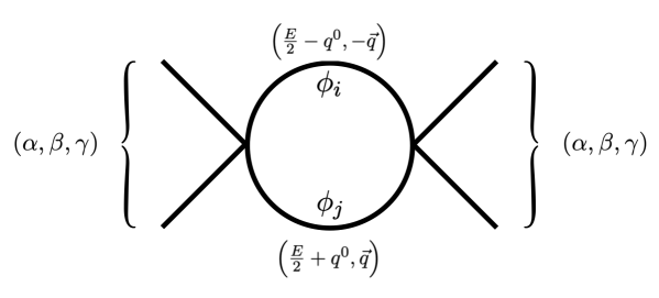
Figure 1: The 1-loop s-wave diagram. We recall the notations: $\alpha=(\phi_{1},\phi_{1})$, $\beta=(\phi_{1},\phi_{2})$, and $\gamma=(\phi_{2},\phi_{2})$. This picture includes all possible processes: (1) $\alpha\to\alpha$ through fields $\phi_{2}$ (so $\phi_{i}=\phi_{j}=\phi_{2}$ in that case and both vertices are $\lambda_{3}$); (2) $\alpha\to\alpha$ through fields $\phi_{1}$; (3) $\alpha\to\gamma$ through fields $\phi_{1}$; (4) $\alpha\to\gamma$ through fields $\phi_{2}$; (5) $\gamma\to\gamma$ through fields $\phi_{1}$; (6) $\gamma\to\gamma$ through field $\phi_{2}$; (7) $\beta\to\beta$ through fields $\phi_{1}$ and $\phi_{2}$.

Energy-momentum conservation laws are chosen as follows:

$$E_{1}+E_{2}=E=E_{3}+E_{4},$$ (49)

$$\vec{p}_{1}+\vec{p}_{2}=\vec{p}_{3}+\vec{p}_{4}=0,$$ (50)

$$\vec{p}_{1}=-\vec{p}_{2},\quad\vec{p}_{3}=-\vec{p}_{4},$$ (51)

$$|\vec{p}_{1}|=|\vec{p}_{2}|,\quad|\vec{p}_{3}|=|\vec{p}_{4}|,$$ (52)

while dispersion relations are

$$\sqrt{p_{1}^{2}u_{1}^{2}+m_{1}^{2}} =E_{1},$$ (53)

$$\sqrt{p_{2}^{2}u_{2}^{2}+m_{2}^{2}} =E_{2},$$ (54)

$$\sqrt{p_{3}^{2}u_{3}^{2}+m_{3}^{2}} =E_{3},$$ (55)

$$\sqrt{p_{4}^{2}u_{4}^{2}+m_{4}^{2}} =E_{4}.$$ (56)

First option is to consider two identical particles in the intermediate state (i.e. in the loop). There are six 1-loop diagrams of this type: (1) $\alpha\to\alpha$ through fields $\phi_{2}$; (2) $\alpha\to\alpha$ through fields $\phi_{1}$; (3) $\alpha\to\gamma$ through fields $\phi_{1}$; (4) $\alpha\to\gamma$ through fields $\phi_{2}$; (5) $\gamma\to\gamma$ through fields $\phi_{1}$; and (6) $\gamma\to\gamma$ through field $\phi_{2}$. Let us consider the process $\alpha\to\alpha$ through fields $\phi_{2}$, so the corresponding expression reads

$$iM^{(1)}_{1-\text{loop}} =\frac{1}{2}(i\lambda_{3})^{2}\int\frac{d^{4}q}{(2\pi)^{4}}\frac{i}{(\frac{l}{2}-q)^{2}-m_{2}^{2}+i\epsilon}\frac{i}{(\frac{l}{2}+q)^{2}-m_{2}^{2}+i\epsilon}$$

$$=\frac{\lambda_{3}^{2}}{2}\int\frac{d^{4}q}{(2\pi)^{4}}\frac{1}{(\frac{E}{2}-q^{0})^{2}-u_{2}^{2}\vec{q\;}^{2}-m_{2}^{2}+i\epsilon}\frac{1}{(\frac{E}{2}+q^{0})^{2}-u_{2}^{2}\vec{q\;}^{2}-m_{2}^{2}+i\epsilon},$$ (57)

where without loss of generalities we choose 4-vector as $l^{\mu}=(E,0)$. The choice of momenta is shown in Fig. 1. There are identical particles in loop, thus we write $\frac{1}{2}$ symmetry factor in the expression above. The integrand of expression for $iM^{(1)}_{\text{loop}}$ has four poles by the integration variable $q^{0}$ at the locations

$$q^{0}_{1} =\frac{E}{2}-\sqrt{u_{2}^{2}|\vec{q\;}|^{2}+m^{2}_{2}}+i\epsilon^{\prime},$$ (58)

$$q^{0}_{2} =\frac{E}{2}+\sqrt{u_{2}^{2}|\vec{q\;}|^{2}+m^{2}_{2}}-i\epsilon^{\prime},$$ (59)

coming from the first denominator in (3) and

$$q^{0}_{3} =-\frac{E}{2}+\sqrt{u_{2}^{2}|\vec{q\;}|^{2}+m^{2}_{2}}-i\epsilon^{\prime},$$ (60)

$$q^{0}_{4} =-\frac{E}{2}-\sqrt{u_{2}^{2}|\vec{q\;}|^{2}+m^{2}_{2}}+i\epsilon^{\prime},$$ (61)

from the second one. Here $\epsilon^{\prime}$ is just another redefined small parameter; $\epsilon^{\prime}>0$ and $\epsilon^{\prime}\to 0$. Two of these poles lie above the real $q^{0}$ axis and two lie below. We will close the integration contour downward and pick up the residues of the poles in the lower half-plane:

$$q^{0}_{2} =\frac{E}{2}+\sqrt{u_{2}^{2}|\vec{q\;}|^{2}+m^{2}_{2}}-i\epsilon^{\prime},$$ (62a)

$$q^{0}_{3} =-\frac{E}{2}+\sqrt{u_{2}^{2}|\vec{q\;}|^{2}+m^{2}_{2}}-i\epsilon^{\prime},$$ (62b)

Of these, only the pole at $q^{0}_{3}$ will contribute to the imaginary part of $M^{(1)}_{\text{loop}}$. We put detailed calculations of the residues in both poles in App. A. After all calculations we arrive to following contribution to the imaginary part of the corresponding matrix element:

$$\text{Im }M^{(1)}_{1-\text{loop}}=\frac{\lambda_{3}^{2}}{4}\int\frac{q^{2}dq}{2\pi}\frac{\delta(E-2\sqrt{u_{2}^{2}q^{2}+m_{2}^{2}})}{E\sqrt{u_{2}^{2}q^{2}+m_{2}^{2}}}=\frac{\lambda_{3}^{2}}{8u_{2}^{3}E}\frac{\sqrt{\Big{(}\frac{E}{2}\Big{)}^{2}-m_{2}^{2}}}{2\pi},$$ (63)

where $q\equiv|\vec{q}\;|$. Using notations $E_{(2)}\equiv\frac{E}{2}$ and $u_{2}p_{(2)}\equiv\sqrt{E_{(2)}^{2}-m_{2}^{2}}$ we obtain

$$\text{Im }M^{(1)}_{\text{loop}}=\frac{\lambda_{3}^{2}}{16\pi}\frac{p_{(2)}}{E_{(2)}}\frac{1}{2u_{2}^{2}}.$$ (64)

The subscript “$(2)$” reflects that there is the particles related to $\phi_{2}$ field “run” in the loop. Proceeding fully the same steps, one can find the answers for the rest options with identical particles in the loop. We will list all the answers later on. Now, let us consider the final option, where loop includes two different particles, i.e. (7) $\beta\to\beta$ through fields $\phi_{1}$ and $\phi_{2}$:

$$iM^{(7)}_{1-\text{loop}}=\lambda_{3}^{2}\int\frac{d^{4}q}{(2\pi)^{4}}\frac{1}{(\frac{E}{2}-q^{0})^{2}-u_{1}^{2}\vec{q\;}^{2}-m_{1}^{2}+i\epsilon_{1}}\frac{1}{(\frac{E}{2}+q^{0})^{2}-u_{2}^{2}\vec{q\;}^{2}-m_{2}^{2}+i\epsilon_{2}},$$ (65)

with poles at

$$q^{0}_{1} =\frac{E}{2}-\sqrt{u_{1}^{2}|\vec{q\;}|^{2}+m^{2}_{1}}+i\epsilon^{\prime}_{1},$$ (66a)

$$q^{0}_{2} =\frac{E}{2}+\sqrt{u_{1}^{2}|\vec{q\;}|^{2}+m^{2}_{1}}-i\epsilon^{\prime}_{1},$$ (66b)

$$q^{0}_{3} =-\frac{E}{2}+\sqrt{u_{2}^{2}|\vec{q\;}|^{2}+m^{2}_{2}}-i\epsilon^{\prime}_{2},$$ (66c)

$$q^{0}_{4} =-\frac{E}{2}-\sqrt{u_{2}^{2}|\vec{q\;}|^{2}+m^{2}_{2}}+i\epsilon^{\prime}_{2}.$$ (66d)

We choose contour in the same way as for the rest of matrix elements above and take the poles under the real axis, i.e. $q^{0}_{2}$ and $q^{0}_{3}$. The derivation of the residues in these poles are given in App. A as well. The corresponding contribution to Im $M^{(7)}_{\text{loop}}$ is

$$\text{Im}\;M^{(7)}_{1-\text{loop}}=\lambda_{3}^{2}\int\frac{q^{2}dq}{4\pi}\frac{1}{\sqrt{u_{2}^{2}\vec{q\;}^{2}+m_{2}^{2}}}\frac{\delta(E-\sqrt{u_{1}^{2}\vec{q\;}^{2}+m_{1}^{2}}-\sqrt{u_{2}^{2}\vec{q\;}^{2}+m_{2}^{2}})}{E-\sqrt{u_{2}^{2}\vec{q\;}^{2}+m_{2}^{2}}+\sqrt{u_{1}^{2}\vec{q\;}^{2}+m_{1}^{2}}},$$ (67)

what provides

$$\text{Im}\;M^{(7)}_{1-\text{loop}}=\frac{\lambda_{3}^{2}}{8\pi}\frac{p_{(1,2)}}{(u_{1}^{2}\sqrt{u_{2}^{2}p_{(1,2)}^{2}+m_{2}^{2}}+u_{2}^{2}\sqrt{u_{1}^{2}p_{(1,2)}^{2}+m_{1}^{2}})},$$ (68)

where $p_{(1,2)}$ is the root of $E-\sqrt{u_{1}^{2}p_{(1,2)}^{2}+m_{1}^{2}}-\sqrt{u_{2}^{2}p_{(1,2)}^{2}+m_{2}^{2}}=0$ equation. The subscript “$(1,2)$” means that we have two different particles (i.e. of different types) in the loop.

To sum up, we recall that

$$\text{Im}\;a_{0,\text{1-loop}}=\frac{1}{16\pi}\mbox{Im}\,M_{\text{1-loop}},$$ (69)

and collect all results in one matrix, so $\mbox{Im}\,M_{\text{1-loop}}$ equals

$$\begin{pmatrix}\frac{\lambda_{1}^{2}}{16\pi}\frac{p_{(1)}}{E_{(1)}}\frac{1}{2u_{1}^{2}}+\frac{\lambda_{3}^{2}}{16\pi}\frac{p_{(2)}}{E_{(2)}}\frac{1}{2u_{2}^{2}}&0&\frac{\lambda_{1}\lambda_{3}}{16\pi}\frac{p_{(1)}}{E_{(1)}}\frac{1}{2u_{1}^{2}}+\frac{\lambda_{2}\lambda_{3}}{16\pi}\frac{p_{(2)}}{E_{(2)}}\frac{1}{2u_{2}^{2}}\\ 0&\frac{\lambda_{3}^{2}}{8\pi}\frac{p_{(1,2)}}{(u_{1}^{2}\sqrt{u_{2}^{2}p_{(1,2)}^{2}+m_{2}^{2}}+u_{2}^{2}\sqrt{u_{1}^{2}p_{(1,2)}^{2}+m_{1}^{2}})}&0\\ \frac{\lambda_{1}\lambda_{3}}{16\pi}\frac{p_{(1)}}{E_{(1)}}\frac{1}{2u_{1}^{2}}+\frac{\lambda_{2}\lambda_{3}}{16\pi}\frac{p_{(2)}}{E_{(2)}}\frac{1}{2u_{2}^{2}}&0&\frac{\lambda_{2}^{2}}{16\pi}\frac{p_{(2)}}{E_{(2)}}\frac{1}{2u_{1}^{2}}+\frac{\lambda_{3}^{2}}{16\pi}\frac{p_{(1)}}{E_{(1)}}\frac{1}{2u_{1}^{2}}\end{pmatrix}$$ (70)

where the position of each answer is related to the same notation as in (47).

Now, write the unitarity relation (41) for the $\alpha\to\alpha$ processes:

$$\text{Im}\;a_{\alpha\alpha} =\frac{1}{2u_{\alpha}^{2}}\frac{p_{\alpha}}{E_{p_{\alpha}}}a_{\alpha\alpha}a^{*}_{\alpha\alpha}+\frac{2p_{\beta}}{(E_{2}u^{2}_{1\beta}+E_{1}u^{2}_{2\beta})}a_{\alpha\beta}a^{*}_{\beta\alpha}+\frac{1}{2u_{\gamma}^{2}}\frac{p_{\gamma}}{E_{p_{\gamma}}}a_{\alpha\gamma}a^{*}_{\gamma\alpha}.$$ (71)

As it was mentioned above, in the theory (3) it is impossible to proceed the process $\alpha\to\alpha$ through two different particles in the loop. Indeed, $a_{\alpha\beta}$ (and $a^{*}_{\beta\alpha}$) is zero, see (47), so

$$\text{Im}\;a_{\alpha\alpha} =\frac{1}{2u_{\alpha}^{2}}\frac{p_{\alpha}}{E_{p_{\alpha}}}a_{\alpha\alpha}a^{*}_{\alpha\alpha}+\frac{1}{2u_{\gamma}^{2}}\frac{p_{\gamma}}{E_{p_{\gamma}}}a_{\alpha\gamma}a^{*}_{\gamma\alpha}.$$ (72)

Using (48) as well as (64), (69), and (70), we find out that unitarity relation (41) indeed holds. One can easily check that it holds for the rest processes ($\alpha\to\gamma$, $\gamma\to\gamma$, and $\beta\to\beta$) as well.

Last but not least we present the specific bound coming from inequality (45) for the current model (3). Let us consider only $\alpha\to\alpha$ process, since the derivations for the rest are totally the same. For chosen $\alpha\to\alpha$ process we immediately arrive to the bound in the form:

$$\Big{|}\frac{\lambda_{1}}{16\pi}\frac{p_{(1)}}{2u_{1}^{2}E_{(1)}}\Big{|}\leq\frac{1}{2},\quad l=0,\quad E_{(1)}=\sqrt{u_{1}^{2}p_{(1)}^{2}+m_{1}^{2}},$$ (73)

or in terms of energy only

$$\left|\frac{\lambda_{1}}{16\pi}\frac{\sqrt{E_{(1)}^{2}-m_{1}^{2}}}{2u_{1}^{3}E_{(1)}}\right|\leq\frac{1}{2},$$ (74)

where we subsequently have used (42b), (43), and (45). The analog of (74) bound in more complicated models can give non-trivial conditions on model parameters, see, for instance, the applications to the cosmological context in Ref. Ageeva:2022asq ; Ageeva:2023nwf , and more about unitarity bounds in Ref. Pueyo:2024twm .

4 Towards a full anisotropy

In further research we are going to address the optical theorem and unitarity relation in the case of fully anisotropic dispersion relation, i.e. for theory with the following Lagrangian

$$S=\sum_{i}S_{\phi_{i}}\;,$$ (75)

$$S_{\phi_{i}}=\int d^{4}x\left(\frac{1}{2}\dot{\phi_{i}}^{2}-\frac{1}{2}u_{x,i}^{2}(\partial_{x}\phi_{i})^{2}-\frac{1}{2}u_{y,i}^{2}(\partial_{y}\phi_{i})^{2}-\frac{1}{2}u_{z,i}^{2}(\partial_{y}\phi_{i})^{2}-\frac{1}{2}m_{i}^{2}\phi_{i}^{2}\right).$$ (76)

For instance, consider the following integral (which indeed arises in such model)

$$iM_{\text{loop}} \propto\int\frac{d^{4}q}{(2\pi)^{4}}\frac{i}{(\frac{l}{2}-q)^{2}-m_{1}^{2}+i\epsilon}\frac{i}{(\frac{l}{2}+q)^{2}-m_{1}^{2}+i\epsilon}$$

$$=\int\frac{d^{4}q}{(2\pi)^{4}}\frac{i}{(\frac{E}{2}-q^{0})^{2}-u_{x,1}^{2}q_{x}^{2}-u_{y,1}^{2}q_{y}^{2}-u_{z,1}^{2}q_{z}^{2}-m_{1}^{2}+i\epsilon}$$

$$\times\frac{i}{(\frac{E}{2}+q^{0})^{2}-u_{x,1}^{2}q_{x}^{2}-u_{y,1}^{2}q_{y}^{2}-u_{z,1}^{2}q_{z}^{2}-m_{1}^{2}+i\epsilon}.$$ (77)

One can see, that integral by $q_{0}$ can be taken in the same way as integrals in the Sec. 3, so after integration by $q_{0}$ we again take only imaginary part of $M_{\text{loop}}$, which is proportional to

$$\text{Im}\;M_{\text{loop}}\propto\int\frac{d^{3}q}{(2\pi)^{4}}\frac{1}{2E\sqrt{u_{x,1}^{2}q_{x}^{2}+u_{y,1}^{2}q_{y}^{2}+u_{z,1}^{2}q_{z}^{2}+m_{2}^{2}}}$$

$$\times\Big{[}-i\pi\delta\Big{(}E-2\sqrt{u_{x,1}^{2}q_{x}^{2}+u_{y,1}^{2}q_{y}^{2}+u_{z,1}^{2}q_{z}^{2}+m_{2}^{2}}\Big{)}\Big{]}.$$ (78)

Next, performing the following change of variables: $q_{x}\to u_{x}q_{x}$, $q_{y}\to u_{y}q_{y}$, $q_{z}\to u_{z}q_{z}$, we obtain

$$\text{Im}\;M_{\text{loop}}\propto\frac{1}{u_{x}u_{y}u_{z}}\int\frac{d^{3}q}{(2\pi)^{4}}\frac{1}{2E\sqrt{q_{x}^{2}+q_{y}^{2}+q_{z}^{2}+m_{2}^{2}}}$$

$$\times\Big{[}-i\pi\delta\Big{(}E-2\sqrt{q_{x}^{2}+q_{y}^{2}+q_{z}^{2}+m_{2}^{2}}\Big{)}\Big{]}$$

$$=\frac{1}{u_{x}u_{y}u_{z}}\int\frac{4\pi q^{2}dq}{(2\pi)^{4}}\frac{1}{2E\sqrt{q^{2}+m_{2}^{2}}}\Big{[}-i\pi\delta\Big{(}E-2\sqrt{q^{2}+m_{2}^{2}}\Big{)}\Big{]},$$ (79)

what up to new factor $\frac{1}{u_{x}u_{y}u_{z}}$ coincides with the intermediate result for $M^{(1)}_{1-\text{loop}}$ from Sec. 3. This short calculation provides a naive hint about which new factors in the generalization of optical theorem (41) we could obtain.

5 Effective potential

Now turn to the calculation of one-loop potential in the background field formalism for the action given by (3).

To compute the one-loop correction, we consider small fluctuations around the background fields in (3) $\phi_{1}=\phi_{1c}+\delta\phi_{1}$ and $\phi_{2}=\phi_{2c}+\delta\phi_{2}$. For constant background fields $\phi_{1}=\phi_{1c}$ and $\phi_{2}=\phi_{2c}$, the kinetic terms vanish, and the classical potential is obtained directly from the potential terms in the Lagrangian:

$$V_{\text{classical}}(\phi_{1c},\phi_{2c})=\frac{1}{2}m_{1}^{2}\phi_{1c}^{2}+\frac{1}{2}m_{2}^{2}\phi_{2c}^{2}+\frac{\lambda_{3}}{4}\phi_{1c}^{2}\phi_{2c}^{2}+\frac{\lambda_{1}}{4!}\phi_{1c}^{4}+\frac{\lambda_{2}}{4!}\phi_{2c}^{4}.$$ (80)

Expanding the Lagrangian up to quadratic order in the fluctuations $\delta\phi_{1}$ and $\delta\phi_{2}$, as higher-order terms contribute to multi-loop corrections beyond the scope of this calculation. Substituting into the Lagrangian and retaining only the quadratic terms, we obtain:

$$\mathcal{L}_{\text{quad}}=\frac{1}{2}(\partial_{0}\delta\phi_{1})^{2}-\frac{u_{1}^{2}}{2}(\nabla\delta\phi_{1})^{2}+\frac{1}{2}(\partial_{0}\delta\phi_{2})^{2}-\frac{u_{2}^{2}}{2}(\nabla\delta\phi_{2})^{2}-$$ (81)

$$-\frac{1}{2}m_{1,\text{eff}}^{2}\delta\phi_{1}^{2}-\frac{1}{2}m_{2,\text{eff}}^{2}\delta\phi_{2}^{2}-\lambda_{3}\phi_{1c}\phi_{2c}\cdot\delta\phi_{1}\delta\phi_{2},$$ (82)

where we introduced the effective masses

$$m_{1,\text{eff}}^{2}=m_{1}^{2}+\frac{\lambda_{3}}{2}\phi_{2c}^{2}+\frac{\lambda_{1}}{2}\phi_{1c}^{2},\quad m_{2,\text{eff}}^{2}=m_{2}^{2}+\frac{\lambda_{3}}{2}\phi_{1c}^{2}+\frac{\lambda_{2}}{2}\phi_{2c}^{2}.$$ (83)

Using these, the quadratic Lagrangian becomes:

Defining the fluctuation vector $\Phi=\left(\delta\phi_{1},\delta\phi_{2},\right)$ the quadratic action acquires the form

$$S^{(2)}=\frac{1}{2}\int\frac{d^{4}k}{(2\pi)^{4}}\tilde{\Phi}(-k)^{T}\mathcal{D}(k)\tilde{\Phi}(k),$$ (84)

where fluctuation matrix $\mathcal{D}(k)$ is given by

$$\mathcal{D}(k)=\begin{pmatrix}k_{0}^{2}-u_{1}^{2}\mathbf{k}^{2}+m_{1,\text{eff}}^{2}&\lambda_{3}\phi_{1c}\phi_{2c}\\ \lambda_{3}\phi_{1c}\phi_{2c}&k_{0}^{2}-u_{2}^{2}\mathbf{k}^{2}+m_{2,\text{eff}}^{2}\end{pmatrix}$$ (85)

Here, $\mathbf{k}^{2}=k_{x}^{2}+k_{y}^{2}+k_{z}^{2}$, and the sound speeds $u_{1}^{2}$ and $u_{2}^{2}$ scale the spatial momentum terms, reflecting the modified dispersion relations.

The one-loop correction to the effective potential arises from the Gaussian integration over the fluctuations and is given by the logarithm of the functional determinant of the inverse propagator:

$$V_{\text{1-\text{loop}}}=\frac{1}{2}\int\frac{d^{4}k}{(2\pi)^{4}}\ln\det\mathcal{D}(k).$$ (86)

The determinant of the matrix $\mathcal{D}(k)$ is:

$$\det\mathcal{D}(k)=\left(k_{0}^{2}-u_{1}^{2}\mathbf{k}^{2}+m_{1,\text{eff}}^{2}\right)\left(k_{0}^{2}-u_{2}^{2}\mathbf{k}^{2}+m_{2,\text{eff}}^{2}\right)-(\lambda_{3}\phi_{1c}\phi_{2c})^{2}.$$ (87)

Defining $A(k)=k_{0}^{2}-u_{1}^{2}\mathbf{k}^{2}+m_{1,\text{eff}}^{2}$, $B(k)=k_{0}^{2}-u_{2}^{2}\mathbf{k}^{2}+m_{2,\text{eff}}^{2}$, and $C=\lambda_{3}\phi_{1c}\phi_{2c}$, the equation is: the eigenvalues of $\mathcal{D}(k)$ are given by

$$\lambda_{1,2}(k)=\frac{A(k)+B(k)\pm\sqrt{(A(k)-B(k))^{2}+4C^{2}}}{2}.$$ (88)

or

$$\lambda_{1,2}(k)=\frac{2k_{0}^{2}-(u_{1}^{2}+u_{2}^{2})\mathbf{k}^{2}+m_{+}\pm\sqrt{\left((u_{2}^{2}-u_{1}^{2})\mathbf{k}^{2}+m_{-}\right)^{2}+4(\lambda_{3}\phi_{1c}\phi_{2c})^{2}}}{2},$$

where we introduced $m_{\pm}=m_{1,\text{eff}}^{2}\pm m_{2,\text{eff}}^{2}$, $\Delta u^{2}=u_{1}^{2}-u_{2}^{2}$, and $s=\lambda_{3}\phi_{1c}\phi_{2c}$ to keep the formulas concise. Since $\ln\det\mathcal{D}(k)=\ln\lambda_{1}(k)+\ln\lambda_{2}(k)$, the one-loop correction becomes:

$$V_{\text{1-\text{loop}}}=\frac{1}{2}\int\frac{d^{4}k}{(2\pi)^{4}}\ln\lambda_{1}(k)+\frac{1}{2}\int\frac{d^{4}k}{(2\pi)^{4}}\ln\lambda_{2}(k).$$ (89)

Integrating over $k_{0}$ and using common for such calculation trick

$$\int_{-\infty}^{\infty}\frac{dk_{0}}{2\pi}\ln(k_{0}^{2}+\omega_{\pm}^{2})=\omega_{\pm},$$ (90)

we reduce the effective potential to the integrals involving dispersion relations of field fluctuations

$$V_{\text{1-\text{loop}}}=\frac{1}{2}\int\frac{d^{3}\mathbf{k}}{(2\pi)^{3}}(\omega_{+}+\omega_{-}),$$ (91)

defined by

$$\omega_{\pm}^{2}(\mathbf{k})=\frac{(u_{1}^{2}+u_{2}^{2})\mathbf{k}^{2}+m_{+}\pm\sqrt{\left((u_{1}^{2}-u_{2}^{2})\mathbf{k}^{2}+m_{-}\right)^{2}+4s^{2}}}{2}.$$ (92)

The integration in (91) with (92) cannot be performed analytically, so we make the expansion when the sound speeds difference is relatively small.

Namely, introducing the mass matrix $\mathcal{W}$

$$\mathcal{W}=\begin{pmatrix}m_{1,\text{eff}}^{2}&s\\ s&m_{2,\text{eff}}^{2}\end{pmatrix}$$ (93)

with eigenvalues $w_{\pm}=\frac{1}{2}\left(m_{+}\pm\sqrt{4s^{2}+m_{-}^{2}}\right)$, assuming that $u_{2}=c_{s}+\delta$ and $u_{1}=c_{s}$ we expanding (91) in $\delta$ to the leading order obtain that

$$\omega_{\pm}=\sqrt{c_{s}^{2}\mathbf{k}^{2}+w_{\pm}}+\delta\frac{k^{2}c_{s}\left(\sqrt{\left(w_{-}-w_{+}\right){}^{2}-4s^{2}}-w_{-}+w_{+}\right)}{2\left(w_{+}-w_{-}\right)\sqrt{w_{\pm}+k^{2}c_{s}^{2}}}+O(\delta^{2}).$$ (94)

For future purpose it is useful to introduce the shorthand notation

$$P=\sqrt{\left(w_{-}-w_{+}\right){}^{2}-4s^{2}}.$$ (95)

The first term is the renowned answer in two-field model with equal sound speeds corresponding to the canonical dispersion relation of scalar field with the “‘mass” defined by eigenvalue of mass matrix. The second term provides the first order correction due to the difference of sound speeds. For large $k$ it decreases such that UV corrections are assumed to be small, while main contribution comes from IR region (k=0). Surprisingly this occurs to be a good approximation for the effective potential integral expression, see Fig.2 where blue and red line are almost stick together.

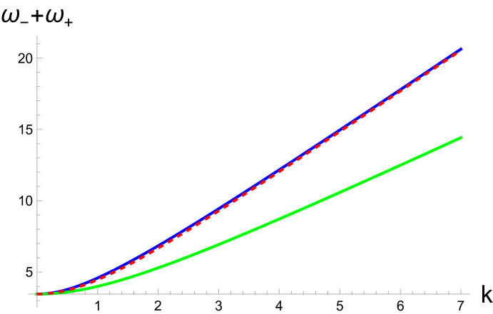
Figure 2: Blue curve corresponds to the dependence of ($\omega_{+}+\omega_{-}$) on $\mathbf{k}$ for $\delta=0.9$ and $c_{s}=1$, red dashed line corresponds to $\omega_{\pm}$ given by (94) and the green one correspond to equal unit sound speed.

To regulate the divergent integrals corresponding to $\omega_{\pm}$ expansion we use dimensional regularization and then follow $\bar{MS}$ scheme. This is the simplest option when deriving the canonical one-loop effective potential leading to the fastest route to beta functions and all necessary physical results. Different sound speeds introduce different scales, such that for our purposes the cut-off regulator as well as more delicate renormalization probably could lead us to a more refined result. However, here we would like to confine ourselves to the $\bar{MS}$ and dimensional regularization. So far $\sqrt{c_{s}^{2}\mathbf{k}^{2}+w_{\pm}}$ leading terms gives us the canonical one-loop potential $V_{1-\text{loop}}^{(0)}$ with equal sound speeds $c_{s}$

$$V_{1-\text{loop}}^{(0)}=\frac{w_{-}^{2}}{64\pi^{2}c_{s}^{3}}\left[\ln\frac{w_{-}}{\mu^{2}c_{s}^{2}}-\frac{3}{2}\right]+\frac{w_{+}^{2}}{64\pi^{2}c_{s}^{3}}\left[\ln\frac{w_{+}}{\mu^{2}c_{s}^{2}}-\frac{3}{2}\right].$$ (96)

The second order $V_{1-\text{loop}}^{(1)}$ corrections to effective potential (produced by the second term integrals in dimensional regularization in (94)) leads us to the divergent terms to be removed by counterterms

$$V_{ct,\pm}=-\frac{3\delta w_{\pm}^{2}\left(w_{-}-w_{+}+P\right)}{128\pi^{2}c_{s}^{4}\left(w_{-}-w_{+}\right)}\left(\frac{1}{\varepsilon}+\gamma_{E}-\log(4\pi)\right).$$ (97)

After the divergence subtraction the explicit form of the correction is

$$V_{1-\text{loop}}^{(1)}=\delta\frac{\left(-w_{-}+w_{+}+P\right)}{256\pi^{2}c_{s}^{4}\left(w_{-}-w_{+}\right)}\left(w_{+}^{2}\left(6\log\left(\frac{w_{+}}{c_{s}^{2}\mu^{2}}\right)-5\right)+w_{-}^{2}\left(6\log\left(\frac{w_{-}}{c_{s}^{2}\mu^{2}}\right)-5\right)\right).$$ (98)

Calculating logarithmic derivative of this correction necessary to obtain its beta functions, so one can see, that it consist of two parts

$$\mu\frac{V_{1-\text{loop}}^{(1)}}{d\mu}=\frac{3\delta}{64c_{s}^{4}\pi^{2}}\left(w_{-}^{2}+w_{+}^{2}\right)+P\cdot\frac{3\delta}{64c_{s}^{4}\pi^{2}}\left(w_{-}+w_{+}\right),$$ (99)

where the first term just gives us shifts $V_{1-\text{loop}}^{(0)}$ (and beta functions) on the value $3\delta/c_{s}^{2}$ . The second term is non-polynomial function depending on $P$ and one has to expand it in small background field values. For simplicity considering massless case one obtains that beta functions of this theory are given by

$$\beta_{\lambda_{1}}=\frac{3\left(\lambda_{3}^{2}+\lambda_{1}^{2}\right)}{16\pi^{2}c_{s}^{4}}\left(c_{s}-3/2\delta\right),$$ (100)

$$\beta_{\lambda_{2}}=\frac{3\left(\lambda_{3}^{2}+\lambda_{2}^{2}\right)}{16\pi^{2}c_{s}^{4}}\left(c_{s}-3/2\delta\right),$$ (101)

$$\beta_{\lambda_{3}}=\frac{\lambda_{3}\left(\lambda_{1}+\lambda_{2}+4\lambda_{3}\right)}{16\pi^{2}c_{s}^{4}}\left(c_{s}-3/2\delta\right).$$ (102)

So far in our approximation the original beta function scales as $c_{s}-3/2\delta$, surprisingly leading us the vanishing of beta function at spectial $\delta=2/3c_{s}$.

6 Conclusion

The study of QFTs with fields of different properties is a viable topic in the modern physics. Indeed, the applications of such theories widely appear in condensed matter physics, cosmology and many branches of high energy physics as well. In this work we consider the theory of two real massive scalar fields with different sound speeds. In this framework the generalization of optical theorem was derived, then the validity of this result was proved at the concrete model: indeed, new optical theorem holds up the the leading order by coupling constants. The generalized optical theorem now includes not only constant coefficient with sound speeds (as in Ref. Ageeva:2022byg ), but also has a dispersion relation with mass of the particle in the intermediate state. The optical theorem or unitarity relation immediately equip us with the generalized to the case of massive fields with different sound speeds unitarity bound – a powerful tool to explore the validity of any physical system. Along the unitarity bound one should also bear in mind that the consistent EFT must remain under perturbative control as one flows to higher energies. To check the latter we usually turn to the effective potential and then beta-functions evaluation since they are directly related to the renormalization-group (RG) evolution.

That is why this work also includes the derived 1-loop effective potential for the theory with massive scalar fields with different sound speeds as well as corresponding beta-functions. An interesting feature of the latter is that the beta function obtains negative contributions, revealing an unexpected fine line that appears when the sound speed difference equals the smaller sound speed multiplied by $2/3$.

As a natural extension of current results, we are going to finish the study of fully anisotropic theory (75). For instance, the latter with all different spatial components of sound speed (namely, $u_{x}$, $u_{y}$, and $u_{z}$ against the case of only one $u$ for all spatial dimensions considered in this paper) is of particular interest in the models of domain walls (see, e.g., Refs. Zeldovich:1974uw ; Dankovsky:2024zvs ; Dankovsky:2024ipq ; Babichev:2025stm ; Ai:2025bjw and references therein), since the perturbations living and propagating on this wall just can be described by the Lagrangian (75); it is supposed that the existence/taking into account the different $u_{x}$, $u_{y}$, and $u_{z}$ speeds will crucially affect the evolution of domain wall itself. Many other interesting applications of (75) can be found in different setups corresponding to anisotropic media: it can be related to condensed matter studies as in Refs. Ambegaokar ; Ticknor ; Blaschke ; Belich:2002vd ; Avila:2019xdn , or/and the studies of astrophysical magnetic fields Arth:2014jea ; Rappaz:2023rqd and many others, as well as in the theories with violated Lorentz invariance Rubtsov:2012kb ; Satunin:2017wmk : no doubt one can find other unusual applications too.

Appendix A Explicit calculations of imaginary part of one loop matrix elements from Sec. 3

This Appendix is dedicated to the evaluation of the residue in different poles for the $M^{(1)}_{1-\text{loop}}$ and $M^{(7)}_{1-\text{loop}}$ in Sec. 3. We do not write the explicit calculations for other 1-loop matrix elements since they are fully the same as for $M^{(1)}_{1-\text{loop}}$.

Residues for $M^{(1)}_{1-\text{loop}}$

We begin with the residue in pole $q^{0}_{2}$ (62a) for $M^{(1)}_{1-\text{loop}}$ given by (3). It is

$$\text{Res}\left[\frac{1}{(\frac{E}{2}-q^{0})^{2}-u_{2}^{2}\vec{q\;}^{2}-m_{2}^{2}+i\epsilon}\frac{1}{(\frac{E}{2}+q^{0})^{2}-u_{2}^{2}\vec{q\;}^{2}-m_{2}^{2}+i\epsilon}\right]_{q^{0}=q_{2}^{0}}$$

$$=\left[\frac{d}{dq_{0}}\left[\frac{1}{(\frac{E}{2}-q^{0})^{2}-u_{2}^{2}\vec{q\;}^{2}-m_{2}^{2}+i\epsilon}\right]\cdot\frac{1}{(\frac{E}{2}+q^{0})^{2}-u_{2}^{2}\vec{q\;}^{2}-m_{2}^{2}+i\epsilon}\right]_{q^{0}=q^{0}_{2}}$$

$$=\frac{1}{2\sqrt{u_{2}^{2}\vec{q\;}^{2}+m_{2}^{2}}(E^{2}+2E\sqrt{u_{2}^{2}\vec{q\;}^{2}+m_{2}^{2}}+i\epsilon^{\prime\prime})},$$ (A.1)

where $\epsilon^{\prime\prime}$ is another small parameter. Using Sokhotski$-$Plemelj theorem

$$\frac{1}{x+i\epsilon}=P\frac{1}{x}-i\pi\delta(x),$$ (A.2)

where $P$ means principle value and we arrive to

$$\frac{1}{2\sqrt{u_{2}^{2}\vec{q\;}^{2}+m_{2}^{2}}(E^{2}+2E\sqrt{u_{2}^{2}\vec{q\;}^{2}+m_{2}^{2}}+i\epsilon^{\prime\prime})}$$

$$=\frac{1}{2E\sqrt{u_{2}^{2}\vec{q\;}^{2}+m_{2}^{2}}}\left[P\frac{1}{E+2\sqrt{u_{2}^{2}\vec{q\;}^{2}+m_{2}^{2}}}-i\pi\delta(E+2\sqrt{u_{2}^{2}\vec{q\;}^{2}+m_{2}^{2}})\right],$$ (A.3)

where actually $E+2\sqrt{u_{2}^{2}\vec{q\;}^{2}+m_{2}^{2}}>0$, $E>0$ and we do not earn imaginary part from this pole since delta-function in (A) gives zero everywhere.

Consider then the second pole $q^{0}_{3}$ (62a) and residue in it reads

$$\text{Res}\left[\frac{1}{(\frac{E}{2}-q^{0})^{2}-u_{2}^{2}\vec{q\;}^{2}-m_{2}^{2}+i\epsilon}\frac{1}{(\frac{E}{2}+q^{0})^{2}-u_{2}^{2}\vec{q\;}^{2}-m_{2}^{2}+i\epsilon}\right]_{q^{0}=q_{3}^{0}}$$

$$=\left[\frac{d}{dq_{0}}\left[\frac{1}{(\frac{E}{2}+q^{0})^{2}-u_{2}^{2}\vec{q\;}^{2}-m_{2}^{2}+i\epsilon}\right]\cdot\frac{1}{(\frac{E}{2}-q^{0})^{2}-u_{2}^{2}\vec{q\;}^{2}-m_{2}^{2}+i\epsilon}\right]_{q^{0}=q^{0}_{3}}$$

$$=\frac{1}{2\sqrt{u_{2}^{2}\vec{q\;}^{2}+m_{2}^{2}}(E^{2}-2E\sqrt{u_{2}^{2}\vec{q\;}^{2}+m_{2}^{2}}+i\tilde{\epsilon}^{\prime\prime})}$$

$$=\frac{1}{2E\sqrt{u_{2}^{2}\vec{q\;}^{2}+m_{2}^{2}}}\left[P\frac{1}{E-2\sqrt{u_{2}^{2}\vec{q\;}^{2}+m_{2}^{2}}}-i\pi\delta(E-2\sqrt{u_{2}^{2}\vec{q\;}^{2}+m_{2}^{2}})\right],$$ (A.4)

and $\tilde{\epsilon}\;^{\prime\prime}\to 0$ is another small parameter. The second term in brackets in (A) equips us with the imaginary part for the $M^{(1)}_{1-\text{loop}}$. Finally, we also take into account that chosen contour is equipped with counterclockwise direction and thus we count $(-2\pi i)$ factor; after all substitutions one arrives at (63).

Residues for $M^{(7)}_{1-\text{loop}}$

Next, we consider the residues for $M^{(7)}_{1-\text{loop}}$ (65). Begin with the residue in the pole $q^{0}_{2}$ (66b); it reads

$$\text{Res}\left[\frac{1}{(\frac{E}{2}-q^{0})^{2}-u_{1}^{2}\vec{q\;}^{2}-m_{1}^{2}+i\epsilon_{1}}\frac{1}{(\frac{E}{2}+q^{0})^{2}-u_{2}^{2}\vec{q\;}^{2}-m_{2}^{2}+i\epsilon_{2}}\right]_{q^{0}=q_{2}^{0}}$$

$$=\left[\frac{d}{dq_{0}}\left[\frac{1}{(\frac{E}{2}-q^{0})^{2}-u_{1}^{2}\vec{q\;}^{2}-m_{1}^{2}+i\epsilon_{1}}\right]\cdot\frac{1}{(\frac{E}{2}+q^{0})^{2}-u_{2}^{2}\vec{q\;}^{2}-m_{2}^{2}+i\epsilon_{2}}\right]_{q^{0}=q^{0}_{2}}$$

$$=\frac{1}{(-2i\epsilon_{1}^{\prime}+2\sqrt{u_{1}^{2}\vec{q\;}^{2}+m_{1}^{2}})}$$

$$\times\frac{1}{(E+\sqrt{u_{1}^{2}\vec{q\;}^{2}+m_{1}^{2}}+\sqrt{u_{2}^{2}\vec{q\;}^{2}+m_{2}^{2}}-i\epsilon_{3})(E+\sqrt{u_{1}^{2}\vec{q\;}^{2}+m_{1}^{2}}-\sqrt{u_{2}^{2}\vec{q\;}^{2}+m_{2}^{2}}+i\epsilon_{4})},$$ (A.5)

where

$$\epsilon_{3}=\epsilon^{\prime}_{1}+\epsilon^{\prime}_{2},$$ (A.6)

$$\epsilon_{4}=\epsilon^{\prime}_{2}-\epsilon^{\prime}_{1},$$ (A.7)

where $\epsilon_{3,4}\to 0$ and $\epsilon_{3}>0$, while the sign of $\epsilon_{4}$ is undefined. The residue in the second pole $q^{0}_{3}$ (66c) is:

$$\text{Res}\left[\frac{1}{(\frac{E}{2}-q^{0})^{2}-u_{1}^{2}\vec{q\;}^{2}-m_{1}^{2}+i\epsilon_{1}}\frac{1}{(\frac{E}{2}+q^{0})^{2}-u_{2}^{2}\vec{q\;}^{2}-m_{2}^{2}+i\epsilon_{2}}\right]_{q^{0}=q_{3}^{0}}$$

$$=\left[\frac{d}{dq_{0}}\left[\frac{1}{(\frac{E}{2}+q^{0})^{2}-u_{2}^{2}\vec{q\;}^{2}-m_{2}^{2}+i\epsilon_{2}}\right]\cdot\frac{1}{(\frac{E}{2}-q^{0})^{2}-u_{1}^{2}\vec{q\;}^{2}-m_{1}^{2}+i\epsilon_{1}}\right]_{q^{0}=q^{0}_{3}}$$

$$=\frac{1}{(2i\epsilon_{2}^{\prime}-2\sqrt{u_{2}^{2}\vec{q\;}^{2}+m_{2}^{2}})}$$

$$\times\frac{1}{(E-\sqrt{u_{2}^{2}\vec{q\;}^{2}+m_{2}^{2}}+\sqrt{u_{1}^{2}\vec{q\;}^{2}+m_{1}^{2}}+i\epsilon_{4})(-E+\sqrt{u_{1}^{2}\vec{q\;}^{2}+m_{1}^{2}}+\sqrt{u_{2}^{2}\vec{q\;}^{2}+m_{2}^{2}}-i\epsilon_{3})}.$$ (A.8)

Using Sokhotski-Plemelj theorem (A.2), we extract only terms which contribute to the imaginary part of $M^{(7)}_{1-\text{loop}}$, so for the first contribution (A) we have

$$\frac{1}{(-2i\epsilon_{1}^{\prime}+2\sqrt{u_{1}^{2}\vec{q\;}^{2}+m_{1}^{2}})}$$

$$\times\frac{1}{(E+\sqrt{u_{1}^{2}\vec{q\;}^{2}+m_{1}^{2}}+\sqrt{u_{2}^{2}\vec{q\;}^{2}+m_{2}^{2}}-i\epsilon_{3})(E+\sqrt{u_{1}^{2}\vec{q\;}^{2}+m_{1}^{2}}-\sqrt{u_{2}^{2}\vec{q\;}^{2}+m_{2}^{2}}+i\epsilon_{4})}$$

$$\to\frac{1}{2\sqrt{u_{1}^{2}\vec{q\;}^{2}+m_{1}^{2}}}\frac{\Big{(}-i\pi\delta(E+\sqrt{u_{1}^{2}\vec{q\;}^{2}+m_{1}^{2}}-\sqrt{u_{2}^{2}\vec{q\;}^{2}+m_{2}^{2}})\Big{)}\text{sign}(\epsilon_{4})}{(E+\sqrt{u_{1}^{2}\vec{q\;}^{2}+m_{1}^{2}}+\sqrt{u_{2}^{2}\vec{q\;}^{2}+m_{2}^{2}})},$$ (A.9)

and imaginary terms coming from the second expression (A) read:

$$\frac{1}{(2i\epsilon_{2}^{\prime}-2\sqrt{u_{2}^{2}\vec{q\;}^{2}+m_{2}^{2}})}$$

$$\times\frac{1}{(E-\sqrt{u_{2}^{2}\vec{q\;}^{2}+m_{2}^{2}}+\sqrt{u_{1}^{2}\vec{q\;}^{2}+m_{1}^{2}}+i\epsilon_{4})(-E+\sqrt{u_{1}^{2}\vec{q\;}^{2}+m_{1}^{2}}+\sqrt{u_{2}^{2}\vec{q\;}^{2}+m_{2}^{2}}-i\epsilon_{3})}$$

$$\to\frac{-i\pi}{2\sqrt{u_{2}^{2}\vec{q\;}^{2}+m_{2}^{2}}}\left[\frac{\delta\left(E-\sqrt{u_{1}^{2}\vec{q\;}^{2}+m_{1}^{2}}-\sqrt{u_{2}^{2}\vec{q\;}^{2}+m_{2}^{2}}\right)}{E-\sqrt{u_{2}^{2}\vec{q\;}^{2}+m_{2}^{2}}+\sqrt{u_{1}^{2}\vec{q\;}^{2}+m_{1}^{2}}}\right.$$

$$\left.+\frac{\delta\left(E-\sqrt{u_{2}^{2}\vec{q\;}^{2}+m_{2}^{2}}+\sqrt{u_{1}^{2}\vec{q\;}^{2}+m_{1}^{2}}\right)\text{sign}(\epsilon_{4})}{E-\sqrt{u_{1}^{2}\vec{q\;}^{2}+m_{1}^{2}}-\sqrt{u_{2}^{2}\vec{q\;}^{2}+m_{2}^{2}}}\right].$$ (A.10)

Let us consider the following combination now:

$$-i\pi\delta\left(E+\sqrt{u_{1}^{2}\vec{q\;}^{2}+m_{1}^{2}}-\sqrt{u_{2}^{2}\vec{q\;}^{2}+m_{2}^{2}}\right)\text{sign}(\epsilon_{4})\times$$

$$\times\left[\frac{1}{2\sqrt{u_{1}^{2}\vec{q\;}^{2}+m_{1}^{2}}}\frac{1}{(E+\sqrt{u_{1}^{2}\vec{q\;}^{2}+m_{1}^{2}}+\sqrt{u_{2}^{2}\vec{q\;}^{2}+m_{2}^{2}})}\right.$$

$$\left.+\frac{1}{2\sqrt{u_{2}^{2}\vec{q\;}^{2}+m_{2}^{2}}}\frac{1}{(E-\sqrt{u_{1}^{2}\vec{q\;}^{2}+m_{1}^{2}}-\sqrt{u_{2}^{2}\vec{q\;}^{2}+m_{2}^{2}})}\right].$$ (A.11)

The latter is nothing but the terms from (A) and (A) which are proportional to $\text{sign}(\epsilon_{4})$. If one considers $\sqrt{u_{1}^{2}\vec{q\;}^{2}+m_{1}^{2}}\geq\sqrt{u_{2}^{2}\vec{q\;}^{2}+m_{2}^{2}}$ there, then the expression is zero due to the corresponding delta function. Thus, further us assume the opposite situation: $\sqrt{u_{2}^{2}\vec{q\;}^{2}+m_{2}^{2}}>\sqrt{u_{1}^{2}\vec{q\;}^{2}+m_{1}^{2}}$; after that, we find out, that expression (A) is zero. Thus, we have only one term which gives imaginary contribution to $M^{(7)}_{1-\text{loop}}$:

$$\frac{-i\pi}{2\sqrt{u_{2}^{2}\vec{q\;}^{2}+m_{2}^{2}}}\frac{\delta\left(E-\sqrt{u_{1}^{2}\vec{q\;}^{2}+m_{1}^{2}}-\sqrt{u_{2}^{2}\vec{q\;}^{2}+m_{2}^{2}}\right)}{E-\sqrt{u_{2}^{2}\vec{q\;}^{2}+m_{2}^{2}}+\sqrt{u_{1}^{2}\vec{q\;}^{2}+m_{1}^{2}}}.$$ (A.12)

Using the latter, one can taking an integral (67) with respect to $\vec{q}$ in $M^{(7)}_{1-\text{loop}}$ and finally arrive to (68).

References

- (1) B. W. Lee, C. Quigg and H. B. Thacker, Phys. Rev. Lett. 38, 883-885 (1977) doi:10.1103/PhysRevLett.38.883
- (2) B. W. Lee, C. Quigg and H. B. Thacker, Phys. Rev. D 16, 1519 (1977) doi:10.1103/PhysRevD.16.1519
- (3) M. S. Chanowitz and M. K. Gaillard, Nucl. Phys. B 261, 379-431 (1985) doi:10.1016/0550-3213(85)90580-2
- (4) T. Corbett, O. J. P. Éboli and M. C. Gonzalez-Garcia, Phys. Rev. D 91, no.3, 035014 (2015) doi:10.1103/PhysRevD.91.035014 [arXiv:1411.5026 [hep-ph]].
- (5) J. A. Oller, Prog. Part. Nucl. Phys. 110, 103728 (2020) doi:10.1016/j.ppnp.2019.103728 [arXiv:1909.00370 [hep-ph]].
- (6) Oller J A A Brief Introduction to Dispersion Relations. With modern Applications (Heidelberg: Springer Briefs in Physics, 2019).
- (7) M. Baumgart, F. Bishara, T. Brauner, J. Brod, G. Cabass, T. Cohen, N. Craig, C. de Rham, P. Draper and A. L. Fitzpatrick, et al. [arXiv:2210.03199 [hep-ph]].
- (8) A. Lacour, J. A. Oller and U. G. Meissner, Annals Phys. 326, 241-306 (2011) doi:10.1016/j.aop.2010.06.012 [arXiv:0906.2349 [nucl-th]].
- (9) D. Gülmez, U. G. Meißner and J. A. Oller, Eur. Phys. J. C 77, no.7, 460 (2017) doi:10.1140/epjc/s10052-017-5018-z [arXiv:1611.00168 [hep-ph]].
- (10) C. Cheung, P. Creminelli, A. L. Fitzpatrick, J. Kaplan and L. Senatore, JHEP 03, 014 (2008) doi:10.1088/1126-6708/2008/03/014 [arXiv:0709.0293 [hep-th]].
- (11) C. Armendariz-Picon, T. Damour and V. F. Mukhanov, Phys. Lett. B 458, 209-218 (1999) doi:10.1016/S0370-2693(99)00603-6 [arXiv:hep-th/9904075 [hep-th]].
- (12) J. Garriga and V. F. Mukhanov, Phys. Lett. B 458, 219-225 (1999) doi:10.1016/S0370-2693(99)00602-4 [arXiv:hep-th/9904176 [hep-th]].
- (13) M. Alishahiha, E. Silverstein and D. Tong, Phys. Rev. D 70, 123505 (2004) doi:10.1103/PhysRevD.70.123505 [arXiv:hep-th/0404084 [hep-th]].
- (14) T. Kobayashi, M. Yamaguchi and J. Yokoyama, Phys. Rev. Lett. 105, 231302 (2010) doi:10.1103/PhysRevLett.105.231302 [arXiv:1008.0603 [hep-th]].
- (15) T. Kobayashi, M. Yamaguchi and J. Yokoyama, Prog. Theor. Phys. 126, 511-529 (2011) doi:10.1143/PTP.126.511 [arXiv:1105.5723 [hep-th]].
- (16) P. Creminelli, A. Nicolis and E. Trincherini, JCAP 11, 021 (2010) doi:10.1088/1475-7516/2010/11/021 [arXiv:1007.0027 [hep-th]].
- (17) K. Hinterbichler, A. Joyce, J. Khoury and G. E. J. Miller, JCAP 12, 030 (2012) doi:10.1088/1475-7516/2012/12/030 [arXiv:1209.5742 [hep-th]].
- (18) D. Pirtskhalava, L. Santoni, E. Trincherini and P. Uttayarat, JHEP 12, 151 (2014) doi:10.1007/JHEP12(2014)151 [arXiv:1410.0882 [hep-th]].
- (19) S. Nishi and T. Kobayashi, JCAP 03, 057 (2015) doi:10.1088/1475-7516/2015/03/057 [arXiv:1501.02553 [hep-th]].
- (20) T. Kobayashi, M. Yamaguchi and J. Yokoyama, JCAP 07, 017 (2015) doi:10.1088/1475-7516/2015/07/017 [arXiv:1504.05710 [hep-th]].
- (21) R. Kolevatov, S. Mironov, N. Sukhov and V. Volkova, JCAP 08, 038 (2017) doi:10.1088/1475-7516/2017/08/038 [arXiv:1705.06626 [hep-th]].
- (22) T. Qiu, J. Evslin, Y. F. Cai, M. Li and X. Zhang, JCAP 10, 036 (2011) doi:10.1088/1475-7516/2011/10/036 [arXiv:1108.0593 [hep-th]].
- (23) D. A. Easson, I. Sawicki and A. Vikman, JCAP 11, 021 (2011) doi:10.1088/1475-7516/2011/11/021 [arXiv:1109.1047 [hep-th]].
- (24) Y. F. Cai, D. A. Easson and R. Brandenberger, JCAP 08, 020 (2012) doi:10.1088/1475-7516/2012/08/020 [arXiv:1206.2382 [hep-th]].
- (25) M. Osipov and V. Rubakov, JCAP 11, 031 (2013) doi:10.1088/1475-7516/2013/11/031 [arXiv:1303.1221 [hep-th]].
- (26) T. Qiu, X. Gao and E. N. Saridakis, Phys. Rev. D 88, no.4, 043525 (2013) doi:10.1103/PhysRevD.88.043525 [arXiv:1303.2372 [astro-ph.CO]].
- (27) M. Koehn, J. L. Lehners and B. A. Ovrut, Phys. Rev. D 90, no.2, 025005 (2014) doi:10.1103/PhysRevD.90.025005 [arXiv:1310.7577 [hep-th]].
- (28) T. Qiu and Y. T. Wang, JHEP 04, 130 (2015) doi:10.1007/JHEP04(2015)130 [arXiv:1501.03568 [astro-ph.CO]].
- (29) A. Ijjas and P. J. Steinhardt, Phys. Rev. Lett. 117, no.12, 121304 (2016) doi:10.1103/PhysRevLett.117.121304 [arXiv:1606.08880 [gr-qc]].
- (30) S. Mironov, V. Rubakov and V. Volkova, JCAP 10, 050 (2018) doi:10.1088/1475-7516/2018/10/050 [arXiv:1807.08361 [hep-th]].
- (31) Y. Ageeva, P. Petrov and V. Rubakov, JHEP 01, 026 (2023) doi:10.1007/JHEP01(2023)026 [arXiv:2207.04071 [hep-th]].
- (32) P. Horava, Phys. Rev. D 79, 084008 (2009) doi:10.1103/PhysRevD.79.084008 [arXiv:0901.3775 [hep-th]].
- (33) R. C. Myers and M. Pospelov, Phys. Rev. Lett. 90, 211601 (2003) doi:10.1103/PhysRevLett.90.211601 [arXiv:hep-ph/0301124 [hep-ph]].
- (34) Y. A. Ageeva and P. K. Petrov, Phys. Usp. 66, no.11, 1134-1141 (2023) doi:10.3367/UFNe.2022.11.039259 [arXiv:2206.03516 [hep-th]].
- (35) S. R. Coleman and E. J. Weinberg, Phys. Rev. D 7, 1888-1910 (1973) doi:10.1103/PhysRevD.7.1888
- (36) I. Y. Arefeva and I. V. Volovich, [arXiv:hep-th/9412155 [hep-th]].
- (37) V. Periwal, Phys. Rev. D 52, 7328-7330 (1995) doi:10.1103/PhysRevD.52.7328 [arXiv:hep-th/9508014 [hep-th]].
- (38) A. D. Martin and T. D. Spearman, Elementary Particle Theory (North-Holland Publishing Company, Amsterdam, 1970)
- (39) J. A. Oller and D. R. Entem, Annals Phys. 411, 167965 (2019) doi:10.1016/j.aop.2019.167965 [arXiv:1810.12242 [hep-ph]].
- (40) S. De Curtis, D. Dominici and J. R. Pelaez, Phys. Rev. D 67, 076010 (2003) doi:10.1103/PhysRevD.67.076010 [arXiv:hep-ph/0301059 [hep-ph]].
- (41) Y. Ageeva and P. Petrov, Phys. Rev. D 110, no.4, 4 (2024) doi:10.1103/PhysRevD.110.043527 [arXiv:2310.18402 [hep-th]].
- (42) C. D. Pueyo, H. Goodhew, C. McCulloch and E. Pajer, [arXiv:2410.23709 [hep-th]].
- (43) Y. B. Zeldovich, I. Y. Kobzarev and L. B. Okun, Zh. Eksp. Teor. Fiz. 67, 3-11 (1974) SLAC-TRANS-0165.
- (44) I. Dankovsky, E. Babichev, D. Gorbunov, S. Ramazanov and A. Vikman, JCAP 09, 047 (2024) doi:10.1088/1475-7516/2024/09/047 [arXiv:2406.17053 [astro-ph.CO]].
- (45) I. Dankovsky, S. Ramazanov, E. Babichev, D. Gorbunov and A. Vikman, JCAP 02, 064 (2025) doi:10.1088/1475-7516/2025/02/064 [arXiv:2410.21971 [hep-ph]].
- (46) E. Babichev, I. Dankovsky, D. Gorbunov, S. Ramazanov and A. Vikman, [arXiv:2504.07902 [hep-ph]].
- (47) W. Y. Ai, M. Carosi, B. Garbrecht, C. Tamarit and M. Vanvlasselaer, [arXiv:2504.13725 [hep-ph]].
- (48) Ambegaokar V, deGennes P G, Rainer D Phys. Rev. A 9 2676 (1974).
- (49) Ticknor C, Wilson R M, Bohn J L Phys. Rev. Lett. 106 065301 (2011).
- (50) Blaschke D N Journal of Physics: Condensed Matter 33 50 503005 (2021).
- (51) H. Belich, Jr., M. M. Ferreira, Jr., J. A. Helayel-Neto and M. T. D. Orlando, Phys. Rev. D 67, 125011 (2003) [erratum: Phys. Rev. D 69, 109903 (2004)] doi:10.1103/PhysRevD.67.125011 [arXiv:hep-th/0212330 [hep-th]].
- (52) R. Avila, J. R. Nascimento, A. Y. Petrov, C. M. Reyes and M. Schreck, Phys. Rev. D 101, no.5, 055011 (2020) doi:10.1103/PhysRevD.101.055011 [arXiv:1911.12221 [hep-th]].
- (53) A. Arth, K. Dolag, A. M. Beck, M. Petkova and H. Lesch, [arXiv:1412.6533 [astro-ph.CO]].
- (54) Y. Rappaz and J. Schober, Astron. Astrophys. 683, A35 (2024) doi:10.1051/0004-6361/202347497 [arXiv:2307.09451 [astro-ph.CO]].
- (55) G. Rubtsov, P. Satunin and S. Sibiryakov, Phys. Rev. D 86, 085012 (2012) doi:10.1103/PhysRevD.86.085012 [arXiv:1204.5782 [hep-ph]].
- (56) P. Satunin, Phys. Rev. D 97, no.12, 125016 (2018) doi:10.1103/PhysRevD.97.125016 [arXiv:1705.07796 [hep-th]].