Emerging (2+1)D electrodynamics and topological instanton in pseudo-Hermitian two-level systems

Abstract

We reveal a hidden electrodynamical structure emerging from a general $2\times 2$ pseudo-Hermitian system that exhibits real spectra. Even when the Hamiltonian does not explicitly depend on time, the Berry curvature can be mapped onto a $2+1$ dimensional electromagnetic field arising from an artificial spacetime instanton, in sharp contrast to the Hermitian systems where the Berry curvature is equivalent to the static magnetic field of a magnetic monopole in three spatial dimensions. The instanton appearing as a spacetime singularity carries a topological charge that quantizes the jump of magnetic flux of the Berry curvature at the time origin. Our findings are demonstrated in a simple example related to antiferromagnetic magnons.

Geometric (Berry) phases and their topological origins entail profound implications in the physical behavior of quantum systems [1, 2, 3, 4, 5]. In a general Hermitian quantum system, if the Hamiltonian depends on time implicitly through an adiabatic parameter $\bm{R}(t)$ but is not explicitly time-dependent, namely $H=H[\bm{R}(t)]$ rather than $H(\bm{R},t)$, the Berry phase is purely geometrical and can be viewed as the flux of a static magnetic field (Berry curvature) residing in the parameter space spanned by $\bm{R}$, so long as $|d\bm{R}/dt|$ is much smaller than the energy gap—known as the adiabatic condition [1]. Unlike real magnetic fields that are always divergenless, the Berry curvature diverges at the energy degenerate points which play the role of artificial magnetic monopoles [6, 7]. The monopoles carry quantized magnetic charges that characterize the topological properties of the system.

However, for open and dissipative quantum systems that are typically described by non-Hermitian Hamiltonians, complex energy eigenvalues may arise, rendering the system unstable—either growing or decaying in time. The associated Berry phases could also become complex valued, compromising its geometrical interpretation. A salient exception is the pseudo-Hermitian (PH) systems, whose Hamiltonian satisfy

$$H^{\dagger}(\bm{R})=\eta\,H(\bm{R})\,\eta^{-1},$$ (1)

where $\eta$ is invertible, Hermitian, and independent of $\bm{R}$ . Under such constraint, the eigenvalues of $H$ are either strictly real or appearing in complex-conjugate pairs [9, 10, 11, 12]. Prior studies suggested that a real spectrum is crucial for defining a meaningful Berry phase [13, 14, 15]. Meanwhile, so long as real spectra are guaranteed, all non-Hermitian systems fall into the same class as PH systems [9, 10, 11]. Therefore, by focusing on the PH systems, one can effectively encompass all non-Hermitian models with real eigenvalues. Within the biorthonormal framework [16, 17], a well-behaved and real Berry phase can be justified by the PH condition [See the Supplemental Material (SM)]. Nevertheless, what remains elusive is a magnetic interpretation, hence an intuitive analogy, of the Berry phases and their corresponding singularities serving as topological invariants.

In this Letter, we explore a generic $2\times 2$ PH Hamiltonian exhibiting real spectra, which supports a unique Berry curvature that resembles a $2+1$ dimensional (D) electromagnetic field but cannot be simply mapped onto a static magnetic field as its Hermitian counterpart, despite that the Hamiltonian $H(\bm{R})$ does not explicitly depend on time. The pivotal factor lies in an emergent spacetime metric in the parameter space such that one component of $\bm{R}$ naturally plays the role of time while the rest act as space. We find that the electric and magnetic components of the Berry curvature are inherently connected by the $(2+1)$D Faraday equation in the presence of spacetime singularities, dubbed instantons, tying to the anti-crossing points of the energy levels. The artificial instantons emerging in (real-spectral) PH systems parallel the role of magnetic monopoles appearing in Hermitian systems. This perspective unifies non-Hermitian Berry-phase physics with field-theoretic concepts, providing a novel handle on topology in open and dissipative quantum systems.

Emerging (2+1)D electrodynamics.—Let us consider a most general two-level PH system, whose Hamiltonian depends on six real parameters [11]

$$H=a_{0}\sigma_{0}+(a_{1}\bm{n}_{1}+ia_{2}\bm{n}_{2}+ia_{3}\bm{n}_{3})\cdot\bm{\sigma},$$ (2)

where $\bm{\sigma}=(\sigma_{x},\sigma_{y},\sigma_{z})$ are the Pauli matrices, $\sigma_{0}$ is the identity matrix, while $\bm{n}_{1}=(\sin{\theta}\cos{\phi},\sin{\theta}\sin{\phi},\cos{\theta})$, $\bm{n}_{2}=(\cos{\theta}\cos{\phi},\cos{\theta}\sin{\phi},-\sin{\theta})$, and $\bm{n}_{3}=\bm{n}_{1}\times\bm{n}_{2}$ form an orthonormal frame specified by $\theta$ and $\phi$. It is straightforward to solve the eigen-energies of $H$ as

$$\varepsilon_{\pm}=a_{0}\pm\sqrt{a_{1}^{2}-a_{2}^{2}-a_{3}^{2}}=a_{0}\pm\absolutevalue{\ell},$$ (3)

which are independent of $\theta$ and $\phi$ thanks to the $SO(3)$ symmetry among the base vectors $\bm{n}_{i}$ ($i=1,2,3$). The exceptional points are located on the hypersurfaces of $a_{1}^{2}=a_{2}^{2}+a_{3}^{2}$, separating stable from unstable regions of the PH system. We will focus on the real-spectral cases satisfying $a_{1}^{2}>a_{2}^{2}+a_{3}^{2}$. In this region, the biorthonormal eigenstates [16, 17] can be solved as

$$\ket{\psi^{R}_{-}} =\frac{1}{2\ell}\begin{bmatrix}-e^{i\phi}(a_{1}\sin\theta+ia_{2}\cos\theta+a_{3})\\ 1+a_{1}\cos\theta-ia_{2}\sin\theta\end{bmatrix},$$ (4a)

$$\ket{\psi^{R}_{+}} =\frac{1}{2\ell}\begin{bmatrix}e^{-i\phi}(a_{1}\sin\theta+ia_{2}\cos\theta+a_{3})\\ 1-a_{1}\cos\theta+ia_{2}\sin\theta\end{bmatrix},$$ (4b)

$$\ket{\psi^{L}_{-}} =\frac{1}{\ell}\left[\frac{e^{-i\phi}(-a_{1}\sin\theta+ia_{2}\cos\theta+a_{3})}{1+a_{1}\cos\theta+ia_{2}\sin\theta},\ 1\right]^{T},$$ (4c)

$$\ket{\psi^{L}_{+}} =\frac{1}{\ell}\left[\frac{e^{-i\phi}(-a_{1}\sin\theta+ia_{2}\cos\theta+a_{3})}{-1+a_{1}\cos\theta+ia_{2}\sin\theta},\ 1\right]^{T},$$ (4d)

where $R\,(L)$ represents the right (left) eigenstates and $\pm$ correspond to the $\pm$ energy level in Eq. (3). Here we have assumed $\ell>0$, but none of the subsequent results will be altered if $\ell<0$.

Because $a_{0}$ represents an overall energy reference in Eq. (3), which can be shifted to $0$, the parameter space is effectively 3D, spanned by $(a_{1},a_{2},a_{3})$. Then a surface of constant energy $\varepsilon_{0}=\ell$ satisfies $\ell^{2}=a_{1}^{2}-a_{2}^{2}-a_{3}^{2}$, resembling a $(2+1)$D spacetime interval in special relativity (with the speed of light $c=1$). Based on this analogy, it is tempting to identify a coordinate mapping:

$$a_{1}\rightarrow t,\quad a_{2}\rightarrow x,\quad a_{3}\rightarrow y,$$ (5)

by which we could interpret the parameter space as an artificial spacetime endowed with a Minkowski metric $\eta_{\mu\nu}=\text{diag}(1,-1,-1)$ so that $\ell^{2}=t^{2}-x^{2}-y^{2}$. Let $r^{\mu}$ enumerating through $(t,x,y)$, then $\ell^{2}=\eta_{\mu\nu}r^{\mu}r^{\nu}$. This intriguing structure implies that a $2\times 2$ PH Hamiltonian is intimately related to an emergent spacetime covariance, which can be attributed to the $SO(3)$ symmetry of the basis $\bm{n}_{i}$ under the PH condition in Eq. (1).

Using the biorthonormal eigenstates, we can define the Berry connection as ($\hbar=1$ in natural units)

$$A_{\mu}^{\pm}=i\bra{\psi^{L}_{\pm}}\partial_{\mu}\ket{\psi^{R}_{\pm}}$$ (6)

with $\partial_{\mu}\equiv\partial/\partial r^{\mu}$. Accordingly, we can define the Berry curvature as

$$F_{\mu\nu}^{\pm}=\partial_{\mu}A_{\nu}^{\pm}-\partial_{\nu}A_{\mu}^{\pm},$$ (7)

which is antisymmetric $F_{\mu\nu}^{\pm}=-F_{\nu\mu}^{\pm}$. Since $F_{\mu\nu}^{+}=-F_{\mu\nu}^{-}$ (i.e., the curvatures associated with the two energy levels always cancel), we can simplify the notations by focusing on $F_{\mu\nu}^{-}$ and omitting the $\pm$ index, unless it is necessary to specify the energy level. In the matrix form, the Berry curvature is expressed as

$$F_{\mu\nu}=\frac{-\epsilon_{\mu\nu\rho}r^{\rho}}{2\ell^{3}}=\frac{1}{2(t^{2}-x^{2}-y^{2})^{3/2}}\begin{pmatrix}0&-y&x\\ y&0&-t\\ -x&t&0\end{pmatrix},$$ (8)

where $\ell=(\eta_{\mu\nu}r^{\mu}r^{\nu})^{1/2}=\sqrt{t^{2}-x^{2}-y^{2}}$ and $\epsilon_{\mu\nu\rho}$ is the Levi-Civita symbol. The gauge field is $U(1)$ invariant because $\varepsilon_{\pm}$ is non-degenerate for $\ell\neq 0$. In terms of the electromagnetic field variables, Eq. (8) translates into

$$B=\frac{t}{2\ell^{3}},\quad E_{x}= -\frac{y}{2\ell^{3}},\quad E_{y}=\frac{x}{2\ell^{3}},$$ (9)

which is illustrated in Fig. 1(a). By sharp contrast, in an Hermitian setting, all coordinates of the parameter space are akin to pure spatial variables so that the Berry curvature can only be mapped onto a static magnetic field rather than an electromagnetic tensor.

Spacetime instanton.—The Bianchi identity requires that $\epsilon^{\rho\mu\nu}\partial_{\rho}F_{\mu\nu}=0$, corresponding to Faraday’s equation $\partial_{t}B+\hat{\bm{z}}\cdot(\bm{\nabla}_{\perp}\!\times\bm{E})=0$ where $\bm{E}=(E_{x},E_{y},0)$ and $\bm{\nabla}_{\perp}=(\partial_{x},\partial_{y},0)$ is the planar nabla operator. A naïve substitution of Eq. (9) indeed satisfies the above relation, but there is a caveat. Recall that a point charge represented by $\delta(r)$ generates an electric field proportional to $1/r^{2}$, which, upon direct application of the Gauss-Coulomb law, yields zero and cannot reproduce $\delta(r)$ [18]. This is because the spatial derivatives become ill-defined at $r\rightarrow 0$ while $\delta(r)$ is non-analytical. By the same token, properly treating the diverging behavior of Eq. (9) for $\ell\rightarrow 0$ leads to a modified equation:

$$\partial_{t}B+\hat{\bm{z}}\cdot(\bm{\nabla}_{\perp}\!\times\bm{E})=-2\pi Q\delta(t)\delta(x)\delta(y),$$ (10)

where $Q=1$ is the topological charge of an instanton located at the spacetime origin [19, 20], at which the energies becomes degenerate. It is easy to see that $Q=\mp 1$ for the $\varepsilon_{\pm}$ level, respectively.

To better appreciate the appearance of instanton as the source of Berry curvature, we turn to the dual field $\tilde{F}^{\mu}=\epsilon^{\mu\alpha\beta}F_{\alpha\beta}$, in terms of which the Bianchi identity becomes $\partial_{\mu}\tilde{F}^{\mu}=0$ away from the spacetime origin. If we regard $\tilde{F}^{\mu}$ as a 3D vector $\tilde{\bm{F}}=(-B,-E_{y},E_{x})$ and define the 3D nabla operator $\tilde{\bm{\nabla}}=(\partial_{t},\partial_{x},\partial_{y})$, then the Bianchi identity is further transformed into $\tilde{\bm{\nabla}}\cdot\tilde{\bm{F}}=0$, which enables us to intuitively reinterpret Eq. (10) as Gauss’s law in 3D:

$$\tilde{\bm{\nabla}}\cdot\tilde{\bm{F}}=2\pi Q\delta^{3}(\tilde{\bm{r}}),$$ (11)

where $\tilde{\bm{r}}=(t,x,y)$ is identified as $r^{\mu}$.

It is worthwhile emphasizing that magnetic monopoles are conceptually incompatible with the framework of $(2+1)$D Maxwell’s theory in which the magnetic field $B$ is a pseudo-scalar so that the magnetic Gauss’s law is meaningless; magnetic monopoles must yield to instantons. Nevertheless, the Faraday equation in the presence of a spacetime instanton can be intuitively placed in a hypothetical $(3+1)$D context through dimensional reduction. Specifically, if magnetic current density $\bm{J}_{m}$ exists, the $(3+1)$D Faraday’s equation reads $\bm{\nabla}\times\bm{E}+\partial_{t}\bm{B}=-\bm{J}_{m}$. When everything becomes uniform in the $z$ direction, and $\bm{J}_{m}=2\pi Q\delta(t)\delta(x)\delta(y)\hat{\bm{z}}$ represents an infinitely narrow pulse magnetic current at $t=0$, Eq.(10) is retrieved. In this regard, the instanton charge $Q$ is nothing but the amplitude of the pulse stimulus.

To further demystify the topological implication of the spacetime instanton, we consider a Gauss surface enclosing the instanton as illustrated in Fig. 1(b), which consists of two reversely oriented cones slightly detached from the lightcone by $\epsilon$ . After some tricky algebra detailed in the SM, we can associate the total flux of the dual field $\tilde{\bm{F}}$ with the topological charge $Q$ by virtue of the integral form of Eq. (11): $\oiint\tilde{\bm{F}}\cdot d\bm{s}=2\pi Q$. This relation differs from the ordinary Gauss theorem in 3D Euclidean space by a factor of $2$. In terms of the original field variables, the Gauss relation becomes

$$\Phi(t_{0})-\Phi(-t_{0})+\int_{-t_{0}}^{t_{0}}dt\oint_{C(t)}\bm{E}\cdot d\bm{l}=-2\pi Q,$$ (12)

where $\pm t_{0}$ parameterize the top and bottom lids of the Gauss surface and $\Phi(t)=\iint\bm{B}(t)\cdot d\bm{s}$ is the magnetic flux through the surface bounded by circle $C(t)$ at time $t$ (for $-t_{0}\leq t\leq t_{0}$). In the $t_{0}\rightarrow 0^{+}$ limit, $\Phi(t_{0})-\Phi(-t_{0})$ becomes $\Phi(0^{+})-\Phi(0^{-})$, i.e., the jump of magnetic flux $\Delta\Phi(0)$ at $t=0$, while $\oint_{C(0)}\bm{E}\cdot d\bm{l}$ (the vorticity of the $\bm{E}$ field) is continuous across $t=0$ so that the third term in Eq. (12) vanishes for $t_{0}\rightarrow 0^{+}$, whereas $-2\pi Q$ on the right-hand side is not affected because the instanton is still enclosed by the Gauss surface. Therefore, Eq. (12) indicates $\Delta\Phi(0)/2\pi=-Q$, entailing a neat topological interpretation: the discontinuity of magnetic flux at $t=0$ is quantized in integer multiples of $2\pi$, with the integer being the instanton number.

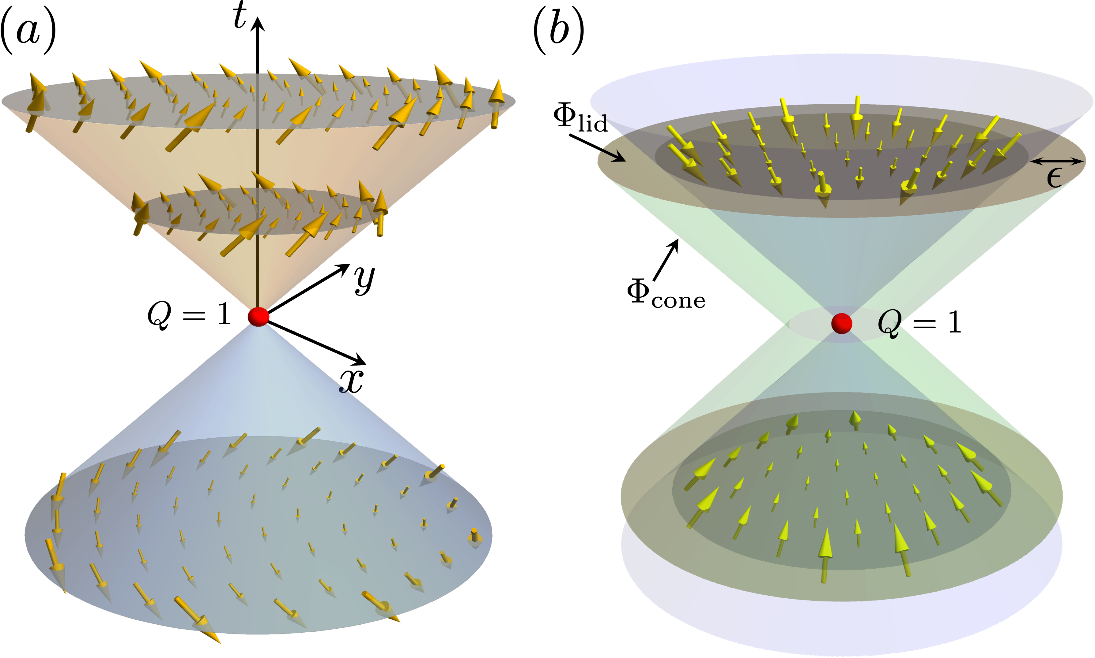
Figure 1: (a) Vector plot of the emerging gauge fields $(B,E_{x},E_{y})$ with its norm scaled logarithmically, on three parallel cutting planes within the light cone. The instanton ($Q=1$ for $\varepsilon_{-}$) is indicated by a red dot. (b) Gauss’ surface enclosing the instanton, with the dual field vector $\tilde{\bm{F}}$ plotted on two cutting planes for positive and negative $t$.

In a material context, the artificial spacetime variables $(t,x,y)$ are typically functions of the 3D crystal momentum $\bm{k}$, and the spacetime instanton corresponds to the solution of $t(\bm{k})=x(\bm{k})=y(\bm{k})=0$. In comparison, a well-known material context for the $3$D magnetic monopoles associated with Hermitian systems is the $3$D Weyl semimetals [6]. Analogous to the stability of the Weyl points, here the three equations $r^{\mu}(\bm{k})=0$ define three distinct $2$D surfaces in the $\bm{k}$ space, and their intersection (if exists) typically reduces to a point being robust against small deformations of $r^{\mu}(\bm{k})$, thus rendering the instanton topologically stable. In a PH lattice model, the total number of instantons is a topological invariant of the parameter space, obtained by integrating over the region enclosed by the Fermi surface, provided that the eigen-energies remain real. In particular, if $(k_{x},k_{y},k_{z})$ can be linearly mapped onto $(t,x,y)$ (e.g., by Taylor expansion around a high symmetry point), then the gauge-field interpretation conceived above will be directly applicable to the $\bm{k}$ space.

Field dynamics.—Concerning the emerging $(2+1)$D electrodynamics, it is instructive to check the self-dynamics of the gauge field consisting of Coulomb’s law and Ampere’s law. In this regard, we find that Eq. (8) satisfies $J_{\nu}=\partial^{\mu}F_{\mu\nu}=0$, or

$$\bm{\nabla}_{\perp}\!\cdot\bm{E}=0,\qquad\partial_{t}\bm{E}-\bm{\nabla}_{\perp}\!\times(B\hat{\bm{z}})=0,$$ (13)

meaning that both the electric charge density $J_{0}$ and the electric current density $J_{i}$ vanish exactly. Equations (10) and (13) together indicate that the Berry curvature emerging in our $2\times 2$ PH system can be described by an effective Maxwell Lagrangian density $\mathcal{L}=-F_{\mu\nu}F^{\mu\nu}$ devoid of electric sources, while the functional derivative $\delta\mathcal{L}/\delta A_{\mu}=0$ is subject to the topological constraint in the form of a spacetime instanton.

With a full set of Maxwell’s equations, our Berry curvature admits a compelling interpretation through the lens of $(2+1)$D electrodynamics. At $r^{\mu}=(0,0,0)$, an instanton flashes infinitely fast, triggering an electromagnetic wave propagating in spacetime. This scenario contrasts sharply with what one normally expects for an Hermitian system, where a static magnetic monopole persists indefinitely and never acquire any dynamics. Moreover, even when an Hermitian Hamiltonian explicitly depends on time, $H=H[\bm{R}(t),t]$ (but $\partial_{t}H$ is small enough to maintain adiabaticity), which affords both electric and magnetic components in the Berry curvature, only Faraday’s law can be satisfied whereas Coulomb’s law and Ampere’s law are baseless [22]. In other words, the gauge field emerging in an Hermitian system does not acquire self-dynamics; it can only passively affect the motion of charges but cannot be excited by the charges.

Quantum geometric tensor.—In Hermitian systems, the Berry curvature can be viewed as the anti-symmetric component of a broader geometric concept known as the quantum geometric tensor (QGT) [23], whose symmetric component is the quantum metric. Recently, the QGT has been generalized into non-Hermitian systems [24, 25, 26, 27], but little is known about its manifestation in PH systems that host topological instantons. Basing on Eq. (1), we can derive the QGT associated with a particular energy level $n$ for a general PH Hamiltonian as

$$Q_{n,\mu\nu}= \bra{\partial_{\mu}\psi_{n}^{L}}(1-P)\ket{\partial_{\nu}\psi_{n}^{R}},$$ (14)

where $P=\ket{\psi_{n}^{R}}\bra{\psi_{n}^{L}}$ is the projection operator. By exploiting the biorthonormal Hellmann–Feynman relations, we can express the QGT in terms of the eigenstates and the Hamiltonian:

$$Q_{n,\mu\nu}= \sum_{m\neq n}\frac{\bra{\psi_{n}^{L}}\partial_{\mu}H\ket{\psi_{m}^{R}}\bra{\psi_{m}^{L}}\partial_{\nu}H\ket{\psi_{n}^{R}}}{(E_{n}-E_{m})^{2}},$$ (15)

which looks similar to its Hermitian counterpart but the left and right eigenvectors are distinguishable. We find that away from the energy degenerate points, the QGT can be decomposed as

$$Q_{n,\mu\nu}= g_{n,\mu\nu}-\frac{i}{2}F_{n,\mu\nu},$$ (16)

where $g_{\mu\nu}$ is the quantum metric (a symmetric tensor) and the $F_{\mu\nu}$ is the Berry curvature we defined previously. This relation is identical to its Hermitian counterpart [4]. By inserting Eq. (4) into Eq. (15) and taking its symmetric component, we finally obtain the quantum metric associated with the spacetime instanton (with $Q=1$) in a general $2\times 2$ PH system:

$$g_{\mu\nu}=\frac{1}{4\ell^{4}}\left[\ell^{2}\eta_{\mu\nu}-(\eta_{\mu\alpha}r^{\alpha})\otimes(\eta_{\nu\beta}r^{\beta})\right]$$

$$=\frac{-1}{4(t^{2}-x^{2}-y^{2})^{2}}\begin{pmatrix}x^{2}+y^{2}&-tx&-ty\\[4.30554pt] -tx&t^{2}-y^{2}&xy\\[4.30554pt] -ty&xy&t^{2}-x^{2}\end{pmatrix},$$ (17)

which is related to the Berry curvature by

$$\frac{1}{4}F_{\mu\nu}F_{\alpha\beta}=g_{\mu\alpha}g_{\nu\beta}-g_{\mu\beta}g_{\nu\alpha}.$$ (18)

Example.—Let us consider a concrete $2\times 2$ PH Hamiltonian that can effectively describe topological magnons in transition-metal trichalcogenides with collinear antiferromagnetic order on a honeycomb lattice [28, 29]. In this setting, magnons of opposite spin species form a two-level system governed by a Schrödinger-like equation $i\hbar\sigma_{z}\partial_{\tau}\Psi=H_{0}\Psi$, where $H_{0}=tI+x\sigma_{x}+y\sigma_{y}+a_{0}\sigma_{z}$ with $\sigma_{i}$ being the Pauli matrices. The appearance of $\sigma_{z}$ on the left hand side is attributed to the bosonic Bogoliubov transformation. Multiplication of $\sigma_{z}$ on both sides yields a true PH system satisfying

$$i\hbar\partial_{\tau}\Psi=H_{\rm ph}\Psi,$$ (19)

where the Hamiltonian

$$H_{\rm ph}=\sigma_{z}H_{0}=t\sigma_{z}+ix\sigma_{y}-iy\sigma_{x}+a_{0}I$$ (20)

is a particular case of Eq. (2) for $\theta=0$, $\phi=\pi/2$, $\bm{n}_{1}=\hat{\bm{z}}$, $\bm{n}_{2}=\hat{\bm{y}}$ and $\bm{n}_{3}=-\hat{\bm{x}}$. Basing on the form of Eq. (3), we can adopt a hyperbolic parameterization

$$t=\ell\cosh{\xi},\quad x=\ell\sinh{\xi}\cos{\lambda},\quad y=\ell\sinh{\xi}\sin{\lambda},$$ (21)

which reduces the eigenstates in Eq. (4) into

$$\ket{\psi^{R}_{-}}= \begin{pmatrix}-e^{-i\lambda}\sinh{\frac{\xi}{2}}\\ \cosh{\frac{\xi}{2}}\end{pmatrix},\,\ket{\psi^{R}_{+}}=\begin{pmatrix}e^{-i\lambda}\cosh{\frac{\xi}{2}}\\ -\sinh{\frac{\xi}{2}}\end{pmatrix},$$

$$\ket{\psi^{L}_{-}}= \begin{pmatrix}e^{-i\lambda}\sinh{\frac{\xi}{2}}\\ \cosh{\frac{\xi}{2}}\end{pmatrix},\quad\ket{\psi^{L}_{+}}=\begin{pmatrix}e^{-i\lambda}\cosh{\frac{\xi}{2}}\\ \sinh{\frac{\xi}{2}}\end{pmatrix},$$ (22)

where they are all independent of $\ell$. Following a straightforward algebra elaborated in the SM, we can obtain the QGT under the $(t,\,x,\,y)$-basis and fully recover the emerging electromagnetic field in Eq. (8) featuring an instanton solution at the origin.

What is interesting here is that the QGT under the $(\ell,\,\xi,\,\lambda)$-basis becomes block diagonal with a rank equal to $2$, as all elements involving $\ell$ vanish (see details in the SM). This means that the effective dimension of the parameter space is reduced to $2$. The Berry curvature and the quantum metric residing in the $2$D space spanned by $\xi$ and $\lambda$ (for the lower band $\varepsilon_{-}$) become:

$$F_{ij} =\frac{1}{2}\begin{pmatrix}0&-\sinh{\xi}\\ \sinh{\xi}&0\end{pmatrix},$$ (23)

$$g_{ij} =\frac{-1}{4}\begin{pmatrix}1&0\\ 0&\sinh^{2}{\xi}\end{pmatrix},$$ (24)

which characterize the Hilbert space geometry on an equal energy surface (labeled by a non-zero constant $\ell$). For the upper band, $F_{ij}$ flips sign while $g_{ij}$ remains the same. In this $2$D parameter space, the Berry curvature has only one component, namely the off-diagonal element $f=(1/2)\sinh\xi$, satisfying

$$f=2\sqrt{\text{det}[g]},$$ (25)

which coincides with a well-known identify in $2\times 2$ Hermitian systems [30].

Final remarks.—It is instrumental to mention that the $2\times 2$ $\mathcal{PT}$-symmetric systems form a subclass of the general PH systems we have considered. For instance, a $\mathcal{PT}$-symmetric Hamiltonian $H_{\rm pt}=a_{0}I+ix_{0}\sigma_{x}+y_{0}\sigma_{y}+z_{0}\sigma_{z}$ satisfying $\sigma_{z}H^{*}_{\rm pt}\sigma_{z}^{-1}=H_{\rm pt}$ supports real eigenvalues

$$\varepsilon_{\pm}=a_{0}\pm\sqrt{-x_{0}^{2}+y_{0}^{2}+z_{0}^{2}},$$ (26)

which can be mapped onto Eq. (3) by identifying $x_{0}\rightarrow-a_{3}$, $y_{0}\rightarrow a_{1}\sin\theta$, and $z_{0}\rightarrow a_{1}\cos\theta$, while $a_{2}=0$ and $\theta$ is arbitrary. Under such re-parameterization, when setting $\phi=\pi/2$, Eq. (2) directly constructs our chosen $H_{\rm pt}$. Therefore, a $\mathcal{PT}$-symmetric system with purely real spectra is fully encompassed by our model.

One may wonder if there exists a mapping from a PH Hamiltonian to the $(3+1)$D electrodynamics with a full set of Maxwell equations. While Eq. (2) represents the most general $2\times 2$ PH models, its spectrum depends on only three independent variables (apart from $a_{0}$—an overall energy shift), which is insufficient to account for the six components of the $(3+1)$D electromagnetic field tensor. On the other hand, a $3\times 3$ PH Hamiltonian necessarily involves the eight Gell-Mann matrices and the identity, holding more degrees of freedom than what are needed to describe the $(3+1)$D electrodynamics. This discrepancy poses an open question for future explorations.