Relative Overfitting and Accept-Reject Framework

Abstract

Currently, the scaling law of Large Language Models (LLMs) faces challenges and bottlenecks. This paper posits that noise effects, stemming from changes in the signal-to-noise ratio under diminishing marginal returns, are the root cause of these issues. To control this noise, we investigated the differences between models with performance advantages and disadvantages, introducing the concept of "relative overfitting." Based on their complementary strengths, we have proposed an application framework, Accept-Reject (AR), and the associated AR Law, which operates within this framework to elucidate the patterns of performance changes after model integration. In Natural Language Processing (NLP), we use LLMs and Small Language Models (SLMs) as the medium for discussion. This framework enables SLMs to exert a universal positive influence on LLM decision outputs, rather than the intuitively expected potential negative influence. We validated our approach using self-built models based on mainstream architectures and pre-trained mainstream models across multiple datasets, including basic language modeling, long-context tasks, subject examination, and question-answering (QA) benchmarks. The results demonstrate that through our framework, compared to increasing the LLM’s parameters, we can achieve better performance improvements with significantly lower parameter and computational costs in many scenarios. These improvements are universal, stable, and effective. Furthermore, we explore the potential of "relative overfitting" and the AR framework in other machine learning domains, such as computer vision (CV) and AI for science. We hope the proposed approach can help scale laws overcome existing bottlenecks.

1 Introduction

Recently, the role of artificial intelligence in societal development has garnered increasing attention, particularly as the application of large language models (LLMs) significantly enhances human productivity. For an extended period, scaling laws 1 ; 2 ; 3 , driven by more data, greater computational power, and larger models, served as the guiding principle for training LLMs, allowing performance improvements through resource accumulation.

However, with the rapid advancement of artificial intelligence, scaling laws face increasing scrutiny 4 ; 5 , raising questions about whether they have reached a bottleneck. From the perspective of diminishing marginal returns, this observation is logical. While the debate continues over whether scaling laws have definitively hit a ceiling, evidence shows that the rate of performance improvement has notably decelerated. Furthermore, recent LLMs employing distillation techniques 6 ; 7 ; 8 ; 9 - where larger ’teacher’ models train smaller ’student’ models - demonstrate that SLMs can achieve performance comparable to LLMs (e.g., Deepseek R1 10 , Qwen 11 ). The DeepSeek R1 report highlights that these distillation-based models with significantly fewer parameters perform remarkably close to their larger counterparts.

In this work, we explore an approach from the perspective of signal-to-noise ratio in model data, aiming to break the scaling law bottleneck. Data serves as the cornerstone for language models, yet along with its information, it inevitably introduces noise. Furthermore, the impact of the same data differs between a simple model exposed to limited data and a complex model utilizing vast amounts of data. Based on this premise, this paper introduces the concept of "relative overfitting" to better use the information and noise within a model. It posits that models with different structures exhibit fine-grained differences when modeling the target distribution. Within the same architecture, a model that better models the target distribution demonstrates relative overfitting compared to another model. Based on exploring this concept, we propose a universally applicable method.

Specifically, this paper proposes a universally applicable Accept-Reject (AR) framework and elaborates on it within the natural language processing (NLP) domain, primarily using language models as a medium. This choice is motivated by the abundance of scaling law-based model series in the field of NLP, which provides a robust experimental foundation. At the same time, we also propose an empirical rule AR law based on this framework, which reveals the change law of the performance of the integrated model, although this rule is based on our experience of tens of thousands of experiments, but we also give a strict proof of this law in the appendix based on a certain scenario, which helps us to understand AR law more deeply. Although intuitively a model with inferior performance may impede a superior one, particularly in the absence of sophisticated processing, we verify that adhering to specific proportions can achieve a stable, positive enhancement in model performance rather than a decline. By balancing the relationship between model performance and relative overfitting, this method employs smaller models to influence larger ones through mechanisms of acceptance and rejection. Drawing upon the inevitable relative overfitting between models of different sizes, we utilize the Small Language Model (SLM) as a low-noise reference for the LLM. When the predictive discrepancy between them reaches a predefined threshold, we consider applying a corrective adjustment to the larger model. Compared to merely increasing the LLM’s parameter count, this structure, in many scenarios, can achieve equivalent or even superior performance enhancements for the LLM with significantly smaller parameter and computational costs. We have explored the law of the AR framework and posit that it could offer a potential avenue for addressing the bottlenecks in the scaling laws of large models. Our proposed method is grounded in the internal relative overfitting issue within models and is not constrained by model architecture or absolute performance. It exhibits universal applicability across various model architectures and data benchmarks; that is, as long as the AR law is satisfied, even models with vastly different parameter magnitudes can be effectively influenced.

We evaluated both SLMs and LLMs across multiple datasets, comparing our custom-trained mainstream architectures with existing prominent language models. The results validate our method across several key aspects: its universality, shown by its applicability across all tested model architectures and datasets; in many scenarios, its effectiveness is shown by achieving better results with fewer parameters and computations, and its stability by the tendency for performance gains to increase with the main model’s size; and its flexibility, seen in offering considerably more adaptability compared to scaling up the LLM’s parameters or performing domain-specific fine-tuning. In addition, we also discussed the application of an AR framework based on the idea of relative overfitting in other areas of machine learning.

2 Related Work

The extent of actual parameter requirements has been previously investigated. Theoretically, based on the Johnson-Lindenstrauss lemma 13 , even a random projection, sampling a dimensionality reduction matrix from a Gaussian distribution, can compress N-dimensional features into $O(\log n/\epsilon^{2})$ dimensions. Experimentally, the findings of ALBERT 12 indicate that applying low-rank decomposition to BERT embeddings, reducing their dimensionality from 768 to 128, results in negligible performance degradation. This provides inspiration and evidence for our work, suggesting that parameter redundancy exists when the Large Model (LM) parameters are already substantial. Although increasing the parameters can enhance the granularity of the information, the associated cost of increased noise often outweighs this benefit. Furthermore, studies on word vectors, neural network interpretability, and LMs 14 ; 15 ; 16 ; 17 ; 18 ; 19 , together with research related to information and noise 20 ; 21 ; 22 ; 23 , have also informed our thinking.

Before this work, considerable research had been conducted on model fusion. Mainstream approaches include traditional ensemble methods, such as the multi-model voting schemes commonly used in Kaggle competitions 24 , which involve weighted combinations of outputs. Recent attempts within the LLM domain involve merging multiple models into a single entity 25 . Furthermore, some earlier studies have explored the fusion of output levels for LLM 26 . Unlike these studies, this article primarily explores the concept of relative overfitting and its derived application, the AR framework. The combination of models serves only as a straightforward and comprehensible vehicle to articulate our ideas and validate the effectiveness of the proposed framework.

3 Relative Overfitting: What problems exist in LLM?

This chapter will utilize SLMs and LLMs as exemplars exhibiting relative overfitting (assuming that LLMs generally achieve higher granularity in modeling the target distribution than SLMs within the same architecture) in the NLP domain to elaborate on the theoretical foundation of our method: the concept of relative overfitting.

According to the scaling law of LMs, models with more parameters generally demonstrate a greater capacity to represent details. This involves a trade-off between overfitting and underfitting. For models already proven excellent, both overfitting and underfitting are considered well-controlled. Therefore, our focus is on "relative overfitting and underfitting." A larger model possesses higher granularity in modeling the target distribution than a smaller one; an LLM exhibits relative overfitting compared to an SLM. This characteristic simultaneously drives its superior performance and creates limitations in other aspects. The underlying principle is the degree of fit to the target distribution. A model that fits the target distribution well inherently exhibits relative overfitting compared to a model that fits it poorly. Even with meticulous control, relative overfitting inevitably occurs compared to a lower-performing model. Consequently, this paper explores how to influence underfitting to influence overfitting, using LLMs and SLMs as the medium for discussion, given that LLMs typically relative overfitting concerning SLMs.

It is crucial to note that relative overfitting is not merely an extension of the concept of overfitting. Generally, overfitting refers to a scenario where model complexity, coupled with a small dataset, leads to excessive fitting of sample data, resulting in poor generalization to unseen datasets. However, well-tuned models following scaling laws, including LLMs, outperform SLMs even on unseen data. Our discussion centers on complex models possessing a more detailed semantic space. Although both phenomena are due to model complexity, overfitting has associated control variables, and it can be managed by adjusting the training dataset without altering model parameters. However, relative overfitting lacks an external control variable, making it impossible to manage this phenomenon by manipulating another quantity. This is why we emphasize the endogenous nature of relative overfitting. Simply put, overfitting depends on the relationship between model complexity and dataset size, whereas relative overfitting primarily depends on the model’s capacity to capture fine details of the target distribution.

In summary, relative overfitting enables one model to identify more semantic details than another. This means that LLMs can output sentences with substantial detail. Although generally beneficial, certain drawbacks that stem from this capability inspire our method. The issue arising from this higher semantic granularity is that although the output is more detailed, there is a greater likelihood of deviating from the core subject matter. LLMs strive to match the details of the target distribution as closely as possible, consequently increasing the probability of diverging from the main topic. Conversely, SLMs, constrained by their representational capacity, cannot inherently represent extensive detail and tend to concentrate on high-frequency words. In other words, an SLM might fail to represent adjectives, focusing instead on the high co-occurrence frequency of core components, whereas an LLM will pursue the most contextually appropriate and complete expression possible. Research indicates that in most scenarios, word distributions follow Zipf’s law. Furthermore, high-frequency words preferentially fit within deep neural network frameworks 53 ; 54 . The improvements offered by LLMs over smaller-parameter SLMs of the same architecture are primarily concentrated on low-frequency words; the fitting difference for extremely high-frequency words is relatively small between the two. Moreover, studies suggest that high-frequency words tend to be overestimated within commonly used frameworks, while inaccurately fitted low-frequency words are generally underestimated 55 ; 56 ; 57 ; 58 .

We consider an LM $q$ and a Small Model (SM) $q^{\prime}$. For a specific high-frequency output class $h\in V$ (where $V$ is the set of all output classes), let $n=|S_{h}^{q}|$ and $m=|S_{h}^{q^{\prime}}|$ denote the number of instances where the LM and SM predict class $h$, respectively. Furthermore, let $P_{L}(h)$ and $P_{S}(h)$ represent the precision of LM and SM, respectively, when predicting class $h$ (i.e., $P(k_{s}=h\mid\text{model predicts }h)$).

Based on observations of model performance on high-frequency classes (detailed in Appendix B.1), we propose the following assumption.

Assumption A.2.1: For a high-frequency output class $h$, we assume:

1. Output Frequency Discrepancy: The SM predicts class $h$ more frequently than the LM, that is, $n<m$.

2. Limited LM Precision Advantage: The LM precision advantage for class $h$ is bounded, specifically satisfying:

   $$|P_{L}(h)-P_{S}(h)|<\frac{(m-n)P_{S}(h)}{n}$$ (1)

This assumption directly leads to our first key theoretical result concerning the overall correct predictions for such mainstay classes:

Theorem A.2.2 (Mainstay Deviation): Under the assumption, for the high-frequency output class $h$, the total number of correct predictions by the SM, $N_{S}^{h}=m\cdot P_{S}(h)$, will be greater than that of the LM, $N_{L}^{h}=n\cdot P_{L}(h)$. This is formalized as:

$$N_{S}^{h}>N_{L}^{h}\quad\text{or equivalently, }\quad m\cdot P_{S}(h)>n\cdot P_{L}(h)$$ (2)

The Mainstay Deviation Theorem suggests that, for common categories where an SM exhibits a higher output propensity and the LM’s precision edge is constrained, the SM may achieve a greater aggregate of correct identifications. This highlights a nuanced aspect of model scaling, where overall superiority does not always translate into superior performance in all submetric or output categories.

The complete formalization of all assumptions and detailed proofs are provided in Appendix A.

4 AR Framework

Based on the discussion of relative overfitting, we leverage this property to propose the ’AR framework.’ This approach utilizes the model’s strengths with a comparatively weaker fitting capability for the target distribution (in the context of relative overfitting) to influence the other model. Without loss of generality, we will continue to use SLMs and LLMs as representative models for our discussion in the NLP domain. The entire model will be introduced and discussed in four sections. Section 4.1 will introduce a simple application method based on the AR framework. Section 4.2 introduces the fundamental principles proposed based on the AR framework. In Section 4.3, we discuss the optimal threshold point for this framework. Finally, Section 4.4 discusses the magnitude of performance improvement achieved by the model. All code is visible: https://anonymous.4open.science/r/130.

4.1 Our Method

As demonstrated in the previous chapter, the presence of high-frequency words leads to larger models making more accurate predictions across the entire task. We propose an AR framework based on relative overfitting, specifically, an SLM method to influence the LLM. The underlying principle is that we balance the SLM and LLM based on the concept of relative overfitting to leverage their respective advantages, ensuring that in most situations, the SLM does not adversely affect the LLM, meaning its judgments are accepted. However, in extreme cases, the SLM can exert a rectifying effect on the LLM, leading to the rejection of the LLM’s judgment. The rationale is that relative overfitting makes the LLM more prone to deviating from the core path. Therefore, if the LLM’s output significantly diverges from the SLM’s judgment, we infer it has strayed from the correct core path. This approach allows us to preserve the LLM’s advantage in modeling detailed aspects of the target distribution under normal circumstances while exploiting the SLM’s superior advantage in modeling the core distribution in exceptional cases.

Based on the AR framework, we introduce a simple application training-free method. The specific implementation is as follows: utilizing our proposed AR law, we allocate proportions between the SLM and LLM, thereby identifying the AR’s threshold point. Based on this threshold point, we assign weights to the smaller and larger models and perform a weighted combination at the probability distribution layer of their outputs to obtain the final result. The weights assigned based on this threshold point (acting as a fulcrum) effectively establish a threshold to determine significant deviation. For the LLM’s output, the SLM, holding minimal weight, generally has no impact, meaning that in most situations, we primarily utilize the LLM’s detailed advantage and accept its judgment. However, once the conflict between the two reaches a critical point, the SLM strongly contradicts the LLM’s judgment; we have reason to believe that the LLM’s output progressively deviates from the core path. At this juncture, we consider rejecting the LLM’s judgment. This enables us, in extreme situations, to take advantage of the core advantage of the SLM, thus achieving complementary advantages between models (as illustrated in Figure 1).

This methodology was selected to elucidate the AR framework due to the inherent property that both its outputs and weights reside entirely within the probability space. This characteristic offers an intuitive basis for discussing the AR framework. The crux of the AR framework lies in quantifying the judgmental discrepancies between two models and incorporating information regarding their relative performance overfitting. Consequently, we have also extended our discussion of the AR framework by incorporating cosine similarity metrics, as detailed in the Appendix B.3.

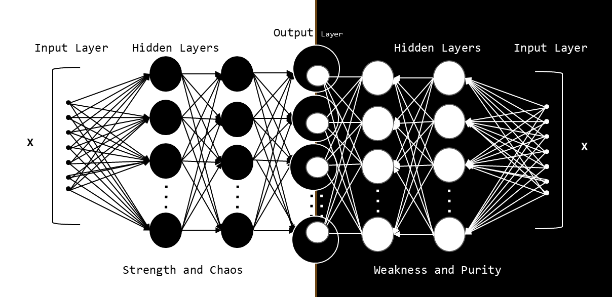
Figure 1: A simple manifestation of an AR framework.

It is important to note that our emphasized viewpoint is that such discrepancies are an endogenous issue that inevitably arises from relative overfitting caused by the model structure. In general circumstances, even LMs with large performance differences possess their respective strengths and weaknesses. Our AR law allows for effectively utilizing these advantages, however slight they seem. This forms the fundamental basis for the general and stable efficacy of our method. Naturally, in extreme cases, such as a model with exceedingly poor performance, the core region we define approximates an empty set, resulting in the SLM’s weight becoming zero, thereby exerting no influence. Specifically, applying softmax to the logit vectors $l_{i}$ ($i=1,2$) output by the two models yields:

$$p_{i}=\mathrm{softmax}(l_{i})$$ (3)

Based on the threshold point of AR, an appropriate weight w (Weights corresponding to the LM) is determined, and a weighted sum is performed to obtain the final output:

$$p_{\text{ensemble}}=w\cdot p_{1}+(1-w)\cdot p_{2}$$ (4)

It can be asserted that an SLM satisfying the threshold point of the AR condition will invariably exert a positive influence on the LLM. This influence is determined by the relative overfitting between the different models, is endogenous, and represents an inevitable outcome of the trade-offs involved. This explains its universal applicability, irrespective of model architecture or performance level. We discuss this point further in the subsequent experimental section, noting that while the magnitude of performance improvement may vary, an enhancement is consistently achievable.

Currently, this method only incurs linear complexity related to vocabulary size when a parallel implementation is considered. In many situations, compared to improving LLM performance by increasing the number of parameters, this training-free method offers significant savings in memory and computation time, particularly for long sequences based on the transformer architecture.

4.2 AR Law

The AR law constitutes the rule within the AR framework that defines the acceptance and rejection criteria for the judgments of various SLMs when operating with a fixed LLM. This chapter will illustrate this based on the ideas, discussions and experimental results of our approach, using the simple implementation of the AR framework described in Section 4.1 as an example.

First, we introduce the concept of the threshold point of AR. Let the parameter ratio between the LLM and the SLM be $k=\frac{|\theta_{\mathrm{LLM}}|}{|\theta_{\mathrm{SLM}}|}$, where $|\theta_{\mathrm{LLM}}|$ denotes the number of parameters in the LLM, and $|\theta_{\mathrm{SLM}}|$ denotes the number of parameters in the SLM. Since the performance of the same model can vary across different datasets, this paper uses parameter count as a proxy for the concept of performance for convenience. Although our discussion uses the parameter ratio as a metric, it is important to note that it represents the performance ratio and the underlying concept of relative overfitting. We define the weight ratio as $\beta=w/(1-w)$. Therefore, if the AR weight allocation ratio that achieves the optimal performance improvement is $\alpha$ ($\alpha$ is designed to maximize the performance improvement of the integrated model $\beta$), then we have:

$$\alpha\propto k$$ (5)

Second, we introduce the concept of the improvement domain, denoted as $[D,\infty]$, where $D<\alpha$. For any weight allocation ratio $\beta$, the model can improve performance when $\beta\in[D,\infty]$. Furthermore, when $\beta<\alpha$, the magnitude of performance improvement increases, and when $\beta>\alpha$, the magnitude of performance improvement decreases. When $\beta=\infty$, it approximates a single model. We also have:

$$R\propto k$$ (6)

When $k$ is extremely large, meaning the performance (parameter) gap between the models is vast, $R$ approaches infinity ($R\to\infty$). In this scenario, we consider the performance improvement to be near zero. Of course, this situation rarely occurs. To verify this extreme case, we designed an experiment using a model with abysmal performance and very high perplexity to construct the AR framework. In this case, the performance improvement was almost negligible.

Finally, the magnitude of performance improvement is inversely proportional to the weight ratio $\beta$.

The points described above constitute the basic AR law, which is defined on the basis of the theoretical ideas presented earlier. Next, we will discuss the selection of the AR threshold point.

4.3 The Threshold Point of AR

Based on the ideas discussed in the previous section, we examine the threshold point of the optimal allocation ratio $\alpha$ based on the experimental results.

We decompose the optimal ratio $\alpha$ into two conflicting components. The first is an ascending component. If the parameter ratio $k$ between the LLM and the SLM is large, we should use a larger $\alpha$ to better utilize the LLM’s capability for detail, essentially its conventionally understood performance. According to Kaplan 1 , LLM performance follows a power law concerning parameter count, suggesting($p$ is the power-law exponent):

$$\alpha\propto k^{p}$$ (7)

The second component characterizes the magnitude at which the AR framework operates effectively. In reality, $k$ only describes the gap between LLM and SLM but does not capture the starting point of this gap. We introduce the parameter $\theta_{LLM}$ (the LLM’s parameter count) to represent the starting point where this influence takes effect. For example, the ratio between parameters 14B, 7B, 14M, and 28M is also 2, but the magnitude of the differences is entirely different. Relative overfitting cases arising from different magnitudes will also vary. Therefore, as noted in Section 4.2, we discuss how to influence it based on the AR framework and law under a fixed LLM. The average optimal weight $\alpha$ of each model in various datasets in all experiments from Section 5.1 is presented in Appendix B.2.

4.4 Improvement Magnitude

In this subsection, we discuss the magnitude of performance improvement contributed by the lower performing model to the higher performing model within the AR framework. Unlike previous discussions, although dependent on weights, the magnitude of performance improvement is influenced by more complex factors in practice than the relatively strict proportional and inverse relationships explored in Section 4.2. Based on the experimental results, we identify two empirical regularities. First, as the weight ratio (associated with the LLM) increases, the proportion and influence of the SLM decrease. However, this inverse relationship is not absolute; exceptions were observed in experiments. This is because the change in proportion is an integral part of the AR law itself: reducing the SLM’s proportion serves the mechanism’s requirements and is not merely about decreasing the SLM’s influence. we see that the actual optimal weight ratio $\alpha$ increases only with $k$ (the parameter ratio). Secondly, as stated in Section 4.3. We observe that while the actual optimal weight ratio $\alpha$ increases with our experiments, it does not demonstrably increase with the scale of the main model parameters $\theta_{LLM}$. This provides evidence for the stability of the AR framework: that is, as long as an appropriate k is maintained, the increase in the model’s performance remains stable with the growth of $\theta_{LLM}$, and in some scenarios, there is even a rising trend (as seen in Section 5.1). This means that, according to the AR law, we need not worry about a significant reduction in performance due to extensive main model parameters. This finding supports our belief that this approach can positively impact the bottleneck observed in scaling laws. Moreover, under the scaling law, as the LLM parameters increase, the rate of improvement decreases rapidly.

4.5 Proof of part of the AR law

Chapters 4.2, 4.3, and 4.4 present empirical conclusions derived from our tens of thousands of experimental results. In fact, we provide a rigorous proof concerning the AR law based on the ACC metric, under specific assumptions, as seen in Appendix A. This proof not only demonstrates a part of the correctness of AR law, but its proof process also more comprehensively illustrates the ideas contained within the AR framework.

5 Experiments

To validate the method proposed in this paper, in the field of NLP, we designed experiments considering existing mainstream scaling-law-based LMs and custom-built LMs based on prevalent architectures. The aim is to verify the universality, effectiveness, stability, and flexibility of our approach. First, we tested our method on several existing scaling law-based model series (e.g., GPT-2 33 ). Second, we performed ablation studies using a model built on the Transformer 31 architecture, deliberately avoiding task-specific design modifications and comparing with existing models. Finally, we retrained models of varying scales based on the mainstream architectures LSTM 29 ; 30 , Transformer, and GRU 32 for further experimentation. This chapter demonstrates that the proposed method is universally applicable to various models, including mainstream models, custom models, and combinations thereof. Furthermore, based on the principle of relative overfitting, we validated the AR framework in computer vision (CV) and AI for science.

5.1 Mainstream Language Model Testing

This paper conducted experiments using the proposed AR framework on several pre-trained models. The tests were performed using GPT-2 33 on fundamental language modeling benchmarks including WikiText2, WikiText103 34 , text8 14 , Pile 39 ; 40 (using a randomly sampled subset of the Pile test set), and 1BW 38 , as well as on the long-context benchmark LAMBADA 35 and the QA benchmarks CBT 36 and the subject examination benchmark ARC 37 . We also evaluated the performance of models with different architectures: Pythia 41 (multiscale scaling law), RWKV 42 (combining RNN and Transformer), Mamba 43 (state-space model series), and Qwen 44 ; 45 (commercial LLM) - using the AR framework for basic language modeling tasks. We used the LAMBADA dataset for the language modeling evaluation (perplexity) and its original long-context dependency evaluation to compare the behavior under the AR framework between general language modeling and specific tasks.

The results in Table 1 demonstrate that all models achieve universal performance improvements through our AR framework. We can achieve superior performance in many scenarios with significantly fewer parameters and less computation time. For instance, on LAMBADA (PPL), Pile, and other benchmarks, our method consistently outperforms the strategy of simply increasing the LLM’s parameter count, achieving superior parameters, computation time, and performance. This advantage becomes more pronounced as the model parameters increase. For example, based on the improvement rate observed when scaling GPT-2 from 762M to 1.5B, and roughly estimating the improvement from 1.5B to 3B using the power law model proposed in scaling laws, the performance of the 1.5B+762M combination almost universally surpasses the projected 3B model across all benchmarks. Notably, our method’s advantages become more significant with larger models, while the linear complexity related to vocabulary size becomes negligible compared to increasing the parameter count. Furthermore, as the main model’s parameters grow, the magnitude of performance improvement increases rather than diminishes, making us optimistic about its performance on even larger models and hopeful that it can contribute to alleviating the scaling law bottleneck.

Table 1: The table shows the test results of the classic model GPT2 based on the AR framework with four parameter sizes from 117M to 1.5B. LTD is the long context benchmark under the LAMBADA dataset. The results of RWKV, Mamba, Pythia, and Qwen can be found in the Appendix D.1.

LLM	SLM	WikiText2	WikiText103	text8	1BW	Pile(part)	LAMBADA	LAMBADA	CBT-CN	CBT-NE	ARC
GPT2	GPT2	PPL $\downarrow$	PPL $\downarrow$	BPC $\downarrow$	PPL $\downarrow$	PLL $\downarrow$	PPL $\downarrow$	PLL(LTD) $\downarrow$	ACC $\uparrow$	ACC $\uparrow$	ACC $\uparrow$
117m		23.52	29.16	1.21	63.97	18.66	43.08	24.99	78.84	72.40	22.35
345m		17.99	21.08	1.10	52.75	13.74	33.66	12.66	82.88	75.36	25.00
762m		15.84	18.15	1.05	45.67	13.20	30.61	9.33	84.68	76.32	24.40
1.5b		14.80	16.51	1.02	43.81	12.15	29.96	7.80	86.92	78.92	26.62
Improvement of the evaluation metric relative to the best performing single model (%)
345m	117m	1.15%	0.62%	0.32%	2.16%	1.11%	1.63%	0.28%	0.24%	2.34%	1.71%
762m	117m	0.77%	0.42%	0.20%	1.15%	4.68%	1.81%	0.01%	0.43%	2.46%	1.40%
762m	345m	2.73%	2.17%	1.00%	2.26%	9.51%	4.13%	1.07%	0.85%	1.52%	3.41%
1.5b	117m	0.82%	0.50%	0.27%	1.52%	4.52%	2.36%	0.12%	0.37%	1.57%	1.28%
1.5b	345m	2.01%	1.47%	0.72%	2.16%	8.41%	4.92%	0.54%	0.18%	0.66%	2.88%
1.5b	762m	3.85%	3.24%	1.38%	4.72%	4.97%	6.99%	3.31%	0.18%	0.61%	1.92%

5.2 Ablation Experiments with Custom-Built Models Based on Mainstream Architectures

In this section, we use the vocabularies corresponding to Pythia, RWKV, Mamba, and GPT-2 to verify the universality and flexibility of our proposed method. Without incorporating any specific design elements, we employed a simple Transformer architecture to train a reference model with only approximately 180M parameters. In practice, the standalone performance of this model is not particularly strong.

We designed a control experiment to further validate the universality, stability, and flexibility of our method. In WikiText103 and LAMBADA datasets, we performed predictions using only the model trained on WikiText2, without using the corresponding training sets for these target datasets. This was done to confirm that the performance improvement achieved by the AR framework is not merely due to having "seen the data". Furthermore, to verify the effectiveness of our method, we trained models on the 1BW and text8 datasets using their respective training sets to achieve substantial performance gains. Training different models (with poor, moderate, and good performance) based on different datasets aims to better observe the relative overfitting and performance of the AR framework under various circumstances. In addition, we will present the results based on the same model in Appendix D.2.

The results in Table 2 indicate that although the models we trained on WikiText2 and WikiText103 did not perform well individually, their magnitudes of improvement exceeded those of the inherently superior but highly homogeneous models. The results on the LAMBADA dataset further demonstrate that even inferior models can still contribute improvements through the AR framework. The results in the text8 and 1BW datasets illustrate that our method is universal and highly effective (even though we did not specifically search for the optimal fulcrum $\alpha$). The AR framework based on non-homogeneous models has nearly achieved comprehensive advantages in computation, parameters, and performance in specific scenarios compared to LLMs that seek improvement by increasing the number of parameters. Even without additional design, enhancements will occur if the AR framework identifies an appropriate threshold point based on relative overfitting.

It is important to note that this is not fine-tuning 46 ; 47 , but merely a training-free bias correction. Compared to fine-tuning, our method offers greater flexibility, requires significantly fewer resources, and does not affect the base model (domain-specific fine-tuning may lead to performance degradation in other domains, as seen with DeepSeekR1 48 ).

Table 2: All models used the simplest Transformer architecture. For WikiText2, WikiText103, and LAMBADA results, models were trained on the WikiText2 training set, while for 1BW and text8 results, models were trained on the 1BW and text8 training sets, respectively.

Model	WikiText2	WikiText103	LAMBADA	text8	1BW
Trained Model	PPL $\downarrow$	PPL $\downarrow$	PPL $\downarrow$	BPC $\downarrow$	PPL $\downarrow$
GPT2-Train	91	322	9084	1.03	131
Other-Train	94	314	12084	1.10	45
Improvement of the evaluation metric relative to the best performing single model (%)
GPT2-1.5b	9.46%	6.33%	1.02%	26.12%	22.40%
Pythia-2.8b	3.76%	3.09%	0.10%	19.61%	47.74%
Mamba-2.8b	4.26%	3.56%	0.10%	18.68%	45.71%
RWKV-1.5b	4.64%	3.67%	0.08%	20.53%	49.02%

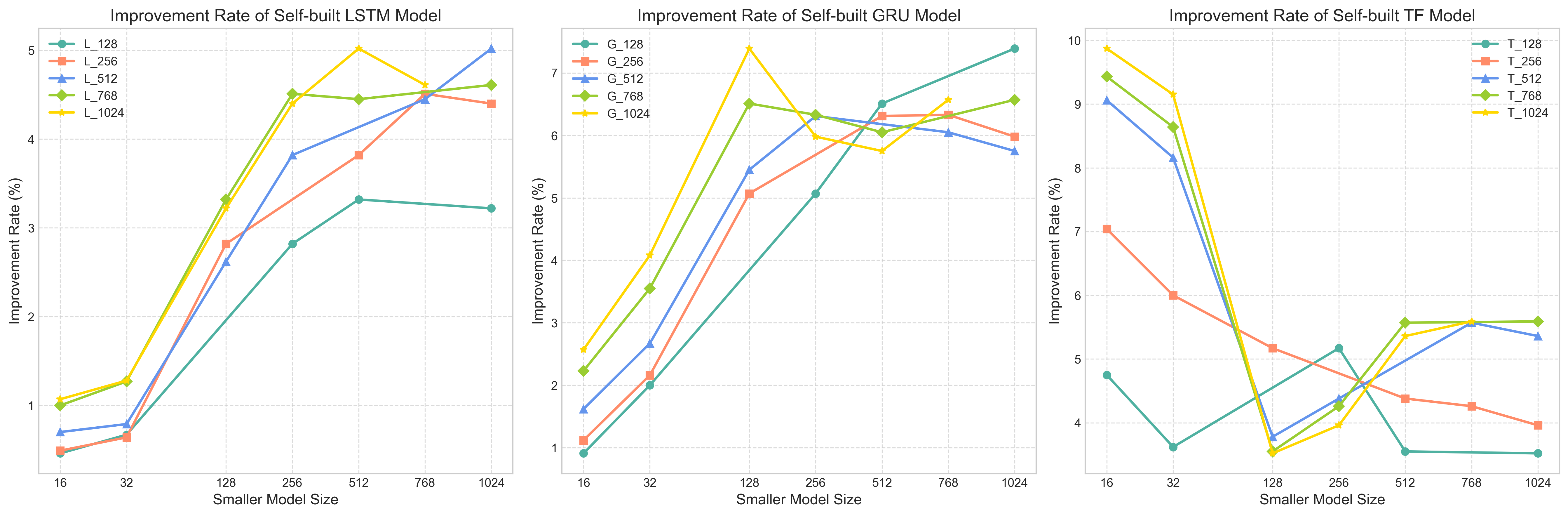
Figure 2: Test results of AR framework based on simple LSTM, Transformer and GRU architectures under different embedding dimensions of SLM and LLM.

5.3 Self-built model testing based on mainstream architectures

This paper conducted tests based on the current mainstream model architectures LSTM 29 ; 30 , Transformer 31 , and GRU 32 , utilizing the same vocabulary but varying embedding dimensions. In practice, we used very simple architectures 49 ; 50 ; 51 ; 52 without any specific modifications to the model design. Our method demonstrates universal and stable effectiveness (as illustrated in Figure 2).

5.4 Experiments in the rest of the machine learning field

Based on the principles of relative overfitting and the AR framework, we employed a similar methodology to conduct experiments with our approach across a broader range of machine learning domains, including CV and AI for Science, thus validating the general effectiveness of our proposed framework. We conducted experiments using different sizes of ResNet64 models and ESM65 models on image classification and protein sequence prediction tasks (in the Appendix C).

6 Discussion and Future work

We discuss limitations and future directions.

• Model Selection Trade-offs: For homogeneous scaling models, while performance showed stability (no significant fluctuations) as the main model grew, the magnitude of improvement decreased as the parameter ratio expanded. Larger ratios required more extreme leverage, reducing the effectiveness of SLM and potentially limiting resource savings. In specific domains, nonhomogeneous models are a better choice.

• Better Improvement Magnitude: Although this paper proposes the AR law based on relative overfitting and demonstrates its universal, stable, and practical improvements along with good flexibility under a suitable threshold point, significant room for progress remains beyond the decent performance improvements already achieved. To reveal fundamental principles, our method achieved these results despite lacking any specific model design, highlighting the potential yet to be unlocked. Therefore, with a deeper understanding of the entire system and relative overfitting, key research questions worth exploring include different combination methods based on the AR law, the selection and innovation of low-parameter reference model architectures serving as backbones, and how to maintain the information purity of the SLM better. We anticipate that addressing these questions will lead to greater magnitudes of improvement.

• Limitations of the AR law: As noted in this paper, the AR framework involves complex relative overfitting. Although we have proposed fundamental principles applicable in most scenarios, the inherent black-box nature and uncertainty of neural networks mean that minor fluctuations can occur within the general direction established by the AR Law. Consequently, we believe that the complex influence mechanisms of relative overfitting warrant further in-depth research.

• Broader Applicability: Although this paper focuses mainly on the NLP domain and has also conducted some experiments in CV and AI for science, a broader discussion in more fields was not feasible due to limited time and resources. The applicability of the relative overfitting phenomenon and the proposed AR framework in a broader range of domains warrants further exploration.

Appendix

A Proof of Theorem

A.1 Definitions

Definition A.1.1.

Let $q$ and $q^{\prime}$ be two models sharing the same input and output spaces. If model $q$ has a larger number of parameters (or higher model complexity) than model $q^{\prime}$, we define $q$ as the Large Model (LM) and $q^{\prime}$ as the Small Model (SM).

Definition A.1.2.

Let $S$ be the set of all samples (or positions) to be predicted in a given task, its size being $N=|S|$. Let $s\in S$ represent a specific sample. Let $V=\{1,2,3,\dots,|V|\}$ be the set of indices for all possible output classes (dimensions), where the output dimensions of the two models correspond one-to-one.

Definition A.1.3.

Let $k_{s}\in V$ be the index of the true class for sample $s$. Let $q_{s}$ be the predicted output vector of model $q$ for sample $s$.

Definition A.1.4.

Let $q_{s,i}$ be the probability assigned by model $q$ to sample $s$ belonging to class $i$. Similarly, $q^{\prime}_{s,i}$ is defined for model $q^{\prime}$.

Definition A.1.5.

Model $q$ predicts sample $s$ correctly if and only if $\arg\max_{i\in V}(q_{s,i})=k_{s}$.

Definition A.1.6.

The entire set of samples in the task is partitioned into three sets: $T$, $F$, and $N$.

• The set $T$ consists of samples where the LM predicts incorrectly, but the SM predicts correctly:

  $$T=\{s\in S\mid\arg\max_{i\in V}(q_{s,i})\neq k_{s}\text{ and }\arg\max_{i\in V}(q^{\prime}_{s,i})=k_{s}\}$$

• The set $F$ consists of samples where the LM predicts correctly, but the SM predicts incorrectly:

  $$F=\{s\in S\mid\arg\max_{i\in V}(q_{s,i})=k_{s}\text{ and }\arg\max_{i\in V}(q^{\prime}_{s,i})\neq k_{s}\}$$

• The set $N$ consists of samples where both LM and SM predict correctly, or both predict incorrectly.

We have $T\cup F\cup N=S$, and $T,F,N$ are mutually disjoint.

Definition A.1.7.

The accuracy (ACC) of a model on a prediction task $S$ is defined as (where $I(\cdot)$ is the indicator function):

$$ACC_{q}=\frac{1}{|S|}\sum_{s\in S}I(\arg\max_{i\in V}(q_{s,i})=k_{s})$$

A.2 Assumptions and Core Theorems

Assumption A.2.1.

The improvements of larger models are primarily concentrated in the tail of the distribution. Assume there exists a high-frequency output class $h\in V$. Let $S_{h}^{q}=\{s\in S\mid\arg\max_{i}q_{s,i}=h\}$ be the set of samples predicted as $h$ by LM, with size $n=|S_{h}^{q}|$. Let $S_{h}^{q^{\prime}}=\{s\in S\mid\arg\max_{i}q^{\prime}_{s,i}=h\}$ be the set of samples predicted as $h$ by SM, with size $m=|S_{h}^{q^{\prime}}|$.

We assume the following conditions hold53 ; 54 ; 55 ; 56 ; 57 ; 58 :

1. The SM outputs class $h$ more frequently than the LM, i.e., $n<m$.

2. The advantage of LM’s prediction accuracy for class $h$, $P_{L}(h)=P(k_{s}=h\mid s\in S_{h}^{q})$, over SM’s accuracy, $P_{S}(h)=P(k_{s}=h\mid s\in S_{h}^{q^{\prime}})$, is limited. Specifically, this advantage satisfies the relation:

   $$|P_{L}(h)-P_{S}(h)|<\frac{(m-n)P_{S}(h)}{n}$$

Theorem A.2.2 (Mainstay Deviation).

Under Assumption A.2.1, for class $h$, the total number of correct predictions by SM is greater than that by LM.

Proof.

The total number of correct predictions for class $h$ by LM is $N_{L}^{h}=n\cdot P_{L}(h)$. The total number of correct predictions for class $h$ by SM is $N_{S}^{h}=m\cdot P_{S}(h)$.

We want to prove $N_{L}^{h}<N_{S}^{h}$, which is equivalent to proving $m\cdot P_{S}(h)-n\cdot P_{L}(h)>0$.

We transform the difference:

$$m\cdot P_{S}(h)-n\cdot P_{L}(h) =m\cdot P_{S}(h)-n\cdot P_{S}(h)+n\cdot P_{S}(h)-n\cdot P_{L}(h)$$

$$=(m-n)P_{S}(h)-n(P_{L}(h)-P_{S}(h))$$

From Assumption A.2.1, we have:

$$(P_{L}(h)-P_{S}(h))\leq|P_{L}(h)-P_{S}(h)|<\frac{(m-n)P_{S}(h)}{n}$$

Thus,

$$(m-n)P_{S}(h)-n(P_{L}(h)-P_{S}(h))>(m-n)P_{S}(h)-n\left(\frac{(m-n)P_{S}(h)}{n}\right)=0$$

The inequality is proven.

It can be easily shown that Theorem A.2.2 holds for any high-frequency output dimension satisfying Assumption A.2.1. ∎

Lemma A.2.3 (Exchange Condition).

Let the fused model be $q_{new,s,i}=w\cdot q_{s,i}+(1-w)\cdot q^{\prime}_{s,i}$ for $w\in(0,1)$. On sample $s$, if the LM’s original prediction is $i$ (i.e., $\arg\max(q_{s})=i$), for the fused model’s prediction for class $j$ to have a higher probability than for class $i$, it must satisfy:

$$w\cdot q_{s,j}+(1-w)\cdot q^{\prime}_{s,j}>w\cdot q_{s,i}+(1-w)\cdot q^{\prime}_{s,i}$$

For $w\in(0,1)$, this inequality is equivalent to:

$$\frac{q_{s,i}-q_{s,j}}{q^{\prime}_{s,j}-q^{\prime}_{s,i}}<\frac{1-w}{w}$$

Clearly, we need SM’s prediction for $j$ to be greater than its prediction for $i$:

$$q^{\prime}_{s,j}-q^{\prime}_{s,i}>0$$

This is termed the exchange condition.

Furthermore, if $\arg\max(q_{new,s})=j$, then the fused model’s prediction changes from $i$ to $j$. This is termed the strict exchange condition if the exchange condition is also met.

We define the left side as the Exchange Threshold, denoted $ET(s,i\to j)$. A flip occurs only when $ET<\frac{1-w}{w}$.

This lemma implies that only when the exchange condition is met can the fused model’s prediction potentially differ from the LM’s prediction. Any case not satisfying this condition cannot change the prediction outcome. Moreover, only when the strict exchange condition is met can the change in prediction outcome be determined.

Assumption A.2.4 (Stratification of Predictions).

Typically, a model exhibits greater discrimination for samples it predicts correctly68 ; 69 ; 70 . Specifically, we assume situations exist where: for some samples correctly predicted by model $q$ (e.g., $b\in F$), the difference between the probability of the correctly predicted class $q_{b,k_{b}}$ and the probability of the second most likely class (or any other incorrect class $x_{b}$, $q_{b,x_{b}}$), i.e., $(q_{b,k_{b}}-q_{b,x_{b}})$, is greater than the difference for some samples incorrectly predicted by model $q$ (e.g., $a\in T$) between its incorrectly predicted class probability $q_{a,i_{a}}$ and the true class probability $q_{a,k_{a}}$ (or some other reference class $z_{a}$, $q_{a,z_{a}}$), i.e., $(q_{a,i_{a}}-q_{a,z_{a}})$.

Formally, there exists at least one sample $a\in T$ such that for all samples $b\in F$ (if $F$ is non-empty):

$$(q_{b,k_{b}}-\max_{j\neq k_{b}}q_{b,j})>(q_{a,i_{a}}-q_{a,k_{a}})$$

where $k_{b}=\arg\max(q_{b})$ is LM’s correct prediction for $b$, $i_{a}=\arg\max(q_{a})$ is LM’s incorrect prediction for $a$, and $k_{a}$ is the true class of $a$.

A similar condition holds for model $q^{\prime}$:

$$(q^{\prime}_{b,k_{b}}-\max_{j\neq k_{b}}q^{\prime}_{b,j})>(q^{\prime}_{a,i^{\prime}_{a}}-q^{\prime}_{a,k_{a}})$$

Let $A$ be the set of all samples $a\in T$ satisfying this condition.

Theorem A.2.5 (AR Law: Improvement, Not Degradation).

We say Condition (1) holds if there exists a position $s\in S$ where SM’s predictive capability is stronger than LM’s. Specifically, LM predicts incorrectly, $k_{s}\neq\arg\max(q_{s})$, and SM’s predicted probability for the true class $k_{s}$ is greater than its predicted probability for LM’s incorrect prediction $i_{s}=\arg\max(q_{s})$, i.e., $q^{\prime}_{s,k_{s}}>q^{\prime}_{s,i_{s}}$. (From Theorem A.2.2 and experimental results, this condition is generally met.)

Under Assumption A.2.4: For a linear fusion model $q_{new}=w\cdot q+(1-w)\cdot q^{\prime}$ (where $w\in(0,1)$) of a large model $q$ and a small model $q^{\prime}$, if and only if Condition (1) holds, a weight $w$ can always be found such that the accuracy of the fused model $ACC_{new}$ is potentially higher than, and not worse than, the accuracy of model $q$, i.e., $ACC_{new}\geq ACC_{q}$.

If, additionally, for the set $A$, there exists at least one position satisfying the strict exchange condition, then the accuracy of the fused model $ACC_{new}$ is higher than the accuracy of model $q$, i.e., $ACC_{new}>ACC_{q}$. In fact, for every predicted position $s$, the conclusion is that the accuracy will not decrease.

Proof.

From Lemma A.2.3, for the weighted output to potentially differ, the exchange condition must be met. For $\arg\max(q_{s})=i$:

$$w\cdot q_{s,j}+(1-w)\cdot q^{\prime}_{s,j}>w\cdot q_{s,i}+(1-w)\cdot q^{\prime}_{s,i}$$

For output $j$ to replace output $i$ as the final output, it is also required that:

$$\arg\max(w\cdot q_{s}+(1-w)\cdot q^{\prime}_{s})=j$$

Assume Condition (1) does not hold. Then for any position $s\in S$: If $q_{s,i}=\arg\max(q_{s})=k_{s}$, then $q$ is already optimal at this position, and fusion can only lead to a worse result. If $q_{s,i}=\arg\max(q_{s})\neq k_{s}$, but $q^{\prime}_{s,k_{s}}<q^{\prime}_{s,i_{s}}$ (where $i_{s}$ is the LM’s incorrect prediction), then

$$w\cdot q_{s,k_{s}}+(1-w)\cdot q^{\prime}_{s,k_{s}}<w\cdot q_{s,i_{s}}+(1-w)\cdot q^{\prime}_{s,i_{s}}$$

This means the true class $k_{s}$ can never replace the LM’s incorrect prediction $i_{s}$ as the final output. Thus, the necessity of Condition (1) is proven.

Consider the partition of the task into sets $T,F,N$. Let $t\in T$ and $f\in F$. For set $N$: if both models predict correctly, the weighted result cannot change the original $\arg\max$. If both predict incorrectly, the result cannot worsen. Thus, for set $N$, weighting can only potentially improve ACC.

For set $T$: if the exchange condition $\frac{q_{t,i_{t}}-q_{t,k_{t}}}{q^{\prime}_{t,k_{t}}-q^{\prime}_{t,i_{t}}}<\frac{1-w}{w}$ (where $i_{t}$ is LM’s incorrect prediction and $k_{t}$ is the true class) is met, the incorrect result $i_{t}$ can be replaced by the correct result $k_{t}$.

For set $F$: if the exchange condition $\frac{q_{f,k_{f}}-q_{f,j_{f}}}{q^{\prime}_{f,j_{f}}-q^{\prime}_{f,k_{f}}}<\frac{1-w}{w}$ (where $k_{f}$ is LM’s correct prediction and $j_{f}$ is SM’s incorrect prediction) is met, the true result $k_{f}$ can be replaced by an incorrect result $j_{f}$, causing ACC to decrease.

By Assumption A.2.4, there exists some $a\in A\subseteq T$ such that for all $f\in F$:

$$(q_{f,k_{f}}-\max_{j\neq k_{f}}q_{f,j})>(q_{a,i_{a}}-q_{a,k_{a}})$$

and

$$(q^{\prime}_{a,k_{a}}-q^{\prime}_{a,i^{\prime}_{a}})>(q^{\prime}_{f,j_{f}}-q^{\prime}_{f,k_{f}})$$

This implies that the exchange threshold for correcting $a$ is smaller than the exchange threshold for incorrectly changing $f$:

$$\frac{q_{a,i_{a}}-q_{a,k_{a}}}{q^{\prime}_{a,k_{a}}-q^{\prime}_{a,i_{a}}}<\frac{q_{f,k_{f}}-q_{f,j_{f}}}{q^{\prime}_{f,j_{f}}-q^{\prime}_{f,k_{f}}}$$

At this point, we can always find a $w$ such that:

$$\frac{q_{a,i_{a}}-q_{a,k_{a}}}{q^{\prime}_{a,k_{a}}-q^{\prime}_{a,i_{a}}}<\frac{1-w}{w}<\frac{q_{f,k_{f}}-q_{f,j_{f}}}{q^{\prime}_{f,j_{f}}-q^{\prime}_{f,k_{f}}}$$

Since $a\in T$, this means that a potential correct substitution in set $T$ is satisfied, while an incorrect substitution in set $F$ is not. Thus, ACC may increase and cannot decrease.

If there is at least one point $a^{\prime}\in A$ that satisfies the strict exchange condition, then at this position, the incorrect result will be replaced by the correct result, causing an increase in ACC. There are N additional episodes that will not cause a decline in accuracy, thus there exists a w such that at any prediction position s, accuracy will not decrease. ∎

Theorem A.2.6 (AR Law: Maximum Improvement Magnitude).

Under the conditions of Theorem A.2.5, let $A$ be the set of all positions satisfying Assumption A.2.4. Let $R$ be the set of all positions satisfying the strict exchange condition, where $R\subseteq A\subseteq T\subseteq S$. The accuracy improvement $\Delta ACC=ACC_{new}-ACC_{q}$ of the fused model $q_{new}$ relative to the original large model $q$ has the following properties:

• $\Delta ACC$ is a strictly monotonically increasing function of the size of set $R$, $|R|$.

• $\Delta ACC$ is a monotonically increasing function of the sizes of sets $A$ and $T$, $|A|$ and $|T|$.

Proof.

According to Theorem A.2.5, by choosing an optimal fusion weight $w$, we can ensure that only samples in set $T$ are corrected, and samples in set $F$ are not incorrectly changed.

By definition, $R$ is the set of all samples that can be safely corrected within the optimal weight range. Then, the maximum accuracy improvement $\Delta ACC_{max}$ directly depends on the size of $R$:

$$\Delta ACC_{max}=\frac{|R|}{|S|}$$

From this equation, it is clear that if $|R|$ increases, $\Delta ACC_{max}$ will also increase proportionally. Therefore, $\Delta ACC_{max}$ is a strictly monotonically increasing function of $|R|$.

By definition, we have the subset relations $R\subseteq A\subseteq T$. This directly leads to the inequality relations for set sizes: $|R|\leq|A|\leq|T|$. Therefore, the maximum accuracy improvement is limited by $|A|$ and $|T|$:

$$\Delta ACC_{max}=\frac{|R|}{|S|}\leq\frac{|A|}{|S|}\leq\frac{|T|}{|S|}$$

This inequality shows that the upper limit of ACC improvement is determined by $|A|$ and $|T|$.

Now consider monotonicity. If set $A_{1}\subseteq A_{2}$, then the correctable sets extracted from them also satisfy $R(A_{1})\subseteq R(A_{2})$. Therefore, $\Delta ACC_{max}(A_{1})\leq\Delta ACC_{max}(A_{2})$. This means $\Delta ACC_{max}$ is a monotonically increasing (non-decreasing) function of $|A|$.

By the same logic, since $A\subseteq T$, $\Delta ACC_{max}$ is also a monotonically increasing (non-decreasing) function of $|T|$. ∎

Theorem A.2.7 (AR Law: ACC Improvement Variation with Weight).

Building on Theorem A.2.5, let $\beta=w/(1-w)$. As the weight $w$ decreases (and thus $\beta$ decreases, while $(1-w)/w$ increases), the ACC improvement magnitude initially increases monotonically.

If for any $r\in R$, Assumption A.2.4 is satisfied (implying $R=A=T$ under ideal conditions), then there exists an optimal weight range where $\beta=\alpha$ such that the ACC improvement reaches its maximum. Subsequently, as $w$ further decreases ( $\beta$ further decreases), the ACC improvement magnitude monotonically decreases, until $\beta=D$, after which ACC begins to decline (That is, the lifting domain of ACC is $[D,\infty]$).

Proof.

From Theorem A.2.5, we have the condition for favorable exchange:

$$\frac{q_{a,i_{a}}-q_{a,k_{a}}}{q^{\prime}_{a,k_{a}}-q^{\prime}_{a,i_{a}}}<\frac{1-w}{w}<\frac{q_{f,k_{f}}-q_{f,j_{f}}}{q^{\prime}_{f,j_{f}}-q^{\prime}_{f,k_{f}}}$$

Let $A^{\prime}$ be the set of points satisfying $\frac{q_{a,i_{a}}-q_{a,k_{a}}}{q^{\prime}_{a,k_{a}}-q^{\prime}_{a,i_{a}}}<\frac{1-w}{w}$ and also satisfying the strict exchange condition. It is clear that the current ACC improvement is proportional to $|A^{\prime}|$, and $A^{\prime}\subseteq R$.

With $A$ (and thus $R$) fixed, as $w$ decreases, $\beta=w/(1-w)$ decreases, and $\tau=(1-w)/w$ increases. As $\tau$ increases, more samples in $R$ will satisfy $ET<\tau$, so $|A^{\prime}|$ monotonically increases. Consequently, the ACC improvement magnitude increases.

If $R=A=T$ (ideal case where all potential corrections satisfy Assumption A.2.4), then when $|A^{\prime}|=|R|$ (all samples in $R$ are corrected), the ACC improvement reaches its maximum. At this point, let the corresponding $\beta$ be $\alpha$.

As $w$ continues to decrease ( $\beta$ continues to decrease, $\tau$ continues to increase), $|A^{\prime}|$ no longer increases (it is capped at $|R|$). Now, $R=T=A^{\prime}$. The increase in $\tau$ will only cause more samples in $F$ to satisfy

$$\frac{q_{f,k_{f}}-q_{f,j_{f}}}{q^{\prime}_{f,j_{f}}-q^{\prime}_{f,k_{f}}}<\frac{1-w}{w}$$

Let $B$ be the set of these positions from $F$. For $f\in B$, an incorrect prediction $j_{f}$ by SM replaces the correct LM prediction $k_{f}$, causing the ACC improvement magnitude to decrease (i.e., net ACC starts to fall).

When $|B|$ (number of newly incorrect predictions) becomes greater than $|R|$ (number of correct predictions that were maintained or newly made), the net change in ACC becomes negative, meaning ACC starts to decline rather than improve. We define the weight ratio $\beta$ at which this first occurs as $D$. ∎

A.3 Corollaries

Corollary A.3.1 (Multi-dimensional Extension).

The conclusions of the AR Law (Theorems A.2.5, A.2.6, A.2.7) hold for any dimension of the output vector. In other words, the validity of these laws does not depend on the total number of dimensions in the output space.

Proof.

We use mathematical induction on the total number of output dimensions $D_{dim}=|V|$.

Base Case: When $D_{dim}=2$, the problem is a binary classification. The LM’s prediction $i$ and SM’s prediction $k$ (if different) are the only two classes. All comparisons regarding Exchange Thresholds (ET) and prediction stratification (Assumption A.2.4) are made directly on these two dimensions. The logic and derivations of Theorems A.2.5, A.2.6, A.2.7 hold directly in this simplest case.

Inductive Hypothesis: Assume that for any output space of dimension $D_{dim}-1$ (where $D_{dim}>2$), the AR Law holds.

Inductive Step: We need to prove that under this assumption, the AR Law also holds for an output space of dimension $D_{dim}$.

Consider a $D_{dim}$-dimensional output space $V$. The core mechanism of the AR Law, i.e., the change in prediction of the fused model $q_{new}$, depends on the exchange condition in Lemma A.2.3. For example, for the prediction to flip from class $i$ to class $j$, it must satisfy:

$$w\cdot q_{s,j}+(1-w)\cdot q^{\prime}_{s,j}>w\cdot q_{s,i}+(1-w)\cdot q^{\prime}_{s,i}$$

Rearranging gives the condition for the exchange threshold:

$$\frac{q_{s,i}-q_{s,j}}{q^{\prime}_{s,j}-q^{\prime}_{s,i}}<\frac{1-w}{w},\quad\text{where }q^{\prime}_{s,j}>q^{\prime}_{s,i}$$

Crucially, this core condition for flipping only involves the probabilities of these two dimensions, $i$ and $j$, and is independent of the probability values of any other dimension $u\in V\setminus\{i,j\}$.

Now, let us arbitrarily remove one dimension $u$ from the $D_{dim}$-dimensional space, forming a $(D_{dim}-1)$-dimensional subspace $V^{\prime}=V\setminus\{u\}$. We can construct a new classification subproblem defined on $V^{\prime}$. For this subproblem, we can define a new set of probability distributions normalized over $V^{\prime}$ to determine which class to output.

Importantly, for any two dimensions still in $V^{\prime}$ (e.g., $i$ and $j$), their relative probability magnitudes in the original models $q$ and $q^{\prime}$, and the value of the exchange threshold $ET(s,i\to j)$ calculated from them, are independent of whether we consider dimension $u$.

Therefore, in this $(D_{dim}-1)$-dimensional subspace $V^{\prime}$, all prerequisites of the AR Law (such as Assumptions A.2.1 and A.2.4) and core mechanisms (such as Lemma A.2.3) apply equally. Hence, the AR Law holds for this $(D_{dim}-1)$-dimensional subproblem.

Since the removed dimension $u$ was chosen arbitrarily, this implies that the intrinsic logic of the AR Law holds on any subset of dimensions. Thus, the validity of the law is not restricted to a specific number of dimensions; it naturally extends from $D_{dim}-1$ dimensions to $D_{dim}$ dimensions.

By induction, the AR Law holds for any output space of dimension $D_{dim}\geq 2$.

Specifically, if the removed dimension is the output dimension of the fused model itself at that position, the output changes according to the AR Law. If not, the output at this position does not change. ∎

Corollary A.3.2 (Variant based on Assumption A.2.4).

If, in set $T$, the number of positions satisfying Assumption A.2.4 and the strict exchange condition (denoted as set $R$) is greater than the number of positions not satisfying Assumption A.2.4 (denoted as $T\setminus A$), i.e., $|R|>|T\setminus A|$, then Theorem A.2.5 and Theorem A.2.6 still hold.

Proof.

The goal of this proof is to find a fusion weight $w$ that achieves a net improvement in accuracy under the condition that Assumption A.2.4 does not fully hold, by utilizing the premise $|R|>|T\setminus A|$.

The core challenge is that "risky" samples $a^{\prime}\in T\setminus A$ might have an exchange threshold $ET(a^{\prime})$ greater than the exchange threshold $ET(f)$ of some samples $f\in F$, which means the threshold separation relied upon in the proof of Theorem A.2.5 is no longer absolutely guaranteed.

However, the premise $|R|>|T\setminus A|$ allows us to adopt a conservative strategy to mitigate this risk. We can construct a safe benign sample subset $R_{safe}\subseteq R$, with its size defined as $|R_{safe}|=|R|-|T\setminus A|$.

According to the premise, this subset contains at least one element. Since all elements of $R_{safe}$ are from $R$, they must satisfy Assumption A.2.4. Therefore, for any $r\in R_{safe}$ and $f\in F$, their exchange thresholds satisfy $ET(r)<ET(f)$. This property ensures that the exchange thresholds of all samples in $R_{safe}$ are strictly smaller than the exchange thresholds of all samples in $F$.

Thus, we can always choose a weight ratio $\tau=\frac{1-w}{w}$ such that it falls between the threshold ranges of these two sets, i.e., satisfying $\max_{r\in R_{safe}}\{ET(r)\}<\tau<\min_{f\in F}\{ET(f)\}$.

For a weight $w$ satisfying this condition, all samples in $R_{safe}$ will be successfully corrected, yielding an accuracy gain of at least $\frac{|R_{safe}|}{|S|}>0$, while ensuring that samples in set $F$ are not incorrectly changed, resulting in zero loss. Thus, the accuracy of the fused model achieves a net improvement, proving that Theorem A.2.5 still holds under this variant condition.

The proof for Theorem A.2.6 is then evident. ∎

Corollary A.3.3 (With SM as the Primary Model).

All the preceding theorems are proven with the LM as the primary model, which is generally due to LM having higher ACC than SM.

If the opposite situation occurs, where the small model $q^{\prime}$ has higher accuracy than the large model $q$, then by swapping the roles of the two models, and under the satisfaction of the assumptions, it can similarly be proven that there exists a fusion weight $w$ such that the accuracy of the fused model is higher than that of the original SM model $q^{\prime}$.

Proof.

The proof of this corollary is based on the principle of symmetry. When we consider the more accurate small model $q^{\prime}$ as the primary model and $q$ as the auxiliary model, we aim to prove that the accuracy of the fused model can exceed that of $q^{\prime}$.

To do this, we need to redefine the sets $T$ and $F$ that form the basis of the theory. The new set $T^{\prime}$, i.e., positions where the primary model ($q^{\prime}$) predicts incorrectly and the auxiliary model ($q$) predicts correctly, is defined identically to the original set $F$. Similarly, the new set $F^{\prime}$, i.e., positions where the primary model ($q^{\prime}$) predicts correctly and the auxiliary model ($q$) predicts incorrectly, is defined identically to the original set $T$.

Therefore, swapping roles in the proof process is equivalent to systematically interchanging $T\leftrightarrow F$ in the original proofs. Considering that the mathematical structure of the linear fusion model $q_{new}$ and the calculation of its exchange threshold are inherently symmetrical with respect to $q$ and $q^{\prime}$, we can conclude that by performing the aforementioned symmetrical substitutions of roles, sets, and assumptions, the proof chains of all theorems remain unchanged. ∎

A.4 Concluding Remarks

Theorems A.2.5, A.2.6, and A.2.7 are collectively termed the AR Law. It reveals the principles governing how the accuracy of a fused model changes under certain assumptions. We have observed in tens of thousands of experiments that these laws hold, and combined with some existing research findings, we believe the assumptions of the AR Law are generally valid.

In fact, from the above theorems, it can be seen that the main issues of the AR framework are twofold: finding a method to measure the difference in judgment between two models, and introducing a quantity that reflects our prior judgment of the capabilities of the two models to measure when the difference reaches a threshold for "Accept" and "Reject". This allows us to accept good changes and reject bad ones. In the method described above, this is achieved through probabilities to reflect judgment differences, and the weight $w$ (or $\beta$) reflects the prior judgment.

What we demonstrate in the appendix is the difference in judgments reflected through similarity, and the a priori judgment expressed through the exponent $p$. According to our experimental observations, the methods in the appendix based on the AR framework are also strictly in accordance with the AR law we proposed.

B Discussion and experiments in Chapters Three and Four.

B.1 Larger models have more optional tokens

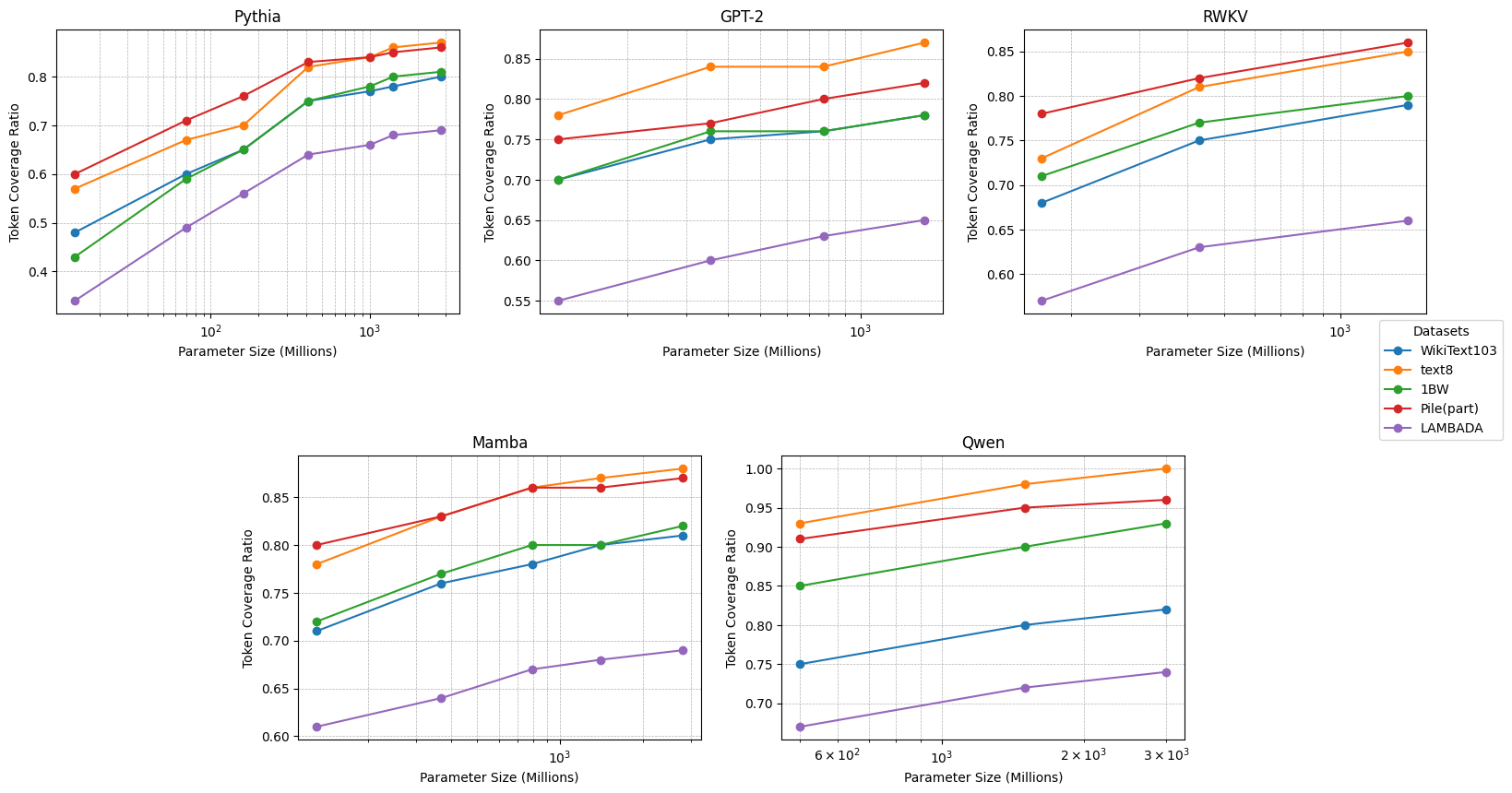
Figure 3: Proportion of tokens generated by scaling law model with different parameters to the total tokens of the dataset under different datasets.

The number of tokens that the model may generate across all datasets increases with the increase in the model parameters.

B.2 Variation of Optimal Weight Ratio $\alpha$ with Parameter Ratio $k$

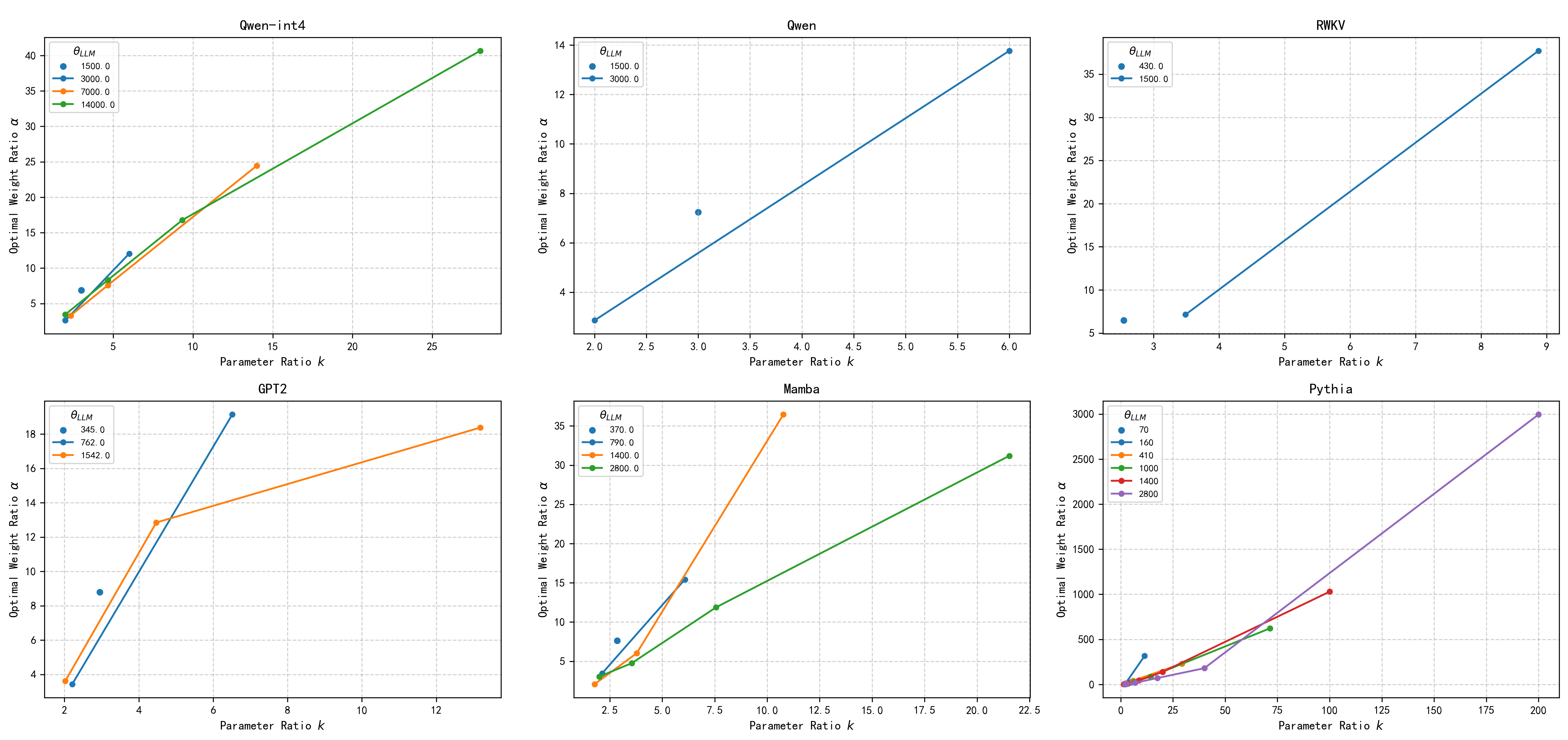
Figure 4: Variation of Optimal Weight Ratio $\alpha$ with Parameter Ratio $k$ for Fixed Main Parameter $\theta_{LLM}$.

Figure 4 shows that under the condition of the same main parameters $\theta_{LLM}$, the optimal weight ratio $\alpha$ for each model shows an increasing trend with increasing parameter ratio.

B.3 AR framework based on cosine similarity

As discussed in the main text, the AR framework emphasizes measuring judgment differences between models and integrating relative overfitting information. Here, we present an alternative approach that, although not entirely successful, provides valuable insights into relative overfitting and the AR law.

We extract the embedding spaces from two models and compute the cosine similarity between each pair of tokens, storing these values for efficient retrieval during inference (see Algorithm1). We prioritize the LLM’s output during inference while using the SLM as a reference. Specifically, we obtain the probability distribution from the LLM and identify the token with the highest probability from the SLM. We then retrieve the cosine similarity vector between each token in the LLM’s vocabulary and the SLM’s highest probability token. Since these similarity values do not form a strict probability space as in our primary method, we employ element-wise multiplication to combine this similarity vector with the LLM’s output probabilities. To incorporate the relative overfitting information, we introduce a hyperparameter $p$ as the power exponent for the similarity vector (Algorithm2).

Algorithm 1 Computing Cosine Similarity Matrix

1:model, chunkSize

2:packedData, metadata

3:$\triangleright$ $E$: Embedding matrix, $V$: Vocabulary size, $S$: Similarity matrix

4:$E\leftarrow\text{ExtractEmbeddings}(model)$

5:$E_{norm}\leftarrow\frac{E}{\|E\|_{2}}$ $\triangleright$ Normalize embeddings

6:$V\leftarrow E_{norm}.\text{shape}[0]$

7:$S\leftarrow\text{zeros}(V,V)$

8:Compute similarity matrix by iterating through chunks:

9:for $i\leftarrow 0$ to $V-1$ step chunkSize do

10:  for $j\leftarrow i$ to $V-1$ step chunkSize do

11:   $S_{chunk}\leftarrow E_{i}\cdot E_{j}^{T}$

12:   if $i=j$ then

13:     $S[i:i+chunkSize,i:i+chunkSize]\leftarrow\text{upperTriangular}(S_{chunk})$

14:   else

15:     $S[i:i+chunkSize,j:j+chunkSize]\leftarrow S_{chunk}$

16:   end if

17:  end for

18:end for

19:$S_{quant}\leftarrow\lfloor S\cdot 15\rfloor$ $\triangleright$ Quantize to 4-bit representation

20:return PackUpperTriangular$(S_{quant})$ $\triangleright$ Store in compressed format

Algorithm 2 Similarity-Based Model Fusion

1:$model_{1}$, $model_{2}$, input, packedData, metadata, $p$ (power law hyperparameter)

2:Ensemble prediction probabilities

3:$\triangleright$ $L$: Logits, $P$: Probabilities, $T$: Token indices, $S$: Similarity matrix

4:$S\leftarrow\text{UnpackUpperTriangular}(packedData,metadata)$ $\triangleright$ Decompress similarity matrix

5:$L_{1}\leftarrow model_{1}(input)$

6:$L_{2}\leftarrow model_{2}(input)$ $\triangleright$ Obtain logits from both models

7:$flat\_L_{1}\leftarrow\text{reshape}(L_{1},[-1,V])$

8:$flat\_L_{2}\leftarrow\text{reshape}(L_{2},[-1,V])$

9:$T_{2}\leftarrow\arg\max(flat\_L_{2},\text{dim}=1)$ $\triangleright$ Identify model 2’s predicted tokens

10:$simWeights\leftarrow S[:,T_{2}]^{p}$ $\triangleright$ Calculate similarity weights with power scaling

11:$P_{1}\leftarrow\text{softmax}(flat\_L_{1},\text{dim}=1)$

12:$P_{ensemble}\leftarrow P_{1}\odot simWeights$ $\triangleright$ Fuse probabilities using similarity weights

13:$P_{ensemble}\leftarrow\frac{P_{ensemble}}{\sum P_{ensemble}}$ $\triangleright$ Re-normalize to ensure valid probabilities

14:return $P_{ensemble}$

This approach is considered less successful because, despite implementing various optimization techniques, the storage requirements for the similarity matrix remain substantial without yielding performance improvements—in fact, it slightly underperforms compared to the method described in the main text. Furthermore, this approach still necessitates searching for appropriate hyperparameters under the AR law to integrate the relative overfitting information between models effectively.

The primary value of discussing this method lies in exploring the AR law within the AR framework. Our experiments confirm that this approach still adheres to the pattern we proposed. Specifically, there exists an optimal value $p_{0}$ such that when $p<p_{0}$, performance gains increase with increasing $p$, while when $p>p_{0}$, performance gains decrease with increasing $p$. This observation further validates our theoretical framework.

The limited effectiveness of this more complex approach may be attributed to the fact that using similarity metrics and power-law adjustments as measures of judgment differences between models introduces additional complexity. Using only the highest probability token from the SLM may be insufficient to fully capture the nuanced relationships between models. This approach could achieve better performance improvements with more research and more sophisticated designs.

During our experimental process, we discovered that without introducing performance-related overfitting difference information between two models based on the AR framework, specifically the power-law hyperparameter p, we cannot guarantee that performance will consistently improve rather than decline. This further confirms our conclusion that the AR law, based on the AR framework and relative overfitting concept, is a prerequisite to ensure universal improvement rather than deterioration.

C Experiments in the rest of the machine learning field

In this appendix, we detail the experimental setups employed. For image recognition, a suite of pre-trained ResNet models of varying sizes (ResNet-18 to ResNet-152) was utilized. Subsequently, these models were fine-tuned for one epoch in the CIFAR-10, CIFAR-10067 , and Tiny ImageNet-200 datasets 59 ; 60 ; 61 ; 62 ; 63 to assess classification efficacy across varying complexity levels. Currently, the ESM-2 model was used for the protein sequence prediction task. This task focuses on predicting protein sequences, which holds significant societal importance, including applications such as the design of novel protein sequences for therapeutic or industrial purposes. The predictive capabilities of the model were benchmarked in the UniRef5066 data set.

The experimental results demonstrate that our proposed ideas and framework can be universally applied to other areas of machine learning.

C.1 Computer Vision

Our experiments employed a consistent post-training approach across CIFAR-10, CIFAR-100, and Tiny-ImageNet datasets. We fine-tuned ResNet series models (from ResNet18 to ResNet152) pre-trained on ImageNet. The fine-tuning process began by replacing the final fully connected layer, adjusting the output dimensions to match the respective datasets: 10 classes for CIFAR-10, 100 for CIFAR-100, and 200 for Tiny-ImageNet. All images were resized to 224×224 pixels and normalized using ImageNet parameters (mean=[0.485, 0.456, 0.406], std=[0.229, 0.224, 0.225]). We utilized SGD optimizer with a learning rate 0.001 and momentum of 0.9, typically running for one epoch. Performance was evaluated using Top-1 accuracy metrics for both individual models and ensembles.

Table 3: Top-1 Accuracy of ResNet models and AR framework ensembles on CIFAR-10, CIFAR-100, and Tiny ImageNet. Accuracies (%) and relative improvements (%) are shown. Improvements are calculated for the Large Models (LM) when combined with the Small Models (SM), relative to the best-performing single model’s Top-1 performance.

Model Configuration		CIFAR-10	CIFAR-100	Tiny ImageNet
Single Model Baseline Performance (Top-1 Acc. (%))
resnet18	–	90.44	55.47	38.69
resnet34	–	93.14	64.99	49.66
resnet50	–	93.69	65.54	55.19
resnet101	–	95.31	71.46	64.61
resnet152	–	95.39	72.80	67.18
AR Framework Ensemble: Top-1 Improvement relative to LM Baseline (%)
LM	SM	Top-1 Imp. (%) ↑
resnet34	resnet18	0.61%	1.55%	2.07%
resnet50	resnet18	0.21%	1.19%	0.49%
resnet50	resnet34	0.81%	5.00%	3.26%
resnet101	resnet18	0.17%	0.57%	0.01%
resnet101	resnet34	0.41%	1.43%	0.12%
resnet101	resnet50	0.39%	1.33%	0.51%
resnet152	resnet18	0.52%	0.84%	0.01%
resnet152	resnet34	0.29%	1.70%	0.06%
resnet152	resnet50	0.43%	1.48%	0.13%
resnet152	resnet101	0.85%	2.90%	2.22%

C.2 AI For Science

We evaluated different scales of ESM-2 protein language models (8M to 3B parameters) using the Masked Language Modeling (MLM) task. The experiment employed a 15% random masking rate on amino acid residues while avoiding special tokens ([CLS], [SEP], [PAD], etc.). Performance was measured using perplexity (PPL), calculated as the exponentiated cross-entropy loss on masked positions. For excessively large loss values (>70), we returned infinity to prevent numerical overflow. This evaluation methodology effectively reflects the protein sequence modeling capabilities of ESM-2 models across different parameter scales.

Table 4: Perplexity (PPL) of ESM-2 models and AR framework ensembles on UniRef50 (test_00.csv). Baseline PPLs and relative PPL reductions (%) for ensembles are shown. PPL reductions are calculated for the LM when combined with the SM, relative to the best performing single baseline PPL.

Model Configuration		PPL $\downarrow$
Single Model Baseline Performance (PPL)
esm2_8m	–	12.30
esm2_35m	–	10.65
esm2_150m	–	9.17
esm2_650m	–	7.59
esm2_3b	–	6.65
AR Framework Ensemble: PPL Reduction relative to LM Baseline (%)
LM	SM	PPL Reduction (%) $\uparrow$
esm2_35m	esm2_8m	0.56%
esm2_150m	esm2_8m	0.12%
esm2_150m	esm2_35m	0.36%
esm2_650m	esm2_8m	0.17%
esm2_650m	esm2_35m	0.14%
esm2_650m	esm2_150m	0.01%
esm2_3b	esm2_8m	0.17%
esm2_3b	esm2_35m	0.17%
esm2_3b	esm2_150m	0.18%
esm2_3b	esm2_650m	0.78%

The experimental results of using ResNet for image classification and ESM2 for protein sequence prediction demonstrate that the straightforward method proposed based on the AR framework is still generally effective in fields beyond NLP. However, it is important to note that in nonlanguage modeling problems, the performance of the AR law does not exhibit the same strictness as it does in language modeling problems. Although the overall trend aligns with the AR law, small fluctuations may occur locally. This is because the AR framework is based on relative overfitting for correction, which is intuitive in fundamental language modeling problems, but exhibits more complexity in other scenarios. Therefore, this paper posits that further in-depth research on relative overfitting and the AR law is necessary.

D Complementary Experiments

D.1 Supplementary Experiments of Chapter 4.1

In Appendix D, we demonstrate the performance of Pythia, RWKV, Mamba, and Qwen (based on int4 quantization) within the AR framework, which is based on the AR framework, on the fundamental language modeling benchmarks WikiText2, WikiText103, text8, and Pile (with Pile being a randomly sampled portion of the test set), as well as the 1BW benchmark. The improvements under our framework are generally practical and largely conform to the AR law we proposed.

Qwen is a series of large language models developed by Alibaba Cloud in 2023. As a prominent commercial large language model, it competes with other industry models like GPT and Claude. The model architecture is based on the Transformer decoder framework, with optimizations for context length and instruction-following capabilities. We used five different sizes of the Qwen model: 0.5b, 1.5b, 3b, 7b, and 14b. We will present the quantization results based on int4 in Table 8 to facilitate formatting.

Table 5: The table lists the test results of the commercial LLM Qwen based on our proposed AR framework in fundamental language benchmarks.

LLM	SLM	WikiText2	WikiText103	text8	1BW	Pile(part)	LAMBADA
Qwen	Qwen	PPL $\downarrow$	PPL $\downarrow$	PPL $\downarrow$	BPC $\downarrow$	PLL $\downarrow$	PPL $\downarrow$
Single Model Baseline Performance
0.5b		12.41	14.56	1.00	40.87	10.74	37.22
1.5b		9.48	10.49	0.86	30.66	8.15	29.17
3b		8.51	9.19	0.80	26.79	7.30	26.23
Improvement of the evaluation metric relative to the best performing single model (%)
1.5b	0.5b	1.47%	1.42%	0.37%	1.21%	0.46%	1.21%
3b	0.5b	1.10%	1.15%	0.20%	0.66%	0.21%	0.65%
3b	1.5b	3.18%	3.29%	1.17%	2.50%	1.35%	2.27%

Receptance Weighted Key Value (RWKV) is a novel architecture that combines the parallelizable training of Transformers with the constant-memory, linear-time inference of RNNs by leveraging a linear attention mechanism. It achieves performance on par with similarly sized Transformers. We used 169M, 430M, and 1.5B of RWKV in our experiments.

Table 6: The table lists the test results of RWKV, a model that fuses RNN and Transformer structures, based on our proposed AR framework in fundamental language benchmarks.

LLM	SLM	WikiText2	WikiText103	text8	1BW	Pile(part)	LAMBADA
RWKV	RWKV	PPL $\downarrow$	PPL $\downarrow$	PPL $\downarrow$	BPC $\downarrow$	PLL $\downarrow$	PPL $\downarrow$
Single Model Baseline Performance
169m		24.10	29.19	1.23	56.70	13.31	34.91
430m		17.23	19.43	1.09	43.86	10.10	28.59
1.5b		12.76	13.71	0.97	33.39	8.05	23.93
Improvement of the evaluation metric relative to the best performing single model (%)
430m	169m	1.88%	1.11%	0.40%	1.70%	0.65%	1.31%
1.5b	169m	0.26%	0.17%	0.10%	0.34%	0.28%	0.48%
1.5b	430m	1.18%	0.74%	0.38%	1.00%	0.62%	1.04%

Mamba is a linear-time sequence modeling architecture that replaces traditional attention modules with input-conditioned selective state-space model (SSM) layers, enabling content-based reasoning over long sequences in O(n) time while maintaining Transformer-comparable accuracy. Mamba has demonstrated representative performance across modalities such as language, audio, and genomics. In our experiments, we used the 130M, 370M, 790M, 1.4B, and 2.8B variants of Mamba.

Table 7: The table lists the test results of Mamba, a model using the SSM architecture, based on our proposed AR framework in fundamental language benchmarks.

LLM	SLM	WikiText2	WikiText103	text8	1BW	Pile(part)	LAMBADA
Mamba	Mamba	PPL $\downarrow$	PPL $\downarrow$	PPL $\downarrow$	BPC $\downarrow$	PLL $\downarrow$	PPL $\downarrow$
Single Model Baseline Performance
130m		19.59	23.26	1.14	51.04	11.70	31.71
370m		14.40	16.05	1.02	38.55	9.05	26.13
790m		12.49	13.51	0.95	32.99	7.95	23.51
1.4b		11.44	12.16	0.92	30.58	7.40	22.32
2.8b		10.21	10.60	0.87	27.95	6.69	20.69
Improvement of the evaluation metric relative to the best performing single model (%)
370m	130m	1.33%	0.83%	0.38%	1.00%	0.52%	1.26%
790m	130m	0.68%	0.35%	0.20%	0.39%	0.20%	0.76%
790m	370m	2.98%	2.29%	0.95%	1.79%	1.13%	1.90%
1.4b	130m	0.32%	0.18%	0.12%	0.18%	0.10%	0.57%
1.4b	370m	1.45%	1.07%	0.47%	0.90%	0.45%	1.19%
1.4b	790m	3.42%	3.00%	1.54%	3.04%	1.82%	2.87%
2.8b	130m	0.34%	0.26%	0.16%	0.25%	0.15%	0.53%
2.8b	370m	1.10%	0.80%	0.39%	0.66%	0.31%	0.87%
2.8b	790m	1.69%	1.31%	0.81%	1.71%	0.71%	1.56%
2.8b	1.4b	2.93%	2.58%	1.32%	2.67%	1.40%	2.30%

Table 8: The table lists the test results of Qwen (INT4 quantized), based on our proposed AR framework in fundamental language benchmarks.

LLM	SLM	WikiText2	WikiText103	text8	1BW	Pile(part)	LAMBADA
Qwen-int4	Qwen-int4	PPL $\downarrow$	PPL $\downarrow$	BPC $\downarrow$	PPL $\downarrow$	PLL $\downarrow$	PPL $\downarrow$
Single Model Baseline Performance
0.5b		13.62	16.22	1.04	46.70	12.04	41.77
1.5b		10.12	11.29	0.88	32.54	8.68	30.82
3b		9.00	9.75	0.82	28.33	7.70	27.82
7b		7.66	8.19	0.75	24.72	6.75	24.34
14b		6.53	6.96	0.67	21.79	6.03	21.28
Improvement of the evaluation metric relative to the best performing single model (%)
1.5b	0.5b	2.10%	2.10%	0.48%	1.54%	0.78%	1.53%
3b	0.5b	1.59%	1.50%	0.28%	1.18%	0.44%	1.16%
3b	1.5b	4.29%	4.39%	1.55%	4.16%	2.37%	3.90%
7b	0.5b	0.60%	0.60%	0.10%	0.43%	0.09%	0.53%
7b	1.5b	1.27%	1.38%	0.45%	1.54%	0.52%	1.32%
7b	3b	2.57%	2.84%	1.07%	3.01%	1.37%	2.28%
14b	0.5b	0.33%	0.46%	0.11%	0.23%	0.05%	0.24%
14b	1.5b	0.60%	0.88%	0.33%	0.69%	0.24%	0.49%
14b	3b	1.06%	1.38%	0.56%	1.17%	0.48%	0.73%
14b	7b	2.31%	2.99%	1.44%	2.48%	1.37%	1.59%

Pythia is an open-source suite of autoregressive Transformer models developed by EleutherAI to enable rigorous scientific research into large language model behavior and training dynamics, with fully public data provenance and checkpointing. It is a highly classic series of scaling law models. We used the 14M, 70M, 160M, 410M, 1B, 1.4B, and 2.8B variants in our experiments.

Table 9: The table lists the test results of the classic multi-scale scaling law model Pythia based on our proposed AR framework in fundamental language benchmarks.

LLM	SLM	WikiText2	WikiText103	text8	1BW	Pile(part)	LAMBADA
Pythia	Pythia	PPL $\downarrow$	PPL $\downarrow$	PPL $\downarrow$	BPC $\downarrow$	PLL $\downarrow$	PPL $\downarrow$
Single Model Baseline Performance
14m		95.80	134.06	1.66	234.11	39.09	81.20
70m		39.16	52.15	1.42	100.97	19.97	49.40
160m		24.20	29.73	1.26	66.36	13.89	37.17
410m		16.14	18.23	1.08	47.20	9.84	28.55
1000m		13.71	15.03	1.02	40.08	8.59	25.72
1400m		12.48	13.39	0.97	35.32	7.97	24.06
2800m		10.92	11.54	0.92	31.27	7.23	22.12
Improvement of the evaluation metric relative to the best performing single model (%)
70m	14m	0.47%	0.38%	0.19%	0.24%	0.27%	1.18%
160m	14m	0.03%	0.01%	0.01%	0.02%	0.27%	0.39%
160m	70m	0.95%	0.51%	0.30%	0.81%	0.78%	1.33%
410m	14m	0.04%	0.04%	0.01%	0.11%	0.12%	0.41%
410m	70m	0.44%	0.14%	0.06%	0.56%	0.18%	0.66%
410m	160m	1.15%	0.50%	0.18%	1.38%	0.43%	1.19%
1b	14m	0.02%	0.02%	0.00%	0.01%	0.09%	0.35%
1b	70m	0.18%	0.05%	0.02%	0.17%	0.09%	0.46%
1b	160m	0.43%	0.15%	0.07%	0.44%	0.16%	0.69%
1b	410m	2.51%	1.91%	0.97%	1.91%	1.02%	1.93%
1.4b	14m	0.01%	0.02%	0.00%	0.00%	0.14%	0.28%
1.4b	70m	0.10%	0.04%	0.01%	0.05%	0.14%	0.38%
1.4b	160m	0.20%	0.09%	0.04%	0.16%	0.19%	0.54%
1.4b	410m	0.98%	0.66%	0.33%	0.65%	0.41%	0.99%
1.4b	1b	3.17%	2.66%	1.05%	2.24%	1.77%	2.40%
2.8b	14m	0.01%	0.02%	0.00%	0.00%	0.16%	0.20%
2.8b	70m	0.08%	2.42%	0.01%	0.02%	0.15%	0.26%
2.8b	160m	0.15%	0.06%	0.03%	0.07%	0.19%	0.39%
2.8b	410m	0.36%	0.27%	0.16%	0.30%	0.20%	0.53%
2.8b	1b	1.07%	0.85%	0.44%	0.82%	0.59%	1.08%
2.8b	1.4b	1.83%	1.68%	0.98%	1.95%	1.10%	1.75%

A series of experimental results based on models with different structures and purposes indicates that our proposed AR framework, which is based on relative overfitting, has achieved widespread effectiveness, and the results are in almost complete accordance with the AR law we proposed after tens of thousands of experiments.

D.2 Supplementary Experiments of Chapter 4.2

The utilization of models trained on diverse datasets within the main body of this work is primarily intended to offer a more granular illustration of the relative overfitting phenomenon under various conditions. This section introduces an approach for Large Language Model (LLM) rectification employing a singular auxiliary model. Specifically, we trained and fine-tuned a model across all datasets utilized in our experiments, designed to exhibit performance slightly inferior to the primary model on most benchmarks. This auxiliary model shares the same architecture (a simple Transformer) and parameter count (approximately 180M) as the primary model. Notably, we intentionally engineered its performance on the 1BW dataset to be marginally superior to that of the main model. The corresponding results are presented in Table 10. It is pertinent to mention that the performance achieved on the 1BW dataset is still considerably below its potential optimum. Naturally, such non-generically trained models, through iterative fine-tuning, may undergo complex and multifaceted changes. Consequently, relative overfitting in these instances can be more intricate than models trained systematically according to established scaling laws. A more profound investigation into these complex scenarios remains a subject for future research.

Table 10: All models used the simplest Transformer architecture. For WikiText2, WikiText103, and LAMBADA results, models were trained on the WikiText2 training set, while for 1BW and text8 results, models were trained on the 1BW and text8 training sets, respectively.

Model	WikiText2	WikiText103	LAMBADA	text8	1BW
Trained Model	PPL $\downarrow$	PPL $\downarrow$	PPL $\downarrow$	BPC $\downarrow$	PPL $\downarrow$
GPT2-Train	15.24	17.74	37.63	1.12	44.21
Other-Train	12.85	23.97	32.14	1.04	22.79
Improvement of the evaluation metric relative to the best performing single model (%)
GPT2-1.5b	55.26%	54.44%	73.96%	25.43%	63.84%
Pythia-2.8b	58.92%	53.51%	64.84%	33.15%	71.89%
Mamba-2.8b	57.13%	51.52%	63.29%	31.95%	69.91%
RWKV-1.5b	62.25%	57.45%	66.26%	34.18%	72.98%

E Experimental Setting/Details

All experiments were conducted on an RTX 4090 graphics card.

E.1 Experimental Section 5.2

In Section 5.2, the custom models (SimpleTransformer) were trained using tokenizers derived from various reference pre-trained models (e.g., GPT2, Mamba).

The custom model employed a standard transformer encoder architecture with the following parameters:

• Transformer Encoder Layers: 6

• Attention Heads per Layer: 6

• Hidden Size / Embedding Dimension: 384

• Feedforward Network Dimension: 1536 ($4\times\text{hidden\_size}$)

• Activation Function: GELU

• Dropout Rate: 0.1

• Maximum Sequence Length / Positional Embeddings: 1024

• Vocabulary Size: Determined by the specific reference tokenizer used for each training run.

The training process for these models utilized the following hyperparameters:

• Random Seed: 42

• Batch Size (per device): 2

• Gradient Accumulation Steps: 4 (Effective Batch Size: 8)

• Optimizer: AdamW

• Learning Rate: 5e-5

• LR Scheduler: Cosine schedule with 10% warmup steps

• Gradient Clipping: Maximum norm of 1.0

• Mixed Precision Training: Enabled

E.2 Experimental Section 5.3

In Section 5.3, we describe the training of three types of sequential language models: LSTM, GRU, and Transformer.

For each architecture type, separate models were trained by varying the embedding dimension (embed_size) across the values: **16, 32, 128, 256, 512, 768, and 1024**.

The remaining architectural parameters were fixed based on the script’s defaults for each specific architecture type:

• For LSTM and GRU models:

  • Hidden Size (hidden_size): 128

  • Number of Recurrent Layers (num_layers): 1

• For Transformer models:

  • Number of Attention Heads (nhead): 2

  • Number of Transformer Encoder Layers (num_layers): 1

  • Sequence Length for Positional Encoding (seq_len): 35

• Common to all architectures:

  • Dropout Rate: 0.2 (applied in relevant layers)

Note: The vocabulary size (vocab_size) was constructed based on the training data (WikiText2 train split), capped at a maximum of 10,000 tokens and requiring a minimum frequency threshold of 2.

The training process for all these models utilized the following hyperparameters:

• Epochs: 5

• Batch Size: 20

• Optimizer: Adam

• Learning Rate: 0.001

• Loss Function: Cross-Entropy Loss (nn.CrossEntropyLoss)

F Licenses

• GPT2 model: MIT license

• Qwen models: Apache 2.0 license

• RWKV models: Apache 2.0 license

• Mamba models: Apache 2.0 license

• Pythia models: Apache 2.0 license

• ResNet models: Apache 2.0 license

• ESM2 models: MIT license

• WikiText2 dataset: CC BY-SA 3.0 license and GFDL

• WikiText103 dataset: CC BY-SA 3.0 license and GFDL

• text8 dataset: License not specified

• 1BW (One Billion Word) dataset: Apache 2.0 license

• Pile dataset: MIT license

• LAMBADA benchmark: CC BY 4.0 license

• CBT (Children’s Book Test) benchmark: GFDL

• ARC benchmark: CC BY-SA 4.0 license

References

- [1] Jared Kaplan, Sam McCandlish, Tom Henighan, Tom B Brown, Benjamin Chess, Rewon Child, Scott Gray, Alec Radford, Jeffrey Wu, and Dario Amodei. Scaling laws for neural language models. arXiv preprint arXiv:2001.08361, 2020.
- [2] Niklas Muennighoff, Alexander M Rush, Boaz Barak, Teven Le Scao, Aleksandra Piktus, Nouamane Tazi, Sampo Pyysalo, Thomas Wolf, and Colin Raffel. Scaling data-constrained language models. arXiv preprint arXiv:2305.16264, 2023.
- [3] Jason Wei, Yi Tay, Rishi Bommasani, Colin Raffel, Barret Zoph, Sebastian Borgeaud, Dani Yogatama, Maarten Bosma, Denny Zhou, Donald Metzler, Ed Chi, Tatsunori Hashimoto, Percy Liang, Jeff Dean, and William Fedus. Emergent abilities of large language models. arXiv preprint arXiv:2206.07682, 2022.
- [4] Tanishq Kumar, Zachary Ankner, Benjamin F. Spector, Blake Bordelon, Niklas Muennighoff, Mansheej Paul, Cengiz Pehlevan, Christopher Ré, and Aditi Raghunathan. Scaling laws for precision. arXiv preprint, Nov 2024. last revised 30 Nov 2024.
- [5] Guhao Feng, Kai Yang, Yuntian Gu, Xinyue Ai, Shengjie Luo, Jiacheng Sun, Di He, Zhenguo Li, and Liwei Wang. How numerical precision affects mathematical reasoning capabilities of llms. arXiv preprint, Oct 2024.
- [6] Yuanhao Yue, Chengyu Wang, Jun Huang, and Peng Wang. Distilling instruction-following abilities of large language models with task-aware curriculum planning. In Findings of the Association for Computational Linguistics: EMNLP 2024, pages 6030–6054, Miami, Florida, USA, 2024.
- [7] Yixing Li, Yuxian Gu, Li Dong, Dequan Wang, Yu Cheng, and Furu Wei. Direct preference knowledge distillation for large language models. arXiv preprint arXiv:2406.19774, 2024.
- [8] Cheng-Yu Hsieh, Chun-Liang Li, Chih-kuan Yeh, Hootan Nakhost, Yasuhisa Fujii, Alex Ratner, Ranjay Krishna, Chen-Yu Lee, and Tomas Pfister. Distilling step-by-step! outperforming larger language models with less training data and smaller model sizes. In Findings of the Association for Computational Linguistics: ACL 2023, pages 8003–8017, Toronto, Canada, 2023.
- [9] Geoffrey Hinton, Oriol Vinyals, and Jeff Dean. Distilling the knowledge in a neural network. In NIPS Deep Learning Workshop, 2015.
- [10] DeepSeek-AI, Aixin Liu, Bei Feng, Bing Xue, Bingxuan Wang, Bochao Wu, Chengda Lu, Chenggang Zhao, Chengqi Deng, Chenyu Zhang, Chong Ruan, Damai Dai, Daya Guo, Dejian Yang, Deli Chen, Dongjie Ji, Erhang Li, Fangyun Lin, Fucong Dai, Fuli Luo, Guangbo Hao, Guanting Chen, Guowei Li, H. Zhang, Han Bao, Hanwei Xu, Haocheng Wang, Haowei Zhang, Honghui Ding, Huajian Xin, Huazuo Gao, Hui Li, Hui Qu, J.L. Cai, Jian Liang, Jianzhong Guo, Jiaqi Ni, Jiashi Li, Jiawei Wang, Jin Chen, Jingchang Chen, Jingyang Yuan, Junjie Qiu, Junlong Li, Junxiao Song, Kai Dong, Kaige Hu, Kang Gao, Kexin Guan, Kuai Huang, Lean Yu, Lecong Wang, Lei Zhang, Leyi Xu, Liang Xia, Litong Zhao, Liyue Wang, Liyue Zhang, Meng Li, Miaojun Wang, Mingchuan Zhang, Minghua Zhang, Mingming Tang, Ming Li, Ning Tian, Panpan Huang, Peiyi Wang, Peng Zhang, Qiancheng Wang, Qihao Zhu, Qinyu Chen, R.J. Du, R.L. Chen, Ruidi Jin, Ruiqing Ge, Ruizhe Zhang, Ruizhe Pan, Runji Wang, Ruixin Xu, Ruoyu Zhang, Ryu Chen, S.S. Li, Shanghao Lu, Shangyan Zhou, Shanhuang Chen, Shaoqing Wu, Shengfeng Ye, Shengfeng Ye, Shirong Ma, Shiyu Wang, Shuang Zhou, Shuiping Yu, Shunfeng Zhou, Shuting Pan, T. Wang, Tao Yun, Tian Pei, Tianyu Sun, W.L. Xiao, Wangding Zeng, and et al. Deepseek-v3 technical report. arXiv preprint, Dec 2024. last revised 18 Feb 2025.
- [11] Shuai Bai, Keqin Chen, Xuejing Liu, Jialin Wang, Wenbin Ge, Sibo Song, Kai Dang, Peng Wang, Shijie Wang, Jun Tang, Humen Zhong, Yuanzhi Zhu, Mingkun Yang, Zhaohai Li, Jianqiang Wan, Pengfei Wang, Wei Ding, Zheren Fu, Yiheng Xu, Jiabo Ye, Xi Zhang, Tianbao Xie, Zesen Cheng, Hang Zhang, Zhibo Yang, Haiyang Xu, and Junyang Lin. Qwen2.5-vl technical report. arXiv preprint, Feb 2025.
- [12] William B Johnson and Joram Lindenstrauss. Extensions of lipschitz mappings into a hilbert space. In Contemporary Mathematics, volume 26, pages 189–206. American Mathematical Society, Providence, Rhode Island, 1984.
- [13] Zhenzhong Lan, Mingda Chen, Sebastian Goodman, Kevin Gimpel, Piyush Sharma, and Radu Soricut. Albert: A lite bert for self-supervised learning of language representations. arXiv preprint arXiv:1909.11942, 2020.
- [14] Xin Rong. Word2vec parameter learning explained. arXiv preprint arXiv:1411.2738, 2014.
- [15] John A Alexander and Michael C Mozer. Template-based algorithms for connectionist rule extraction. In Advances in Neural Information Processing Systems, volume 7, pages 609–616. MIT Press, 1995.
- [16] Minh-Thang Luong, Ilya Sutskever, Oriol Vinyals, Łukasz Kaiser, and Quoc V Le. Multi-task sequence to sequence learning. arXiv preprint arXiv:1511.06114, 2015.
- [17] Ofir Press and Lior Wolf. Using the output embedding to improve language models. arXiv preprint arXiv:1608.05859, 2016.
- [18] Ilya Sutskever, Oriol Vinyals, and Quoc V Le. Sequence to sequence learning with neural networks. In Advances in Neural Information Processing Systems, pages 3104–3112, 2014.
- [19] Yoshua Bengio, Réjean Ducharme, Pascal Vincent, and Christian Jauvin. A neural probabilistic language model. Journal of Machine Learning Research, 3:1137–1155, 2003.
- [20] Claude E. Shannon. A mathematical theory of communication. The Bell System Technical Journal, 27(3):379–423, July 1948.
- [21] Thomas M. Cover and Joy A. Thomas. Elements of Information Theory. Wiley, Hoboken, New Jersey, 2 edition, November 2012. E-Book.
- [22] Naftali Tishby, Fernando C. Pereira, and William Bialek. The information bottleneck method. arXiv preprint, Apr 2000. Submitted on 24 Apr 2000.
- [23] Ravid Shwartz-Ziv and Naftali Tishby. Opening the black box of deep neural networks via information. arXiv preprint, Mar 2017. 19 pages, 8 figures, last revised 29 Apr 2017.
- [24] Leo Breiman. Bagging predictors. Machine Learning, 24(2):123–140, August 1996.
- [25] Zhijun Chen, Jingzheng Li, Pengpeng Chen, Zhuoran Li, Kai Sun, Yuankai Luo, Qianren Mao, Dingqi Yang, Hailong Sun, and Philip S. Yu. Harnessing multiple large language models: A survey on llm ensemble. arXiv preprint, Feb 2025. 9 pages, 2 figures, last revised 2 Mar 2025.
- [26] Rachel Wicks, Kartik Ravisankar, Xinchen Yang, Philipp Koehn, and Matt Post. Token-level ensembling of models with different vocabularies. arXiv preprint, Feb 2025. Under review.
- [27] Shaojie Jiang, Pengjie Ren, Christof Monz, and Maarten de Rijke. Improving neural response diversity with frequency-aware cross-entropy loss. In Proceedings of The Web Conference 2019 (WWW ’19), pages 2879–2885. ACM, 2019.
- [28] Ari S. Benjamin, Ling-Qi Zhang, Cheng Qiu, Alan A. Stocker, and Konrad P. Kording. Efficient neural codes naturally emerge through gradient descent learning. Nature Communications, 13(1):7972, Dec 2022.
- [29] Shuhao Gu, Jinchao Zhang, Fandong Meng, Yang Feng, Wanying Xie, Jie Zhou, and Dong Yu. Token-level adaptive training for neural machine translation. In Proceedings of the 2020 Conference on Empirical Methods in Natural Language Processing (EMNLP), pages 1035–1046, Online, November 2020. Association for Computational Linguistics.
- [30] Benjamin LeBrun, Alessandro Sordoni, and Timothy J O’Donnell. Evaluating distributional distortion in neural language modeling. In International Conference on Learning Representations (ICLR), 2022.
- [31] Richard Diehl Martinez, Zébulon Goriely, Andrew Caines, Paula Buttery, and Lisa Beinborn. Mitigating frequency bias and anisotropy in language model pre-training with syntactic smoothing. In Proceedings of the 2024 Conference on Empirical Methods in Natural Language Processing, pages 5999–6011, Miami, Florida, USA, November 2024. Association for Computational Linguistics.
- [32] Andrea Pinto, Tomer Galanti, and Randall Balestriero. The fair language model paradox, 2024.
- [33] Alec Radford, Jeffrey Wu, Dario Amodei, Jack Clark, Miles Brundage, and Ilya Sutskever. Language models are unsupervised multitask learners. Technical report, OpenAI, 2019.
- [34] Ashish Vaswani, Noam Shazeer, Niki Parmar, Jakob Uszkoreit, Llion Jones, Aidan N Gomez, Łukasz Kaiser, and Illia Polosukhin. Attention is all you need. In Advances in Neural Information Processing Systems, volume 30. Curran Associates, Inc., 2017.
- [35] Sepp Hochreiter and Jürgen Schmidhuber. Long short-term memory. Neural Computation, 9(8):1735–1780, 1997.
- [36] Antonio Orvieto, Samuel L Smith, Albert Gu, Anushan Fernando, Caglar Gulcehre, Razvan Pascanu, and Soham De. Resurrecting recurrent neural networks for long sequences. arXiv preprint arXiv:2303.06349, 2023.
- [37] Kyunghyun Cho, Bart van Merriënboer, Caglar Gulcehre, Dzmitry Bahdanau, Fethi Bougares, Holger Schwenk, and Yoshua Bengio. Learning phrase representations using RNN encoder-decoder for statistical machine translation. In Proceedings of the 2014 Conference on Empirical Methods in Natural Language Processing (EMNLP), pages 1724–1734, Doha, Qatar, October 2014. Association for Computational Linguistics.
- [38] Stephen Merity, Caiming Xiong, James Bradbury, and Richard Socher. Pointer sentinel mixture models. In International Conference on Learning Representations, 2017.
- [39] Leo Gao, Stella Biderman, Sid Black, Laurence Golding, Travis Hoppe, Charles Foster, Jason Phang, Horace He, Anish Thite, Noa Nabeshima, et al. The Pile: An 800GB dataset of diverse text for language modeling. arXiv preprint arXiv:2101.00027, 2020.
- [40] Stella Biderman, Kieran Bicheno, and Leo Gao. Datasheet for the pile. arXiv preprint arXiv:2201.07311, 2022.
- [41] Ciprian Chelba, Tomas Mikolov, Mike Schuster, Qi Ge, Thorsten Brants, Phillipp Koehn, and Tony Robinson. One billion word benchmark for measuring progress in statistical language modeling. arXiv preprint arXiv:1312.3005, 2014.
- [42] Denis Paperno, Germán Kruszewski, Angeliki Lazaridou, Ngoc Quan Pham, Raffaella Bernardi, Sandro Pezzelle, Marco Baroni, Gemma Boleda, and Raquel Fernández. The lambada dataset: Word prediction requiring a broad discourse context. In Proceedings of the 54th Annual Meeting of the Association for Computational Linguistics, volume 1, pages 1525–1534. Association for Computational Linguistics, 2016.
- [43] Felix Hill, Antoine Bordes, Sumit Chopra, and Jason Weston. The goldilocks principle: Reading children’s books with explicit memory representations, 2016.
- [44] Peter Clark, Isaac Cowhey, Oren Etzioni, Tushar Khot, Ashish Sabharwal, Carissa Schoenick, and Oyvind Tafjord. Think you have solved question answering? try arc, the ai2 reasoning challenge. arXiv:1803.05457v1, 2018.
- [45] Stella Biderman, Hailey Schoelkopf, Quentin G Anthony, Herbie Bradley, Kyle O’Brien, Eric Hallahan, Mohammad Aflah Purohit, USA Sharath Prashanth, Edward Raff, and Davis Burkett. Pythia: A suite for analyzing large language models across training and scaling. In Proceedings of the International Conference on Machine Learning, pages 2397–2430. PMLR, 2023.
- [46] Bo Peng, Eric Alcaide, Quentin Anthony, Aaron Albalak, Samuel Arcadinho, Stella Biderman, Huanqi Cao, Xin Cheng, Michael Chung, Leon Derczynski, Xinyu Du, Mateo Grella, Kranthi GV, Xuzheng He, Haowen Hou, Przemysław Kazienko, Jan Kocoń, Jiaming Kong, Bartosz Koptyra, Hayden Lau, Kshitij Shankar Inamdar Mantri, Felix Mom, Alan Saito, Guangyu Song, Xingbin Tang, Jiaqi Wind, Stanisław Woźniak, Zhenyuan Zhang, Qian Zhou, Jian Zhu, and Rui-Jie Zhu. Rwkv: Reinventing rnns for the transformer era. In Findings of the Association for Computational Linguistics: EMNLP 2023, pages 14048–14077, 2023.
- [47] Albert Gu and Tri Dao. Mamba: Linear-time sequence modeling with selective state spaces. In Conference on Learning and Optimization, 2024.
- [48] Qwen Team. Qwen2.5: A party of foundation models, September 2024.
- [49] An Yang, Baosong Yang, Binyuan Hui, Bo Zheng, Bowen Yu, Chang Zhou, Chengpeng Li, Chengyuan Li, Dayiheng Liu, Fei Huang, Guanting Dong, Haoran Wei, Huan Lin, Jialong Tang, Jialin Wang, Jian Yang, Jianhong Tu, Jianwei Zhang, Jianxin Ma, Jin Xu, Jingren Zhou, Jinze Bai, Jinzheng He, Junyang Lin, Kai Dang, Keming Lu, Keqin Chen, Kexin Yang, Mei Li, Mingfeng Xue, Na Ni, Pei Zhang, Peng Wang, Ru Peng, Rui Men, Ruize Gao, Runji Lin, Shijie Wang, Shuai Bai, Sinan Tan, Tianhang Zhu, Tianhao Li, Tianyu Liu, Wenbin Ge, Xiaodong Deng, Xiaohuan Zhou, Xingzhang Ren, Xinyu Zhang, Xipin Wei, Xuancheng Ren, Yang Fan, Yang Yao, Yichang Zhang, Yu Wan, Yunfei Chu, Yuqiong Liu, Zeyu Cui, Zhenru Zhang, and Zhihao Fan. Qwen2 technical report. arXiv preprint arXiv:2407.10671, 2024.
- [50] Jacob Devlin, Ming-Wei Chang, Kenton Lee, and Kristina Toutanova. Bert: Pre-training of deep bidirectional transformers for language understanding. arXiv preprint arXiv:1810.04805, 2018.
- [51] Colin Raffel, Noam Shazeer, Adam Roberts, Katherine Lee, Sharan Narang, Michael Matena, Yanqi Zhou, Wei Li, and Peter J. Liu. Exploring the limits of transfer learning with a unified text-to-text transformer. Journal of Machine Learning Research, 21(140):1–67, 2020.
- [52] DeepSeek-AI. Deepseek-r1: Incentivizing reasoning capability in llms via reinforcement learning, 2025.
- [53] Nitish Srivastava, Geoffrey E Hinton, Alex Krizhevsky, Ilya Sutskever, and Ruslan Salakhutdinov. Dropout: A simple way to prevent neural networks from overfitting. Journal of Machine Learning Research, 15(1):1929–1958, 2014.
- [54] David E. Rumelhart, Geoffrey E. Hinton, and Ronald J. Williams. Learning representations by back-propagating errors. Nature, 323:533–536, 1986.
- [55] Adam Paszke, Sam Gross, Francisco Massa, Adam Lerer, James Bradbury, Gregory Chanan, Trevor Killeen, Zeming Lin, Natalia Gimelshein, Luca Antiga, Alban Desmaison, Andreas Kopf, Edward Yang, Zachary DeVito, Martin Raison, Alykhan Tejani, Sasank Chilamkurthy, Benoit Steiner, Lu Fang, Junjie Bai, and Soumith Chintala. Pytorch: An imperative style, high-performance deep learning library. In Advances in Neural Information Processing Systems, volume 32, 2019.
- [56] Diederik P Kingma and Jimmy Ba. Adam: A method for stochastic optimization. In International Conference on Learning Representations, 2015.
- [57] Kaiming He, Xiangyu Zhang, Shaoqing Ren, and Jian Sun. Deep residual learning for image recognition. In Proceedings of the IEEE Conference on Computer Vision and Pattern Recognition (CVPR), pages 770–778, 2016.
- [58] Zeming Lin, Halil Akin, Roshan Rao, Brian Hie, Zhongkai Zhu, Wenting Lu, Nikita Smetanin, Robert Verkuil, Ori Kabeli, Alexander Rives, et al. Evolutionary-scale prediction of atomic-level protein structure with a language model. Science, 379(6637):1123–1130, mar 2023.
- [59] Evan Hernandez and Jacob Andreas. The low-dimensional linear geometry of contextualized word representations. In Proceedings of the 25th Conference on Computational Natural Language Learning (CoNLL), 2021.
- [60] Zi Yin and Yuanyuan Shen. On the dimensionality of word embedding. In Advances in Neural Information Processing Systems (NeurIPS), volume 31, 2018.
- [61] Olga Russakovsky, Jia Deng, Hao Su, Jonathan Krause, Sanjeev Satheesh, Sean Ma, Zhiheng Huang, Andrej Karpathy, Aditya Khosla, Michael Bernstein, Alexander C. Berg, and Li Fei-Fei. ImageNet Large Scale Visual Recognition Challenge. International Journal of Computer Vision (IJCV), 115(3):211–252, 2015.
- [62] Jia Deng, Olga Russakovsky, Jonathan Krause, Michael Bernstein, Alexander C. Berg, and Li Fei-Fei. Scalable multi-label annotation. In ACM Conference on Human Factors in Computing (CHI), 2014.
- [63] Olga Russakovsky, Jia Deng, Zhiheng Huang, Alexander C. Berg, and Li Fei-Fei. Detecting avocados to zucchinis: what have we done, and where are we going? In Proceedings of the International Conference of Computer Vision (ICCV), 2013.
- [64] H. Su, Jia Deng, and Li Fei-Fei. Crowdsourcing Annotations for Visual Object Detection. In AAAI Human Computation Workshop, 2012.
- [65] Jia Deng, Wei Dong, Richard Socher, Li-Jia Li, Kai Li, and Li Fei-Fei. ImageNet: A Large-Scale Hierarchical Image Database. In IEEE Computer Vision and Pattern Recognition (CVPR), pages 248–255, 2009.
- [66] Baris E. Suzek, Hongzhan Huang, Peter McGarvey, Raja Mazumder, and Cathy H. Wu. Uniref: comprehensive and non-redundant uniprot reference clusters. Bioinformatics, 23(10):1282–1288, May 2007.
- [67] Alex Krizhevsky and Geoffrey Hinton. Learning multiple layers of features from tiny images. Technical report, University of Toronto, 2009. Technical Report.
- [68] Dan Hendrycks and Kevin Gimpel. A baseline for detecting misclassified and out-of-distribution examples in neural networks. In International Conference on Learning Representations (ICLR), 2017.
- [69] Daniel Sikar, Artur d’Avila Garcez, and Tillman Weyde. Explorations of the softmax space: Knowing when the neural network doesn’t know. arXiv preprint arXiv:2502.00456, 2025.
- [70] Charles Corbière, Nicolas Thome, Avner Bar-Hen, Matthieu Cord, and Patrick Pérez. Addressing failure prediction by learning model confidence. In Advances in Neural Information Processing Systems 32 (NeurIPS 2019), pages 2902–2913, 2019.