Quantum Process Tomography with Digital Twins of Error Matrices

Abstract

Accurate and robust quantum process tomography (QPT) is crucial for verifying quantum gates and diagnosing implementation faults in experiments aimed at building universal quantum computers. However, the reliability of QPT protocols is often compromised by faulty probes, particularly state preparation and measurement (SPAM) errors, which introduce fundamental inconsistencies in traditional QPT algorithms. We propose and investigate enhanced QPT for multi-qubit systems by integrating the error matrix in a digital twin of the identity process matrix, enabling statistical refinement of SPAM error learning and improving QPT precision. Through numerical simulations, we demonstrate that our approach enables highly accurate and faithful process characterization. We further validate our method experimentally using superconducting quantum gates, achieving at least an order-of-magnitude fidelity improvement over standard QPT. Our results provide a practical and precise method for assessing quantum gate fidelity and enhancing QPT on a given hardware.

Introduction. Significant advancements have been made in building large-scale quantum processors using diverse physical platforms [1, 2, 3, 4]. Although a higher qubit count provides exponential computational benefits, it also brings major challenges in implementing high-fidelity multi-qubit gates and accurately characterizing them for further enhancement [5, 6, 7, 8, 9, 10, 11]. Identifying errors in gate implementation and improving quantum architectures require more than a single scalar measure, such as gate fidelity from randomized benchmarking protocols [12, 13, 14, 15]. Instead, a comprehensive characterization of the entire quantum process is essential, which is usually done using quantum process tomography (QPT) [16, 17, 18].

Quantum process tomography basically reconstructs an unknown quantum process, a completely positive (CP) and trace preserving (TP) map $\mathcal{E}$, by determining its action on the set of probe input states $\{\rho_{i}\}$ as $\mathcal{E}(\rho_{i})\rightarrow\rho_{i}^{\prime}$. This reconstruction requires state preparation and measurement (SPAM) steps just before and after the action of $\mathcal{E}$, respectively. Mathematically, the objective of QPT is to calculate the process matrix $\chi\in\mathbb{C}^{d^{2}\times d^{2}}$ characterizing $\mathcal{E}$ acting on a $d$-dimensional quantum state in an operator basis $\{E_{j}\in\mathbb{C}^{d\times d}\}$ [19, 20, 21, 22, 23]:

$$\mathcal{E}(\rho_{i})=\sum^{d^{2}}_{m,n=1}\chi_{mn}E_{m}\rho_{i}E_{n}^{\dagger}.$$ (1)

The process is CPTP if $\chi\geq 0$ and $\sum_{m,n}\chi_{mn}E_{m}^{\dagger}E_{n}=I$.

The straightforward way to compute the $\chi$ matrix is to prepare a set of known input states $\{\rho_{i}\}$, apply $\mathcal{E}$, and measure a set of observables $\{M_{\mu}\}$, typically chosen as positive operator-valued measures (POVMs). This yields a collection of data points

$$p_{i,\mu}=\text{Tr}\left(M_{\mu}\mathcal{E}(\rho_{i})\right)=\sum^{d^{2}}_{m,n=1}\chi_{mn}\text{Tr}\left(M_{\mu}E_{m}\rho_{i}E_{n}^{\dagger}\right).$$ (2)

The estimated process matrix $\chi_{\rm e}$ is then calculated as

$$\text{C0}:\mathcal{J}(\rho_{i},M_{\mu},p_{i,\mu})\rightarrow\chi_{\rm e}\quad({\text{ideal case}}),$$ (3)

using some data post-processing QPT algorithm $\mathcal{J}$.

The case C0 is an ideal scenario, which never is realized in practice due to unavoidable imperfections in the SPAM steps. The faulty SPAM steps result in noisy data $\{\tilde{p}_{i,\mu}\}$, leading to incorrect estimation of $\chi$ as

$$\text{C1}:\mathcal{J}(\cdot,\cdot,\tilde{p}_{i,\mu})\rightarrow\tilde{\chi}_{\rm e}\quad({\text{noisy case}}).$$ (4)

The noisy case C1 can be divided into three distinct cases, depending on the knowledge of the SPAM errors:

C11 $$:\mathcal{J}(\tilde{\rho}_{i},\tilde{M}_{\mu},\tilde{p}_{i,\mu})\rightarrow\tilde{\chi}^{1}_{\rm e}\quad({\text{self-consistent}}),$$ (5)

C12 $$:\mathcal{J}(\rho_{i},M_{\mu},\tilde{p}_{i,\mu})\rightarrow\tilde{\chi}^{2}_{\rm e}\quad({\text{self-inconsistent}}),$$ (6)

C13 $$:\mathcal{J}(\bar{\rho}_{i},\bar{M}_{\mu},\tilde{p}_{i,\mu})\rightarrow\tilde{\chi}^{3}_{\rm e}\quad({\text{$\approx$ self-consistent}}).$$ (7)

In the case C11, the noisy data $\{\tilde{p}_{i,\mu}\}$ is associated with exact faulty probes $\{\tilde{\rho}_{i},\tilde{M}_{\mu}\}$, but those are typically inaccessible in experiments.

In contrast, case C12 is a practical but self-inconsistent approach, which we refer to as standard QPT (std-QPT). Here, noisy data $\{\tilde{p}_{i,\mu}\}$ is erroneously associated with ideal probes $\{\rho_{i},M_{\mu}\}$, a flawed assumption often adopted blindly in QPT calculation and analysis. This unrealistic assumption not only leads to inconsistencies in QPT, but also distorts the interpretation of results; $\tilde{\chi}^{2}_{\rm e}$ is unreliable.

Case C13 is a practical yet nearly self-consistent version of QPT [24]. Here, $\{\bar{\rho}_{i},\bar{M}_{\mu}\}$ are experimentally tomographed noisy probes, obtained with certain assumptions and approximations, yielding $\tilde{\chi}^{3}_{\rm e}\approx\tilde{\chi}^{1}_{\rm e}$. Due to gauge symmetry, it is inherently impossible to tomograph states and POVMs independently with arbitrary accuracy and precision, as quantum state tomography (QST) relies on POVMs as probes and vice versa [25, 26, 27, 28]. For practical applications, case C13 emerges as the most promising and reliable alternative to case C12, as it effectively mitigates SPAM errors in QPT and enables faithful reconstruction in a self-consistent manner.

This problem was initially introduced and explored a decade ago [29, 30, 31, 32], and inspired the development of gate set tomography (GST) [33, 9, 34, 35, 36, 37] — a protocol for SPAM-error-free characterization of quantum gate sets. However, GST has significantly higher experimental and computational complexity than QPT, making it impractical beyond two qubits [10].

In this Letter, we numerically and experimentally investigate and compare C12 with C13 using C0 as a reference for a multi-qubit system. Our results show that the revised probes $\{\bar{\rho}_{i},\bar{M}_{\mu}\}$ in C13 achieve greater accuracy than the std-QPT in C12. To enhance the efficiency and reliability of error-mitigated QPT (EM-QPT), we use a machine-learning (ML) technique [38, 39, 40] (see Fig. 1) to learn the statistical behavior of SPAM errors on a given hardware by constructing a digital twin of identity process matrices. We employ the CVX tool [41] to solve the convex optimization problems in Eqs. (3) and (4) and compute process matrices.

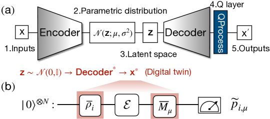
Figure 1: Digital twin-enhanced quantum process tomography. (a) The variational autoencoder (VAE) consists of an encoder and a decoder built with deep neural networks. The input training data x is mapped by the encoder into a parametric probability distribution $\mathcal{N}(\textbf{z};\mu,\sigma^{2})$. The latent variable z is sampled from this distribution and used to reconstruct the output $\textbf{x}^{\prime}$ through the decoder and a pre-designed quantum processing layer (QProcess). (b) The digital twin is applied to reconstruct the error matrix $\textbf{x}^{*}\to\tilde{\chi}^{\rm I}_{\text{err}}$ using a trained VAE, enhancing EM-QPT for a quantum process $\mathcal{E}$.

Error-mitigated QPT. Our objective is to precisely estimate the process matrix of an arbitrary quantum operation $\mathcal{E}$ while accounting for SPAM errors [24, 42, 43, 44]. To suppress these errors, we take the approach outlined in Eq. (7). We utilize identity QPT: only performing state preparation $\mathcal{E}_{\text{sp}}$ and measurement $\mathcal{E}_{\text{m}}$, yielding $\chi^{\text{I}}\equiv\mathcal{E}_{\text{m}}\circ\mathcal{E}_{\text{sp}}$. Ideally, the identity process matrix will be $\chi^{\text{I}}_{mn}=\delta_{m0}\delta_{n0}$, where $\delta_{mn}$ is the Kronecker delta. Deviations from the ideal $\chi^{\text{I}}$ indicate the presence of SPAM errors in the experiment, resulting in $\tilde{\chi}^{I}$, which we refer to as an ‘error matrix’ [43]. By changing argument in the QPT algorithm, we can determine the noisy input states and measurement operators [45]:

$$\mathcal{J}[\{\rho_{i}\},\{M_{\mu}\},\tilde{\chi}^{I}]\rightarrow\{\bar{\rho}_{i}\},\{\bar{M}_{\mu}\}.$$ (8)

When computing $\{\bar{\rho}_{i}\}$, we assume ideal measurement operators, and vice versa (standard quantum state and detector tomography with the error matrix), since gauge symmetry prevents simultaneously determining $\{\bar{\rho}_{i},\bar{M}_{\mu}\}$ with arbitrary accuracy and precision [25, 26, 27, 28].

Here, we benchmark the practical, error-mitigated, and nearly self-consistent version of QPT:

$$\text{EM-QPT}:\mathcal{J}(\bar{\rho}_{i},\bar{M}_{\mu},\tilde{p}_{i,\mu};\tilde{\chi}^{I}).$$ (9)

This approach is resource-intensive, particularly in applications where frequent process characterization is required, such as gate optimization [46, 47]. It is also potentially fragile in the presence of anomaly errors, such as glitches in experiments. Since the error matrix $\tilde{\chi}^{I}$ is independent of the process to be characterized, it is natural to explore whether ML techniques can be leveraged to learn the statistical behavior of SPAM errors hidden in $\tilde{\chi}^{I}$, for more efficient error mitigation.

Inspired by a recent study [40], we use a generative model as a digital twin of the error matrix to enhance EM-QPT. We find that the digital twin, a trained deep neural network, effectively captures the underlying characteristics of SPAM errors, yielding a more refined version of Eq. (8). It can potentially outperform real-time error-matrix acquisition, enabling high-precision QPT with more robust and efficient SPAM-error mitigation.

Variational autoencoder. Our generative model is a variational autoencoder (VAE) [38], which integrates deep learning with probabilistic frameworks to learn a latent representation of training data (see Fig. 1). The VAE consists of an encoder that maps the input x to a latent vector z obeying a probability distribution $\mathbb{Q}(\textbf{z}|\textbf{x})$. The decoder reconstructs the input data $\textbf{x}\to\textbf{x}^{\prime}$ from a sampled latent vector z. To enable backpropagation through the network, the latent variable z is sampled using the reparameterization trick [48]: $\textbf{z}\sim\mathcal{N}(\mu(\textbf{x}),\epsilon\cdot\sigma(\textbf{x}))$, where an auxiliary noise variable is sampled from a normal distribution $\epsilon\sim\mathcal{N}(0,\mathbb{I})$. We use the loss function

$$\textbf{Loss}=\mathcal{L}_{\text{recon}}(\textbf{x}^{\prime},\textbf{x})+\beta D_{\text{KL}}\left[\mathbb{Q}(\textbf{z}|\textbf{x})\parallel\mathcal{N}(\textbf{z}|\textbf{x})\right],$$ (10)

where the mean squared error $\mathcal{L}_{\text{recon}}=\sum_{n,m}(\textbf{x}_{n,m}-\textbf{x}^{\prime}_{n,m})^{2}$ ensures the generated $\textbf{x}^{\prime}$ is similar to x and the Kullback–Leibler (KL) divergence $D_{\text{KL}}$ regularizes $\mathbb{Q}(\textbf{z}|\textbf{x})$ to match a prior normal distribution $\mathcal{N}(\textbf{z}|\textbf{x})$; $\beta$ is a hyperparameter balancing the two losses. Since the learned posterior and the target prior are assumed to be Gaussian distributions, the KL divergence has a closed-form solution [38]: $D_{\text{KL}}\left[\mathbb{Q}(\textbf{z}|\textbf{x})\parallel\mathcal{N}(0,I)\right]=\frac{1}{2}\left(\sigma^{2}+\mu^{2}-1-\log\sigma^{2}\right)$, making it computationally efficient and mathematically well-defined.

Digital twin of the error matrix. We characterize the SPAM errors by constructing the digital twin of the error matrix $\tilde{\chi}^{I}$. First, we collect a training database $\textbf{X}=\{\textbf{x}^{(i)}\}_{i=0}^{N_{x}}$ of $N_{x}$ independent QPT experiments for the identity process, which is implemented by applying a short idle time of a few nanoseconds in experiments. Then we decompose each $\chi$ matrix into two channels of neural networks, corresponding to the real and imaginary parts, forming the input training data points $\chi_{i}\to\textbf{x}^{(i)}\in\mathbb{R}^{2\times d^{2}\times d^{2}}$. To ensure that the VAE output is CPTP, we introduce a QProcess layer [45] using Cholesky decomposition [49, 50]. The digital twin of the error matrix, $\textbf{x}^{\prime}_{i}\to\chi^{\prime}_{i}$, is expected to statistically mimic the major pattern of SPAM errors embedded in the error matrix, enabling ML-enhanced QPT:

ML-QPT $$:\mathcal{J}_{\rm ML}(\bar{\rho}_{i},\bar{M}_{\mu},\tilde{p}_{i,\mu};\chi^{I}_{\text{DT}}),$$

where $\chi^{I}_{\text{DT}}$ is the digital twin of error matrices.

Numerical simulation. In standard $N$-qubit QPT, each qubit is first initialized in an initial state by applying a gate $U_{1}\in\{\texttt{I},\texttt{R}_{x}(-\pi/2),\texttt{R}_{y}(-\pi/2),\texttt{X}\}$. Then, the quantum gate $\mathcal{G}$ under investigation is applied. To enable full process characterization, a set of informationally complete rotation gates $U_{2}\in\{\texttt{I},\texttt{R}_{x}(\pi/2),\texttt{R}_{y}(\pi/2)\}$ are used prior to measuring the qubits in the computational basis. In practice, the noisy readout is composed by

$$\tilde{p}_{i,\mu}=\langle\!\langle M_{\mu}|\mathcal{E}_{\rm m}\circ\mathcal{E}_{\rm gate}(\mathcal{G})\circ\mathcal{E}_{\rm sp}|\rho_{i}\rangle\!\rangle,$$ (11)

where $\mathcal{E}_{\rm m},\mathcal{E}_{\rm gate},\mathcal{E}_{\rm sp}$ represent the error channels acting on the measurement, gate, and initial states, respectively. To simulate incoherent SPAM errors, we use depolarizing error channel $\mathcal{E}_{\rm dep}(\rho;\lambda)=(1-\lambda)\rho+\frac{\lambda}{2^{N}}I$, where $I$ is the identity operator. We randomly sample the error strength for state preparation $\mathcal{E}_{\rm sp}=\mathcal{E}_{\rm dep}(\rho;\lambda_{\rm sp})$ and measurements $\mathcal{E}_{\rm m}=\mathcal{E}_{\rm dep}(\rho;\lambda_{\rm m})$ in terms of a given error rate $\lambda_{1}=\lambda_{\text{m}}+\lambda_{\text{sp}}$ [45]. We also introduce coherent errors with a unitary channel $\mathcal{E}_{\rm uni}(\rho)=U\rho U^{\dagger}$ by adding a rotation shift $\Delta\theta=\theta^{\prime}-\theta_{0}$ on a rotation gate ${\tt R_{i\in[x,y,z]}(\theta_{0})}\to{\tt R_{i\in[x,y,z]}(\theta^{\prime})}$ in SPAM; we uniformly sample the deviation $\Delta\theta/\pi\in[-\lambda_{2},\lambda_{2}]$ ($\lambda_{2}\in[0,1]$). Therefore, we express the total SPAM error as $\lambda_{\text{tot}}=(\lambda_{1}+\lambda_{2})/2\in[0,1]$.

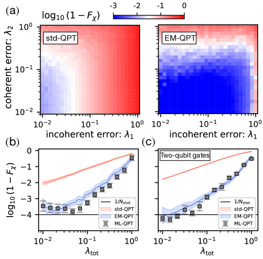
Figure 2: Numerical results for EM-QPT of one- and two-qubit gates. (a) Average process infidelity of single-qubit gates using std-QPT (left panel) and EM-QPT (right panel), as a function of coherent and incoherent errors. (b, c) Fidelity for the evenly mixed error regime for single- and two-qubit gates, respectively. Solid curves and squares are the average results over $10^{2}$ gate samples with shadow and error bar showing one standard deviation. The horizontal line is the statistical error $1/N_{\text{shot}}$ with the shot number $N_{\text{shot}}=10^{4}$.

The numerical experiment consists of three steps: (i) set $\mathcal{G}={\tt I}$, the $N$-qubit identity gate, and perform std-QPT to obtain the error matrix $\tilde{\chi}^{I}$; (ii) reconstruct $4^{N}$ noisy quantum states and $6^{N}$ observables using Eq. (8); (iii) perform std-QPT on a randomly selected unitary gate $\mathcal{G}$ using the error-mitigated probes, giving a corrected process matrix $\tilde{\chi}^{3}_{e}$ according to Eq. (7). Here, we focus on unitary operations, but the EM-QPT approach is valid for general CPTP processes [45].

In Fig. 2, we present numerical results for std-QPT, EM-QPT, and ML-QPT under the influence of both incoherent and coherent errors. Each data point represents the average process infidelity [51] computed over $10^{2}$ randomly chosen unitary gates. Particularly, in Fig. 2(a), we analyze the gate infidelity as a function of coherent error $\lambda_{2}$ and incoherent error $\lambda_{1}$ for a single-qubit system. Furthermore, we investigate how the infidelity scales with the total error $\lambda_{\rm tot}$ in the case of evenly mixed contributions, i.e., $\lambda_{1}=\lambda_{2}$, with the corresponding results for one- and two-qubit gates presented in Fig. 2(b) and 2(c), respectively. For ML-QPT, we collected $10^{3}$ error matrices of each data point to train a digital twin model across a range of $\lambda_{\text{tot}}$, and achieved better performance than with EM-QPT, as seen in Fig. 2(b)-(c).

Experiments on single-qubit Clifford gates. Next, we verify EM-QPT in experiments with single-qubit Clifford gates. We consider the average gate fidelity [52, 53, 54]

$$\mathcal{F}_{\text{gate}}=\frac{d\mathcal{F}_{\chi}+1}{d+1},$$ (12)

where $d=2^{N}$ is the Hilbert-space dimension of the $N$-qubit system; the process fidelity $\mathcal{F}_{\chi}$ [51] is obtained through QPT. For small errors ($\lambda_{\text{tot}}\to 0$) randomized benchmarking (RB) [55] statistically captures the average gate error over Clifford gates, implying that the RB fidelity then approximates the average gate fidelity: $\mathcal{F}_{\text{rb}}\approx\mathcal{F}_{\text{gate}}$.

We implement our method on 24 single-qubit Clifford gates on a superconducting quantum processor (see Device A  [45, 56]). Coherent errors are introduced by adding rotation uncertainties to the single-qubit gates through amplitude fluctuations in the cosine-shaped DRAG pulses [57]: the target amplitude $A_{0}$ is modified to $A^{\prime}=(1+\delta)A_{0}$, with the offset $\delta$ uniformly sampled as $\delta\sim\mathcal{U}(-\lambda_{2},\lambda_{2})$ ($\lambda_{2}\in[0,1]$). Incoherent errors are introduced by biasing the amplitude of reset and readout pulses by $\lambda_{1}$ [scaling the optimized pulse by $(1-\lambda_{1})$]. See Appendix C in Ref. [45] for details about the error setup.

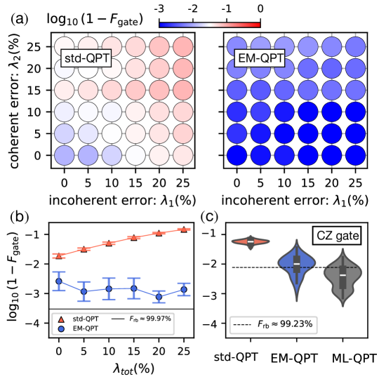
Figure 3: Experimental results for one- and two-qubit gates. (a) Performance of std-QPT (left) and EM-QPT (right) as a function of coherent and incoherent errors. (b) The points from (a) while $\lambda_{1}=\lambda_{2}$. Each data point in (a)/(b) is averaged over $15$/$10^{2}$ QPT experiments for all 24 single-qubit Clifford gates. (c) Infidelity distribution over $10^{2}$ QPT experiments of a CZ gate estimated with std-QPT, EM-QPT, and ML-QPT. Here, SPAM errors $\sim$6\text{\,}\mathrm{\char 37\relax}$$ and the RB fidelity is $99.23\text{\,}\mathrm{\char 37\relax}$.

In Fig. 3(a)-(b), we present experimental results for std-QPT and EM-QPT for single-qubit Clifford gates under varying levels of coherent and incoherent SPAM errors; EM-QPT yields at least an order-of-magnitude improvement in gate fidelity. Notably, RB outperforms EM-QPT because SP and M errors cannot be explicitly separated from the error matrix. We leave further optimization of the QPT method [24] through adjusting the weight function between SP and M for future work.

Experiments on two-qubit CZ gates. We start with a well-tuned adiabatic ${CZ}$ gate with $\mathcal{F}^{CZ}_{\text{rb}}\sim$99.23\text{\,}\mathrm{\char 37\relax}$$ (see Device B  [45, 58]). We perform identity QPT followed by QPT of this gate $10^{2}$ times. We can thus obtain the process fidelity of the CZ gate with both EM-QPT and ML-QPT. In Fig. 3(c), we present the probability distribution of gate infidelity estimated by Eq. (12) using std-QPT, EM-QPT, and ML-QPT; the ML-QPT results are based on a digital twin trained on the $10^{2}$ error matrices.

Precision and sensitivity. The gate fidelity of an unknown gate $G$ can be statistically estimated over the set $\mathcal{S}_{I}=\{\tilde{\chi}^{I}_{1},\tilde{\chi}^{I}_{2},...,\tilde{\chi}^{I}_{N_{\text{err}}}\}$, forming a probability distribution $\mathbb{P}_{\text{EM}}(\mathcal{F}(G;\tilde{\chi}^{I}))|_{\tilde{\chi}^{I}\in\mathcal{S}_{I}}$, where the variance is primarily induced by SPAM errors. However, averaging fidelity over all error matrices may reduce EM-QPT precision due to experimental anomalies. To address this, we use ML to extract the dominant SPAM error patterns, creating a digital twin that reconstructs them. Therefore, the gate fidelity relying on the digital twin admits the distribution $\mathbb{P}_{\text{ML}}(\mathcal{F})|_{{\tt D^{*}(\textbf{z})}\to\chi^{I}}$, where ${\tt D^{*}}(\textbf{z})|_{\textbf{z}\sim\mathcal{N}(0,\mathbb{I})}$ is the decoder from the trained VAE model.

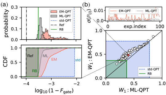
Figure 4: Precision and sensitivity. (a) Top: infidelity distribution of EM-QPT and ML-QPT, based on the training dataset and digital twin, compared with std-QPT (dashed blue), reference (dot-dashed black), and RB (solid green). Bottom: CDFs used to calculate the $W_{1}$ distance from the reference distribution. (b) Top: standard deviations $\sigma(\mathbb{P}_{(i)})$ of the fidelity distributions based on EM-QPT and ML-QPT for a testing dataset comprising $10^{2}$ QPT experiments on X gates. Bottom: normalized $W_{1}$ distance of EM-/ML-QPT. The blue and green shaded regions indicate cases where the $W_{1}$ distance is smaller than that of std-QPT and RB, respectively. Parameters: $\xi_{\rm max}=5,\xi_{\rm min}=1,\xi_{0}=4$.

We next evaluate the performance of our method through empirical information theory [59, 60], which focuses on the behavior of information measures in practical, finite-sample settings. To quantify the precision and sensitivity of gate characterization, we calculate the distance between the empirical $\mathbb{P}_{(i)}(q)$ and reference $\mathbb{P}_{\rm ref}(q)$ probability distributions by the one-dimensional Wasserstein (earth mover’s) distance [61]

$$W_{1}(\mathbb{P}_{(i)},\mathbb{P}_{\rm ref})=\int_{\mathbb{R}}|\mathcal{C}_{(i)}(q)-\mathcal{C}_{\rm ref}(q)|dq,$$ (13)

where $\mathcal{C}_{P}(q^{\prime})=\text{Prob}[q\leq q^{\prime}]$ is the cumulative distribution function (CDF) of the probability distribution $P$. The $W_{1}$ distance is the area between the CDF curve $P$ and the reference; see the lower panel in Fig. 4(a). This distance directly captures first-moment deviations and provides an informative proxy for the second moment.

We take the basis $q=\log_{10}(1-\mathcal{F})\in[-\xi_{\rm max},-\xi_{\rm min}]$ with constants $\xi_{{\rm max}/{\rm min}}\in\mathbb{R}^{+}$. For simplicity, we set the reference probability distribution as a delta function $\mathbb{P}_{\rm ref}=\delta(-\xi_{0})$ referring to the ideal measurement protocol that always perfectly estimates the gate fidelity $\mathcal{F}_{0}=1-10^{-\xi_{0}}$ fulfilling $\xi_{0}\in[\xi_{\rm min},\xi_{\rm max}]$. The $W_{1}$ distance then obeys $W_{1}\in[0,\xi_{\rm max}-\xi_{\rm min}]$, where $W_{1}=0$ is the ideal measurement scheme that gives the exact gate fidelity. The larger the $W_{1}$ distance, the further away from the perfect characterization.

In Fig. 4(a)-(b), we compare the normalized $W_{1}/(\xi_{\rm max}-\xi_{\rm min})$ distance of the EM-QPT and ML-QPT methods for $10^{2}$ QPT experiments of an X gate, using $10^{3}$ realistic error matrices and their corresponding digital twin, respectively. We take the distribution of std-QPT and RB as delta functions, since the uncertainty for an individual QPT is negligible. In Fig. 4(a), the probability distribution of EM-QPT (pink) contains all types of errors in error matrices, implying large variance in fidelity estimation in due to abnormal errors. Consequently, ML-QPT yields more reliable fidelity estimates, leading to a smaller $W_{1}$ distance than EM-QPT in Fig. 4(b).

Discussion and conclusion. We have proposed nearly self-consistent and SPAM-error-mitigated quantum process tomography (EM-QPT) by constructing noisy probes from identity process matrices. Moreover, we introduced machine-learning-assisted QPT (ML-QPT), further enhancing EM-QPT by fully leveraging knowledge of SPAM errors hidden in identity process matrices, enabling accurate and high precision QPT for reliable and practical applications across a variety of quantum devices. The SPAM-aware digital twin improves gate characterization beyond standard methods, allowing accurate fidelity estimation up to the second moment. Both numerical simulations and experimental results demonstrate that our method achieves at least an order-of-magnitude improvement in precision over standard QPT.

A possible extension of our method is to diagnose the type of SPAM error; for example, the particular behavior of coherent and incoherent errors, providing a useful reference for experimental design. The digital twin of SPAM errors can also serve as a sensitive sensor to detect anomalies in realistic experiments [40]. More broadly, our approach can be directly extended to $N$-qubit ($N>2$) quantum processes [8, 62], providing an efficient toolkit in quantum technology, e.g., for gate optimization [46, 47]. Furthermore, our EM-QPT (ML-QPT) protocol has great potential in ancilla-assisted QPT, where input states are often entangled and the measurement schemes involve intricate global measurements with complex unitary operations [63, 64].

Code availability. The codes that support the findings of this study are openly available in the repository https://github.com/huangtangy/EM-QPT.

Supplemental Material of
“Quantum Process Tomography with Digital Twins of Error Matrices"

For simplicity and clarity in our derivations, we use the Pauli-Liouville representation as a framework. The Pauli set reads

$$\mathcal{P}:=\left\{\bigotimes_{v=1}^{N}E_{v}:E_{v}\in\{I,\sigma_{x},\sigma_{y},\sigma_{z}\}\right\},$$ (14)

where $I$ is the identity matrix, and $\sigma_{x},\sigma_{y}$, and $\sigma_{z}$ are the standard Pauli matrices. In this framework, the density matrix $\rho$ and a quantum channel $\mathcal{E}(\rho)$ can be expressed as

$$\rho=\sum_{j=1}^{4^{N}}a_{j}E_{j},\quad\mathcal{E}(\rho)=\sum^{4^{N}}_{\alpha,\beta=1}\chi_{\alpha\beta}E_{\alpha}\rho_{0}E_{\beta}^{\dagger},$$ (15)

where $E_{j}\in\mathcal{P}$ and $a_{j}=\text{Tr}(E_{j}^{\dagger}\rho)/{2^{N}}$. To facilitate further analysis, we vectorize the density operator:

$$\text{vec}(\rho)=|\rho\rangle\!\rangle=(\rho_{1},\rho_{2},\dots,\rho_{4^{n}})^{T},\quad\mathcal{E}(\rho)=\chi\circ|\rho\rangle\!\rangle.$$ (16)

Here, the symbol $A\circ B$ denotes the completely positive trace-preserving (CPTP) mapping of $A$ acting on $B$. Additionally, we note the trace property

$$\text{Tr}[\hat{O}\rho]=\text{vec}(\hat{O}^{T})|\rho\rangle\!\rangle=\langle\!\langle\hat{O}|\rho\rangle\!\rangle.$$ (17)

.1 Appendix A: Estimation of noisy probes

The objective of this section is to estimate the noisy probes, including both quantum states and measurements, based on the process tomography of the idling process. Specifically, we aim to perform state and detector tomography by leveraging the error matrix.

To achieve this, we define a loss function that incorporates the state $\rho$, measurement $M$, and process matrix $\chi$:

$$\mathcal{J}(M,\rho,\chi)=\big{\|}\textbf{A}|\chi\rangle\!\rangle-\langle\!\langle M|\rho\rangle\!\rangle\big{\|},$$ (18)

where $\parallel\cdot\parallel$ represents the $L_{2}$ norm and A is the sensing matrix, which can be computed analytically [21]. The loss function in Eq. (18) quantifies the discrepancy between the ideal readout and the experimental outcomes obtained for given initial states and measurement setups.

Given the process matrix $\tilde{\chi}^{I}$ obtained from identity process tomography, the noisy initial states can be estimated by solving the optimization problem

$$\overline{\rho}_{i}={\operatorname*{argmin}_{\rho_{i}}}\sum_{\mu}\mathcal{J}(\rho_{i},M_{\mu},\tilde{\chi}^{I})$$

subject to $$\quad\text{Tr}(\rho_{i})=1,\quad\rho_{i}^{\dagger}=\rho_{i},\quad\rho_{i}\geq 0.$$ (19)

Here, we assume that the measurement probes $\{M_{\mu}\}$ are perfect, and the optimized states satisfy the trace condition $\text{Tr}(\rho_{i})=1$, Hermiticity ($\rho^{\dagger}=\rho_{i}$), and positive semi-definiteness ($\rho_{i}\geq 0$).

Similarly, the noisy measurement probes can be estimated by

$$\{\overline{M}_{\mu}\}=\operatorname*{argmin}_{\{{M}_{\mu}\}}\sum_{i}\mathcal{J}(\rho_{i},\{{M}_{\mu}\},\tilde{\chi}^{I})$$

$$\quad\text{subject to}\quad\sum_{\mu}M_{\mu}=\mathbb{I},\quad M_{\mu}\geq 0,$$ (20)

where the initial states are assumed to be perfect, and the estimated positive operator-valued measures (POVMs) satisfy the properties of positivity and completeness. These optimizations are performed using the Python-based library cvxpy [41].

.2 Appendix B: EM-QPT on an arbitrary $N$-qubit quantum channel

In this section, we investigate the performance of our method for a general CPTP quantum channel, which can be expressed in the Pauli basis. The Kraus operators $\{\mathcal{K}^{(i)}\}$ can be expressed in the Pauli basis $\{E_{k}\}$ [Eq. (14)] as

$$\mathcal{K}^{(i)}=\sum_{k}^{4^{N}}c^{(i)}_{k}E_{k},$$ (21)

where $c_{k}^{(i)}\in\mathbb{C}$ are complex coefficients. For an $N$-qubit system, any CPTP map can be constructed using up to $r\leq 4^{N}$ Kraus operators:

$$\mathcal{E}_{\text{rand}}(\rho)=\sum^{r\leq 4^{N}}_{i=1}\mathcal{K}^{(i)}\rho(\mathcal{K}^{(i)})^{\dagger},$$ (22)

with the trace-preserving condition requiring $\sum_{i=1}^{r}(\mathcal{K}^{(i)})^{\dagger}\mathcal{K}^{(i)}=\mathbb{I}$.

To numerically generate valid CPTP maps, we first sample random complex coefficients $\{c_{k}^{(i)}\}\in\mathbb{C}^{4^{N}\times r}$ to form unnormalized Kraus operators $\{\mathcal{K^{\prime}}^{(i)}=\sum_{k}c_{k}^{(i)}E_{k}\}_{i=1}^{r}$, and then normalize them to satisfy the TP condition:

$$\mathcal{K}^{(i)}=\frac{\mathcal{K^{\prime}}^{(i)}}{\sqrt{\sum^{r}_{i=1}\mathcal{K^{\prime}}^{(i)}(\mathcal{K^{\prime}}^{(i)})^{\dagger}}}.$$ (23)

The resulting process matrix $\chi$, defined through

$$\chi_{\alpha\beta}=\sum_{i}c^{(i)}_{\alpha}(c^{(i)}_{\beta})^{*},$$ (24)

is guaranteed to be Hermitian and completely positive by construction.

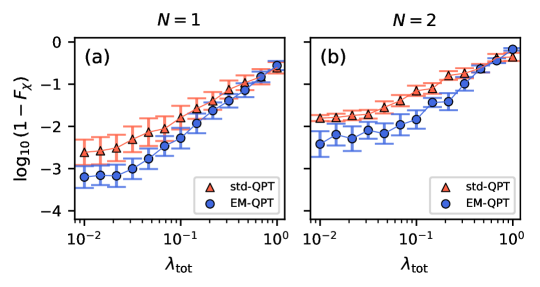
Figure 5: EM-QPT of general CPTP processes for one- and two-qubit quantum process. Process infidelity as a function of total SPAM error for (a) single- and (b) two-qubit CPTP processes with randomly sampled Kraus number. The orange triangles and blue circles are the results averaged over $10^{2}$ random CPTP processes with an error bar of one standard deviation.

We insert the quantum operation $\mathcal{E}_{\text{rand}}(\cdot)$ in the quantum circuit by using the function ${\tt Kraus}(\{\mathcal{K}^{(i)}\})$ in ${\tt qiskit}$ platform. To investigate the EM-QPT for a general CPTP process, we randomly sample the Kraus number $r\in[1,4^{N}]$ for $N$-qubit quantum channel. The process fidelity as a function of total SPAM error are presented in Fig. 5 for one- and two-qubit channels, respectively.

.3 Appendix C: Digital twinning of the error matrix

.3.1 1. The generative model: variational autoencoder

A variational autoencoder (VAE) [38] is a generative model that combines deep learning with probabilistic frameworks to learn a latent representation of data. Unlike traditional autoencoders [66], a VAE models the latent space as a probability distribution rather than fixed embeddings. Specifically, a VAE consists of an encoder that maps the input x to a latent distribution $\mathbb{Q}(\textbf{z}|\textbf{x})\sim\mathcal{N}(\mu,\sigma^{2})$, where $\mu$ and $\sigma^{2}$ are learned through separate fully connected layers. The decoder reconstructs the input data $\textbf{x}^{\prime}$ from a sampled latent vector z.

To enable backpropagation through the network, the latent variable z is sampled using the reparameterization trick [48]:

$$\textbf{z}=\mu(\textbf{x})+\epsilon\cdot\sigma(\textbf{x}),$$ (25)

where $\epsilon\sim\mathcal{N}(0,1)$ is an auxiliary noise variable sampled from a standard normal distribution. The total loss function of the VAE consists of two components:

$$\textbf{Loss}=\mathcal{L}_{\text{recon}}(\textbf{x}^{\prime},\textbf{x})+\beta D_{\text{KL}}\left[\mathbb{Q}(\textbf{z}|\textbf{x})\parallel\mathbb{P}(\textbf{z})\right],$$ (26)

where the reconstruction loss $\mathcal{L}_{\text{recon}}=\sum_{n,m}(\textbf{x}_{n,m}-\textbf{x}^{\prime}_{n,m})^{2}$ ensures that the reconstructed data $\textbf{x}^{\prime}$ closely matches the original input x, and the Kullback–Leibler (KL) divergence $D_{\text{KL}}$ regularizes the learned posterior $\mathbb{Q}(\textbf{z}|\textbf{x})$ to match the prior $\mathbb{P}(\textbf{z})=\mathcal{N}(0,\mathbb{I})$. The hyperparameter $\beta$ balances the two loss terms. Since both the learned posterior and the target prior are Gaussian distributions, the KL divergence has a closed-form solution [38]:

$$D_{\text{KL}}\left[\mathbb{Q}(\textbf{z}|\textbf{x})\parallel\mathcal{N}(0,I)\right]=\frac{1}{2}\left(\sigma^{2}+\mu^{2}-1-\log\sigma^{2}\right).$$ (27)

.3.2 2. Unsupervised learning of error matrices

The goal of this section is to learn the state preparation and measurement (SPAM) errors by training a generative model on realistic experimental data. We hypothesize that a deep neural network (NN)-based model can statistically generate the idle process matrix, capturing the features of SPAM errors. This NN serves as a digital twin [40] of the SPAM error.

To achieve this, we first construct a training database $\textbf{X}=\{\textbf{x}^{(i)}\}_{i=0}^{N_{x}}$, consisting of $N_{x}$ independent quantum process tomography (QPT) experiments for the idling quantum process. For an $N$-qubit quantum channel, the error matrix is a complex matrix $\chi_{i}\in\mathbb{C}^{4^{N}\times 4^{N}}$. Each $\chi$ matrix is decomposed into real and imaginary parts, forming the input training data points $\textbf{x}_{i}\in\mathbb{R}^{2\times 4^{N}\times 4^{N}}$.

In this framework, the digital twin of the error matrix, $\textbf{x}^{\prime}_{i}\to\chi^{\prime}_{i}$, is expected to statistically mitigate SPAM errors for an arbitrary quantum process $\mathcal{E}$. The neural network learns the underlying features of SPAM errors embedded in the error matrix, enabling enhanced QPT with the assistance of the digital twin.

The encoder extracts key features from the input data $\textbf{x}_{i}$ using a series of convolutional layers [66], progressively reducing the spatial dimensions while increasing the number of channels. At the end of this process, the high-dimensional input is transformed into a low-dimensional feature representation. Instead of encoding the input into a fixed lower-dimensional representation $\textbf{x}\to\textbf{z}$, the VAE learns a probabilistic distribution characterized by two variational parameters $\{\mu,\sigma^{2}\}$, such that $\textbf{z}\sim\mathcal{N}(\mu,\sigma^{2})$.

To ensure that the VAE output satisfies the CPTP constraint, we introduce an additional layer called QProcess, which relies on the Cholesky decomposition [49]$:\mathbf{B}=\mathbf{L}\mathbf{L}^{T}$, where $\mathbf{L}$ is a lower triangular matrix and $\mathbf{L}^{T}$ is its transpose. Cholesky decomposition is a powerful mathematical tool that plays a significant role in quantum information science, both in QPT [50] and quantum state tomography (QST) [67]. To ensure numerical stability, the transformed output is $\mathbf{x}=\mathbf{L}\mathbf{L}^{T}+\epsilon\mathbf{I}$, where $\epsilon$ is a small positive number (e.g., $10^{-5}$).

As a result, the forward data flow of the model is

$$\textbf{x}\to\tt{Encoder}\to\textbf{z}\to\tt{Decoder}\to\tt{QProcess}\to\textbf{x}^{\prime}.$$ (28)

For a well-trained model (denoted ^∗), there is a straightforward approach to evaluating the VAE model. As mentioned earlier, the goal of VAE is to map the training data set to a Gaussian distribution that closely approximates the standard normal distribution. In this context, one can verify the distribution of the latent vectors by passing the training data through the trained encoder as

$$\textbf{x}\to\tt{Encoder}^{*}\to\textbf{z}^{\prime},$$ (29)

where, ideally, $\textbf{z}^{\prime}\sim\mathcal{N}(0,\mathbb{I})$.

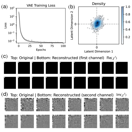
Figure 6: Training outcomes of the VAE model for generating digital twins of two-qubit error matrices. (a) Evolution of the training loss over 100 epochs, showing a rapid initial decrease and eventual convergence, indicating successful training. (b) Distribution of the latent vectors $\mathbf{z}^{\prime}$ obtained by encoding the training dataset using the trained encoder. The probability density function (PDF) is estimated via Gaussian kernel density estimation (blue curves), demonstrating that the learned latent representation closely follows a standard normal distribution. (c) Comparison between original (top) and reconstructed (bottom) error matrices for the real component (first channel) of the two-qubit gate errors. The reconstructed matrices are generated by decoding latent vectors sampled from the trained encoder. (d) Similar comparison for the imaginary component (second channel) of the error matrices. The results indicate that the VAE successfully captures the statistical properties of the error matrices, enabling the generation of realistic digital twins for quantum process tomography and error mitigation. The total error rate is $\lambda_{\text{tot}}=0.01$ and the size of traning data sets is $10^{3}$.

In Fig. 6(a)-(b), we illustrate the evolution of the loss during training and the distribution of the latent vectors $\textbf{z}^{\prime}$ across the entire training dataset. The probability density function (PDF) of $\textbf{z}^{\prime}$ is estimated using Gaussian kernel density estimation [68] and is depicted by the blue curves in Fig. 6(b). The results indicate that the two-dimensional latent vectors $\textbf{z}^{\prime}$ produced by the trained encoder are close to a standard normal distribution.

Following this, digital twins can be automatically generated by sampling the latent space from a normal distribution:

$$\textbf{z}\sim\mathcal{N}(0,\mathbb{I})\to\tt{Decoder}^{*}\to\tt{QProcess}^{*}\to\textbf{x}^{*},$$ (30)

where $\textbf{x}^{*}$ denotes the digital twin of error matrices. We now present the VAE-generated digital twin of error matrices for two-qubit unitary gates with an error rate of $\lambda_{\text{tot}}=0.01$. In Fig. 6(c)-(d), we compare the reconstructed data for the real (first channel) and imaginary components (second channel) of the error matrices with those sampled from the training dataset.

This approach enables the generation of error matrices that statistically capture the characteristics of SPAM errors, providing an efficient tool for constructing the error-mitigated quantum process tomography.

The whole training process is performed using the PyTorch [69] framework.

.4 Appendix D: Experimental details

In this section, we detail the devices, experimental setup, and QPT protocol together with our implementation of the noise channels.

Parameter		Value
Qubit frequency,	$\omega_{0}/2\pi$	$3.772\text{\,}\mathrm{GHz}$
Qubit anharmonicity,	$\alpha_{0}/2\pi$	$-222\text{\,}\mathrm{MHz}$
Resonator frequency,	$\omega_{r}/2\pi$	$6.439\text{\,}\mathrm{GHz}$
Dispersive shift,	$\chi_{r}/2\pi$	$0.350\text{\,}\mathrm{MHz}$
Relaxation time,	$T_{1}$	$131\text{\,}\mathrm{\SIUnitSymbolMicro s}$
Decoherence time,	$T_{2}^{*}$	$64\text{\,}\mathrm{\SIUnitSymbolMicro s}$
Spin Echo,	$T_{2}^{Echo}$	$141\text{\,}\mathrm{\SIUnitSymbolMicro s}$
Single-qubit gate fidelity,	$F_{1Q}$	$99.963\text{\,}\mathrm{\char 37\relax}$
Two-state assignment fidelity,	$F_{\text{Assign}(|0\rangle,|1\rangle)}$	$95.65\text{\,}\mathrm{\char 37\relax}$

Table 1: Device A. Measured qubit parameters, coherence properties, and single-qubit performance.

.4.1 1. Device details

The parameters of the sample (Device A) used in the experiment with single-qubit gate are listed in Table 1. The sample qubit is a subsystem of a device comprising two fixed-frequency xmon-style transmon qubits [70] capacitively coupled via a frequency-tunable anharmonic oscillator. The sample used in this work is the same as the quantum processor studied in Ref. [56]. Device schematic and micrograph presented in Fig. 7. The two qubits are capacitively coupled to individual control lines and quarter-wavelength resonators for readout. The tunability of the coupler is provided by two Josephson junctions in a superconducting quantum interference device (SQUID) configuration. Our experiments were performed at the zero-flux sweet spot, where the coupler had the maximal frequency, to suppress the interaction with the qubit under investigation.

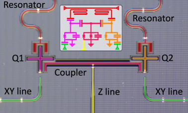
Figure 7: Single-qubit gate device micrograph with false colors. The device used for single-qubit gate experiment consists of two fixed-frequency xmon-style transmon qubits coupled via a frequency-tunable anharmonic oscillator with SQUID. The insertion shows the circuit schematic. Only the left qubit (Q1) is used for the experiment.

To implement the two-qubit CZ gate, we used a device (Device B) with two fixed frequency transmons (Q1 and Q2) coupled via flux-tunable coupler as shown in Fig. 8. The device parameters are given in Table 2. We executed the gate using baseband pulses on the coupler leading to adiabatically acquiring $\pi$ phase on the target qubit when control qubit is in excited state.

Figure 8: Two-qubit gate device micrograph with false coloring. The device used for two qubit gate consists of two fixed-frequency transmons and one flux tunable coupler. The right-hand side image shows a zoomed-in view of the Z-line (yellow), shorted to ground, inductively coupled to the SQUID loop of the coupler.

Parameter	Q1	Q2
Qubit frequency ($\omega_{0}/2\pi$)	$4.7744\text{\,}\mathrm{GHz}$	$4.6841\text{\,}\mathrm{GHz}$
Qubit anharmonicity ($\alpha_{0}/2\pi$)	$-239\text{\,}\mathrm{MHz}$	$-239\text{\,}\mathrm{MHz}$
Resonator frequency ($\omega_{r}/2\pi$)	$6.997\text{\,}\mathrm{GHz}$	$6.852\text{\,}\mathrm{GHz}$
Dispersive shift ($\chi_{r}/2\pi$)	$0.420\text{\,}\mathrm{MHz}$	$0.390\text{\,}\mathrm{MHz}$
Relaxation time ($T_{1}$)	$66\text{\,}\mathrm{\SIUnitSymbolMicro s}$	$84\text{\,}\mathrm{\SIUnitSymbolMicro s}$
Decoherence time ($T_{2}^{*}$)	$45\text{\,}\mathrm{\SIUnitSymbolMicro s}$	$57\text{\,}\mathrm{\SIUnitSymbolMicro s}$
Single-qubit gate fidelity ($F_{1Q}$)	$99.948\text{\,}\mathrm{\char 37\relax}$	$99.966\text{\,}\mathrm{\char 37\relax}$
Three-state assignment fidelity ($F_{\text{Assign}(|0\rangle,|1\rangle,|2\rangle)}$)	$93\text{\,}\mathrm{\char 37\relax}$	$94.3\text{\,}\mathrm{\char 37\relax}$

Table 2: Device B. Measured qubit parameters, coherence properties, and gate performances for experiments on a two-qubit gate device.

.4.2 2. Experimental setups

Experiments with single-qubit gates were conducted in a Bluefors XLD400 dilution refrigerator maintaining a base temperature stabilized at $\sim$15\text{\,}\mathrm{mK}$$. The room-temperature setup, together with the full wiring diagram in our dilution refrigerator, is the same as in Ref. [56]. The drive pulses for the qubits and resonators are generated by a combination of Quantum Machines Operator-X (OPX+) quantum controller and Quantum Machines Octave. The IF (intermediate frequency) signals from the OPX+’s arbitrary-waveform generators are fed to the built-in IQ mixers of the Octave and combined with signals from the internal local oscillators. Then the outputs of the Octave are fed into qubit drive lines, which are capacitively coupled to the transmon circuits, or into the readout feedline capacitively coupled to the resonators on chip.

The transmitted readout signal propagates through the sample to a double junction circulator (48 from Low Noise Factory), a directional coupler (412), and a traveling wave parametric amplifier (TWPA) fabricated at VTT Technical Research Center of Finland. After TWPA amplification the signal transmits through a single junction circulator (48 GHz from QuinStar Technology), a series of low-pass, infrared, and high-pass filters, as well as an additional double junction circulator (48 GHz from Low Noise Factory), before being amplified by around $40\text{\,}\mathrm{dB}$ at $4\text{\,}\mathrm{K}$ with a high-electron-mobility transistor (HEMT) from Low Noise Factory. In addition, the room-temperature microwave amplifier from Narda-MITEQ is connected to the readout chain outside of the dilution refrigerator. The pump signal and the DC bias current for the TWPA are provided by an Anritsu MG3692 signal generator and Yokogawa GS200, through a current limiting resistor. Circulators in the output line are essential to prevent strong signals from reflecting back into the sample. Finally, the output signal is down-converted inside the Octave to the hundreds of MHz range to be recorded and integrated by the OPX+ internal digitizer.

The schematic diagram of the measurement setup for the two-qubit gate experiment is the same as in Ref. [58]. The device is mounted at the $10\text{\,}\mathrm{mK}$ stage of a Bluefors LD250 dilution refrigerator. The drive pulses for the qubits and resonators are generated by a QBLOX cluster, which consists of QCM-RF, QRM-RF, and QCMmodules. QCM-RF controls the single-qubit gates via the XY drive lines (see Fig. 8). Multiplexed readout is performed with QRM-RF. Flux pulses to the coupler are applied to the Z line (see Fig. 8) from the QCM control module that can send arbitrary pulses from DC to $400\text{\,}\mathrm{MHz}$.

.4.3 3. Gate calibration

Calibrations of the fundamental transition frequencies and coherence times provided in Table 1 mainly follow well-established parameter-estimation methods used for superconducting quantum computing [71]. Once the qubit frequency and coherence times are determined, we calibrate the amplitudes of $\pi/2$ ($\pm\text{X90}$ and $\pm\text{Y90}$) and $\pi$-pulses (X180 and Y180) for later use in standard quantum process tomography (std-QPT) and randomized benchmarking (RB). Our single-qubit pulses use a cosine envelope with a $40\text{\,}\mathrm{ns}$ duration, combined with the derivative removal by adiabatic gate (DRAG) [57] technique.

The goal of the calibration is to determine the correct amplitudes of the $\pi/2$ and $\pi$ pulses, and then the corresponding DRAG coefficients. Amplitude tune up is performed via repeatedly executing pseudo-identity pulse sequences (such as two $\pi$-pulses or four $\pi/2$-pulses) $N$ times and measuring the state of the qubit across different pulse amplitudes and number of pulses. For the DRAG calibration we utilized the “Google method” [72]. Both protocols are implemented on the Quantum Machines OPX+ and Octave based on open-source libraries for pulse-level control of quantum bits built with the QUA programming language. The programming code is similar to the example described in Ref. [73].

.4.4 4. Interleaved randomized benchmarking

The performance of the single-qubit gates is characterized with Clifford RB [55]. To implement this technique, we generate random sequences of single-qubit Clifford gates from Table 3 and measure the state of the qubit afterwards. Each random sequence ends with the recovery gate that will bring the qubit back to its ground state. It should be noted here that the average number of single-qubit gates in Clifford operation is 1.875.

Index	Combinations
1	[I]
2	[X180]
3	[Y180]
4	[Y180, X180]
5	[X90, Y90]
6	[X90, -Y90]
7	[-X90, Y90]
8	[-X90, -Y90]
9	[Y90, X90]
10	[Y90, -X90]
11	[-Y90, X90]
12	[-Y90, -X90]
13	[X90]
14	[-X90]
15	[Y90]
16	[-Y90]
17	[-X90, Y90, X90]
18	[-X90, -Y90, X90]
19	[X180, Y90]
20	[X180, -Y90]
21	[Y180, X90]
22	[Y180, -X90]
23	[X90, Y90, X90]
24	[-X90, Y90, -X90]

Table 3: Single-qubit Clifford gates.

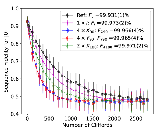
Figure 9: Interleaved randomized benchmarking (RB) of single-qubit gates. All curves are averaged over 50 random seeds.

In the case of the interleaved RB, we are aiming to characterize the fidelity of a specific gate. Here, we use the gate of interest (I, X90, Y90, X180) to construct the pseudo-identity gate (implemented as a $40\text{\,}\mathrm{ns}$ delay, four X90 gates, four Y90 gates, or two X180 gates, respectively) which is interleaved between each Clifford gate in the random sequence. Experimental results are shown in Fig. 9. For each circuit depth, measurements are performed for a large number (50) of different random sequences. It is clearly seen that the average gate fidelity exceeds $99.96\text{\,}\mathrm{\char 37\relax}$.

.4.5 5. QPT protocol and noise channels

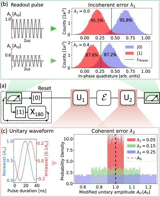
Figure 10: Schematic diagram of QPT and implementation of noise channels. (a) Quantum process tomography with active reset (dashed rectangle) for the initialization of the qubit in the ground state $|0\rangle$. $U_{1}$ and $U_{2}$ are the sets of unitary rotations responsible for initial state preparation and measurement projectors, respectively. $\mathcal{E}$ is the process under study. (b) Incoherent noise channel, where the amplitude of the readout pulse (left graph) as well as $I_{\text{Thresh}}$ (vertical green line in the right graph) are scaled by a factor of $(1-\lambda_{1})$. Readout signal histograms visualize the separation between the peaks from the ground $|0\rangle$ (blue) and excited $|1\rangle$ (red) states for different $\lambda_{1}$ values. The state-assignment fidelities are written on top of the corresponding histograms. (c) Coherent noise channel, where the amplitude $A_{U}$ of the unitary waveforms (left graph) are modified according to $A_{U}=A_{0}[1+r\cdot\lambda_{2}]$, where $r\sim\mathcal{U}(-1.0,\ 1.0)$ is a uniformly distributed random number. Probability density (right graph) of the modified unitary amplitude for different coherent errors $\lambda_{2}$. In the experiment, for each value of $\lambda_{2}$, the amplitude is sampled 10,000 times to obtain the corresponding distribution.

In our experiments, we performed std-QPT as shown in Fig. 10(a) with minor modifications allowing us to introduce different noise channels as desired. We detail the QPT protocol below.

1. Active reset. Each experiment begins with an active reset procedure to initialize the qubit in the ground state $|0\rangle$. Here, we start by measuring the qubit state with a readout pulse of $2\text{\,}\mathrm{\SIUnitSymbolMicro s}$. After digitization, the state is encoded in the in-phase component according to an initial calibration similar to Ref. [74], where we optimize the information obtained from the readout signal by deriving the optimal integration weights. The aim is to maximize the separation of the IQ blobs when the ground and excited state are measured. In a one-dimensional (1D) histogram, shown in the top right of Fig. 10(b), we can see that the peaks from the ground $|0\rangle$ (blue) and excited $|1\rangle$ (red) states are separated from each other along the in-phase quadrature (the histogram comprises one million single-shot measurements). This approach simplifies on-the-fly discrimination between the two quantum states by requiring only a single threshold $I_{\text{Thresh}}$ [vertical solid green line in Fig. 10(b)].

Thus, based on the in-phase component, the qubit state is estimated. If the OPX+ detects the ground state $|0\rangle$, no pulse follows. If the excited state $|1\rangle$ is recognized, a X180 pulse is executed to rotate it to the ground state $|0\rangle$, after which the measurement repeats. As a result, the qubit is initialized in its ground state. It is worth noting that each measurement in std-QPT is followed by a buffer time $10\text{\,}\mathrm{\SIUnitSymbolMicro s}$ before applying qubit pulses in order to avoid dephasing due to photon shot noise.

2. Apply $U_{1}$. Here $U_{1}$ is a set of known controlled unitary operations (I, $-\text{X90}$, $-\text{Y90}$, X180) applied to the ground $|0\rangle$ state. This prepares the qubit in different input states. As mentioned above, all single-qubit pulses have the same duration of $40\text{\,}\mathrm{ns}$, with the real part of the pulse waveform shaped as a cosine envelope and the imaginary part corresponding to the DRAG correction, as shown in the left graph of Fig. 10(c). For consistency, the I gate is implemented here as a $40\text{\,}\mathrm{ns}$ delay.

3. Apply $\mathcal{E}$. The quantum process under study (generally unknown). Experimental results for std-QPT, EM-QPT, and ML-QPT on the 24 single-qubit Clifford gates presented in the main text were obtained simultaneously by implementing a sweeping loop through the entire gate set listed in Table 3. The tomography data obtained for the identity operation I is then used in EM-QPT to define the error matrix $\tilde{\chi}^{I}$, as described in the main text.

4. Apply $U_{2}$. Here $U_{2}$ is a set of three measurement projectors (I, X90, Y90) to read out z, y, and x components, respectively. Unitary waveforms are implemented in the same way as for $U_{1}$.

5. Readout operation. For std-QPT the readout operation is a constant pulse with calibrated readout length and amplitude $\text{A}_{r0}$ followed by $10\text{\,}\mathrm{\SIUnitSymbolMicro s}$ buffer time. The measurement records consist of single-shot data (indicating whether the final state of the qubit is $|0\rangle$ or $|1\rangle$) obtained on the fly using the threshold $I_{\text{Thresh}}$, as well as the raw IQ data for further post-processing if necessary.

The switching between state preparations, measurement projections, and processes under study, as well as the outer loop for averaging, is implemented via four nested QUA for loops directly on the OPX+. This enables precise real-time control, efficient parallelism, and strict preservation of experimental timing. Considering the duration of the readout pulse, buffer time, and the duration of a single unitary rotation, we estimate the total time required for one QPT experiment across the whole Clifford group with 10,000 averages. Thus, the time for a single QPT is approximately $t_{QPT}\approx 10,000\times 4\times 24\times 3\times[$2\text{\,}\mathrm{\SIUnitSymbolMicro s}$+$10\text{\,}\mathrm{\SIUnitSymbolMicro s}$+$0.12\text{\,}\mathrm{\SIUnitSymbolMicro s}$+$2\text{\,}\mathrm{\SIUnitSymbolMicro s}$+$10\text{\,}\mathrm{\SIUnitSymbolMicro s}$]=$70\text{\,}\mathrm{s}$$, which enables us to acquire the 2D data plot shown in the main text in only 10 hours, using 15 QPT repetitions for reference error value. For comparison, the total duration of the RB experiment shown in Fig. 9 is approximately $435\text{\,}\mathrm{s}$, with data for all five plots acquired in parallel using only 100 averages per random seed.

Incoherent error $\lambda_{1}$. In the experiment, we introduce an additional incoherent noise channel by reducing the amplitude of the readout pulse according to the expression $A_{r}=A_{r0}(1-\lambda_{1})$, while simultaneously scaling $I_{\text{Thresh}}$ by the same factor, $(1-\lambda_{1})$. Here, $A_{r0}$ denotes the optimal readout amplitude, calibrated in the absence of additional noise ($\lambda_{1}=0$). In each experiment, we simultaneously scale the readout pulses from the first step (Active reset) and the fifth step (Readout operation) in the same manner. The reduced amplitude of the readout pulses leads to poor separation between the histograms corresponding to the $|0\rangle$ and $|1\rangle$ states, resulting in lower readout fidelity and less reliable ground-state initialization. To illustrate the impact of noise, Fig. 10(c) presents a comparison of one-dimensional histograms at two different noise levels: $\lambda_{1}=0$ (top graph) and $\lambda_{1}=0.4$ (bottom graph). In the absence of noise, the two-state mean assignment fidelity is $F_{Assign({|0\rangle,|1\rangle})}=$95.65\text{\,}\mathrm{\char 37\relax}$$ and it reduces to $87.40\text{\,}\mathrm{\char 37\relax}$ for $\lambda_{1}=0.4$.

Coherent error $\lambda_{2}$. A coherent noise channel is introduced by adding uncertainties to the amplitude $A_{U}$ of the single-qubit gate waveforms [see Fig. 10(c), left graph, where the real and imaginary waveform components are scaled by $A_{U}$]. Specifically, the amplitude $A_{U}$ is as $A_{U}=A_{0}(1+r\cdot\lambda_{2})$, where $A_{0}$ is the optimal amplitude (calibrated as described above) at $\lambda_{2}=0$, and the random number $r$ is sampled from the uniform distribution $\mathcal{U}(-1.0,\ 1.0)$. For clarity, the probability densities of the modified unitary amplitude are presented in Fig. 10(c) (right graph) for different values of $\lambda_{2}$. In the experiment, the random variable $r$ is sampled 10,000 times within the outer averaging loop, and the corresponding amplitude correction is applied to both $U_{1}$ and $U_{2}$.

.5 Appendix E: Model stability and training convergence

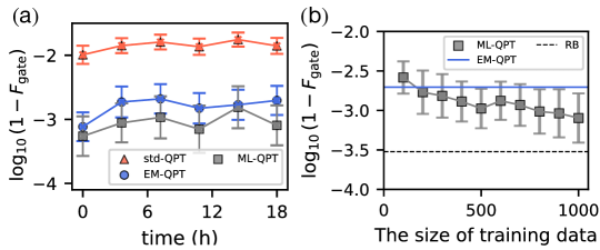
Figure 11: Stability and convergence. (a) The QPT infidelity as a function of time (over 18 hours) across the three investigated methods. For ML-QPT, the digital twin is trained on a data set of $10^{3}$ error matrices. (b) The infidelity of ML-QPT as a function of the size of the training data, where the training data is randomly sampled from the full data set of $10^{3}$ error matrices. Each data point is averaged over the same measurement data set comprising $10^{2}$ X gates. For comparison, we include the average gate fidelity of EM-QPT (solid blue line) and the RB fidelity (dashed line). Error bars in (a) and (b) correspond to the standard deviation of the QPT process for $10^{2}$ experimentally implemented X gates.

In this section, we analyze the stability of the trained model. A digital twin was first trained using a data set of $10^{3}$ samples. We then performed QPT six times over 18 hours, with each experiment comprising $10^{2}$ X-gate measurements and corresponding identity-gate measurements. In Fig. 11(a), we compare the performance of the three different methods over time. The results demonstrate that ML-QPT exhibits stability comparable to EM-QPT while achieving even higher accuracy.

Figure 11(b) examines the training data requirements. Non-repeating subsets of $10^{2}$ to $10^{3}$ points were randomly sampled from the full data set ($N=10^{3}$) to train the digital twin. Each model was evaluated on the same $10^{2}$ X gates via EM-QPT, with fidelities averaged over $10^{2}$ digital twin simulations of error matrices. The infidelity converges to $\sim 10^{-3}$ when the training set exceeds $5\times 10^{2}$ samples (error bars: standard deviation across $10^{2}$ X-gate measurements).