Interplay of localization and topology
in disordered dimerized array of Rydberg atoms

Abstract

Rydberg tweezer arrays provide a platform for realizing spin-1/2 Hamiltonians with long-range tunnelings decaying according to power-law with the distance. We numerically investigate the effects of positional disorder and dimerization on the properties of excited states in such a one-dimensional system. Our model allows for the continuous tuning of dimerization patterns and disorder strength. We identify different distinct ergodicity-breaking regimes within the parameter space constrained by our geometry. Notably, one of these regimes exhibits a unique feature in which non-trivial symmetry-protected topological (SPT) properties of the ground state extend to a noticeable fraction of states across the entire spectrum. This interplay between localization and SPT makes the system particularly interesting, as localization should help with stabilization of topological excitations, while SPT states contribute to an additional delocalization. Other regions of parameters correspond to more standard nonergodic dynamics resembling many-body localization.

Introduction –

Generic quantum many-body systems are believed to follow Eigenstate Thermalization Hypothesis (ETH) [Deutsch91, Srednicki94, Srednicki99]. Recent intensive studies of nonintegrable systems revealed several ergodicity-breaking phenomena such as many-body localization (MBL)[Fleishman80, Gornyi05, Basko06, Alet18], many-body quantum scars [Bernien17, Turner18, Serbyn21, Moudgalya22rev] or Hilbert Space Fragmentation [Khemani20, Moudgalya22rev, Kohlert23]. All these systems have one thing in common: ETH violating localized eigenstates are shortly-correlated or, in other words, they are characterized by an area-law entanglement. It has been suggested [Huse13] that the quantum order of ground state, such as Spontaneous Symmetry Breaking (SSB), Topological Order or Symmetry Protected Topological (SPT) order can be promoted to excited spectrum in area-law entangled phase such as MBL. Shortly afterwards, few such systems were indeed found [Chandran14, Bahri15, Decker20, Parameswaran18, Laflorencie22, Vasseur16, Kuno19].

While most of the disordered systems studied considered a local on-site disorder [Nandkishore15, Alet18, Abanin19, Sierant25], recently a progress in understanding of the phenomenology of ergodicity breaking in bond-disordered spin chains has been reached [Aramthottil24]. It was shown that the behavior of systems such as, e.g., random-bond XXZ, is better described by the real space renormalization group for excited states (RSRG-X) [Pekker14], rather than LIOMs language. RSRG-X captures nontrivial entanglement entropy distributions and sub-Poissonian mean gap ratio observed in such random bond models [Aramthottil24] for which the existence of LIOMs is ruled out. Motivated by that work, we explore here the possibilities of realization of SPT excited states in such LIOM-free models (see, however [Vasseur16, Kuno19]).

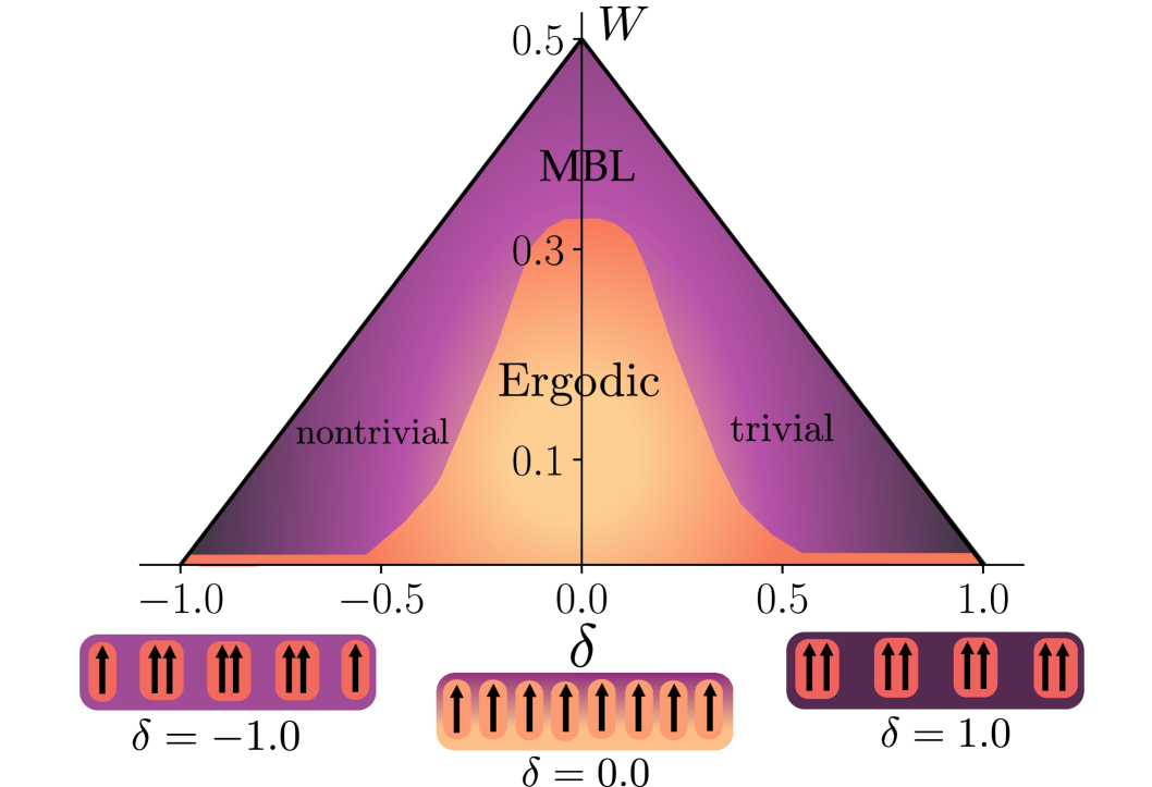
Figure 1: The qualitative phase diagram for the model in $\delta,W$ space where $\delta$ is the dimerization parameter in the model defined by (1) and (2) and $W$ is the positional disorder strength.

We investigate here a one-dimensional spin-1/2 lattice model inspired by experiments with arrays of Rydberg atoms kept in tweezers [Browaeys20], where, e.g., the first realization of a many-body SPT phase of interacting bosons in an artificial system was recently reported [Leseleuc2019]. We concentrate on the dipolar XY model as realized due to a direct dipole-dipole interactions between Rydberg states of different parity [Browaeys20, Chen23] and we consider a one-dimensional chain. Using a Rydberg tweezer platform one may realize different dimerization patterns combined with positional disorder, enabling access to different SPT phases and ergodic/ergodicity-breaking regimes.

Model –

Our model is defined by the Hamiltonian

$$H=J\sum_{i>j}\frac{1}{r_{ij}^{3}}\left(s_{i}^{x}s_{j}^{x}+s_{i}^{y}s_{j}^{y}\right),$$ (1)

where $J=1$ sets the energy unit (we use later a notation $J_{ij}\equiv J/r^{3}_{ij}$) and $s_{i}^{k}$, $k=x,y,z$ are spin-1/2 operators. Spins are placed at positions $r_{i}$ with $r_{ij}\equiv\left|r_{i}-r_{j}\right|$. We assume open boundary conditions (OBC).

Hamiltonian (1) obeys $U(1)$ symmetry, which corresponds physically to the conservation of a total magnetization along the $z$ direction. The second symmetry, crucial for the protection of SPT order, is represented by an antiunitary $S=\prod_{i}s_{i}^{x}\circ K$, where $K$ is a complex conjugation. This makes the symmetry group of our system $U(1)\times\mathbb{Z}_{2}^{T}$. Note that the coupling between spins is long-range decaying as a power law. In effect, after the Jordan-Wigner transformation, the Hamiltonian contains interacting terms [Leseleuc2019], so it should be treated exclusively as bosonic 1D interacting SPT system [Chen11, Chen11_2].

We introduce the disorder into our model by randomizing positions of spins. With SSH [Su79] logic behind, we distribute the positions of spins as

$$r_{i}=\left(i+\frac{\delta(-1)^{i+1}-1}{2}\right)a+i\hskip 1.29167ptD_{rb}+W_{i},$$ (2)

where parameter $\delta\in\left[-1,1\right]$ quantifies the degree of dimerization. We have the chain with paired spins in the bulk and two almost decoupled spins at the edges for $\delta=-1$ and all spins paired for $\delta=1$ - see Fig. 1, the corresponding regions are loosely called nontrivial and trivial, respectively. Random $W_{i}$ values are drawn from the uniform distribution $W_{i}\in[-W,W]$ and $D_{rb}$ is the Rydberg blockade diameter. Therefore, $\tilde{a}=a+{D}_{rb}$ gives the average distance between two neighboring spins. From now on, we fix $a=1$ and ${D}_{rb}=0.2$.

Assuming the straight line chain geometry we obtain the constraint on $W$ and $\delta$:

$$W\hskip 1.29167pt<\hskip 1.29167pta\cdot\min\left(\frac{1-\delta}{2},\frac{\delta+1}{2}\right),$$ (3)

leading, for fixed $a$ and $D_{rb}$, to a triangular parameter space – compare Fig. 1.

Localization properties

First, we benchmark the localization crossover depending on the disorder strength $W$ for a uniform pattern of spins ($\delta=0$). We work in the zero magnetization and even parity sector across the paper. To this end we use standard tools, finding the mean gap ratio and the mean half-chain entanglement entropy (EE) of eigenstates. The gap ratio is defined as $r_{k}=\frac{\min\{\delta_{k},\delta_{k+1}\}}{\max\{\delta_{k},\delta_{k+1}\}}$ (where $\delta_{k}=E_{k+1}-E_{k}$ is the difference between two consecutive eigenvalues of (1) and the average is taken over $1000$ eigenvalues in the middle of the spectrum and between $100$ for $L=20$ and $5000$ for $L=12$ different disorder realizations). The half chain EE is defined as $S_{ent}(L/2)=-\mathrm{Tr}(\rho\log_{2}(\rho))$ (where $\rho$ - density matrix obtained by tracing out the eigenstate over half of the chain). The results are plotted in panels (a) and (b) in Fig. 2. To diagonalize the Hamiltonian we employ exact diagonalization for $L\leq 16$ and POLFED [Sierant20polfed] for larger system sizes. One observes that both the mean EE and the mean gap ratio curves for different system sizes cross around $W\approx 0.33$, indicating a crossover from delocalized to localized character. A careful observer will notice significant size effects. Only for $L\geq 14$ for small disorder values, the expected ergodic dynamics with mean gap ratio corresponding to the gaussian orthogonal ensemble (GOE) are reached. On the localized side, even for the largest disorder, the Poissonian value 0.389 for $\langle r_{k}\rangle$ is not reached, staying above 0.4.

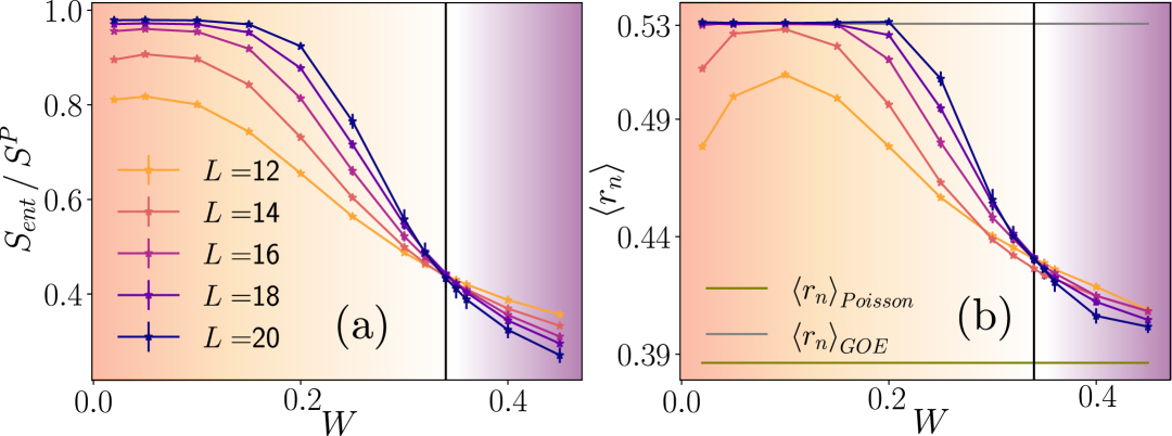
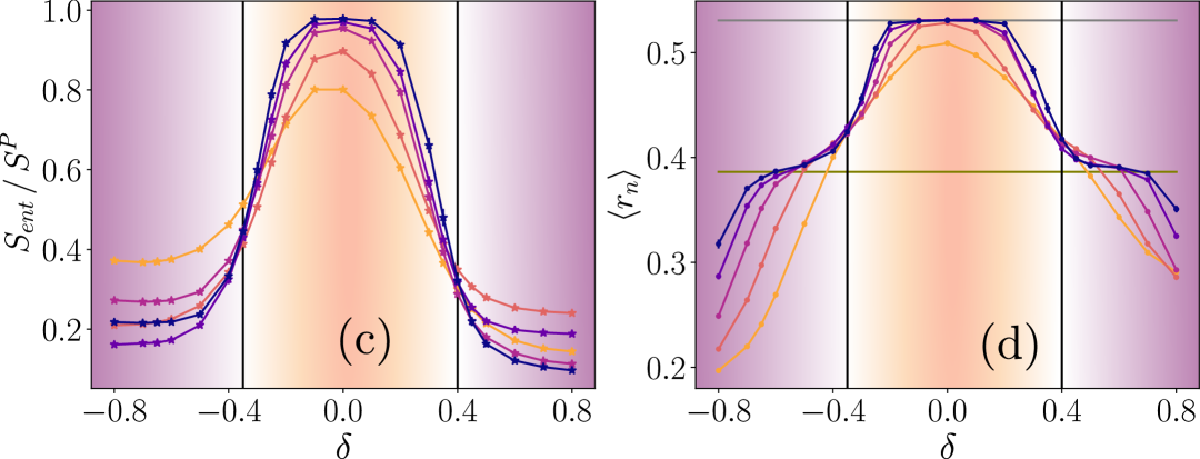
Figure 2: Half-chain Entanglement entropy $S_{ent}$ and the mean gap ratio $\braket{r_{n}}$ as a function of the disorder strength $W$ for fixed $\delta=0$ (a-b) and as a function of dimerization $\delta$ for fixed $W=0.1$ (c-d).

Next, we fix disorder strength $W=0.1$, corresponding to a delocalized regime for uniformly spaced spins, and vary the dimerization parameter $\delta$ - c.f. Fig.2(c-d). Three distinct phases may be observed. For small $\delta$, the system is delocalized with the mean gap ratio and the mean EE reaching values corresponding to GOE for systems of sufficient size. The mean EE and the mean gap ratio reveal two crossovers for $\delta$ sufficiently different from $0$ occurring for small disorder $W$ values. It should be noticed, that curves in Fig.2(c) in localized regimes have an unusual system size ordering due to the fact that we cut the system on strong/weak bonds depending on $L$ for EE calculations. In case of $W=0.1$ the crossings occur at $\delta\approx-0.35$ and $\delta\approx 0.4$. The resulting phases are localized as indicated by the mean gap ratio (sub-Poisonnian statistics was found also in [Decker20]) and sub-volume mean EE. Yet, they differ significantly for negative and positive dimerization, $\delta$. As discussed below, for $\delta<-0.35$ phase, a noticeable fraction of states across the entire excited spectrum shares symmetry-protected topological (SPT) properties of the ground state.

Real space renormalization group insight –

To gain insight into the form of eigenstates in nonergodic regimes, we use the real space renormalization group for excited states (RSRG-X) [Pekker14], an extension of the strong disorder renormalization group scheme [Dasgupta80, Fisher94] for excited states. This scheme works best for Hamiltonians constructed as the sum of operators that act on a few sites with a broad range of energy gaps [Protopopov20, Mohdeb22, Aramthottil24]. Our version is specifically adapted to a dimerized Hamiltonian; for a general scheme for long-range interacting systems, see [Zhao25].

Initially, the two-site operator with the largest coupling is identified in (1), as we have a dimerized form let us consider $i,j=i+1$ sites: $H_{ij}=\frac{J_{ij}}{2}(s_{i}^{+}s_{j}^{-}+s_{i}^{-}s_{j}^{+})$. In the resulting dim=4 subspace, the diagonalization gives eigenstates $\ket{\pm}_{ij}\equiv\frac{1}{\sqrt{2}}(\ket{\uparrow\downarrow}\pm\ket{\downarrow\uparrow})_{ij}$ and a degenerate subspace spanned by $\ket{Z_{+/-}}_{ij}\equiv\ket{\uparrow\uparrow}/\ket{\downarrow\downarrow}_{ij}$. In this new basis, one perturbatively modifies operators connected to sites $i,j$, of generic forms $H_{li},H_{lj},H_{ir},H_{jr}$. For $\ket{\pm}_{ij}$ states, the resulting operator takes the form $H_{lr}=\frac{[J_{li}(J_{jr}\pm J_{ir})+J_{lj}(J_{ir}\pm J_{jr})]}{2J_{ij}}(s_{l}^{+}s_{r}^{-}+s_{l}^{-}s_{r}^{+})$. The $l,r$ sites are again chosen by the strength of the coupling between them. In the degenerate subspace we have an additional possible choice of the basis that affects the functional form of $H_{lr}$. For example, the $\ket{Z_{\pm}}_{ij}$ leads to $H_{lr}=-\frac{[J_{li}J_{jr}+J_{lj}J_{ir}]}{2J_{ij}}(s_{l}^{+}s_{r}^{-}+s_{l}^{-}s_{r}^{+})\pm 2[\frac{J_{li}J_{lj}}{J_{ij}}s_{z}^{l}+\frac{J_{ir}J_{jr}}{J_{ij}}s_{z}^{r}]$ yielding chemical potential-like terms while $\frac{1}{\sqrt{2}}(\ket{Z_{+}}_{ij}\pm\ket{Z_{-}}_{ij})$ results in $H_{lr}=-\frac{[J_{li}J_{jr}+J_{lj}J_{ir}]}{2J_{ij}}(s_{l}^{+}s_{r}^{-}+s_{l}^{-}s_{r}^{+})\mp\frac{[J_{li}J_{ir}+J_{lj}J_{jr}]}{2J_{ij}}(s_{l}^{+}s_{r}^{+}+s_{l}^{-}s_{r}^{-})$ generating a pair-hopping term. The chemical potential term effectively creates domains of parallel spins, the pair-hopping term creates $Z-$exchanges: $\ket{Z_{\pm}}_{ij}\rightleftarrows\ket{Z_{\mp}}_{lr}$ that is chosen only if the energy gap associated with the exchange is greater than that of a domain with the least distance to the pair.

In this way four sites $l,i,j,r$ are replaced by two sites $l,r$ with effective operator $H_{lr}$ The procedure is called a decimation. Successive decimations involve more sites. Spanning all the chain and diagonalizing the last operator gives the estimation of eigenstates for a given path ${\cal P}$, defined by successive choice of basis states during decimations.

In the trivial regime, the bonds between sites $(2i-1,2i)$ will be the strong bonds leading to large energy gaps. Thus, the operators that are fixed in decimations will be on the sites occupied by these bonds. Depending on the path ${\cal P}$ chosen, either via cat states $\ket{\pm}$ or $Z$-subspace, this results in approximate eigenstates of the form $\ket{\Psi_{\mathrm{T}}}=\otimes_{\{j\}}\ket{\pm}_{2j-1,2j}\otimes_{\{i\}}(\cos(\varphi_{i})\ket{Z_{+}}_{2i-1,2i}+\sin(\varphi_{i})\ket{Z_{-}}_{2i-1,2i})$ where, $\{j\}$ are sites involving $\ket{\pm}$ and $\{i\}$ involving linear combinations (defined via $\varphi$) of $\ket{Z_{\pm}}$ states.

In contrast, in the non-trivial regime, the bonds between sites $(2i,2i+1)$ will be comparatively larger and produce the largest energy gaps. This leads to isolated spins at the boundaries that are connected to the rest by weak bonds only. Those will be coupled in the last decimation step. Once all relevant bonds in the bulk are fixed, the most relevant bonds associated with the edge sites will be the bond that directly connects them, of the energy scale $J\approx 1/(L\tilde{a})^{3}$, or the chemical potential bond from the nearby dimer, which will go as $J\approx[\delta a+\tilde{a}]^{3}/(m\tilde{a})^{6}$, where $m\tilde{a}$ is the distance to the nearby fixed $\ket{Z_{\pm}}$ domain. The cases of states where the direct connection dominates can have edge sites fixed as $\ket{\pm}_{1,L}$ or $\ket{Z_{\pm}}_{1,L}$. In the latter case, one can have exchanges with the bulk. We shall refer to both such types of states as $\ket{\Psi_{\mathrm{NT}}}$.

SPT properties –

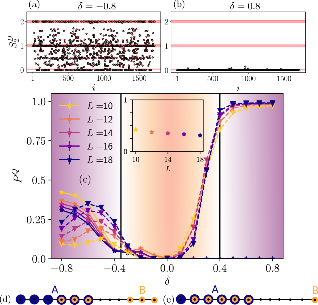
Figure 3: (a-b) The plots show $S^{D}_{2}$ for all states within the appropriate symmetry sector at $L=14$, for a single typical disorder realization for $W=0.1$ with $\delta=-0.8$ and $\delta=0.8$, respectively. (c) Fraction of states with $S^{D}_{2}=1,2$ is indicated by stars connected by solid line for different system sizes. Triangles connected by dashed lines represent the fraction of states with $S^{D}_{2}=0$. Data averaged over several disorder realizations for $W=0.1$. The inset shows the fraction of nontrivial states for $\delta=-0.8$. (d-e) Partitions used to define Disconnected entropy (4). Blue and orange circles denote sets $A$ and $B$, respectively.

Hamiltonian (1) is an extension of the bosonic version of the SSH model [Su79, Hasan10, Kane13, Shankar18, Batra20] by long-range hopping (that preserves the symmetries of the system). The ground states for negative/positive $\delta$, even in the presence of the positional disorder, are in nontrivial/trivial SPT phases (compare [suppl]). In the nontrivial phase ($\delta<0$), the ground state manifold is characterized by the presence of edge modes (with the corresponding 4-fold degeneracy in the open chain) and a long-range string order [Torre06, Berg08]. Additionally, these states can not be smoothly deformed into ground states coming from the trivial phase ($\delta>0$), without breaking the protecting symmetry or closing the gap.

The RSRG-X procedure, described above strongly suggests that our model in the ergodicity-breaking regimes hosts a significant fraction of short-correlated states of different topology across the whole excited spectrum.

Distinguishing between different SPT phases numerically is a challenging task [Pollmann12]. Recently, it was shown [Zeng16, Zengbook] that the long-range entanglement between edge states can identify nontrivial SPT order. That can be quantified by the so-called disconnected entropy [Zeng16, Fromholz20]:

$$S^{D}=S^{A}_{ent}+S^{B}_{ent}-S^{A\cup B}_{ent}-S^{A\cap B}_{ent},$$ (4)

where $S_{ent}^{C}$ is a bipartite entanglement entropy for partition $C$.

Typically, the construction of subsystems is done by a division of the chain into 4 parts, [Zeng16, Zengbook, Fromholz20, Micallo20] or more formally one can define $A=\left\{1,...L/2\right\}$ and $B=\left\{\lceil L/4\rceil+1,...L/2,\lfloor 3L/4\rfloor+1,...L\right\}$ – c.f. Fig.3(d) – where floor $\lfloor x\rfloor=\mathrm{max}\{z\in\mathbb{Z}|z\leq x\}$ and ceiling $\lceil x\rceil=\mathrm{min}\{z\in\mathbb{Z}|z\geq x\}$ are introduced to deal with system sizes which are not devisable by 4. For the reasons, which will be apparent below, we propose another way to divide our chain: $A=\left\{1,...L/2\right\}$, $B=\left\{2,...L/2,L\right\}$ as shown in Fig.3(e). Let us denote disconnected entropies corresponding to these conventions as $S^{D}_{1}$ for the original one and $S^{D}_{2}$ for our definition.

Consider first the sufficiently negative $\delta$. We expect to have $\ket{\Psi_{\mathrm{NT}}}$ eigenstates across the spectrum. Firstly if we fix $\ket{\phi}_{1,L}=\ket{\pm}$, these states will have the same construction as the nontrivial groundstate, and more complicated structures will be coming from bulk exchanges, which are analogous to triplon excitations studied in [Chandran14]. Such states will have $S^{D}_{1}=S^{D}_{2}=2$ indicating maximal correlations between edge sites. They can be interpreted as topologically nontrivial. The next significant family for the same parameters consists of the states$\ket{\Psi_{\mathrm{NT}}}$ with $\ket{\phi}_{1,L}=\ket{Z_{\pm}}$, which can be interpreted as a domain-wall in the bulk of the nontrivial SSH chain [Kane13]. These states have a quantized value of $S^{D}_{2}=1$, meaning that edge spins are coherently correlated, but entanglement is not maximal. For the original definition of $S^{D}_{1}$ it is more ambiguous, because we are looking at correlations between multiple sites close to the edges. If domain wall is formed in these areas, $S^{D}_{1}$ will give $2$, hence it is not distinguishing between these states and states from the first family.

Therefore, nontrivial short-entangled states (in the thermodynamic limit) are characterized by nonzero quantized values of the disconnected entropy, $S^{D}_{2}$. The numerical results for $S^{D}_{2}$ are shown in Fig. 3(a,c) (results for $S^{D}_{1}$ are shown in [suppl]). We plot the fraction of states with quantized, integer values of disconnected entropy

$$P^{Q}(S^{D}=k)=\left<{N_{k}}/{N}\right>,$$ (5)

where $N_{k}$ is the number of the states with $S^{D}\in[k-\epsilon,k+\epsilon]$, $k=0,1,2$, $N$ - the dimension of the corresponding symmetry block and averaging $\left<\cdot\right>$ is taken over disorder realizations. We set $\epsilon=0.05$ in all of our calculations. One may observe the presence of a significant number of states with $S^{D}_{2}=0$, suggesting that not all "product states" in this configuration of spins will develop coherent correlations between edges. In particular, states with non-integer values of $S^{D}$ have a more complicated entanglement structure, and, typically, larger entanglement entropy. On the other hand, a significant fraction of states has non-zero, quantized $S^{D}_{2}$ indicating their topological character. Importantly this fraction very slowly decays with the system size $L$ as shown in the inset of Fig. 3(c) suggesting that it may also exist in the thermodynamic limit. To estimate this fraction full spectra of (1) were needed, so $50$ disorder realizations were used for $L=18$. For a further, more detailed analysis of size effects see [suppl].

For sufficiently positive $\delta$ we expect formation of states $\ket{\Psi_{\mathrm{T}}}$. Again, deviations from the simple dimer product state structure are captured by more and more complicated exchanges of frozen spins on our dimers. $S^{D}_{2}$ will give $0$ for this type of states, because arrangement of coherent entanglement between first and last spins is impossible within this configuration. Strikingly, this picture is different for $S^{D}_{1}$. Frozen spin exchanges can happen at the ends of our chain and this will lead to $S^{D}_{1}=2$. Similar states with $S^{D}_{1}=1$ also may occur. For that reason, we defined $S^{D}_{2}$ as a more informative disconnected entropy measure.

Let us just mention that in the ergodic regime ($\delta$ around $0$) we expect to have arbitrary (unquantized) values of the disconnected entropy, because eigenstates across the spectrum are volume-law entangled.

Time dynamics

The RG picture is nicely confirmed by the time dynamics. Consider the time evolution of an initial state with alternate dimerizations of $\ket{\pm}$ states in the bulk, and frozen opposite spins at the edge sites: $\ket{\Psi}\equiv\ket{\uparrow}_{1}\ket{+}_{2,3}\ket{-}_{4,5}\cdots\ket{\downarrow}_{L}$. We take care that the state falls into the middle of the spectrum. In the strong disorder limit, this state can be seen as a linear combination of two approximate eigenstates suggested by RSRG-X: $\ket{\Psi}\equiv\frac{1}{\sqrt{2}}(\ket{\Psi_{1}}+\ket{\Psi_{2}})$, of the form $\ket{\Psi}_{1/2}\equiv\ket{\pm}_{1,L}\ket{+}_{2,3}\ket{-}_{4,5}\cdots\ket{-}_{L-2,L-1}$, with respective energy $E_{1}$ and $E_{2}$. As time evolves, the site-resolved magnetization at the edges, ${s}_{1}^{z},{s}_{L}^{z}$ indeed reveal oscillations with a period $T=\frac{2\pi}{E_{1}-E_{2}}$ as shown in Fig. 4(a) for a single disorder realization. Figure 4(b) confirms that the disorder-averaged period of oscillations scales as a third power of the system size as expected from the tunneling part of the Hamiltonian (1). Another example of time dynamics supporting the RSRG-X construction is shown in [suppl].

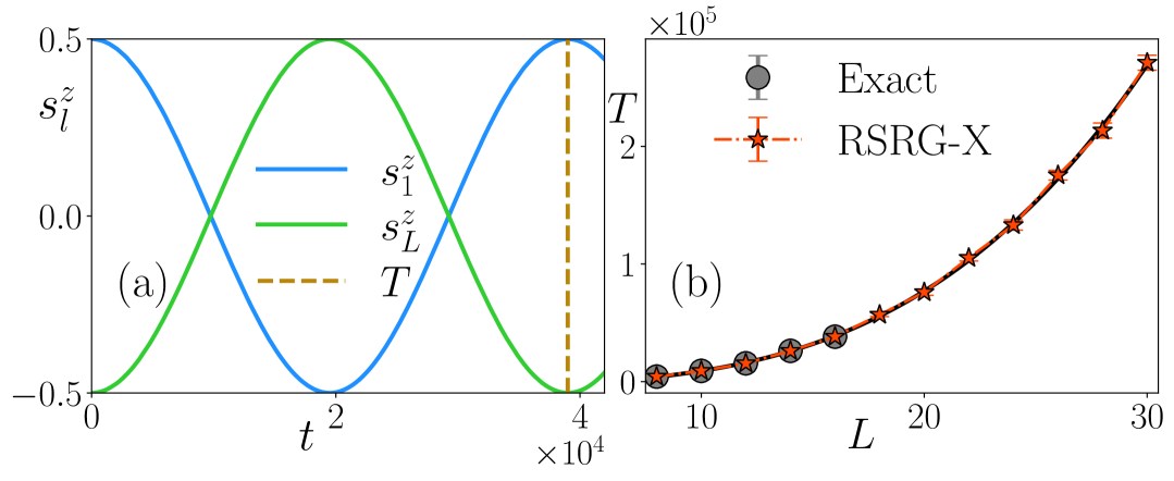
Figure 4: (a) Represents oscillations observed in site-resolved magnetization, $s_{l}^{z}$, of the first and last sites for a single disorder realization for the quench state, $\ket{\Psi}$, in the nontrivial regime ($L=16$). The dashed line indicates the time period, $T$, predicted by RSRG-X. (b) Disorder-averaged values, with a minimum of 200 realizations, for such $T$s obtained from both exact and RSRG-X for various system sizes are plotted. The black curve represents a third-order polynomial fit. The system parameters for both plots are $\delta=-0.8$ and $W=0.1$.

Conclusions –

We have presented a spin model of a long-range power-law interacting system that reveals nontrivial topological excited states due to disorder in spin positions. Depending on the degree of dimerization as well as the magnitude of the positional disorder, the model reveals either a typical MBL (spin-glass) phase for strong disorder and weak dimerization or two localized phases for strong dimerization with globally different properties. One of them, in which the edge sites are strongly coupled to the bulk, is dominated by topologically trivial states. On the other hand, if the edge spins are weakly coupled to the bulk (as in the interaction-free SSH model), a different phase dominated by non-trivial topological states is obtained. The structure of states and their time dynamics may be easily understood by the RSRG-X technique. The advantage of the model studied is that it may be directly realized experimentally for Rydberg atoms kept in optical tweezers, systems recently studied very efficiently. Let us mention that adding additional $z-z$ interactions to the model, such as that resulting from van der Walls interactions [Homeier2025, Zeybek23] significantly changes its properties, making non-trivial states less abundant [suppl].

Supplemental Material: Interplay of localization and topology in disordered dimerized array of Rydberg atoms

S-I Properties of the model

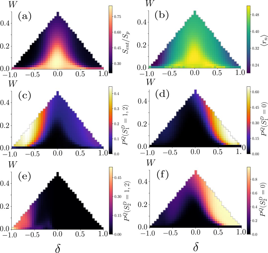
Figure S1: Scans of the $(\delta,W)$ plane for $L=14$, $a=1$, $D_{rb}=0.2$. Top row: (a) mean gap ratio and (b) the rescaled entanglement entropy. Middle row: (c) fraction of states with disconnected entanglement entropy $S^{D}_{1}=1,2$, (d) fraction of states with $S^{D}_{1}=0$. Bottom row (e-f) 0 same as the middle row but for other definition of disconnected entropy $S^{D}_{2}$.

As discussed in the main text, for fixed spacing $a=1$ and Rydberg blockade diameter $D_{rb}=0.2$, the model is effectively characterized by two parameters - the strength of the disorder $W$, the dimerization parameter $\delta$. $\delta$ determines the mean spacing between odd-even and even-odd sites, $\delta=0$ corresponds to no dimerization. Due to (3) the space of parameters takes a triangular shape as shown in Fig. S1. We present here the data for $L=14$ averaged over $1000$ disorder realizations for the whole parameter space. The top row (a-b) of Fig. S1 shows “standard” measures used to describe properties of the system - the half-chain entanglement entropy (scaled by the Page value) and the mean gap ratio. Both quantities reveal transitions from small dimerization (i.e. $\delta$ close to 0) and disorder corresponding to delocalized behavior to a localized phase for sufficient dimerization or for large disorder.

Figure S1(c-f) presents data for the disconnected entropy (4) for two different ways of partitioning our system: $S^{D}_{1}$ and $S^{D}_{2}$. The fraction of states with quantized, integer values of disconnected entropies $P^{Q}$ is shown there. Note that integer values appear because we define the entropy with base-2 logarithm. We plot

$$P^{Q}(S^{D}=k)=\left<{N_{k}}/{N}\right>,$$ (S1)

where $N_{k}$ is the number of the states with $S^{D}\in[k-\epsilon,k+\epsilon]$, $k=0,1,2$, $N$ - the dimension of the corresponding symmetry sector and averaging $\left<\cdot\right>$ is taken over disorder realizations. We set $\epsilon=0.05$ in all of our calculations.

Regions of nonzero $P^{Q}$ are vastly different for $S^{D}_{1}$ and $S^{D}_{2}$. $S^{D}_{1}$ states with $k=1,2$ populate almost whole parameter space (except the ergodic region), since $S^{D}_{1}$ captures correlations between bigger partitions around the edges (recall its definition in the main text). Not all of these long-range correlations have a topological nature, because they do not necessarily involve decoupled edge spins. Nevertheless, $S^{D}_{1}$ reveals the long-range entanglement structure of the excited eigenstates in our model. We further plot $P^{Q}(S^{D}_{1})$ for different system sizes for horizontal cut $W=0.1$ in Fig.S2 (in the similar fashion to the Fig.3(c) in the main text).

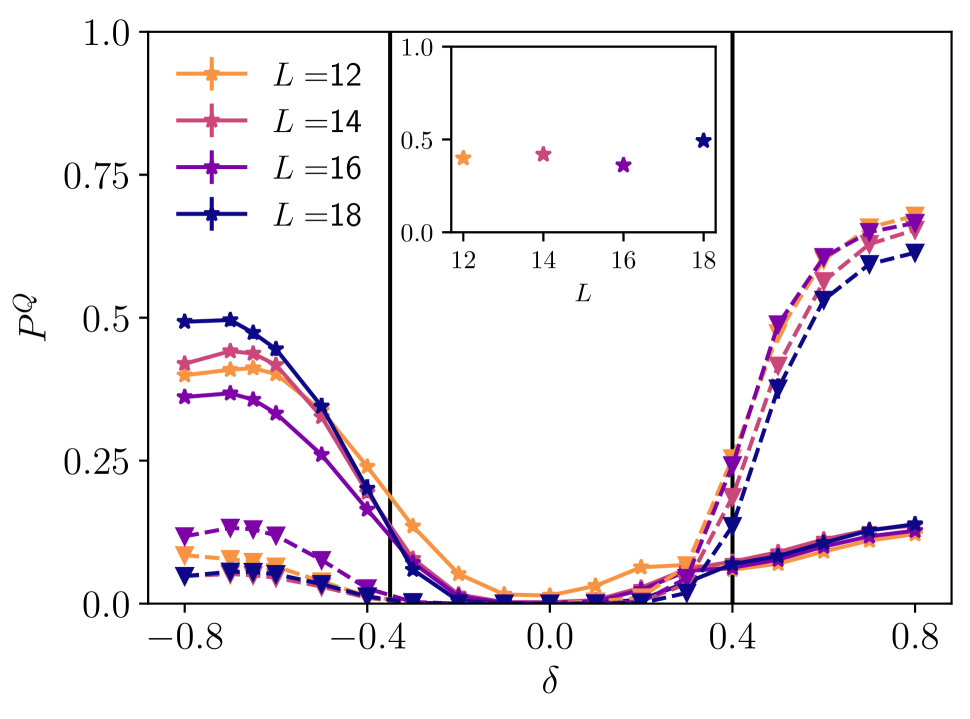
Figure S2: Fraction of states with $S^{D}_{1}=1,2$ is indicated by stars for different system sizes. Triangles connected by dashed lines represent a fraction of states with $S^{D}_{1}=0$. Data averaged over several disorder realizations for $W=0.1$. The inset shows the fraction of states with $S^{D}_{1}=1,2$ for $\delta=-0.8$, showing weak system size dependence.

For $S^{D}_{2}$, the corresponding region with a significant fraction of states with $k=1,2$ is smaller, such states mainly concentrate in the left bottom corner of the parameter space. It is worth noting, that $S^{D}_{2}$ also shows quantized behavior for the nondisordered case $W=0.0$ due to the restoration of the reflection (around the middle of the chain) symmetry, which creates long-range entanglement picked up by $S^{D}_{2}$. The corresponding eigenstates do not have the same properties and simple structure as previously discussed ones coming from disordered (1), so this false signature can be regarded as a drawback of $S^{D}_{2}$.

For completeness, the behavior of the average $S^{D}_{2}$ in the ground state is plotted in Fig. S3. One can see that, away from $\delta=0$, it quickly saturates to zero for positive $\delta$, while the “pure” value of $2$ for negative $\delta$ is obtained for sufficiently small $\delta$.

Figure S3: Average disconnected entropy $S^{D}_{2}$ as function of $\delta$ for different system sizes.

Once again, we emphasize that only $S^{D}_{2}$ distinguishes between topologically trivial and nontrivial states beyond ground state manifold, because it captures the entanglement of the edge spins. Shortly-correlated states that have (for finite system sizes) some long-range entanglement that do not involve decoupled edge states, are smoothly connected to trivial product states.

S-II System size scalings

The significance of our finite-size simulations can be seen in the extrapolation of the probed system sizes to infinity. The dependence of $P^{Q}(S^{D}_{1,2})$ on the inverse of the system size $L$ is shown in Fig. S4. Each row compares the fraction of states, $P^{Q}(k)$, for $S^{D}_{1}$ and $S^{D}_{2}$ for $W=0.1$ and $\delta=-0.8$. In all cases shown numerical data are plotted using box representation, where orange line is a median of the samples, boxes correspond to ranges between first quartile ($Q_{1}$) and third ($Q_{3}$) and whiskers extend from $Q_{1}-\frac{3}{2}|Q_{1}-Q_{3}|$ to $Q_{3}+\frac{3}{2}|Q_{1}-Q_{3}|$. All linear fits are accompanied with shaded regions that show propagation of error away from data points.

Panels (a-b) focus on integer value $k=2$ for $S^{D}_{1,2}$. For $S_{2}^{D}$ (left panel) we also present the predictions of RSRG-X calculations that show quite accurate agreement with numerics coming from exact diagonalization. The numerical values are given in Table 1. Linear fits (with a shaded area indicating uncertainty limits) to the numerical data for $S^{D}_{2}$ (a) and $S^{D}_{1}$ (b) reveal a significant fraction of states with $k=2$ in infinite system size extrapolation limit.

Similar data, but for the case of $S^{D}_{1,2}=1$ are shown in the middle row of Fig. S4. As in a former case, one observes strong signatures of a significant fraction of nontrivial states for both disconnected entropies. Finally, the fraction of states with quantized to zero values of $S^{D}_{1,2}$ is presented in the bottom row - panels (e-f), together with the corresponding linear regression lines.

Let us stress again that the analysis presented in Fig. S4 reveals that a significant fraction of states with all three possible quantized values of disconnected entropy persists in the large $L$ limit for both definitions of $S^{D}$.

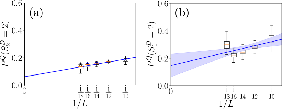
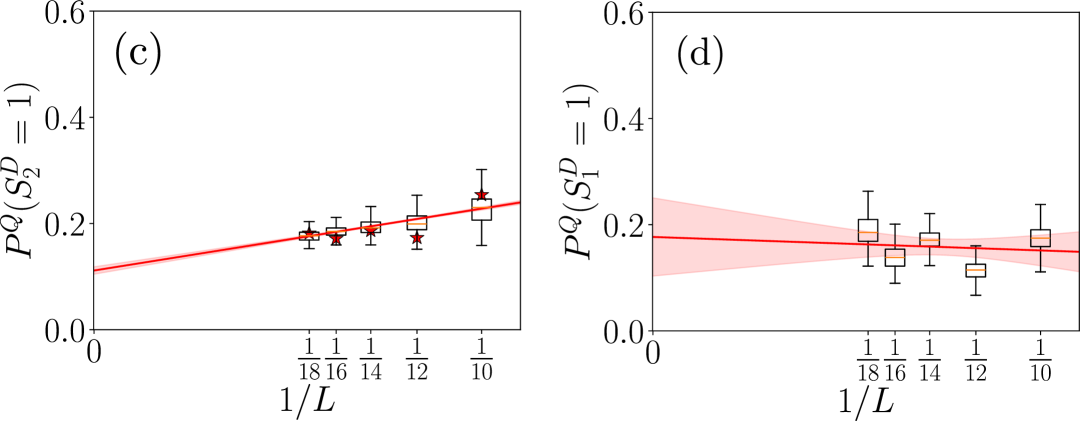
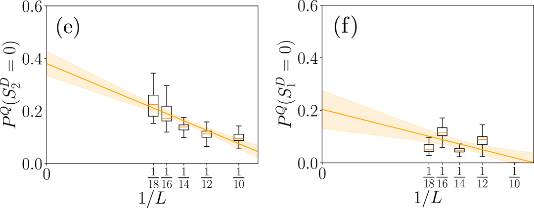
Figure S4: Scaling of the fraction of states with quantized values of $S^{D}_{1}$ and $S^{D}_{2}$ in the spectrum as a function of the inverse of the system size for $\delta=-0.8$ and $W=0.1$. Additionally, stars illustrate RSRG-X predictions for $P^{Q}(S^{D}_{2}=2)$ and $P^{Q}(S^{D}_{2}=1)$ in (a) and (c) respectively.

Table 1: Comparison of numerical results and RSRG-X predictions for $P^{Q}(S^{D}_{2})$ at $\delta=-0.8$ and $W=0.1$ point in the parameter space. Errors $\sigma$ are calculated using (S2).

$L$	$\braket{P^{Q}(S^{D}_{2}=2)}$	$\sigma(P^{Q})$	$P^{Q}_{RSRG-X}$
10	0.19108	0.00024	0.19048
12	0.16770	0.00016	0.17316
14	0.15420	0.00039	0.16317
16	0.14375	0.0010	0.15664
18	0.13198	0.0028	0.15204
$L$	$\braket{P^{Q}(S^{D}_{2}=1)}$	$\sigma(P^{Q})$	$P^{Q}_{RSRG-X}$
10	0.23062	0.00027	0.25396
12	0.20396	0.00030	0.17316
14	0.19455	0.00052	0.18648
16	0.18598	0.00086	0.17156
18	0.17649	0.0017	0.18165

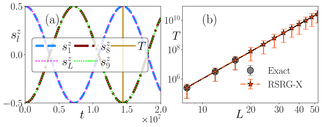
Figure S5: (a) Oscillations observed in site-resolved magnetizations, $s_{l}^{z}$, of the first and last sites for a single disorder realization for the quench state, $\ket{\Psi}$, in the nontrivial regime ($L=16$). Similar oscillations appear for spins located in the middle of the chain. The bold line indicates the period, $T$, predicted by RSRG-X. (b) Disorder-averaged values, with a minimum of 100 realizations, for the oscillation period obtained from both exact evolution and RSRG-X for various system sizes are plotted in a log-log scale. The straight line fit yields $\ln(T)=6.17\ln(L)-0.35$. The system parameters for both plots are $\delta=-0.8$ and $W=0.1$.

S-III Averaging and uncertainty calculations

To perform disorder averaging we use $5000,1000,300,400,100$ realizations for the respective system sizes $12,...,20$ in case of the vertical cut in the parameter space in the main text (Fig2(a-b)). Since horizontal cut is better converging Fig2(c-d) we used a bit smaller corresponding realization numbers $5000,1000,300,160,100$. In case of the Fig. 3 for $L=18$, only $50$ realizations are used from the full ED.

The error bars on all plots (except Fig. S4) are calculated using the formula for the standard error of the mean over disorder realizations.

$$\sigma(x)=\sqrt{\frac{\left<(x-\bar{x})^{2}\right>}{N_{d}}},$$ (S2)

where $N_{d}$ is number of disorder realizations and $\bar{x}$ denote disorder average.

S-IV Time dynamics with edge bulk exchanges

Apart from the example given in the main text, we show here another manifestation of the accuracy of the physical picture obtained using the RSRG-X scheme by considering time dynamics of an initial state of the form $\Psi\equiv\ket{\uparrow}_{1}\otimes\ket{-}_{2,3}\otimes\cdots\otimes\ket{Z_{-}}_{\frac{L}{2},\frac{L}{2}+1}\otimes\ket{+}_{\frac{L}{2}+2,\frac{L}{2}+3}\cdots\otimes\ket{\uparrow}_{L}$. This state, with energy lying in the middle of the spectrum, may be considered as a superposition of two $\ket{Z}$ edge-bulk exchange states. Looking at the time-evolution of this state one finds the oscillations between the edge $\ket{Z_{+}}_{1,L}$ and the $\ket{Z_{-}}_{\frac{L}{2},\frac{L}{2}+1}$ as shown for a particular disorder realization in Fig. S5(a). Figure S5(b) presents the average period, $T$, found after disorder averaging. As the leading energy scale difference between the eigenstates that form such a state is just $\frac{J_{1\frac{L}{2}+1}J_{\frac{L}{2}+1L}}{J_{\frac{L}{2}\frac{L}{2}+1}}$, the associated period, $T$, is expected to grow as $\propto L^{6}$ as verified by the fit obtained in Fig. S5 (b).

S-V Possible extensions

As mention in the main text a typical examples of Rydberg atom tweezer arrays without disorder are often well approximated by the pure XY model [Browaeys20, Chen23]. Arranging for the positional disorder is then easy by rearrangement of tweezers. It is interesting, however, to consider an enlarged family of models turning on $z-z$ coupling. Already in [Vasseur16] on the basis of RG considerations and numerical results it was shown that inclusion of $z-z$ couplings that decay in the same fashion as tunnelings (in our case $\propto\frac{1}{r^{3}}$) will destroy all of interesting features at the finite energy density. Following the recent approaches of [Homeier25] and [Zeybek23], we also check whether the same holds for models that combine tunnelings that scale as $\propto 1/r_{ij}^{3}$ arising from direct dipole-dipole interactions between Rydberg states of different parity and van-der-Waals interaction terms scaling as $\propto 1/r_{ij}^{6}$. This behavior is described by the Hamiltonian:

$$H=J\sum_{i>j}\frac{1}{r_{ij}^{3}}\left(s_{i}^{x}s_{j}^{x}+s_{i}^{y}s_{j}^{y}\right)+\Delta\sum_{i>j}\frac{1}{r_{ij}^{6}}s_{i}^{z}s_{j}^{z},$$ (S3)

We set $\Delta=1.0$ and calculate $P^{Q}(S^{D}_{2})$ for the horizontal cut in the parameter space $W=0.1$ - Fig. S6(a). We can see that region with positive dimerization parameter $\delta$ behaves very similarly to $\Delta=0$ case, but the behavior for the negative $\delta$ is now different. Firstly, the fraction of states with $S^{D}_{2}=0$ is now more prominent (in the large $L$ limit it goes to $85\%$). Secondly, the fraction of states with $S^{D}_{2}=1,2$ is now more modest. Moreover, the data for $\delta=-0.8$ plotted in Fig. S6(b) indicates that this fraction vanishes with $L$ very quickly. For comparison, we plot a fraction of states that have $S^{D}_{2}=2$ and do not involve any bulk exchanges (having only $\ket{\pm}$ terms in the bulk) as a purple curve. It behaves very similarly to $P^{Q}(S^{D}_{2}=2)$ indicating a finite size effect, not extensive with the system size.

The dependence of $P^{Q}$ on $\Delta\in[0,1]$ may also be analyzed - compare Fig. S6(c). It is apparent that a qualitative change occurs around $\Delta=0.1$. For larger $\Delta$ similar behaviour as for $\Delta=1$ is observed - with increasing system size the fraction of states with $S^{D}_{2}=0$ increases while those with long-range entanglement and $S^{D}_{2}=2$ goes down. For small $\Delta$ the trend for states with $S^{D}_{2}=0$ is reversed and the fraction of “interesting” states decays much slower.

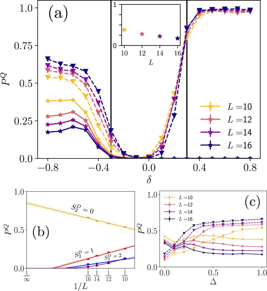
Figure S6: (a) Assuming $\Delta=1.0$ in (S3) fraction of states with $S^{D}_{2}=1,2$ is indicated by stars for different system sizes. Triangles connected by dashed lines represent a fraction of states with $S^{D}_{1}=0$. Data averaged over several disorder realizations for $W=0.1$. The inset shows the fraction of states with $S^{D}_{2}=1,2$ for $\delta=-0.8$. (b) Scaling of $P^{Q}(S^{D}_{2})$ with $\frac{1}{L}$ for $\delta=-0.8$. Purple points show fraction of states without bulk exchanges. (c) Dependence of $P^{Q}$ on $\Delta$ for $W=0.1$ and $\delta=-0.8$.