SmartUT: Receive Beamforming for Spectral Coexistence of NGSO Satellite Systems

Abstract

In this paper, we investigate downlink co-frequency interference (CFI) mitigation in non-geostationary satellites orbits (NGSOs) co-existing systems. Traditional mitigation techniques, such as Zero-forcing (ZF), produce a null towards the direction of arrivals (DOAs) of the interfering signals, but they suffer from high computational complexity due to matrix inversions and required knowledge of the channel state information (CSI). Furthermore, adaptive beamformers, such as sample matrix inversion (SMI)-based minimum variance, provide poor performance when the available snapshots are limited. We propose a Mamba-based beamformer (MambaBF) that leverages an unsupervised deep learning (DL) approach and can be deployed on the user terminal (UT) antenna array, for assisting downlink beamforming and CFI mitigation using only a limited number of available array snapshots as input, and without CSI knowledge. Simulation results demonstrate that MambaBF consistently outperforms conventional beamforming techniques in mitigating interference and maximizing the signal-to-interference-plus-noise ratio (SINR), particularly under challenging conditions characterized by low SINR, limited snapshots, and imperfect CSI.

I INTRODUCTION

Satellite communications (SatCom) will play a vital role in next-generation wireless networks by providing service to vast areas that lack terrestrial network coverage, especially with the rapidly growing Low-Earth orbit (LEO) mega-constellations [1]. These constellations are distributed in the Non-Geostationary Satellites orbits (NGSOs) and must manage co-existence strategies for sharing the limited spectrum [2]. Despite the proactive coordination efforts established by the International Telecommunication Union (ITU) among NGSO operators [3], there remains a risk of unintentional co-frequency interference (CFI), especially in the Ku/Ka bands where tens of thousands of NGSOs operate, potentially causing severe quality of service (QoS) degradation [4]. Thus, advanced interference avoidance and mitigation techniques that ensure both low complexity and efficient mitigation of unintentional interference in NGSO spectrum co-existence scenarios are needed.

User terminals (UTs) planar arrays are becoming popular because they can be used to steer the receiver electronically towards the moving satellite line-of-sight [5]. This work focuses on the adaptive beamforming (ABF) techniques on the UT side, where low complexity and fast adaptation are needed (due to the time-varying nature of the scenario). The goal is to generate antenna weights to accurately steer the main lobe towards the signal of interest (SOI) locations while minimizing the antenna gain towards interference locations.

Conventional correlation-based ABF methods, such as the Capon beamformer, also known as Minimum Variance Distortionless Response (MVDR) [6], rely on knowledge of the covariance (or correlation) matrix of the received signals. The covariance matrix is typically estimated using snapshots of the received signals, and accurate computation of the inverse covariance matrix is key to nulling interferers while preserving the SOI. Furthermore, this approach relies on channel state information (CSI) to constrain the beamformer towards the SOI direction. Moreover, traditional ABF’s main drawbacks are the high computational complexity involved in the weight calculation and the iterative nature of the algorithms, which makes the temporal response of the fast-moving satellites a critical concern.

Deep learning (DL)-based beamforming techniques have emerged as a potential solution to the traditional beamforming techniques’ drawbacks [7]. DL-based beamforming typically replaces or augments the classical weight calculation with a neural network that directly outputs beamforming weights. In this context, the authors in [8] compared the performance of an encoder-based beamformer, a convolutional neural network (CNN) and MVDR approaches in terms of signal-to-interference-plus-noise ratio (SINR) for LEO satellites communication systems; these approaches rely on supervised learning, which requires per definition input-output pairs. Obtaining such labeled data can be challenging due to the unpredictable environments of NGSOs, making the ground truth difficult to ascertain. In [9], the authors introduced an unsupervised deep neural network (DNN) beamforming (NNBF) model for the terrestrial uplink sum-rate maximization problem; the CSI was used as an input, but in the CFI case, only the desired CSI can be estimated. Furthermore, such a model might be sensitive to imperfect CSI scenarios.

Figure 1: Desired satellite downlink (green) with aggregated interference from a second independent NGSO constellation (red).

In this paper, we propose an unsupervised DL-based beamformer approach using Mamba state space models (SSMs) layers [10]. These layers effectively capture both spatial and temporal features from the input data that may be relevant to generating the correct beamforming weight vectors. Mamba-based beamformer (MambaBF) can be deployed on the UT side for more energy-efficient training and inference rather than on-board training [10615457], for assisting downlink CFI mitigation in NGSO communications. MambaBF is trained using the available received array snapshots as input to produce a beamforming weight vector that can maximize SINR by nulling interference directions.

II SYSTEM MODEL

We investigate CFI between two coexisting NGSO satellite constellations, as illustrated in Fig.1. In particular, we consider a desired satellite ($\mathrm{DS}$) serving a fixed UT, and some interfering satellites ($\mathrm{ISs}$) serving users in close vicinity of the UT location and therefore, pointing their signal power towards the nearby UT location. Our focus in this work is on the UT-side receive beamforming strategy, designed to avoid unintentional interference from other satellites.

II-A Channel and signal models

Consider the uniform planar array (UPA) at the UT lying in the $xy$-plane with $M_{x}\times M_{y}$ antenna elements on the $x$ and $y$ axes respectively, and the array size $M=M_{x}M_{y}$. Therefore, the UT array response vector can be written as [11],

$$\mathbf{v}(\phi,\theta) =\frac{1}{\sqrt{M}}\left[1,\cdots,e^{j\frac{2\pi}{\lambda}d(m_{x}\sin\phi\cos\theta+m_{y}\sin\theta)},\cdots,\right.$$ (1)

$$\left.e^{j\frac{2\pi}{\lambda}d((M_{x}-1)\sin\phi\cos\theta+(M_{y}-1)\sin\theta)}\right]^{T}\in\mathbb{C}^{M},$$

where $d$ is the inter-element spacing, $0\leq m_{x}<M_{x}$ and $0\leq m_{y}<M_{y}$ are the antenna indices in the $xy$-plane, $\phi$ and $\theta$ are the azimuth and the elevation angles respectively, representing the directions of arrival (DoAs). For notational brevity, we define a DoA as $\varphi\triangleq(\phi,\theta)$.

We are modelling a scenario where the $\mathrm{DS}$ transmits a signal ($s_{x}\in\mathbb{C}$) with $\mathbb{E}\{s_{x}s_{x}^{H}\}=1$ to its UT. Eventually, $K(K<M)$ interfering satellites ($\mathrm{IS}_{k},\quad k\in 1,\cdots,K$) are visible to the UT and unintentionally transmit an interference signal ($s_{i,k}\in\mathbb{C}$) towards it. When placing the UT in an obstacle-free elevated space as recommended by many operators (e.g., STARLINK [5]), the line-of-sight (LoS) component becomes dominant, thus the non-LoS (NLoS) propagation components can be ignored. Assuming $\mathrm{DS}$’s Doppler shift is compensated for at the UT, we define the statistical time-varying channel state information (sCSI) model between the $\mathrm{DS}$ satellite and the UT at time instant $t$ and frequency $f_{c,d}$ as follows[12],

$$\mathbf{h}_{d}=\chi_{d}\cdot\mathbf{v}_{d}(\varphi_{d})\in\mathbb{C}^{M},$$ (2)

where $\chi_{d}=\sqrt{P_{d}L_{d}G_{d}^{ut}(\varphi_{d})}$ is the channel gain, and $P_{d}$, $G_{d}^{ut}(\varphi_{d})$ are the $\mathrm{DS}$ Equivalent Isotropic Radiated Power (EIRP), and the maximum UT receive gain at $(\varphi_{d})$ direction. $L_{d}=(\frac{\lambda_{d}}{4\pi r_{d}})^{2}$ is the free space path loss inverse, $r_{d}$ is the slant range between UT and $\mathrm{DS}$, and $\lambda_{d}$ is the wavelength. Accordingly, the effective channel vector for the $k^{th}$ interfering satellite $\mathrm{IS}_{k}$ to UT receiver can be derived as,

$$\mathbf{h}_{i,k}=\chi_{k}\cdot\mathbf{v}_{k}(\varphi_{k}).$$ (3)

where $\chi_{k}=\sqrt{P_{k}L_{k}G_{k}^{ut}(\varphi_{k})}$. The UT array receiving gain $G^{ut}(\varphi)$ can be obtained as follows,

$$G^{ut}(\varphi)=\eta^{ut}D^{ut}(\varphi).$$ (4)

where $\eta^{ut}$, $D^{ut}$ are the UPA antenna efficiency and the directivity towards $\varphi$ direction. Note that the channel model adopted in (2) and (3) is applicable over a specific coherence time ”$t$” where the relative positions of the satellites and UT do not change significantly, and the physical channel parameters remain invariant. In this work, we simulate a constitutive sequence of coherence times for the sake of adaptability. Assuming that the UT array at the time instant $t$ can capture $L$ total snapshots, the $l^{th}$ snapshot vector can be expressed as,

$$\mathbf{y}[l]=\mathbf{h}_{d}s_{x}[l]+\mathbf{H}_{i}\mathbf{S}_{i}[l]+\mathbf{n}[l]\quad\in\mathbb{C}^{M},$$ (5)

where $\mathbf{H}_{i}\triangleq\left[h_{i,1};h_{i,2};\dots;h_{i,K}\right]\in\mathbb{C}^{M\times K}$, and $\mathbf{S}_{i}\triangleq\left[s_{i,1};s_{i,2};\dots;s_{i,K}\right]\in\mathbb{C}^{K}$, here $\mathbf{n}\in\mathbb{C}^{M}$ presents the additive white Gaussian noise (AWGN) at the UT receiver with i.i.d. $\mathcal{CN}(0,\sigma_{n}^{2}=\kappa T^{ut}BW_{d})$, where $\kappa$, $T^{ut}$, and $B_{d}$ are the Boltzmann constant, equivalent noise temperature of the UT, and $\mathrm{DS}$ signal bandwidth, respectively.

II-B Traditional beamforming techniques

For the UT to recover $\mathrm{DS}$ signals, we need to design a beamformer weight vector $\mathbf{w}\in\mathbb{C}^{M}$ with the objective of steering the UT main beam towards $\varphi_{0}$ direction and eliminating ”null” interference coming from $\varphi_{K}$ directions. The estimated signal after ($\hat{s}\in\mathbb{C}$) after applying $\mathbf{w}$ is,

$$\hat{s}[l]=\mathbf{w}^{H}\mathbf{y}[l]=\mathbf{w}^{H}\mathbf{h}_{d}s_{x}[l]+\mathbf{w}^{H}\mathbf{H}_{i}\mathbf{S}_{i}[l]+\mathbf{w}^{H}\mathbf{n}[l].$$ (6)

When we know the covariance matrix of a single snapshot $\mathbf{R}[l]\triangleq\mathbb{E}\{\mathbf{y}[l]\mathbf{y}^{H}[l]\}$, the beamformer $\mathbf{w}$ can be obtained by maximizing the output SINR [6],

$$\mathrm{SINR}_{\text{out}}[l]=\frac{\mathbf{w}^{H}\mathbf{R}_{d}[l]\mathbf{w}}{\mathbf{w}^{H}\mathbf{R}_{i+n}[l]\mathbf{w}},$$ (7)

where $\mathbf{R}_{d}=\mathbf{h}_{d}\mathbf{h}_{d}^{H}\in\mathbb{C}^{M\times M}$, $\mathbf{R}_{i+n}=\mathbf{H}_{i}\mathbf{H}_{i}^{H}+\sigma_{n}^{2}\mathbf{I}_{M}\in\mathbb{C}^{M\times M}$ are the desired covariance matrix and the interference-plus-noise covariance matrix, respectively.

The problem of maximizing (7) is mathematically equivalent to the MVDR beamforming problem [13]. In particular, the MVDR beamformer minimizes UT array input power while maintaining unity gain in $\mathrm{DS}$ direction,

$$\mathbf{w}_{\text{MVDR}}=\arg\min_{\mathbf{w}}\mathbf{w}^{H}\mathbf{R}\mathbf{w}\quad\text{subject to}\quad\mathbf{w}^{H}\mathbf{v}_{d}=1,$$ (8)

This optimization problem leads to the following weights for the beamformer $\mathbf{w}_{\text{MVDR}}=\frac{\mathbf{R}^{-1}\mathbf{v}_{d}}{\mathbf{v}_{d}^{H}\mathbf{R}^{-1}\mathbf{v}_{d}}$. In the finite sample case, $\mathbf{R}$ is unavailable; it is usually replaced by the sample covariance matrix $\hat{\mathbf{R}}$ for $L$ total snapshots, [14]

$$\hat{\mathbf{R}}=\mathbb{E}\{\mathbf{Y}\mathbf{Y}^{H}\}=\frac{1}{L}\sum_{l=1}^{L}\mathbf{y}[l]\mathbf{y}^{H}[l],$$ (9)

where $\mathbf{Y}=\left[\mathbf{y}[1],\mathbf{y}[2],\cdots\mathbf{y}[L]\right]\in\mathbb{C}^{M\times L}$. When $\hat{\mathbf{R}}$ is used to formulate (8), the solution is then called sample matrix inversion (SMI)-based minimum variance beamformer and is given by $\mathbf{w}_{\text{SMI}}=\frac{\hat{\mathbf{R}}^{-1}\mathbf{v}_{d}}{\mathbf{v}_{d}^{H}\hat{\mathbf{R}}^{-1}\mathbf{v}_{d}}$. As $L$ increases, $\hat{\mathbf{R}}$ converges to the theoretical covariance matrix $\mathbf{R}=\mathbf{R}_{d}+\mathbf{R}_{i+n}$ and the corresponding $\mathrm{SINR}$ will approximate the optimal value as $L\rightarrow\infty$ . However, as the available snapshots size $L$ decreases, the gap between $\hat{\mathbf{R}}$ and $\mathbf{R}$ increases, which dramatically affects the performance [6]. Here $\mathrm{SINR}$ can be measured based on the $L^{th}$ snapshot as a random variable of a discrete random process [see Eq. 7.90 [6]], instead, we assume average $\mathrm{SINR}$ ($\mathrm{ASINR}$) from the available snapshots,

$$\mathrm{ASINR}_{\text{out}}=\frac{1}{L}\sum_{l=1}^{L}{\frac{\mathbf{w}^{H}\mathbf{R}_{d}[l]\mathbf{w}}{\mathbf{w}^{H}\mathbf{R}_{i+n}[l]\mathbf{w}}},$$ (10)

In addition to adaptive $\mathbf{w}_{\text{SMI}}$, we will compare our results with maximum ratio combining (MRC) and ZF beamformers as follows

$$\mathbf{w}_{\text{MRC}}=\frac{\mathbf{h}_{d}}{\|\mathbf{h}_{d}\|}.$$ (11)

$$\mathbf{w}_{\text{ZF}}=\frac{\left(\mathbf{I}_{M}-\mathbf{H}_{i}(\mathbf{H}_{i}^{H}\mathbf{H}_{i})^{-1}\mathbf{H}_{i}^{H}\right)\mathbf{h}_{d}}{\|\left(\mathbf{I}_{M}-\mathbf{H}_{i}(\mathbf{H}_{i}^{H}\mathbf{H}_{i})^{-1}\mathbf{H}_{i}^{H}\right)\mathbf{h}_{d}\|}.$$ (12)

The benchmark approaches required different information to perform well. SMI requires $\mathbf{\hat{R}}$ and $\mathbf{h}_{d}$, MRC requires $\mathbf{h}_{d}$, while ZF requires $\mathbf{H}_{i}$ and $\mathbf{h}_{d}$.

In practice, UT might be able to estimate the CSI of the $\mathrm{DS}$ link using a pilot signal or have prior knowledge of the $\mathrm{DS}$ steering vector $\mathbf{v}_{d}$, but cannot access any information about $\mathrm{ISs}$ links. The channel estimated usually suffers from an estimation error $\mathbf{e}_{d}$,

$$\hat{\mathbf{h}}_{d}=\mathbf{h}_{d}+\mathbf{e}_{d}$$ (13)

where $\mathbf{e}_{d}$ can be modeled as a complex Gaussian random variable $\mathbf{e}_{d}\sim\mathcal{CN}(\mathbf{0},\sigma_{e}^{2}\mathbf{I})$.

III Proposed approach

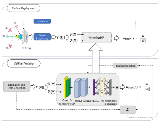
Figure 2: Systematic view of the proposed MambaBF approach, ”n” refer to the training sample.

To mitigate NGSOs’ CFI, we need a mechanism that can be trained offline to utilize any available $L$ snapshots of the array output $\mathbf{Y}$ and generate a robust weight vector $\mathbf{w}_{\text{MBF}}$ without prior knowledge of desired or interference channels. We propose a MambaBF to tackle this problem. Mamba-based SSMs layers were first introduced by [10] with the aim to address Transformers’ computational inefficiency on long sequences of the input data by allowing the parameters of the SSM to selectively retain or discard information along the sequence dimensions based on the current state (i.e., snapshots in our case), thus improving the model’s ability to handle sequences effectively.

III-A Model Overview

We aim at generating $\mathbf{w}_{\text{MBF}}$ directly from the received snapshots $\mathbf{Y}$ signal. Fig. 2 (lower panel) illustrates the offline training pipeline. When $L$ snapshots are collected, the data can be arranged in a matrix $\mathbf{Y}(n)\in\;\mathbb{C}^{M\times L},$ where $n$ is a training sample. Each complex entry is converted into its real and imaginary parts before being fed into the neural network, giving an input real-valued tensor of shape $(2M,L)$.

The real and imaginary parts of $\mathbf{Y}$ are first normalized and then processed by a 1D convolution (conv1D) plus max-pooling (MaxPool1D) across the snapshot dimension for dimensionality reduction. Each Conv1D output is Batch-normalized to stabilize training. After these initial layers, the latent input $\mathbf{x}\in\mathbb{R}^{M_{z}\times L}$, $M_{z}<2M$ is passed through the Mamba-based SSM layers (MmLs), followed by fully connected (FC) layers. The final output is a weight vector $\hat{\mathbf{w}}\in\mathbb{R}^{2M}$, reshaped into $\mathbb{C}^{M}$, then normalized to yield

$$\mathbf{w}_{\mathrm{MBF}}\;=\;\frac{\hat{\mathbf{w}}}{\|\hat{\mathbf{w}}\|}.$$ (14)

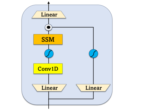
Figure 3: Mamba layer (MmL)

III-B Core Mamba Layer (MmL).

The structure of the Mamba layers (MmLs) [10] incorporates multi-modal feature extraction capabilities through the integration of linear transformations, convolutional operations, and recurrent sequence modeling. We enhance the local and global extraction of temporal and spatial features by stacking two Mamba layers. An MmL block handles sequences by merging two concurrent linear transformations of the input, as illustrated in Fig. 3. One pathway applies scaled exponential linear unit (SeLU) activation on the input,

$$\tilde{\mathbf{x}}(\ell)\;=\;\mathrm{SeLU}\bigl{(}\mathbf{x}(\ell))\bigr{)},$$ (15)

the other linear path is first processed by a conv1D with kernel size $k$, typically performing,

$$\mathbf{c}(\ell)\;=\;\mathrm{SeLU}\bigl{(}\mathrm{Conv1D}_{k}(\mathbf{x}(\ell))\bigr{)},$$ (16)

a Gated Recurrent Unit (GRU) further refines this sequence representation $\mathbf{c}(\ell)$ as a simple SSM model, as it unfolds over $\ell$ modeling long-term dependencies in the data,

$$\mathbf{g}(\ell)\;=\;\mathrm{GRU}\bigl{(}\mathbf{c}(\ell),\mathbf{g}(\ell-1)\bigr{)},$$ (17)

the output of the GRU is then element-wise multiplied with the skipped connection SeLU activation output, effectively acting as an attention-like mechanism to emphasize relevant features,

$$\mathbf{f}(\ell)\;=\;\mathbf{W}_{\mathrm{out}}\!\Bigl{(}\mathbf{g}(\ell)\,\odot\,\tilde{\mathbf{x}}(\ell)\Bigr{)},$$ (18)

where $\tilde{\mathbf{x}}(\ell)$ is a skip-connection transform of $\mathbf{x}(\ell)$, and $\odot$ denotes element-wise multiplication.

III-C Unsupervised Training Objective

The proposed learning procedure offers unsupervised training, and the loss function is customized to minimize $\mathcal{L}_{\mathrm{SINR}}(n)=-\mathrm{SINR}(n)$ in case of a single snapshot or minimize $\mathcal{L}_{\mathrm{ASINR}}(n)=-\frac{1}{L}\sum_{(n,l)}^{(n,L)}\mathrm{SINR}(l,n)$. Given $\mathbf{w}_{\mathrm{MBF}}(\mathbf{Y}(n))$, we measure $\mathcal{L}(n)$ in terms of the received power from the desired direction vs. interference plus noise. We then perform backpropagation through the MambaBF network using $\mathcal{L}(n+1)$ as our new cost.

IV Simulation Results

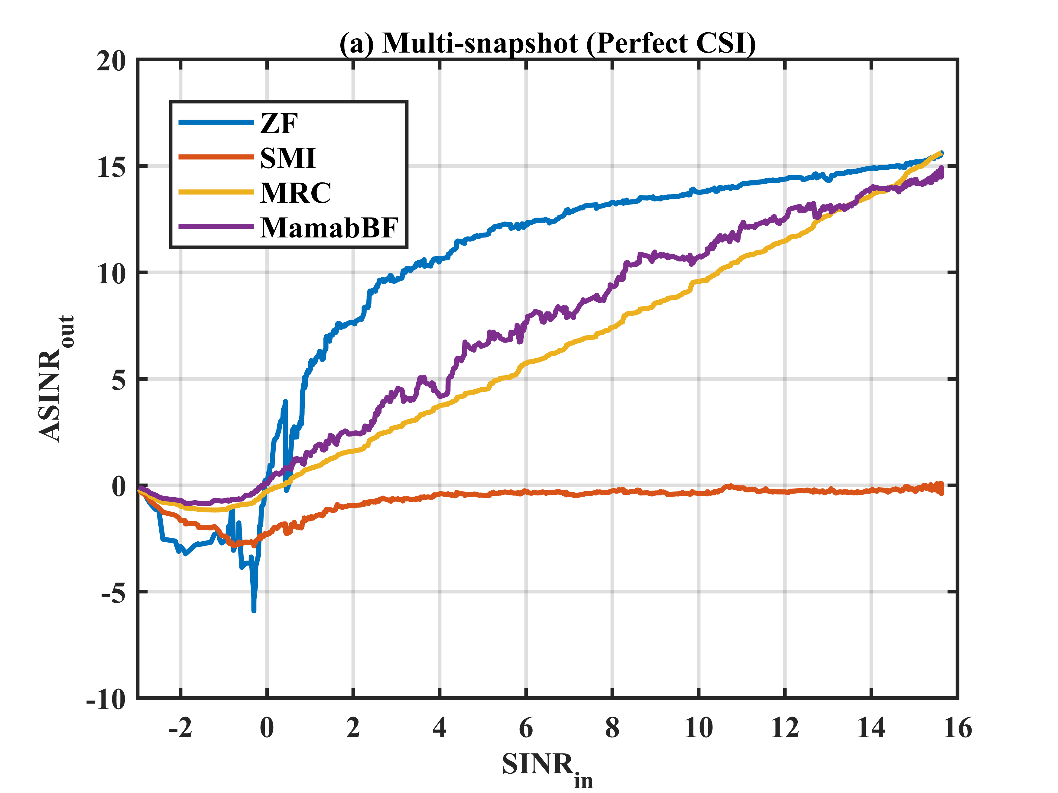
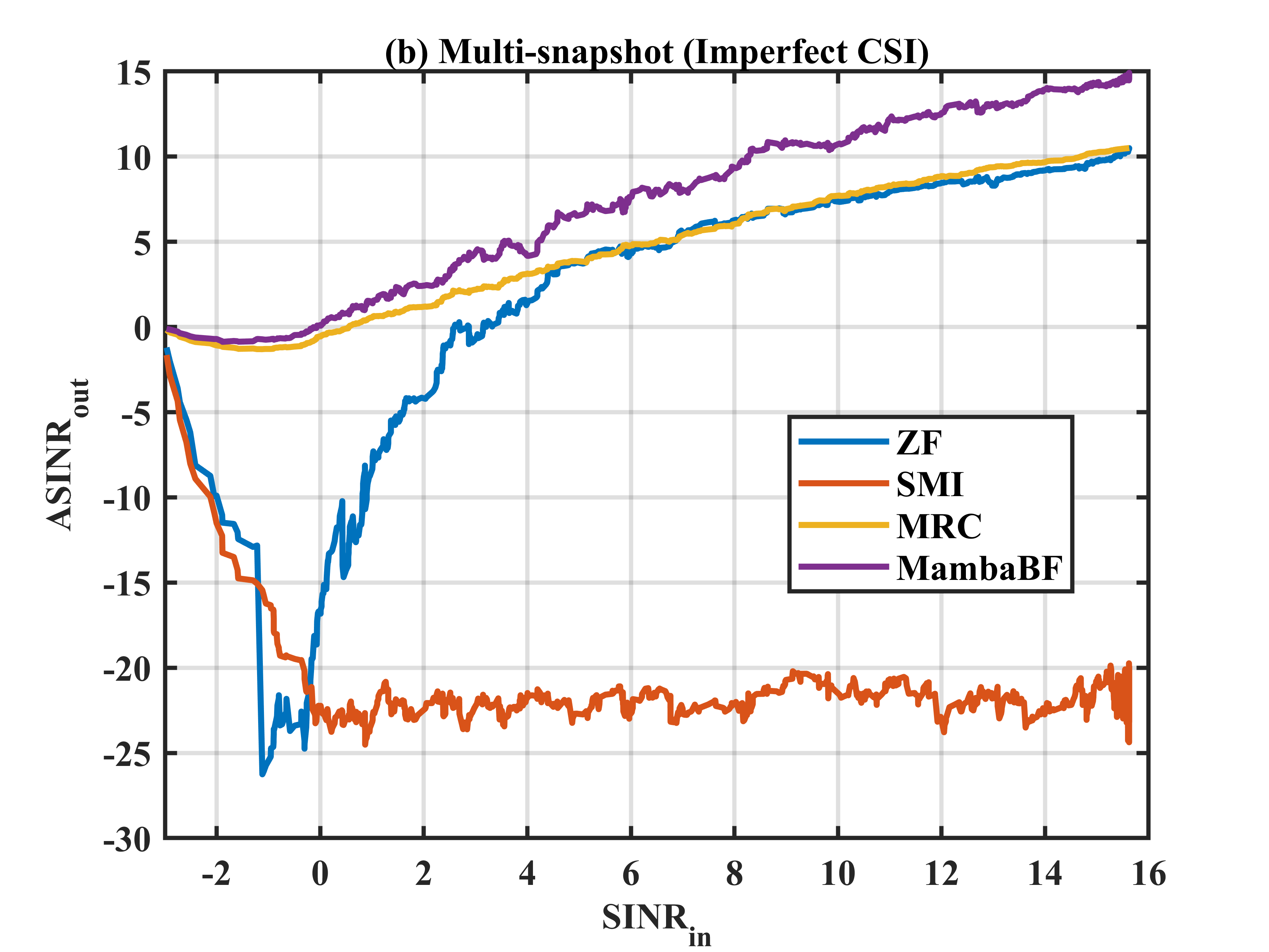
Figure 4: $\mathrm{ASINR}$ for multi-snapshot with (a) perfect CSI (left) and (b) imperfect CSI (right)

IV-A Parameters and Data Generation

Table I parameters were used to generate the interference scenarios in MATLAB, in addition to these parameters, the $\mathrm{DS}$ is assumed to have a pair of DOAs $\left[\phi_{d},\theta_{d}\right]=\left[0,0\right]$, while we assume $\mathrm{ISs}$ transmit severe interference (QoS degradation) could be around side lobe levels (SLLs), so for an array operating in scan angles $\phi,\theta\in\left[-90:90\right]$ the critical angles it is assumed to be $\phi_{k},\theta_{k}\in\left[-40:40\right]$. The UT directivity in (4) points at $\mathrm{DS}$ direction with efficiency $\eta^{ut}=0.99$ and $\mathbf{v}_{d}$ initial weights. This setup produces different $\mathrm{SINR}$ values, particularly low $\mathrm{SINR}$ at highly correlated desired and interference channels (in-line DOAs angles), and higher $\mathrm{SINR}$ values at less correlated channels or at nulled SLLs locations. We will train our models twice for two scenarios, when we have a single snapshot, and when we have multiple snapshots. The multi-snapshot data is generated at a sampling rate $f_{s}=2\times BW_{d}$ producing $200$ snapshots per training data sample ”$n$”, this is for the SMI benchmark where $\mathbf{\hat{R}}$ should be estimated assuming a full rank to ensure a good performance of the matrix inversion.

TABLE I: Scenarios Parameters

Parameters	Values
$M$	$10\times 10$ elements
$K$	3 satellites
$r_{d}$ , $r_{k}$	1000, $\left[500~\text{to}~600\right]$ Km
${P}_{d}$ , ${P}_{k}$	45 dBW, $40$ dBW
$f_{c,d}$ , $f_{c,i}$	11.750 GHz
$BW_{d}$ , $BW_{i}$	50 MHz
$\mathrm{DS}$ & $\mathrm{ISs}$ Modcods	QPSK, 8QAM
$T^{ut}$	230∘ K

To account for imperfect CSI, we introduce a 15% misalignment error (i.e., $\sigma_{e}^{2}=0.15)$ to the desired channel vector $\mathbf{h}_{d}$, while keeping the interference channel matrix $\mathbf{H}_{i}$ unaltered.

IV-B Model Training

The proposed model processes input tensors of shape $(\text{\text{Batch}},2M,L)$, where $\text{\text{Batch}}\leq[N_{\mathrm{tr}},N_{\mathrm{ts}}]$. We set $N_{\mathrm{tr}}=4000$ for training and $N_{\mathrm{ts}}=1000$ for testing. These samples are iteratively and randomly generated using the parameters in Section IV-A. Throughout the experiments, the Batch size is fixed to 16, and model weights are updated over 30 epochs. The model reduces the dimensionality of the input to $(\text{\text{Batch}},M_{z},L)$, where $M_{z}=100$.

IV-C Model Performance

We evaluate the performance of the proposed MambaBF beamformer using off-training (test) samples. Earlier, we assumed UPA has knowledge of the $\mathrm{DS}$’s DOA, thus the initial beamformer $\mathbf{w}_{\text{in}}$ is set to $\mathbf{v}_{d}(\varphi_{d})$. Our goal is to compare various beamformers’ performances by replacing $\mathbf{w}_{\text{in}}$ with a new updated beamformer $\mathbf{w}_{\text{out}}$ and measuring the resulting $\mathrm{SINR}_{\text{out}}(\mathbf{w}_{\text{out}})$ where $\mathbf{w}_{\text{out}}\in[\mathbf{w}_{\mathrm{ZF}},\mathbf{w}_{\mathrm{MRC}}$ $,\mathbf{w}_{\mathrm{SMI}},\mathbf{w}_{\mathrm{MBF}}]$.

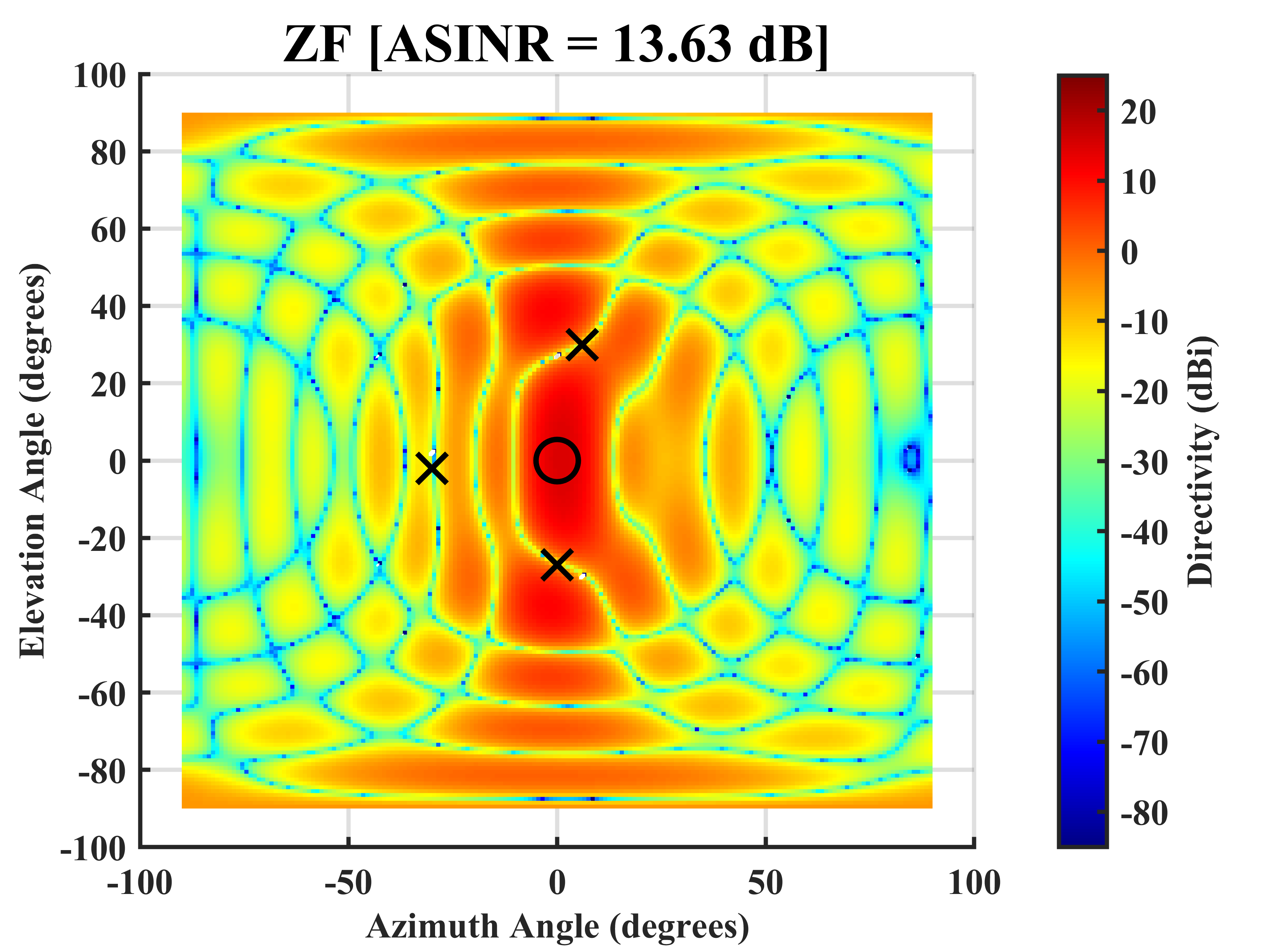
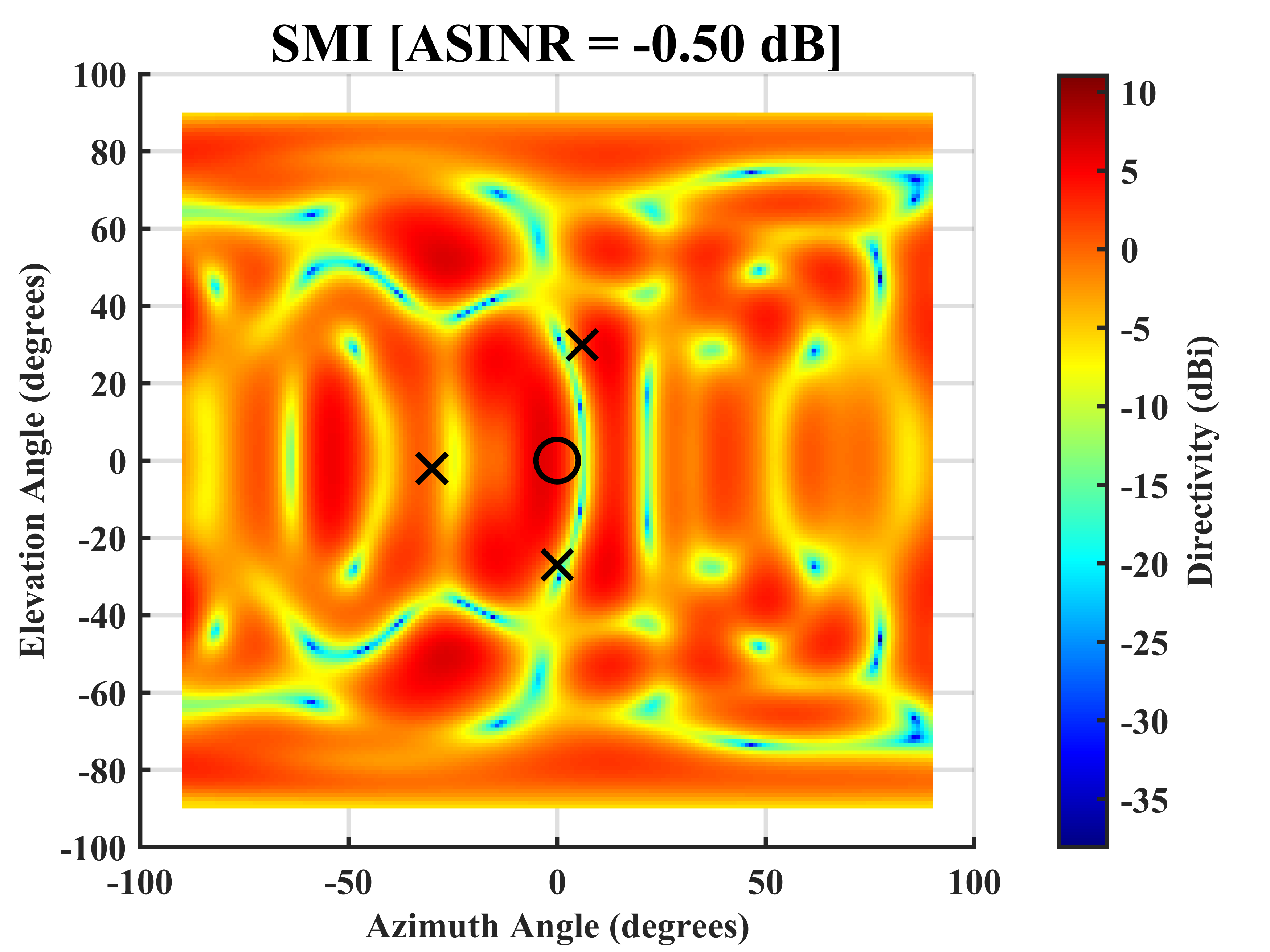
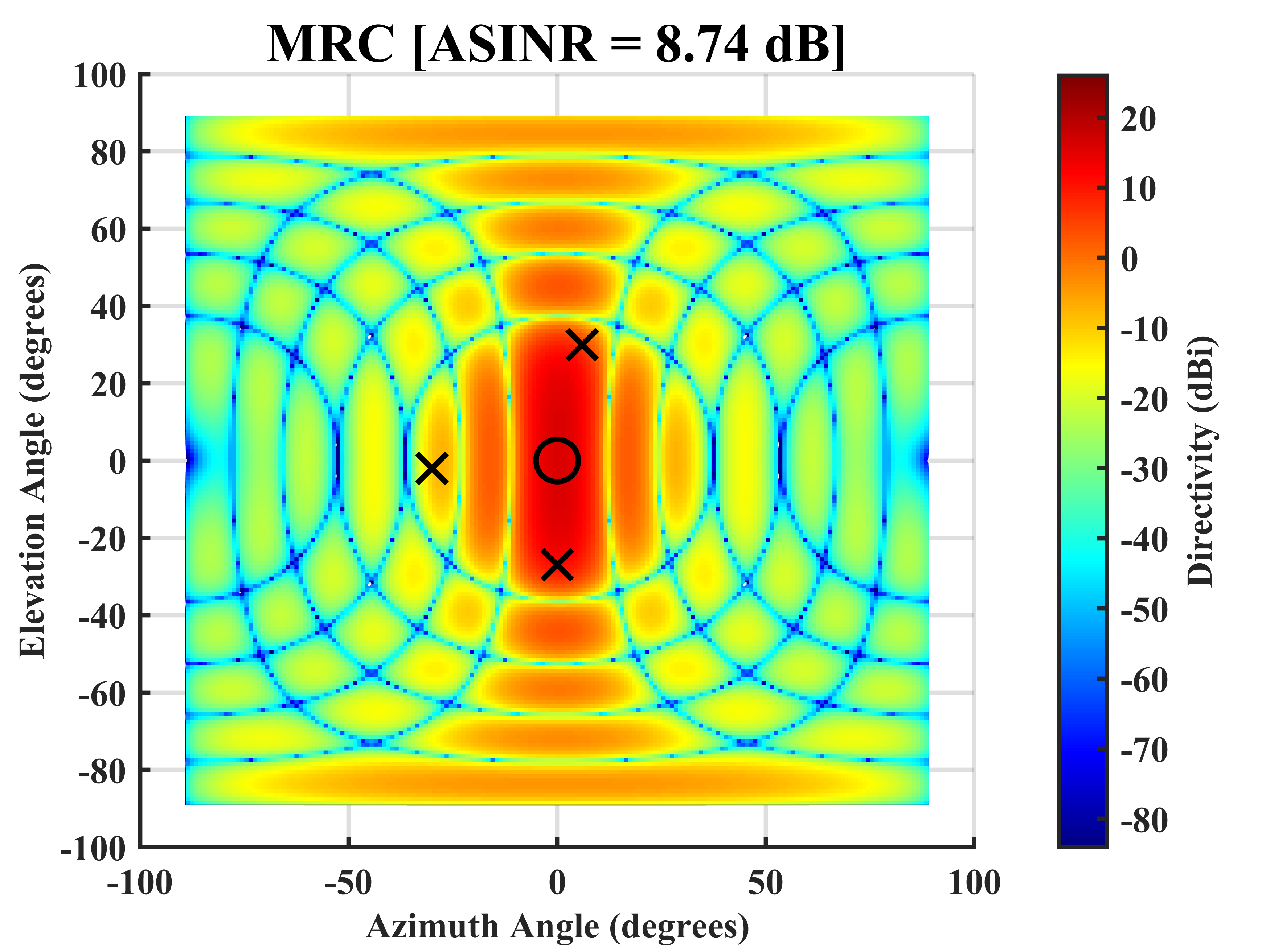
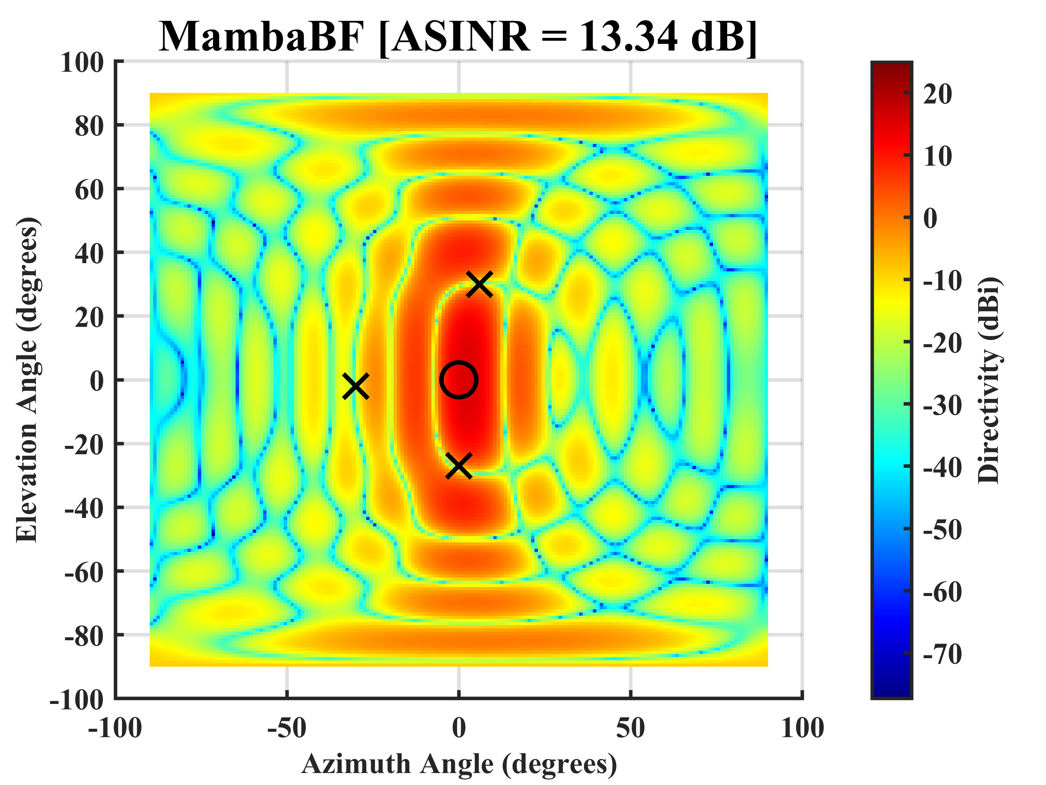
Figure 5: Beam nulling performance (representative case 1: perfect CSI)

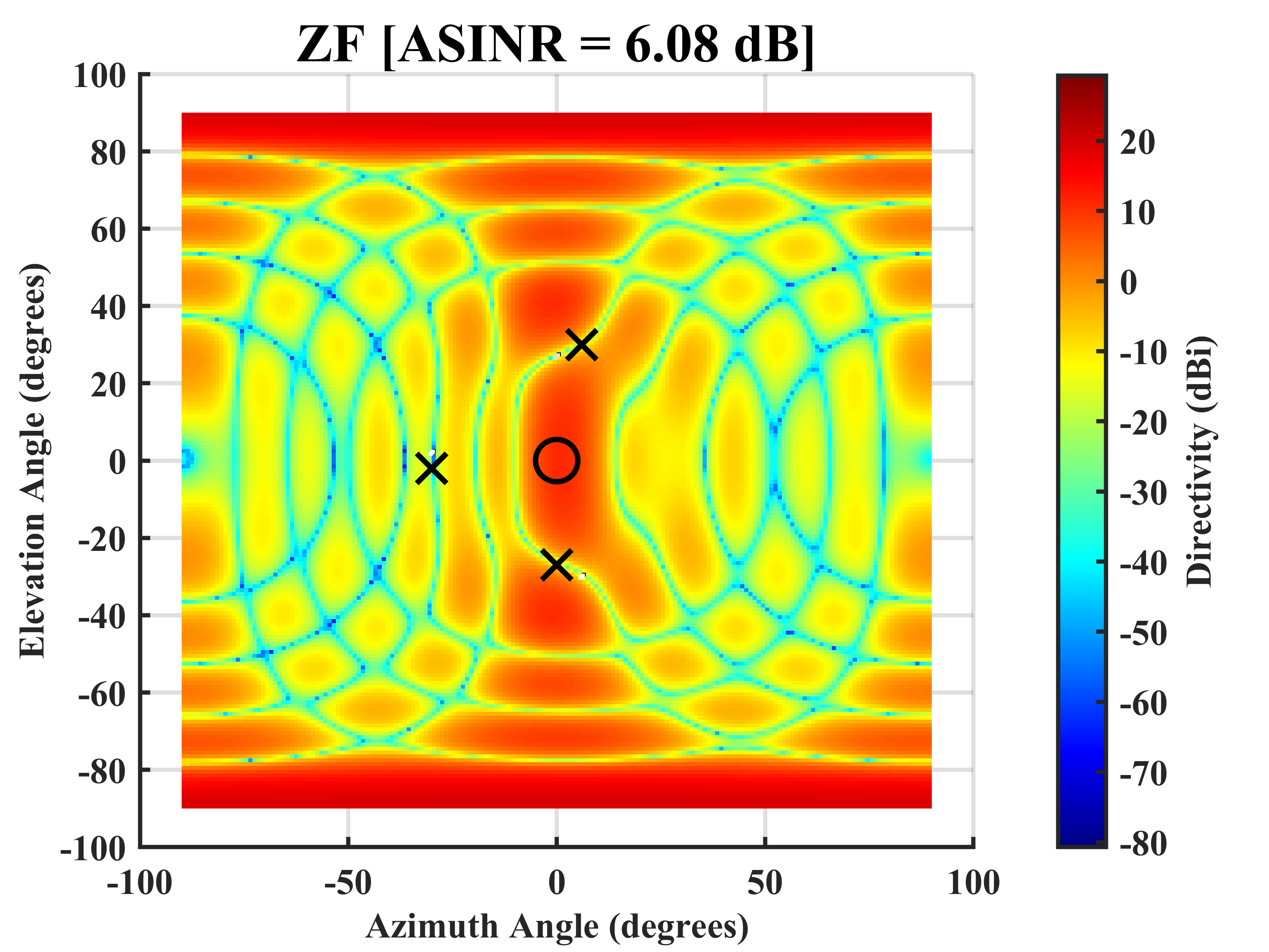
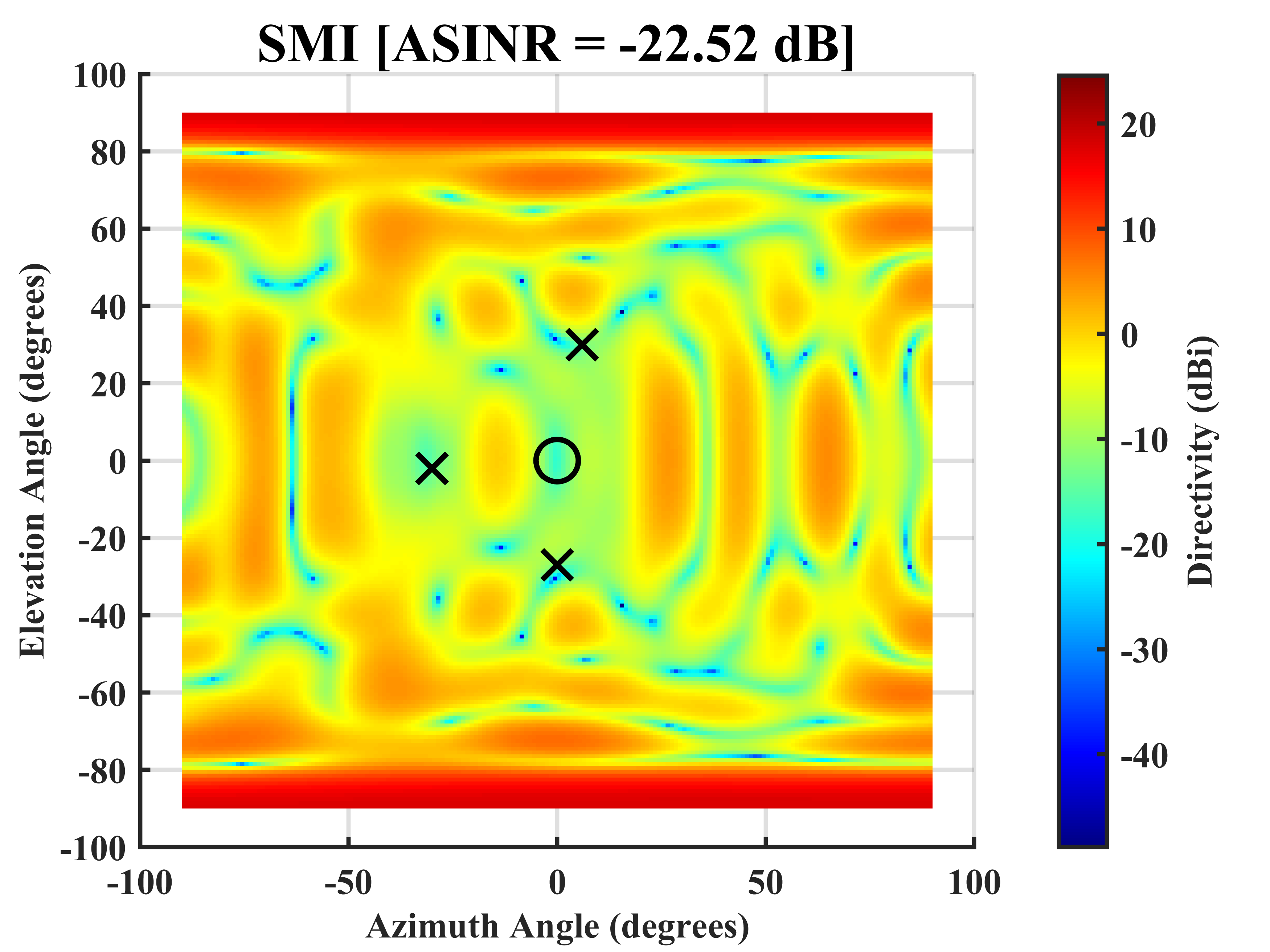
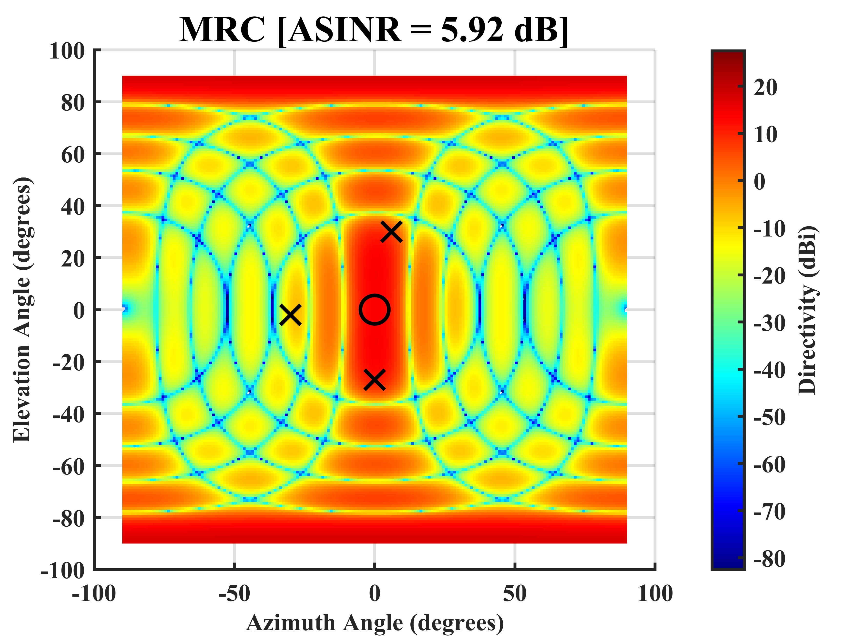
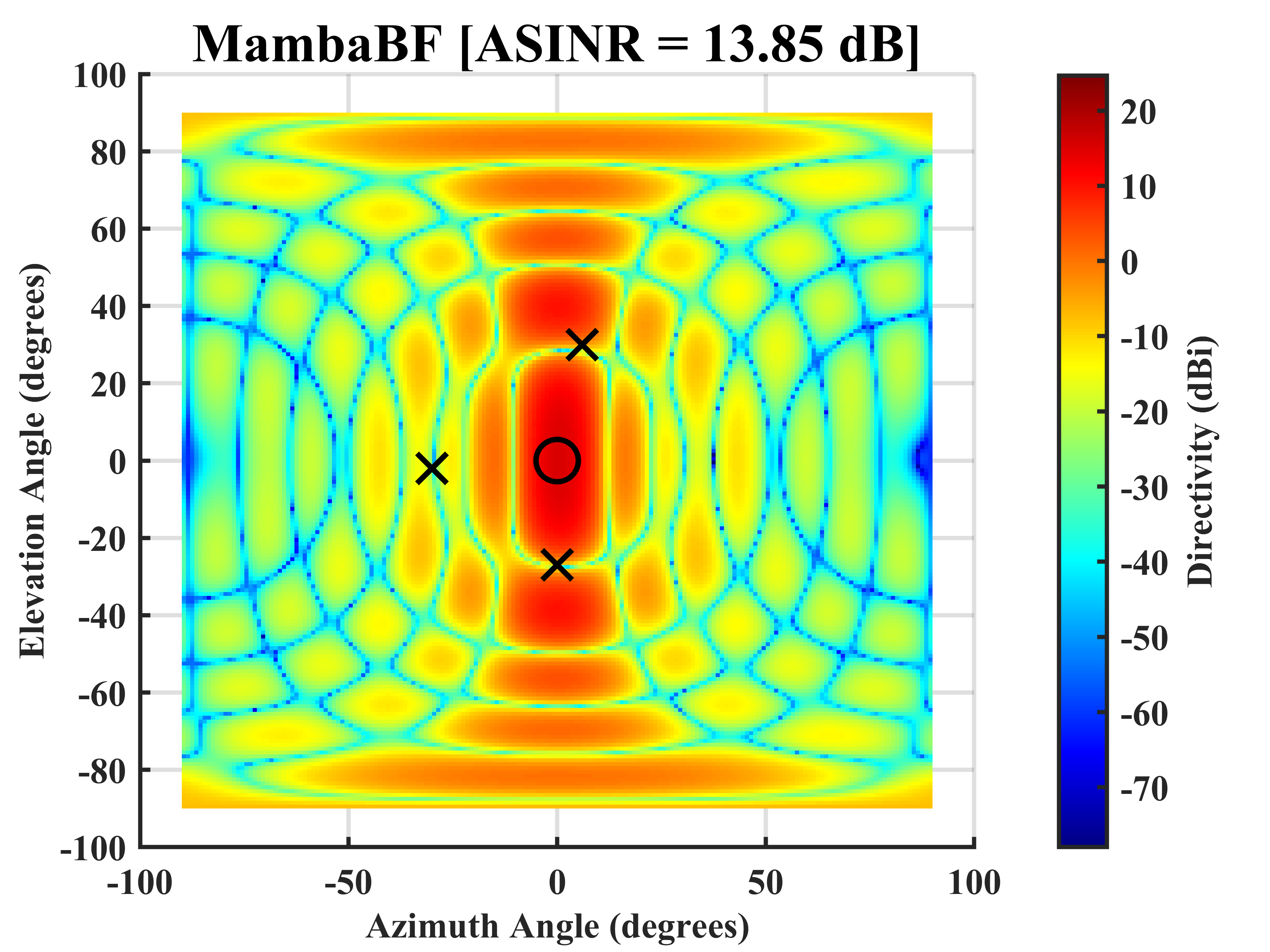
Figure 6: Beam nulling performance (representative case 2: imperfect CSI)

Figs. 4 plot $\mathrm{SINR}_{\mathrm{in}}$ versus $\mathrm{SINR}_{\mathrm{out}}$ for both perfect CSI and imperfect CSI conditions. a) Perfect CSI (Left Figure): SMI exhibits poor performance when the number of snapshots (here 200) is limited . ZF performs exceptionally well under high-quality CSI by exploiting full knowledge of the desired and interference channels; it fully cancels interference but struggles in negative $\mathrm{SINR}_{\mathrm{in}}$ due to the high correlation between desired and interference channels (i.e., $\mathbf{v}_{d}\approx\mathbf{v}_{k}$). MRC performs the worst among the classical approaches since it maximizes only the desired signal power without explicitly nulling interference. MambaBF consistently outperforms MRC and sometimes outperforms ZF at low $\mathrm{SINR}_{\mathrm{in}}$, converging at higher $\mathrm{SINR}_{\mathrm{in}}$ with minor fluctuations. b) Imperfect CSI (Right Figure): With channel estimation errors, SMI, ZF, and MRC see noticeable performance drops, illustrating their sensitivity to imperfect CSI. The MambaBF model, in contrast, outperforms these methods across both low and high $\mathrm{SINR}_{\mathrm{in}}$, showing robustness under realistic imperfect CSI conditions.

Figs. 5 and Figs. 6 illustrate a representative beam-nulling case under perfect and imperfect CSI conditions, respectively. Each sub-figure shows the array directivity (in dB) as a function of UT’s azimuth and elevation angles. The desired satellite’s DOA is marked with a black circle ($\circ$), while the interference satellite’s DOAs are indicated by black crosses ($\times$). The average output $\mathrm{SINR}$ ($\mathrm{ASINR}$) for each method is noted in square brackets. Due to the limited space, we cannot cover other cases. These figures show each approach performs at nulling interference locations, demonstrating the strengths and weaknesses of each beamforming approach. With accurate channel knowledge (Fig. 5), ZF effectively cancels the interference sources, achieving high $\mathrm{ASINR}$ at the cost of slightly reduced main-lobe gain in $\mathrm{DS}$ direction. SMI, by contrast, struggles to null both interference signals, leading to negative $\mathrm{ASINR}$ when the number of snapshots is insufficient. MRC maximizes the gain at $\mathrm{DS}$ direction, but does not suppress interference, resulting in a moderate $\mathrm{ASINR}$.

Notably, MambaBF demonstrates a balanced capability, its beam pattern is directed toward the $\mathrm{DS}$ while also trying to null the interferers, yielding an $\mathrm{ASINR}$ comparable to ZF but without requiring explicit CSI knowledge. Under channel estimation errors, ZF and MRC exhibit performance degradation relative to the perfect-CSI scenario. SMI is especially sensitive to imperfect covariance estimates, showing a pronounced drop in $\mathrm{ASINR}$. In contrast, MambaBF maintains robust interference nulling and $\mathrm{DS}$ gain enhancement, achieving the highest $\mathrm{ASINR}$ among the methods shown. Because MambaBF does not rely on explicit CSI, it adapts more effectively to channel misalignment errors, confirming its suitability for real-world applications where perfect CSI is rarely guaranteed.

V Conclusion and Future Work

We have presented MambaBF, an unsupervised DL beamforming method that maximizes the SINR and suppresses interference using only the available array snapshots, even with a single snapshot. Numerical results confirm that MambaBF is the most flexible approach, especially under imperfect CSI, where classical methods deteriorate. This highlights MambaBF’s potential for real-world deployments with inevitable channel imperfections. Potential future directions include evaluating MambaBF under more complex scenarios with moving users, as well as exploring larger-scale datasets for improving the beamforming capability to ZF (optimal) level performance.

References

- [1] H. Al-Hraishawi, H. Chougrani, S. Kisseleff, E. Lagunas, and S. Chatzinotas, “A survey on nongeostationary satellite systems: The communication perspective,” IEEE Communications Surveys & Tutorials, vol. 25, no. 1, pp. 101–132, 2023.
- [2] Y. He, Y. Li, and H. Yin, “Co-frequency interference analysis and avoidance between ngso constellations: Challenges, techniques, and trends,” China Communications, vol. 20, no. 7, pp. 1–14, 2023.
- [3] ITU, “Radio regulations,” ITU, Geneva, Switzerland, Tech. Rep., 2020.
- [4] C. Braun, A. M. Voicu, L. Simić, and P. Mähönen, “Should we worry about interference in emerging dense NGSO satellite constellations?” in 2019 IEEE International Symposium on Dynamic Spectrum Access Networks (DySPAN), 2019, pp. 1–10.
- [5] Starlink, “Setup guide,” https://api.starlink.com/public-files/installation_guide_standard_kit.pdf, (Accessed on 09/23/2024).
- [6] H. L. Van Trees, Optimum array processing: Part IV of detection, estimation, and modulation theory. John Wiley & Sons, 2002.
- [7] H. A. Kassir, Z. D. Zaharis, P. I. Lazaridis, N. V. Kantartzis, T. V. Yioultsis, and T. D. Xenos, “A review of the state of the art and future challenges of deep learning-based beamforming,” IEEE Access, vol. 10, pp. 80 869–80 882, 2022.
- [8] S. P. Shojaei, H. Soleimani, and M. Soleimani, “Supervised autoencoder-based beamforming approach for satellite mmwave communication,” International Journal of Antennas and Propagation, vol. 2024, no. 1, p. 6750409, 2024.
- [9] C. Vahapoglu, T. J. O’Shea, T. Roy, and S. Ulukus, “Deep learning based uplink multi-user simo beamforming design,” in 2024 IEEE International Conference on Machine Learning for Communication and Networking (ICMLCN), 2024, pp. 329–333.
- [10] A. Gu and T. Dao, “Mamba: Linear-time sequence modeling with selective state spaces,” in First Conference on Language Modeling, 2024. [Online]. Available: https://openreview.net/forum?id=tEYskw1VY2
- [11] O. E. Ayach, S. Rajagopal, S. Abu-Surra, Z. Pi, and R. W. Heath, “Spatially sparse precoding in millimeter wave MIMO systems,” IEEE Transactions on Wireless Communications, vol. 13, no. 3, pp. 1499–1513, 2014.
- [12] L. You, K.-X. Li, J. Wang, X. Gao, X.-G. Xia, and B. Ottersten, “Massive MIMO Transmission for LEO Satellite Communications,” IEEE Journal on Selected Areas in Communications, vol. 38, no. 8, pp. 1851–1865, 2020.
- [13] L. C. Godara, Smart Antennas. CRC Press, 2004.
- [14] A. B. Gershman, N. D. Sidiropoulos, S. Shahbazpanahi, M. Bengtsson, and B. Ottersten, “Convex optimization-based beamforming,” IEEE Signal Processing Magazine, vol. 27, no. 3, pp. 62–75, 2010.