A Likelihood Ratio Framework for Highly Motivated Subdominant Signals

Abstract

In particle physics and cosmology, distinguishing subtle new physics signals from established backgrounds is always a fundamental challenge for individual phenomenologists. This paper presents a simple and robust statistical framework to evaluate the compatibility of highly motivated (HM) theoretical models with the residual of the experimental results, focusing on scenarios where data appears consistent with background predictions. We develop a likelihood ratio test procedure that compares null and alternative hypotheses, emphasizing cases where new physics introduces small deviations from the background. We demonstrate the approach through two concrete examples, a localized excess and a modulation over an oscillatory background. We derive explicit conditions under which the effect of the background on the residual of the data must be accounted for. The framework’s practicality is highlighted and in addition to the limitation, strategies to simplify complex background modeling are discussed.

[first]organization=School of physics, Institute for Research in Fundamental Sciences (IPM),
postcode=P.O.Box 19395-5531, city=Tehran, country=Iran

1 Introduction

The outcomes of many experiments often do not lead to new discoveries but instead serve to confirm standard physics, collectively referred to as the background. However, motivated by various theoretical and experimental considerations, phenomenologists search for signs of new physics within these results. In many cases, the signal of new physics is expected to manifest as a subtle fluctuation over the well-understood background. In this regard, data visualization is an essential tool for researchers to interpret complex experimental results. Although, an over-reliance on visual representations can sometimes lead to misleading conclusions. This paper addresses two key issues arising from the visualization of results: a) the false identification of features in plots and b) the concealment of critical information that statistical analysis can reveal. The first issue is a topic frequently discussed in the literature, where random fluctuations or systematic effects can be exaggerated in visual interpretations, leading to the perception of false signals. This is one of the primary reasons why the 5$\sigma$ level of significance is required for discoveries in particle physics Junk and Lyons (2020). Conversely, we explore cases where weak or hidden signals, undetectable by eye, are uncovered through statistical tools. This is particularly important, as potential future discoveries may lie among phenomena with $\sim 2\sigma-3\sigma$ significance. Consequently, it is crucial to develop robust and straightforward procedures to study such scenarios, which are often considered as hints. As an example in Fowlie (2021), the need to develop criteria for identifying and highlighting potential anomalies is discussed.

Analyzing experimental results presents numerous challenges and requires careful consideration, demanding both skill and experience. For comprehensive yet brief reviews on statistics in particle physics, see Cousins (2018), while Lyons (2017) provides an insightful example of delicate but crucial details that require attention. However, researchers often need rapid yet reliable estimations to determine whether further investigation is warranted. This is more important when there is a theoretical motivation that supports our belief in the alternatives. As a result, for one seeking to evaluate the potential of new physics without delving deeply into complex analysis, the likelihood ratio test within the classical Frequentist hypothesis test serves as an excellent starting point. This is a well-established method that has been extensively studied (Cowan et al., 2011; Blennow et al., 2014). Nevertheless, robust statistical inference demands meticulous attention to detail. Key challenges include but not limited to accurately estimating the tail distributions of p-values to enhance precision Fowlie et al. (2022), properly accounting for effects such as the look-elsewhere (Davies, 1987; Ranucci, 2006; Gross and Vitells, 2010) and incorporating the systematic van Dyk and Lyons (2023). These considerations are essential for drawing ultimate conclusions from experimental data.

Hypothesis testing provide measure to compares the compatibility of two models with experimental data. These models are defined by the null hypothesis ($H_{0}$) and alternative ($H_{1}$) hypothesis, each with its own set of free parameters (for standard definitions, see Chap. 40 in Navas et al. (2024)). The null hypothesis $H_{0}$ represents a well-established model with strong empirical belief, while the alternative $H_{1}$ proposes a theoretically motivated but less constrained scenario. Crucially, we distinguish between “belief”, grounded in replicated experimental results and “motivation”, driven by anomalies in observations, theoretical extensions, or exploratory curiosity for detecting new phenomena in the future. To reflect this distinction, we label $H_{0}$ as Strongly Believed (SB) and $H_{1}$ as Highly Motivated (HM). Fig. 1 (upper panel) illustrates this with pseudo-data and appropriate predictions from an ideal SB and HM models, assuming Gaussian errors ($25\%$ of data). Here, we posit from prior motivations that new physics (if present) is an order of magnitude weaker than the background. The lower panel shows residuals from the $H_{0}$ prediction. We emphasize that $H_{1}$ risks overfitting unless it is truly HM—i.e., supported by theoretical arguments or experimental hints. In such cases, hypothesis testing remains a valuable tool for investigation.

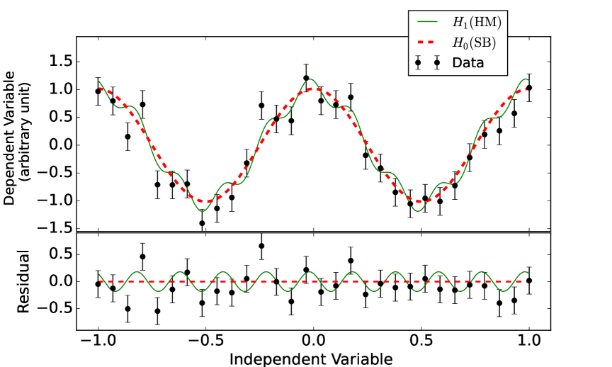
Figure 1: Upper panel: The pseudo-data are produced by considering a $25\%$ guassian noise to the true signal. line (dash-line) is the fit of $H_{0}$ ($H_{1}$) to data. Lower panel: residual of the data from $H_{0}$.

$H_{0}$ and $H_{1}$ are typically modeled with $P_{0}$ and $P_{1}$ free parameters, respectively. In many theories, $H_{0}$ is nested within $H_{1}$, meaning $H_{0}$ can be derived from $H_{1}$ by fixing $\tilde{P}_{1}$ parameters. Here, $\tilde{P}_{1}=P_{1}-P_{0}$ represents the number of additional parameters introduced by new physics. If $H_{1}$ includes parameters not shared with $H_{0}$ or beyond the $\tilde{P}_{1}$ constrained parameters, the look-elsewhere effect must be accounted for. In this study, we exclude such parameters. According to Wilks’ theorem Wilks (1938), for a sufficiently large sample size, the likelihood ratio test statistic $\lambda(x)$ under $H_{0}$ follows a chi-square distribution with $\tilde{P}_{1}$ degrees of freedom. In our example, $H_{1}$ introduces two additional parameters beyond $H_{0}$, so we expect $\lambda(x)$ to follow $\chi^{2}(2)$. Fig. (2) highlights the region where probability of finding the test larger than a critical value $\lambda_{c}$ equals to $P(\lambda(x)>\lambda_{c})=0.05$ and the values of $\lambda_{{\rm obs}}$ which is computed from the pseudo-data represented in Fig. (1) is determined inside this region. Choosing the p-value $\sim 0.05$ corresponds to the $\sim 2\sigma$ significance. It is deduced that this would be a hint for further investigation of an HM model. The next section details the derivation and interpretation of this test.

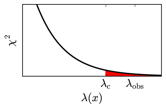
Figure 2: The distribution of test statistic $\lambda(x)$ for a model with two degrees of freedom. The values larger than $\lambda_{c}$ is highlighted. The result from data represented in Fig. (1) is determined by $\lambda_{\rm obs}$.

2 Likelihood Ratio Test

Let us assume we have $n$ independent data points $x=(x_{1},x_{2},\dots,x_{n})$, each labeled with $t=(t_{1},t_{2},\dots,t_{n})$, and the experiment provides error $\sigma=(\sigma_{1},\sigma_{2},\dots,\sigma_{n})$. Here, $x_{i}$ typically represents count-type measurements in high-energy physics, though they can also correspond to other types of measurements, while $t$ represents an independent variable such as energy or time. We assume that the data are Gaussian distributed. For count measurements, this is achieved by choosing a suitable number of bins.

Under the null hypothesis $H_{0}$, the observed data is predicted by the background showing with $b(t;\eta)$, where $\eta$ represents the free parameters of $H_{0}$. We are also interested in assessing the alternative hypothesis $H_{1}$, which explains the data using $\xi(t;\theta,\eta)$, where $\theta$ represents the free parameters associated with a new signal. Assuming $H_{0}$ is nested within $H_{1}$, the prediction of data under $H_{1}$ is given by:

$$\xi(t;\theta,\eta)=b(t;\eta)+\epsilon(t;\theta).$$ (1)

Our goal is to examine the new signal $\epsilon$ which represent itself as a fluctuation over the known background. $\epsilon$ could be represents a localized excess of events, bump or modulation in the background. Indeed we assume

$$\frac{\epsilon(t;\theta)}{b(t;\eta)}<O(0.1),$$ (2)

over the entire region of interest $t$ and for the relevant free parameters. This condition is common when searching for a new signal at the percent level in a measurement. Furthermore, we proceed our derivation with single parameter $\eta$ and $\theta$ for simplicity. Extension to more than one parameter is straightforward. To examine how the data prefer the new signal compare to the background we perform a standard hypothesis testing. To this end, first we derive the fit of background to data. Under the null hypothesis, as $\theta\to 0$, $\xi$ reduces to:

$$\xi(t;\eta)=b(t;\eta).$$ (3)

The chi-square statistic takes the form:

$$\chi^{2}_{0}(\eta)=\sum_{i}\frac{(x_{i}-b_{i}(\eta))^{2}}{\sigma_{i}^{2}},$$ (4)

where minimizing $\chi^{2}$ yields the best-fit value for the free parameter $\eta$, denoted as $\hat{\eta}$. Linearizing the background with respect to $\hat{\eta}$ (Fogli et al., 2002), we obtain:

$$b(t;\eta)=b(t;\hat{\eta})+\alpha(t)(\eta-\hat{\eta}).$$ (5)

Here, $\alpha(t)=\dfrac{\partial b(t;\hat{\eta})}{\partial\eta}$ is evaluated at $\hat{\eta}$, the best-fit value of $\eta$ under the null hypothesis $H_{0}$. It determines the scale of uncertainties at each bins to find new best fit values in presence of $\epsilon$. The $\hat{\eta}$ is determined by satisfying blew relation which is given by the minimization of Eq. (4) with respect to $\eta$

$$\sum_{i}\frac{\tilde{x}_{i}}{\sigma_{i}^{2}}\alpha_{i}=0,$$ (6)

where I define the residual of data by subtracting the trend as $\tilde{x}_{i}=x_{i}-b_{i}(\hat{\eta})$. Next, we turn to derive the estimator of free parameters under the alternative hypothesis. The chi-square statistic for the $H_{1}$ becomes:

$$\chi^{2}_{1}(\eta,\theta)=\sum_{i}\frac{\left(\tilde{x}_{i}-\alpha_{i}(\eta-\hat{\eta})-\epsilon_{i}(\theta)\right)^{2}}{\sigma_{i}^{2}}.$$ (7)

To minimize the chi-square under the alternative hypothesis $H_{1}$, we start with the partial derivative of $\chi^{2}$ with respect to $\eta$, given by:

$$\frac{\partial\chi^{2}_{1}}{\partial\eta}=-2\sum_{i}\frac{\left(\tilde{x}_{i}-\alpha_{i}(\eta-\hat{\eta})-\epsilon_{i}(\theta)\right)}{\sigma_{i}^{2}}\alpha_{i}=0.$$ (8)

Solving for $\eta$, taking to account the condition from Eq. (6) we find:

$$\eta_{\text{min}}(\theta)=\hat{\eta}-\dfrac{\sum_{i}\dfrac{\alpha_{i}\epsilon_{i}(\theta)}{\sigma_{i}^{2}}}{\sum_{i}\dfrac{\alpha_{i}^{2}}{\sigma_{i}^{2}}}$$ (9)

$\eta_{\text{min}}(\theta)$ represents the modified value of $\hat{\eta}$ in presence of new physics. It reveals that the shift from background-only estimation is encoded to the amount of correlation between fluctuation $\epsilon(t;\theta)$ and the $\alpha(t)$. To clarify this behavior, consider the idealized case where errors can be neglected. In the continuous limit, the second term in Eq. (7) reduces to:

$$\alpha(t)\left[\eta_{\text{min}}(\theta)-\hat{\eta}\right]=\alpha(t)\dfrac{\int\alpha(t)\epsilon(t;\theta)dt}{\int\alpha(t)^{2}dt},$$ (10)

where $\eta_{\text{min}}(\theta)$ represents the background parameter’s best-fit value for a given $\theta$. The impact of this term depends critically on the alignment between the signal model $\epsilon(t;\theta)$ and the background shape $\alpha(t)$: a) When $\epsilon(t;\theta)$ correlates strongly with $\alpha(t)$, the shift term is amplified, indicating significant background interference in the $\theta$ estimation. b) When $\epsilon(t;\theta)$ and $\alpha(t)$ are uncorrelated, the background’s influence on $\theta$ becomes negligible. We quantify this effect through the dimensionless shift parameter:

$$\rho(\theta)\equiv\dfrac{\langle\alpha(t)\epsilon(t;\theta)\rangle}{\langle\alpha(t)^{2}\rangle},$$ (11)

where $\langle\cdot\rangle$ denotes the weighted average over the independent variable $t$:

$$\langle f(t)\rangle\equiv\frac{\int f(t)/\sigma^{2}(t)dt}{\int 1/\sigma^{2}(t)dt}.$$ (12)

This parameter $\rho(\theta)$ directly measures the background-induced shift in the new physics parameter $\theta$.

Finally, to determine the best-fit value $\hat{\theta}$, we solve the partial derivative of $\chi^{2}$ with respect to $\theta$. Once both $\eta$ and $\theta$ are determined, the minimized $\chi^{2}$ under $H_{1}$ becomes:

$$\chi^{2}_{1}=\sum_{i}\frac{(\tilde{x}_{i}-\tilde{\epsilon}_{i})^{2}}{\sigma_{i}^{2}},$$ (13)

where $\tilde{\epsilon}_{i}$ represents the background-corrected predicted values:

$$\tilde{\epsilon}_{i}=\epsilon_{i}(\theta)-\alpha_{i}\rho(\theta).$$ (14)

For the special case of constant background where $\alpha_{i}$ is bin-independent, this simplifies to:

$$\tilde{\epsilon}_{i}=\epsilon_{i}(\theta)-\frac{\sum_{i}\epsilon_{i}(\theta)/\sigma_{i}^{2}}{\sum_{i}1/\sigma_{i}^{2}}\equiv\epsilon_{i}-\bar{\epsilon},$$ (15)

where $\bar{\epsilon}$ denotes the weighted average of the new physics. This implies that for constant background, one must: 1) First compute the residuals by subtracting the background, 2) Then set $\bar{\epsilon}=0$ by comparing $\epsilon_{i}-\bar{\epsilon}$ to the residuals.

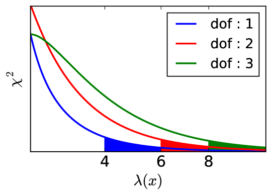
Figure 3: Distribution of test statistic $\lambda$ for different degrees of freedom. The essential values for the test to achieve more than $2\sigma$ significance is highlighted.

To distinguish between random fluctuations and genuine signals in the data, we employ the likelihood ratio test defined by:

$$\lambda=\chi^{2}_{\text{min},0}-\chi^{2}_{\text{min},1},$$ (16)

where $\chi^{2}_{\text{min},0}$ and $\chi^{2}_{\text{min},1}$ are the minimized $\chi^{2}$ values for the null and alternative hypotheses, respectively. By combining Eq. (4) and Eq. (13), we derive the test statistic:

$$\lambda(\tilde{x})=\sum_{i}\frac{\tilde{x}_{i}^{2}}{\sigma_{i}^{2}}-\sum_{i}\frac{(\tilde{x}_{i}-\tilde{\epsilon}_{i})^{2}}{\sigma_{i}^{2}},$$ (17)

where $\tilde{x}_{i}$ represents the observed data points and $\sigma_{i}$ their uncertainties. Under the null hypothesis, first term corresponds to the sum of squared noise contributions while $\lambda(\tilde{x})$ follows a $\chi^{2}$ distribution with degrees of freedom equal to the number of additional parameters $\theta$ in $H_{1}$ compared to $H_{0}$. To have an estimation of how the test indicate to new physics we find the $\lambda_{c}$ in such a way that the probability of finding $P(\lambda(\tilde{x})\geq\lambda_{c})\sim 0.05$ is satisfied:

$$\int_{\lambda_{c}}^{\infty}\chi^{2}(\tilde{P})d\lambda=0.05$$ (18)

The result of $\lambda_{\text{obs}}\leq\lambda_{c}$ is often considered as a hint for considering the signal model more seriously, investigate possible unknown systematic or presence of new physics. Fig. (3) shows the value of $\lambda_{c}$ satisfying $2\sigma$ significance for the case of 1, 2 and 3 degrees of freedom. In the following section, we illustrate this framework with two concrete examples.

3 Localized Excess

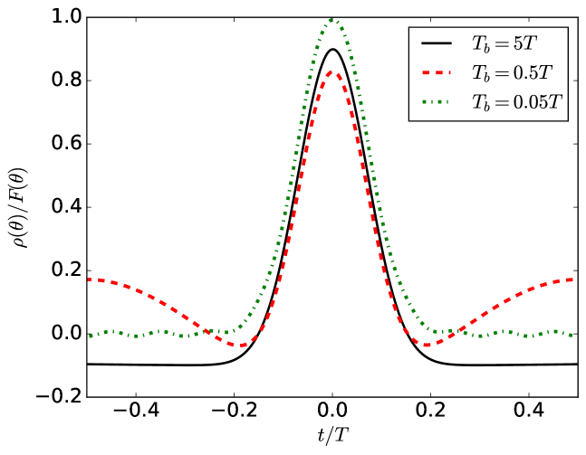
Figure 4: Effect of the background on the shape of the new signal when it is considered to predict the residual of the data for the case that new physics is suppose to be as a gaussian bump over an oscillatory background. The effect is modeled for three different oscillation.

To get more clear, I continue with an example. First example is a toy model that is applicable in many experiment in a more complex scheme. Consider a case where we are looking for a small bump in a specific location in a oscillatory background. The background is modeled by

$$b(t;\eta)=\eta f_{b}\cos(\dfrac{2\pi t}{T_{b}}).$$ (19)

For the simplicity we ignore initial phase set it to the zero at $t=0$. Following to previous section, $\eta$ is the dimension less free parameter of the null hypothesis and the period of the background is fixed to the $T_{b}$. The signal is modeled by a Gaussian function with unknown amplitude $\theta$

$$\epsilon(t;\theta,\sigma_{\epsilon})=\theta f_{\epsilon}e^{-\dfrac{(t-t_{0})^{2}}{\sigma_{\epsilon}^{2}}}.$$ (20)

The width of the excess we are looking for is determined by $\sigma_{\epsilon}$ and $\theta$ is the appropriate free parameter for new physics. Factor $f_{\epsilon}$ is present to regulate the dimension. $t_{0}$ is the location of the excess and it is assumed to be fixed. For the case when it is unknown we have to account for the look-elsewhere effect. From Eq. (10) we derive the shift term to account for the effect of background on the residual which is given by

$$\rho(\theta)=F(\theta)\dfrac{-2e^{-\left(\dfrac{\pi\sigma_{\epsilon}}{T}\right)^{2}}\cos(2\pi\frac{t_{0}}{T})}{1+\text{sinc}(2\pi T/T_{b})},$$ (21)

where $F(\theta)$ is the overall factor

$$\theta\frac{f_{\epsilon}}{f_{b}}\dfrac{\sigma_{\epsilon}\sqrt{\pi}}{\Delta t}.$$ (22)

times a constant coefficient. To derive Eq. (21) we assume the errors are constant. Furthermore we assume that it is in the limit $\sigma_{\epsilon}\ll T$, where the excess is localized in the small region inside the interval of the measurement is shown by $T$. The fraction $f_{\epsilon}/f_{b}$ must be small to ensure that the signal is appeared as a fluctuation in the background. For the $T_{b}\gg T\gg\sigma_{\epsilon}$ the background replace with a constant

$$b(t;\eta)=\eta f_{b}$$ (23)

and the modification of Eq. (21) reduce to

$$\rho(\theta)\approx-\theta\frac{f_{\epsilon}}{f_{b}}\dfrac{\sigma_{\epsilon}\sqrt{\pi}}{T},$$ (24)

where it is the average of the predicted excess as it is expected when the background behave as a constant. Therefore the new physics turn to

$$\tilde{\epsilon}(t;\theta,\sigma_{\epsilon})=\theta f_{\epsilon}\left(e^{-\frac{(t-t_{0})^{2}}{\sigma_{\epsilon}^{2}}}-\dfrac{\sigma_{\epsilon}\sqrt{\pi}}{T}\right).$$ (25)

In the limit of high oscillatory background $T\ll\sigma_{\epsilon}\ll T_{b}$ the exponential term in Eq. (21) damp the effect of background on the residual leading to

$$\tilde{\epsilon}(t;\theta,\sigma_{\epsilon})\approx\epsilon(t;\theta,\sigma_{\epsilon})$$ (26)

In the intermediate region $T_{b}\sim T$ additional bumps should be encountered which is famous as the alias effect. In Fig. (4) these cases are illustrated for $\sigma_{\epsilon}=0.05T$.

4 Modulation Excess

As a second example, we consider new physics modeled by an oscillatory behavior with a frequency distinct from the background. We parameterize the new physics contribution as:

$$\epsilon(t;\theta,\phi)=\theta f_{\epsilon}\cos\left(\frac{2\pi t}{T_{\epsilon}}+\phi\right),$$ (27)

where, similar to the previous example, $T_{\epsilon}$ is assumed to be known. For cases with unknown frequency, the look-elsewhere effect must be incorporated in the hypothesis tests. Here, $f_{\epsilon}$ carries the appropriate physical dimensions, while $\theta$ and $\phi$ are dimensionless free parameters.

Using Eq. (10), the modification term takes the form:

$$\rho(\theta,\phi)=F(\theta,\phi)\dfrac{\text{sinc}(2\pi T/T_{+})+\text{sinc}(2\pi T/T_{-})}{1+\text{sinc}(2\pi T/T_{b})},$$ (28)

where the amplitude factor $F(\theta,\phi)$ is given by:

$$F(\theta,\phi)=\theta\cos(\phi)\frac{f_{\epsilon}}{f_{b}},$$ (29)

and the characteristic periods $T_{\pm}$ are defined as:

$$\frac{2}{T_{\pm}}=\frac{1}{T}\pm\frac{1}{T_{\epsilon}}.$$ (30)

The factor $F(\theta,\phi)$ reveals important physical regime. When the phase difference $\phi$ between signal and background approaches $\pi/2$, the shift term vanishes due to the $\cos(\phi)$ dependence. In the limit of large frequency separation ($T_{b}\ll T_{\epsilon}$ or $T_{b}\gg T_{\epsilon}$), the coefficient tends to zero. However, when the new signal’s frequency and phase align closely with the background, the shift term $\rho$ becomes enhanced and exhibits degeneracy with the new physics parameters. This degeneracy complicates the parameter extraction and requires careful analysis.

5 Summary and conclusions

In this study, we have focused on experimental results consistent with background predictions, which has been very common in recent years, while acknowledging the existence of highly motivated (HM) theories that require empirical constraints. The presented procedure offers a simple and efficient approach to evaluate the compatibility of alternative hypotheses with data compares to the background model, instead of relying on the visually inspection of plots. Our framework is applicable when the following conditions are satisfied:

1. The alternative hypothesis $H_{1}$ must be HM to minimize overfitting risks.

2. The new physics contribution should be at least one order of magnitude smaller than the background, satisfying $\epsilon(t,\theta)/b(t,\eta)\leq\mathcal{O}(0.1)$. This condition is typically met since we do not expect new physics to dramatically violate established physics.

3. Background uncertainties should be well-controlled, not exceeding $\sim 10\%$, a requirement often achieved in experiments with percent-level precision.

While our analysis employs a simplified background model, actual experimental scenarios involve complex background sources from multiple contributions. To address this complexity while maintaining practicality, we recommend:

• Utilizing experimental residuals when they are available

• Focusing on specific data regions where new physics may contribute

• Modeling background derivatives by fitting simple functions to the final total experimental background estimates provided by collaborations

Several important limitations warrant careful consideration:

• In cases where the bins are not Gaussian or where the distribution of the test statistic does not follow the chi-square distribution due to experimental limitations, one has to use a modified version of Eq. (13) and determine the distribution of the test statistic through numerical simulations

• Inter-bin correlations often manifest as correlated errors that must be accounted for. Reader can find for example a precise study on the “pull” approach to including the correlated errors Fogli et al. (2002).

• The test is not expected to yield highly significant ($4\sigma-5\sigma$) results, as we fundamentally assume background consistency at first order

• Results in the $2\sigma-3\sigma$ range may indicate potential hints, but they require careful assessment of possible unknown systematics

• While not discussed here, calculating the power of the test (typically denoted by $\beta$) could provide valuable insights for such scenarios. The power calculation follows a similar procedure to the hypothesis test, requiring only an estimation of the distribution of $\lambda(\tilde{x})$ under the $H_{1}$ hypothesis, which can be obtained through numerical approaches (See for example Navas et al. (2024)).

After examining these considerations, we emphasize that any detected hints can be particularly valuable for future experiment planning. Moreover, in cases showing null compatibility, the same framework can be applied to put constrain on new physics parameters, following procedures well-documented in the literature.

References

- Blennow et al. (2014) Blennow, M., Coloma, P., Huber, P., Schwetz, T., 2014. Quantifying the sensitivity of oscillation experiments to the neutrino mass ordering. JHEP 03, 028. doi:10.1007/JHEP03(2014)028, arXiv:1311.1822.
- Cousins (2018) Cousins, R.D., 2018. Lectures on Statistics in Theory: Prelude to Statistics in Practice arXiv:1807.05996.
- Cowan et al. (2011) Cowan, G., Cranmer, K., Gross, E., Vitells, O., 2011. Asymptotic formulae for likelihood-based tests of new physics. Eur. Phys. J. C 71, 1554. doi:10.1140/epjc/s10052-011-1554-0, arXiv:1007.1727. [Erratum: Eur.Phys.J.C 73, 2501 (2013)].
- Davies (1987) Davies, R.B., 1987. Hypothesis testing when a nuisance parameter is present only under the alternative. Biometrika 74, 33–43. doi:10.1093/biomet/74.1.33.
- van Dyk and Lyons (2023) van Dyk, D., Lyons, L., 2023. How to Incorporate Systematic Effects into Parameter Determination arXiv:2306.05271.
- Fogli et al. (2002) Fogli, G.L., Lisi, E., Marrone, A., Montanino, D., Palazzo, A., 2002. Getting the most from the statistical analysis of solar neutrino oscillations. Phys. Rev. D 66, 053010. doi:10.1103/PhysRevD.66.053010, arXiv:hep-ph/0206162.
- Fowlie (2021) Fowlie, A., 2021. Comment on ”Reproducibility and Replication of Experimental Particle Physics Results” doi:10.1162/99608f92.b9bfc518, arXiv:2105.03082.
- Fowlie et al. (2022) Fowlie, A., Hoof, S., Handley, W., 2022. Nested Sampling for Frequentist Computation: Fast Estimation of Small p-Values. Phys. Rev. Lett. 128, 021801. doi:10.1103/PhysRevLett.128.021801, arXiv:2105.13923.
- Gross and Vitells (2010) Gross, E., Vitells, O., 2010. Trial factors for the look elsewhere effect in high energy physics. Eur. Phys. J. C 70, 525–530. doi:10.1140/epjc/s10052-010-1470-8, arXiv:1005.1891.
- Junk and Lyons (2020) Junk, T.R., Lyons, L., 2020. Reproducibility and Replication of Experimental Particle Physics Results doi:10.1162/99608f92.250f995b, arXiv:2009.06864.
- Lyons (2017) Lyons, L., 2017. A Paradox about Likelihood Ratios? arXiv:1711.00775.
- Navas et al. (2024) Navas, S., et al. (Particle Data Group), 2024. Review of particle physics. Phys. Rev. D 110, 030001. doi:10.1103/PhysRevD.110.030001.
- Ranucci (2006) Ranucci, G., 2006. Likelihood scan of the Super-Kamiokande I time series data. Phys. Rev. D 73, 103003. doi:10.1103/PhysRevD.73.103003, arXiv:hep-ph/0511026.
- Wilks (1938) Wilks, S.S., 1938. The Large-Sample Distribution of the Likelihood Ratio for Testing Composite Hypotheses. Annals Math. Statist. 9, 60–62. doi:10.1214/aoms/1177732360.