Feedback-Driven Pseudo-Label Reliability Assessment: Redefining Thresholding for Semi-Supervised Semantic Segmentation

Abstract

Semi-supervised learning leverages unlabeled data to enhance model performance, addressing the limitations of fully supervised approaches. Among its strategies, pseudo-supervision has proven highly effective, typically relying on one or multiple teacher networks to refine pseudo-labels before training a student network. A common practice in pseudo-supervision is filtering pseudo-labels based on pre-defined confidence thresholds or entropy. However, selecting optimal thresholds requires large labeled datasets, which are often scarce in real-world semi-supervised scenarios. To overcome this challenge, we propose Ensemble-of-Confidence Reinforcement (ENCORE), a dynamic feedback-driven thresholding strategy for pseudo-label selection. Instead of relying on static confidence thresholds, ENCORE estimates class-wise true-positive confidence within the unlabeled dataset and continuously adjusts thresholds based on the model’s response to different levels of pseudo-label filtering. This feedback-driven mechanism ensures the retention of informative pseudo-labels while filtering unreliable ones, enhancing model training without manual threshold tuning. Our method seamlessly integrates into existing pseudo-supervision frameworks and significantly improves segmentation performance, particularly in data-scarce conditions. Extensive experiments demonstrate that integrating ENCORE with existing pseudo-supervision frameworks enhances performance across multiple datasets and network architectures, validating its effectiveness in semi-supervised learning.

1 Introduction

Supervised deep learning has demonstrated remarkable success in computer vision tasks, often surpassing classical machine learning methods. However, this success is contingent on large-scale annotated datasets, which are costly and time-intensive to obtain. Semantic segmentation, in particular, demands extensive pixel-wise annotations, making it significantly more expensive than region- or image-level annotation [26]. Even state-of-the-art segmentation networks [4, 5, 51, 55, 29, 17] suffer from performance degradation in low-data regimes. The challenge is even more pronounced in medical image segmentation, where annotations require domain expertise and are highly labor-intensive.

To mitigate this reliance on labeled data, semi-supervised learning (SSL) has gained traction by leveraging large amounts of unlabeled data to improve generalization and domain adaptability [54, 6, 19, 25, 24]. Among SSL techniques, pseudo-labeling is a widely adopted strategy in semantic segmentation [23], where a model trained on labeled data generates approximate ground-truth labels for unlabeled images, incorporating them into training.

Pseudo-supervision methods typically employ a pretrained network [47], a mean teacher [37], or multiple teacher models [30, 52, 9] to enhance pseudo-labeling. To mitigate error propagation, pseudo-labels undergo a filtering stage to exclude low-confidence predictions. However, existing confidence-based filtering approaches face limitations: high-confidence thresholds (e.g., 0.95) risk discarding numerous correct pseudo-labels, while hyperparameter search for threshold tuning contradicts the real-world constraints of SSL, where labeled data is scarce and a sufficiently large validation set is impractical.

Moreover, in low-data regimes, model performance is highly sensitive to the choice of confidence threshold, yet this dependency follows no consistent pattern (see Figure 1). As labeled dataset size decreases, the optimal threshold becomes increasingly unpredictable, significantly affecting segmentation performance. A fixed threshold may be too strict, discarding useful pseudo-labels, or too lenient, introducing noisy predictions. This issue is exacerbated by inter-class variability in confidence levels, where different classes exhibit varying prediction certainty, further complicating threshold optimization.

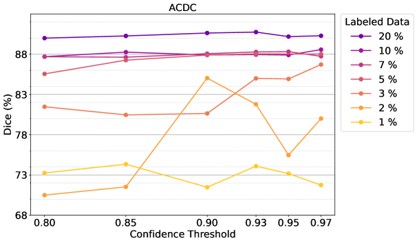
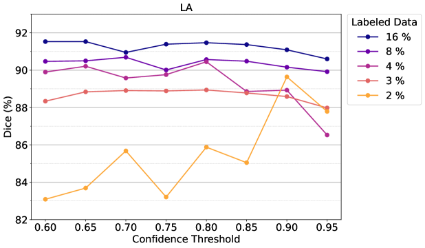
Figure 1: Comparison of Dice scores across different confidence thresholds for various labeled data percentages on the ACDC and LA datasets with AD-MT [52]. The plots illustrate how segmentation performance fluctuates with threshold selection, particularly in low-data regimes. As the labeled data fraction decreases, model sensitivity to threshold choice increases, making optimal threshold selection more challenging. Notably, a fixed global threshold often fails to generalize well across different dataset conditions, underscoring the need for an adaptive thresholding strategy.

To address these challenges, we propose Ensemble-of-Confidence Reinforcement (ENCORE), a two-stage pseudo-label assessment strategy that integrates Class-Aware Confidence Calibration (CAC) and Adaptive Confidence Thresholding (ACT). CAC estimates class-wise pseudo-label confidence using only the available labeled dataset, ensuring that pseudo-label filtering accounts for inter-class confidence variability. ACT then dynamically adjusts confidence thresholds throughout training based on real-time feedback, eliminating the need for manual threshold tuning. Specifically, our contributions are as follows:

• We introduce Class-Aware Confidence Calibration (CAC), which computes class-wise confidence thresholds by estimating the model’s average true-positive confidence per class. This accounts for class-dependent variability in prediction confidence, ensuring more reliable pseudo-label selection. Accordingly, we utilize CAC to initialize class-wise pseudo-label filtering thresholds without requiring additional validation data or hyperparameter tuning.

• We propose Adaptive Confidence Thresholding (ACT), a dynamic threshold adjustment mechanism that continuously refines pseudo-label filtering during training. ACT evaluates the student model’s response to different thresholds using labeled batches and iteratively selects the most effective threshold for each stage of training.

• Our fully automated thresholding strategy, implemented within ENCORE, eliminates a major hyperparameter in pseudo-supervision while significantly enhancing semi-supervised learning performance across different pseudo-labeling frameworks.

The remainder of this paper is structured as follows: Section 2 reviews recent advancements in semi-supervised semantic segmentation. Section 3 details our proposed framework, Ensemble of Confidence Reinforcement (ENCORE). The experimental setup is described in Section 4, followed by experimental results and analysis in Section 5. Finally, Section 6 summarizes our findings and discusses future research directions.

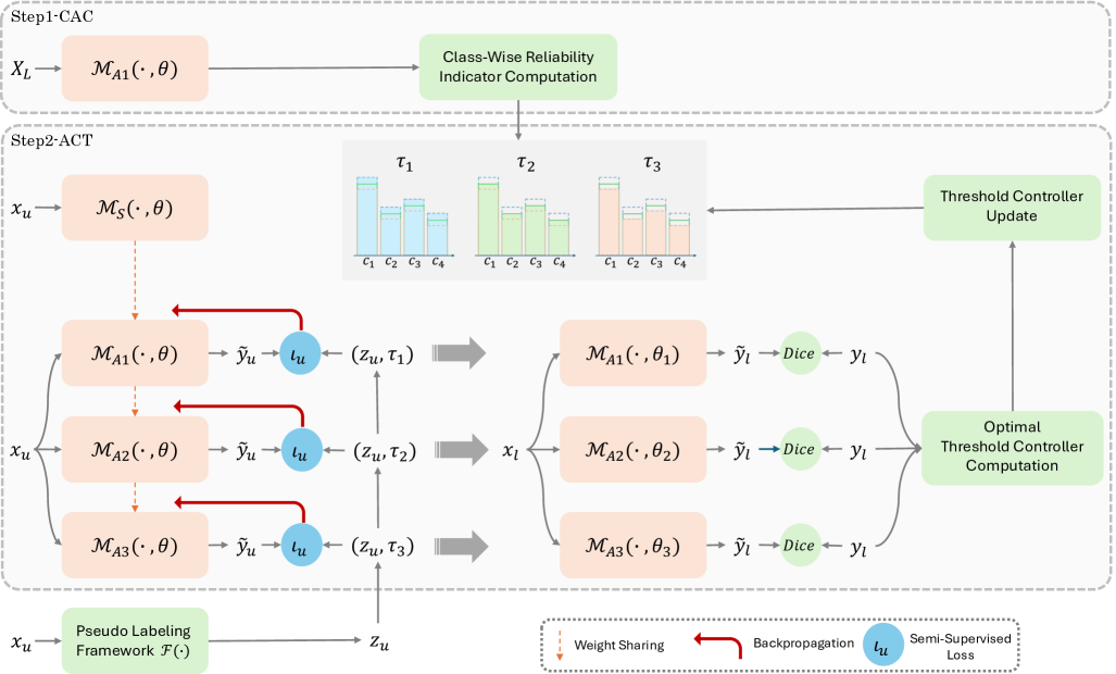
Figure 2: Overview of ENCORE: A feedback-driven pseudo-label refinement framework integrating Class-Aware Confidence Calibration (CAC) and Adaptive Confidence Thresholding (ACT) to enhance pseudo-label reliability and improve semi-supervised segmentation.

2 Related work

Semi-Supervised Learning (SSL) aims to enhance model performance while minimizing annotation efforts by leveraging unlabeled data during training. SSL approaches can be broadly categorized into three paradigms: (i) contrastive learning, (ii) consistency regularization [37, 40, 22, 33, 35, 28, 20, 21, 32], and (iii) pseudo-supervision [56, 25, 57, 7, 8, 13, 38, 49, 31, 12, 47, 42, 15, 18, 11].

Contrastive Learning focuses on robust representation learning. This technique enhances SSL by maximizing the similarity between related data instances while minimizing it for unrelated ones, improving feature consistency [18, 53, 39, 41]. By enforcing high agreement among similar samples and low agreement among dissimilar pairs, contrastive learning effectively captures the underlying structure of the input data, further improving segmentation performance in SSL frameworks.

Consistency regularization enforces stable model predictions under different conditions, ensuring robustness against variations such as (a) input perturbations, including data transformations [34, 45, 21, 30, 52, 48], (b) network perturbations, such as stochastic initializations [28], and (c) latent space augmentations [28] and drop-out [48]. Additionally, temporal consistency strategies enforce stability across different training checkpoints, reducing prediction variance [22].

Pseudo-Supervision enhances SSL by expanding the training set using model-generated pseudo-labels for unlabeled data. This method follows three primary paradigms: self-training, co-training, and mean teacher models. Self-training relies on a model to generate pseudo-labels for unlabeled samples, retaining only high-confidence predictions for subsequent training [47, 57, 44, 56, 15, 49, 36]. In contrast, co-training employs multiple models trained on different data perspectives, where each model generates pseudo-labels to iteratively improve the other’s predictions [7, 11], enhancing robustness and generalization.

Pseudo-supervision methods primarily focus on three challenges: 1) Improving pseudo-label reliability, 2) Mitigating confirmation bias, which arises when incorrect pseudo-labels reinforce model errors, and 3) Adapting pseudo-label incorporation strategies to improve model generalization, particularly in low-data regimes.

3 Method

In this section, we formally define the problem and introduce our proposed thresholding framework for semi-supervised semantic segmentation. We begin with a mathematical formulation of the problem, followed by an overview of the proposed approach. Subsequently, we provide a detailed explanation of its two key components in Sec. 3.1 and Sec. 3.2.

Problem Definition. We consider a labeled dataset $\mathcal{D^{L}}=\{(x_{l}^{i},y_{l}^{i})\}_{i=1}^{N^{\mathcal{L}}}$, consisting of training images $\mathcal{X}$ and their corresponding segmentation labels $\mathcal{Y}$, as well as an unlabeled dataset $\mathcal{D^{U}}=\{x_{u}^{i}\}_{i=1}^{N^{\mathcal{U}}}$, containing only the unlabeled image set $\mathcal{U}$, where $N^{\mathcal{U}}\gg N^{\mathcal{L}}$. Our objective is to train a model $\mathcal{M}_{S}(\cdot,\theta)$ that leverages both labeled and unlabeled data to improve segmentation performance on unseen samples. To achieve this, we adopt a semi-supervised learning paradigm, where pseudo-labels are assigned to the images in $\mathcal{U}$ using a pseudo-supervision framework. The overall training objective is defined as $\mathcal{L}_{\text{overall}}=\mathcal{L}_{l}+\lambda\mathcal{L}_{u}$, where $\mathcal{L}_{l}$ is the supervised loss on labeled data, $\mathcal{L}_{u}$ is the unsupervised loss on pseudo-labeled data, and $\lambda$ is a framework-dependent weighting hyperparameter that balances the contribution of the two terms. The core challenge is to identify and filter out unreliable pseudo-labels when computing $\mathcal{L}_{u}$ to maximize segmentation performance.

Overview. Figure 2 illustrates the framework of our proposed semi-supervised semantic segmentation method, termed ‘‘Ensemble-of-Confidence Reinforcement" (ENCORE). The method introduces a feedback-driven, adaptive thresholding framework that improves pseudo-label reliability. The student network ($\mathcal{M}_{S}(\cdot,\theta)$) learns from both labeled and pseudo-labeled data, while a set of assessor networks ($\{\mathcal{M}_{Ai}(\cdot,\theta_{i})\}_{i=1}^{3}$) dynamically evaluate pseudo-label reliability based on feedback derived from the student’s response to labeled images. At the core of our approach are two key innovations: Class-Aware Confidence Calibration (CAC) and Adaptive Confidence Thresholding (ACT). CAC refines pseudo-label selection by computing class-wise reliability scores, ensuring that confidence thresholds are adjusted per class rather than relying on a static global threshold. ACT further improves pseudo-label selection by iteratively evaluating different threshold levels using assessor networks and selecting the optimal threshold based on segmentation performance on labeled data. Unlike conventional methods with fixed confidence thresholds, ENCORE continuously adapts its thresholding strategy based on real-time feedback, preventing over- or under-filtering of pseudo-labels and enhancing segmentation accuracy. By integrating CAC and ACT, our approach dynamically calibrates confidence levels and optimally selects pseudo-labels, leading to more reliable supervision and improved segmentation performance.

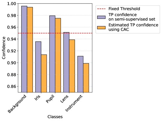
Figure 3: Comparison between CAC-based confidence thresholds and fixed thresholds for Cataract-1K dataset (1/8 labeled data).

3.1 Class-Aware Confidence Calibration (CAC)

Standard pseudo-label confidence indicators, such as the maximal softmax probability, often suffer from calibration issues, leading to suboptimal pseudo-label selection. Conventional methods like UniMatch [30, 52, 9, 48, 37, 43, 28] apply a single, global confidence threshold $\tau$ uniformly across all classes. However, this one-size-fits-all approach fails to account for class-specific score distributions. As a result, setting $\tau$ too high disproportionately filters out correct pseudo-labels for inherently low-confidence classes, increasing false negatives. Conversely, lowering $\tau$ to accommodate these classes introduces excessive false positives for high-confidence classes. This highlights a critical limitation: a fixed confidence threshold fails to capture class-wise prediction reliability, motivating the need for a more adaptive, class-sensitive confidence measure.

To address this issue, we propose Class-Aware Confidence Calibration (CAC), which estimates prediction reliability on a per-class basis. CAC utilizes the labeled training set as a reference to assess how model confidence correlates with ground-truth correctness for each class. Instead of applying a uniform threshold, CAC dynamically determines class-specific confidence levels by computing the average confidence of true positive detections (Figure 3).

Formally, let $\mathcal{Y}=\{y_{l}^{i}\}_{i=1}^{N^{\mathcal{L}}}$ denote the ground-truth labels, and let $\mathcal{M}_{A}(\mathcal{X})=\{\mathcal{M}_{A}(x_{l}^{i})\}_{i=1}^{N^{\mathcal{L}}}$ represent the network outputs for the labeled images. The predicted label for each image is then given by:

$$\hat{y}_{l}^{i}=\arg\max_{C}\Big{(}\tilde{y}_{l}^{i}\Big{)},$$ (1)

where $\tilde{y}_{l}^{i}\in\mathbb{R}^{C\times W\times H}$ represents the softmax probabilities across all classes, defined as $\tilde{y}_{l}^{i}=\sigma\big{(}\mathcal{M_{A}}(x_{l}^{i})\big{)}$, with $\sigma$ being the softmax operator. The class-wise reliability indicator $R$ is then computed as:

$$R =[R_{1},R_{2},.,R_{C}],$$ (2)

$$R_{c\in\{1,C\}} =\frac{1}{N^{\mathcal{L}}}\sum_{i=1}^{N^{\mathcal{L}}}\frac{1}{N_{i}^{c}}\sum_{j=1}^{k}\Big{(}[\hat{y}_{l}^{ij}=c]\times[y_{l}^{ij}=c]\Big{)},$$

$$N_{i}^{c} =\sum_{j=1}^{k}[y_{l}^{ij}=c],$$

where $C$ is the number of classes, $k$ represents the number of pixels in the segmentation mask $y_{l}$, and $[P]$ denotes the Iverson bracket, which evaluates to 1 if $P$ is true and 0 otherwise.

The class-wise reliability indicator $R$ is computed once using a network trained solely on labeled images and is set as the initial class-wise confidence threshold in the first iteration of semi-supervised learning. This enables a more adaptive pseudo-label selection strategy, ensuring that confidence thresholds are class-specific rather than globally fixed, thereby reducing bias toward high-confidence classes and improving segmentation performance across all classes.

3.2 Adaptive Confidence Thresholding (ACT)

While the CAC module mitigates inter-class confidence variability, it does not inherently ensure that filtering pseudo-labels based on the reliability indicator maximizes segmentation performance. The optimal balance between bridging the distribution gap and minimizing false positives depends on various factors, including dataset characteristics, the fraction of labeled data, the network’s training progression (e.g., epoch number), and the underlying semi-supervised framework. Instead of relying on a fixed class-wise confidence threshold, we propose an adaptive threshold selection strategy that evaluates multiple threshold levels, compares their performance, and dynamically selects the most suitable one. To achieve this, we initialize three class-wise confidence threshold controllers as follows:

$$(\tau_{1},\tau_{2},\tau_{3})=(\alpha_{1}R,R,\alpha_{2}R),$$ (3)

where $R$ represents the class-wise reliability indicator computed via CAC, and $\alpha_{1},\alpha_{2}$ are threshold adaptors that define the initial search space.

At each iteration, three assessor networks are instantiated by copying the current student model weights. Each assessor network applies a different threshold controller to filter pseudo-labels before training on the pseudo-labeled batch. The segmentation performance of each assessor is then evaluated on the labeled batch using the Dice metric, and the threshold controller that yields the highest Dice score is selected as the optimal controller for pseudo-label filtering in the next student model training cycle:

$$\tau^{*}=\operatorname*{argmax}_{\tau_{k}\in\{\tau_{1},\tau_{2},\tau_{3}\}}\text{Dice}(\mathcal{M}_{A_{k}}(x_{l};\theta_{k}),y_{l},\tau_{k}),$$ (4)

where $\mathcal{M}_{A_{k}}$ denotes the assessor network trained with threshold $\tau_{k}$, and $\text{Dice}(\cdot,\cdot,\tau_{k})$ evaluates segmentation performance with threshold $\tau_{k}$.

As training progresses, the recurrent selection of a particular threshold controller provides insight into whether the confidence thresholds should be dynamically adjusted. If the lowest or highest confidence threshold is consistently chosen, this suggests that the model’s overall confidence levels should be shifted downward or upward, respectively. The threshold controllers are updated according to:

$$(\tau_{1},\tau_{2},\tau_{3})=\begin{cases}(\alpha_{1}\tau_{1},\tau_{1},\alpha_{2}\tau_{1}),&\text{if }\tau^{*}=\tau_{1}\text{ and }N_{\tau^{*}}\geq n,\\ (\alpha_{1}\tau_{3},\tau_{3},\alpha_{2}\tau_{3}),&\text{if }\tau^{*}=\tau_{3}\text{ and }N_{\tau^{*}}\geq n,\\ (\tau_{1},\tau_{2},\tau_{3}),&\text{else}.\end{cases}$$ (5)

Here, $\alpha_{1}$ and $\alpha_{2}$ determine how aggressively the confidence thresholds are adjusted. To prevent excessive adaptation, we introduce a mechanism that modifies the threshold controllers only if the same threshold controller is selected more than $n$ consecutive times. Hence, $N_{\tau^{*}}$ tracks the number of consecutive selections of $\tau^{*}$.

Although $\alpha_{1}$ and $\alpha_{2}$ are fixed hyperparameters, our dynamic feedback-driven adaptation eliminates manual tuning by iteratively refining confidence thresholds based on model performance. This metric-adaptive calibration ensures that pseudo-labels meet robustness criteria—such as the Dice metric—enhancing segmentation accuracy based on observed performance rather than predefined heuristics.

This approach adaptively refines threshold controllers, allowing the model to dynamically adjust confidence filtering in response to its learning progression, improving pseudo-label reliability throughout training.

Input :

Labeled training set $\mathcal{D^{L}}=\{(x_{l}^{i},y_{l}^{i})\}_{i=1}^{N^{\mathcal{L}}}$,

Unlabeled training set $\mathcal{D^{U}}=\{(x_{u}^{i})\}_{i=1}^{N^{\mathcal{U}}}$,

Student model $\mathcal{M}_{S}(\cdot,\theta)$,

Pseudo-labeling framework $\mathcal{F}(\cdot)$,

Assessor models $\mathcal{M}_{A1}$, $\mathcal{M}_{A2}$, $\mathcal{M}_{A3}$,

Output :

Trained student model $\mathcal{M}_{S}(\cdot,\theta)$.

Train an assessor network on labeled images.

Compute the class-wise reliability indicator. $\triangleright$ Eq. (2)

Initialize confidence threshold controllers. $\triangleright$ Eq. (3)

for each mini-batch pair in ($\mathcal{D^{L}}$, $\mathcal{D^{U}}$) do

2     Compute pseudo labels for the unlabeled training batch $\tilde{y}_{u}$=$\mathcal{F}(x_{u})$, Load the assessor models with the current student weights. Train the assessor models on $x_{u}$ using the threshold controllers. Compute the optimal threshold controller. $\triangleright$ Eq. (4) Train the student model with optimal threshold controller. Update threshold controllers. $\triangleright$ Eq. (5)

3 end for

Algorithm 1 Ensemble-of-Confidence Reinforcement for Semi-Supervised Semantic Segmentation

4 Experimental setup

Dataset.

We evaluate the proposed and baseline methods on five widely used benchmarks for medical image segmentation from different modalities:

• Cataract-1K dataset [14], which consists of the annotations of the eye’s relevant anatomical objects including iris, pupil, intraocular lens, plus instruments in 2256 frames out of 30 cataract surgery videos. For semi-supervised settings, we randomly select six cases as the test set, $[13,6,3,1]$ cases (corresponding to $[1/2,1/4,1/8,1/16]$ splits) out of the training set as the supervised set, and the remaining cases will be used as the unlabeled semi-supervised set.

• Prostate MRI dataset [27] includes 116 prostate MRI volumes from six different sites. For each fold, 16 volumes are randomly sampled as the test set, and $[1/2,1/4,1/8,1/14,1/25,1/50]$ of the cases are randomly sampled as the labeled set.

• EndoVis dataset [1] includes annotations of instruments from 73 endoscopic surgery videos. We split these videos in a patient-wise manner to the training and testing set. Afterward, the training set is split into supervised and semi-supervised sets, with the rate of supervised images being equal to $[1/2,1/4,1/8,1/16,1/32,1/64,1/128]$.

• ACDC dataset [3], which includes 100 cine-MRI scans consisting of four classes (background, right ventricle, left ventricle, and myocardium). For this dataset, we adhere to all the settings outlined in [52], while excluding it from our configurations. The training set is splited into different volumes at ratios of $[1/7,1/14,1/70,1/140]$, corresponding to 262, 136, 26, and 13 slices, respectively.

• LA dataset [46], which comprises 100 3D late gadolinium-enhanced (LGE) MR scans with corresponding left atrium segmentation mask. In accordance with the task settings described in [52], we partitioned the dataset into 80 training scans—with volume splits of $[1/10,1/20,1/26,1/40]$— and 20 testing scans, applying identical preprocessing procedures across the board.

Implementation Details.

For LCDC and LA datasets, we follow all settings of AD-MT [52]. Specifically, we use UNet for ACDC and VNet for LA dataset. For remaining datasets, we utilize DeepLabV3+ [5] with a ResNet50 backbones [16] initialized with the ImageNet [10] pre-trained parameters. Besides, the network includes dropout layers in the decoder. For fair comparisons, the hyperparameters are maintained the same for all semi-supervised methods. We use stochastic gradient descent for optimization. The initial learning rate ($lr_{init}$) of the randomly-initialized segmentation head is set to 0.005 for Cataract-1K, and 0.001 for other datasets. The learning rate of the pre-trained encoder is $10\%$ of that of the segmentation head. The learning rate is decreased during training using polynomial decay with the power of 0.9: $lr=lr_{init}\times(1-\frac{iter}{total-iter})$. All models are trained for 80 epochs on the Cataract-1K and 40 epochs on Prostate MRI and EndoVis datasets. For the loss function, we adhere to the loss formulation specified by each semi-supervised framework. As weak augmentations, all images are randomly rescaled, horizontally flipped with the probability of $0.5$, and cropped with a size of $(384,384)$ for Cataract-1K, $(352,256)$ for EndoVis, and $(256,256)$ for other datasets. The strong augmentations include color-jittering (with an intensity factor of 0.6 for brightness and contrast, and 0.4 for saturation), and a random selection of Gaussian blur and random-adjust-sharpness. Besides, $(\alpha_{1},\alpha_{2})=(0.98,1.02)$ and $n$ is set to five iterations across all settings.

Alternative methods.

We compare the performance of the proposed method with state-of-the-art semi-supervised learning frameworks including Mean Teacher [37], CPS [7], RL [50], ST++ [47], PS-MT [28], MCF [43], BCP [2], UniMatch [48], Switch [30], GPS [9], and AD-MT [52].

Evaluation.

For all scenarios except ACDC and LA datasets, we employ a four-fold validation approach and present the averaged results across all folds. We evaluate the performance of all methods using the dice coefficient. All experiments are conducted on ‘‘NVIDIA RTX: 3090" GPUs. To support reproducibility, the training splits for all datasets and codes will be released with the acceptance of the paper.

5 Experimental Results

Table 1: Comparisons with state-of-the-art methods on Cataract-1K test set (Network: DeepLabV3+) based on dice coefficient ($\%$).

Framework		1/2 (987)	1/4 (433)	1/8 (242)	1/26 (61)	Rel. Avg.
Supervised		$87.85\;{\color[rgb]{.5,.5,.5}\pm 0.3}$	$82.55\;{\color[rgb]{.5,.5,.5}\pm 1.9}$	$76.72\;{\color[rgb]{.5,.5,.5}\pm 2.2}$	$60.34\;{\color[rgb]{.5,.5,.5}\pm 3.9}$	N/A
MT[37]	[NeurIPS 2017]	$87.10\;{\color[rgb]{.5,.5,.5}\pm 1.0}$	$85.59\;{\color[rgb]{.5,.5,.5}\pm 1.8}$	$84.57\;{\color[rgb]{.5,.5,.5}\pm 0.7}$	$73.47\;{\color[rgb]{.5,.5,.5}\pm 2.0}$	5.82
CPS [7]	[CVPR 2021]	$89.68\;{\color[rgb]{.5,.5,.5}\pm 6.7}$	$84.77\;{\color[rgb]{.5,.5,.5}\pm 6.6}$	$79.89\;{\color[rgb]{.5,.5,.5}\pm 6.2}$	$64.63\;{\color[rgb]{.5,.5,.5}\pm 8.2}$	2.88
RL [50]	[MICCAI 2021]	$85.74\;{\color[rgb]{.5,.5,.5}\pm 1.2}$	$84.78\;{\color[rgb]{.5,.5,.5}\pm 1.0}$	$83.33\;{\color[rgb]{.5,.5,.5}\pm 0.5}$	$74.66\;{\color[rgb]{.5,.5,.5}\pm 1.3}$	5.26
ST++ [47]	[CVPR 2022]	$88.73\;{\color[rgb]{.5,.5,.5}\pm 0.2}$	$84.32\;{\color[rgb]{.5,.5,.5}\pm 1.0}$	$80.74\;{\color[rgb]{.5,.5,.5}\pm 0.9}$	$64.57\;{\color[rgb]{.5,.5,.5}\pm 2.3}$	2.73
PS-MT [28]	[CVPR 2022]	$89.09\;{\color[rgb]{.5,.5,.5}\pm 4.1}$	$86.44\;{\color[rgb]{.5,.5,.5}\pm 4.7}$	$83.02\;{\color[rgb]{.5,.5,.5}\pm 6.7}$	$62.94\;{\color[rgb]{.5,.5,.5}\pm 7.3}$	3.51
MCF [43]	[CVPR 2023]	$89.21\;{\color[rgb]{.5,.5,.5}\pm 7.3}$	$84.44\;{\color[rgb]{.5,.5,.5}\pm 4.1}$	$79.57\;{\color[rgb]{.5,.5,.5}\pm 1.6}$	$66.62\;{\color[rgb]{.5,.5,.5}\pm 3.9}$	3.10
BCP [2]	[CVPR 2023]	$87.23\;{\color[rgb]{.5,.5,.5}\pm 0.3}$	$86.11\;{\color[rgb]{.5,.5,.5}\pm 1.1}$	$81.86\;{\color[rgb]{.5,.5,.5}\pm 1.9}$	$72.32\;{\color[rgb]{.5,.5,.5}\pm 2.0}$	5.01
GPS [9]	[WACV 2024]	$89.48\;{\color[rgb]{.5,.5,.5}\pm 0.5}$	$86.67\;{\color[rgb]{.5,.5,.5}\pm 1.1}$	$81.24\;{\color[rgb]{.5,.5,.5}\pm 1.4}$	$63.01\;{\color[rgb]{.5,.5,.5}\pm 5.6}$	3.24
UniMatch [48]	[CVPR 2023]	$87.83\;{\color[rgb]{.5,.5,.5}\pm 1.1}$	$82.98\;{\color[rgb]{.5,.5,.5}\pm 3.8}$	$78.67\;{\color[rgb]{.5,.5,.5}\pm 7.6}$	$78.07\;{\color[rgb]{.5,.5,.5}\pm 8.4}$	5.02
UniMatch + ENCORE		$90.59\;{\color[rgb]{.5,.5,.5}\pm 0.5}$	$90.20\;{\color[rgb]{.5,.5,.5}\pm 0.2}$	$89.53\;{\color[rgb]{.5,.5,.5}\pm 0.7}$	$83.62\;{\color[rgb]{.5,.5,.5}\pm 2.4}$	11.62
Switch [30]	[NeurIPS 2024]	$90.15\;{\color[rgb]{.5,.5,.5}\pm 0.7}$	$84.47\;{\color[rgb]{.5,.5,.5}\pm 5.3}$	$81.24\;{\color[rgb]{.5,.5,.5}\pm 4.6}$	$62.81\;{\color[rgb]{.5,.5,.5}\pm 5.5}$	2.80
Switch + ENCORE		$90.78\;{\color[rgb]{.5,.5,.5}\pm 0.4}$	$90.65\;{\color[rgb]{.5,.5,.5}\pm 0.4}$	$89.39\;{\color[rgb]{.5,.5,.5}\pm 0.4}$	$83.21\;{\color[rgb]{.5,.5,.5}\pm 5.7}$	11.64
AD-MT [52]	[ECCV 2024]	$89.03\;{\color[rgb]{.5,.5,.5}\pm 2.7}$	$85.04\;{\color[rgb]{.5,.5,.5}\pm 1.4}$	$78.46\;{\color[rgb]{.5,.5,.5}\pm 1.6}$	$62.74\;{\color[rgb]{.5,.5,.5}\pm 3.5}$	1.95
AD-MT + ENCORE		$89.39\;{\color[rgb]{.5,.5,.5}\pm 0.4}$	$86.87\;{\color[rgb]{.5,.5,.5}\pm 1.7}$	$84.33\;{\color[rgb]{.5,.5,.5}\pm 1.4}$	$71.62\;{\color[rgb]{.5,.5,.5}\pm 2.1}$	6.19

Table 2: Comparisons with state-of-the-art methods on Prostate MRI test set (Network: DeepLabV3+) based on dice coefficient ($\%$).

Framework		1/2 (1673)	1/4 (872)	1/8 (444)	1/14 (279)	Rel. Avg.
Supervised		$77.81\;{\color[rgb]{.5,.5,.5}\pm 3.1}$	$74.46\;{\color[rgb]{.5,.5,.5}\pm 3.1}$	$72.37\;{\color[rgb]{.5,.5,.5}\pm 1.4}$	$65.05\;{\color[rgb]{.5,.5,.5}\pm 4.9}$	N/A
MT [37]	[NeurIPS 2017]	$82.47\;{\color[rgb]{.5,.5,.5}\pm 1.3}$	$81.73\;{\color[rgb]{.5,.5,.5}\pm 2.0}$	$79.71\;{\color[rgb]{.5,.5,.5}\pm 1.7}$	$75.79\;{\color[rgb]{.5,.5,.5}\pm 3.1}$	8.42
CPS [7]	[CVPR 2021]	$78.48\;{\color[rgb]{.5,.5,.5}\pm 2.2}$	$76.94\;{\color[rgb]{.5,.5,.5}\pm 4.4}$	$72.72\;{\color[rgb]{.5,.5,.5}\pm 2.7}$	$64.78\;{\color[rgb]{.5,.5,.5}\pm 4.5}$	1.84
RL [50]	[MICCAI 2021]	$79.87\;{\color[rgb]{.5,.5,.5}\pm 1.7}$	$78.48\;{\color[rgb]{.5,.5,.5}\pm 2.8}$	$77.97\;{\color[rgb]{.5,.5,.5}\pm 2.7}$	$72.28\;{\color[rgb]{.5,.5,.5}\pm 3.6}$	7.12
ST++ [47]	[CVPR 2022]	$79.44\;{\color[rgb]{.5,.5,.5}\pm 1.3}$	$76.47\;{\color[rgb]{.5,.5,.5}\pm 2.7}$	$75.36\;{\color[rgb]{.5,.5,.5}\pm 1.7}$	$69.68\;{\color[rgb]{.5,.5,.5}\pm 7.5}$	2.54
PS-MT [28]	[CVPR 2022]	$79.83\;{\color[rgb]{.5,.5,.5}\pm 1.0}$	$77.41\;{\color[rgb]{.5,.5,.5}\pm 3.8}$	$74.89\;{\color[rgb]{.5,.5,.5}\pm 2.2}$	$69.42\;{\color[rgb]{.5,.5,.5}\pm 4.6}$	4.97
MCF [43]	[CVPR 2023]	$76.96\;{\color[rgb]{.5,.5,.5}\pm 1.6}$	$73.57\;{\color[rgb]{.5,.5,.5}\pm 3.9}$	$73.51\;{\color[rgb]{.5,.5,.5}\pm 1.8}$	$71.94\;{\color[rgb]{.5,.5,.5}\pm 4.7}$	4.07
BCP [2]	[CVPR 2023]	$80.16\;{\color[rgb]{.5,.5,.5}\pm 1.4}$	$78.95\;{\color[rgb]{.5,.5,.5}\pm 1.1}$	$74.65\;{\color[rgb]{.5,.5,.5}\pm 2.4}$	$69.74\;{\color[rgb]{.5,.5,.5}\pm 0.8}$	3.87
GPS [9]	[WACV 2024]	$83.94\;{\color[rgb]{.5,.5,.5}\pm 0.9}$	$83.49\;{\color[rgb]{.5,.5,.5}\pm 1.9}$	$81.17\;{\color[rgb]{.5,.5,.5}\pm 1.9}$	$79.02\;{\color[rgb]{.5,.5,.5}\pm 2.7}$	10.73
UniMatch [48]	[CVPR 2023]	$79.96\;{\color[rgb]{.5,.5,.5}\pm 1.0}$	$77.94\;{\color[rgb]{.5,.5,.5}\pm 2.1}$	$74.42\;{\color[rgb]{.5,.5,.5}\pm 1.9}$	$73.86\;{\color[rgb]{.5,.5,.5}\pm 2.3}$	4.82
UniMatch + ENCORE		$82.45\;{\color[rgb]{.5,.5,.5}\pm 0.8}$	$81.59\;{\color[rgb]{.5,.5,.5}\pm 1.8}$	$78.85\;{\color[rgb]{.5,.5,.5}\pm 4.5}$	$78.65\;{\color[rgb]{.5,.5,.5}\pm 2.2}$	9.91
Switch [30]	[NeurIPS 2024]	$79.45\;{\color[rgb]{.5,.5,.5}\pm 0.4}$	$77.66\;{\color[rgb]{.5,.5,.5}\pm 3.6}$	$75.72\;{\color[rgb]{.5,.5,.5}\pm 2.8}$	$70.04\;{\color[rgb]{.5,.5,.5}\pm 4.1}$	4.79
Switch + ENCORE		$83.98\;{\color[rgb]{.5,.5,.5}\pm 0.8}$	$84.24\;{\color[rgb]{.5,.5,.5}\pm 1.6}$	$78.96\;{\color[rgb]{.5,.5,.5}\pm 5.1}$	$77.89\;{\color[rgb]{.5,.5,.5}\pm 4.7}$	9.81
AD-MT [52]	[ECCV 2024]	$82.21\;{\color[rgb]{.5,.5,.5}\pm 1.3}$	$80.03\;{\color[rgb]{.5,.5,.5}\pm 2.3}$	$78.26\;{\color[rgb]{.5,.5,.5}\pm 2.0}$	$75.00\;{\color[rgb]{.5,.5,.5}\pm 3.5}$	7.67
AD-MT + ENCORE		$83.08\;{\color[rgb]{.5,.5,.5}\pm 0.9}$	$80.49\;{\color[rgb]{.5,.5,.5}\pm 2.1}$	$80.21\;{\color[rgb]{.5,.5,.5}\pm 1.0}$	$76.08\;{\color[rgb]{.5,.5,.5}\pm 2.4}$	8.42

Table 3: Comparisons with state-of-the-art methods on EndoVis test set (Network: DeepLabV3+) based on dice coefficient ($\%$).

Framework		1/2 (1764)	1/4 (882)	1/8 (441)	1/16 (221)	Rel. Avg.
Supervised		$78.46\;{\color[rgb]{.5,.5,.5}\pm 1.1}$	$75.40\;{\color[rgb]{.5,.5,.5}\pm 1.2}$	$72.28\;{\color[rgb]{.5,.5,.5}\pm 0.8}$	$68.78\;{\color[rgb]{.5,.5,.5}\pm 1.0}$	N/A
MT [37]	[NeurIPS 2017]	$79.23\;{\color[rgb]{.5,.5,.5}\pm 0.6}$	$78.95\;{\color[rgb]{.5,.5,.5}\pm 1.6}$	$77.25\;{\color[rgb]{.5,.5,.5}\pm 0.7}$	$74.96\;{\color[rgb]{.5,.5,.5}\pm 0.4}$	3.73
CPS [7]	[CVPR 2021]	$80.10\;{\color[rgb]{.5,.5,.5}\pm 3.1}$	$77.43\;{\color[rgb]{.5,.5,.5}\pm 2.9}$	$75.27\;{\color[rgb]{.5,.5,.5}\pm 3.9}$	$73.67\;{\color[rgb]{.5,.5,.5}\pm 4.6}$	2.72
RL [50]	[MICCAI 2021]	$80.21\;{\color[rgb]{.5,.5,.5}\pm 1.0}$	$79.98\;{\color[rgb]{.5,.5,.5}\pm 1.0}$	$79.05\;{\color[rgb]{.5,.5,.5}\pm 1.4}$	$78.73\;{\color[rgb]{.5,.5,.5}\pm 1.7}$	6.71
STPP [47]	[CVPR 2022]	$80.21\;{\color[rgb]{.5,.5,.5}\pm 1.1}$	$79.63\;{\color[rgb]{.5,.5,.5}\pm 2.4}$	$79.24\;{\color[rgb]{.5,.5,.5}\pm 1.2}$	$74.40\;{\color[rgb]{.5,.5,.5}\pm 2.3}$	4.49
PS-MT [28]	[CVPR 2022]	$78.86\;{\color[rgb]{.5,.5,.5}\pm 1.0}$	$78.16\;{\color[rgb]{.5,.5,.5}\pm 0.7}$	$77.34\;{\color[rgb]{.5,.5,.5}\pm 0.8}$	$75.73\;{\color[rgb]{.5,.5,.5}\pm 1.2}$	3.87
MCF [43]	[CVPR 2023]	$81.35\;{\color[rgb]{.5,.5,.5}\pm 4.7}$	$77.53\;{\color[rgb]{.5,.5,.5}\pm 3.9}$	$74.80\;{\color[rgb]{.5,.5,.5}\pm 3.8}$	$71.19\;{\color[rgb]{.5,.5,.5}\pm 1.1}$	2.66
BCP [2]	[CVPR 2023]	$81.55\;{\color[rgb]{.5,.5,.5}\pm 4.9}$	$79.89\;{\color[rgb]{.5,.5,.5}\pm 6.0}$	$75.05\;{\color[rgb]{.5,.5,.5}\pm 8.6}$	$74.73\;{\color[rgb]{.5,.5,.5}\pm 6.4}$	4.00
GPS [9]	[WACV 2024]	$81.62\;{\color[rgb]{.5,.5,.5}\pm 2.2}$	$80.60\;{\color[rgb]{.5,.5,.5}\pm 3.5}$	$79.18\;{\color[rgb]{.5,.5,.5}\pm 1.6}$	$73.04\;{\color[rgb]{.5,.5,.5}\pm 2.5}$	4.60
UniMatch [48]	[CVPR 2023]	$79.84\;{\color[rgb]{.5,.5,.5}\pm 1.2}$	$79.36\;{\color[rgb]{.5,.5,.5}\pm 0.1}$	$78.42\;{\color[rgb]{.5,.5,.5}\pm 0.8}$	$77.34\;{\color[rgb]{.5,.5,.5}\pm 1.0}$	5.54
UniMatch + ENCORE		$81.47\;{\color[rgb]{.5,.5,.5}\pm 1.3}$	$81.77\;{\color[rgb]{.5,.5,.5}\pm 1.0}$	$80.93\;{\color[rgb]{.5,.5,.5}\pm 1.6}$	$79.54\;{\color[rgb]{.5,.5,.5}\pm 2.1}$	7.62
Switch [30]	[NeurIPS 2024]	$78.80\;{\color[rgb]{.5,.5,.5}\pm 1.2}$	$78.12\;{\color[rgb]{.5,.5,.5}\pm 0.7}$	$77.35\;{\color[rgb]{.5,.5,.5}\pm 0.6}$	$74.74\;{\color[rgb]{.5,.5,.5}\pm 2.0}$	3.76
Switch + ENCORE		$79.81\;{\color[rgb]{.5,.5,.5}\pm 1.0}$	$80.04\;{\color[rgb]{.5,.5,.5}\pm 0.6}$	$78.80\;{\color[rgb]{.5,.5,.5}\pm 0.8}$	$76.59\;{\color[rgb]{.5,.5,.5}\pm 1.8}$	4.75
AD-MT [52]	[ECCV 2024]	$80.63\;{\color[rgb]{.5,.5,.5}\pm 1.2}$	$80.30\;{\color[rgb]{.5,.5,.5}\pm 1.3}$	$79.63\;{\color[rgb]{.5,.5,.5}\pm 0.9}$	$78.14\;{\color[rgb]{.5,.5,.5}\pm 1.6}$	6.52
AD-MT + ENCORE		$80.27\;{\color[rgb]{.5,.5,.5}\pm 0.6}$	$80.97\;{\color[rgb]{.5,.5,.5}\pm 1.0}$	$79.69\;{\color[rgb]{.5,.5,.5}\pm 1.0}$	$78.14\;{\color[rgb]{.5,.5,.5}\pm 1.1}$	6.53

Table 4: Comparisons with state-of-the-art methods on ACDC test set (Network: UNet) based on dice coefficient (%).

Framework		1/7 (20)	1/14 (10)	1/70 (2)	1/140 (1)	Rel. Avg.
Supervised		86.38	84.24	34.23	28.38	N/A
UniMatch [48]	[CVPR 2023]	90.07	88.54	80.98	78.41	26.19
UniMatch + ENCORE		90.07	88.68	85.81	84.88	29.05
AD-MT [52]	[ECCV 2024]	89.71	88.61	80.65	75.06	25.20
AD-MT + ENCORE		89.54	88.21	85.61	80.48	27.65

Table 5: Comparisons with state-of-the-art methods on LA test set (Network: VNet) based on dice coefficient (%).

Framework		1/10 (8)	1/20 (4)	1/26 (3)	1/40 (2)	Rel. Avg.
supervised		84.04	60.86	65.15	33.79	N/A
UniMatch [48]	[CVPR 2023]	89.52	87.53	85.67	84.24	25.78
UniMatch + ENCORE2		89.76	86.94	87.75	86.18	26.70
Switch[30]	[NeurIPS 2024]	89.70	87.85	88.84	86.60	27.29
Switch + ENCORE2		89.62	88.66	88.81	86.73	27.50
AD-MT [52]	[ECCV 2024]	90.01	89.76	88.89	83.21	27.01
AD-MT + ENCORE2		89.46	89.42	89.25	89.13	8.36

Table 6: Ablation Study on one fold of Cataract-1K dataset with Switch framework based on Dice coefficient (%). The first and the second lines for each data split correspond to Supervised training and Switch, respectively.

				Dice (%)
	Semi	CAC	ACT	Pupil	Iris	Lens	Instrument	Avg
1/8 (242)	✗	✗	✗	83.67	67.86	80.44	72.76	76.18
	✔	✗	✗	83.75	70.02	76.79	76.67	76.81
	✔	✗	✔	90.93	83.48	87.42	82.58	86.11
	✔	✔	✗	90.53	82.83	87.13	82.57	85.77
	✔	✔	✔	93.61	85.59	91.76	87.51	89.62
1/26 (61)	✗	✗	✗	76.65	62.48	70.08	46.91	64.03
	✔	✗	✗	84.28	61.83	64.92	52.94	66.01
	✔	✗	✔	87.31	73.72	80.27	68.51	77.45
	✔	✔	✗	87.22	72.76	78.67	65.57	76.05
	✔	✔	✔	92.61	86.78	83.74	84.24	86.84

Table 7: Ablation Study on ACDC and LA datasets with AD-MT framework based on different metrics (%). The first and second lines for each dataset correspond to Supervised training and AD-MT, respectively.

		ACDC
		2				1
Semi	CAC	ACT	Dice $\uparrow$	95HD $\downarrow$	ASD $\downarrow$	Dice $\uparrow$	95HD $\downarrow$	ASD $\downarrow$
✗	✗	✗	34.23	52.18	23.91	28.38	65.41	31.86
✔	✗	✗	80.65	6.22	1.67	75.06	20.36	7.87
✔	✗	✔	84.66	5.72	1.40	80.60	3.19	0.99
✔	✔	✔	85.61	5.45	1.47	80.48	4.76	1.43

		LA
		3				2
Semi	CAC	ACT	Dice $\uparrow$	95HD $\downarrow$	ASD $\downarrow$	Dice $\uparrow$	95HD $\downarrow$	ASD $\downarrow$
✗	✗	✗	65.15	32.13	3.59	33.79	59.82	11.45
✔	✗	✗	88.89	7.22	2.00	83.21	11.37	2.79
✔	✗	✔	88.58	7.87	1.86	87.64	8.23	2.24
✔	✔	✔	89.25	7.03	1.77	89.13	7.11	1.96

Tables 1, 2, 3, 4, and 5 compare the performance of our proposed feedback-driven teacher (ENCORE) against supervised learning and multiple semi-supervised baselines. The fractions indicate the percentage of labeled data used for training. The relative average Dice score is computed as the average relative improvement over the supervised baseline across all evaluated splits. For the Prostate MRI and EndoVis datasets, this relative average also corresponds to the extended evaluations provided in the supplementary material.

For multi-class segmentation in Cataract-1K (Table 1), incorporating our dynamic thresholding method (ENCORE) led to substantial improvements over state-of-the-art methods with static thresholds. Notably, applying ENCORE to UniMatch with just 1/26 labeled data (61 images) yielded higher performance than UniMatch trained on 1/4 labeled data (433 images) alone. Additionally, integrating ENCORE with the three baselines significantly reduced the standard deviation of Dice scores across four folds in the Cataract-1K dataset. Furthermore, adding ENCORE to UniMatch, Switch, and AD-MT consistently positioned these methods as the top-performing approaches against all baselines.

For the Prostate MRI dataset (Table 2), ENCORE demonstrated superior performance even in extreme low-data regimes. With only 1/14 labeled data (279 images), ENCORE outperformed semi-supervised training on 1/4 labeled data (872 images) with both UniMatch and Switch, and also surpassed supervised training with 1/2 labeled data (1673 images). The overall performance remained higher across all evaluated methods, primarily due to ENCORE’s effectiveness in low-data regimes (e.g., 78.79% vs. 70.04% for Switch). Similar trends were observed on the EndoVis dataset, where UniMatch + ENCORE achieved the highest relative average improvement compared to state-of-the-art methods.

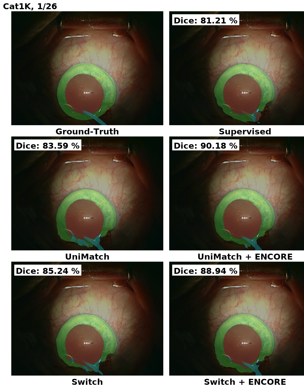
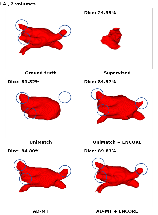
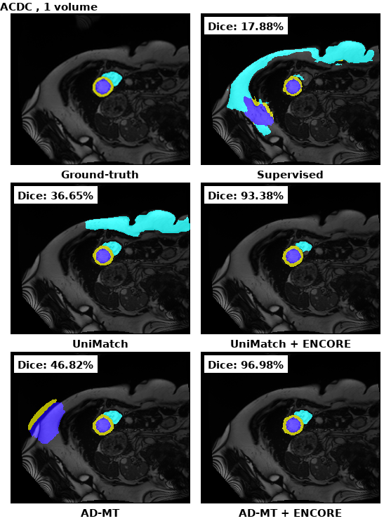
Figure 4: Qualitative comparisons of state-of-the-art methods with and without ENCORE on the Cataract-1K, LA, and ACDC datasets.

For multi-class segmentation in the ACDC dataset (Table 4), ENCORE further demonstrated its effectiveness in low-data settings. UniMatch + ENCORE trained with only one labeled volume outperformed supervised training with 10 labeled volumes. As expected, performance gains with ENCORE were most pronounced in extreme low-data settings (one and two labeled volumes); however, improvements remained consistently high across different semi-supervised learning frameworks.

Moreover, these gains were consistent across different network architectures: DeepLabV3+ for Tables 1, 2, and 3, UNet for Table 4, and VNet for Table 5. Overall, the combination of ENCORE with state-of-the-art methods consistently emerged as the top-performing approach across all reported datasets.

Ablation Study. Since ENCORE consists of two key components—Class-Aware Confidence Calibration (CAC) and Adaptive Confidence Thresholding (ACT)—we conducted an ablation study to assess their individual contributions to segmentation performance. Table 6 evaluates the impact of CAC and ACT on per-class segmentation performance in the Cataract-1K dataset using the Switch framework. While Switch alone improved the average Dice score over supervised learning, a per-class analysis revealed performance degradation for challenging classes, particularly Lens in 1/8 labeled data and Iris and Lens in 1/26 labeled data. In contrast, integrating either CAC or ACT independently improved segmentation performance across all classes. Moreover, combining both CAC and ACT yielded a significantly larger improvement compared to using each module in isolation. Table 7 presents the results of the ablation study on the ACDC and LA datasets, further reinforcing the contribution of our proposed modules in improving segmentation performance when integrated into the AD-MT framework.

Figure 4 presents qualitative comparisons between different baselines with and without ENCORE. Notably, for the LA dataset, integrating ENCORE into both UniMatch and AD-MT enhances the retrieval of important structural features in volumetric segmentation.

Figure 5 compares the Kernel Density Estimation (KDE) of the AD-MT method with and without ENCORE across three classes in the ACDC dataset. The figure illustrates that while AD-MT alone better aligns the data distributions of labeled and unlabeled samples compared to supervised training, the addition of ENCORE further bridges the distribution gap, leading to improved feature consistency.

For additional discussions, experiments, and visual comparisons, we refer reviewers to the supplementary material.

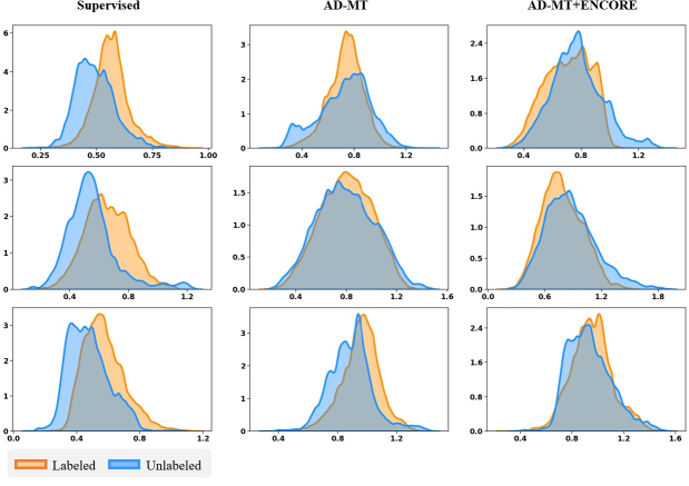
Figure 5: Kernel density estimates from various methods trained on 1 labeled ACDC dataset. From top to bottom, the plots display features corresponding to the right ventricle, myocardium, and left ventricle classes.

6 Conclusion

In this paper, we introduced Ensemble-of-Confidence Reinforcement (ENCORE), a dynamic feedback-driven pseudo-label thresholding strategy for semi-supervised semantic segmentation. Unlike conventional methods that rely on a fixed confidence threshold, ENCORE adaptively refines class-wise pseudo-label selection by leveraging a feedback mechanism. Our approach dynamically adjusts thresholds based on the student network’s performance, ensuring that informative pseudo-labels are retained while unreliable ones are filtered out. By continuously recalibrating thresholds throughout training, ENCORE mitigates overconfident noise and prevents the premature exclusion of meaningful pseudo-labels, thereby improving segmentation performance across different structures. Extensive experiments across five datasets, three network architectures, and multiple labeled data fractions, benchmarked against state-of-the-art baselines, validate the effectiveness of our method. The proposed feedback-driven pseudo-label reliability assessment method can be seamlessly integrated with pseudo-supervision frameworks, further enhancing semantic segmentation performance. In future work, we aim to extend ENCORE to broader tasks such as classification and action recognition, exploring its applicability beyond semantic segmentation.

References

- Allan et al. [2019] Max Allan, Alex Shvets, Thomas Kurmann, Zichen Zhang, Rahul Duggal, Yun-Hsuan Su, Nicola Rieke, Iro Laina, Niveditha Kalavakonda, Sebastian Bodenstedt, et al. 2017 robotic instrument segmentation challenge. arXiv preprint arXiv:1902.06426, 2019.
- Bai et al. [2023] Yunhao Bai, Duowen Chen, Qingli Li, Wei Shen, and Yan Wang. Bidirectional copy-paste for semi-supervised medical image segmentation. In Proceedings of the IEEE/CVF conference on computer vision and pattern recognition, pages 11514--11524, 2023.
- Bernard et al. [2018] Olivier Bernard, Alain Lalande, Clement Zotti, Frederick Cervenansky, Xin Yang, Pheng-Ann Heng, Irem Cetin, Karim Lekadir, Oscar Camara, Miguel Angel Gonzalez Ballester, et al. Deep learning techniques for automatic mri cardiac multi-structures segmentation and diagnosis: is the problem solved? IEEE transactions on medical imaging, 37(11):2514--2525, 2018.
- Chen et al. [2017] Liang-Chieh Chen, George Papandreou, Iasonas Kokkinos, Kevin Murphy, and Alan L Yuille. Deeplab: Semantic image segmentation with deep convolutional nets, atrous convolution, and fully connected crfs. IEEE transactions on pattern analysis and machine intelligence, 40(4):834--848, 2017.
- Chen et al. [2018] Liang-Chieh Chen, Yukun Zhu, George Papandreou, Florian Schroff, and Hartwig Adam. Encoder-decoder with atrous separable convolution for semantic image segmentation. In Proceedings of the European conference on computer vision (ECCV), pages 801--818, 2018.
- Chen et al. [2021a] Shuaijun Chen, Xu Jia, Jianzhong He, Yongjie Shi, and Jianzhuang Liu. Semi-supervised domain adaptation based on dual-level domain mixing for semantic segmentation. In Proceedings of the IEEE/CVF Conference on Computer Vision and Pattern Recognition, pages 11018--11027, 2021a.
- Chen et al. [2021b] Xiaokang Chen, Yuhui Yuan, Gang Zeng, and Jingdong Wang. Semi-supervised semantic segmentation with cross pseudo supervision. In Proceedings of the IEEE/CVF Conference on Computer Vision and Pattern Recognition, pages 2613--2622, 2021b.
- Chen et al. [2021c] Ying Chen, Xu Ouyang, Kaiyue Zhu, and Gady Agam. Mask-based data augmentation for semi-supervised semantic segmentation. arXiv preprint arXiv:2101.10156, 2021c.
- Cho et al. [2024] Hyuna Cho, Injun Choi, Suha Kwak, and Won Hwa Kim. Interactive network perturbation between teacher and students for semi-supervised semantic segmentation. In Proceedings of the IEEE/CVF Winter Conference on Applications of Computer Vision, pages 626--635, 2024.
- Deng et al. [2009] Jia Deng, Wei Dong, Richard Socher, Li-Jia Li, Kai Li, and Li Fei-Fei. Imagenet: A large-scale hierarchical image database. In 2009 IEEE conference on computer vision and pattern recognition, pages 248--255. Ieee, 2009.
- Feng et al. [2022] Zhengyang Feng, Qianyu Zhou, Qiqi Gu, Xin Tan, Guangliang Cheng, Xuequan Lu, Jianping Shi, and Lizhuang Ma. Dmt: Dynamic mutual training for semi-supervised learning. Pattern Recognition, page 108777, 2022.
- French et al. [2019] Geoff French, Samuli Laine, Timo Aila, Michal Mackiewicz, and Graham Finlayson. Semi-supervised semantic segmentation needs strong, varied perturbations. arXiv preprint arXiv:1906.01916, 2019.
- Gao et al. [2021] Li Gao, Jing Zhang, Lefei Zhang, and Dacheng Tao. Dsp: Dual soft-paste for unsupervised domain adaptive semantic segmentation. In Proceedings of the 29th ACM International Conference on Multimedia, pages 2825--2833, 2021.
- Ghamsarian et al. [2023] Negin Ghamsarian, Yosuf El-Shabrawi, Sahar Nasirihaghighi, Doris Putzgruber-Adamitsch, Martin Zinkernagel, Sebastian Wolf, Klaus Schoeffmann, and Raphael Sznitman. Cataract-1k: Cataract surgery dataset for scene segmentation, phase recognition, and irregularity detection. arXiv preprint arXiv:2312.06295, 2023.
- Ghiasi et al. [2021] Golnaz Ghiasi, Yin Cui, Aravind Srinivas, Rui Qian, Tsung-Yi Lin, Ekin D Cubuk, Quoc V Le, and Barret Zoph. Simple copy-paste is a strong data augmentation method for instance segmentation. In Proceedings of the IEEE/CVF Conference on Computer Vision and Pattern Recognition, pages 2918--2928, 2021.
- He et al. [2016] Kaiming He, Xiangyu Zhang, Shaoqing Ren, and Jian Sun. Deep residual learning for image recognition. In Proceedings of the IEEE conference on computer vision and pattern recognition, pages 770--778, 2016.
- He et al. [2017] Kaiming He, Georgia Gkioxari, Piotr Dollár, and Ross Girshick. Mask r-cnn. In Proceedings of the IEEE international conference on computer vision, pages 2961--2969, 2017.
- Hu et al. [2021] Hanzhe Hu, Fangyun Wei, Han Hu, Qiwei Ye, Jinshi Cui, and Liwei Wang. Semi-supervised semantic segmentation via adaptive equalization learning. Advances in Neural Information Processing Systems, 34:22106--22118, 2021.
- Kalluri et al. [2019] Tarun Kalluri, Girish Varma, Manmohan Chandraker, and CV Jawahar. Universal semi-supervised semantic segmentation. In Proceedings of the IEEE/CVF International Conference on Computer Vision, pages 5259--5270, 2019.
- Ke et al. [2020] Zhanghan Ke, Di Qiu, Kaican Li, Qiong Yan, and Rynson WH Lau. Guided collaborative training for pixel-wise semi-supervised learning. In European conference on computer vision, pages 429--445. Springer, 2020.
- Lai et al. [2021] Xin Lai, Zhuotao Tian, Li Jiang, Shu Liu, Hengshuang Zhao, Liwei Wang, and Jiaya Jia. Semi-supervised semantic segmentation with directional context-aware consistency. In Proceedings of the IEEE/CVF Conference on Computer Vision and Pattern Recognition, pages 1205--1214, 2021.
- Laine and Aila [2016] Samuli Laine and Timo Aila. Temporal ensembling for semi-supervised learning. CoRR, abs/1610.02242, 2016.
- Lee et al. [2013] Dong-Hyun Lee et al. Pseudo-label: The simple and efficient semi-supervised learning method for deep neural networks. In Workshop on challenges in representation learning, ICML, page 896, 2013.
- Li et al. [2021] Daiqing Li, Junlin Yang, Karsten Kreis, Antonio Torralba, and Sanja Fidler. Semantic segmentation with generative models: Semi-supervised learning and strong out-of-domain generalization. In Proceedings of the IEEE/CVF Conference on Computer Vision and Pattern Recognition, pages 8300--8311, 2021.
- Li et al. [2019] Yunsheng Li, Lu Yuan, and Nuno Vasconcelos. Bidirectional learning for domain adaptation of semantic segmentation. In 2019 IEEE/CVF Conference on Computer Vision and Pattern Recognition (CVPR), pages 6929--6938, 2019.
- Lin et al. [2014] Tsung-Yi Lin, Michael Maire, Serge Belongie, James Hays, Pietro Perona, Deva Ramanan, Piotr Dollár, and C Lawrence Zitnick. Microsoft coco: Common objects in context. In European conference on computer vision, pages 740--755. Springer, 2014.
- Liu et al. [2020] Quande Liu, Qi Dou, Lequan Yu, and Pheng Ann Heng. Ms-net: Multi-site network for improving prostate segmentation with heterogeneous mri data. IEEE Transactions on Medical Imaging, 2020.
- Liu et al. [2022] Yuyuan Liu, Yu Tian, Yuanhong Chen, Fengbei Liu, Vasileios Belagiannis, and Gustavo Carneiro. Perturbed and strict mean teachers for semi-supervised semantic segmentation. In Proceedings of the IEEE/CVF Conference on Computer Vision and Pattern Recognition, pages 4258--4267, 2022.
- Long et al. [2015] Jonathan Long, Evan Shelhamer, and Trevor Darrell. Fully convolutional networks for semantic segmentation. In Proceedings of the IEEE conference on computer vision and pattern recognition, pages 3431--3440, 2015.
- Na et al. [2024] Jaemin Na, Jung-Woo Ha, Hyung Jin Chang, Dongyoon Han, and Wonjun Hwang. Switching temporary teachers for semi-supervised semantic segmentation. Advances in Neural Information Processing Systems, 36, 2024.
- Olsson et al. [2021] Viktor Olsson, Wilhelm Tranheden, Juliano Pinto, and Lennart Svensson. Classmix: Segmentation-based data augmentation for semi-supervised learning. In Proceedings of the IEEE/CVF Winter Conference on Applications of Computer Vision (WACV), pages 1369--1378, 2021.
- Ouali et al. [2020] Yassine Ouali, Céline Hudelot, and Myriam Tami. Semi-supervised semantic segmentation with cross-consistency training. In Proceedings of the IEEE/CVF Conference on Computer Vision and Pattern Recognition, pages 12674--12684, 2020.
- Perone et al. [2019] Christian S. Perone, Pedro Ballester, Rodrigo C. Barros, and Julien Cohen-Adad. Unsupervised domain adaptation for medical imaging segmentation with self-ensembling. NeuroImage, 194:1--11, 2019.
- Sajjadi et al. [2016] Mehdi Sajjadi, Mehran Javanmardi, and Tolga Tasdizen. Regularization with stochastic transformations and perturbations for deep semi-supervised learning. Advances in neural information processing systems, 29, 2016.
- Sohn et al. [2020] Kihyuk Sohn, David Berthelot, Nicholas Carlini, Zizhao Zhang, Han Zhang, Colin A Raffel, Ekin Dogus Cubuk, Alexey Kurakin, and Chun-Liang Li. Fixmatch: Simplifying semi-supervised learning with consistency and confidence. Advances in neural information processing systems, 33:596--608, 2020.
- Sun et al. [2024] Boyuan Sun, Yuqi Yang, Le Zhang, Ming-Ming Cheng, and Qibin Hou. Corrmatch: Label propagation via correlation matching for semi-supervised semantic segmentation. In Proceedings of the IEEE/CVF Conference on Computer Vision and Pattern Recognition (CVPR), pages 3097--3107, 2024.
- Tarvainen and Valpola [2017] Antti Tarvainen and Harri Valpola. Mean teachers are better role models: Weight-averaged consistency targets improve semi-supervised deep learning results. Advances in neural information processing systems, 30, 2017.
- Tranheden et al. [2021] Wilhelm Tranheden, Viktor Olsson, Juliano Pinto, and Lennart Svensson. Dacs: Domain adaptation via cross-domain mixed sampling. In Proceedings of the IEEE/CVF Winter Conference on Applications of Computer Vision (WACV), pages 1379--1389, 2021.
- Van Gansbeke et al. [2021] Wouter Van Gansbeke, Simon Vandenhende, Stamatios Georgoulis, and Luc Van Gool. Unsupervised semantic segmentation by contrasting object mask proposals. In Proceedings of the IEEE/CVF International Conference on Computer Vision (ICCV), pages 10052--10062, 2021.
- Varsavsky et al. [2020] Thomas Varsavsky, Mauricio Orbes-Arteaga, Carole H. Sudre, Mark S. Graham, Parashkev Nachev, and M. Jorge Cardoso. Test-time unsupervised domain adaptation. In Medical Image Computing and Computer Assisted Intervention -- MICCAI 2020, pages 428--436, Cham, 2020. Springer International Publishing.
- Wang et al. [2021] Wenguan Wang, Tianfei Zhou, Fisher Yu, Jifeng Dai, Ender Konukoglu, and Luc Van Gool. Exploring cross-image pixel contrast for semantic segmentation. In Proceedings of the IEEE/CVF International Conference on Computer Vision (ICCV), pages 7303--7313, 2021.
- Wang et al. [2022] Yuchao Wang, Haochen Wang, Yujun Shen, Jingjing Fei, Wei Li, Guoqiang Jin, Liwei Wu, Rui Zhao, and Xinyi Le. Semi-supervised semantic segmentation using unreliable pseudo-labels. In Proceedings of the IEEE/CVF Conference on Computer Vision and Pattern Recognition, pages 4248--4257, 2022.
- Wang et al. [2023] Yongchao Wang, Bin Xiao, Xiuli Bi, Weisheng Li, and Xinbo Gao. Mcf: Mutual correction framework for semi-supervised medical image segmentation. In Proceedings of the IEEE/CVF conference on computer vision and pattern recognition, pages 15651--15660, 2023.
- Wei et al. [2021] Chen Wei, Kihyuk Sohn, Clayton Mellina, Alan Yuille, and Fan Yang. Crest: A class-rebalancing self-training framework for imbalanced semi-supervised learning. In Proceedings of the IEEE/CVF conference on computer vision and pattern recognition, pages 10857--10866, 2021.
- Xie et al. [2020] Qizhe Xie, Zihang Dai, Eduard Hovy, Thang Luong, and Quoc Le. Unsupervised data augmentation for consistency training. Advances in Neural Information Processing Systems, 33:6256--6268, 2020.
- Xiong et al. [2021] Zhaohan Xiong, Qing Xia, Zhiqiang Hu, Ning Huang, Cheng Bian, Yefeng Zheng, Sulaiman Vesal, Nishant Ravikumar, Andreas Maier, Xin Yang, et al. A global benchmark of algorithms for segmenting the left atrium from late gadolinium-enhanced cardiac magnetic resonance imaging. Medical image analysis, 67:101832, 2021.
- Yang et al. [2022] Lihe Yang, Wei Zhuo, Lei Qi, Yinghuan Shi, and Yang Gao. St++: Make self-training work better for semi-supervised semantic segmentation. In Proceedings of the IEEE/CVF Conference on Computer Vision and Pattern Recognition, pages 4268--4277, 2022.
- Yang et al. [2023] Lihe Yang, Lei Qi, Litong Feng, Wayne Zhang, and Yinghuan Shi. Revisiting weak-to-strong consistency in semi-supervised semantic segmentation. In Proceedings of the IEEE/CVF Conference on Computer Vision and Pattern Recognition, pages 7236--7246, 2023.
- Yun et al. [2019] Sangdoo Yun, Dongyoon Han, Seong Joon Oh, Sanghyuk Chun, Junsuk Choe, and Youngjoon Yoo. Cutmix: Regularization strategy to train strong classifiers with localizable features. In Proceedings of the IEEE/CVF international conference on computer vision, pages 6023--6032, 2019.
- Zeng et al. [2021] Xiangyun Zeng, Rian Huang, Yuming Zhong, Dong Sun, Chu Han, Di Lin, Dong Ni, and Yi Wang. Reciprocal learning for semi-supervised segmentation. In Medical Image Computing and Computer Assisted Intervention--MICCAI 2021: 24th International Conference, Strasbourg, France, September 27--October 1, 2021, Proceedings, Part II 24, pages 352--361. Springer, 2021.
- Zhao et al. [2017] Hengshuang Zhao, Jianping Shi, Xiaojuan Qi, Xiaogang Wang, and Jiaya Jia. Pyramid scene parsing network. In Proceedings of the IEEE conference on computer vision and pattern recognition, pages 2881--2890, 2017.
- Zhao et al. [2024] Zhen Zhao, Zicheng Wang, Longyue Wang, Dian Yu, Yixuan Yuan, and Luping Zhou. Alternate diverse teaching for semi-supervised medical image segmentation. In European Conference on Computer Vision, pages 227--243. Springer, 2024.
- Zhong et al. [2021] Yuanyi Zhong, Bodi Yuan, Hong Wu, Zhiqiang Yuan, Jian Peng, and Yu-Xiong Wang. Pixel contrastive-consistent semi-supervised semantic segmentation. In Proceedings of the IEEE/CVF International Conference on Computer Vision (ICCV), pages 7273--7282, 2021.
- Zhou et al. [2021] Yanning Zhou, Hang Xu, Wei Zhang, Bin Gao, and Pheng-Ann Heng. C3-semiseg: Contrastive semi-supervised segmentation via cross-set learning and dynamic class-balancing. In Proceedings of the IEEE/CVF International Conference on Computer Vision, pages 7036--7045, 2021.
- Zhou et al. [2019] Zongwei Zhou, Md Mahfuzur Rahman Siddiquee, Nima Tajbakhsh, and Jianming Liang. Unet++: Redesigning skip connections to exploit multiscale features in image segmentation. IEEE transactions on medical imaging, 39(6):1856--1867, 2019.
- Zou et al. [2018] Yang Zou, Zhiding Yu, B. V. K. Vijaya Kumar, and Jinsong Wang. Unsupervised domain adaptation for semantic segmentation via class-balanced self-training. In Computer Vision -- ECCV 2018, pages 297--313, Cham, 2018. Springer International Publishing.
- Zou et al. [2020] Yuliang Zou, Zizhao Zhang, Han Zhang, Chun-Liang Li, Xiao Bian, Jia-Bin Huang, and Tomas Pfister. Pseudoseg: Designing pseudo labels for semantic segmentation. arXiv preprint arXiv:2010.09713, 2020.