Heterogeneous Data Game: Characterizing the Model Competition Across Multiple Data Sources

Abstract

Data heterogeneity across multiple sources is common in real-world machine learning (ML) settings. Although many methods focus on enabling a single model to handle diverse data, real-world markets often comprise multiple competing ML providers. In this paper, we propose a game-theoretic framework—the Heterogeneous Data Game—to analyze how such providers compete across heterogeneous data sources. We investigate the resulting pure Nash equilibria (PNE), showing that they can be non-existent, homogeneous (all providers converge on the same model), or heterogeneous (providers specialize in distinct data sources). Our analysis spans monopolistic, duopolistic, and more general markets, illustrating how factors such as the “temperature” of data-source choice models and the dominance of certain data sources shape equilibrium outcomes. We offer theoretical insights into both homogeneous and heterogeneous PNEs, guiding regulatory policies and practical strategies for competitive ML marketplaces.

1 Introduction

Data heterogeneity is commonplace in real-world machine learning (ML) applications, where data often originate from multiple sources with distinct distributions (Li et al., 2017; Hendrycks et al., 2020; Gulrajani and Lopez-Paz, 2021; Liu et al., 2023). For example, in health care, patient data may be gathered from different hospitals, each serving varied demographics and disease prevalences. Such heterogeneous settings arise across diverse fields, including the digital economy and scientific research.

Much of the existing literature on heterogeneous data focuses on devising a single ML method that performs robustly across all data sources (Arjovsky et al., 2019; Kuang et al., 2020; Liu et al., 2021b; Duchi and Namkoong, 2021). However, real-world markets typically have multiple ML providers (Black et al., 2022; Jagadeesan et al., 2023a), each aiming to optimize its performance relative to others. For instance, competing diagnostic tool providers offer models to hospitals, which then choose a provider based on local performance criteria. This competitive interplay differs significantly from single-provider frameworks (Nisan et al., 2007) and can lead to market dynamics unaddressed by previous approaches.

Several works (Ben-Porat and Tennenholtz, 2017, 2019; Feng et al., 2022; Jagadeesan et al., 2023a; Iyer and Ke, 2024; Einav and Rosenfeld, 2025) have analyzed competition among multiple ML model providers, examining Nash equilibria, social welfare, and agents’ strategies under competition. However, these studies mainly focus on a single data distribution and do not account for heterogeneity across multiple sources.

In this paper, we develop a game-theoretic framework to study multiple providers competing over heterogeneous data sources. We then analyze the resulting pure Nash equilibria to uncover how data heterogeneity and competitive forces shape providers’ strategies.

1.1 Overview of the Heterogeneous Data Game

We introduce the Heterogeneous Data Game to model the competition among multiple ML model providers across diverse data sources. Consider $K$ distinct data sources, each associated with a weight $w_{k}$ representing its proportion, and joint distributions $P_{k}(x,y)$ over features $x$ and labels $y$. In this market, each of the $N$ ML model providers selects a model parameterized by $\hat{\theta}_{n}$. Following previous works on model and platform competition (Jagadeesan et al., 2023a; Drezner and Eiselt, 2024), the utility of each model provider is determined by its market share across the different data sources. Specifically, each data source $k$ selects an ML model based on the observed losses of available models. A provider’s utility is then the sum of $w_{k}$ from all data sources that adopt its model. Consequently, each provider strategically chooses $\hat{\theta}_{n}$ to maximize its utility.

Motivated by linear models, we represent each data source with two statistics: a ground-truth parameter $\theta_{k}$ for $P_{k}(y|x)$ and a covariance matrix $\Sigma_{k}$ for $P_{k}(x)$. From a distribution-shift perspective, variations in $\theta_{k}$ and $\Sigma_{k}$ across sources correspond to concept shift and covariate shift, respectively—two common types of distribution shifts in practice (Liu et al., 2021b). Additionally, the loss of a model $\hat{\theta}_{n}$ on data source $k$ is calculated as the squared Mahalanobis distance, $(\hat{\theta}_{n}-\theta_{k})^{\top}\Sigma_{k}(\hat{\theta}_{n}-\theta_{k})$, corresponding to the mean squared error (MSE) in linear model settings.

For data sources’ choice models, we adopt two standard frameworks (Drezner and Eiselt, 2024): the proximity choice model (Hotelling, 1929; Plastria, 2001; Ahn et al., 2004), where each data source selects the provider with the lowest loss (with ties broken uniformly), and the probability choice model (Wilson, 1975; Hodgson, 1981; Bell et al., 1998), where data sources may choose sub-optimal models based on a logit framework (Train, 2009), controlled by a temperature parameter $t$.

1.2 Overview of the Results

An overview of these results is presented in Tab. 1. We investigate the pure Nash equilibria (PNE) of the Heterogeneous Data Game and identify three patterns of PNEs across different game setups: (1) Non-existence of PNE. In this case, no PNE exists, leading to an unstable ML model market. (2) Homogeneous PNE. Here, all model providers independently train their ML models to minimize the $w_{k}$-weighted loss across all data sources. As a result, this type of PNE leads to the homogeneity of models available in the market. (3) Heterogeneous PNE. In this scenario, model providers offer different ML models. Most specialize in a single data source, typically adopting the ground-truth parameter $\theta_{k}$ of a specific data source $k$.

Monopoly ($N=1$).

In this setting, a single provider can achieve the same utility with any ML model parameter. However, it typically chooses the parameter that minimizes the weighted loss across all data sources, denoted by $\hat{\theta}^{\text{M}}$.

Duopoly ($N=2$).

Under the proximity choice model, we specify conditions for the existence of a PNE and show that, if a PNE exists, both providers choose the ground-truth parameter of the data source with the maximal weight. In contrast, under the probability choice model, any PNE must be homogeneous, with both providers choosing $\hat{\theta}^{\text{M}}$, the parameter that minimizes the weighted loss across sources.

	Heterogeneous Data Game under the Proximity Choice Model	Heterogeneous Data Game under the Probability Choice Model
Monopoly ($N=1$)	The single model chooses the parameter given by Eq. 9.
Duopoly ($N=2$)	Equivalent condition for PNE existence (Thm. 5.1) PNE must be heterogeneous, if it exists (Thm. 5.1)	Equivalent condition for PNE existence (Thm. 5.2) PNE must be homogeneous, if it exists (Thm. 5.2)
$N>2$	Sufficient condition for PNE existence (Thms. 5.4 and 5.5) PNE must be heterogeneous, if it exists (Prop. 5.3)	Equivalent condition for homogeneous PNE existence (Thm. 5.6) Sufficient condition for heterogeneous PNE existence (Thm. 5.7) Example when both types of PNE exist simultaneously (Ex. 5.2)

Table 1: Overview of the results.

More than two providers ($N>2$).

Under the proximity choice model, if a PNE exists, providers tend to pick different models, leading to a heterogeneous PNE. Moreover, when a few data sources have significantly larger weights (Kairouz et al., 2021; Li et al., 2020), a PNE exists if $N$ lies within a certain range, and providers fully specialize in those dominant sources. In contrast, under the probability choice model, both homogeneous and heterogeneous PNE may arise, depending on the temperature $t$. Specifically, when $t$ is small, indicating that data sources are highly unlikely to choose sub-optimal models, only a heterogeneous PNE may exist. Conversely, when $t$ is large, meaning data sources are more likely to uniformly choose among all available models, only a homogeneous PNE may exist. We also present an example where both types of PNE exist simultaneously.

Our theoretical findings yield several insights for multi-provider ML markets. First, they illuminate how the interplay of data heterogeneity, choice models, and competition can produce either homogeneous or heterogeneous equilibria, thereby influencing the variety of models offered. Second, they indicate that when a few data sources dominate, providers tend to specialize in those sources, potentially overlooking smaller ones; this outcome calls for appropriate incentive mechanisms. Finally, market parameters—such as the temperature in the probability choice model—can be adjusted by market regulators to foster either heterogeneous model offerings or convergence toward homogeneous solutions. Taken together, these insights can inform both regulatory policy and practical strategies for building competitive ML marketplaces.

2 Related Works

Data heterogeneity.

In real-world scenarios, data often exhibit significant heterogeneity due to variations in time, space, and population during the data collection process (Liu et al., 2023). The concept of data heterogeneity has been extensively studied across multiple disciplines, including ecology (Li and Reynolds, 1995), economics (Rosenbaum, 2005), and computer science (Wang et al., 2019). This work focuses on the implications of data heterogeneity in machine learning settings. In this context, considerable research has aimed to ensure that a single model performs robustly across diverse test environments (Liu et al., 2021b), leading to a range of effective methodological frameworks, including causal learning (Bühlmann, 2020; Peters et al., 2016), invariant learning (Arjovsky et al., 2019; Liu et al., 2021a; Koyama and Yamaguchi, 2020), stable learning (Xu et al., 2022; Kuang et al., 2020; Yu et al., 2023), and distributionally robust optimization (Sinha et al., 2018; Duchi and Namkoong, 2021; Liu et al., 2022). However, these existing approaches largely overlook the presence of multiple competing model providers and the strategic interactions that arise in such settings.

Competition in machine learning.

Our work extends prior research on competition among machine learning model providers under homogeneous data settings (Ben-Porat and Tennenholtz, 2017, 2019; Feng et al., 2022; Jagadeesan et al., 2023a; Einav and Rosenfeld, 2025). Specifically, Ben-Porat and Tennenholtz (2017, 2019) studied best-response dynamics and algorithmic methods for finding pure Nash equilibria (PNE) in regression tasks, while Einav and Rosenfeld (2025) extended these insights to classification. Feng et al. (2022) explored the bias–variance trade-off in competitive environments, showing that competing agents tend to favor variance-induced error over bias. Jagadeesan et al. (2023a) demonstrated that increasing model size does not necessarily improve social welfare. In contrast to these studies, we consider heterogeneous data sources with distinct distributions, uncovering novel equilibrium structures and establishing new conditions for their existence.

Competitive location models.

Our framework is technically related to competitive location models (Hotelling, 1929; Shaked, 1975; d’Aspremont et al., 1979; Eiselt et al., 1993; Plastria, 2001; Ahn et al., 2004), as comprehensively surveyed by Drezner and Eiselt (2024). However, most existing models focus on low-dimensional spaces or networks with uniform distance metrics, largely due to two factors: (1) applications in urban planning naturally align with one-dimensional (Hotelling, 1929; d’Aspremont et al., 1979), two-dimensional (Tsai and Lai, 2005; Shaked, 1975; Lederer and Hurter Jr, 1986), or network-based (Eiselt and Laporte, 1991, 1993; Dorta-González et al., 2005) formulations; and (2) many models incorporate additional variables such as price or quantity, which reduce tractability and restrict attention to small-scale settings. While a few studies investigate high-dimensional competition, they primarily address quantity competition (Anderson and Neven, 1990) or pricing (Bester, 1989), rather than spatial or parameter-based competition. By contrast, our setting considers source-specific distance metrics arising from distributional shifts, along with high-dimensional strategy spaces driven by a large number of data sources and model parameters. These distinctions introduce substantial challenges for theoretical analysis.

Other competitive frameworks.

Finally, our work connects to competition scenarios in targeted advertising (Iyer and Ke, 2024; Iyer et al., 2024), online marketplaces (Liu et al., 2020; Hron et al., 2023; Jagadeesan et al., 2023b; Yao et al., 2024a, b), platform competition (Jullien and Sand-Zantman, 2021; Calvano and Polo, 2021), and broader game-theoretic analyses (Immorlica et al., 2011). Unlike these studies, we highlight how heterogeneous data distributions shape market equilibria among multiple ML model providers.

3 Heterogeneous Data Game (HD-Game)

3.1 Notations

We begin by introducing several essential notations. For a positive integer $N$, let $[N]$ denote the set $\{1,2,\dots,N\}$. The $N$-dimensional simplex, denoted by $\Delta_{N}$, is defined as $\Delta_{N}=\{(x_{1},x_{2},\dots,x_{N}):\sum_{i=1}^{N}x_{i}=1\text{ and }x_{i}\geq 0,\forall i\in[N]\}$. For any square matrix $A$, we use $A\succ 0$ to indicate that $A$ is positive definite, and $A\succeq 0$ to indicate that $A$ is positive semi-definite. Furthermore, given a positive definite square matrix $\Sigma\succ 0$, the Mahalanobis distance between two vectors $x$ and $y$ is defined as $d_{M}(x,y;\Sigma)=\sqrt{(x-y)^{\top}\Sigma^{-1}(x-y)}$.

3.2 Game Setup

Heterogeneous data.

Consider a setting with $K\geq 2$ data sources. Each source $k$ has a true model parameter $\theta_{k}\in\mathbb{R}^{D}$ and a covariance matrix $\Sigma_{k}$. These two terms capture concept shift (via $\theta_{k}$) and covariate shift (via $\Sigma_{k}$), respectively (Liu et al., 2021b), as detailed in Sec. 3.3. We further assume $\theta_{k}\neq\theta_{k^{\prime}}$ for all $k\neq k^{\prime}$, since any two sources with identical parameters can be merged into one.

For a model parameterized by $\theta\in\mathbb{R}^{D}$, the loss associated with data source $k$ is defined as the squared Mahalanobis distance between $\theta$ and $\theta_{k}$ with $\Sigma_{k}^{-1}$, i.e., $d_{M}^{2}(\theta,\theta_{k};\Sigma_{k}^{-1})$. As shown in Sec. 3.3, the Mahalanobis distance could correspond to the mean square error (MSE) of $\theta$ on data source $k$ in linear model settings, and it can measure the error caused by both concept shift and covariate shift.

Additionally, each data source $k$ is assigned a weight $w_{k}$, representing its proportion within the total data. Without loss of generality, we assume the weights are ordered and $w_{1}>w_{2}>\dots>w_{K}>0$, with $\sum_{k=1}^{K}w_{k}=1$. Let $\boldsymbol{w}=(w_{1},w_{2},\dots,w_{K})$ denote the vector of weights.

Model providers.

There are $N$ model providers (players) that need to compete the models in these $K$ data sources. Each player $n\in[N]$ needs to choose one model $\hat{\theta}_{n}\in\mathbb{R}^{D}$, and the loss of player $n$ for data source $k$, denoted as $\ell_{n,k}$, is

$$\ell_{n,k}=d_{M}^{2}(\hat{\theta}_{n},\theta_{k};\Sigma_{k}^{-1})=(\hat{\theta}_{n}-\theta_{k})^{\top}\Sigma_{k}(\hat{\theta}_{n}-\theta_{k}).$$ (1)

Data sources’ choice model.

The data sources will choose which model to deploy based on the losses $\ell_{n,k}$. Formally, let $g:\mathbb{R}^{N}\rightarrow\Delta_{N}$ be the choice model. For a data source $k$, given $N$ losses $\ell_{1,k},\ell_{2,k},\dots,\ell_{N,k}$, the function $g(\ell_{1,k},\dots,\ell_{N,k})$ will output an $N$-dimensional vector, and its $n$-th element, denoted as $g_{n}(\ell_{1,k},\dots,\ell_{N,k})$, is the probability of choosing the $n$-th model. Following previous works (Jagadeesan et al., 2023a; Drezner and Eiselt, 2024), we consider two types of choice models for estimating the market share of different participants:

• Proximity choice model. Here, each data source chooses the model with the least loss. When several models exhibit the same loss, the data source will randomly choose one model with equal probabilities. Formally,

  $$g_{n}^{\text{PROX}}(\ell_{1,k},\dots,\ell_{N,k})=\begin{cases}0,&\text{if }\exists j\in[N],\ell_{j,k}<\ell_{n,k}\\ \frac{1}{\left|\left\{j\in[N]:\ell_{j,k}=\ell_{n,k}\right\}\right|},&\text{otherwise}.\end{cases}$$ (2)

• Probability choice model. Following (Jagadeesan et al., 2023a), we assume that data sources may noisily choose the models based on the following logit model (Train, 2009),

  $$g_{n}^{\text{PROP}}(\ell_{1,k},\dots,\ell_{N,k})=\frac{\exp(-\ell_{n,k}/t)}{\sum_{j=1}^{N}\exp(-\ell_{j,k}/t)}.$$ (3)

  with a temperature parameter $t>0$. Intuitively, the parameter $t$ controls the willingness for each data source to choose sub-optimal models. When $t\rightarrow 0$, this model will become the proximity model as shown in Eq. 2. By contrast, when $t\rightarrow\infty$, all models become indifferent and the data source tends to choose models randomly.

The Heterogeneous Data Game.

Given a strategy profile $\hat{\boldsymbol{\theta}}=(\hat{\theta}_{1},\hat{\theta}_{2},\dots,\hat{\theta}_{N})$, the utility of player $n$ is

$$u_{n}(\hat{\boldsymbol{\theta}})=\sum_{k=1}^{K}w_{k}g_{n}(\ell_{1,k},\dots,\ell_{N,k}).$$ (4)

We note that for each $n\in[N]$, the term $\ell_{n,k}$ is implicitly a function of $\hat{\theta}_{n}$, as defined in Eq. 1. For any $\theta\in\mathbb{R}^{D}$, we use $(\theta,\hat{\boldsymbol{\theta}}_{-n})$ to denote the strategy profile in which player $n$ deviates from their original strategy $\hat{\theta}_{n}$ to a new strategy $\theta\in\mathbb{R}^{D}$. We focus on the properties of the Pure Nash Equilibrium (PNE), formally defined as follows.

Definition 3.1 (Pure Nash Equilibrium (PNE)).

A strategy profile $\hat{\boldsymbol{\theta}}=(\hat{\theta}_{1},\dots,\hat{\theta}_{N})$ is a pure Nash equilibrium if, for all $n\in[N]$ and $\theta\in\mathbb{R}^{D}$, $u_{n}(\theta,\hat{\boldsymbol{\theta}}_{-n})\leq u_{n}(\hat{\boldsymbol{\theta}})$.

In practice, model providers incur significant costs when retraining multiple models and typically deploy a single model rather than adopting a mixed strategy. Consequently, it is more realistic to analyze the pure Nash equilibrium (PNE), where each provider commits to a specific model, rather than the mixed Nash equilibrium (MNE), which assumes randomized selection among multiple models.

Note that the utility function depends on whether the choice model $g_{n}(\cdot)$ in Eq. 4 is set as $g_{n}^{\text{PROX}}$ or $g_{n}^{\text{PROP}}$, as defined in Eqs. 2 and 3. Consequently, different choice models yield different games and, therefore, different PNEs. For clarity, we refer to the heterogeneous data game under the proximity choice model as HD-Game-Proximity and under the probability choice model as HD-Game-Probability in the remainder of this paper.

3.3 Motivating Example — Linear Model

Consider a linear model setting with $K$ data sources, each associated with a distribution $P_{k}(x,y)$ for $k\in[K]$, where $x\in\mathbb{R}^{D}$ denotes the feature vector and $y\in\mathbb{R}$ is the corresponding label. Assume that $x$ is normalized such that $\mathbb{E}_{P_{k}}[x]=0$. The covariance matrix under $P_{k}$ is then given by $\Sigma_{k}=\mathbb{E}_{P_{k}}[xx^{\top}]\succ 0$. Furthermore, assume that the conditional distribution $P_{k}(y\mid x)$ follows a linear model with parameter $\beta_{k}$, perturbed by Gaussian noise $\varepsilon\sim\mathcal{N}(0,\sigma_{k}^{2})$; that is, $y\mid x\sim\mathcal{N}(\beta_{k}^{\top}x,\sigma_{k}^{2})$.

Consider $N$ players, each selecting a parameter $\hat{\beta}_{n}$. The MSE of player $n$ on data source $k$ is given by

$$\mathbb{E}_{P_{k}}\left[\left(\hat{\beta}_{n}^{\top}x-y\right)^{2}\right]=\left(\hat{\beta}_{n}-\beta_{k}\right)^{\top}\Sigma_{k}\left(\hat{\beta}_{n}-\beta_{k}\right)+\sigma_{k}^{2}=d_{M}^{2}\left(\hat{\beta}_{n},\beta_{k};\Sigma_{k}^{-1}\right)+\sigma_{k}^{2}.$$ (5)

It is easy to verify that the noise term in Eq. 5 does not affect the choice models in Eqs. 2 and 3. Consequently, we confirm that using the squared Mahalanobis distance as a loss function aligns with the mean squared error (MSE), validating that the game effectively characterizes model provider competition in linear settings.

Moreover, linear probing—where only the final linear layer is updated—is a widely used technique for adapting pretrained models to downstream tasks, particularly when fine-tuning the full model is computationally expensive or prone to overfitting (Kumar et al., 2022). Since features $x$ can represent either raw inputs or embeddings from pretrained models, our framework also extends to scenarios where model providers employ the linear probing technique.

4 Basic Properties and Assumptions

4.1 Basic Properties of HD-Game

We first characterize the possible strategy set in equilibria for each player.

Proposition 4.1.

Denote the set $\vartheta$ as follows:

$$\vartheta\triangleq\left\{\bar{\theta}(\boldsymbol{q}):\boldsymbol{q}=(q_{1},q_{2},\dots,q_{K})\in\Delta_{K}\right\},$$ (6)

where

$$\bar{\theta}(\boldsymbol{q})\triangleq\operatorname*{arg\,min}_{\theta}\sum_{k=1}^{K}q_{k}d_{M}^{2}\left(\theta,\theta_{k};\Sigma_{k}^{-1}\right)=\left(\sum_{k=1}^{K}q_{k}\Sigma_{k}\right)^{-1}\left(\sum_{k=1}^{K}q_{k}\Sigma_{k}\theta_{k}\right).$$ (7)

Then, the following holds:

• In HD-Game-Proximity, if a PNE exists, there must be one where every player’s strategy belongs to $\vartheta$.

• In HD-Game-Probability, any PNE necessarily requires all players’ strategies to lie within $\vartheta$.

Remark 4.1.

Prop. 4.1 suggests that players will generally choose strategies from the set $\vartheta$, which corresponds to minimizing a weighted loss over data sources, with each player determining their respective weights.

4.2 Assumptions

We introduce the following regularity assumption.

Assumption 4.1.

For any $\theta\in\mathbb{R}^{D}$, there is at most one $\boldsymbol{q}\in\Delta_{K}$ such that $\bar{\theta}(\boldsymbol{q})=\theta$.

Remark 4.2.

When $\Sigma_{1}=\Sigma_{2}=\cdots=\Sigma_{K}$, this assumption reduces to requiring that $\theta_{1},\theta_{2},\dots,\theta_{K}$ be affinely independent. For general settings, the number of parameters $D$ is typically large, whereas the number of data sources $K$ is relatively small, often satisfying $K\leq D$. Consequently, this assumption is generally reasonable in real-world settings.

Assumption 4.2.

For all $i,j,k\in[K]$ with $i\neq j$, $d_{M}(\theta_{i},\theta_{k};\Sigma_{k}^{-1})\neq d_{M}(\theta_{j},\theta_{k};\Sigma_{k}^{-1})$.

Remark 4.3.

This assumption ensures that no two ground-truth models $\theta_{i}$ and $\theta_{j}$ from distinct data sources have identical losses on a given data source $k$. Since different data sources typically have distinct ground-truth models, this condition is generally satisfied in practice.

Problem-dependent constants.

We introduce the following constant based on the game’s parameters:

$$\ell_{\max}\triangleq\max_{\theta\in\vartheta,k\in[K]}d_{M}^{2}(\theta,\theta_{k};\Sigma_{k}^{-1}),$$ (8)

which represents the maximum possible loss for any strategy in $\vartheta$. Intuitively, $\ell_{\max}$ quantifies the degree of heterogeneity among data sources. A small $\ell_{\max}$ indicates that any model $\theta\in\vartheta$ incurs relatively low loss across all data sources, suggesting minimal variation among them. Conversely, a large $\ell_{\max}$ implies greater difficulty in finding a single model that performs well across all sources, representing higher data heterogeneity.

5 Pure Nash Equilibria Analysis

In this section, we formally characterize the pure Nash equilibria (PNE) of our Heterogeneous Data Game under the different data-source choice models introduced earlier. As previewed in the introduction, we establish three possible outcomes, each governed by distinct sufficient conditions:

1. Non-existence of PNE. In certain settings, no PNE arises, indicating that the model market remains fundamentally unstable. In other words, providers continually adjust their strategies in response to each other, preventing any long-term equilibrium.

2. Homogeneous PNE. Here, a stable equilibrium exists in which all model providers converge on the same parameter (e.g., the one minimizing the $w_{k}$-weighted loss across sources). This outcome yields a market dominated by essentially one “universal” model.

3. Heterogeneous PNE. Here, model providers differentiate themselves by specializing in distinct data sources. Typically, each provider adopts the ground-truth parameter $\theta_{k}$ of one source, resulting in a diverse array of models.

We observe that the concepts of “homogeneous PNE” and “heterogeneous PNE” are analogous to the ideas of “minimal” and “maximal” differentiation in location theory (Drezner and Eiselt, 2024). However, we maintain the terms “homogeneous” and “heterogeneous” because our distance metric differs across data sources.

Below, we present the theoretical results for each outcome in the contexts of monopoly (Sec. 5.1), duopoly (Sec. 5.2), and general multi-provider markets (Sec. 5.3).

5.1 Monopoly Setting

When $N=1$, the model choice is arbitrary, as there is no competition. However, the model provider typically selects a strategy that minimizes the overall loss across all data sources. Consequently, the chosen strategy, denoted as $\hat{\theta}^{\text{M}}$, is given by:

$$\hat{\theta}^{\text{M}}\triangleq\bar{\theta}(\boldsymbol{w})=\operatorname*{arg\,min}_{\theta}\sum_{k=1}^{K}w_{k}d_{M}^{2}\left(\theta,\theta_{k};\Sigma_{k}^{-1}\right).$$ (9)

5.2 Duopoly Setting

In this subsection, we consider the duopoly setting where there are only $2$ model providers in the market.

5.2.1 HD-Game-Proximity

Theorem 5.1.

Consider HD-Game-Proximity with $N=2$, and suppose Assump. 4.1 holds. Then:

1. If $w_{1}<0.5$, a PNE does not exist.

2. If $w_{1}\geq 0.5$, a PNE exists, and $\hat{\boldsymbol{\theta}}=(\theta_{1},\theta_{1})$ is a PNE. Moreover, if $w_{1}>0.5$, $(\theta_{1},\theta_{1})$ is the unique PNE.

Remark 5.1.

Thm. 5.1 shows that in HD-Game-Proximity with $N=2$, a PNE exists if and only if $w_{1}\geq 0.5$, indicating the presence of a dominant data source. Moreover, when $w_{1}>0.5$, both model providers specialize in the dominant data source by selecting $\theta_{1}$.

Although both providers adopt the same strategy, this PNE is still classified as heterogeneous, consistent with the general HD-Game-Proximity results in Sec. 5.3. Notably, unlike the homogeneous PNE in HD-Game-Probability, players in this PNE specialize in a single dominant data source rather than optimizing across all sources.

5.2.2 HD-Game-Probability

Theorem 5.2.

Consider HD-Game-Probability with $N=2$, and suppose Assump. 4.1 holds. If a PNE exists, then the only possible PNE is that both players choose $\hat{\theta}^{\text{M}}$ (defined in Eq. 9).

Furthermore, there exists a constant $\underline{t}\leq 2\ell_{\max}$, depending on all game parameters, such that $\hat{\theta}^{\text{M}}$ is a PNE if and only if $t\geq\underline{t}$.

Remark 5.2.

Compared to Thm. 5.1, in HD-Game-Probability, a PNE may fail to exist even if $w_{1}\geq 0.5$ when $t$ is smaller than the threshold $\underline{t}$. This may seem counterintuitive, as one might expect the probability choice model to converge to the proximity choice model as $t\to 0$. However, the properties of PNEs are not consistent in this limit. This inconsistency arises because, for $N=2$, the only possible PNE requires both players to choose $\hat{\theta}^{\text{M}}$, as established in the first part of this theorem. Notably, this inconsistency may not hold for $N>2$, which we demonstrate in Thm. 5.7.

Deriving a closed-form expression for the threshold $\underline{t}$ is generally intractable. Empirically, we observe that $\underline{t}\approx C_{0}\cdot(2\ell_{\max})$ with $0<C_{0}<1$, where $C_{0}$ depends on the game’s parameters. Experiments (see Sec. 6) consistently show that greater data-source heterogeneity—measured by $\ell_{\max}$ in Eq. 8—pushes the threshold $\underline{t}$ upward. Hence, as heterogeneity grows, a homogeneous PNE can arise only when data sources exhibit an even stronger tendency to select sub-optimal models.

5.3 General Cases with More than Two Model Providers

In this subsection, we analyze ML model markets with more than two model providers.

5.3.1 HD-Game-Proximity

Heterogeneity in PNE.

We first show that in HD-Game-Proximity, any existing PNE tends to be heterogeneous.

Proposition 5.3.

Consider HD-Game-Proximity, and suppose Assump. 4.1 holds. Let $\hat{\boldsymbol{\theta}}=\{\hat{\theta}_{1},\dots,\hat{\theta}_{N}\}$ be a PNE. For any $\theta\in\mathbb{R}^{D}$ such that $\theta\not\in\{\theta_{1},\dots,\theta_{K}\}$, let $m=|\{j:\hat{\theta}_{j}=\theta\}|$. Then, $m\leq 1$.

Remark 5.3.

Prop. 5.3 shows that in HD-Game-Proximity, if a PNE exists, no two players will adopt the same model unless it corresponds to a ground-truth model of a data source. This suggests that model providers tend to offer distinct models, leading to a heterogeneous PNE.

Moreover, in some cases, achieving a PNE requires certain players to select strategies outside the set $\{\theta_{1},\theta_{2},\dots,\theta_{K}\}$. A detailed example is provided in App. A.

Sufficient conditions for the existence of heterogeneous PNE.

We derive sufficient conditions under which a heterogeneous PNE exists and can be explicitly characterized.

Theorem 5.4.

Consider HD-Game-Proximity and suppose that Assumps. 4.1 and 4.2 hold. Assume there exists a constant $k_{0}\in[K]$ such that $w_{k_{0}}>3\sum_{j=k_{0}+1}^{K}w_{j}$. Then PNE exists if $N$ satisfies

$$\sum_{k=1}^{k_{0}}\left\lfloor\frac{3w^{\prime}_{k}}{w^{\prime}_{k_{0}}}\right\rfloor\leq N\leq\sum_{k=1}^{k_{0}}\left(\left\lceil\frac{w^{\prime}_{k}}{\sum_{j=k_{0}+1}^{K}w_{j}}\right\rceil-1\right)$$ (10)

where for any $k$ such that $1\leq k\leq k_{0}$,

$$w^{\prime}_{k}=w_{k}+\sum_{j=k_{0}+1}^{K}w_{j}\mathbbm{1}\left[k=\operatorname*{arg\,min}_{1\leq j^{\prime}\leq k_{0}}d_{M}\left(\theta_{j^{\prime}},\theta_{k};\Sigma_{j}^{-1}\right)\right].$$ (11)

Moreover, for any PNE $\hat{\boldsymbol{\theta}}=(\hat{\theta}_{1},\dots,\hat{\theta}_{N})$, it must hold that $\forall n\in[N],\hat{\theta}_{n}\in\{\theta_{1},\theta_{2},\dots,\theta_{k_{0}}\}$. In addition, let $m_{k}=|\{j\in[N]:\hat{\theta}_{j}=\theta_{k}\}|$ be the number of players choosing strategy $\theta_{k}$ in the PNE. Then,

$$\forall k\in[k_{0}],\left|m_{k}-\left\lfloor\frac{w^{\prime}_{k}}{z^{*}}\right\rfloor\right|\leq 1$$ (12)

where $z^{*}=\sup\left\{z>0:h(z)\triangleq\sum_{k=1}^{k_{0}}\left\lfloor w^{\prime}_{k}/z\right\rfloor\geq N\right\}$.

Remark 5.4.

Thm. 5.4 suggests that when a few data sources carry dominant weights—a phenomenon commonly observed in practice (Kairouz et al., 2021; Li et al., 2020)—and the number of model providers $N$ lies within a certain range, a PNE exists in which all providers specialize in serving a single data source. Moreover, in such equilibria, the number of providers allocated to each source is approximately proportional to its weight.

Concretely, the choice of $k_{0}$ indicates that the top-$k_{0}$ data sources hold significantly higher weights, each at least three times the total weight of the remaining data sources. The constraints on $N$ in Eq. 10 ensure that (1) providers consider the $k_{0}$-th data source and (2) data sources with small weights are overlooked. Under these conditions, the exact form of the PNE can be derived. In a PNE, all model providers select a ground-truth model from the top-$k_{0}$ data sources. Consequently, the utility of non-dominant data sources is assigned to the nearest dominant data source, as characterized by Eq. 11. Furthermore, since $z^{*}$ is fixed in Eq. 12, $m_{k}$ is proportional to $w^{\prime}_{k}$. This aligns with intuition, as data sources with higher weights typically attract more model providers optimizing for them.

This insight implies that policymakers can mitigate imbalanced attention among different data sources by either introducing more providers or incentivizing focus on underrepresented sources. Thm. 5.4 provides a quantitative foundation for both interventions.

We further provide an example to explain Thm. 5.4.

Example 5.1.

Consider a setting with $K=4$ data sources and weights $\boldsymbol{w}=(0.6,0.35,0.03,0.02)$. The ground-truth models are given by $\theta_{1}=(1,0,0)$, $\theta_{2}=(-1,0,0)$, $\theta_{3}=(1,0.1,0)$, and $\theta_{4}=(-1,0,0.1)$, with covariance matrices $\Sigma_{1}=\Sigma_{2}=\Sigma_{3}=\Sigma_{4}=I$. In this case, the first two data sources have dominant weights.

Setting $k_{0}=2$, a heterogeneous PNE is guaranteed to exist when $N$ lies within a specific range ($[8,19]$ in this case). In this PNE, model providers will only select strategies from $\{\theta_{1},\theta_{2}\}$. Since data source $3$ has a similar ground-truth model to data source $1$, and data source $4$ to data source $2$, providers selecting $\theta_{1}$ benefit from data source $3$, while those selecting $\theta_{2}$ benefit from data source $4$.

For instance, when $N=10$, the PNE consists of six players choosing $\theta_{1}$ and four choosing $\theta_{2}$, approximately proportional to $(w^{\prime}_{1},w^{\prime}_{2})$, where $w^{\prime}_{1}=w_{1}+w_{3}=0.63$ and $w^{\prime}_{2}=w_{2}+w_{4}=0.37$.

In addition, Thm. 5.4 implies the following corollary.

Corollary 5.5.

Consider HD-Game-Proximity and suppose that Assumps. 4.1 and 4.2 hold. When $N\geq\sum_{k=1}^{K}\left\lfloor 3w_{k}/w_{K}\right\rfloor$, a PNE exists. Moreover, for any PNE $\hat{\boldsymbol{\theta}}=(\hat{\theta}_{1},\dots,\hat{\theta}_{N})$, it holds that $\forall n\in[N],\hat{\theta}_{n}\in\{\theta_{1},\theta_{2},\dots,\theta_{K}\}$. In addition, let $m_{k}=|\{j\in[N]:\hat{\theta}_{j}=\theta_{k}\}|$ be the number of players that choose strategy $\theta_{k}$ in the PNE. We have $\forall k\in[K]$, $\left|m_{k}-\left\lfloor w_{k}/z^{*}\right\rfloor\right|\leq 1$ where $z^{*}=\sup\left\{z>0:\sum_{k=1}^{K}\left\lfloor w_{k}/z\right\rfloor\geq N\right\}$.

Remark 5.5.

This result follows directly from Thm. 5.4 with $k_{0}$ set to $K$. It implies that a PNE always exists when $N$ is sufficiently large.

5.3.2 HD-Game-Probability

Unlike HD-Game-Proximity, we show that both homogeneous and heterogeneous PNEs can exist in HD-Game-Probability.

Homogeneous PNE.

We first derive equivalent conditions for the existence of a homogeneous PNE, as well as a sufficient condition for its uniqueness.

Theorem 5.6.

Consider HD-Game-Probability and suppose that Assump. 4.1 holds. Let $\hat{\boldsymbol{\theta}}^{\text{Homo}}=(\hat{\theta}^{\text{M}},\hat{\theta}^{\text{M}},\dots,\hat{\theta}^{\text{M}})$, where $\hat{\theta}^{\text{M}}$ is defined in Eq. 9. Then there exist two constants: $0<\underline{t}\leq 2\ell_{\max}$, depending on all game parameters, and $C>0$, depending only on $\{\Sigma_{k},\theta_{k},w_{k}\}_{k=1}^{K}$, such that the following results hold:

1. $\hat{\boldsymbol{\theta}}^{\text{Homo}}$ is a PNE if and only if $t\geq\underline{t}$.

2. If $t\geq\max\{6C/N,2\ell_{\max}\}$, then $\hat{\boldsymbol{\theta}}^{\text{Homo}}$ is the unique PNE.

Remark 5.6.

Thm. 5.6 implies that a homogeneous PNE does not exist when $t$ is small. As $t$ increases, a homogeneous PNE may emerge, and for sufficiently large $t$, it becomes the unique PNE. The closed-form expressions of $\underline{t}$ and $C$ are difficult to derive. However, similar to Thm. 5.2, synthetic experiments in Sec. 6 suggest that the threshold $\underline{t}$ required for PNE existence is approximately $C_{0}\times(2\ell_{\max})$, where $0<C_{0}<1$ is a game-specific constant. Moreover, as $N$ increases, a homogeneous PNE is more likely to be unique, as indicated by the second part of Thm. 5.6. This trend is further verified by our synthetic experiments in Sec. 6.

Heterogeneous PNE.

We next demonstrate that for sufficiently small $t$, a heterogeneous PNE can exist.

Theorem 5.7.

Consider HD-Game-Probability, and suppose that Assumps. 4.1 and 4.2 hold, with $N\geq\sum_{k=1}^{K}\left\lfloor 3w_{k}/w_{K}\right\rfloor$. Additionally, assume that for all $n,n^{\prime}\in[N]$ and distinct $k,k^{\prime}\in[K]$, it holds that $w_{k}/n\neq w_{k^{\prime}}/n^{\prime}.$ Let $\hat{\boldsymbol{\theta}}^{\text{Prox}}=(\hat{\theta}^{\text{Prox}}_{1},\dots,\hat{\theta}^{\text{Prox}}_{N})$ be a PNE in the corresponding HD-Game-Proximity. Then, there exists a constant $t^{\prime}>0$ such that for any $t\leq t^{\prime}$, a PNE $\hat{\boldsymbol{\theta}}^{\text{Hete}}=(\hat{\theta}^{\text{Hete}}_{1},\dots,\hat{\theta}^{\text{Hete}}_{N})$ exists in HD-Game-Probability and satisfies

$$\forall n\in[N],\quad\left\|\hat{\theta}^{\text{Hete}}_{n}-\hat{\theta}^{\text{Prox}}_{n}\right\|_{2}\leq t^{2}.$$

Remark 5.7.

For simplicity, we build on the conditions of Cor. 5.5. Thm. 5.7 establishes that when $t$ is sufficiently small, a heterogeneous PNE exists and closely approximates the PNE in the corresponding HD-Game-Proximity. This is expected, as HD-Game-Probability approaches HD-Game-Proximity for large $N$ as $t\to 0$. However, proving this result is significantly more challenging due to the continuous nature of the potential strategy set for each model provider.

Additionally, while the specified range for $N$ is sufficient, it is not necessary. Our experiments in Sec. 6 suggest that a heterogeneous PNE may also exist for smaller values of $N$.

Thms. 5.6 and 5.7 show that, to promote model diversity (i.e., the emergence of heterogeneous PNE) and prevent convergence to a single dominant model (i.e., homogeneous PNE), policymakers can increase the rationality of data sources—that is, enhance their ability to select higher-performing models—which, in turn, encourages the formation of heterogeneous PNE.

Existence of both PNE at the same time.

We now present an example to illustrate that both types of PNE can coexist in a single game.

Example 5.2.

Let $N=8$ and $K=2$ with $\theta_{1}=(1,1)$ and $\theta_{2}=(0,1)$. The covariance matrices are $\Sigma_{1}=\Sigma_{2}=I$, and the weights are $\boldsymbol{w}=(0.53,0.47)$. The temperature parameter is set to $t=0.4$. Since $K=2$, Prop. 4.1 implies that each model provider selects a weight $\alpha_{n}\in[0,1]$, yielding the final model $\hat{\theta}_{n}=\alpha_{n}\theta_{1}+(1-\alpha_{n})\theta_{2}=(\alpha_{n},1)$.

In this setting, we identify two types of PNE: (1) a homogeneous PNE, where all model providers choose $\alpha_{n}=0.53$, and (2) a heterogeneous PNE, where four providers choose $\alpha_{n}\approx 0.76$ (type 1) and the other four choose $\alpha_{n}\approx 0.30$ (type 2). In the heterogeneous PNE, model providers specialize in different data sources, forming two distinct groups.

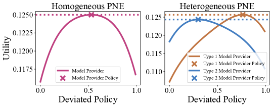
Figure 1: Utility of a single model provider with a deviated policy for both homogeneous and heterogeneous PNE in the configuration of Ex. 5.2.

As shown in Fig. 1, we plot each player’s utility if they deviate to a different policy. From the figure, it is evident that no player benefits from deviating, thereby verifying the correctness of the PNEs.

6 Synthetic Experiments

In this section, we conduct synthetic experiments to investigate how the temperature parameter $t$ in the probability choice model (Eq. 3) influences the existence of homogeneous and heterogeneous PNEs in HD-Game-Probability.

Data-generating processes.

Because our theoretical results do not depend on the number of data sources $K$, we set $K=2$ for simplicity. We also choose $D=2$ to fulfill Assump. 4.1. We randomly generate 10 game configurations with different $\{\Sigma_{k},\beta_{k},w_{k}\}_{k\in[K]}$. Each covariance matrix is constructed so that its largest eigenvalue does not exceed 1. In addition, we set $w_{2}\geq 0.1$ to avoid a scenario where the first data source fully dominates the market. The number of model providers $N$ is varied from $\{2,3,4,\dots,30\}$ to explore the effect of $N$ on the critical values of $t$.

Calculating critical temperature parameters.

Following Prop. 4.1, each model provider $n$’s strategy $\hat{\theta}_{n}$ must take the form $\bar{\theta}(\boldsymbol{q}_{n})$ with $\boldsymbol{q}_{n}\in\Delta_{2}$ and $\boldsymbol{q}_{n}=(\alpha_{n},1-\alpha_{n})$ for $0\leq\alpha_{n}\leq 1$. To verify whether a candidate strategy profile $\hat{\boldsymbol{\theta}}$ is a PNE, we enumerate all possible deviations: for each provider $n$, we check every $\alpha_{n}\in\{0,0.002,0.004,\dots,0.998,1\}$ to see if a profitable deviation exists. Using this enumeration, we identify:

• Homogeneous PNE. We seek the threshold $\underline{t}$ given in Thms. 5.2 and 5.6. Specifically, we search over $\underline{t}\in\{0.001,0.002,\dots,0.999,1\}\times(2\ell_{\max})$ to find the minimal $t$ for which the strategy profile $\hat{\boldsymbol{\theta}}^{\text{Homo}}$ (from Thm. 5.6) is indeed a PNE.

• Heterogeneous PNE. We seek the maximal $t$ for which a heterogeneous PNE exists. Since determining the exact maximum can be complex in game theory (Gottlob et al., 2003; Fabrikant et al., 2004), we adopt an empirical procedure inspired by the proof of Thm. 5.7. For each candidate $t$, we use Alg. 2 (discussed in App. B) to obtain a heterogeneous PNE candidate, then apply the same enumeration technique to verify whether it is a PNE. We thus find the largest $t$ in $\{0.001,0.002,\dots,0.999,1\}\times(2\ell_{\max})$ for which our approach can produce a heterogeneous PNE. Although this does not guarantee the true maximum, it provides a useful lower bound.

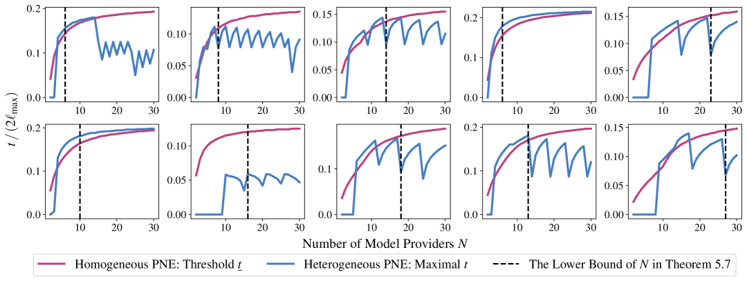
Figure 2: In the probability choice model, this figure reports, across 10 randomly generated games, the threshold $\underline{t}$ that guarantees the existence of a homogeneous PNE and the approximate largest value of $t$ that guarantees the existence of a heterogeneous PNE, as $N$ varies.

Results and analysis.

Fig. 2 presents our experimental results. We make the following observations:

1. Homogeneous PNE. The threshold temperature $\underline{t}$ given in Thms. 5.2 and 5.6 generally increases with $N$, but the growth curve flattens for larger $N$. This is consistent with Thms. 5.2 and 5.6, which guarantee that $\underline{t}\leq 2\ell_{\max}$ and thus ensure the existence of a homogeneous PNE once $t\geq 2\ell_{\max}$, independent of $N$. Moreover, in our setups, the minimal $t$ is often significantly less than $2\ell_{\max}$ (roughly $0.1\times(2\ell_{\max})$ to $0.2\times(2\ell_{\max})$).

2. Heterogeneous PNE. Our empirical approach effectively finds heterogeneous PNEs once $N$ exceeds the lower bound given in Thm. 5.7. Nonetheless, because the conditions in Thm. 5.7 are sufficient but not necessary, we observe that a heterogeneous PNE can exist even when $N$ is smaller than that bound. The curve for the heterogeneous PNE is not smooth and exhibits periodic fluctuations. This is due to the fact that the heterogeneous PNE in HD-Game-Probability depends on the PNE in the corresponding HD-Game-Proximity, which itself has a non-smooth dependence on $N$ (Thms. 5.4 and 5.5).

3. Coexistence of homogeneous and heterogeneous PNE. In some games, the heterogeneous PNE curve appears above the homogeneous PNE curve, suggesting that both types may coexist. However, in other cases (e.g., the second row and second column of Fig. 2), no such coexistence is observed. In addition, as $N$ increases, the maximal $t$ required for a heterogeneous PNE tends to be lower than the threshold $\underline{t}$ required for a homogeneous PNE, indicating that the coexistence of both PNE types becomes increasingly unlikely for large $N$.

7 Conclusions

We propose the Heterogeneous Data Game to analyze competition among ML models in heterogeneous data markets. By studying PNE under proximity and probability choice models, we derive conditions for the existence of different PNE types, showing key factors that shape competitive ML marketplaces.

Impact Statement

This work presents a game-theoretic framework to study competition among ML providers across heterogeneous data sources. By analyzing market equilibrium, it offers insights for designing policies that promote fair and diverse model offerings. Without such safeguards, smaller or less profitable data sources may be neglected, exacerbating inequalities. We aim for our findings to guide policymakers and stakeholders in shaping responsible and equitable ML marketplaces.

Appendix A Omitted Examples

Example A.1.

Let $N=K=3$ with $\theta_{1}=(0,0,1)$, $\theta_{2}=(2,0,1)$, and $\theta_{3}=(0,1,1)$. The covariance matrices are $\Sigma_{1}=\Sigma_{2}=\Sigma_{3}=I$, and the weights are given by $\boldsymbol{w}=(w_{1},w_{2},w_{3})=(0.6,0.25,0.15)$. A graphical explanation is provided in Fig. 3, where $\theta_{1}$, $\theta_{2}$, and $\theta_{3}$ correspond to the vertices A, B, and C of the triangle, respectively.

Figure 3: The graphical explanation of Ex. A.1.

In this case, the Mahalanobis distance reduces to the standard Euclidean distance. It is straightforward to verify that, at a PNE, two players will choose strategy $\theta_{1}$, while the remaining player will adopt a strategy along the segment DE within the triangle (D and E satisfy that BA = BE and CA = CD), excluding the vertices D and E.

Appendix B An Approach to Find a Potential Heterogeneous PNE in HD-Game-Probability

B.1 Approach Design

We first define the following mapping $\mathcal{M}$ from $\Delta_{K}^{N}=\underbrace{\Delta_{K}\times\cdots\times\Delta_{K}}_{N\text{ times}}$ to $\Delta_{K}^{N}$. For a $(\boldsymbol{q}_{1},\boldsymbol{q}_{2},\dots,\boldsymbol{q}_{N})\in\Delta_{K}^{N}$, $\mathcal{M}(\boldsymbol{q}_{1},\boldsymbol{q}_{2},\dots,\boldsymbol{q}_{N})$ is calculated through Alg. 1.

Algorithm 1 The $\mathcal{M}$ mapping from $\Delta_{K}^{N}$ to $\Delta_{K}^{N}$

1:Input: $\boldsymbol{q}_{1},\boldsymbol{q}_{2},\dots,\boldsymbol{q}_{N}\in\Delta_{K}$

2:$\hat{\theta}_{n}\leftarrow\bar{\theta}(\boldsymbol{q}_{n})$ for all $n\in[N]$

3:$\ell_{n,k}\leftarrow d_{M}^{2}(\hat{\theta}_{n},\theta_{k};\Sigma_{k}^{-1})=(\hat{\theta}_{n}-\theta_{k})^{\top}\Sigma_{k}(\hat{\theta}_{n}-\theta_{k})$ for all $n\in[N]$ and $k\in[K]$

4:$p_{n,k}\leftarrow\exp(-\ell_{n,k}/t)/(\sum_{i=1}^{N}\exp(-\ell_{i,k}/t))$ for all $n\in[N]$ and $k\in[K]$

5:$\tilde{q}_{n,k}\leftarrow w_{k}p_{n,k}(1-p_{n,k})/(\sum_{j=1}^{K}w_{j}p_{n,j}(1-p_{n,j}))$ for all $n\in[N]$ and $k\in[K]$

6:$\tilde{\boldsymbol{q}}_{n}\leftarrow(\tilde{q}_{n,1},\dots,\tilde{q}_{n,K})$ for all $n\in[N]$

7:Output: $(\tilde{\boldsymbol{q}}_{1},\tilde{\boldsymbol{q}}_{2},\dots,\tilde{\boldsymbol{q}}_{N})$

We also need the following definition.

Definition B.1 ($k_{n}$).

Given a PNE $\hat{\boldsymbol{\theta}}^{\text{Hete}}$ in HD-Game-Proximity, define $k_{n}$ as follows.

$$k_{n}\triangleq\left(\text{the index }k\text{ such that }\theta_{k}=\hat{\theta}^{\text{Prox}}_{n}\right).$$

Based on the mapping $\mathcal{M}$ and the constant $k_{n}$, the pseudocode of our approach is provided in Alg. 2. The approach consists of several steps. First, we compute the PNE $\hat{\boldsymbol{\theta}}^{\text{Prox}}$ of the corresponding HD-Game-Proximity using Thms. 5.4 and 5.5. Then, starting from this strategy profile, we find a fixed point of the mapping $\mathcal{M}$ defined in Alg. 1. Once a fixed point is identified, we output the corresponding strategy profile $\hat{\boldsymbol{\theta}}=(\hat{\theta}_{1},\dots,\hat{\theta}_{N})$, where each $\hat{\boldsymbol{\theta}}_{n}=\bar{\theta}(\boldsymbol{q}_{n})$.

Algorithm 2 An Approach to Find a Potential Heterogeneous PNE in HD-Game-Probability

1:Input: Game parameters $\{\Sigma_{k},\theta_{k},w_{k}\}_{k\in[K]}$ and $N$

2:Calculate the PNE $\hat{\boldsymbol{\theta}}^{\text{Prox}}$ based on Thms. 5.4 and 5.5 in HD-Game-Proximity

3:Calculate $k_{n}$ for all $n\in[N]$ based on Def. B.1

4:$\boldsymbol{q}_{n}\leftarrow\underbrace{\left(0,0,\dots,1,0,\dots,0\right)}_{\text{the }k_{n}\text{-th element is }1}$

5:while Not convergent do

6:  $(\boldsymbol{q}_{1},\boldsymbol{q}_{2},\dots,\boldsymbol{q}_{N})\leftarrow\mathcal{M}(\boldsymbol{q}_{1},\boldsymbol{q}_{2},\dots,\boldsymbol{q}_{N})$ given in Alg. 1

7:end while

8:$\hat{\theta}^{\text{Hete}}_{n}\leftarrow\bar{\theta}(\boldsymbol{q}_{n})$ for all $n\in[N]$

9:$\hat{\boldsymbol{\theta}}^{\text{Hete}}\leftarrow(\hat{\theta}^{\text{Hete}}_{1},\dots,\hat{\theta}^{\text{Hete}}_{N})$

10:Output: $\hat{\boldsymbol{\theta}}^{\text{Hete}}$

B.2 The Idea of the Approach

Let $\bar{C}$ be the constant that only depends on $\{\Sigma_{k},\theta_{k},w_{k}\}_{k=1}^{K}$ in Lem. C.8. For any $t>0$ and $\beta\geq 1$, define the space

$$\mathcal{Q}^{(t,\beta)}\triangleq\mathcal{Q}^{(t,\beta)}_{1}\times\mathcal{Q}^{(t,\beta)}_{2}\times\dots\times\mathcal{Q}^{(t,\beta)}_{N}$$ (13)

where

$$\mathcal{Q}^{(t,\beta)}_{n}\triangleq\left\{\boldsymbol{q}\in\Delta_{K}:\left\|\boldsymbol{q}-\underbrace{\left(0,0,\dots,1,0,\dots,0\right)}_{\text{the }k_{n}\text{-th element is }1}\right\|_{\infty}\leq t^{\beta}/\bar{C}\right\}.$$

Based on the above definition, we could provide two important properties of the mapping $\mathcal{M}$.

1. (Lem. C.19) For any $(\boldsymbol{q}_{1},\dots,\boldsymbol{q}_{N})\in\Delta_{K}^{N}$, let $\hat{\boldsymbol{\theta}}=(\hat{\theta}_{1},\hat{\theta}_{2},\dots,\hat{\theta}_{N})$ where $\hat{\theta}_{n}=\bar{\theta}(\boldsymbol{q}_{n})$, $\forall n\in[N]$. If $(\boldsymbol{q}_{1},\dots,\boldsymbol{q}_{N})$ is a fixed point of the mapping $\mathcal{M}$, then for all $n\in[N]$,

   $$\left.\frac{\partial u_{n}(\theta,\hat{\boldsymbol{\theta}}_{-n})}{\partial\theta}\right|_{\theta=\hat{\theta}_{n}}=0.$$

2. (Lem. C.22) When $\beta>1$, there exists a constant $\underline{t}$, depending only on $\{\Sigma_{k},\theta_{k},w_{k}\}_{k=1}^{K}$ and $\beta$, such that when $t\leq\underline{t}$, for any $(\boldsymbol{q}_{1},\boldsymbol{q}_{2},\dots,\boldsymbol{q}_{N})\in\mathcal{Q}^{(t,\beta)}$ defined in Eq. 13, then $\mathcal{M}(\boldsymbol{q}_{1},\boldsymbol{q}_{2},\dots,\boldsymbol{q}_{N})\in\mathcal{Q}^{(t,\beta)}$.

Based on the Brouwer fixed-point theorem, the second point (Lem. C.22) guarantees the existence of a fixed point $(\boldsymbol{q}_{1},\dots,\boldsymbol{q}_{N})\in\mathcal{Q}^{(t,\beta)}$ for the mapping $\mathcal{M}$. Consequently, by the first point (Lem. C.19), the corresponding strategy profile $\hat{\boldsymbol{\theta}}^{\text{Hete}}=(\hat{\theta}^{\text{Hete}}_{1},\dots,\hat{\theta}^{\text{Hete}}_{N})$, where each $\hat{\boldsymbol{\theta}}^{\text{Hete}}_{n}=\bar{\theta}(\boldsymbol{q}_{n})$, satisfies the zero partial gradient condition at $\hat{\theta}^{\text{Hete}}_{n}$ for $u_{n}(\theta,\hat{\boldsymbol{\theta}}^{\text{Hete}}_{-n})$ for all $n\in[N]$, which is a necessary condition for a PNE. Therefore, $\hat{\boldsymbol{\theta}}^{\text{Hete}}$ serves as a candidate for a heterogeneous PNE in HD-Game-Probability.

Appendix C Omitted Proofs

Additional notations.

For any two vectors $\boldsymbol{x}=(x_{1},\dots,x_{M})\in\mathbb{R}^{M}$ and $\boldsymbol{y}=(y_{1},\dots,y_{M})\in\mathbb{R}^{M}$, we say $\boldsymbol{x}$ is dominated by $\boldsymbol{y}$ if for all $i\in[M]$, $y_{i}\leq x_{i}$ and there exists a $j\in[M]$, $y_{j}<x_{j}$.

C.1 Proof of Prop. 4.1

We first prove Eq. 7.

Proof of Eq. 7.

According to the definition of the Mahalanobis distance, we have

$$\bar{\theta}(\boldsymbol{q})=\operatorname*{arg\,min}_{\theta}\sum_{k=1}^{K}q_{k}d_{M}^{2}(\theta,\theta_{k};\Sigma_{k}^{-1})=\operatorname*{arg\,min}_{\theta}\sum_{k=1}^{K}q_{k}(\theta-\theta_{k})^{T}\Sigma_{k}(\theta-\theta_{k})$$

Denote the part in $\operatorname*{arg\,min}$ in the right-hand side of the above equation as $L(\theta)$. And since $\boldsymbol{q}\in\Delta_{K}$ and $\Sigma_{k}\succ 0$, we have

$$\nabla L(\theta)=2\sum_{k=1}^{K}q_{k}\Sigma_{k}(\theta-\theta_{k}),\quad\nabla^{2}L(\theta)=2\sum_{k=1}^{K}q_{k}\Sigma_{k}\succ 0.$$

As a result, $L(\theta)$ is strictly convex and it has the unique minimizer $\bar{\theta}(\boldsymbol{q})$. In addition, $\bar{\theta}(\boldsymbol{q})$ must satisfy that $\nabla L(\bar{\theta}(\boldsymbol{q}))=0$, which means

$$2\sum_{k=1}^{K}q_{k}\Sigma_{k}(\bar{\theta}(\boldsymbol{q})-\theta_{k})=0.$$

As a result,

$$\bar{\theta}(\boldsymbol{q})=\left(\sum_{k=1}^{K}q_{k}\Sigma_{k}\right)^{-1}\left(\sum_{k=1}^{K}q_{k}\Sigma_{k}\theta_{k}\right).$$

Now the claim follows. ∎

For the proof of Prop. 4.1, we first introduce the following lemma.

Lemma C.1.

Let $\vartheta$ be defined in Eq. 6. Then for any $\theta\not\in\vartheta$, there exists a $\theta^{*}\in\vartheta$ such that for all $k\in[K]$, $d_{M}(\theta^{*},\theta_{k};\Sigma_{k}^{-1})<d_{M}(\theta,\theta_{k};\Sigma_{k}^{-1})$.

Proof of Lem. C.1.

Define the following function $f:\mathbb{R}^{D}\rightarrow\mathbb{R}^{K}$ as

$$f(\theta)=\left(d_{M}^{2}(\theta,\theta_{1};\Sigma_{1}^{-1}),d_{M}^{2}(\theta,\theta_{2};\Sigma_{2}^{-1}),\dots,d_{M}^{2}(\theta,\theta_{K};\Sigma_{K}^{-1})\right).$$

For any $k\in[K]$, define $f_{k}(\theta)=d_{M}^{2}(\theta,\theta_{k};\Sigma_{k}^{-1})$. Note that for any $k\in[K]$, since $\Sigma_{k}\succ 0$, we have $d_{M}^{2}(\theta,\theta_{k};\Sigma_{k}^{-1})=(\theta-\theta_{k})^{\top}\Sigma_{k}(\theta-\theta_{k})$ is convex w.r.t. $\theta$. As a result, according to Boyd [2004], for every Pareto optimal point $\theta$ of $f$, there is some $\boldsymbol{q}\in\Delta_{K}$ such that

$$\theta=\operatorname*{arg\,min}_{\theta^{\prime}}\sum_{k=1}^{K}q_{k}d_{M}^{2}(\theta^{\prime},\theta_{k};\Sigma_{k}^{-1})=\bar{\theta}(\boldsymbol{q}).$$

Hence, the set $\vartheta$ defined in Eq. 6 contains all Pareto optimal points.

Furthermore, for any points $\theta\not\in\vartheta$, there must exist a $\theta^{\prime}\in\vartheta$ such that $f(\theta^{\prime})$ dominates $f(\theta)$ [Ehrgott, 2005], which proves the claim. ∎

Now we could prove Prop. 4.1.

proof of Prop. 4.1.

(1) In the proximity model, let $\hat{\boldsymbol{\theta}}=(\hat{\theta}_{1},\hat{\theta}_{2},\dots,\hat{\theta}_{K})$ be a PNE. If $\hat{\theta}_{k}\in\vartheta,\forall k\in[K]$, then the claim is already satisfied. Now suppose there exists an index $n$ such that $\hat{\theta}_{n}\not\in\vartheta$. According to Lem. C.1, there exists a policy $\theta^{\prime}\in\vartheta$ such that $\forall k\in[K],\ell^{\prime}_{n,k}=d_{M}^{2}(\theta^{\prime},\theta_{k};\Sigma_{k}^{-1})<d_{M}^{2}(\hat{\theta}_{n},\theta_{k};\Sigma_{k}^{-1})=\ell_{n,k}$. Consider the new strategy profile $\tilde{\boldsymbol{\theta}}=(\theta^{\prime},\hat{\boldsymbol{\theta}}_{-n})$. We now show that $\tilde{\boldsymbol{\theta}}$ is also a PNE.

Since $g^{\text{PROX}}_{n}$ is decreasing on the $n$-th element and $\hat{\boldsymbol{\theta}}$ is a PNE, we have that

$$u_{n}(\hat{\boldsymbol{\theta}})=\sum_{k=1}^{K}w_{k}g^{\text{PROX}}_{n}(\ell_{1,k},\dots,\ell_{N,k})\leq\sum_{k=1}^{K}w_{k}g^{\text{PROX}}_{n}(\ell_{1,k},\dots,\ell_{n-1,k},\ell^{\prime}_{n,k},\ell_{n+1,k},\dots,\ell_{N,k})=u_{n}(\tilde{\boldsymbol{\theta}})\leq u_{n}(\hat{\boldsymbol{\theta}}).$$

As a result, $u_{n}(\tilde{\boldsymbol{\theta}})=u_{n}(\hat{\boldsymbol{\theta}})$ and player $n$ will not benefit by deviation. Furthermore, $\forall k\in[K]$, we have $g^{\text{PROX}}_{n}(\ell_{1,k},\dots,\ell_{N,k})=g^{\text{PROX}}_{n}(\ell_{1,k},\dots,\ell_{n-1,k},\ell^{\prime}_{n,k},\ell_{n+1,k},\dots,\ell_{N,k})$. (Otherwise, player $n$ would benefit by deviation.) Since $\ell^{\prime}_{n,k}<\ell_{n,k}$, we have

$$g^{\text{PROX}}_{n}(\ell_{1,k},\dots,\ell_{N,k})=g^{\text{PROX}}_{n}(\ell_{1,k},\dots,\ell_{n-1,k},\ell^{\prime}_{n,k},\ell_{n+1,k},\dots,\ell_{N,k})=0$$

and hence $\ell_{n,k}>\ell^{\prime}_{n,k}>\min_{i\in[N]}\ell_{i,k},\forall k\in[K]$. As a result, this deviation will not affect any other players’ utility. Specifically, consider any other player $j\in[N]\backslash\{n\}$. We have

$$g^{\text{PROX}}_{j}(\ell_{1,k},\dots,\ell_{n-1,k},\ell^{\prime}_{n,k},\ell_{n+1,k},\dots,\ell_{N,k})=g^{\text{PROX}}_{j}(\ell_{1,k},\dots,\ell_{N,k}).$$ (14)

Furthermore, since $\ell^{\prime}_{n,k}<\ell_{n,k}$, we have that for any $\theta^{\prime\prime}\in\mathbb{R}^{D}$ and $\ell^{\prime\prime}_{j,k}=d_{M}^{2}(\theta^{\prime\prime},\theta_{k};\Sigma_{k}^{-1})$, we have $\forall j\in[N]$,

$$\,g^{\text{PROX}}_{j}(\ell_{1,k},\dots,\ell_{j-1,k},\ell^{\prime\prime}_{j,k},\ell_{j+1,k},\dots,\ell_{n-1,k},\ell^{\prime}_{n,k},\ell_{n+1,k},\dots,\ell_{N,k})$$ (15)

$$\leq \,g^{\text{PROX}}_{j}(\ell_{1,k},\dots,\ell_{j-1,k},\ell^{\prime\prime}_{j,k},\ell_{j+1,k},\dots,\ell_{N,k}).$$

As a result,

$$\,u_{j}((\theta^{\prime\prime},\tilde{\boldsymbol{\theta}}_{-j}))$$

$$= \,\sum_{k=1}^{K}w_{k}\cdot g^{\text{PROX}}_{j}(\ell_{1,k},\dots,\ell_{j-1,k},\ell^{\prime\prime}_{j,k},\ell_{j+1,k},\dots,\ell_{n-1,k},\ell^{\prime}_{n,k},\ell_{n+1,k},\dots,\ell_{N,k})$$

$$\leq \,\sum_{k=1}^{K}w_{k}\cdot g^{\text{PROX}}_{j}(\ell_{1,k},\dots,\ell_{j-1,k},\ell^{\prime\prime}_{j,k},\ell_{j+1,k},\dots,\ell_{N,k})$$ (by Eq. 15)

$$\leq \,\sum_{k=1}^{K}w_{k}\cdot g^{\text{PROX}}_{j}(\ell_{1,k},\dots,\ell_{j-1,k},\ell_{j,k},\ell_{j+1,k},\dots,\ell_{N,k}) \hat{\boldsymbol{\theta}} u_{j}(\hat{\boldsymbol{\theta}})\geq u_{j}(\theta^{\prime\prime},\hat{\boldsymbol{\theta}}_{-j})$$ ( is a PNE and hence )

$$= \,\sum_{k=1}^{K}w_{k}\cdot g^{\text{PROX}}_{j}(\ell_{1,k},\dots,\ell_{n-1,k},\ell^{\prime}_{n,k},\ell_{n+1,k},\dots,\ell_{N,k})$$ (by Eq. 14)

$$= \,u_{j}(\tilde{\boldsymbol{\theta}}).$$

Therefore, any player will not benefit by deviation from $\tilde{\boldsymbol{\theta}}$ and $\tilde{\boldsymbol{\theta}}$ is a PNE.

To prove the original claim, we can keep this procedure. After at most $N$ steps, we can get a new PNE $\boldsymbol{\theta}^{*}=(\theta^{*}_{1},\dots,\theta^{*}_{N})$ from $\boldsymbol{\theta}$ and $\theta^{*}_{k}\in\vartheta,\forall k\in[K]$. Now the claim follows.

(2) In the probability model, suppose there exists a PNE $\boldsymbol{\theta}=(\theta_{1},\theta_{2},\dots,\theta_{N})$ and an index $n\in[N]$ such that $\theta_{n}\not\in\vartheta$. Then according to Lem. C.1, there exists $\theta^{\prime}\in\vartheta$ such that $\forall k\in[K],d_{M}(\theta^{\prime},\theta_{k};\Sigma_{k}^{-1})<d_{M}(\theta_{n},\theta_{k};\Sigma_{k}^{-1})$. Since $g^{\text{PROP}}_{n}$ is strictly decreasing on the $n$-th element, we could conclude that player $n$ will benefit if deviating to the policy $\theta^{\prime}$, which leads to a contradiction. Now the claim follows. ∎

C.2 Proof of Thm. 5.1

We first introduce the following lemma.

Lemma C.2.

Suppose that Assump. 4.1 holds. Let $\boldsymbol{q}\in\Delta_{K}$ and $\theta=\bar{\theta}(\boldsymbol{q})$. Then for any $k_{0}\in[K]$ such that $q_{k_{0}}>0$, there exists a strategy $\tilde{\theta}\in\vartheta$ such that

$$\forall k\in[K]\backslash\{k_{0}\},\quad d_{M}(\tilde{\theta},\theta_{k};\Sigma_{k}^{-1})<d_{M}(\theta,\theta_{k};\Sigma_{k}^{-1}).$$

Proof.

For any $k\in[K]\backslash\{k_{0}\}$, define $v_{k}=\Sigma_{k}(\theta-\theta_{k})$. Furthermore, define the following matrix

$$A=\begin{pmatrix}v_{1}&v_{2}&\dots&v_{k_{0}-1}&v_{k_{0}+1}&\dots v_{K}.\end{pmatrix}$$

Then for any $\boldsymbol{y}\in\mathbb{R}^{K-1}$ such that $\boldsymbol{y}\geq 0$ and $\boldsymbol{y}\neq 0$, we must have $A\boldsymbol{y}\neq 0$. Otherwise, we can construct a new $\boldsymbol{q}^{\prime}$ such that

$$q^{\prime}_{k}=\begin{cases}y_{k}/\left(\sum_{k^{\prime}=1}^{K-1}y_{k^{\prime}}\right)&\text{if }k<k_{0},\\ 0&\text{if }k=k_{0},\\ y_{k-1}/\left(\sum_{k^{\prime}=1}^{K-1}y_{k^{\prime}}\right)&\text{if }k>k_{0}.\end{cases}$$

As a result,

$$\sum_{k=1}^{K}q_{k}^{\prime}\Sigma_{k}(\theta-\theta_{k})=\sum_{k=1}^{K}q_{k}^{\prime}v_{k}=A\boldsymbol{y}/\left(\sum_{k^{\prime}=1}^{K-1}y_{k^{\prime}}\right)=0$$

and $\theta=\bar{\theta}(\boldsymbol{q}^{\prime})=\bar{\theta}(\boldsymbol{q})$, which violates Assump. 4.1.

According to Gordan’s theorem (Lem. D.1, [Mangasarian, 1994]), there must exist a vector $x\in\mathbb{R}^{D}$ such that $(-A)^{\top}x>0$, which means for all $k\in[K]\backslash\{k_{0}\}$, we have $v_{k}^{\top}x<0$. Now construct the following $\theta^{\prime}_{t}=\theta+t\cdot x$ with any $t\geq 0$. We can get that, for any $k\in[K]\backslash\{k_{0}\}$,

$$\left.\frac{\mathrm{d}d_{M}^{2}(\theta^{\prime}_{t},\theta_{k};\Sigma_{k}^{-1})}{\mathrm{d}t}\right|_{t=0} =\left.\frac{\mathrm{d}\left(\theta+t\cdot x-\theta_{k}\right)^{\top}\Sigma_{k}\left(\theta+t\cdot x-\theta_{k}\right)}{\mathrm{d}t}\right|_{t=0}=\left.2x^{\top}\Sigma_{k}(\theta+t\cdot x-\theta_{k})\right|_{t=0}$$

$$=2x^{\top}\Sigma_{k}(\theta-\theta_{k})=2x^{\top}v_{k}<0.$$

As a result, there must exist a $t_{k}>0$ such that for any $0<t<t_{k}$, we have $d_{M}^{2}(\theta^{\prime}_{t},\theta_{k};\Sigma_{k}^{-1})<d_{M}^{2}(\theta,\theta_{k};\Sigma_{k}^{-1})$. Now choose $t^{\prime}=\min\{t_{1},t_{2},\dots,t_{k_{0}-1},t_{k_{0}+1},\dots,t_{K}\}/2$ and let $\theta^{\prime}=\theta+t^{\prime}\cdot x$. Then for all $k\in[K]\backslash\{k_{0}\}$, we must have $d_{M}(\theta^{\prime},\theta_{k};\Sigma_{k}^{-1})<d_{M}(\theta,\theta_{k};\Sigma_{k}^{-1})$.

Now if $\theta^{\prime}\in\vartheta$, the claim has already follows. When $\theta^{\prime}\not\in\vartheta$, according to the proof of Lem. C.1 (see Sec. C.1), $\vartheta$ contains all Pareto optimal points. As a result, there must exist a strategy $\tilde{\theta}\in\vartheta$ such that for all $k\in[K]\backslash\{k_{0}\},d_{M}(\tilde{\theta},\theta_{k};\Sigma_{k}^{-1})<d_{M}(\theta^{\prime},\theta_{k};\Sigma_{k}^{-1})<d_{M}(\theta,\theta_{k};\Sigma_{k}^{-1})$. Now the claim follows. ∎

Then we could prove Thm. 5.1.

Proof of Thm. 5.1.

(1) We first consider the case where $w_{1}<0.5$. Suppose a PNE $\hat{\boldsymbol{\theta}}=(\hat{\theta}_{1},\hat{\theta}_{2})$ exists. According to Prop. 4.1, we can assume that $\hat{\theta}_{1},\hat{\theta}_{2}\in\vartheta$. Since the sum of the utilities of two players is $1$, there must exist one player that has utility not greater than $0.5$. Without loss of generality, we assume that $u_{1}(\hat{\boldsymbol{\theta}})\leq 0.5$ and $u_{2}(\hat{\boldsymbol{\theta}})\geq 0.5$. Now we construct a new policy $\theta^{\prime}$ for player $1$ such that $u_{1}(\theta^{\prime},\hat{\theta}_{2})>0.5$.

According to Assump. 4.1, there exists a unique $\boldsymbol{q}\in\Delta_{K}$ such that $\hat{\theta}_{2}=\bar{\theta}(\boldsymbol{q})$. Since $\boldsymbol{q}\in\Delta_{K}$, there must exist one element $k_{0}$ such that $q_{k_{0}}>0$. According to Lem. C.2, there must exist a $\theta^{\prime}\in\vartheta$ such that

$$\forall k\in[K]\backslash\{k_{0}\},\quad d_{M}(\theta^{\prime},\theta_{k};\Sigma_{k}^{-1})<d_{M}(\theta,\theta_{k};\Sigma_{k}^{-1}).$$

Now by the proximity model as shown in Eq. 2, we have that

$$u_{1}(\theta^{\prime},\hat{\theta}_{2})\geq\sum_{k\in[K]\backslash\{k_{0}\}}w_{k}=1-w_{k_{0}}\geq 1-w_{1}>1-0.5=0.5\geq u_{1}(\hat{\boldsymbol{\theta}}).$$

As a result, $\hat{\boldsymbol{\theta}}$ is not a PNE, which leads to a contradiction.

(2) We then consider the case when $w_{1}\geq 0.5$.

We first show that $\hat{\boldsymbol{\theta}}=(\theta_{1},\theta_{1})$ is a PNE. In this strategy profile, Since two players choose the same strategy $\theta_{1}$, we have $u_{1}(\hat{\boldsymbol{\theta}})=u_{2}(\hat{\boldsymbol{\theta}})=0.5$. In addition, when any player deviate from the strategy $\theta_{1}$, he could have higher loss on data source $1$ and hence could have utility at most $\sum_{k=2}^{K}w_{k}=1-w_{1}\leq 0.5$. As a result, $\hat{\boldsymbol{\theta}}=(\theta_{1},\theta_{1})$ is a PNE.

Furthermore, consider the case when $w_{1}>0.5$. Suppose there exists another PNE $\hat{\boldsymbol{\theta}}^{\prime}=(\hat{\theta}_{1},\hat{\theta}_{2})\neq\hat{\boldsymbol{\theta}}$. We consider the following two cases.

1. Suppose $\hat{\theta}_{1},\hat{\theta}_{2}\neq\theta_{1}$. Since $u_{1}(\hat{\boldsymbol{\theta}}^{\prime})+u_{2}(\hat{\boldsymbol{\theta}}^{\prime})=1$, there exist one player such that his utility is not greater than $0.5$. Without loss of generality, we assume $u_{1}(\hat{\boldsymbol{\theta}}^{\prime})\leq 0.5$. Then if player $1$ choose strategy $\theta_{1}$, he will get utility at least $w_{1}>0.5\geq u_{1}(\hat{\boldsymbol{\theta}}^{\prime})$, which leads to a contradiction.

2. Suppose one player choose $\theta_{1}$ and the other player does not. Without loss of generality, we assume $\hat{\theta}_{1}^{\prime}=\theta_{1}$ and $\hat{\theta}_{2}^{\prime}\neq\theta_{1}$. In this case, $u_{2}(\hat{\boldsymbol{\theta}}^{\prime})\leq\sum_{k=2}^{K}w_{k}=1-w_{1}<0.5$. However, if player $2$ choose strategy $\theta_{1}$, he will have the same strategy with player $1$ and get utility $0.5>u_{2}(\hat{\boldsymbol{\theta}}^{\prime})$, which leads to a contraction.

To conclude, $\hat{\boldsymbol{\theta}}=(\theta_{1},\theta_{1})$ is the unique PNE when $w_{1}>0.5$.

Now the claim follows. ∎

C.3 Proof of Thm. 5.2

Proof.

(1) We first show that, if a PNE exists, the only possible PNE is that both players choose $\bar{\theta}(\boldsymbol{w})$.

Suppose that $\hat{\boldsymbol{\theta}}=(\hat{\theta}_{1},\hat{\theta}_{2})$ is a PNE. According to the definition of PNE, we must have

$$\hat{\theta}_{1}\in\operatorname*{arg\,max}_{\theta}u_{1}(\theta,\hat{\theta}_{2})=\operatorname*{arg\,max}_{\theta}\sum_{k=1}^{K}w_{k}\cdot p_{1,k}(\theta)$$

where

$$p_{1,k}(\theta)=\frac{\exp\left(-\left(\theta-\theta_{k}\right)^{\top}\Sigma_{k}\left(\theta-\theta_{k}\right)/t\right)}{\exp\left(-\left(\theta-\theta_{k}\right)^{\top}\Sigma_{k}\left(\theta-\theta_{k}\right)/t\right)+\exp\left(-\left(\hat{\theta}_{2}-\theta_{k}\right)^{\top}\Sigma_{k}\left(\hat{\theta}_{2}-\theta_{k}\right)/t\right)}.$$

Note that

$$\,\frac{\partial p_{1,k}(\theta)}{\partial\theta}$$

$$= \,\frac{\exp\left(-\left(\theta-\theta_{k}\right)^{\top}\Sigma_{k}\left(\theta-\theta_{k}\right)/t\right)\cdot\exp\left(-\left(\hat{\theta}_{2}-\theta_{k}\right)^{\top}\Sigma_{k}\left(\hat{\theta}_{2}-\theta_{k}\right)/t\right)}{\left(\exp\left(-\left(\theta-\theta_{k}\right)^{\top}\Sigma_{k}\left(\theta-\theta_{k}\right)/t\right)+\exp\left(-\left(\hat{\theta}_{2}-\theta_{k}\right)^{\top}\Sigma_{k}\left(\hat{\theta}_{2}-\theta_{k}\right)/t\right)\right)^{2}}\cdot\left(-\frac{2}{t}\cdot\Sigma_{k}\left(\theta-\theta_{k}\right)\right)$$

$$= \,-\frac{2}{t}\cdot p_{1,k}(\theta)(1-p_{1,k}(\theta))\Sigma_{k}(\theta-\theta_{k}).$$

As a result,

$$\frac{\partial u_{1}(\theta,\hat{\theta}_{2})}{\partial\theta}=\sum_{k=1}^{K}w_{k}\cdot\frac{\partial p_{1,k}(\theta)}{\partial\theta}=-\frac{2}{t}\cdot\sum_{k=1}^{K}w_{k}p_{1,k}(\theta)(1-p_{1,k}(\theta))\Sigma_{k}(\theta-\theta_{k}).$$

Hence,

$$\left.\frac{\partial u_{1}(\theta,\hat{\theta}_{2})}{\partial\theta}\right|_{\theta=\hat{\theta}_{1}}=-\frac{2}{t}\cdot\sum_{k=1}^{K}w_{k}p_{1,k}(\hat{\theta}_{1})(1-p_{1,k}(\hat{\theta}_{1}))\Sigma_{k}(\hat{\theta}_{1}-\theta_{k})=0.$$ (16)

Similarly, we can get that

$$\left.\frac{\partial u_{2}(\hat{\theta}_{1},\theta)}{\partial\theta}\right|_{\theta=\hat{\theta}_{2}}=-\frac{2}{t}\cdot\sum_{k=1}^{K}w_{k}p_{2,k}(\hat{\theta}_{2})(1-p_{2,k}(\hat{\theta}_{2}))\Sigma_{k}(\hat{\theta}_{2}-\theta_{k})=0.$$

where

$$p_{2,k}(\theta)=\frac{\exp\left(-\left(\theta-\theta_{k}\right)^{\top}\Sigma_{k}\left(\theta-\theta_{k}\right)/t\right)}{\exp\left(-\left(\hat{\theta}_{1}-\theta_{k}\right)^{\top}\Sigma_{k}\left(\hat{\theta}_{1}-\theta_{k}\right)/t\right)+\exp\left(-\left(\theta-\theta_{k}\right)^{\top}\Sigma_{k}\left(\theta-\theta_{k}\right)/t\right)}.$$

Note that $p_{1,k}(\hat{\theta}_{1})+p_{2,k}(\hat{\theta}_{2})=1$. As a result,

$$\left.\frac{\partial u_{2}(\theta,\hat{\theta}_{2})}{\partial\theta}\right|_{\theta=\hat{\theta}_{1}} =-\frac{2}{t}\cdot\sum_{k=1}^{K}w_{k}p_{1,k}(\hat{\theta}_{1})(1-p_{1,k}(\hat{\theta}_{1}))\Sigma_{k}(\hat{\theta}_{1}-\theta_{k})=-\frac{2}{t}\cdot\sum_{k=1}^{K}w_{k}p_{1,k}(\hat{\theta}_{1})p_{2,k}(\hat{\theta}_{2})\Sigma_{k}(\hat{\theta}_{1}-\theta_{k})=0.$$

$$\left.\frac{\partial u_{2}(\hat{\theta}_{1},\theta)}{\partial\theta}\right|_{\theta=\hat{\theta}_{2}} =-\frac{2}{t}\cdot\sum_{k=1}^{K}w_{k}p_{2,k}(\hat{\theta}_{2})(1-p_{2,k}(\hat{\theta}_{2}))\Sigma_{k}(\hat{\theta}_{2}-\theta_{k})=-\frac{2}{t}\cdot\sum_{k=1}^{K}w_{k}p_{1,k}(\hat{\theta}_{1})p_{2,k}(\hat{\theta}_{2})\Sigma_{k}(\hat{\theta}_{2}-\theta_{k})=0.$$

Hence,

$$\sum_{k=1}^{K}w_{k}p_{1,k}(\hat{\theta}_{1})p_{2,k}(\hat{\theta}_{2})\Sigma_{k}(\hat{\theta}_{1}-\theta_{k})=0=\sum_{k=1}^{K}w_{k}p_{1,k}(\hat{\theta}_{1})p_{2,k}(\hat{\theta}_{2})\Sigma_{k}(\hat{\theta}_{2}-\theta_{k})$$

and therefore

$$\sum_{k=1}^{K}w_{k}p_{1,k}(\hat{\theta}_{1})p_{2,k}(\hat{\theta}_{2})\Sigma_{k}(\hat{\theta}_{1}-\hat{\theta}_{2})=0.$$

Define matrix $A=\sum_{k=1}^{K}w_{k}p_{1,k}(\hat{\theta}_{1})p_{2,k}(\hat{\theta}_{2})\Sigma_{k}$ and we have $A(\hat{\theta}_{1}-\hat{\theta}_{2})=0$. Note that for all $k\in[K]$, $w_{k},p_{1,k}(\hat{\theta}_{1}),p_{2,k}(\hat{\theta}_{2})>0$ and $\Sigma_{k}\succ 0$. As a result, $A\succ 0$ and we must have $\hat{\theta}_{1}=\hat{\theta}_{2}$. Note that when $\hat{\theta}_{1}=\hat{\theta}_{2}$, $p_{1,k}(\hat{\theta}_{1})=p_{2,k}(\hat{\theta}_{2})=1/2$. Now Eq. 16 becomes

$$-\frac{2}{t}\cdot\sum_{k=1}^{K}w_{k}\cdot\frac{1}{2}\cdot\frac{1}{2}\Sigma_{k}(\hat{\theta}_{1}-\theta_{k})=0.$$

As a result, $\hat{\theta}_{1}=\bar{\theta}(\boldsymbol{w})=\hat{\theta}_{2}$. Hence, if a PNE exists, the only possible PNE is that both players choose $\bar{\theta}(\boldsymbol{w})$.

The claim then follows from the proof of the more general result given by Thm. 5.6 (see Lems. C.3 and C.4 in Sec. C.6 for details).

∎

C.4 Proof of Prop. 5.3

Proof.

Suppose there exists a PNE $\hat{\boldsymbol{\theta}}=(\hat{\theta}_{1},\hat{\theta}_{2},\dots,\hat{\theta}_{N})$ such that there are two players choose the same strategy and the strategy is outside the set $\{\theta_{1},\theta_{2},\dots,\theta_{K}\}$. Without loss of generality, we assume that $\hat{\theta}_{1}=\hat{\theta}_{2}\not\in\{\theta_{1},\dots,\theta_{K}\}$.

Define $\mathcal{K}$ as the set of data sources that player 1 and 2 could get positive utility, i.e.,

$$\mathcal{K}\triangleq\{k:\forall j\in[N],d_{M}(\hat{\theta}_{1},\theta_{k};\Sigma_{k}^{-1})\leq d_{M}(\hat{\theta}_{j},\theta_{k};\Sigma_{k}^{-1})\}.$$

Note that $\mathcal{K}$ cannot be an empty set, as player 1 could otherwise deviate to $\theta_{1}$ and achieve a positive and higher utility. For any $k\in\mathcal{K}$, let

$$k_{n}=\left|\{j:d_{M}(\hat{\theta}_{j},\theta_{k};\Sigma_{k}^{-1})=d_{M}(\hat{\theta}_{1},\theta_{k};\Sigma_{k}^{-1})\}\right|$$

be the number of players that achieve the minimal loss in data source $k$ in the PNE $\hat{\boldsymbol{\theta}}$. Note that $k_{n}\geq 2$ since $\hat{\theta}_{1}=\hat{\theta}_{2}$. Then we can get that

$$u_{1}(\hat{\boldsymbol{\theta}})=u_{2}(\hat{\boldsymbol{\theta}})=\sum_{k\in\mathcal{K}}\frac{w_{k}}{k_{n}}.$$

We consider two cases about $\mathcal{K}$.

1. Consider the case when $|\mathcal{K}|=1$ and $\mathcal{K}=\{k_{0}\}$. If player $1$ deviates to policy $\theta_{k_{0}}$, he will become the only player that has the smallest loss on data source $k$ and hence have a utility at least $w_{k_{0}}>w_{k_{0}}/n_{k_{0}}$, which leads to a contradiction.

2. Consider the case when $|\mathcal{K}|\geq 2$. We further consider two cases about $\hat{\theta}_{1}$.

   1. Consider the case when $\hat{\theta}_{1}\not\in\vartheta$. Then according to the proof of Lem. C.1 (see Sec. C.1), there must exist a $\theta\in\vartheta$ such that for all $k\in[K]$, $d_{M}(\theta,\theta_{k};\Sigma_{k}^{-1})<d_{M}(\hat{\theta}_{2},\theta_{k};\Sigma_{k}^{-1})$. As a result, if player $1$ deviates to the policy $\theta$, he will get utility at least $\sum_{k\in\mathcal{K}}w_{k}>\sum_{k\in\mathcal{K}}w_{k}/k_{n}=u_{1}(\hat{\boldsymbol{\theta}})$, which leads to a contradiction.

   2. Consider the case when $\hat{\theta}_{1}\in\vartheta$. Let $k_{0}$ be the smallest element in $\mathcal{K}$. According to Assump. 4.1, let $\boldsymbol{q}\in\Delta_{K}$ be the unique vector such that $\hat{\theta}_{1}=\bar{\theta}(\boldsymbol{q})$. Since $\hat{\theta}\neq\theta_{k_{0}}$ by assumption, there must exist a $k_{1}\in[K]\backslash\{k_{0}\}$ such that $q_{k_{1}}>0$. Now according to Lem. C.2, there exists a strategy $\theta\in\vartheta$ such that for all $k\in[K]\backslash\{k_{1}\}$, we have $d_{M}(\theta,\theta_{k};\Sigma_{k}^{-1})<d_{M}(\hat{\theta}_{2},\theta_{k};\Sigma_{k}^{-1})$. Let $k_{2}$ be the second smallest element in $\mathcal{K}$. As a result,

      $$u_{1}(\theta,\hat{\boldsymbol{\theta}}_{-1})=\sum_{k\in\mathcal{K}\backslash\{k_{1}\}}w_{k}\geq\sum_{k\in\mathcal{K}\backslash\{k_{2}\}}w_{k}>\frac{w_{k_{0}}}{2}+\frac{w_{k_{2}}}{2}+\sum_{k\in\mathcal{K}\backslash\{k_{0},k_{2}\}}\frac{w_{k}}{k_{n}}\geq u_{1}(\hat{\boldsymbol{\theta}}).$$

      Therefore, player $1$ will have a higher utility if deviating to the policy $\theta$, which leads to a contradiction.

To conclude, all cases lead to a contradiction. As a result, the claim follows. ∎

C.5 Proof of Thm. 5.4

Proof.

(1) We first show the existence of PNE under the condition in Eq. 10.

Note that $z^{*}$ exists since $h(z)\rightarrow\infty$ when $z\rightarrow 0$ and $h(z)=0$ when $z>1$. Moreover, since $h(z)$ is right continuous, it must hold that $h(z^{*})\geq N$. Under the condition in Eq. 10, we have

$$h\left(\frac{w^{\prime}_{k_{0}}}{3}\right)=\sum_{k=1}^{k_{0}}\left\lfloor\frac{3w_{k}^{\prime}}{w^{\prime}_{k_{0}}}\right\rfloor\leq N.$$

In addition, for any $\epsilon>0$, we have

$$h\left(\frac{w^{\prime}_{k_{0}}}{3}+\epsilon\right)=\sum_{k=1}^{k_{0}}\left\lfloor\frac{3w_{k}^{\prime}}{w^{\prime}_{k_{0}}+3\epsilon}\right\rfloor\leq\left(\sum_{k=1}^{k_{0}-1}\left\lfloor\frac{3w_{k}^{\prime}}{w^{\prime}_{k_{0}}+3\epsilon}\right\rfloor\right)+2<\left(\sum_{k=1}^{k_{0}-1}\left\lfloor\frac{3w_{k}^{\prime}}{w^{\prime}_{k_{0}}}\right\rfloor\right)+\left\lfloor\frac{3w_{k_{0}}^{\prime}}{w^{\prime}_{k_{0}}}\right\rfloor\leq N.$$

Hence, it must hold that $z^{*}\leq w^{\prime}_{k_{0}}/3$. Then define

$$\forall k\in[k_{0}],\quad m^{\prime}_{k}=\left\lfloor\frac{w^{\prime}_{k}}{z^{*}}\right\rfloor.$$

As a result, we have that $m^{\prime}_{k}\geq m^{\prime}_{k_{0}}=\left\lfloor w^{\prime}_{k_{0}}/z^{*}\right\rfloor\geq 3$ for all $k\in[k_{0}]$. In addition, due to Eq. 10, by making $\epsilon>0$ small enough, we have that

$$h\left(\sum_{j=k_{0}+1}^{K}w_{j}+\epsilon\right)=\sum_{k=1}^{k_{0}}\left\lfloor\frac{w^{\prime}_{k}}{\left(\sum_{j=k_{0}+1}^{K}w_{j}\right)+\epsilon}\right\rfloor\geq\sum_{k=1}^{k_{0}}\left(\left\lceil\frac{w^{\prime}_{k}}{\left(\sum_{j=k_{0}+1}^{K}w_{j}\right)}\right\rceil-1\right)\geq N.$$

We have that $z^{*}>\sum_{j=k_{0}+1}^{K}w_{j}$.

We construct the PNE based on two cases.

1. Consider the scenario when $h(z^{*})=\sum_{k=1}^{k_{0}}m^{\prime}_{k}=N$. Then let $m^{*}_{k}=m^{\prime}_{k}$ for all $k\in[k_{0}]$.

2. Consider the scenario when $h(z^{*})=\sum_{k=1}^{k_{0}}m^{\prime}_{k}>N$. Note that by the choice of $z^{*}$, $h(z+\epsilon)<N$ for all $\epsilon>0$. Define the set $\mathcal{K}=\{k\in[k_{0}]:w^{\prime}_{k}/z^{*}=m^{\prime}_{k}\}$. As a result, when $\epsilon\rightarrow 0$, $h(z^{*}+\epsilon)=h(z^{*})-|\mathcal{K}|<N$. Hence, it must hold that $|\mathcal{K}|>h(z^{*})-N$. Let $\mathcal{K}^{\prime}$ be the set of the $(h(z^{*})-N)$ smallest elements in $\mathcal{K}$. Define $m^{*}_{k}$ as follows.

   $$\forall k\in[k_{0}],\quad m^{*}_{k}=\begin{cases}m^{\prime}_{k}&\text{if }k\not\in\mathcal{K}^{\prime}\\ m^{\prime}_{k}-1&\text{if }k\in\mathcal{K}^{\prime}.\end{cases}$$ (17)

   Now it holds that $\sum_{k=1}^{k_{0}}m^{*}_{k}=N$.

Construct a strategy profile $\hat{\boldsymbol{\theta}}^{*}=(\hat{\theta}_{1},\hat{\theta}_{2},\dots,\hat{\theta}_{N})$ such that $m^{*}_{1}$ players choose strategy $\theta_{1}$, $m^{*}_{2}$ players choose strategy $\theta_{2}$, $\dots$, and $m^{*}_{k_{0}}$ players choose strategy $\theta_{k_{0}}$. In this profile, for any player that chooses strategy $\theta_{k}$, by the construction of $w^{\prime}_{k}$ in Eq. 11, he will get utility at least $w^{\prime}_{k}/m^{*}_{k}$. Moreover, by the construction of $m^{*}_{k}$ and $m^{\prime}_{k}$, we have that $w^{\prime}_{k}/m^{*}_{k}\geq w^{\prime}_{k}/m^{\prime}_{k}\geq z^{*}$. Hence, all players have a utility at least $z^{*}$. Then we show that for any player $i$ that chooses strategy $\theta_{k}$ with $k\in[k_{0}]$, he could only get utility at most $z^{*}$ by deviation. Consider the two cases of the deviated strategy $\theta^{\prime}$.

1. Consider the case when the deviated strategy $\theta^{\prime}\in\{\theta_{1},\dots,\theta_{k-1},\theta_{k+1},\dots,\theta_{k_{0}}\}$. Suppose the player deviates to strategy $k^{\prime}\neq k$. As a result, the player will utility $w^{\prime}_{k^{\prime}}/(m^{*}_{k^{\prime}}+1)$. When $k^{\prime}\in\mathcal{K}^{\prime}$, we have that $w^{\prime}_{k^{\prime}}/(m^{*}_{k^{\prime}}+1)\leq w^{\prime}_{k^{\prime}}/m^{\prime}_{k^{\prime}}=z^{*}$. When $k^{\prime}\not\in\mathcal{K}^{\prime}$, we have that $w^{\prime}_{k^{\prime}}/(m^{*}_{k^{\prime}}+1)=w^{\prime}_{k^{\prime}}/(m^{\prime}_{k^{\prime}}+1)<z^{*}$. Hence, he could get utility at most $z^{*}$ by deviation.

2. Consider the case when the deviated strategy $\theta^{\prime}\not\in\{\theta_{1},\theta_{2},\dots,\theta_{k_{0}}\}$. Note that $m^{*}_{k}\geq m^{\prime}_{k}-1\geq 2$ by the construction of $m^{*}_{k}$. As a result, for any strategy $\theta_{\tilde{k}}$ with $\tilde{k}\in[k_{0}]$, at least one player chooses it even if player $i$ deviates to $\theta^{\prime}$. As a result, player $i$ could get utility at most $\sum_{k=k_{0}+1}^{K}w_{k}<z^{*}$.

To conclude, in the strategy profile $\hat{\boldsymbol{\theta}}^{*}$, every player obtains a utility of at least $z^{*}$ and can achieve at most $z^{*}$ by deviating. Therefore, $\hat{\boldsymbol{\theta}}^{*}$ is a PNE.

(2) We then show that for any PNE $\hat{\boldsymbol{\theta}}=(\hat{\theta}_{1},\dots,\hat{\theta}_{N})$, we must have $\forall n\in[N],\hat{\theta}_{n}\in\{\theta_{1},\theta_{2},\dots,\theta_{k_{0}}\}$. To prove this claim, we have several steps.

I: We show that for all $k\in[k_{0}]$, there exists $i\in[N]$ such that $\hat{\theta}_{i}=\theta_{k}$. We prove this by contradiction. Suppose that there exists $k\in[k_{0}]$ such that for all $i\in[N]$, $\hat{\theta}_{i}\neq\theta_{k}$. Since the sum of the utilities of all players is $1$, there must exist a player $j$ such that $u_{j}(\hat{\boldsymbol{\theta}})\leq 1/N$. Now let $\theta^{\prime}=\theta_{k}$. Since all other players do not choose $\theta_{k}$, player $j$ could become the only player that achieves the minimal loss on data source $k$. As a result, $u_{j}(\theta^{\prime},\hat{\boldsymbol{\theta}}_{-j})=w_{k}$. Note that

$$w_{k}\cdot N \geq w_{k_{0}}\cdot N\geq\sum_{k=1}^{k_{0}}w_{k_{0}}\cdot\left\lfloor\frac{3w^{\prime}_{k}}{w^{\prime}_{k_{0}}}\right\rfloor$$

$$\geq\sum_{k=1}^{k_{0}}w_{k_{0}}\left(\frac{3w^{\prime}_{k}}{w^{\prime}_{k_{0}}}-1\right)$$

$$\geq\frac{3w_{k_{0}}}{w^{\prime}_{k_{0}}}-k_{0}\cdot w_{k_{0}} \sum_{k=1}^{k_{0}}w^{\prime}_{k}=\sum_{k=1}^{K}w_{k}=1$$ (Because )

$$\geq\frac{3w_{k_{0}}}{w_{k_{0}}+\sum_{k^{\prime}=k_{0}+1}^{K}w_{k^{\prime}}}-k_{0}\cdot w_{k_{0}}$$ (By Eq. 11)

$$\geq\frac{3w_{k_{0}}}{w_{k_{0}}+w_{k_{0}}/3}-k_{0}\cdot w_{k_{0}} w_{k_{0}}>3\sum_{k^{\prime}=k_{0}+1}^{K}w_{k^{\prime}}$$ (By the assumption )

$$\geq\frac{9}{4}-\sum_{k^{\prime}=1}^{k_{0}}w_{k^{\prime}} w_{1}>w_{2}>\dots>w_{K}$$ (Because )

$$\geq\frac{9}{4}-1 \sum_{k=1}^{K}w_{k}=1$$ (Because )

$$=\frac{5}{4}>1.$$

Hence, $w_{k}>1/N$, implying that player $j$ would achieve a higher utility by deviating to strategy $\theta_{k}$, leading to a contradiction.

II: Suppose there exists at least two players $i,j\in[N]$ such that $\hat{\theta}_{i},\hat{\theta}_{j}\not\in\{\theta_{1},\dots,\theta_{k_{0}}\}$. According to the first step, for any $k\in[k_{0}]$, there exists at least one player that choose strategy $k$. As a result, the sum of the utilities of players $i$ and $j$ is at most $\sum_{k=k_{0}+1}^{K}w_{k}$. Hence, at least one player has utility at most $\sum_{k=k_{0}+1}^{K}w_{k}/2$. Without loss of generality, we assume this player is player $i$. Since two players do not choose strategies in $\{\theta_{1},\dots,\theta_{k_{0}}\}$, there must exist a $k^{\prime}\in[k_{0}]$ such that the number of players that choose $\theta_{k^{\prime}}$ is less than $m^{*}_{k}$ (defined in Eq. 17). Hence, if player $i$ deviates to strategy $\theta_{k^{\prime}}$, the utility is at least

$$\frac{w_{k^{\prime}}}{m_{k^{\prime}}}\geq\frac{w^{\prime}_{k^{\prime}}-\sum_{k=k_{0}+1}^{K}w_{k}}{m_{k^{\prime}}}\geq\frac{w^{\prime}_{k^{\prime}}}{m_{k^{\prime}}}-\frac{\sum_{k=k_{0}+1}^{K}w_{k}}{m_{k^{\prime}}}\geq z^{*}-\frac{\sum_{k=k_{0}+1}^{K}w_{k}}{2}>\frac{\sum_{k=k_{0}+1}^{K}w_{k}}{2}.$$

This leads to a contradiction.

III: Suppose there is only one player $i$ that chooses a strategy outside the set $\{\theta_{1},\theta_{2},\dots,\theta_{k_{0}}\}$. The utility of player $i$ is at most $\sum_{k=k_{0}+1}^{K}w_{k}<z^{*}$. In addition, there must exist a $k\in[k_{0}]$ such that in the PNE, at most $m^{*}_{k}-1$ players choose strategy $\theta_{k}$. Therefore, if player $i$ deviates to strategy $\theta_{k}$, he will get utility at least $w^{\prime}_{k}/m^{*}_{k}\geq w^{\prime}_{k}/m^{\prime}_{k}\geq z^{*}$. This leads to a contradiction.

(3) For any PNE $\hat{\boldsymbol{\theta}}$, let $m_{k}=|\{j\in[N]:\hat{\theta}_{j}=\theta_{k}\}|$ be the number of players that choose strategy $\theta_{k}$ in the PNE. We finally show that $|m_{k}-m^{\prime}_{k}|\leq 1$.

Suppose there exists a $k\in[k_{0}]$ such that $|m_{k}-m^{\prime}_{k}|\geq 2$. Consider two cases.

1. Consider the case when $m_{k}-m^{\prime}_{k}\geq 2$. Suppose that a player $i$ chooses strategy $\theta_{k}$. The utility of player $i$ is at most $w^{\prime}_{k}/m_{k}\leq w^{\prime}_{k}/(m^{\prime}_{k}+2)<z^{*}$. Since $\sum_{k=1}^{k_{0}}m_{k}=\sum_{k=1}^{k_{0}}m^{*}_{k}=N$ and $m_{k}\geq m^{\prime}_{k}+2\geq m^{*}_{k}+2$, there must exist a $k^{\prime}\in[k_{0}],k^{\prime}\neq k$ such that $m_{k^{\prime}}<m^{*}_{k^{\prime}}$. As a result, if player $i$ deviates to strategy $\theta_{k^{\prime}}$, he will obtain a utility of at least $w^{\prime}_{k^{\prime}}/(m_{k^{\prime}}+1)\geq w^{\prime}_{k^{\prime}}/m^{*}_{k^{\prime}}\geq w^{\prime}_{k^{\prime}}/m^{\prime}_{k^{\prime}}\geq z^{*}>u_{i}(\hat{\boldsymbol{\theta}})$, which leads to a contradiction.

2. Consider the case when $m^{\prime}_{k}-m_{k}\geq 2$. Since $\sum_{k=1}^{k_{0}}m_{k}=\sum_{k=1}^{k_{0}}m^{*}_{k}=N$ and $m^{*}_{k}\geq m^{\prime}_{k}-1\geq m_{k}+1$, there must exist a $k^{\prime}\in[k_{0}],k^{\prime}\neq k$ such that $m^{*}_{k^{\prime}}<m_{k^{\prime}}$. Let $i$ be any player that chooses strategy $\theta_{k^{\prime}}$ in the PNE. Then $u_{i}(\hat{\boldsymbol{\theta}})=w^{\prime}_{k^{\prime}}/m_{k^{\prime}}\leq w^{\prime}_{k^{\prime}}/(m^{*}_{k^{\prime}}+1)\leq z^{*}$. However, if player $i$ deviates to strategy $\theta_{k}$, he will obtain a utility of at least $w^{\prime}_{k}/(m_{k}+1)\geq w^{\prime}_{k^{\prime}}/(m^{\prime}_{k}-1)>z^{*}$, which leads to a contradiction.

Now the claim follows. ∎

C.6 Proof of Thm. 5.6

We prove Thm. 5.6 by dividing it into three parts.

Lemma C.3.

Under the same assumption as Thm. 5.6, then $\hat{\boldsymbol{\theta}}^{\text{Homo}}=(\hat{\theta}^{\text{M}},\hat{\theta}^{\text{M}},\dots,\hat{\theta}^{\text{M}})$ is a PNE if $t\geq 2\ell_{\max}$.

Lemma C.4.

Under the same assumption as Thm. 5.6, then there exists a constant $\underline{t}$ such that $\hat{\boldsymbol{\theta}}^{\text{Homo}}=(\hat{\theta}^{\text{M}},\hat{\theta}^{\text{M}},\dots,\hat{\theta}^{\text{M}})$ is a PNE if and only if $t\geq\underline{t}$.

Lemma C.5.

Under the same assumption as Thm. 5.6, then there exists a constant $C>0$ such that if $t\geq\max\{6C/N,2\ell_{\max}\}$, then $\hat{\boldsymbol{\theta}}^{\text{Homo}}$ is the unique PNE.

Now Thm. 5.6 follows from Lems. C.3, C.4 and C.5.

C.6.1 Proof of Lem. C.3

Proof.

Since all players choose the same strategy $\hat{\theta}^{\text{M}}$, we focus on analyzing player $1$. We slightly abuse the notation and denote $p_{k}(\theta)$ as follows:

$$p_{k}(\theta)=\frac{\exp\left(-(\theta-\theta_{k})^{\top}\Sigma_{k}(\theta-\theta_{k})/t\right)}{\exp\left(-(\theta-\theta_{k})^{\top}\Sigma_{k}(\theta-\theta_{k})/t\right)+(N-1)\cdot\exp\left(-(\hat{\theta}^{\text{M}}-\theta_{k})^{\top}\Sigma_{k}(\hat{\theta}^{\text{M}}-\theta_{k})/t\right)}.$$

Calculate the gradient and Hessian matrix of $p_{k}(\theta)$ and we get that

$$\nabla p_{k}(\theta) =-\frac{2}{t}\cdot p_{k}(\theta)(1-p_{k}(\theta))\Sigma_{k}(\theta-\theta_{k})$$

$$\nabla^{2}p_{k}(\theta) =\frac{2}{t}p_{k}(\theta)(1-p_{k}(\theta))\Sigma_{k}^{1/2}\left(\frac{2}{t}(1-2p_{k}(\theta))\Sigma_{k}^{1/2}(\theta-\theta_{k})(\theta-\theta_{k})^{\top}\Sigma_{k}^{1/2}-I\right)\Sigma_{k}^{1/2}$$

And we have that

$$u_{1}\left(\theta,\hat{\boldsymbol{\theta}}^{\text{Homo}}_{-1}\right)=\sum_{k=1}^{K}w_{k}p_{k}(\theta),\quad\nabla_{\theta}u_{1}\left(\theta,\hat{\boldsymbol{\theta}}^{\text{Homo}}_{-1}\right)=\sum_{k=1}^{K}w_{k}\nabla p_{k}(\theta),\quad\nabla^{2}_{\theta}u_{1}\left(\theta,\hat{\boldsymbol{\theta}}^{\text{Homo}}_{-1}\right)=\sum_{k=1}^{K}w_{k}\nabla^{2}p_{k}(\theta).$$ (18)

It is easy to verify that, when $\theta=\hat{\theta}^{\text{M}}$, it must hold that $p_{k}(\hat{\theta}^{\text{M}})=1/N$, $u_{1}(\hat{\boldsymbol{\theta}}^{\text{Homo}})=1/N$, and

$$\left.\nabla_{\theta}u_{1}\left(\theta,\hat{\boldsymbol{\theta}}^{\text{Homo}}_{-1}\right)\right|_{\theta=\hat{\theta}^{\text{M}}} =\sum_{k=1}^{K}w_{k}\left(-\frac{2}{t}\right)\cdot\frac{1}{N}\cdot\frac{N-1}{N}\cdot\Sigma_{k}(\hat{\theta}^{\text{M}}-\theta_{k})$$ (19)

$$=-\frac{2(N-1)}{t\cdot N^{2}}\cdot\sum_{k=1}^{K}w_{k}\Sigma_{k}(\bar{\theta}(\boldsymbol{w})-\theta_{k})=0$$

where the last equation is due to the definition of $\bar{\theta}(\boldsymbol{w})$ in Eq. 9.

Define $B=2/t\cdot(1-2p_{k}(\theta))\Sigma_{k}^{1/2}(\theta-\theta_{k})(\theta-\theta_{k})^{\top}\Sigma_{k}^{1/2}$. It must hold that

$$\lambda_{\max}(B)\leq\max\left\{\frac{2}{t}\cdot(1-2p_{k}(\theta))(\theta-\theta_{k})^{\top}\Sigma_{k}(\theta-\theta_{k}),0\right\}\leq\frac{2}{t}\cdot\ell_{\max}.$$

As a result, when $t\geq 2\ell_{\max}$, we have $\lambda_{\max}(B)\leq 1$ and hence $\nabla^{2}p_{k}(\theta)\preceq 0$ and $\nabla^{2}_{\theta}u_{1}(\theta,\hat{\boldsymbol{\theta}}_{-1})\preceq 0$. Therefore, $u_{1}(\theta,\hat{\boldsymbol{\theta}}^{\text{Homo}}_{-1})$ is a concave function when $t\geq 2\ell_{\max}$. Due to Eq. 19, we have $\hat{\theta}^{\text{M}}\in\operatorname*{arg\,max}_{\theta}u_{1}(\theta,\hat{\boldsymbol{\theta}}^{\text{Homo}}_{-1})$. The same results hold for all other players. As a result, $\hat{\boldsymbol{\theta}}^{\text{Homo}}$ is a PNE. ∎

C.6.2 Proof of Lem. C.4

Proof.

Suppose $\hat{\boldsymbol{\theta}}^{\text{Homo}}$ is a PNE when the temperature is $t_{0}^{\prime}$. We slightly abuse the notation and use $p_{1,k}(\theta,t)$ to denote the probability of data source $k$ choosing player $1$ if he deviates to policy $\theta$ in $\hat{\boldsymbol{\theta}}^{\text{Homo}}$ and $u_{1}(\theta,t)$ to denote the corresponding total utility of player $1$. Then

$$p_{1,k}(\theta,t) =\frac{\exp\left(-d_{M}^{2}\left(\theta,\theta_{k};\Sigma_{k}^{-1}\right)/t\right)}{\exp\left(-d_{M}^{2}\left(\theta,\theta_{k};\Sigma_{k}^{-1}\right)/t\right)+(N-1)\exp\left(-d_{M}^{2}\left(\hat{\theta}^{\text{M}},\theta_{k};\Sigma_{k}^{-1}\right)/t\right)}$$

$$=\frac{1}{1+(N-1)\exp\left(\left(d_{M}^{2}\left(\theta,\theta_{k};\Sigma_{k}^{-1}\right)-d_{M}^{2}\left(\hat{\theta}^{\text{M}},\theta_{k};\Sigma_{k}^{-1}\right)\right)/t\right)}$$

$$u_{1}(\theta,t) =\sum_{k=1}^{K}w_{k}p_{1,k}(\theta,t).$$

Fix any $t\geq t_{0}^{\prime}$. Consider any $\theta\in\mathbb{R}^{D}$, define $\alpha=t_{0}^{\prime}/t$ and

$$\theta^{\prime}=\alpha\theta+(1-\alpha)\hat{\theta}^{\text{M}}.$$

Note that $d_{M}^{2}(\cdot,\theta_{k};\Sigma_{k}^{-1})$ is convex, we have that

$$d_{M}^{2}\left(\theta^{\prime},\theta_{k};\Sigma_{k}^{-1}\right)\leq\alpha d_{M}^{2}\left(\theta,\theta_{k};\Sigma_{k}^{-1}\right)+(1-\alpha)d_{M}^{2}\left(\hat{\theta}^{\text{M}},\theta_{k};\Sigma_{k}^{-1}\right).$$

This is equivalent to

$$\frac{d_{M}^{2}\left(\theta,\theta_{k};\Sigma_{k}^{-1}\right)-d_{M}^{2}\left(\hat{\theta}^{\text{M}},\theta_{k};\Sigma_{k}^{-1}\right)}{t}\geq\frac{d_{M}^{2}\left(\theta^{\prime},\theta_{k};\Sigma_{k}^{-1}\right)-d_{M}^{2}\left(\hat{\theta}^{\text{M}},\theta_{k};\Sigma_{k}^{-1}\right)}{t_{0}^{\prime}}.$$

As a result,

$$p_{1,k}(\theta,t) =\frac{1}{1+(N-1)\exp\left(\left(d_{M}^{2}\left(\theta,\theta_{k};\Sigma_{k}^{-1}\right)-d_{M}^{2}\left(\hat{\theta}^{\text{M}},\theta_{k};\Sigma_{k}^{-1}\right)\right)/t\right)}$$

$$\leq\frac{1}{1+(N-1)\exp\left(\left(d_{M}^{2}\left(\theta^{\prime},\theta_{k};\Sigma_{k}^{-1}\right)-d_{M}^{2}\left(\hat{\theta}^{\text{M}},\theta_{k};\Sigma_{k}^{-1}\right)\right)/t_{0}^{\prime}\right)}$$

$$=p_{1,k}(\theta^{\prime},t_{0}^{\prime}).$$

Therefore,

$$u_{1}(\theta,t)=\sum_{k=1}^{K}w_{k}p_{1,k}(\theta,t)\leq\sum_{k=1}^{K}w_{k}p_{1,k}(\theta^{\prime},t_{0}^{\prime})=u_{1}(\theta^{\prime},t_{0}^{\prime})\leq u_{1}(\hat{\theta}^{\text{M}},t_{0}^{\prime})=1/N.$$

Here $u_{1}(\theta^{\prime},t_{0}^{\prime})\leq u_{1}(\hat{\theta}^{\text{M}},t_{0}^{\prime})$ is due to the fact that $\hat{\boldsymbol{\theta}}^{\text{Homo}}$ is a PNE when the temperature is $t_{0}^{\prime}$. Note that $u_{1}(\hat{\theta}^{\text{M}},t)=1/N$ and hence $u_{1}(\hat{\theta}^{\text{M}},t)\geq u_{1}(\theta,t)$ for all $\theta\in\mathbb{R}^{D}$, which means that $\hat{\boldsymbol{\theta}}^{\text{Homo}}$ is a PNE for any $t\geq t_{0}^{\prime}$.

As a result, it holds that if $\hat{\boldsymbol{\theta}}^{\text{Homo}}$ is a PNE when the temperature is $t_{0}^{\prime}$, then it is still a PNE for any $t\geq t_{0}^{\prime}$. Now let $\underline{t}=\inf\{t:\hat{\boldsymbol{\theta}}^{\text{Homo}}\text{ is a PNE when the temperature is }t\}$. Since $u_{1}(\theta,t)$ is continuous, it holds that $\hat{\boldsymbol{\theta}}^{\text{Homo}}$ is a PNE when the temperature is $\underline{t}$. Now the claim follows. ∎

C.6.3 Proof of Lem. C.5

We first prove the following lemmas.

Lemma C.6.

Suppose that Assump. 4.1 holds. Suppose $\hat{\boldsymbol{\theta}}=(\hat{\theta}_{1},\dots,\hat{\theta}_{N})$ is a PNE. Let $\boldsymbol{q}_{n}$ be the unique vector in $\Delta_{K}$ such that $\hat{\theta}_{n}=\bar{\theta}(\boldsymbol{q}_{n})$ according to Prop. 4.1. Then we have $\mathcal{M}(\boldsymbol{q}_{1},\boldsymbol{q}_{2},\dots,\boldsymbol{q}_{N})=(\boldsymbol{q}_{1},\boldsymbol{q}_{2},\dots,\boldsymbol{q}_{N})$

Proof.

Since $\hat{\boldsymbol{\theta}}$ is a PNE, it must hold that for all $n\in[N]$,

$$\left.\frac{\partial u_{n}(\theta,\hat{\boldsymbol{\theta}}_{-n})}{\partial\theta}\right|_{\theta=\hat{\theta}_{n}}=-\frac{2}{t}\cdot\sum_{k=1}^{K}w_{k}p_{n,k}(1-p_{n,k})\Sigma_{k}(\hat{\theta}_{n}-\theta_{k})=0.$$

Then by the definition of $\tilde{\boldsymbol{q}}_{n}$ in Alg. 1. Then according to above equation, we have that $\hat{\theta}_{n}=\bar{\theta}(\boldsymbol{q}_{n})=\bar{\theta}(\tilde{\boldsymbol{q}}_{n})$. According to Assump. 4.1, it must hold that $\boldsymbol{q}_{n}=\tilde{\boldsymbol{q}}_{n}$. Now the claim follows. ∎

Now we introduce the following constants that only depend on $\{\Sigma_{k},\theta_{k},w_{k}\}_{k=1}^{K}$.

1. Define $\Lambda_{\min}$ as the minimal eigenvalue of all covariance matrices $\Sigma_{k}$, i.e., $\Lambda_{\min}=\min_{k\in[K]}\Lambda_{\min}(\Sigma_{k})$. Note that $\Lambda_{\min}>0$ because $\Sigma_{k}\succ 0$ for all $k\in[K]$.

2. Define $\Lambda_{\text{sum}}$ as the sum of the 2-norm of all covariance matrices, i.e., $\Lambda_{\text{sum}}=\sum_{k=1}^{K}\|\Sigma_{k}\|_{2}$.

3. Define $\alpha_{\text{sum}}$ as the sum of the 2-norm of $\Sigma_{k}\theta_{k}$, i.e., $\alpha_{\text{sum}}=\sum_{k=1}^{K}\|\Sigma_{k}\theta_{k}\|_{2}$.

4. Define $d_{\max}$ as the maximal distance between elements in $\vartheta$, i.e., $d_{\max}=\sup_{\hat{\theta}_{1},\hat{\theta}_{2}\in\vartheta}\left\|\hat{\theta}_{1}-\hat{\theta}_{2}\right\|_{2}$. Note that for any $\theta=\bar{\theta}(\boldsymbol{q})\in\vartheta$, we have that

   $$\|\theta\|_{2} =\left\|\left(\sum_{k=1}^{K}q_{k}\Sigma_{k}\right)^{-1}\left(\sum_{k=1}^{K}q_{k}\Sigma_{k}\theta_{k}\right)\right\|_{2}\leq\left\|\left(\sum_{k=1}^{K}q_{k}\Sigma_{k}\right)^{-1}\right\|_{2}\left\|\sum_{k=1}^{K}q_{k}\Sigma_{k}\theta_{k}\right\|_{2}\leq\frac{\alpha_{\text{sum}}}{\Lambda_{\min}}.$$

   Hence, $d_{\max}<\infty$.

Lemma C.7.

Let $\boldsymbol{q}_{1}=\boldsymbol{q}_{2}=\cdots=\boldsymbol{q}_{N}=\boldsymbol{w}$. Then $\mathcal{M}(\boldsymbol{q}_{1},\boldsymbol{q}_{2},\dots,\boldsymbol{q}_{N})=(\boldsymbol{q}_{1},\boldsymbol{q}_{2},\dots,\boldsymbol{q}_{N})$.

Proof.

In this case, we must have that for all $k\in[K]$, $\ell_{1,k}=\ell_{2,k}=\cdots=\ell_{N,k}$ in Alg. 1. As a result, $p_{n,k}=1/N$. Hence $\tilde{\boldsymbol{q}}_{n}=\boldsymbol{w}$. Now the claim follows. ∎

Lemma C.8.

Let $\boldsymbol{q}^{(1)},\boldsymbol{q}^{(2)}\in\Delta_{K}$. Suppose $\|\boldsymbol{q}^{(1)}-\boldsymbol{q}^{(2)}\|_{\infty}\leq\epsilon$. Then, there exists a constant $C>0$, depending only on $\{\Sigma_{k},\theta_{k},w_{k}\}_{k=1}^{K}$, such that

$$\|\bar{\theta}(\boldsymbol{q}^{(1)})-\bar{\theta}(\boldsymbol{q}^{(2)})\|_{2}\leq C\cdot\epsilon.$$

Proof.

It holds that

$$\,\left\|\bar{\theta}(\boldsymbol{q}^{(1)})-\bar{\theta}(\boldsymbol{q}^{(2)})\right\|_{2}$$

$$= \,\left\|\left(\sum_{k=1}^{K}q_{k}^{(1)}\Sigma_{k}\right)^{-1}\left(\sum_{k=1}^{K}q_{k}^{(1)}\Sigma_{k}\theta_{k}\right)-\left(\sum_{k=1}^{K}q_{k}^{(2)}\Sigma_{k}\right)^{-1}\left(\sum_{k=1}^{K}q_{k}^{(2)}\Sigma_{k}\theta_{k}\right)\right\|_{2}$$

$$\leq \,\left\|\left(\sum_{k=1}^{K}q_{k}^{(1)}\Sigma_{k}\right)^{-1}\left(\sum_{k=1}^{K}q_{k}^{(1)}\Sigma_{k}\theta_{k}\right)-\left(\sum_{k=1}^{K}q_{k}^{(1)}\Sigma_{k}\right)^{-1}\left(\sum_{k=1}^{K}q_{k}^{(2)}\Sigma_{k}\theta_{k}\right)\right\|_{2}$$

$$+\left\|\left(\sum_{k=1}^{K}q_{k}^{(1)}\Sigma_{k}\right)^{-1}\left(\sum_{k=1}^{K}q_{k}^{(2)}\Sigma_{k}\theta_{k}\right)-\left(\sum_{k=1}^{K}q_{k}^{(2)}\Sigma_{k}\right)^{-1}\left(\sum_{k=1}^{K}q_{k}^{(2)}\Sigma_{k}\theta_{k}\right)\right\|_{2}$$

$$= \,\left\|\left(\sum_{k=1}^{K}q_{k}^{(1)}\Sigma_{k}\right)^{-1}\left(\sum_{k=1}^{K}\left(q_{k}^{(1)}-q_{k}^{(2)}\right)\Sigma_{k}\theta_{k}\right)\right\|_{2}+\left\|\left(\left(\sum_{k=1}^{K}q_{k}^{(1)}\Sigma_{k}\right)^{-1}-\left(\sum_{k=1}^{K}q_{k}^{(2)}\Sigma_{k}\right)^{-1}\right)\left(\sum_{k=1}^{K}q_{k}^{(2)}\Sigma_{k}\theta_{k}\right)\right\|_{2}$$

$$\leq \,\underbrace{\left\|\left(\sum_{k=1}^{K}q_{k}^{(1)}\Sigma_{k}\right)^{-1}\right\|_{2}}_{\text{Term 1}}\underbrace{\left\|\sum_{k=1}^{K}\left(q_{k}^{(1)}-q_{k}^{(2)}\right)\Sigma_{k}\theta_{k}\right\|_{2}}_{\text{Term 2}}+\underbrace{\left\|\left(\sum_{k=1}^{K}q_{k}^{(1)}\Sigma_{k}\right)^{-1}-\left(\sum_{k=1}^{K}q_{k}^{(2)}\Sigma_{k}\right)^{-1}\right\|_{2}}_{\text{Term 3}}\underbrace{\left\|\sum_{k=1}^{K}q_{k}^{(2)}\Sigma_{k}\theta_{k}\right\|_{2}}_{\text{Term 4}}.$$

We then analyze the upper bounds on the four terms, respectively. For the first term, according to Weyl’s theorem, we have that

$$\text{Term 1}=\frac{1}{\Lambda_{\min}\left(\sum_{k=1}^{K}q_{k}^{(1)}\Sigma_{k}\right)}\leq\frac{1}{\sum_{k=1}^{K}q_{k}^{(1)}\Lambda_{\min}(\Sigma_{k})}\leq\frac{1}{\Lambda_{\min}}.$$

For the second term, since $\|\boldsymbol{q}^{(1)}-\boldsymbol{q}^{(2)}\|_{\infty}\leq\epsilon$ we have that

$$\text{Term 2}\leq\sum_{k=1}^{K}\left\|\left(q_{k}^{(1)}-q_{k}^{(2)}\right)\Sigma_{k}\theta_{k}\right\|_{2}\leq\epsilon\cdot\sum_{k=1}^{K}\|\Sigma_{k}\theta_{k}\|_{2}=\epsilon\cdot\alpha_{\text{sum}}.$$

For the third term, we have

Term 3 $$\leq\left\|\left(\sum_{k=1}^{K}q_{k}^{(1)}\Sigma_{k}\right)^{-1}\right\|_{2}\left\|\left(\sum_{k=1}^{K}q_{k}^{(2)}\Sigma_{k}\right)^{-1}\right\|_{2}\left\|\sum_{k=1}^{K}(q_{k}^{(1)}-q_{k}^{(2)})\Sigma_{k}\right\|_{2}$$

$$\leq\frac{1}{\Lambda_{\min}}\cdot\frac{1}{\Lambda_{\min}}\cdot\epsilon\cdot\left(\sum_{k=1}^{K}\|\Sigma_{k}\|_{2}\right)=\epsilon\cdot\frac{\Lambda_{\text{sum}}}{\Lambda_{\min}^{2}}.$$

Finally, for the fourth term, we have that

$$\text{Term 4}\leq\sum_{k=1}^{K}\left\|q_{k}^{(2)}\Sigma_{k}\theta_{k}\right\|_{2}\leq\sum_{k=1}^{K}\left\|\Sigma_{k}\theta_{k}\right\|_{2}=\alpha_{\text{sum}}.$$

As a result, we have

$$\left\|\bar{\theta}(\boldsymbol{q}^{(1)})-\bar{\theta}(\boldsymbol{q}^{(2)})\right\|_{2}\leq\frac{1}{\Lambda_{\min}}\cdot\epsilon\cdot\alpha_{\text{sum}}+\epsilon\cdot\frac{\Lambda_{\text{sum}}}{\Lambda_{\min}^{2}}\cdot\alpha_{\text{sum}}=\epsilon\cdot\frac{\alpha_{\text{sum}}}{\Lambda_{\min}}\left(1+\frac{\Lambda_{\text{sum}}}{\Lambda_{\min}}\right).$$

Now the claim follows. ∎

Lemma C.9.

Let $\hat{\theta}_{n}^{(1)},\hat{\theta}_{n}^{(2)}\in\vartheta$. Let $\ell_{n,k}^{(\cdot)}=(\hat{\theta}_{n}^{(\cdot)}-\theta_{k})^{\top}\Sigma_{k}(\hat{\theta}_{n}^{(\cdot)}-\theta_{k})$. Suppose $\|\hat{\theta}_{n}^{(1)}-\hat{\theta}_{n}^{(2)}\|\leq\epsilon$. Then, there exists a constant $C>0$, depending only on $\{\Sigma_{k},\theta_{k},w_{k}\}_{k=1}^{K}$, such that

$$\forall k\in[K],\left|\ell^{(1)}_{n,k}-\ell^{(2)}_{n,k}\right|\leq C\cdot\epsilon.$$

Proof.

Because $l(\theta)\triangleq(\theta-\theta_{k})^{\top}\Sigma_{k}(\theta-\theta_{k})$ is a convex function on $\theta$, we have that

$$\ell_{n,k}^{(1)}=l(\hat{\theta}_{n}^{(1)}) \leq l(\hat{\theta}_{n}^{(2)})+\nabla l(\hat{\theta}_{n}^{(2)})^{\top}(\hat{\theta}_{n}^{(1)}-\hat{\theta}_{n}^{(2)})+\frac{2\lambda_{\max}(\Sigma_{k})}{2}\cdot\left\|\hat{\theta}_{n}^{(1)}-\hat{\theta}_{n}^{(2)}\right\|_{2}^{2}$$

$$\leq\ell_{n,k}^{(2)}+\left\|2\Sigma_{k}(\hat{\theta}_{n}^{(2)}-\theta_{k})\right\|_{2}\left\|\hat{\theta}_{n}^{(1)}-\hat{\theta}_{n}^{(2)}\right\|_{2}+\Lambda_{\text{sum}}\cdot d_{\max}\cdot\epsilon$$

$$\leq\ell_{n,k}^{(2)}+2\left\|\Sigma_{k}\right\|\left\|\hat{\theta}_{n}^{(2)}-\theta_{k}\right\|_{2}\cdot\epsilon+\Lambda_{\text{sum}}\cdot d_{\max}\cdot\epsilon$$

$$\leq\ell_{n,k}^{(2)}+\epsilon\cdot\left(2\Lambda_{\text{sum}}\cdot d_{\max}+\Lambda_{\text{sum}}\cdot d_{\max}\right)=\ell_{n,k}^{(2)}+\epsilon\cdot\left(3\Lambda_{\text{sum}}\cdot d_{\max}\right).$$

Similarly, we could get that

$$\ell_{n,k}^{(2)}\leq\ell_{n,k}^{(1)}+\epsilon\cdot\left(3\Lambda_{\text{sum}}\cdot d_{\max}\right).$$

Therefore,

$$\left|\ell_{n,k}^{(1)}-\ell_{n,k}^{(2)}\right|\leq\epsilon\cdot\left(3\Lambda_{\text{sum}}\cdot d_{\max}\right).$$

Now the claim follows. ∎

Lemma C.10.

Let $\ell^{(1)}=\{\ell_{n,k}^{(1)}\}$ and $\ell^{(2)}=\{\ell_{n,k}^{(2)}\}$ where $\ell^{(1)}_{n,k},\ell^{{(2)}}_{n,k}\in[0,\ell_{\max}]$. Let $p_{n,k}^{(\cdot)}=\frac{\exp(-\ell^{(\cdot)}_{n,k}/t)}{(\sum_{i=1}^{N}\exp(-\ell^{(\cdot)}_{i,k}/t))}$. Suppose $|\ell_{n,k}^{(1)}-\ell_{n,k}^{(2)}|\leq\epsilon$ for all $n\in[N],k\in[K]$. Then

$$\forall n\in[N],k\in[K],\quad\left|p^{(1)}_{n,k}-p^{(2)}_{n,k}\right|\leq\frac{2\epsilon\cdot\exp(2\ell_{\max}/t)}{tN}.$$

Proof.

It holds that

$$\,\left|p^{(1)}_{n,k}-p^{(2)}_{n,k}\right|$$

$$= \,\left|\frac{\exp\left(-\ell^{(1)}_{n,k}/t\right)}{\sum_{i=1}^{N}\exp\left(-\ell^{(1)}_{i,k}/t\right)}-\frac{\exp\left(-\ell^{(2)}_{n,k}/t\right)}{\sum_{i=1}^{N}\exp\left(-\ell^{(2)}_{i,k}/t\right)}\right|$$

$$\leq \,\left|\frac{\exp\left(-\ell^{(1)}_{n,k}/t\right)}{\sum_{i=1}^{N}\exp\left(-\ell^{(1)}_{i,k}/t\right)}-\frac{\exp\left(-\ell^{(1)}_{n,k}/t\right)}{\sum_{i=1}^{N}\exp\left(-\ell^{(2)}_{i,k}/t\right)}\right|+\left|\frac{\exp\left(-\ell^{(1)}_{n,k}/t\right)}{\sum_{i=1}^{N}\exp\left(-\ell^{(2)}_{i,k}/t\right)}-\frac{\exp\left(-\ell^{(2)}_{n,k}/t\right)}{\sum_{i=1}^{N}\exp\left(-\ell^{(2)}_{i,k}/t\right)}\right|$$

$$\leq \,\underbrace{\left|\frac{1}{\sum_{i=1}^{N}\exp\left(-\ell^{(1)}_{i,k}/t\right)}-\frac{1}{\sum_{i=1}^{N}\exp\left(-\ell^{(2)}_{i,k}/t\right)}\right|}_{\text{Term 1}}+\underbrace{\left|\frac{\exp\left(-\ell^{(1)}_{n,k}/t\right)-\exp\left(-\ell^{(2)}_{n,k}/t\right)}{\sum_{i=1}^{N}\exp\left(-\ell^{(2)}_{i,k}/t\right)}\right|}_{\text{Term 2}}.$$

For the first term, we have that

Term 1 $$=\frac{\left|\sum_{i=1}^{N}\exp\left(-\ell^{(2)}_{i,k}/t\right)-\sum_{i=1}^{N}\exp\left(-\ell^{(1)}_{i,k}/t\right)\right|}{\left(\sum_{i=1}^{N}\exp\left(-\ell^{(1)}_{i,k}/t\right)\right)\left(\sum_{i=1}^{N}\exp\left(-\ell^{(2)}_{i,k}/t\right)\right)}$$

$$\leq\frac{N\cdot(1-\exp(-\epsilon/t)}{\left(N\cdot\exp(-\ell_{\max}/t)\right)^{2}}=\frac{(1-\exp(-\epsilon/t))\exp(2\ell_{\max}/t)}{N}.$$

For the second term, we have that

$$\text{Term 2}\leq\frac{1-\exp(-\epsilon/t)}{N\cdot\exp(-\ell_{\max}/t)}\leq\frac{(1-\exp(-\epsilon/t))\exp(2\ell_{\max}/t)}{N}.$$

As a result, we have that

$$\left|p^{(1)}_{n,k}-p^{(2)}_{n,k}\right|\leq\frac{2(1-\exp(-\epsilon/t))\exp(2\ell_{\max}/t)}{N}\leq\frac{2\epsilon\cdot\exp(2\ell_{\max}/t)}{tN}.$$

∎

Lemma C.11.

Let $p^{(1)}=\{p_{n,k}^{(1)}\}$ and $p^{(2)}=\{p_{n,k}^{(2)}\}$ where $p^{(1)}_{n,k},p^{{(2)}}_{n,k}\in[0,1]$. Let $\tilde{q}_{n,k}^{(\cdot)}=w_{k}p^{(\cdot)}_{n,k}(1-p^{(\cdot)}_{n,k})/(\sum_{j=1}^{K}w_{j}p^{(\cdot)}_{n,j}(1-p^{(\cdot)}_{n,j}))$. Suppose $|p_{n,k}^{(1)}-p_{n,k}^{(2)}|\leq\epsilon$ for all $n\in[N],k\in[K]$. Then, there exists a constant $C>0$, depending only on $\{\Sigma_{k},\theta_{k},w_{k}\}_{k=1}^{K}$, such that

$$\forall n\in[N],k\in[K],\quad\left|\tilde{q}^{(1)}_{n,k}-\tilde{q}^{(2)}_{n,k}\right|\leq C\cdot\epsilon.$$

Proof.

It holds that

$$\,\left|\tilde{q}^{(1)}_{n,k}-\tilde{q}^{(2)}_{n,k}\right|$$

$$= \,\left|\frac{w_{k}p^{(1)}_{n,k}\left(1-p^{(1)}_{n,k}\right)}{\sum_{j=1}^{K}w_{j}p^{(1)}_{n,j}\left(1-p^{(1)}_{n,j}\right)}-\frac{w_{k}p^{(2)}_{n,k}\left(1-p^{(2)}_{n,k}\right)}{\sum_{j=1}^{K}w_{j}p^{(2)}_{n,j}\left(1-p^{(2)}_{n,j}\right)}\right|$$

$$\leq \,\left|\frac{w_{k}p^{(1)}_{n,k}\left(1-p^{(1)}_{n,k}\right)}{\sum_{j=1}^{K}w_{j}p^{(1)}_{n,j}\left(1-p^{(1)}_{n,j}\right)}-\frac{w_{k}p^{(1)}_{n,k}\left(1-p^{(1)}_{n,k}\right)}{\sum_{j=1}^{K}w_{j}p^{(2)}_{n,j}\left(1-p^{(2)}_{n,j}\right)}\right|+\left|\frac{w_{k}p^{(1)}_{n,k}\left(1-p^{(1)}_{n,k}\right)}{\sum_{j=1}^{K}w_{j}p^{(2)}_{n,j}\left(1-p^{(2)}_{n,j}\right)}-\frac{w_{k}p^{(2)}_{n,k}\left(1-p^{(2)}_{n,k}\right)}{\sum_{j=1}^{K}w_{j}p^{(2)}_{n,j}\left(1-p^{(2)}_{n,j}\right)}\right|$$

$$\leq \,\underbrace{\left|\frac{1}{\sum_{j=1}^{K}w_{j}p^{(1)}_{n,j}\left(1-p^{(1)}_{n,j}\right)}-\frac{1}{\sum_{j=1}^{K}w_{j}p^{(2)}_{n,j}\left(1-p^{(2)}_{n,j}\right)}\right|}_{\text{Term 1}}+\underbrace{\left|\frac{w_{k}p^{(1)}_{n,k}\left(1-p^{(1)}_{n,k}\right)-w_{k}p^{(2)}_{n,k}\left(1-p^{(2)}_{n,k}\right)}{\sum_{j=1}^{K}w_{j}p^{(2)}_{n,j}\left(1-p^{(2)}_{n,j}\right)}\right|}_{\text{Term 2}}.$$

Note that for any $n\in[N],k\in[K]$, we have

$$\frac{\exp(-\ell_{\max}/t)}{N-1+\exp(-\ell_{\max}/t)}\leq p_{n,k}^{(\cdot)}\leq\frac{1}{1+(N-1)\cdot\exp(-\ell_{\max}/t)}$$

Hence there is a constant $U>0$, depending only on $\{\Sigma_{k},\theta_{k},w_{k}\}_{k=1}^{K}$, such that $\forall n\in[N],k\in[K],p_{n,k}^{(\cdot)}(1-p_{n,k}^{(\cdot)})\geq U$. As a result, for the first term, we have

Term 1 $$=\left|\frac{1}{\sum_{j=1}^{K}w_{j}p^{(1)}_{n,j}\left(1-p^{(1)}_{n,j}\right)}-\frac{1}{\sum_{j=1}^{K}w_{j}p^{(2)}_{n,j}\left(1-p^{(2)}_{n,j}\right)}\right|$$

$$=\frac{\left|\sum_{j=1}^{K}w_{j}\left(p^{(1)}_{n,j}\left(1-p^{(1)}_{n,j}\right)-p^{(2)}_{n,j}\left(1-p^{(2)}_{n,j}\right)\right)\right|}{\left(\sum_{j=1}^{K}w_{j}p^{(1)}_{n,j}\left(1-p^{(1)}_{n,j}\right)\right)\left(\sum_{j=1}^{K}w_{j}p^{(2)}_{n,j}\left(1-p^{(2)}_{n,j}\right)\right)}$$

$$\leq\frac{\sum_{j=1}^{K}w_{j}\left|\left(p^{(1)}_{n,j}-p^{(2)}_{n,j}\right)\left(1-p^{(1)}_{n,j}-p^{(2)}_{n,j}\right)\right|}{U^{2}}$$

$$\leq\frac{\epsilon}{U^{2}}.$$

For the second term, we have that

Term 2 $$\leq\frac{\left|\left(p^{(1)}_{n,j}-p^{(2)}_{n,j}\right)\left(1-p^{(1)}_{n,j}-p^{(2)}_{n,j}\right)\right|}{U}\leq\frac{\epsilon}{U}\leq\frac{\epsilon}{U^{2}}.$$

The last equation is due to the fact that $U\leq 1/4$. As a result, we have that

$$\forall n\in[N],k\in[K],\quad\left|\tilde{q}^{(1)}_{n,k}-\tilde{q}^{(2)}_{n,k}\right|\leq\frac{2\epsilon}{U^{2}}.$$

Now the claim follows. ∎

Lemma C.12.

Let $(\boldsymbol{q}_{1}^{(1)},\boldsymbol{q}_{2}^{(1)},\dots,\boldsymbol{q}_{N}^{(1)}),(\boldsymbol{q}_{1}^{(2)},\boldsymbol{q}_{2}^{(2)},\dots,\boldsymbol{q}_{N}^{(2)})\in\Delta_{K}^{N}$. Let $\mathcal{M}(\boldsymbol{q}_{1}^{(1)},\boldsymbol{q}_{2}^{(1)},\dots,\boldsymbol{q}_{N}^{(1)})=(\tilde{\boldsymbol{q}}_{1}^{(1)},\tilde{\boldsymbol{q}}_{2}^{(1)},\dots,\tilde{\boldsymbol{q}}_{N}^{(1)})$ and $\mathcal{M}(\boldsymbol{q}_{1}^{(2)},\boldsymbol{q}_{2}^{(2)},\dots,\boldsymbol{q}_{N}^{(2)})=(\tilde{\boldsymbol{q}}_{1}^{(2)},\tilde{\boldsymbol{q}}_{2}^{(2)},\dots,\tilde{\boldsymbol{q}}_{N}^{(2)})$. Suppose that for all $n\in[N]$, $\|\boldsymbol{q}_{n}^{(1)}-\boldsymbol{q}_{n}^{(2)}\|_{\infty}\leq\epsilon$. Then there exists a constant $C>0$, depending only on $\{\Sigma_{k},\theta_{k},w_{k}\}_{k=1}^{K}$, for all $n\in[N]$,

$$\left\|\tilde{\boldsymbol{q}}_{n}^{(1)}-\tilde{\boldsymbol{q}}_{n}^{(2)}\right\|_{\infty}\leq\epsilon\cdot\frac{2C\cdot\exp(2\ell_{\max}/t)}{tN}.$$ (20)

Proof.

This is a direct result of combining the findings from Lems. C.8, C.9, C.10 and C.11. ∎

Based on previous lemmas, we could prove the original theorem.

Proof of the Third Point in Thm. 5.6.

Take $\bar{t}=\max\{6C/N,2\ell_{\max}\}\geq 2\ell_{\max}$, where $C$ is the constant defined in Lem. C.11 and depends only on $\{\Sigma_{k},\theta_{k},w_{k}\}_{k=1}^{K}$. When $t\geq\bar{t}$, the right-hand side of Eq. 20 is

$$\epsilon\cdot\frac{2C\cdot\exp(2\ell_{\max}/t)}{tN}\leq\epsilon\cdot\frac{e}{3}<\epsilon.$$

As a result, according to Lem. C.12, the mapping $\mathcal{M}$ defined in Alg. 1 is a contraction mapping. By the Banach fixed point theorem, the fixed point satisfying $\mathcal{M}(\boldsymbol{q}_{1},\dots,\boldsymbol{q}_{N})=(\boldsymbol{q}_{1},\dots,\boldsymbol{q}_{N})$ is unique. Furthermore, according to Lem. C.7, the only fixed point is $\boldsymbol{q}_{1}=\boldsymbol{q}_{2}=\cdots=\boldsymbol{q}_{N}=\boldsymbol{w}$. Additionally, by Lem. C.6, if a strategy profile $\hat{\boldsymbol{\theta}}$ is a PNE, its corresponding vector in $\Delta_{K}^{N}$ must be a fixed point of the mapping $\mathcal{M}$. Therefore, $\hat{\boldsymbol{\theta}}^{\text{Homo}}$ is the unique PNE when $t\geq\bar{t}$. ∎

C.7 Proof of Thm. 5.7

We first need the following propositions and the proofs of these propositions are provided in Secs. C.7.1, C.7.2, C.7.3, C.7.4 and C.7.5.

Proposition C.13.

Under the same conditions as in Thm. 5.7, there is a constant $\underline{t}>0$, depending only on $\{\Sigma_{k},\theta_{k},w_{k}\}_{k=1}^{K}$, such that whenever $t\leq\underline{t}$, a strategy profile $\hat{\boldsymbol{\theta}}=(\hat{\theta}_{1},\hat{\theta}_{2},\dots,\hat{\theta}_{N})\in\vartheta^{N}$ exists with

$$\left\|\hat{\theta}_{n}-\hat{\theta}^{\text{Prox}}_{n}\right\|_{2}\leq t^{2}\quad\text{for all }n\in[N],$$

and

$$\left.\frac{\partial u_{n}(\theta,\hat{\boldsymbol{\theta}}_{-n})}{\partial\theta}\right|_{\theta=\hat{\theta}_{n}}=0.$$

We introduce the following constants.

Definition C.1 ($\ell_{D}$).

Since $\theta_{i}\neq\theta_{j}$ for any distinct $i,j\in[K]$, we can find a constant $\ell_{D}>0$, depending only on $\{\Sigma_{k},\theta_{k},w_{k}\}_{k=1}^{K}$, such that

$$\forall\theta\in\vartheta,\quad\left|\left\{k\in[K]:d_{M}^{2}(\theta,\theta_{k};\Sigma_{k}^{-1})\leq\ell_{D}\right\}\right|\leq 1.$$

Definition C.2 ($m_{k}$).

Let $m_{k}=|\{j\in[N]:\hat{\theta}^{\text{Prox}}_{j}=\theta_{k}\}|$ be the number of players that choose strategy $\theta_{k}$ in the PNE $\hat{\boldsymbol{\theta}}^{\text{Prox}}$.

Based on Defs. C.1 and B.1, for any $n\in[N]$, we could partition the space $\vartheta$ into four parts.

$$\vartheta_{n,t}^{(1)} =\left\{\theta\in\vartheta:d_{M}^{2}(\theta,\theta_{k_{n}};\Sigma_{k_{n}}^{-1})\leq t^{3/2}\right\}$$

$$\vartheta_{n,t}^{(2)} =\left\{\theta\in\vartheta:t^{3/2}<d_{M}^{2}(\theta,\theta_{k_{n}};\Sigma_{k_{n}}^{-1})\leq\ell_{D}\right\}$$

$$\vartheta_{n,t}^{(3)} =\left\{\theta\in\vartheta:\forall k\in[K],d_{M}^{2}(\theta,\theta_{k};\Sigma_{k}^{-1})>\ell_{D}\right\}$$

$$\vartheta_{n,t}^{(4)} =\left\{\theta\in\vartheta:\exists k\in[K]\backslash\{k_{n}\},d_{M}^{2}(\theta,\theta_{k};\Sigma_{k}^{-1})\leq\ell_{D}\right\}$$

It holds that $\vartheta=\vartheta_{n,t}^{(1)}\cup\vartheta_{n,t}^{(2)}\cup\vartheta_{n,t}^{(3)}\cup\vartheta_{n,t}^{(4)}$. Denote the constant $\underline{t}$ as $\underline{t}_{0}$ and the strategy profile $\hat{\boldsymbol{\theta}}$ as $\hat{\boldsymbol{\theta}}^{\text{Hete}}$ in Prop. C.13.

Proposition C.14.

Under the same conditions as in Thm. 5.7, there is a constant $\underline{t}>0$ with $\underline{t}\leq\underline{t}_{0}$, such that when $t\leq\underline{t}$, the following holds: for all $n\in[N]$ and $\theta\in\vartheta_{n,t}^{(1)}$, we have $u_{n}(\hat{\boldsymbol{\theta}}^{\text{Hete}})\geq u_{n}\left(\theta,\hat{\boldsymbol{\theta}}^{\text{Hete}}_{-n}\right)$.

Proposition C.15.

Under the same conditions as in Thm. 5.7, there is a constant $\underline{t}>0$ with $\underline{t}\leq\underline{t}_{0}$, such that when $t\leq\underline{t}$, the following holds: for all $n\in[N]$ and $\theta\in\vartheta_{n,t}^{(2)}$, we have $u_{n}(\hat{\boldsymbol{\theta}}^{\text{Hete}})\geq u_{n}\left(\theta,\hat{\boldsymbol{\theta}}^{\text{Hete}}_{-n}\right)$.

Proposition C.16.

Under the same conditions as in Thm. 5.7, there is a constant $\underline{t}>0$ with $\underline{t}\leq\underline{t}_{0}$, such that when $t\leq\underline{t}$, the following holds: for all $n\in[N]$ and $\theta\in\vartheta_{n,t}^{(3)}$, we have $u_{n}(\hat{\boldsymbol{\theta}}^{\text{Hete}})\geq u_{n}\left(\theta,\hat{\boldsymbol{\theta}}^{\text{Hete}}_{-n}\right)$.

Proposition C.17.

Under the same conditions as in Thm. 5.7, there is a constant $\underline{t}>0$ with $\underline{t}\leq\underline{t}_{0}$, such that when $t\leq\underline{t}$, the following holds: for all $n\in[N]$ and $\theta\in\vartheta_{n,t}^{(4)}$, we have $u_{n}(\hat{\boldsymbol{\theta}}^{\text{Hete}})\geq u_{n}\left(\theta,\hat{\boldsymbol{\theta}}^{\text{Hete}}_{-n}\right)$.

Now Thm. 5.7 follows directly by combining Props. C.13, C.14, C.15, C.16 and C.17.

C.7.1 Proof of Prop. C.13

Lemma C.18.

Under the same conditions as in Thm. 5.7, let $\hat{\boldsymbol{\theta}}^{\text{Prox}}=(\hat{\theta}^{\text{Prox}}_{1},\dots,\hat{\theta}^{\text{Prox}}_{N})$ be a PNE in the proximity choice model. Define $z^{*}=\sup\left\{z>0:\sum_{k=1}^{K}\left\lfloor w_{k}/z\right\rfloor\geq N\right\}$. Then

1. $\forall k\in[K]$, $m_{k}=\left\lfloor w_{k}/z^{*}\right\rfloor\geq\max\{3,Nw_{k}-1\}$ ($m_{k}$ is defined in Def. C.2).

2. There exists a constant $\underline{z}^{*}<z^{*}$ such that, for all $n\in[N]$ and $\theta\in\{\theta_{1},\dots,\theta_{K}\}\backslash\{\hat{\theta}^{\text{Prox}}_{n}\}$, $u_{n}(\theta,\hat{\boldsymbol{\theta}}^{\text{Prox}}_{-n})\leq\underline{z}^{*}$.

Proof.

According to Cor. 5.5, it must hold that $\forall n\in[N]$, $\hat{\theta}^{\text{Prox}}_{n}\in\{\theta_{1},\dots,\theta_{K}\}$.

Define $h(z)=\sum_{k=1}^{K}\left\lfloor w_{k}/z\right\rfloor\geq N$. Similar to the proof of Thm. 5.4 (see Sec. C.5), we have that $z^{*}\leq w_{K}/3$. A key difference here is that, when $w_{k}/n\neq w_{k^{\prime}}/n^{\prime}$ for all $n,n^{\prime}\in[N]$ and distinct $k,k^{\prime}\in[K]$, we must have $h(z^{*})=N$ [Xu et al., 2023]. Therefore, let $m_{k}^{*}=\left\lfloor w_{k}/z^{*}\right\rfloor$ and we have that $\sum_{k=1}^{K}m_{k}^{*}=N$. In addition, since $z^{*}\leq w_{K}/3$, it holds that $m_{k}^{*}\geq 3$.

Define $\underline{z}^{*}=\max\{w_{k}/n:w_{k}/n<z^{*},k\in[K],n\in[N]\}<z^{*}$.

(1) We first show that $m_{k}=m_{k}^{*},\forall k\in[K]$. Suppose there exists $k\in[K]$ such that $m_{k}\neq m_{k}^{*}$. Since $\sum_{k=1}^{K}m_{k}=\sum_{k=1}^{K}m_{k}^{*}=N$, there must exist two distinct indices $k,k^{\prime}\in[K]$ such that $m_{k}<m_{k}^{*}$ and $m_{k^{\prime}}>m_{k^{\prime}}^{*}$. Then for a player $i$ that chooses $\theta_{k^{\prime}}$ in the PNE, i.e., $\hat{\theta}^{\text{Prox}}_{i}=\theta_{k^{\prime}}$, we have $u_{i}(\hat{\boldsymbol{\theta}}^{\text{Prox}})=w_{k^{\prime}}/m_{k^{\prime}}\leq w_{k^{\prime}}/(m_{k^{\prime}}^{*}+1)\leq\underline{z}^{*}<z^{*}$. However, if he deviates to choose strategy $\theta_{k}$, he would have utility at least $w_{k}/(m_{k}+1)\geq w_{k}/m^{*}_{k}\geq z^{*}$, which leads to a contradiction.

Furthermore, note that

$$h(1/N)=\sum_{k=1}^{K}\left\lfloor Nw_{k}\right\rfloor<\sum_{k=1}^{K}Nw_{k}=N.$$

Here the second step is due to the assumption that $w_{k}/n\neq w_{k^{\prime}}/n^{\prime}$ for any $n,n^{\prime}\in[N]$ and distinct $k,k^{\prime}\in[K]$. As a result $z^{*}\leq 1/N$. Hence, $m_{k}=\left\lfloor w_{k}/z^{*}\right\rfloor\geq\left\lfloor Nw_{k}\right\rfloor\geq Nw_{k}-1$.

Since $m_{k}=m_{k}^{*}\geq 3$, the first point of the claim follows.

(2) Suppose player $n\in[N]$ deviates from $\hat{\theta}^{\text{Prox}}_{n}$ to another policy $\theta_{k}$, then

$$u_{n}(\theta_{k},\hat{\boldsymbol{\theta}}^{\text{Prox}}_{-n})=\frac{w_{k}}{m^{*}_{k}+1}\leq\underline{z}^{*}.$$

Now the second point of the claim follows. ∎

Lemma C.19.

For any $(\boldsymbol{q}_{1},\dots,\boldsymbol{q}_{N})\in\Delta_{K}^{N}$, let $\hat{\boldsymbol{\theta}}=(\hat{\theta}_{1},\hat{\theta}_{2},\dots,\hat{\theta}_{N})$ where $\hat{\theta}_{n}=\bar{\theta}(\boldsymbol{q}_{n})$, $\forall n\in[N]$. If $(\boldsymbol{q}_{1},\dots,\boldsymbol{q}_{N})$ is a fixed point of the mapping $\mathcal{M}$, then for all $n\in[N]$,

$$\left.\frac{\partial u_{n}(\theta,\hat{\boldsymbol{\theta}}_{-n})}{\partial\theta}\right|_{\theta=\hat{\theta}_{n}}=0.$$

Proof.

Similar to Eq. 18, we can get that

$$\left.\frac{\partial u_{n}(\theta,\hat{\boldsymbol{\theta}}_{-n})}{\partial\theta}\right|_{\theta=\hat{\theta}_{n}}=-\frac{2}{t}\cdot\sum_{k=1}^{K}w_{k}p_{n,k}(1-p_{n,k})\Sigma_{k}(\hat{\theta}_{n}-\theta_{k})$$

where $p_{n,k}$ is given in Alg. 1. Since $(\boldsymbol{q}_{1},\dots,\boldsymbol{q}_{N})$ is a fixed point of $\mathcal{M}$, we have that for all $n\in[N]$, $\boldsymbol{q}_{n}=\tilde{\boldsymbol{q}}_{n}$. As a result, we have that $\hat{\theta}_{n}=\bar{\theta}(\boldsymbol{q}_{n})=\bar{\theta}(\tilde{\boldsymbol{q}}_{n})$. Therefore,

$$\left.\frac{\partial u_{n}(\theta,\hat{\boldsymbol{\theta}}_{-n})}{\partial\theta}\right|_{\theta=\hat{\theta}_{n}}=-\frac{2}{t}\cdot\left(\sum_{k=1}^{K}w_{k}p_{n,k}(1-p_{n,k})\right)\cdot\left(\sum_{k=1}^{K}\tilde{q}_{n,k}\Sigma_{k}(\hat{\theta}_{n}-\theta_{k})\right)=0,$$

where the last equation is due to the definition of $\bar{\theta}(\tilde{\boldsymbol{q}}_{n})$. Now the claim follows. ∎

Lemma C.20.

There exists a constant $C>0$, depending only on $\{\Sigma_{k},\theta_{k},w_{k}\}_{k=1}^{K}$, such that for any $n\in[N]$ and $\boldsymbol{q}\in\mathcal{Q}_{n}^{(t,\beta)}$, we have $\|\bar{\theta}(\boldsymbol{q})-\theta_{k_{n}}\|_{2}\leq t^{\beta}$ and $d_{M}^{2}(\bar{\theta}(\boldsymbol{q}),\theta_{k_{n}};\Sigma_{k_{n}}^{-1})\leq C\cdot t^{\beta}$.

Proof.

Let $\boldsymbol{q}^{(1)}=\boldsymbol{q}$ and $\boldsymbol{q}^{(2)}=\underbrace{\left(0,0,\dots,1,0,\dots,0\right)}_{\text{the }k_{n}\text{-th element is }1}$. Let $\theta^{(\cdot)}=\bar{\theta}(\boldsymbol{q}^{(\cdot)})$ and we have $\theta^{(2)}=\theta_{k_{n}}$. Let $\ell^{(\cdot)}=d_{M}^{2}(\bar{\theta}(\boldsymbol{q}^{(\cdot)}),\theta_{k_{n}};\Sigma_{k_{n}}^{-1})$. We have that $\ell^{(1)}=d_{M}^{2}(\bar{\theta}(\boldsymbol{q}),\theta_{k_{n}};\Sigma_{k_{n}}^{-1})$ and $\ell^{(2)}=0$. Now according to Lem. C.8 and the choice of $\bar{C}$, we have that

$$\left\|\bar{\theta}(\boldsymbol{q})-\theta_{k_{n}}\right\|_{2}=\left\|\theta^{(1)}-\theta^{(2)}\right\|_{2}\leq\bar{C}\cdot\left\|\boldsymbol{q}^{{(1)}}-\boldsymbol{q}^{(2)}\right\|_{\infty}\leq\bar{C}\cdot t^{\beta}/\bar{C}=t^{\beta}.$$

In addition, combining the results of Lems. C.8 and C.9, there must exist a constant $C_{2}>0$ such that

$$d_{M}^{2}(\bar{\theta}(\boldsymbol{q}),\theta_{k_{n}};\Sigma_{k_{n}}^{-1})=\left|\ell^{(1)}-\ell^{(2)}\right|\leq C_{2}\cdot t^{\beta}/\bar{C}.$$

Now the claim follows. ∎

Lemma C.21.

Consider any $(\boldsymbol{q}_{1},\boldsymbol{q}_{2},\dots,\boldsymbol{q}_{N})\in\mathcal{Q}^{(t,\beta)}$. Let $\{p_{n,k}\}$ be the intermediate result when calculating $\mathcal{M}(\boldsymbol{q}_{1},\boldsymbol{q}_{2},\dots,\boldsymbol{q}_{N})$ by Alg. 1. Let $m_{k}$ be defined in Lem. C.18. Then there exist two constants $\underline{t}>0$ and $C>0$, depending only on $\{\Sigma_{k},\theta_{k},w_{k}\}_{k=1}^{K}$ and $\beta$, such that for all $n\in[N]$, the following holds:

$$\frac{\exp\left(-C\cdot t^{\beta-1}\right)}{m_{k_{n}}+N\cdot\exp(-\ell_{D}/t)}\leq p_{n,k_{n}} \leq\frac{1}{1+(m_{k_{n}}-1)\cdot\exp\left(-C\cdot t^{\beta-1}\right)}$$

$$p_{n,k} \leq\frac{\exp(-\ell_{D}/t)}{m_{k_{n}}\cdot\exp\left(-C\cdot t^{\beta-1}\right)},\quad\forall k\in[K]\backslash\{k_{n}\}.$$

Proof.

Let $C$ be the constant given in Lem. C.20 and $\underline{t}$ be the constant such that $\underline{t}^{\beta}/C$. Then when $t\leq\underline{t}$,

$$p_{n,k_{n}} =\frac{\exp(-\ell_{n,k_{n}}/t)}{\sum_{i=1}^{N}\exp(-\ell_{i,k_{n}}/t)}$$

$$=\frac{\exp(-\ell_{n,k_{n}}/t)}{\exp(-\ell_{n,k_{n}}/t)+\left(\sum_{i\neq n:k_{i}=k_{n}}\exp(-\ell_{i,k_{n}}/t)\right)+\left(\sum_{i:k_{i}\neq k_{n}}\exp(-\ell_{i,k_{n}}/t)\right)}$$

$$\geq\frac{\exp\left(-C\cdot t^{\beta-1}\right)}{\exp\left(-C\cdot t^{\beta-1}\right)+\left(\sum_{i\neq n:k_{i}=k_{n}}1\right)+\left(\sum_{i:k_{i}\neq k_{n}}\exp(-\ell_{D}/t)\right)}$$ (By Defs. C.1 and C.20)

$$\geq\frac{\exp\left(-C\cdot t^{\beta-1}\right)}{\exp\left(-C\cdot t^{\beta-1}\right)+(m_{k_{n}}-1)+(N-m_{k_{n}})\cdot\exp(-\ell_{D}/t)}$$

$$\geq\frac{\exp\left(-C\cdot t^{\beta-1}\right)}{m_{k_{n}}+(N-m_{k_{n}})\cdot\exp(-\ell_{D}/t)}$$

$$\geq\frac{\exp\left(-C\cdot t^{\beta-1}\right)}{m_{k_{n}}+N\cdot\exp(-\ell_{D}/t)}$$

In addition, when $t\leq\underline{t}$,

$$p_{n,k_{n}} =\frac{\exp(-\ell_{n,k_{n}}/t)}{\exp(-\ell_{n,k_{n}}/t)+\left(\sum_{i\neq n:k_{i}=k_{n}}\exp(-\ell_{i,k_{n}}/t)\right)+\left(\sum_{i:k_{i}\neq k_{n}}\exp(-\ell_{i,k_{n}}/t)\right)}$$

$$\leq\frac{1}{1+(m_{k_{n}}-1)\cdot\exp\left(-C\cdot t^{\beta-1}\right)}.$$ (By Lem. C.20)

In addition, for $k\neq k_{n}$, we have that,

$$p_{n,k} =\frac{\exp(-\ell_{n,k}/t)}{\sum_{i=1}^{N}\exp(-\ell_{i,k}/t)}\leq\frac{\exp(-\ell_{n,k}/t)}{\sum_{i:k_{i}=k_{n}}\exp(-\ell_{i,k}/t)}$$

$$\leq\frac{\exp(-\ell_{D}/t)}{m_{k_{n}}\cdot\exp\left(-C\cdot t^{\beta-1}\right)}.$$ (By Defs. C.1 and C.20)

∎

Lemma C.22.

Suppose $\beta>1$. There exists a constant $\underline{t}$, depending only on $\{\Sigma_{k},\theta_{k},w_{k}\}_{k=1}^{K}$ and $\beta$, such that when $t\leq\underline{t}$, for any $(\boldsymbol{q}_{1},\boldsymbol{q}_{2},\dots,\boldsymbol{q}_{N})\in\mathcal{Q}^{(t,\beta)}$ defined in Eq. 13, then $\mathcal{M}(\boldsymbol{q}_{1},\boldsymbol{q}_{2},\dots,\boldsymbol{q}_{N})\in\mathcal{Q}^{(t,\beta)}$.

Proof.

Denote $(\tilde{\boldsymbol{q}}_{1},\tilde{\boldsymbol{q}}_{2},\dots,\tilde{\boldsymbol{q}}_{N})=\mathcal{M}(\boldsymbol{q}_{1},\boldsymbol{q}_{2},\dots,\boldsymbol{q}_{N})$.

Let $t_{0}$ and $C$ be the constants $\underline{t}$ and $C$ given in Lem. C.21. $m_{k}$ is defined in Lem. C.18. According to Lem. C.18, we have that $m_{k}\geq 3$ for all $k\in[K]$. In addition, there must exist a constant $t_{1}>0$ and $t_{1}<t_{0}$, depending only on $\{\Sigma_{k},\theta_{k},w_{k}\}_{k=1}^{K}$ and $\beta$, such that when $t\leq t_{1}$, $\exp\left(-C\cdot t^{\beta-1}\right)\geq 1/2$. As a result, when $t\leq t_{1}$, for all $n\in[N]$, the following holds:

$$\frac{\exp\left(-C\cdot t^{\beta-1}\right)}{m_{k_{n}}+N\cdot\exp(-\ell_{D}/t)}\leq p_{n,k_{n}} \leq\frac{1}{1+(m_{k_{n}}-1)\cdot\exp\left(-C\cdot t^{\beta-1}\right)}\leq\frac{1}{1+(3-1)\cdot 1/2}=\frac{1}{2}$$

$$p_{n,k} \leq\frac{\exp(-\ell_{D}/t)}{m_{k_{n}}\cdot\exp\left(-C\cdot t^{\beta-1}\right)},\quad\forall k\in[K]\backslash\{k_{n}\}.$$

Denote $r_{n,k}=w_{k}p_{n,k}(1-p_{n,k})$. When $t\leq t_{1}$, we have that for all $n\in[N]$,

$$r_{n,k_{n}} \geq\frac{w_{k_{n}}}{2}\cdot p_{n,k_{n}}\geq\frac{w_{k_{n}}\cdot\exp\left(-C\cdot t^{\beta-1}\right)}{2\left(m_{k_{n}}+N\cdot\exp(-\ell_{D}/t)\right)}$$

$$r_{n,k} \leq w_{k}p_{n,k}\leq\frac{w_{k}\cdot\exp(-\ell_{D}/t)}{m_{k_{n}}\cdot\exp\left(-C\cdot t^{\beta-1}\right)},\quad\forall k\in[K]\backslash\{k_{n}\}.$$

As a result,

$$1-\tilde{q}_{n,k_{n}} =\frac{\sum_{k=1}^{K}r_{n,k}-r_{n,k_{n}}}{\sum_{k=1}^{K}r_{n,k}}\leq\frac{\sum_{k=1}^{K}r_{n,k}-r_{n,k_{n}}}{r_{n,k_{n}}}$$

$$\leq\frac{\frac{\exp(-\ell_{D}/t)}{m_{k_{n}}\cdot\exp\left(-C\cdot t^{\beta-1}\right)}\cdot\left(\sum_{k=1}^{K}w_{k}\right)}{\frac{w_{k_{n}}\cdot\exp\left(-C\cdot t^{\beta-1}\right)}{2\left(m_{k_{n}}+N\cdot\exp(-\ell_{D}/t)\right)}}$$

$$=\frac{2\exp\left(2Ct^{\beta-1}-\ell_{D}/t\right)\left(m_{k_{n}}+N\cdot\exp(-\ell_{D}/t)\right)}{m_{k_{n}}w_{k_{n}}}$$

$$\leq\frac{2\exp\left(2Ct^{\beta-1}-\ell_{D}/t\right)}{w_{k_{n}}}\cdot\left(1+\frac{N}{m_{k_{n}}}\cdot\exp(-\ell_{D}/t)\right)$$

$$\leq\frac{2\exp\left(2Ct^{\beta-1}-\ell_{D}/t\right)}{w_{K}}\cdot\left(1+\frac{m_{k_{n}}+1}{w_{k_{n}}m_{k_{n}}}\cdot\exp(-\ell_{D}/t)\right)$$ (By Lem. C.18)

$$\leq\frac{2\exp\left(2Ct^{\beta-1}-\ell_{D}/t\right)}{w_{K}}\cdot\left(1+\frac{2m_{k_{n}}}{w_{k_{n}}m_{k_{n}}}\cdot\exp(-\ell_{D}/t)\right)$$

$$\leq\frac{2\exp\left(2Ct^{\beta-1}-\ell_{D}/t\right)}{w_{K}}\cdot\left(1+\frac{2}{w_{K}}\cdot\exp(-\ell_{D}/t)\right).$$

Furthermore, it is easy to verify that when $\beta>1$ and $t\rightarrow 0$,

$$\frac{1-\tilde{q}_{n,k_{n}}}{t^{\beta}/\bar{C}}\leq\frac{\frac{2\exp\left(2Ct^{\beta-1}-\ell_{D}/t\right)}{w_{K}}\cdot\left(1+\frac{2}{w_{K}}\cdot\exp(-\ell_{D}/t)\right)}{t^{\beta}/\bar{C}}\rightarrow 0.$$

As a result, there must exists a constant $\underline{t}$, depending only on $\{\Sigma_{k},\theta_{k},w_{k}\}_{k=1}^{K}$ and $\beta$, such that when $t\leq\underline{t}$, $1-\tilde{q}_{n,k_{n}}\leq t^{\beta}/\bar{C}$. Hence,

$$\left\|\tilde{\boldsymbol{q}}_{n}-{\underbrace{\left(0,0,\dots,1,0,\dots,0\right)}_{\text{the }k_{n}\text{-th element is }1}}^{\top}\right\|_{\infty}\leq t^{\beta}/\bar{C},\forall n\in[N].$$

As a result, $(\tilde{\boldsymbol{q}}_{1},\tilde{\boldsymbol{q}}_{2},\dots,\tilde{\boldsymbol{q}}_{N})\in\mathcal{Q}^{(t,\beta)}$. Now the claim follows. ∎

Now we could prove Prop. C.13.

Proof of Prop. C.13.

It is easy to verify that the mapping $\mathcal{M}$ is continuous and the space $\mathcal{Q}^{(t,\beta)}$ is a compact convex set. According to Lem. C.22, there exists a constant $\underline{t}$, depending only on $\{\Sigma_{k},\theta_{k},w_{k}\}_{k=1}^{K}$ and $\beta$, such that when $t\leq\underline{t}$, $\mathcal{M}(\mathcal{Q}^{(t,\beta)})\subseteq\mathcal{Q}^{(t,\beta)}$. Now according to the Brouwer fixed-point theorem, there must exist a fixed point $(\boldsymbol{q}_{1},\dots,\boldsymbol{q}_{N})\in\mathcal{Q}^{(t,\beta)}$ of the mapping $\mathcal{M}$. Now the claim follows from Lem. C.19 and letting $\beta=2$. ∎

C.7.2 Proof of Prop. C.14

Lemma C.23.

Let $A$ be an $n\times n$ real symmetric matrix, and let $B$ be an $n\times n$ real symmetric positive definite matrix. Then

$$\lambda_{\max}(BAB)\leq\lambda_{\max}(A)\cdot\lambda_{\max}^{2}(B)$$

Proof.

Recall that for any real symmeric matrix $M$, we have

$$\lambda_{\max}(M)=\max_{x\neq 0}\,\frac{x^{\mathsf{T}}\,M\,x}{x^{\mathsf{T}}x}.$$

Applying this to $M=BAB$ gives

$$\lambda_{\max}(BAB)=\max_{x\neq 0}\,\frac{x^{\mathsf{T}}\,(BAB)\,x}{x^{\mathsf{T}}x}.$$

Let $y=Bx$. Since $B$ is positive definite, $y\neq 0$ whenever $x\neq 0$. Then

$$\frac{x^{\mathsf{T}}\,(BAB)\,x}{x^{\mathsf{T}}x}=\frac{(Bx)^{\mathsf{T}}\,A\,(Bx)}{x^{\mathsf{T}}x}=\frac{y^{\mathsf{T}}\,A\,y}{x^{\mathsf{T}}x}.$$

Because $A$ is real and symmetric, we have

$$y^{\mathsf{T}}A\,y\;\leq\;\lambda_{\max}(A)\,(y^{\mathsf{T}}y).$$

Meanwhile, $y=Bx$ implies

$$y^{\mathsf{T}}y=x^{\mathsf{T}}\,(B^{\mathsf{T}}B)\,x\;\leq\;\lambda_{\max}(B^{\mathsf{T}}B)\;\bigl{(}x^{\mathsf{T}}x\bigr{)}.$$

Since $B$ is positive definite and symmetric,

$$\lambda_{\max}(B^{\mathsf{T}}B)=[\lambda_{\max}(B)]^{2}.$$

Hence,

$$\frac{y^{\mathsf{T}}\,A\,y}{x^{\mathsf{T}}x}\;\leq\;\lambda_{\max}(A)\;\frac{y^{\mathsf{T}}y}{x^{\mathsf{T}}x}\;\leq\;\lambda_{\max}(A)\;\bigl{[}\lambda_{\max}(B)\bigr{]}^{2}.$$

Taking the supremum over all nonzero $x$ completes the proof. ∎

Proof of Prop. C.14.

Consider the space

$$\vartheta_{n,t}^{\prime}=\left\{\theta\in\mathbb{R}^{D}:d_{M}^{2}(\theta,\theta_{k_{n}};\Sigma_{k_{n}}^{-1})\leq t^{3/2}\right\}.$$

The key idea is to show that, when $t$ is small enough, $u_{n}(\theta,\hat{\boldsymbol{\theta}}^{\text{Hete}}_{-n})$ is a concave function.

Similar to the proof of Thm. 5.6, We slightly abuse the notation here as in Alg. 1 and denote $p_{n,k}(\theta)$ as follows:

$$p_{n,k}(\theta)=\frac{\exp\left(-d_{M}^{2}\left(\theta,\theta_{k};\Sigma_{k}^{-1}\right)/t\right)}{\exp\left(-d_{M}^{2}\left(\theta,\theta_{k};\Sigma_{k}^{-1}\right)/t\right)+\sum_{i\in[N]\backslash\{n\}}\exp\left(-d_{M}^{2}\left(\hat{\theta}^{\text{Hete}}_{i},\theta_{k};\Sigma_{k}^{-1}\right)/t\right)}.$$

Calculate the gradient and Hessian matrix of $p_{n,k}(\theta)$ and we get that

$$\nabla p_{n,k}(\theta) =-\frac{2}{t}\cdot p_{n,k}(\theta)(1-p_{n,k}(\theta))\Sigma_{k}(\theta-\theta_{k})$$

$$\nabla^{2}p_{n,k}(\theta) =\frac{2}{t}p_{n,k}(\theta)(1-p_{n,k}(\theta))\Sigma_{k}^{1/2}\left(\frac{2}{t}(1-2p_{n,k}(\theta))\Sigma_{k}^{1/2}(\theta-\theta_{k})(\theta-\theta_{k})^{\top}\Sigma_{k}^{1/2}-I\right)\Sigma_{k}^{1/2}$$

And we have that

$$u_{n}\left(\theta,\hat{\boldsymbol{\theta}}^{\text{Hete}}_{-n}\right)=\sum_{k=1}^{K}w_{k}p_{n,k}(\theta),\quad\nabla_{\theta}u_{n}\left(\theta,\hat{\boldsymbol{\theta}}^{\text{Hete}}_{-n}\right)=\sum_{k=1}^{K}w_{k}\nabla p_{n,k}(\theta),\quad\nabla^{2}_{\theta}u_{n}\left(\theta,\hat{\boldsymbol{\theta}}^{\text{Hete}}_{-n}\right)=\sum_{k=1}^{K}w_{k}\nabla^{2}p_{n,k}(\theta).$$

Let $t_{0}$ and $C$ be the constants $\underline{t}$ and $C$ given in Lem. C.21. $m_{k}$ is defined in Lem. C.18. According to Lem. C.18, we have that $m_{k}\geq 3$ for all $k\in[K]$. In addition, there must exist a constant $t_{1}>0$ and $t_{1}<t_{0}$, depending only on $\{\Sigma_{k},\theta_{k},w_{k}\}_{k=1}^{K}$, such that when $t\leq t_{1}$, $\exp\left(-C\cdot t^{1/2}\right)\geq 1/2$. As a result, when $t\leq t_{1}$, for all $n\in[N]$, the following holds:

$$\frac{\exp\left(-C\cdot t^{1/2}\right)}{m_{k_{n}}+N\cdot\exp(-\ell_{D}/t)}\leq p_{n,k_{n}}(\theta) \leq\frac{1}{1+(m_{k_{n}}-1)\cdot\exp\left(-C\cdot t^{1/2}\right)}\leq\frac{1}{1+(3-1)\cdot 1/2}=\frac{1}{2}$$

$$p_{n,k}(\theta) \leq\frac{\exp(-\ell_{D}/t)}{m_{k_{n}}\cdot\exp\left(-C\cdot t^{1/2}\right)},\quad\forall k\in[K]\backslash\{k_{n}\}.$$

Note that

$$\lambda_{\max}\left(\frac{2}{t}(1-2p_{n,k_{n}}(\theta))\Sigma_{k_{n}}^{1/2}(\theta-\theta_{k})(\theta-\theta_{k})^{\top}\Sigma_{k_{n}}^{1/2}-I\right)=\frac{2}{t}(1-2p_{n,k_{n}}(\theta))d_{M}^{2}\left(\theta,\theta_{k_{n}};\Sigma_{k_{n}}^{-1}\right)-1\leq\frac{2t^{3/2}}{t}-1.$$

Then according to Lem. C.23, when $t\leq\min\{t_{1},1/4\}$ and we have that

$$\frac{t}{2}\cdot\lambda_{\max}\left(\nabla^{2}p_{n,k_{n}}(\theta)\right)\leq\frac{1}{2}p_{n,k_{n}}(\theta)\lambda_{\max}(\Sigma_{k_{n}})\left(2t^{1/2}-1\right)\leq\frac{\exp\left(-C\cdot t^{1/2}\right)\lambda_{\max}(\Sigma_{k_{n}})\left(2t^{1/2}-1\right)}{2\left(m_{k_{n}}+N\cdot\exp(-\ell_{D}/t)\right)}.$$ (21)

In addition, for any $k\neq k_{n}$,

$$\lambda_{\max}\left(\frac{2}{t}(1-2p_{n,k}(\theta))\Sigma_{k}^{1/2}(\theta-\theta_{k})(\theta-\theta_{k})^{\top}\Sigma_{k}^{1/2}-I\right)=\frac{2}{t}(1-2p_{n,k}(\theta))d_{M}^{2}\left(\theta,\theta_{k};\Sigma_{k}^{-1}\right)-1\leq\frac{2\ell_{\max}}{t}.$$

As a result, according to Lem. C.23, when $t\leq\min\{t_{1},2\ell_{\max}\}$ and we have that for any $k\neq k_{n}$,

$$\frac{t}{2}\cdot\lambda_{\max}\left(\nabla^{2}p_{n,k}(\theta)\right)\leq p_{n,k}(\theta)\lambda_{\max}(\Sigma_{k})\cdot\frac{2\ell_{\max}}{t}\leq\frac{2\ell_{\max}\cdot\exp(-\ell_{D}/t)}{m_{k_{n}}\cdot\exp\left(-C\cdot t^{1/2}\right)\cdot t}.$$ (22)

Note that when $t\rightarrow 0$, the right-hand side of Eq. 21 tends to a negative constant while the right-hand side of Eq. 22 tends to 0. As a result, when $t\rightarrow 0$, the maximal eigenvalue of $t/2\cdot\nabla^{2}_{\theta}u_{n}\left(\theta,\hat{\boldsymbol{\theta}}^{\text{Hete}}_{-n}\right)=\sum_{k=1}^{K}w_{k}(t/2)\cdot\nabla^{2}p_{n,k}(\theta)$ tends to a negative constant. Therefore, there exists a constant $\underline{t}>0$ such that when $t\leq\underline{t}$, $u_{n}\left(\theta,\hat{\boldsymbol{\theta}}^{\text{Hete}}_{-n}\right)$ is a concave function when $\theta\in\vartheta_{n,t}^{\prime}$. Now according to Prop. C.13 and the definition of $\hat{\boldsymbol{\theta}}^{\text{Hete}}$, $\hat{\theta}^{\text{Hete}}_{n}\in\operatorname*{arg\,max}_{\theta\in\vartheta_{n,t}^{\prime}}u_{n}\left(\theta,\hat{\boldsymbol{\theta}}^{\text{Hete}}_{-n}\right)$. Now the claim follows. ∎

C.7.3 Proof of Prop. C.15

Lemma C.24.

There exists a constant $\underline{t}>0$, such that when $t\leq\underline{t}$. $k_{n}$ and $m_{k}$ is defined in Defs. B.1 and C.2, respectively. We have

$$u_{n}\left(\hat{\boldsymbol{\theta}}^{\text{Hete}}\right)\geq\frac{w_{k_{n}}}{m_{k_{n}}}-\underbrace{\frac{w_{k_{n}}(m_{k_{n}}-1)\left(1-\exp\left(-\lambda_{\max}(\Sigma_{k_{n}})t\right)\right)+w_{k_{n}}m_{k_{n}}(N-m_{k_{n}})\exp(-\ell_{D}/t)}{m_{k_{n}}\left(\exp\left(-\lambda_{\max}(\Sigma_{k_{n}})t\right)+\left(m_{k_{n}}-1\right)+\left(N-m_{k_{n}}\right)\exp(-\ell_{D}/t)\right)}}_{\text{Denoted as }h^{(1)}(t)}.$$

Proof.

Let $t_{1}$ be the constant $\underline{t}$ in Prop. C.13. As a result, when $t\leq t_{1}$, according to Prop. C.13 and the definition of $k_{n}$, we have that

$$d_{M}^{2}\left(\hat{\theta}^{\text{Hete}}_{n},\theta_{k_{n}};\Sigma_{k_{n}}^{-1}\right)=\left(\hat{\theta}^{\text{Hete}}_{n}-\hat{\theta}^{\text{Prox}}_{n}\right)^{\top}\Sigma_{k_{n}}\left(\hat{\theta}^{\text{Hete}}_{n}-\hat{\theta}^{\text{Prox}}_{n}\right)\leq\lambda_{\max}(\Sigma_{k_{n}})\left\|\hat{\theta}^{\text{Hete}}_{n}-\hat{\theta}^{\text{Prox}}_{n}\right\|_{2}^{2}\leq\lambda_{\max}(\Sigma_{k_{n}})t^{2}.$$ (23)

Let $t_{2}$ be the constant such that $t_{2}^{2}=\ell_{D}$. As a result, when $t\leq\underline{t}=\min\{t_{1},t_{2}\}$, we have that

$$\,u_{n}\left(\hat{\boldsymbol{\theta}}^{\text{Hete}}\right)$$

$$\geq \,\frac{w_{k_{n}}\cdot\exp\left(-d_{M}^{2}\left(\hat{\theta}^{\text{Hete}}_{n},\theta_{k_{n}};\Sigma_{k_{n}}^{-1}\right)/t\right)}{\exp\left(-\frac{d_{M}^{2}\left(\hat{\theta}^{\text{Hete}}_{n},\theta_{k_{n}};\Sigma_{k_{n}}^{-1}\right)}{t}\right)+\left(\sum_{i\neq n:k_{i}=k_{n}}\exp\left(-\frac{d_{M}^{2}\left(\hat{\theta}^{\text{Hete}}_{i},\theta_{k_{n}};\Sigma_{k_{n}}^{-1}\right)}{t}\right)\right)+\left(\sum_{i:k_{i}\neq k_{n}}\exp\left(-\frac{d_{M}^{2}\left(\hat{\theta}^{\text{Hete}}_{i},\theta_{k_{n}};\Sigma_{k_{n}}^{-1}\right)}{t}\right)\right)}$$

$$\geq \,\frac{w_{k_{n}}\exp\left(-\lambda_{\max}(\Sigma_{k_{n}})t\right)}{\exp\left(-\lambda_{\max}(\Sigma_{k_{n}})t\right)+\left(m_{k_{n}}-1\right)+\left(N-m_{k_{n}}\right)\exp(-\ell_{D}/t)}$$

$$= \,\frac{w_{k_{n}}}{m_{k_{n}}}-\frac{w_{k_{n}}(m_{k_{n}}-1)\left(1-\exp\left(-\lambda_{\max}(\Sigma_{k_{n}})t\right)\right)+w_{k_{n}}m_{k_{n}}(N-m_{k_{n}})\exp(-\ell_{D}/t)}{m_{k_{n}}\left(\exp\left(-\lambda_{\max}(\Sigma_{k_{n}})t\right)+\left(m_{k_{n}}-1\right)+\left(N-m_{k_{n}}\right)\exp(-\ell_{D}/t)\right)}.$$

Now the claim follows. ∎

Lemma C.25.

There exists a constant $\underline{t}>0$, such that when $t\leq\underline{t}$. $k_{n}$ and $m_{k}$ is defined in Defs. B.1 and C.2, respectively. We have

$$\forall\theta\in\vartheta_{n,t}^{(2)},\quad u_{n}\left(\theta,\hat{\boldsymbol{\theta}}^{\text{Hete}}_{-n}\right)\leq\frac{w_{k_{n}}}{m_{k_{n}}}-\underbrace{\frac{w_{k_{n}}(m_{k_{n}}-1)\left(\exp\left(-\lambda_{\max}(\Sigma_{k_{n}})t\right)-\exp\left(-t^{1/2}\right)\right)}{2m_{k_{n}}\left(\exp\left(-t^{1/2}\right)+(m_{k_{n}}-1)\exp\left(-\lambda_{\max}(\Sigma_{k_{n}})t\right)\right)}}_{\text{Denoted as }h^{(2)}(t)}.$$

Proof.

Let $t_{1}$ be the constant $\underline{t}$ in Prop. C.13. We slightly abuse the notation here to use $p_{n,k}(\theta)$ to denote

$$p_{n,k}(\theta)=\frac{\exp\left(-d_{M}^{2}\left(\theta,\theta_{k};\Sigma_{k}^{-1}\right)/t\right)}{\exp\left(-d_{M}^{2}\left(\theta,\theta_{k};\Sigma_{k}^{-1}\right)/t\right)+\sum_{i\in[N]\backslash\{n\}}\exp\left(-d_{M}^{2}\left(\hat{\theta}^{\text{Hete}}_{i},\theta_{k};\Sigma_{k}^{-1}\right)/t\right)}.$$

As a result, when $t\leq t_{1}$, according to Props. C.13 and 23, we have

$$p_{n,k_{n}}(\theta)\leq\frac{\exp\left(-t^{1/2}\right)}{\exp\left(-t^{1/2}\right)+(m_{k_{n}}-1)\exp\left(-\lambda_{\max}(\Sigma_{k_{n}})t\right)}.$$

In addition,

$$\forall k\neq k_{n},\quad p_{n,k}(\theta)\leq\frac{\exp\left(-\ell_{D}/t\right)}{\exp\left(-\ell_{D}/t\right)+m_{k}\exp\left(-\lambda_{\max}(\Sigma_{k})t\right)}$$

As a result,

$$\,u_{n}\left(\theta,\hat{\boldsymbol{\theta}}^{\text{Hete}}_{-n}\right)$$

$$= \,\sum_{k=1}^{K}w_{k}p_{n,k}(\theta)$$

$$\leq \,\underbrace{\frac{w_{k_{n}}\exp\left(-t^{1/2}\right)}{\exp\left(-t^{1/2}\right)+(m_{k_{n}}-1)\exp\left(-\lambda_{\max}(\Sigma_{k_{n}})t\right)}+\left(\sum_{k\neq k_{n}}\frac{w_{k}\cdot\exp\left(-\ell_{D}/t\right)}{\exp\left(-\ell_{D}/t\right)+m_{k}\exp\left(-\lambda_{\max}(\Sigma_{k})t\right)}\right)}_{\text{Denoted as }f^{(2)}(t)}.$$

Denote the right-hand side of above equation as $f^{(2)}(t)$. We have

$$\,\frac{w_{k_{n}}}{m_{k_{n}}}-f^{(2)}(t)$$

$$= \,\underbrace{\frac{w_{k_{n}}(m_{k_{n}}-1)\left(\exp\left(-\lambda_{\max}(\Sigma_{k_{n}})t\right)-\exp\left(-t^{1/2}\right)\right)}{m_{k_{n}}\left(\exp\left(-t^{1/2}\right)+(m_{k_{n}}-1)\exp\left(-\lambda_{\max}(\Sigma_{k_{n}})t\right)\right)}}_{\text{Term 1}}-\underbrace{\left(\sum_{k\neq k_{n}}\frac{w_{k}\cdot\exp\left(-\ell_{D}/t\right)}{\exp\left(-\ell_{D}/t\right)+m_{k}\exp\left(-\lambda_{\max}(\Sigma_{k})t\right)}\right)}_{\text{Term 2}}.$$

When $t\leq t_{2}/2$ where $t_{2}^{1/2}=\lambda_{\max}(\Sigma_{k_{n}})t_{2}$, it must hold that $\text{Term 1}>0$. As a result, when $t\leq t_{2}/2$ and $t\rightarrow 0$, $(\text{Term 2})/(\text{Term 1})\rightarrow 0$. As a result, there exist a constant $t_{3}\leq\min\{t_{1},t_{2}\}$ such that $(\text{Term 2})\leq(\text{Term 1})/2$. Hence, when $t\leq t_{3}$, we have that

$$f^{(2)}(t) =\frac{w_{k_{n}}}{m_{k_{n}}}-(\text{Term 1})+(\text{Term 2})\leq\frac{w_{k_{n}}}{m_{k_{n}}}-(\text{Term 1})/2$$

$$=\frac{w_{k_{n}}}{m_{k_{n}}}-\frac{w_{k_{n}}(m_{k_{n}}-1)\left(\exp\left(-\lambda_{\max}(\Sigma_{k_{n}})t\right)-\exp\left(-t^{1/2}\right)\right)}{2m_{k_{n}}\left(\exp\left(-t^{1/2}\right)+(m_{k_{n}}-1)\exp\left(-\lambda_{\max}(\Sigma_{k_{n}})t\right)\right)}.$$

Now the claim follows. ∎

Proof of Prop. C.15.

Denote the right-hand side of Lem. C.24 as $w_{k_{n}}/m_{k_{n}}-h^{(1)}(t)$ and the right-hand side of Lem. C.25 as $w_{k_{n}}/m_{k_{n}}-h^{(2)}(t)$. Note that when $t\rightarrow 0$, $h^{(1)}(t),h^{(2)}(t)>0$, $h^{(1)}(t),h^{(2)}(t)\rightarrow 0$. In addition,

$$\,\lim_{t\rightarrow 0}\frac{h^{(1)}(t)}{h^{(2)}(t)}$$

$$= \,\lim_{t\rightarrow 0}\frac{2w_{k_{n}}(m_{k_{n}}-1)\left(1-\exp\left(-\lambda_{\max}(\Sigma_{k_{n}})t\right)\right)+w_{k_{n}}m_{k_{n}}(N-m_{k_{n}})\exp(-\ell_{D}/t)}{w_{k_{n}}(m_{k_{n}}-1)\left(\exp\left(-\lambda_{\max}(\Sigma_{k_{n}})t\right)-\exp\left(-t^{1/2}\right)\right)}$$

$$= \,\underbrace{\lim_{t\rightarrow 0}\frac{2\left(1-\exp\left(-\lambda_{\max}(\Sigma_{k_{n}})t\right)\right)}{\exp\left(-\lambda_{\max}(\Sigma_{k_{n}})t\right)-\exp\left(-t^{1/2}\right)}}_{\text{Term 1}}+\frac{m_{k_{n}}(N-m_{k_{n}})}{m_{k_{n}}-1}\cdot\underbrace{\lim_{t\rightarrow 0}\frac{\exp(-\ell_{D}/t)}{\exp\left(-\lambda_{\max}(\Sigma_{k_{n}})t\right)-\exp\left(-t^{1/2}\right)}}_{\text{Term 2}}.$$

Through Taylor’s expansion of $\exp(-x)$ when $x$ is small, it is easy to verify that $(\text{Term 1})=(\text{Term 2})=0$. As a result, we have $\lim_{t\rightarrow 0}\frac{h^{(1)}(t)}{h^{(2)}(t)}=0$. This indicates that there exists a constant $\underline{t}>0$, small enough such that, when $t\leq\underline{t}$, $h^{(1)}(t)\leq h^{(2)}(t)$. As a result, for all $\theta\in\vartheta^{(2)}_{n,t}$,

$$u_{n}\left(\hat{\boldsymbol{\theta}}^{\text{Hete}}\right)-u_{n}\left(\theta,\hat{\boldsymbol{\theta}}^{\text{Hete}}_{-n}\right)\geq h^{(2)}(t)-h^{(1)}(t)\geq 0.$$

Now the claim follows. ∎

C.7.4 Proof of Prop. C.16

Lemma C.26.

There exists a constant $\underline{t}>0$ such that, when $t\leq\underline{t}$,

$$\forall\theta\in\vartheta_{n,t}^{(3)},\quad u_{n}\left(\theta,\hat{\boldsymbol{\theta}}^{\text{Hete}}_{-n}\right)\leq\frac{w_{k_{n}}}{2m_{k_{n}}}.$$

Proof.

Let $t_{1}$ be the constant $\underline{t}$ in Prop. C.13. We slightly abuse the notation here to use $p_{n,k}(\theta)$ to denote

$$p_{n,k}(\theta)=\frac{\exp\left(-d_{M}^{2}\left(\theta,\theta_{k};\Sigma_{k}^{-1}\right)/t\right)}{\exp\left(-d_{M}^{2}\left(\theta,\theta_{k};\Sigma_{k}^{-1}\right)/t\right)+\sum_{i\in[N]\backslash\{n\}}\exp\left(-d_{M}^{2}\left(\hat{\theta}^{\text{Hete}}_{i},\theta_{k};\Sigma_{k}^{-1}\right)/t\right)}.$$

Denote $\Lambda_{\text{sum}}$ as $\sum_{k=1}^{K}\lambda_{\max}(\Sigma_{k})$. As a result, when $t\leq t_{1}$, according to Props. C.13 and 23, we have $\forall k\in[K]$, when $t\rightarrow 0$,

$$p_{n,k}(\theta)\leq\frac{\exp(-\ell_{D}/t)}{\exp(-\ell_{D}/t)+(m_{k}-1)\exp(-\lambda_{\max}(\Sigma_{k})t)}\leq\frac{\exp(-\ell_{D}/t)}{\exp(-\ell_{D}/t)+\exp(-\Lambda_{\text{sum}}\cdot t)}\rightarrow 0.$$

As a result, there exists a constant $\underline{t}>0$ such that, when $t\leq\underline{t}$, for all $k\in[K]$, it holds that $p_{n,k}(\theta)\leq w_{k_{n}}/(2m_{k_{n}})$. As a result, when $t\leq\underline{t}$,

$$u_{n}\left(\theta,\hat{\boldsymbol{\theta}}^{\text{Hete}}_{-n}\right)=\sum_{k=1}^{K}w_{k}p_{n,k}(\theta)\leq\frac{w_{k_{n}}}{2m_{k_{n}}}\sum_{k=1}^{K}w_{k}=\frac{w_{k_{n}}}{2m_{k_{n}}}.$$

Now the claim follows. ∎

Proof of Prop. C.16.

From Lem. C.24, it holds that

$$\lim_{t\rightarrow 0}u_{n}\left(\hat{\boldsymbol{\theta}}^{\text{Hete}}\right)\geq\frac{w_{k_{n}}}{m_{k_{n}}}.$$

Now the claim follows directly by combining the above equation and Lem. C.26. ∎

C.7.5 Proof of Prop. C.17

For any $\tilde{k}\neq k_{n}$, further denote that

$$\vartheta^{(4)}_{n,t,\tilde{k}}=\left\{\theta\in\vartheta^{(4)}_{n,t}:d_{M}^{2}\left(\theta,\theta_{\tilde{k}};\Sigma_{\tilde{k}}^{-1}\right)\leq\ell_{D}\right\}$$

Let $z^{*}$ and $\underline{z}^{*}$ be the constants given in Lem. C.18.

Lemma C.27.

For any $\tilde{k}\neq k_{n}$, there exists a constant $\underline{t}>0$ such that when $t\leq\underline{t}$, it holds that

$$\forall\theta\in\vartheta^{(4)}_{n,t,\tilde{k}},\quad u_{n}\left(\theta,\hat{\boldsymbol{\theta}}^{\text{Hete}}_{-n}\right)\leq\frac{w_{\tilde{k}}}{m_{\tilde{k}}+1}+\frac{z^{*}-\underline{z}^{*}}{2}$$

Proof.

Similarly, we slightly abuse the notation here to use $p_{n,k}(\theta)$ to denote

$$p_{n,k}(\theta)=\frac{\exp\left(-d_{M}^{2}\left(\theta,\theta_{k};\Sigma_{k}^{-1}\right)/t\right)}{\exp\left(-d_{M}^{2}\left(\theta,\theta_{k};\Sigma_{k}^{-1}\right)/t\right)+\sum_{i\in[N]\backslash\{n\}}\exp\left(-d_{M}^{2}\left(\hat{\theta}^{\text{Hete}}_{i},\theta_{k};\Sigma_{k}^{-1}\right)/t\right)}.$$

Denote $\Lambda_{\text{sum}}$ as $\sum_{k=1}^{K}\lambda_{\max}(\Sigma_{k})$. Consider any $\tilde{k}\neq k_{n}$. Let $t_{0}$ be the constant $\underline{t}$ in Prop. C.13. When $t\leq t_{0}$, we have that

$$p_{n,\tilde{k}}(\theta)\leq\frac{1}{1+m_{\tilde{k}}\cdot\exp\left(-\lambda_{\max}(\Sigma_{\tilde{k}})t\right)}\leq\frac{1}{1+m_{\tilde{k}}\cdot\exp\left(-\Lambda_{\text{sum}}\cdot t\right)}$$

In addition, for any $k\neq\tilde{k}$, we have that

$$p_{n,k}(\theta) \leq\frac{\exp(-\ell_{D}/t)}{\exp(-\ell_{D}/t)+(m_{k}-1)\exp\left(-\lambda_{\max}(\Sigma_{\tilde{k}})t\right)}\leq\frac{\exp(-\ell_{D}/t)}{\exp(-\ell_{D}/t)+(m_{k}-1)\exp\left(-\Lambda_{\text{sum}}\cdot t\right)}$$

$$\leq\frac{\exp(-\ell_{D}/t)}{\exp(-\ell_{D}/t)+\exp\left(-\Lambda_{\text{sum}}\cdot t\right)}.$$

As a result, for any $\theta\in\vartheta_{n,t,\tilde{k}}^{(4)}$, we have

$$u_{n}\left(\theta,\hat{\boldsymbol{\theta}}^{\text{Hete}}_{-n}\right)=\sum_{k=1}^{k}w_{k}p_{n,k}(\theta)\leq\frac{w_{\tilde{k}}}{1+m_{\tilde{k}}\cdot\exp\left(-\Lambda_{\text{sum}}\cdot t\right)}+\left(\sum_{k\neq\tilde{k}}\frac{w_{k}\exp(-\ell_{D}/t)}{\exp(-\ell_{D}/t)+\exp\left(-\Lambda_{\text{sum}}\cdot t\right)}\right).$$

It is easy to verify that, when $t\rightarrow 0$, the right-hand side of above equation tends to $w_{\tilde{k}}/(m_{\tilde{k}}+1)$. As a result, there must exist a constant $\underline{t}>0$ small enough, such that, when $t\leq\underline{t}$,

$$u_{n}\left(\theta,\hat{\boldsymbol{\theta}}^{\text{Hete}}_{-n}\right)\leq\frac{w_{\tilde{k}}}{m_{\tilde{k}}+1}+\frac{z^{*}-\underline{z}^{*}}{2}.$$

∎

Lemma C.28.

There exists a constant $\underline{t}>0$ such that when $t\leq\underline{t}$, it holds that

$$\forall\theta\in\vartheta^{(4)}_{n,t},\quad u_{n}\left(\theta,\hat{\boldsymbol{\theta}}^{\text{Hete}}_{-n}\right)\leq\frac{z^{*}+\underline{z}^{*}}{2}.$$

Proof.

For any $\tilde{k}\neq k_{n}$, according to Lem. C.18, we have that $w_{\tilde{k}}/(m_{\tilde{k}}+1)\leq\underline{z}^{*}$. Let $\underline{t}_{\tilde{k}}$ be the constant $\underline{t}$ given in Lem. C.27 for different $\tilde{k}\neq k_{n}$. Now the claim follows by letting $\underline{t}=\min\{\underline{t}_{\tilde{k}}\}_{\tilde{k}\neq k_{n}}$. ∎

Proof of Prop. C.17.

According to Lem. C.18, we have that $w_{k_{n}}/m_{k_{n}}\geq z^{*}$. Therefore, according to Lem. C.24, it holds that when $t\rightarrow 0$,

$$u_{n}\left(\hat{\boldsymbol{\theta}}^{\text{Hete}}\right)\geq\frac{w_{k_{n}}}{m_{k_{n}}}\geq z^{*}>\frac{z^{*}+\underline{z}^{*}}{2}.$$

Now the claim follows directly by combining the above equation and Lem. C.28. ∎

Appendix D Important Lemmas

We need the following variants of Farkas’s Lemma [Perng, 2017].

Lemma D.1 (Gordan’s Theorem [Mangasarian, 1994]).

For each given matrix $A$, exactly one of the following is true.

1. There exists a vector $x$ such that $Ax>0$.

2. There exists a vector $y\geq 0$ and $y\neq 0$ such that $A^{\top}y=0$.

References

• Ahn et al. (2004) Hee-Kap Ahn, Siu-Wing Cheng, Otfried Cheong, Mordecai Golin, and Rene Van Oostrum. Competitive facility location: the voronoi game. Theoretical Computer Science, 310(1-3):457–467, 2004.
• Anderson and Neven (1990) Simon P Anderson and Damien J Neven. Spatial competition a la cournot: Price discrimination by quantity-setting oligopolists. Journal of Regional Science, 30(1):1–14, 1990.
• Arjovsky et al. (2019) Martin Arjovsky, Léon Bottou, Ishaan Gulrajani, and David Lopez-Paz. Invariant risk minimization. arXiv preprint arXiv:1907.02893, 2019.
• Bell et al. (1998) David R Bell, Teck-Hua Ho, and Christopher S Tang. Determining where to shop: Fixed and variable costs of shopping. Journal of marketing Research, 35(3):352–369, 1998.
• Ben-Porat and Tennenholtz (2017) Omer Ben-Porat and Moshe Tennenholtz. Best response regression. Advances in Neural Information Processing Systems, 30, 2017.
• Ben-Porat and Tennenholtz (2019) Omer Ben-Porat and Moshe Tennenholtz. Regression equilibrium. In Proceedings of the 2019 ACM Conference on Economics and Computation, pages 173–191, 2019.
• Bester (1989) Helmut Bester. Noncooperative bargaining and spatial competition. Econometrica: Journal of the Econometric Society, pages 97–113, 1989.
• Black et al. (2022) Emily Black, Manish Raghavan, and Solon Barocas. Model multiplicity: Opportunities, concerns, and solutions. In Proceedings of the 2022 ACM conference on fairness, accountability, and transparency, pages 850–863, 2022.
• Boyd (2004) Stephen Boyd. Convex optimization. Cambridge University Press, 2004.
• Bühlmann (2020) Peter Bühlmann. Invariance, causality and robustness. Statistical Science, 35(3):404–426, 2020.
• Calvano and Polo (2021) Emilio Calvano and Michele Polo. Market power, competition and innovation in digital markets: A survey. Information Economics and Policy, 54:100853, 2021.
• d’Aspremont et al. (1979) Claude d’Aspremont, J Jaskold Gabszewicz, and J-F Thisse. On hotelling’s” stability in competition”. Econometrica: Journal of the Econometric Society, pages 1145–1150, 1979.
• Dorta-González et al. (2005) Pablo Dorta-González, Dolores R Santos-Peñate, and Rafael Suárez-Vega. Spatial competition in networks under delivered pricing. Papers in Regional Science, 84(2):271–280, 2005.
• Drezner and Eiselt (2024) Zvi Drezner and HA Eiselt. Competitive location models: A review. European Journal of Operational Research, 316(1):5–18, 2024.
• Duchi and Namkoong (2021) John C Duchi and Hongseok Namkoong. Learning models with uniform performance via distributionally robust optimization. The Annals of Statistics, 49(3):1378–1406, 2021.
• Ehrgott (2005) Matthias Ehrgott. Multicriteria optimization, volume 491. Springer Science & Business Media, 2005.
• Einav and Rosenfeld (2025) Ohad Einav and Nir Rosenfeld. A market for accuracy: Classification under competition. arXiv preprint arXiv:2502.18052, 2025.
• Eiselt and Laporte (1991) Horst A Eiselt and Gilbert Laporte. Locational equilibrium of two facilities on a tree. RAIRO-Operations Research, 25(1):5–18, 1991.
• Eiselt and Laporte (1993) Horst A Eiselt and Gilbert Laporte. The existence of equilibria in the 3-facility hotelling model in a tree. Transportation science, 27(1):39–43, 1993.
• Eiselt et al. (1993) Horst A Eiselt, Gilbert Laporte, and Jacques-Francois Thisse. Competitive location models: A framework and bibliography. Transportation science, 27(1):44–54, 1993.
• Fabrikant et al. (2004) Alex Fabrikant, Christos Papadimitriou, and Kunal Talwar. The complexity of pure nash equilibria. In Proceedings of the thirty-sixth annual ACM symposium on Theory of computing, pages 604–612, 2004.
• Feng et al. (2022) Yiding Feng, Ronen Gradwohl, Jason Hartline, Aleck Johnsen, and Denis Nekipelov. Bias-variance games. In Proceedings of the 23rd ACM Conference on Economics and Computation, pages 328–329, 2022.
• Gottlob et al. (2003) Georg Gottlob, Gianluigi Greco, and Francesco Scarcello. Pure nash equilibria: Hard and easy games. In Proceedings of the 9th Conference on Theoretical Aspects of Rationality and Knowledge, pages 215–230, 2003.
• Gulrajani and Lopez-Paz (2021) Ishaan Gulrajani and David Lopez-Paz. In search of lost domain generalization. In International Conference on Learning Representations, 2021.
• Hendrycks et al. (2020) Dan Hendrycks, Xiaoyuan Liu, Eric Wallace, Adam Dziedzic, Rishabh Krishnan, and Dawn Song. Pretrained transformers improve out-of-distribution robustness. In Proceedings of the 58th Annual Meeting of the Association for Computational Linguistics, pages 2744–2751, 2020.
• Hodgson (1981) M John Hodgson. A location—allocation model maximizing consumers’ welfare. Regional Studies, 15(6):493–506, 1981.
• Hotelling (1929) Habold Hotelling. Stability in competition. The economic journal, 39(153):41–57, 1929.
• Hron et al. (2023) Jiri Hron, Karl Krauth, Michael I Jordan, Niki Kilbertus, and Sarah Dean. Modeling content creator incentives on algorithm-curated platforms. In The Eleventh International Conference on Learning Representations, 2023.
• Immorlica et al. (2011) Nicole Immorlica, Adam Tauman Kalai, Brendan Lucier, Ankur Moitra, Andrew Postlewaite, and Moshe Tennenholtz. Dueling algorithms. In Proceedings of the forty-third annual ACM symposium on Theory of computing, pages 215–224, 2011.
• Iyer and Ke (2024) Ganesh Iyer and T Tony Ke. Competitive model selection in algorithmic targeting. Marketing Science, 43(6):1226–1241, 2024.
• Iyer et al. (2024) Ganesh Iyer, Yunfei Jesse Yao, and Zemin Zachary Zhong. Precision-recall tradeoff in competitive targeting. Unpublished Working Paper, 2024.
• Jagadeesan et al. (2023a) Meena Jagadeesan, Michael Jordan, Jacob Steinhardt, and Nika Haghtalab. Improved bayes risk can yield reduced social welfare under competition. Advances in Neural Information Processing Systems, 36, 2023a.
• Jagadeesan et al. (2023b) Meena Jagadeesan, Michael I Jordan, and Nika Haghtalab. Competition, alignment, and equilibria in digital marketplaces. In Proceedings of the AAAI Conference on Artificial Intelligence, volume 37, pages 5689–5696, 2023b.
• Jullien and Sand-Zantman (2021) Bruno Jullien and Wilfried Sand-Zantman. The economics of platforms: A theory guide for competition policy. Information Economics and Policy, 54:100880, 2021.
• Kairouz et al. (2021) Peter Kairouz, H Brendan McMahan, Brendan Avent, Aurélien Bellet, Mehdi Bennis, Arjun Nitin Bhagoji, Kallista Bonawitz, Zachary Charles, Graham Cormode, Rachel Cummings, et al. Advances and open problems in federated learning. Foundations and trends® in machine learning, 14(1–2):1–210, 2021.
• Koyama and Yamaguchi (2020) Masanori Koyama and Shoichiro Yamaguchi. When is invariance useful in an out-of-distribution generalization problem? arXiv preprint arXiv:2008.01883, 2020.
• Kuang et al. (2020) Kun Kuang, Ruoxuan Xiong, Peng Cui, Susan Athey, and Bo Li. Stable prediction with model misspecification and agnostic distribution shift. In Proceedings of the AAAI Conference on Artificial Intelligence, volume 34, pages 4485–4492, 2020.
• Kumar et al. (2022) Ananya Kumar, Aditi Raghunathan, Robbie Matthew Jones, Tengyu Ma, and Percy Liang. Fine-tuning can distort pretrained features and underperform out-of-distribution. In International Conference on Learning Representations, 2022.
• Lederer and Hurter Jr (1986) Phillip J Lederer and Arthur P Hurter Jr. Competition of firms: Discriminatory pricing and location. Econometrica: Journal of the Econometric Society, pages 623–640, 1986.
• Li et al. (2017) Da Li, Yongxin Yang, Yi-Zhe Song, and Timothy M Hospedales. Deeper, broader and artier domain generalization. In Proceedings of the IEEE international conference on computer vision, pages 5542–5550, 2017.
• Li and Reynolds (1995) H Li and James F Reynolds. On definition and quantification of heterogeneity. Oikos, pages 280–284, 1995.
• Li et al. (2020) Tian Li, Anit Kumar Sahu, Manzil Zaheer, Maziar Sanjabi, Ameet Talwalkar, and Virginia Smith. Federated optimization in heterogeneous networks. Proceedings of Machine learning and systems, 2:429–450, 2020.
• Liu et al. (2021a) Jiashuo Liu, Zheyuan Hu, Peng Cui, Bo Li, and Zheyan Shen. Heterogeneous risk minimization. In International Conference on Machine Learning, pages 6804–6814. PMLR, 2021a.
• Liu et al. (2021b) Jiashuo Liu, Zheyan Shen, Yue He, Xingxuan Zhang, Renzhe Xu, Han Yu, and Peng Cui. Towards out-of-distribution generalization: A survey. arXiv preprint arXiv:2108.13624, 2021b.
• Liu et al. (2022) Jiashuo Liu, Jiayun Wu, Bo Li, and Peng Cui. Distributionally robust optimization with data geometry. Advances in neural information processing systems, 35:33689–33701, 2022.
• Liu et al. (2023) Jiashuo Liu, Jiayun Wu, Renjie Pi, Renzhe Xu, Xingxuan Zhang, Bo Li, and Peng Cui. Measure the predictive heterogeneity. In The Eleventh International Conference on Learning Representations, 2023.
• Liu et al. (2020) Lydia T Liu, Horia Mania, and Michael Jordan. Competing bandits in matching markets. In International Conference on Artificial Intelligence and Statistics, pages 1618–1628. PMLR, 2020.
• Mangasarian (1994) Olvi L Mangasarian. Nonlinear programming. SIAM, 1994.
• Nisan et al. (2007) Noam Nisan, Tim Roughgarden, Eva Tardos, and Vijay V. Vazirani. Algorithmic Game Theory. Cambridge University Press, USA, 2007. ISBN 0521872820.
• Perng (2017) Cherng-tiao Perng. On a class of theorems equivalent to farkas’s lemma. Applied Mathematical Sciences, 11(44):2175–2184, 2017.
• Peters et al. (2016) Jonas Peters, Peter Bühlmann, and Nicolai Meinshausen. Causal inference by using invariant prediction: identification and confidence intervals. Journal of the Royal Statistical Society Series B: Statistical Methodology, 78(5):947–1012, 2016.
• Plastria (2001) Frank Plastria. Static competitive facility location: an overview of optimisation approaches. European Journal of Operational Research, 129(3):461–470, 2001.
• Rosenbaum (2005) Paul R Rosenbaum. Heterogeneity and causality: Unit heterogeneity and design sensitivity in observational studies. The American Statistician, 59(2):147–152, 2005.
• Shaked (1975) A Shaked. Non-existence of equilibrium for the two-dimensional three-firms location problem. The Review of Economic Studies, 42(1):51–56, 1975.
• Sinha et al. (2018) Aman Sinha, Hongseok Namkoong, and John Duchi. Certifying some distributional robustness with principled adversarial training. In International Conference on Learning Representations, 2018.
• Train (2009) Kenneth E Train. Discrete choice methods with simulation. Cambridge university press, 2009.
• Tsai and Lai (2005) Jyh-Fa Tsai and Fu-Chuan Lai. Spatial duopoly with triangular markets. Papers in Regional Science, 84(1):47–59, 2005.
• Wang et al. (2019) Xiao Wang, Houye Ji, Chuan Shi, Bai Wang, Yanfang Ye, Peng Cui, and Philip S Yu. Heterogeneous graph attention network. In The world wide web conference, pages 2022–2032, 2019.
• Wilson (1975) A. Wilson. Retailers’ profits and consumers’ welfare in a spatial interaction shopping model. In Theory and practice in regional science, 1975.
• Xu et al. (2022) Renzhe Xu, Xingxuan Zhang, Zheyan Shen, Tong Zhang, and Peng Cui. A theoretical analysis on independence-driven importance weighting for covariate-shift generalization. In International Conference on Machine Learning, pages 24803–24829. PMLR, 2022.
• Xu et al. (2023) Renzhe Xu, Haotian Wang, Xingxuan Zhang, Bo Li, and Peng Cui. Competing for shareable arms in multi-player multi-armed bandits. In International Conference on Machine Learning, pages 38674–38706. PMLR, 2023.
• Yao et al. (2024a) Fan Yao, Chuanhao Li, Denis Nekipelov, Hongning Wang, and Haifeng Xu. Human vs. generative ai in content creation competition: Symbiosis or conflict? In Forty-first International Conference on Machine Learning, 2024a.
• Yao et al. (2024b) Fan Yao, Yiming Liao, Jingzhou Liu, Shaoliang Nie, Qifan Wang, Haifeng Xu, and Hongning Wang. Unveiling user satisfaction and creator productivity trade-offs in recommendation platforms. In The Thirty-eighth Annual Conference on Neural Information Processing Systems, 2024b.
• Yu et al. (2023) Han Yu, Peng Cui, Yue He, Zheyan Shen, Yong Lin, Renzhe Xu, and Xingxuan Zhang. Stable learning via sparse variable independence. In Proceedings of the AAAI Conference on Artificial Intelligence, volume 37, pages 10998–11006, 2023.