Using Information Theory to Characterize Prosodic Typology: The Case of Tone, Pitch-Accent and Stress-Accent

Abstract

This paper argues that the relationship between lexical identity and prosody—one well-studied parameter of linguistic variation—can be characterized using information theory. We predict that languages that use prosody to make lexical distinctions should exhibit a higher mutual information between word identity and prosody, compared to languages that do not. We test this hypothesis in the domain of pitch, which is used to make lexical distinctions in tonal languages, like Cantonese. We use a dataset of speakers reading sentences aloud in ten languages across five language families to estimate the mutual information between the text and their pitch curves. We find that, across languages, pitch curves display similar amounts of entropy. However, these curves are easier to predict given their associated text in tonal languages, compared to pitch- and stress-accent languages; the mutual information is thus higher in these languages, supporting our hypothesis. Our results support perspectives that view linguistic typology as gradient, rather than categorical.

https://github.com/picol-georgetown/Prosody_Typology

Using Information Theory to Characterize Prosodic Typology: The Case of Tone, Pitch-Accent and Stress-Accent

Ethan Gotlieb Wilcox Georgetown University ethan.wilcox@georgetown.edu          Cui Ding University of Zürich cui.ding@uzh.ch          Giovanni Acampa ETH Zürich giovanni.acampa@inf.ethz.ch

Tiago Pimentel ETH Zürich tiago.pimentel@inf.ethz.ch          Alex Warstadt UC San Diego awarstadt@ucsd.edu          Tamar I. Regev MIT tamarr@mit.edu

1 Introduction

One central tension in linguistics is between linguistic universality and diversity. The world contains some 7,000 languages (Ethnologue, 2023), each with its unique and idiosyncratic lexicon, phonological inventory, and grammar. At the same time, linguistic properties are shared between sets of related languages (Croft, 2002), and some features appear, or covary, across languages, giving rise to the hypothesis that human language is governed by a set of universal principles (Greenberg, 2005). Major advances in the study of language have been made through the introduction of frameworks that can describe both the typological variation observed between languages as well as the universal consistencies observed across languages. Examples of such frameworks are the Principles and Parameters approach for syntactic structure (Chomsky, 1993; Culicover, 1997) and Optimality Theory for phonological systems (Prince and Smolensky, 2004).

One promising candidate for this type of framework is information theory (Shannon, 1948). Studies have argued that information-theoretic approaches can explain universal principles in languages, including the distribution of word lengths (Zipf, 1949; Piantadosi et al., 2011; Pimentel et al., 2023), the organization of semantic systems (Kemp et al., 2018; Zaslavsky et al., 2018, 2021), word orders (Dyer et al., 2021) as well as language processing phenomena (Futrell et al., 2020; Wilcox et al., 2023). However, information-based approaches are less widely used to describe typological variation (although cf., Futrell et al., 2020; Pimentel et al., 2020; Socolof et al., 2022; Steuer et al., 2023). In this paper, we take one well-studied crosslinguistic parameter—whether or not a language has lexical tone—and argue that it can be characterized information-theoretically, as the amount of mutual information between a lexical item (i.e., a word) and the pitch curve associated with that word. Our goal is to demonstrate how an information-based approach can be used to characterize crosslinguistic variation, as well as to showcase how NLP methods can be used to formally quantify properties that are debated in the formal linguistics literature, e.g., whether, or to what extent, a given language or dialect is tonal (Hyman, 2006).

The domain we are interested in is prosody—the melody of speech. A word’s prosody is transmitted through several unique features, including its duration, energy (perceived as loudness), and fundamental frequency (perceived as pitch). Pitch, specifically, is the main focus of our study. Crucially, the role that pitch plays varies across languages, with phonologists traditionally placing languages in three broad categories: In tonal languages such as Vietnamese, Mandarin, and Yoruba, all or most syllables carry one of several discrete pitch contours which differentiate between lexical items; in stress-accent languages such as English and Italian pitch does not differentiate between lexical identity at all, playing other roles like providing cues for stress placement, or indicating whether or not a sentence is a question. In an intermediate set of languages, called pitch-accent languages, such as Swedish or Japanese, pitch contours are lexically contrastive, but they are not present on every word.

The reason why we focus on pitch and its relationship to tone is that in the phonology literature, this issue has been at the forefront of debates about how one ought to make typological distinctions. Using tonal systems as an example, some have argued that the job of typology is to identify language “types” (i.e., the three in the above paragraph; Hagège, 1992), while others have argued that typology should be viewed as laying out a typological “continuum” over several prosodic properties (Hyman, 2006), and have questioned whether stress-accent languages are a single, naturally-occurring linguistic category. As an example, Western Basque, Tokyo Japanese, and Luganda (a Bantu language) make some lexical distinctions based on pitch. However, the number of such words varies between the languages, and their “tonal” systems interact idiosyncratically with other aspects of the language’s phonology (Hyman, 2006). Is it fair to say that these languages belong to a single type? And if they fall on a continuum, then what metric should one use as its basis?

Information-theoretic approaches offer a new way of exploring such continua, and can offer new evidence for or against typological clusters. Our approach offers theoretically motivated quantities, which are estimated from raw audio data, and therefore inherently capture several of the prosodic properties that have been hypothesized to make up tonal continua. Our contribution is in line with several recent studies that have recast other aspects of typological variation in information-theoretic terms, e.g., for morphological fusion (Socolof et al., 2022) and vowel harmony (Steuer et al., 2023). Specifically, we hypothesize that because tonal languages use pitch to distinguish lexical identity, given a lexical item’s identity, it should be easier to predict a word’s pitch curve in tonal compared to non-tonal languages. Information-theoretically, this means there should be more mutual information between lexical identity and pitch in tonal languages, such as Cantonese, than in non-tonal languages, such as English.

To test this hypothesis, we use a pipeline (Wolf et al., 2023) originally developed in English to measure the mutual information ($\mathrm{MI}$) between prosody and written text; where text is used as a proxy for lexical identity. We make several technical contributions to this pipeline, enabling it to produce more accurate $\mathrm{MI}$ estimates across languages. We measure mutual information for ten typologically distinct languages: English, French, Italian, German, Swedish (Indo-European), Mandarin, Cantonese (Sino-Tibetan), Japanese (Japonic), Thai (Kra–Dai), and Vietnamese (Austroasiatic). These languages are traditionally classified as either stress-accent, pitch-accent, or tonal. We find that, across languages, pitch curves display similar amounts of entropy, suggesting that the information conveyed by the pitch channel is conserved cross-linguistically. However, these curves are easier to predict given their associated text in the tonal languages, compared to pitch- and stress-accent languages, and thus the $\mathrm{MI}$ is higher in these languages, supporting our hypothesis. Interestingly, the mutual information does not follow a multimodal distribution, which would classify languages into clearly distinct categories. Rather, they show a continuum of values, in line with perspectives favoring a gradient, rather than a categorical approach to prosodic typology (Hyman, 2006) and linguistic typology more broadly (Pimentel et al., 2020; Levshina et al., 2023; Baylor et al., 2024).

2 Prosodic Typology

In this section, we provide a formal framework for describing linguistic typologies based on prosodic features. We start by outlining our notation: We assume that each natural language consists of lexical items, $\mathrm{w}$, drawn from a lexicon $\mathcal{W}$. We use $\mathrm{W}$ to denote a lexical-item-valued random variable. By “lexical item” we mean the sense of dictionary definitions—each value of $\mathrm{W}$ is associated with a unique lexical item, rather than with a particular orthographic representation. However, as we do not have direct access to lexical identities in a large corpus, we will relax this in our experiments and work instead with orthographic words, which we use as a proxy for lexical identities. In addition, we define $\boldsymbol{\mathrm{p}}$, as a real-valued vector that represents some prosodic feature for a given word. Although in our subsequent experiments, $\boldsymbol{\mathrm{p}}$ refers only to the pitch curve, for now we will use $\boldsymbol{\mathrm{p}}$ for prosody as a whole, including other features, such as average acoustic energy or duration. We denote a prosody-valued random variable as $\boldsymbol{\mathrm{P}}$.

What does it mean for a language to have contrastive tone, stress, or length? In linguistics textbooks, this is often defined through minimal pairs, by showing that there are systematic correspondences between lexical identity and the prosodic feature of interest. For example, Yip (2002) illustrates the notion of a tonal language by giving an example of the syllable [yau] in Cantonese. If pronounced with a high-rising tone, this syllable means paint; however, if pronounced with a low-level tone, it means again. Based on such examples, we propose the following definition:

Definition 1.

A language $\ell$ is typologically a $\boldsymbol{\mathrm{p}}$-language if, in $\ell$, prosodic feature $\boldsymbol{\mathrm{p}}$ provides information about lexical identity.

That is, if a language is a $\boldsymbol{\mathrm{p}}$-language, then knowing the prosodic value, $\boldsymbol{\mathrm{p}}$, of a particular lexical item, $\mathrm{w}$, should make that word easier to predict. As an example, in Cantonese, if we know a word has a high-rising tone, then it will be easier to predict that word’s meaning, compared to a situation where we don’t know the pitch at all.

Based on this definition, we propose that one natural way to describe prosodic typologies is through the lens of information theory. Under information theory, if a variable (e.g., ${\color[rgb]{0.10546875,0.6015625,0.546875}\boldsymbol{\mathrm{P}}}$) makes another variable (e.g., ${\color[rgb]{0.12890625,0.359375,0.6875}\mathrm{W}}$) easier to predict, we say that it contains information about it. We can thus say that a ${\color[rgb]{0.10546875,0.6015625,0.546875}\boldsymbol{\mathrm{p}}}$-language should be one where pitch conveys information about lexical identity, written as:

$${\mathrm{MI}}({\color[rgb]{0.10546875,0.6015625,0.546875}\boldsymbol{\mathrm{P}}};{\color[rgb]{0.12890625,0.359375,0.6875}\mathrm{W}})>0$$ (1)

That is, the mutual information ($\mathrm{MI}$) between ${\color[rgb]{0.10546875,0.6015625,0.546875}\boldsymbol{\mathrm{p}}}$ and ${\color[rgb]{0.12890625,0.359375,0.6875}\mathrm{w}}$ is greater than zero. Conversely, in non $\boldsymbol{\mathrm{p}}$-languages, where ${\color[rgb]{0.10546875,0.6015625,0.546875}\boldsymbol{\mathrm{p}}}$ does not determine lexical identity, the mutual information will be roughly equivalent to zero, i.e., ${\mathrm{MI}}({\color[rgb]{0.10546875,0.6015625,0.546875}\boldsymbol{\mathrm{P}}};{\color[rgb]{0.12890625,0.359375,0.6875}\mathrm{W}})\approx 0$. Note that because mutual information is symmetric, in ${\color[rgb]{0.10546875,0.6015625,0.546875}\boldsymbol{\mathrm{p}}}$-languages, we also predict that lexical identity reduces uncertainty about prosodic features, which is what we empirically test in the following sections.

2.1 Predictions: Tone, Stress and Pitch-accent

The prediction outlined in eq.˜1 is limited in several ways. First, it predicts that the $\mathrm{MI}$ in non-tone languages should be no different from zero. However, as noted above, even in stress-accent languages, pitch can carry indirect information about lexical identity. Second, the prediction only makes a binary classification: $\mathrm{MI}$ should be positive in $\boldsymbol{\mathrm{p}}$-languages, and equal to zero in non $\boldsymbol{\mathrm{p}}$-languages. However, in real life, we expect that things are more complicated. Rather than a single distinction, one might expect to find more nuanced differences between languages. This should be the case especially when it comes to pitch—the focus of our study—as existing typologies already separate languages into (at least) three categories based on the relationship between pitch and lexical identity. We therefore outline three more concrete hypotheses concerning the mutual information, $\mathrm{MI}$, of a language’s lexical identity ($\mathrm{W}$) and pitch ($\boldsymbol{\mathrm{P}}$):

Hypothesis 1.

Typological Ordering Hypothesis: Languages will display the following ordering of average $\mathrm{MI}$ within linguistic typological groups: tonal languages >> pitch-accent languages >> stress-accent languages.

In addition, we formulate two competing hypotheses that correspond to different approaches toward linguistic typology:

Hypothesis 2.

Categorical Prediction: Languages will display a categorical distinction in MI, divided into modes corresponding to typological groups.

Hypothesis 3.

Gradient Prediction: Languages will display a gradient in $\mathrm{MI}$ on a continuum. Differences between languages within a typological group can be as large as differences across groups.

To explore these hypotheses, we improve an existing pipeline for estimating $\mathrm{MI}$, the details of which we will turn to in section˜3.

2.2 A Type- or Token-level Prediction?

It is important to note the nature of the information we treat here. In particular, we could define the $\mathrm{MI}$ above in two ways: at the type or token level. These would quantify categorically different linguistic properties. A type-level ${\mathrm{MI}}({\color[rgb]{0.10546875,0.6015625,0.546875}\boldsymbol{\mathrm{P}}};{\color[rgb]{0.12890625,0.359375,0.6875}\mathrm{W}})$ measures how predictable a novel word’s pitch is given its lexical identity; it would thus quantify if ${\color[rgb]{0.10546875,0.6015625,0.546875}\boldsymbol{\mathrm{p}}}$-values are systematically assigned to words based on their meaning or orthography. As lexicons’ form–meaning assignments are largely arbitrary (a property known as the arbitrariness of the sign; Saussure, 1916; Dautriche et al., 2017; Pimentel et al., 2019), we would expect such type-level $\mathrm{MI}$ to be small in both ${\color[rgb]{0.10546875,0.6015625,0.546875}\boldsymbol{\mathrm{p}}}$- and non-${\color[rgb]{0.10546875,0.6015625,0.546875}\boldsymbol{\mathrm{p}}}$-languages. A token-level ${\mathrm{MI}}({\color[rgb]{0.10546875,0.6015625,0.546875}\boldsymbol{\mathrm{P}}};{\color[rgb]{0.12890625,0.359375,0.6875}\mathrm{W}})$, on the other hand, quantifies how well ${\color[rgb]{0.10546875,0.6015625,0.546875}\boldsymbol{\mathrm{p}}}$ disambiguates known words in a language, and should thus have significantly different values in ${\color[rgb]{0.10546875,0.6015625,0.546875}\boldsymbol{\mathrm{p}}}$- and non-${\color[rgb]{0.10546875,0.6015625,0.546875}\boldsymbol{\mathrm{p}}}$-languages. We thus focus on this $\mathrm{MI}$’s token-level definition here.

3 Methods

The prediction in eq.˜1 is about lexical items, however, we do not have direct access to these in the multilingual corpora we use for this study. Rather, we have access to textual representations, i.e., orthographic words, which often correspond to lexical items. In the rest of this paper, therefore, we take $\mathrm{W}$ to be a random variable corresponding to either a piece of text or an orthographic word. Furthermore, as we are specifically interested in pitch, from here on ${\color[rgb]{0.10546875,0.6015625,0.546875}\boldsymbol{\mathrm{P}}}$ is a random variable that represents the parameterization of a pitch curve, specifically, as opposed to just a general prosodic feature. We discuss how we represent $\boldsymbol{\mathrm{P}}$ at greater length in Section˜3.4.

3.1 Estimating Mutual Information

We estimate the mutual information between prosody and text, following the proposal from Wolf et al. (2023). Wolf et al. estimate this quantity by first decomposing $\mathrm{MI}$ as the difference between two entropies, and separately estimating each term

$${\mathrm{MI}}({\color[rgb]{0.10546875,0.6015625,0.546875}\boldsymbol{\mathrm{P}}},{\color[rgb]{0.12890625,0.359375,0.6875}\mathrm{W}}) =\mathrm{H}({\color[rgb]{0.10546875,0.6015625,0.546875}\boldsymbol{\mathrm{P}}})-\mathrm{H}({\color[rgb]{0.10546875,0.6015625,0.546875}\boldsymbol{\mathrm{P}}}\mid{\color[rgb]{0.12890625,0.359375,0.6875}\mathrm{W}})$$ (2a)

$$\approx\mathrm{H}_{{\color[rgb]{0.95703125,0.375,0.2109375}\theta}}({\color[rgb]{0.10546875,0.6015625,0.546875}\boldsymbol{\mathrm{P}}})-\mathrm{H}_{{\color[rgb]{0.95703125,0.375,0.2109375}\theta}}({\color[rgb]{0.10546875,0.6015625,0.546875}\boldsymbol{\mathrm{P}}}\mid{\color[rgb]{0.12890625,0.359375,0.6875}\mathrm{W}})$$ (2b)

As represented by eq.˜2b, we estimate the $\mathrm{MI}$ as the difference between two cross entropies, $\mathrm{H}_{{\color[rgb]{0.95703125,0.375,0.2109375}\theta}}(\cdot)$. The cross-entropy is defined as the expectation of $-\log p_{{\color[rgb]{0.95703125,0.375,0.2109375}\theta}}({\color[rgb]{0.10546875,0.6015625,0.546875}\boldsymbol{\mathrm{p}}})$ or $-\log p_{{\color[rgb]{0.95703125,0.375,0.2109375}\theta}}({\color[rgb]{0.10546875,0.6015625,0.546875}\boldsymbol{\mathrm{p}}}\mid{\color[rgb]{0.12890625,0.359375,0.6875}\mathrm{w}})$, given the ground-truth distribution $p({\color[rgb]{0.10546875,0.6015625,0.546875}\boldsymbol{\mathrm{p}}})$ or $p({\color[rgb]{0.10546875,0.6015625,0.546875}\boldsymbol{\mathrm{p}}}\mid{\color[rgb]{0.12890625,0.359375,0.6875}\mathrm{w}})$, respectively. Following Wolf et al. (2023), we use redistributive sampling (Tibshirani and Efron, 1993; Beirlant et al., 1997) to estimate these quantities. Given model $p_{{\color[rgb]{0.95703125,0.375,0.2109375}\theta}}$, we select a set of $N$ held-out test samples from our dataset, and then estimate each quantity as the average negative log probability (i.e., surprisal) of these test items:

$$\mathrm{H}_{{\color[rgb]{0.95703125,0.375,0.2109375}\theta}}({\color[rgb]{0.10546875,0.6015625,0.546875}\boldsymbol{\mathrm{P}}})\approx\frac{1}{N}\sum_{n=1}^{N}\log\frac{1}{p_{{\color[rgb]{0.95703125,0.375,0.2109375}\theta}}({\color[rgb]{0.10546875,0.6015625,0.546875}\boldsymbol{\mathrm{p}}}^{n})}$$ (3a)

$$\mathrm{H}_{{\color[rgb]{0.95703125,0.375,0.2109375}\theta}}({\color[rgb]{0.10546875,0.6015625,0.546875}\boldsymbol{\mathrm{P}}}\mid{\color[rgb]{0.12890625,0.359375,0.6875}\mathrm{W}})\approx\frac{1}{N}\sum_{n=1}^{N}\log\frac{1}{p_{{\color[rgb]{0.95703125,0.375,0.2109375}\theta}}({\color[rgb]{0.10546875,0.6015625,0.546875}\boldsymbol{\mathrm{p}}}^{n}\mid{\color[rgb]{0.12890625,0.359375,0.6875}\mathrm{w}}^{n})}$$ (3b)

Where ${\color[rgb]{0.10546875,0.6015625,0.546875}\boldsymbol{\mathrm{p}}}^{n}$ and ${\color[rgb]{0.12890625,0.359375,0.6875}\mathrm{w}}^{n}$ are the $n^{th}$ text/pitch pair in our test set. In order to make this estimation, we need to learn a probability distribution $p_{{\color[rgb]{0.95703125,0.375,0.2109375}\theta}}({\color[rgb]{0.10546875,0.6015625,0.546875}\boldsymbol{\mathrm{p}}})$ and $p_{{\color[rgb]{0.95703125,0.375,0.2109375}\theta}}({\color[rgb]{0.10546875,0.6015625,0.546875}\boldsymbol{\mathrm{p}}}\mid{\color[rgb]{0.12890625,0.359375,0.6875}\mathrm{w}})$. We do so with the following methods.

3.1.1 Estimating $p_{{\color[rgb]{0.95703125,0.375,0.2109375}\theta}}({\color[rgb]{0.10546875,0.6015625,0.546875}\boldsymbol{\mathrm{p}}})$

Following Wolf et al. (2023) we estimate the unconditional distribution with a Gaussian Kernel Density Estimate, KDE (Parzen, 1962; Sheather, 2004). Bandwidth is optimized via $10$-fold cross-validation, using the training and validation data, selecting from Scott’s rule, Silverman’s rule, and fixed values (Silverman, 1986). We implement this with SciPy (Virtanen et al., 2020). After selecting the optimal bandwidth, we fit the KDE on the training data and compute eq.˜3a on the held-out test data.

3.1.2 Estimating $p_{{\color[rgb]{0.95703125,0.375,0.2109375}\theta}}({\color[rgb]{0.10546875,0.6015625,0.546875}\boldsymbol{\mathrm{p}}}\mid{\color[rgb]{0.12890625,0.359375,0.6875}\mathrm{w}})$

Wolf et al. (2023) estimate this conditional distribution by using a neural network to learn the parameterization, $\mathbf{\phi}$ of a predictive distribution ${\mathcal{Z}}_{\mathbf{\phi}}(\cdot)$ that captures the desired conditional probability distribution, $p_{{\color[rgb]{0.95703125,0.375,0.2109375}\theta}}({\color[rgb]{0.10546875,0.6015625,0.546875}\boldsymbol{\mathrm{p}}}\mid{\color[rgb]{0.12890625,0.359375,0.6875}\mathrm{w}})$. In their setup, the predictive distribution is always either a Gaussian or Gamma distribution. This, however, leads to a discrepancy between the expressivity of the distribution learned for the conditional and unconditional distributions, $p_{{\color[rgb]{0.95703125,0.375,0.2109375}\theta}}({\color[rgb]{0.10546875,0.6015625,0.546875}\boldsymbol{\mathrm{p}}}\mid{\color[rgb]{0.12890625,0.359375,0.6875}\mathrm{w}})$ and $p_{{\color[rgb]{0.95703125,0.375,0.2109375}\theta}}({\color[rgb]{0.10546875,0.6015625,0.546875}\boldsymbol{\mathrm{p}}})$. The KDEs used to model $p_{{\color[rgb]{0.95703125,0.375,0.2109375}\theta}}({\color[rgb]{0.10546875,0.6015625,0.546875}\boldsymbol{\mathrm{p}}})$ construct non-parametric distributions from the bottom-up, summing together many Gaussians and having a number of parameters that grows with $K$, the number of samples in the training dataset; this distribution can thus be increasingly complex given larger training datasets. However, the learned conditional distribution $p_{{\color[rgb]{0.95703125,0.375,0.2109375}\theta}}({\color[rgb]{0.10546875,0.6015625,0.546875}\boldsymbol{\mathrm{p}}}\mid{\color[rgb]{0.12890625,0.359375,0.6875}\mathrm{w}})$ in Wolf et al. (2023), is fit as a parametric distribution ${\mathcal{Z}}$ (Gaussian or Gamma), and is thus constrained independently of the training dataset size. Therefore, the two distributions do not allow for an apples-to-apples comparison. In particular, the greater expressivity of the unconditional distribution $p_{{\color[rgb]{0.95703125,0.375,0.2109375}\theta}}({\color[rgb]{0.10546875,0.6015625,0.546875}\boldsymbol{\mathrm{p}}})$ means that, in practice, eq.˜2b is likely to underestimate the true mutual information and can even be negative. To fix this problem, we use two different methods for estimating the conditional probability distribution with greater expressivity, which we outline below.

Conditional KDEs:

For this method, we partition the dataset by orthographic word type and fit a different KDE for each partition. The resulting KDE is conditionalized on a given word insofar as it has seen only examples of that word’s prosody during the estimation procedure. We use two different estimation procedures: In the first, $\text{KDE-}{\color[rgb]{0.12890625,0.359375,0.6875}\mathrm{W}}\textsc{(all)}$, we use the whole dataset for bandwidth selection, training, and entropy estimation. In the second, $\text{KDE-}{\color[rgb]{0.12890625,0.359375,0.6875}\mathrm{W}}\textsc{(split)}$, we use 70% of the dataset for bandwidth selection and training and estimate entropy using redistributive sampling on the held-out portion. One issue with this method is that if a word has relatively few samples in our training data, then our fitted conditional KDE estimate will not be very accurate. To alleviate this problem, we select a threshold $\lambda$; for words that occur fewer times than this threshold, we set their probability to be that of the unconditional KDE model. This backoff strategy effectively sets the Pointwise Mutual Information (PMI) to be zero for these words in the final $\mathrm{MI}$ calculation. We conducted several pilot experiments with $\lambda=\{20,30,40,50,60\}$ and found that the qualitative nature of the results did not change. In Section 4, we present results for $\lambda=20$.

Mixture Density Networks (MDNs):

For our second method, we employ a mixture density network (MDN; Bishop, 1994). MDNs are very similar to KDE estimators insofar as the final conditional probability is the sum of several Gaussian kernels. However, the means and variances of these Gaussians are learned by a neural network, $\text{LM}_{{\color[rgb]{0.95703125,0.375,0.2109375}\theta}}$, with parameters $\theta$, given input $\mathrm{w}$. In addition, the network also learns a set of weights $w^{k}$ that govern the mixture of the individual Gaussians. The conditional distribution is therefore:

$$p_{{\color[rgb]{0.95703125,0.375,0.2109375}\theta}}({\color[rgb]{0.10546875,0.6015625,0.546875}\boldsymbol{\mathrm{p}}}\mid{\color[rgb]{0.12890625,0.359375,0.6875}\mathrm{w}})=\sum_{k=1}^{K}w^{k}_{{\color[rgb]{0.12890625,0.359375,0.6875}\mathrm{w}};{\color[rgb]{0.95703125,0.375,0.2109375}\theta}}\>{\mathcal{N}}({\color[rgb]{0.10546875,0.6015625,0.546875}\boldsymbol{\mathrm{p}}}\mid\boldsymbol{\mu}^{k}_{{\color[rgb]{0.12890625,0.359375,0.6875}\mathrm{w}};{\color[rgb]{0.95703125,0.375,0.2109375}\theta}},\boldsymbol{\Sigma}^{k}_{{\color[rgb]{0.12890625,0.359375,0.6875}\mathrm{w}};{\color[rgb]{0.95703125,0.375,0.2109375}\theta}})$$ (4)

where $w^{k}$ is the weight, $\boldsymbol{\mu}^{k}$ (a vector in $\mathbb{R}^{d}$, where $d=4$ is the dimension of ${\color[rgb]{0.10546875,0.6015625,0.546875}\boldsymbol{\mathrm{p}}}$, see Section˜3.4) is the mean and $\boldsymbol{\Sigma}^{k}$ (a diagonal co-variance matrix in $\mathbb{R}^{d\times d}$, assuming independence between the different dimensions of $\boldsymbol{\mathrm{p}}$) is the variance of the $k^{th}$ Gaussian kernel parameterized by $\theta$ given input $\mathrm{w}$. We use $K=20$ kernels. The MDN itself consists of multilayer perceptrons which receive fastText representations (Bojanowski et al., 2017) and output the mixture of Gaussians’ parameters. Writing these representations as $\mathbf{h}\in\mathbb{R}^{d_{\mathrm{ft}}}$:

$$w^{k}_{{\color[rgb]{0.12890625,0.359375,0.6875}\mathrm{w}};{\color[rgb]{0.95703125,0.375,0.2109375}\theta}}=\mathtt{mlp}_{w^{k}}(\mathbf{h}),$$ (5a)

$$\boldsymbol{\mu}^{k}_{{\color[rgb]{0.12890625,0.359375,0.6875}\mathrm{w}};{\color[rgb]{0.95703125,0.375,0.2109375}\theta}}=\mathtt{mlp}_{\boldsymbol{\mu}^{k}}(\mathbf{h}),$$ (5b)

$$\boldsymbol{\Sigma}^{k}_{{\color[rgb]{0.12890625,0.359375,0.6875}\mathrm{w}};{\color[rgb]{0.95703125,0.375,0.2109375}\theta}}=\mathtt{mlp}_{\boldsymbol{\Sigma}^{k}}(\mathbf{h})\,$$ (5c)

where the number of hidden layers and hidden units in these MLPs are hyperparameters. Details of our hyperparameter search are given in Appendix B. We refer to this method as $\text{MDN-}{\color[rgb]{0.12890625,0.359375,0.6875}\mathrm{W}}$.

3.2 Estimating the MI between Prosody and Longer Textual Contexts

Beyond the ${\mathrm{MI}}({\color[rgb]{0.10546875,0.6015625,0.546875}\boldsymbol{\mathrm{P}}};{\color[rgb]{0.12890625,0.359375,0.6875}\mathrm{W}})$ between prosody and a lexical item, we will also analyse two other mutual informations: the $\mathrm{MI}$ between pitch and a word’s autoregressive (i.e., previous) context, ${\mathrm{MI}}({\color[rgb]{0.10546875,0.6015625,0.546875}\boldsymbol{\mathrm{P}}};{\color[rgb]{0.12890625,0.359375,0.6875}{\color[rgb]{0.12890625,0.359375,0.6875}\mathbf{W}}_{\leftarrow}})$; and the $\mathrm{MI}$ between pitch and a word’s bidirectional context, ${\mathrm{MI}}({\color[rgb]{0.10546875,0.6015625,0.546875}\boldsymbol{\mathrm{P}}};{\color[rgb]{0.12890625,0.359375,0.6875}{\color[rgb]{0.12890625,0.359375,0.6875}\mathbf{W}}_{\leftrightarrow}})$. We estimate these values using MDNs identical to those in the previous section, but these MDNs receive as input representations from mGPT (Shliazhko et al., 2024), a multilingual autoregressive language model, largely based on the GPT-2 architecture, or from mBERT (Devlin et al., 2019), a multilingual version of BERT. These MDNs give us estimates of $p_{{\color[rgb]{0.95703125,0.375,0.2109375}\theta}}({\color[rgb]{0.10546875,0.6015625,0.546875}\boldsymbol{\mathrm{p}}}\mid{\color[rgb]{0.12890625,0.359375,0.6875}{\color[rgb]{0.12890625,0.359375,0.6875}\mathbf{w}}_{\leftarrow}})$ and $p_{{\color[rgb]{0.95703125,0.375,0.2109375}\theta}}({\color[rgb]{0.10546875,0.6015625,0.546875}\boldsymbol{\mathrm{p}}}\mid{\color[rgb]{0.12890625,0.359375,0.6875}{\color[rgb]{0.12890625,0.359375,0.6875}\mathbf{w}}_{\leftrightarrow}})$, respectively. During training, we fine-tune the combined model, not just the MDN network. Further, when words are tokenized into multiple parts, we use the representation of the final token. We refer to these methods as $\text{MDN-}{\color[rgb]{0.12890625,0.359375,0.6875}{\color[rgb]{0.12890625,0.359375,0.6875}\mathbf{W}}_{\leftarrow}}$ (for our mGPT-based estimates) and $\text{MDN-}{\color[rgb]{0.12890625,0.359375,0.6875}{\color[rgb]{0.12890625,0.359375,0.6875}\mathbf{W}}_{\leftrightarrow}}$ (for our mBERT-based estimates). For a concurrent paper that uses similar methods to more fully investigate the relationship between context length and prosody, see Regev et al. (2025).

As both mGPT and mBERT have access to context, these methods may use non-lexical properties of the context that affect pitch to make their predictions. For example, although English is not a tonal language, punctuation (e.g., question marks) or wh-words at the beginning of a phrase can provide strong cues to phrase-final pitch. Therefore, there may be nonzero $\mathrm{MI}$ between pitch and mBERT representations, even for non-tonal languages. We, thus, make a prediction: because these representations contain more than just lexical information, there should be less clear differences between tonal and non-tonal languages when mGPT and mBERT are used. This is in contrast to the fastText and KDE models, which we expect to bear out the predictions given in ˜1.

Language	Tag	Type	Family	Hours	Tokens	Types	Speakers
German	DE	SA	Indo-Euro.	8.6	47819	13519	338
English	EN	SA	Indo-Euro.	7.8	47670	10930	557
French	FR	SA	Indo-Euro.	7.4	27974	8062	260
Italian	IT	SA	Indo-Euro.	8.7	39413	10937	1641
Japanese	JA	PA	Japonic	6.4	54866	6434	896
Swedish	SV	PA	Indo-Euro.	6.6	38761	8002	461
Vietnamese	VI	Tonal	Austroasiatic	5.9	37838	2468	130
Thai	TH	Tonal	Kra-Dai	6.8	42153	4315	1749
Cantonese	YUE	Tonal	Sino Tibetan	6.5	37380	6753	747
Mandarin	ZH	Tonal	Sino Tibetan	7.9	36729	12547	1723

Table 1: Overview of the languages and dataset used in this study. SA= Stress Accent, PA= Pitch Accent.

3.3 Dataset

We use the Common Voice dataset (Ardila et al., 2020), a multilingual corpus that contains paired text–audio samples from contributors reading individual sentences out loud. Samples are rated by other contributors who assign them either a thumbs-up or a thumbs-down. The validated portion of the dataset that we use includes only sentences whose first two ratings are up-votes. We select data from ten languages, across five different language families, representing a range of stress-accent, pitch-accent, and tonal languages (table˜1). We sample $5,000$ sentences per language for consistency, based on the language with the fewest validated sentences. In order to extract word-level prosodic features we align each sentence’s audio to its text at the word level using the Montreal Forced Aligner (MFA; McAuliffe et al., 2017). For our Sino-Tibetan languages (Mandarin and Cantonese) we use two different tokenization or word-grouping schemes. In one both MFA alignment and NLP tokenization use characters as input units (this is tagged with (chr) in figures), and in the other MFA aligns audio to words, and NLP tools tokenize sentences into words using their default tokenizer.

The details of each language are given in Table˜1. Although this is a relatively modest sample of languages, it includes all languages in Common Voice that met the criteria for our data preparation—i.e., they have at least 5,000 sentences of validated data, an existing MFA model, and are well supported in the training data of our two neural LMs mBERT and mGPT (see Section˜3.2).

3.4 Representation of Pitch

Representing the pitch curve of a word presents substantial challenges: We want to find a relatively low-dimensional representation space, but one that can still capture the complexities of pitch contours across languages, which may, for example, contain rising and falling elements on a single word. To do so, we use the preprocessing methods given in Suni et al. (2017) to extract the fundamental frequency, $f_{0}$ from the raw waveforms from each aligned word segment, and to remove outliers. We apply interpolation to create a smooth $f_{0}$ curve across moments where no pitch is being produced, for example, during unvoiced consonants. Once it has been extracted, we resample the $f_{0}$ curves to 100 points and parameterize them with the first four coefficients of a discrete cosine transform (DCT). The objective of our prosodic pipeline, therefore, is to estimate the four coefficients of the DCT pitch representation.

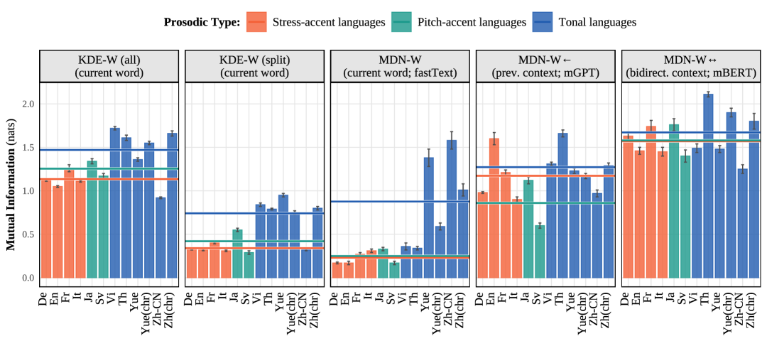
Figure 1: Main Results: Mutual information between pitch and text across languages. Lines show within typological group averages. Error bars show standard deviations from Monte Carlo resampling ($\text{KDE-}{\color[rgb]{0.12890625,0.359375,0.6875}\mathrm{W}}\textsc{(all)}$, $\text{KDE-}{\color[rgb]{0.12890625,0.359375,0.6875}\mathrm{W}}\textsc{(split)}$) or 5-fold cross-validation ($\text{MDN-}{\color[rgb]{0.12890625,0.359375,0.6875}\mathrm{W}}$, $\text{MDN-}{\color[rgb]{0.12890625,0.359375,0.6875}{\color[rgb]{0.12890625,0.359375,0.6875}\mathbf{W}}_{\leftarrow}}$, $\text{MDN-}{\color[rgb]{0.12890625,0.359375,0.6875}{\color[rgb]{0.12890625,0.359375,0.6875}\mathbf{W}}_{\leftrightarrow}}$). We find that tonal languages have higher $\mathrm{MI}$ on average compared to stress-accent and pitch-accent languages.

4 Results

4.1 Main Results

Mutual Information:

The results of our experiment are visualized in Figure˜1, with our different representations of text across the different facets. Horizontal bars show within typological group averages. The data support the typological ordering hypothesis: We observe higher $\mathrm{MI}$ in tonal languages compared to non-tonal languages, for all of our estimation methods. Additionally, we find evidence supporting the tonal >> pitch-accent >> stress-accent hierarchy, especially for our $\text{KDE-}{\color[rgb]{0.12890625,0.359375,0.6875}\mathrm{W}}\textsc{(all)}$, $\text{KDE-}{\color[rgb]{0.12890625,0.359375,0.6875}\mathrm{W}}\textsc{(split)}$, and $\text{MDN-}{\color[rgb]{0.12890625,0.359375,0.6875}\mathrm{W}}$ methods. The ordering is not present for $\text{MDN-}{\color[rgb]{0.12890625,0.359375,0.6875}{\color[rgb]{0.12890625,0.359375,0.6875}\mathbf{W}}_{\leftarrow}}$, where stress-accent languages have higher average $\mathrm{MI}$ than pitch-accent languages, or for $\text{MDN-}{\color[rgb]{0.12890625,0.359375,0.6875}{\color[rgb]{0.12890625,0.359375,0.6875}\mathbf{W}}_{\leftrightarrow}}$, where stress- and pitch-accent languages have almost identical $\mathrm{MI}$. To verify the visual trend in the results, we conducted a Jonckheere trend test (Jonckheere, 1954). This is a non-parametric method that tests whether samples are drawn from different populations with an a priori ordering, compared to a null hypothesis where samples are all drawn from the same population. We use the implementation provided by the clinfun package in R, and approximate our $p$-values using $10,000$ permutations. Our test is significant for $\text{KDE-}{\color[rgb]{0.12890625,0.359375,0.6875}\mathrm{W}}\textsc{(all)}$ ($p<0.05$), $\text{KDE-}{\color[rgb]{0.12890625,0.359375,0.6875}\mathrm{W}}\textsc{(split)}$ ($p<0.05$), and $\text{MDN-}{\color[rgb]{0.12890625,0.359375,0.6875}\mathrm{W}}$ ($p<0.01$) methods, but not for $\text{MDN-}{\color[rgb]{0.12890625,0.359375,0.6875}{\color[rgb]{0.12890625,0.359375,0.6875}\mathbf{W}}_{\leftarrow}}$ or $\text{MDN-}{\color[rgb]{0.12890625,0.359375,0.6875}{\color[rgb]{0.12890625,0.359375,0.6875}\mathbf{W}}_{\leftrightarrow}}$, confirming the visual trend.

Following the logic outline in Section˜3.2, we observe the greatest separation between tonal and non-tonal languages when using estimation techniques that do not take context into account (i.e., $\text{MDN-}{\color[rgb]{0.12890625,0.359375,0.6875}\mathrm{W}}$ and our two KDE-based methods). While estimation methods that incorporate longer context tend to have higher mutual information on average, these methods collapse the difference between typological groups. For example, using $\text{MDN-}{\color[rgb]{0.12890625,0.359375,0.6875}{\color[rgb]{0.12890625,0.359375,0.6875}\mathbf{W}}_{\leftrightarrow}}$, we find the highest average $\mathrm{MI}$ of any model, but we also find almost no difference between tonal and stress-accent languages, in terms of group averages. We suspect this is because $\text{MDN-}{\color[rgb]{0.12890625,0.359375,0.6875}{\color[rgb]{0.12890625,0.359375,0.6875}\mathbf{W}}_{\leftrightarrow}}$, using BERT’s bidirectional context, is capable of representing non-lexical information that can be useful for predicting pitch even in non-tonal languages, e.g., whether a given sentence is a question.

Interestingly, even though prosodic type behavior is consistent across models (i.e., tonal languages always have the highest $\mathrm{MI}$), within each prosodic type, models show variability. For example, our KDE-based methods both suggest that French is the stress-accent language with the highest $\mathrm{MI}$ between pitch and lexical item. However, when using $\text{MDN-}{\color[rgb]{0.12890625,0.359375,0.6875}\mathrm{W}}$, we find the highest $\mathrm{MI}$ for Italian and for $\text{MDN-}{\color[rgb]{0.12890625,0.359375,0.6875}{\color[rgb]{0.12890625,0.359375,0.6875}\mathbf{W}}_{\leftarrow}}$, English. One possibility is that the different ways we represent context between these models lead to different amounts of $\mathrm{MI}$. We return to this point in the larger context of our gradient vs. categorical hypotheses in the discussion.

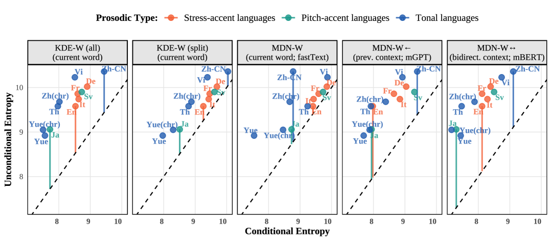
Figure 2: Main Results Separated into Conditional/Unconditional Entropy: Dashed line shows the $y=x$ line. Points show individual languages. Colored lines for En, Ja, and Zh visualize the $\mathrm{MI}$ of these languages, which is the points’ vertical distance from the dotted line.

Conditional and Unconditional Entropy:

To zoom in on these data further, Figure˜2 shows the same results broken down into conditional and unconditional entropy. The difference between these two is the $\mathrm{MI}$, shown in Figure˜1 and visualized here as the vertical distance to the $x=y$ line, which is plotted for English, Japanese, and Mandarin. Overall, we observe a relatively narrow range for both unconditional entropy (ranging from $9$–$10.5$ nats) and conditional entropy (ranging from $7$–$10$ nats) across languages. These data support recent studies showing that information-theoretic properties of human language exist within a narrow bandwidth (Bentz et al., 2017; Wilcox et al., 2023; Pimentel et al., 2020)

When looking at entropy instead of mutual information, we observe more consistency at the language level. For all methods, Vietnamese, Chinese, and German have higher entropy (both conditional and unconditional), and Japanese, Cantonese, Thai, and English have lower entropy. The overall amount of entropy present in a language does not follow typological patterns or even the complexity of a language’s tonal system. Cantonese, which is traditionally analyzed as having nine tones, always has lower entropy values than Mandarin, which is typically analyzed as having only four.

4.2 The Role of Phonotactic Complexity and Syllable Structure

One potential worry with the above results is that the prosodic types might co-vary with other features that could impact our $\mathrm{MI}$ estimation, in particular phonotactic complexity and syllable structure. To alleviate concerns about these potential confounds, we conducted the following checks: First, to examine phonotactic complexity, we used the measure proposed in Pimentel et al. (2020). We found that stress-accent languages possess slightly more complexity than pitch-accent languages ($\mu=3.4,\sigma=0.26$ vs. $\mu=3.0,\sigma=0.01$). However, Pimentel et al. did not report results for our tonal languages. As a second source of data, therefore, we used the World Atlas of Language Structures (WALS; Dryer and Haspelmath, 2013) features of “consonant inventory size” and “vowel inventory size” as a proxy for phonotactic complexity. We find that all of our languages for which data is recorded have “average” consonant inventory sizes, except for Japanese, which is “moderately small.” In addition, all of our languages have “large” vowel inventories, except for Japanese and Mandarin, which are “average.” We take this to mean there are not large differences in these complexity measures by prosodic type.

Turning to syllable structure, using the WALS “syllable structure” feature we find that all of our stress-accent languages have “complex” syllables; and all of our pitch-accent and tone languages have “moderately complex” syllables. Given that we observe the biggest differences in $\mathrm{MI}$ between pitch-accent and tone languages, and only minimal differences between pitch- and stress-accent languages, we do not think that syllable complexity is therefore responsible for differences in $\mathrm{MI}$.

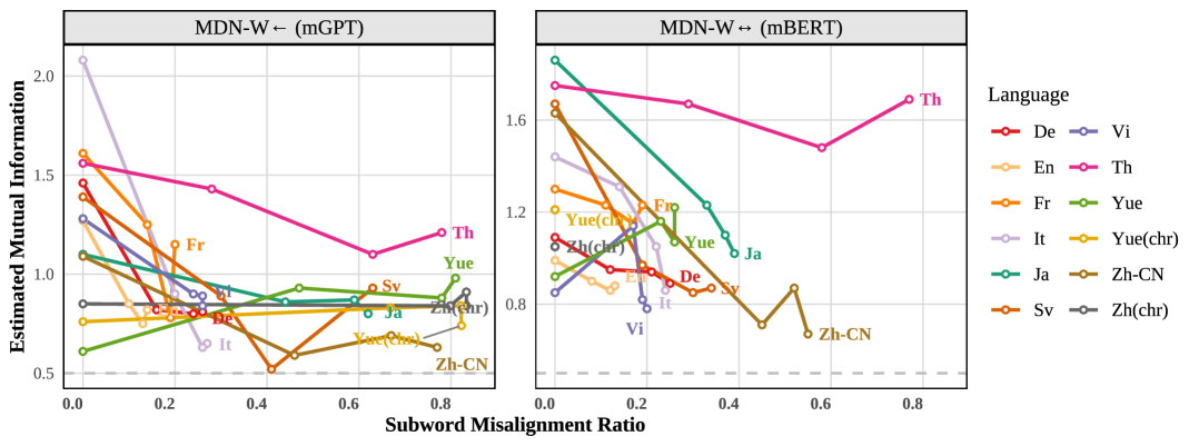
Figure 3: Impact of tokenization on $\mathrm{MI}$ estimation: $x$-axis shows the proportion of words in our dataset tokenized into more than one token. Subsampling data to include only words with one token changes the estimated $\mathrm{MI}$.

4.3 Effect of Subword Tokenization

One difference between $\text{KDE-}{\color[rgb]{0.12890625,0.359375,0.6875}\mathrm{W}}\textsc{(all)}$, $\text{KDE-}{\color[rgb]{0.12890625,0.359375,0.6875}\mathrm{W}}\textsc{(split)}$, and $\text{MDN-}{\color[rgb]{0.12890625,0.359375,0.6875}\mathrm{W}}$, on one hand, and $\text{MDN-}{\color[rgb]{0.12890625,0.359375,0.6875}{\color[rgb]{0.12890625,0.359375,0.6875}\mathbf{W}}_{\leftarrow}}$ and $\text{MDN-}{\color[rgb]{0.12890625,0.359375,0.6875}{\color[rgb]{0.12890625,0.359375,0.6875}\mathbf{W}}_{\leftrightarrow}}$, on the other hand, is that the LLMs that form the basis of the latter two methods (mBERT, mGPT) use subword tokenization schemes. For words that have multiple tokens, we used the embedding of the last token in the word during estimation. It’s possible that this skews or biases our results. Additionally, the number of single-token words varies across languages within our multilingual models, with English having more single-token words than the other languages. To investigate tokenization’s impact, we took each of our initial datasets and subsetted them to include only words with $k$ or fewer tokens. We then re-ran our $\mathrm{MI}$ estimation procedure using only the $\text{MDN-}{\color[rgb]{0.12890625,0.359375,0.6875}{\color[rgb]{0.12890625,0.359375,0.6875}\mathbf{W}}_{\leftarrow}}$ and $\text{MDN-}{\color[rgb]{0.12890625,0.359375,0.6875}{\color[rgb]{0.12890625,0.359375,0.6875}\mathbf{W}}_{\leftrightarrow}}$ methods. This resulted in datasets that were balanced in terms of tokens-per-word, but not in terms of total dataset size.

The results are visualized in Figure˜3. We see that as the percentage of multi-token words decreases, the $\mathrm{MI}$ estimation changes, suggesting that, indeed, this impacts our results. However, the overall picture of the results remains the same—there is no clear separation between tonal, pitch-accent, and stress-accent languages using these models. Interestingly, as the tokens-per-word ratio decreases, the $\mathrm{MI}$ increases for most (although not all) languages, suggesting that the $\mathrm{MI}$ estimates in Figure˜1 are slight underestimates. For additional presentation of these data see Appendix˜A.

5 Discussion

Our experiments supported the typological ordering hypothesis, namely that tonal languages have higher $\mathrm{MI}$ between pitch and text, followed by pitch-accent and stress-accent languages. The ordering of languages according to this prediction is relatively clean, especially for the tonal vs. non-tonal distinction. Among the KDE-based estimates, where we expect the separation to be the strongest, we found only one tonal language (Cantonese, word level) with a lower $\mathrm{MI}$ than any stress-accent language. And with $\text{MDN-}{\color[rgb]{0.12890625,0.359375,0.6875}\mathrm{W}}$, we found that all tonal languages had higher $\mathrm{MI}$ than all stress-accent. Finally, we generally found that pitch-accent languages fell between tonal and stress-accent languages, as expected.

What do our results say about the status of categorical vs. gradient typological theories? On one hand, they could be construed to support the categorical prediction. Using our $\text{MDN-}{\color[rgb]{0.12890625,0.359375,0.6875}\mathrm{W}}$ method, we find a single amount of mutual information ($0.34$ nats) that separates all tonal from non-tonal languages. At the same time, our results demonstrate interesting gradient differences both between and within prosodic types. Firstly, it’s not the case that languages are clearly separated into different modes based on typological type. For example, using our $\text{MDN-}{\color[rgb]{0.12890625,0.359375,0.6875}\mathrm{W}}$ method, there is far more variation in $\mathrm{MI}$ within tonal languages (ranging from $0.36$–$1.58$ nats) than between tonal vs. stress-accent groups ($0.23$ vs. $0.88$ nats). Based on these considerations, we conclude that our data are more closely aligned with the gradient prediction, outlined in Section˜2.1.

We close our theoretical discussion by clarifying the relationship between our definition of a ${\color[rgb]{0.10546875,0.6015625,0.546875}\boldsymbol{\mathrm{p}}}$-language and Greenberg’s (2005) notion of an implicational universal. While implicational universals result in mutual information between linguistic properties, it is not possible to reduce such universals to $\mathrm{MI}$ alone. To take one example, a well-studied implicational universal holds that VSO languages always have prepositions (as opposed to postpositions). This implies that there is mutual information between a language’s word order and its adposition placement. However, if the implication was reversed—VSO implies postpositions—the amount of $\mathrm{MI}$ would remain unchanged. Importantly, implicational universals specify how features of a language covary, not just that they do covary. Zooming out, we can say that implicational universals and ${\color[rgb]{0.10546875,0.6015625,0.546875}\boldsymbol{\mathrm{p}}}$-languages are a larger class of linguistic variation that implies $\mathrm{MI}$ between linguistic features. Further characterizing how mutual information relates to known typological features is an important direction for future research.

Finally, a methodological point: This paper has focused on pitch; however, prosodic typologies operate across a broad range of dimensions. We want to stress that our methods are not only suitable for studying pitch: We initially framed our technical presentation in terms of abstract prosodic categories $\boldsymbol{\mathrm{p}}$. While $\boldsymbol{\mathrm{p}}$ could in theory be all of prosody, it can also be just a single prosodic feature. One could equally well use our methods to examine length-based lexical distinctions, for example, in languages like Turkish. We hope others will build on the technical contributions offered here to study a broader range of prosodic phenomena.

Limitations

One limitation of this work has to do with our dataset: First, the dataset is relatively small, with just $5,000$ sentences per language. Second, we did not control for the number of unique speakers in the dataset, meaning that some languages are overly represented by a single or handful of individuals. For example, our Thai data includes samples from $1,749$ speakers, whereas our Vietnamese data includes samples from just $130$ speakers. One other shortcoming of our dataset is that while our pitch-accent and tonal languages include data from multiple language families, our stress-accent data comes entirely from Indo-European languages. Finally, our dataset did not control for content, meaning the distribution of concepts and, therefore, words could vary substantially across languages. While collecting high-quality audio-text-aligned data across multiple languages is a difficult undertaking, assembling such a dataset and running similar analyses would be an excellent way to further validate the conclusions of this study.

Ethics Statement

We foresee no obvious ethical problems with this research. Furthermore, we do not foresee any obvious risks with this research.

Appendix A Subword Tokenization Follow-up Analysis

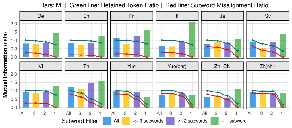
(a) $\text{MDN-}{\color[rgb]{0.12890625,0.359375,0.6875}{\color[rgb]{0.12890625,0.359375,0.6875}\mathbf{W}}_{\leftarrow}}$ (mGPT)

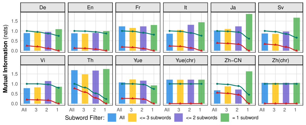
(b) $\text{MDN-}{\color[rgb]{0.12890625,0.359375,0.6875}{\color[rgb]{0.12890625,0.359375,0.6875}\mathbf{W}}_{\leftrightarrow}}$ (mBERT)

Figure 4: Fine-Grained Analysis of Subword Tokenization Effects on $\mathrm{MI}$ Estimation: The x-axis represents subword filtering levels: “All” (no filtering), “3” (subsetted words with at most 3 subword tokens), “2” (at most 2 tokens), and “1” (only single-token words). Bars show estimated $\mathrm{MI}$, the green line represents the retained token ratio after subsetting, and the red line represents the misalignment ratio in the retained data.

In this appendix, we present more fine-grained data concerning the impact of subword tokenization on our $\mathrm{MI}$ estimation. These data are presented in Figure˜4. We find that, in general, filtering out multi-token words increases $\mathrm{MI}$, implying that subword tokenization misalignment adds noise to the estimation procedure. In particular, $\mathrm{MI}$ tends to be highest for our subsampled datasets that include words with only one token—the green bars to the left of each facet. Cantonese (Yue) is an exception, for both of our models, likely due to its many single-character words.

Retained tokens (green line) and misalignment (red line) decrease as we subsample data. However, some languages like English, French, and German retain more data, while Chinese, Thai, and Swedish lose more, resulting in cleaner but smaller datasets for $\mathrm{MI}$ estimation.

Languages also vary in initial misalignment (red lines). English has the lowest initial misalignment, while Chinese and Thai have more, leading to larger $\mathrm{MI}$ gains after filtering and suggesting that $\mathrm{MI}$ is likely underestimated in our main results for these languages when using our $\text{MDN-}{\color[rgb]{0.12890625,0.359375,0.6875}{\color[rgb]{0.12890625,0.359375,0.6875}\mathbf{W}}_{\leftarrow}}$ and $\text{MDN-}{\color[rgb]{0.12890625,0.359375,0.6875}{\color[rgb]{0.12890625,0.359375,0.6875}\mathbf{W}}_{\leftrightarrow}}$ techniques.

Appendix B Hyperparameter and Hyperparameter search

We performed a hyperparameter search using 5-fold cross-validation to tune the $\text{MDN-}{\color[rgb]{0.12890625,0.359375,0.6875}\mathrm{W}}$ model. The search space included:

• Learning rate: 0.01, 0.001

• Dropout: 0.2, 0.5

• Hidden layers: 15, 20, 30

• Hidden units: 512, 1024

Models were trained for a maximum of 50 epochs using the AdamW optimizer with weight decay (L2 regularization = $0.001$) and early stopping (patience = 3) based on validation loss. The best hyperparameters were selected based on average performance across the 5 folds and evaluated on the test set.

For our $\text{MDN-}{\color[rgb]{0.12890625,0.359375,0.6875}{\color[rgb]{0.12890625,0.359375,0.6875}\mathbf{W}}_{\leftarrow}}$, using mGPT (ai-forever/mGPT) and $\text{MDN-}{\color[rgb]{0.12890625,0.359375,0.6875}{\color[rgb]{0.12890625,0.359375,0.6875}\mathbf{W}}_{\leftrightarrow}}$ using mBERT (bert-base-multilingual-cased) models, we fine-tuned using AdamW (weight decay = 0.1), a learning rate of $5.0\times 10^{-5}$ with ReduceLROnPlateau (factor = 0.1, patience = 2), batch size 16 (effective 64), gradient clipping at 1.0, dropout of 0.1 (applied to the MLP head), and early stopping (patience = 3). For $\text{MDN-}{\color[rgb]{0.12890625,0.359375,0.6875}{\color[rgb]{0.12890625,0.359375,0.6875}\mathbf{W}}_{\leftarrow}}$ using mGPT, we fine-tune only the last eight transformer layers, freezing the rest for efficiency, resulting in 612M trainable parameters (out of 1.4B total). For $\text{MDN-}{\color[rgb]{0.12890625,0.359375,0.6875}{\color[rgb]{0.12890625,0.359375,0.6875}\mathbf{W}}_{\leftrightarrow}}$ using mBERT, all layers are fine-tuned, for 177M trainable parameters.

References

- Ardila et al. (2020) Rosana Ardila, Megan Branson, Kelly Davis, Michael Kohler, Josh Meyer, Michael Henretty, Reuben Morais, Lindsay Saunders, Francis Tyers, and Gregor Weber. 2020. Common voice: A massively-multilingual speech corpus. In Proceedings of the Twelfth Language Resources and Evaluation Conference, pages 4218–4222, Marseille, France. European Language Resources Association.
- Baylor et al. (2024) Emi Baylor, Esther Ploeger, and Johannes Bjerva. 2024. Multilingual gradient word-order typology from Universal Dependencies. In Proceedings of the 18th Conference of the European Chapter of the Association for Computational Linguistics (Volume 2: Short Papers), pages 42–49, St. Julian’s, Malta. Association for Computational Linguistics.
- Beirlant et al. (1997) Jan Beirlant, Edward J Dudewicz, László Györfi, Edward C Van der Meulen, et al. 1997. Nonparametric entropy estimation: An overview. International Journal of Mathematical and Statistical Sciences, 6(1):17–39.
- Bentz et al. (2017) Christian Bentz, Dimitrios Alikaniotis, Michael Cysouw, and Ramon Ferrer-i Cancho. 2017. The entropy of words—learnability and expressivity across more than 1000 languages. Entropy, 19(6).
- Bishop (1994) Christopher M Bishop. 1994. Mixture density networks.
- Bojanowski et al. (2017) Piotr Bojanowski, Edouard Grave, Armand Joulin, and Tomas Mikolov. 2017. Enriching word vectors with subword information. Transactions of the Association for Computational Linguistics, 5:135–146.
- Chomsky (1993) Noam Chomsky. 1993. Lectures on government and binding: The Pisa lectures. 9. Walter de Gruyter.
- Croft (2002) William Croft. 2002. Typology and universals. Cambridge University Press.
- Culicover (1997) Peter W Culicover. 1997. Principles and parameters: An introduction to syntactic theory. Oxford University Press.
- Dautriche et al. (2017) Isabelle Dautriche, Kyle Mahowald, Edward Gibson, and Steven T. Piantadosi. 2017. Wordform similarity increases with semantic similarity: An analysis of 100 languages. Cognitive Science, 41(8):2149–2169.
- Devlin et al. (2019) Jacob Devlin, Ming-Wei Chang, Kenton Lee, and Kristina Toutanova. 2019. BERT: Pre-training of deep bidirectional transformers for language understanding. In Proceedings of the 2019 Conference of the North American Chapter of the Association for Computational Linguistics: Human Language Technologies, Volume 1 (Long and Short Papers), pages 4171–4186, Minneapolis, Minnesota. Association for Computational Linguistics.
- Dryer and Haspelmath (2013) Matthew S. Dryer and Martin Haspelmath, editors. 2013. WALS Online (v2020.4). Zenodo.
- Dyer et al. (2021) William Dyer, Richard Futrell, Zoey Liu, and Greg Scontras. 2021. Predicting cross-linguistic adjective order with information gain. In Findings of the Association for Computational Linguistics: ACL-IJCNLP 2021, pages 957–967, Online. Association for Computational Linguistics.
- Ethnologue (2023) Ethnologue. 2023. Ethnologue: Languages of the world.
- Futrell et al. (2020) Richard Futrell, Edward Gibson, and Roger P Levy. 2020. Lossy-context surprisal: An information-theoretic model of memory effects in sentence processing. Cognitive Science, 44(3):e12814.
- Greenberg (2005) Joseph H. Greenberg. 2005. Language Universals: With Special Reference to Feature Hierarchies. De Gruyter Mouton, Berlin, New York.
- Hagège (1992) Claude Hagège. 1992. Morphological typology. International encyclopedia of linguistics, 3:7–8.
- Hyman (2006) Larry M Hyman. 2006. Word-prosodic typology. Phonology, 23(2):225–257.
- Jonckheere (1954) A. R. Jonckheere. 1954. A distribution-free k-sample test against ordered alternatives. Biometrika, 41(1/2):133–145.
- Kemp et al. (2018) Charles Kemp, Yang Xu, and Terry Regier. 2018. Semantic typology and efficient communication. Annual Review of Linguistics, 4:109–128.
- Lesci et al. (2025) Pietro Lesci, Clara Meister, Thomas Hofmann, Andreas Vlachos, and Tiago Pimentel. 2025. Causal estimation of tokenisation bias. In Proceedings of the 63rd Annual Meeting of the Association for Computational Linguistics (Volume 1: Long Papers). Association for Computational Linguistics.
- Levshina et al. (2023) Natalia Levshina, Savithry Namboodiripad, Marc Allassonnière-Tang, Mathew Kramer, Luigi Talamo, Annemarie Verkerk, Sasha Wilmoth, Gabriela Garrido Rodriguez, Timothy Michael Gupton, Evan Kidd, Zoey Liu, Chiara Naccarato, Rachel Nordlinger, Anastasia Panova, and Natalia Stoynova. 2023. Why we need a gradient approach to word order. Linguistics, 61(4):825–883.
- McAuliffe et al. (2017) Michael McAuliffe, Michaela Socolof, Sarah Mihuc, Michael Wagner, and Morgan Sonderegger. 2017. Montreal forced aligner: Trainable text-speech alignment using Kaldi. In Interspeech, volume 2017, pages 498–502.
- Parzen (1962) Emanuel Parzen. 1962. On estimation of a probability density function and mode. The Annals of Mathematical Statistics, 33(3):1065–1076.
- Piantadosi et al. (2011) Steven T Piantadosi, Harry Tily, and Edward Gibson. 2011. Word lengths are optimized for efficient communication. Proceedings of the National Academy of Sciences, 108(9):3526–3529.
- Pimentel et al. (2019) Tiago Pimentel, Arya D. McCarthy, Damian Blasi, Brian Roark, and Ryan Cotterell. 2019. Meaning to form: Measuring systematicity as information. In Proceedings of the 57th Annual Meeting of the Association for Computational Linguistics, pages 1751–1764, Florence, Italy. Association for Computational Linguistics.
- Pimentel et al. (2023) Tiago Pimentel, Clara Meister, Ethan Wilcox, Kyle Mahowald, and Ryan Cotterell. 2023. Revisiting the optimality of word lengths. In Proceedings of the 2023 Conference on Empirical Methods in Natural Language Processing, pages 2240–2255, Singapore. Association for Computational Linguistics.
- Pimentel et al. (2020) Tiago Pimentel, Brian Roark, and Ryan Cotterell. 2020. Phonotactic complexity and its trade-offs. Transactions of the Association for Computational Linguistics, 8:1–18.
- Prince and Smolensky (2004) Alan Prince and Paul Smolensky. 2004. Optimality theory: Constraint interaction in generative grammar. Optimality Theory in Phonology: A reader, pages 1–71.
- Regev et al. (2025) Tamar I Regev, Chiebuka Ohams, Shaylee Xie, Lukas Wolf, Evelina Fedorenko, Alex Warstadt, Ethan G Wilcox, and Tiago Pimentel. 2025. The time scale of redundancy between prosody and linguistic context. In Proceedings of the 63rd Annual Meeting of the Association for Computational Linguistics (Volume 1: Long Papers). Association for Computational Linguistics.
- Saussure (1916) Ferdinand de Saussure. 1916. Course in General Linguistics. Columbia University Press, New York. English edition of June 2011, based on the 1959 translation by Wade Baskin.
- Shannon (1948) Claude Elwood Shannon. 1948. A mathematical theory of communication. The Bell System Technical Journal, 27(3):379–423.
- Sheather (2004) Simon J Sheather. 2004. Density estimation. Statistical Science, pages 588–597.
- Shliazhko et al. (2024) Oleh Shliazhko, Alena Fenogenova, Maria Tikhonova, Anastasia Kozlova, Vladislav Mikhailov, and Tatiana Shavrina. 2024. mGPT: Few-shot learners go multilingual. Transactions of the Association for Computational Linguistics, 12:58–79.
- Silverman (1986) Bernard W Silverman. 1986. Density estimation for statistics and data analysis. Routledge.
- Socolof et al. (2022) Michaela Socolof, Jacob Louis Hoover, Richard Futrell, Alessandro Sordoni, and Timothy J. O’Donnell. 2022. Measuring morphological fusion using partial information decomposition. In Proceedings of the 29th International Conference on Computational Linguistics, pages 44–54, Gyeongju, Republic of Korea. International Committee on Computational Linguistics.
- Steuer et al. (2023) Julius Steuer, Johann-Mattis List, Badr M. Abdullah, and Dietrich Klakow. 2023. Information-theoretic characterization of vowel harmony: A cross-linguistic study on word lists. In Proceedings of the 5th Workshop on Research in Computational Linguistic Typology and Multilingual NLP, pages 96–109, Dubrovnik, Croatia. Association for Computational Linguistics.
- Suni et al. (2017) Antti Suni, Juraj Šimko, Daniel Aalto, and Martti Vainio. 2017. Hierarchical representation and estimation of prosody using continuous wavelet transform. Computer Speech & Language, 45:123–136.
- Tibshirani and Efron (1993) Robert J Tibshirani and Bradley Efron. 1993. An introduction to the bootstrap. Monographs on Statistics and Applied Probability, 57(1):1–436.
- Virtanen et al. (2020) Pauli Virtanen, Ralf Gommers, Travis E Oliphant, Matt Haberland, Tyler Reddy, David Cournapeau, Evgeni Burovski, Pearu Peterson, Warren Weckesser, Jonathan Bright, et al. 2020. SciPy 1.0: Fundamental algorithms for scientific computing in Python. Nature Methods, 17(3):261–272.
- Wilcox et al. (2023) Ethan G Wilcox, Tiago Pimentel, Clara Meister, Ryan Cotterell, and Roger P Levy. 2023. Testing the predictions of surprisal theory in 11 languages. Transactions of the Association for Computational Linguistics, 11:1451–1470.
- Wolf et al. (2023) Lukas Wolf, Tiago Pimentel, Evelina Fedorenko, Ryan Cotterell, Alex Warstadt, Ethan Wilcox, and Tamar Regev. 2023. Quantifying the redundancy between prosody and text. In Proceedings of the 2023 Conference on Empirical Methods in Natural Language Processing, pages 9765–9784, Singapore. Association for Computational Linguistics.
- Yip (2002) Moira Yip. 2002. Tone. Cambridge Textbooks in Linguistics. Cambridge University Press.
- Zaslavsky et al. (2018) Noga Zaslavsky, Charles Kemp, Terry Regier, and Naftali Tishby. 2018. Efficient compression in color naming and its evolution. Proceedings of the National Academy of Sciences, 115(31):7937–7942.
- Zaslavsky et al. (2021) Noga Zaslavsky, Mora Maldonado, and Jennifer Culbertson. 2021. Let’s talk (efficiently) about us: Person systems achieve near-optimal compression. In Proceedings of the Annual Meeting of the Cognitive Science Society, volume 43.
- Zipf (1949) George K. Zipf. 1949. Human Behavior and the Principle of Least Effort. Addison-Wesley Press.