On the choice of optimization norm for Anderson acceleration of the Picard iteration for Navier-Stokes equations

Abstract.

Recently developed convergence theory for Anderson acceleration (AA) assumes that the AA optimization norm matches the norm of the Hilbert space that the fixed point function is defined on. While this seems a natural assumption, it may not be the optimal choice in terms of convergence of the iteration or computational efficiency. For the Picard iteration for the Navier-Stokes equations (NSE), the associated Hilbert space norm is $H^{1}_{0}(\Omega),$ which is inefficient to implement in a large scale HPC setting since it requires multiplication of global coefficient vectors by the stiffness matrix. Motivated by recent numerical tests that show using the $\ell^{2}$ norm produces similar convergence behavior as $H^{1}_{0}$ does, we revisit the convergence theory of [Pollock et al, SINUM 2019] and find that i) it can be improved with a sharper treatment of the nonlinear terms; and ii) in the case that the AA optimization norm is changed to $L^{2}$ (and by extension $\ell^{2}$ or $L^{2}$ using a diagonally lumped mass matrix), a new convergence theory is developed that provides an essentially equivalent estimate as the $H^{1}_{0}$ case. Several numerical tests illustrate the new theory, and the theory and tests reveal that one can interchangeably use the norms $H^{1}_{0}$, $L^{2}$, $\ell^{2}$ or $L^{2}$ with diagonally lumped mass matrix for the AA optimization problem without significantly affecting the overall convergence behavior. Thus, one is justified to use $\ell^{2}$ or diagonally lumped $L^{2}$ for the AA optimization norm in Anderson accelerated Picard iterations for large scale NSE problems.

1. Introduction

We consider an Anderson accelerated nonlinear solver for the Navier-Stokes equations (NSE) that model incompressible fluid flow, which are given for steady flows on a domain $\Omega\subset\mathbb{R}^{d},d=2,3$ by

(1.1) $$\left\{\begin{aligned} -\nu\Delta u+u\cdot\nabla u+\nabla p&={f}\quad\text{in}~\Omega,\\ \nabla\cdot{u}&=0\quad\text{in}~\Omega,\\ {u}&=0\quad\text{on}~~\partial\Omega,\end{aligned}\right.$$

where $u$ and $p$ are the unknown fluid velocity and pressure, $\nu>0$ is the kinematic viscosity, and ${f}$ is a given external forcing (such as gravity or bouyancy). The Reynolds number $Re\sim\frac{1}{\nu}$ is a physical constant that describes the complexity of a flow: higher $Re$ is typically associated with more complex physics and non-unique solutions of (1.1). We consider the system (1.1) equipped with homogenous Dirichlet boundary conditions, but our results can extend to nonhomogeneous mixed Dirichlet/Neumann boundary conditions as well as to solving the time dependent NSE at a fixed time step in a time stepping scheme. It is well known that (1.1) admits weak solutions for any $\nu>0$ and $f\in H^{-1}(\Omega)$, and under a small data condition $\kappa:=M\nu^{-2}\|f\|_{H^{-1}}<1$ (where $M$ is a domain-size dependent constant, see section 2), solutions are unique [10, 31, 16].

A common nonlinear solver for (1.1) is the Picard iteration, which is given by

$$-\nu\Delta u_{k+1}+u_{k}\cdot\nabla u_{k+1}+\nabla p_{k+1} ={f},$$

$$\nabla\cdot{u}_{k+1} =0,$$

$$u_{k+1}|_{\partial\Omega} =0.$$

The Picard iteration for the NSE is globally stable, and is globally linearly convergent with rate $\kappa$ if $\kappa<1$. As $Re$ increases (i.e. $\kappa$ increases), the convergence of Picard slows, and for $Re$ large enough the method fails to converge [23, 22]. Unfortunately, this failure occurs for $Re$ well within the range of physically relevant problems [16]. To improve the speed and robustness of Picard for the NSE, incorporating Anderson acceleration (AA) was proposed in [23] and was found to significantly accelerate a converging Picard iteration as well as dramatically increase the range of $Re$ for which convergence could be achieved. Moreover, it was rigorously proven in [23] that AA improves the linear convergence rate of Picard by scaling it by the gain of the AA optimization problem (details in section 2), giving theory to the improvements seen in computational tests. We note that AA-Picard was also shown to be a good nonlinear preconditioner for the Newton iteration for the NSE in [22, 18], and also that several followup studies to [23] found analytically and numerically that AA was effective at accelerating and enabling convergence of several other related Picard-type iterations for other PDEs e.g. [17, 24, 9]. In fact, AA has been found effective at improving convergence for many other nonlinear solvers, see [21, 15, 26] and references therein, and we note more AA background is given in Section 2.

The purpose of this paper is to further investigate AA-Picard for the NSE, and in particular to consider choices of AA optimization norms that are more efficient than $H^{1}_{0}$ to determine if they provide the same benefits to solver convergence. The theory from [23] uses the $H^{1}_{0}$ norm, which appears to follow naturally in the analysis. However, recent numerical tests in [13, 20] show that if the $\ell^{2}$ norm is used in the optimization, convergence results are essentially the same as when $H^{1}_{0}$ is used. This is critically important because optimization in $\ell^{2}$ is much more computationally efficient than $H^{1}_{0}$ in HPC, i.e. across many processors such as when using deal.ii [1] on a supercomputer, since $H^{1}_{0}$ requires multiplication of the global residual vectors by the stiffness matrix, which is a slow operation in that setting [13]. However, one should probably not change the AA optimization norm in an ad-hoc manner without mathematical justification (especially if one is a mathematician) and expect convergence behavior to remain unchanged: recent work on second order nonlinear elliptic problems showed that the choice of AA optimization norm matters in terms of residual convergence, and the choice of this norm can significantly affect (i.e. enable or prevent) convergence [36].

We prove in Section 3 that when $H^{1}_{0}$ is used as the AA optimization norm, a sharper convergence result than proven in [23] is established through sharper estimates of the nonlinear terms. Interestingly, and surprisingly, this estimate shows that the improvement in convergence relies on both the gain factor of the AA optimization in the $H^{1}_{0}$ norm as well as gain factor for the $L^{2}$ norm, even though the $L^{2}$ norm is never used in the algorithm for this case. We then extend this sharpened analysis to the case when $L^{2}$ is used as the AA optimization norm, and find an equivalent result where the gain factor again depends on both the $L^{2}$ and $H^{1}_{0}$ optimization problem gain factors. This is perfectly consistent what numerical tests in [13, 20] found, which is that very similar convergence behavior will be found whether the $L^{2}$ or $H^{1}_{0}$ norm is used for the AA optimization.

Since using either the $\ell^{2}$ norm or the $L^{2}$ norm approximated by using a diagonally lumped mass matrix (hereafter called ‘diagonally lumped $L^{2}$ norm’) norms give very close approximations to using the $L^{2}$ norm for the AA optimization, our analysis also implies these norms are also excellent choices since they give essentially the same convergence behavior as $L^{2}$ and thus also $H^{1}_{0}$, but are much more computationally efficient for large scale problems. In fact, in all of our tests, convergence results from using $L^{2}$ and diagonally lumped $L^{2}$ norms are visually indistinguishable until the $H^{1}$ residual drops below $10^{-5}$. Section 4 shows results of several numerical tests that illustrate the theory and show that one can confidently use either $\ell^{2}$ or diagonally lumped $L^{2}$ as the AA optimization norm in the HPC setting and get both optimal convergence and computational efficiency.

This paper is arranged as follows. Section 2 defines notation, gives mathematical preliminaries, and provides background on Navier-Stokes equations, the Picard iteration, Anderson acceleration, and AA-Picard. Our new analysis is given in section 3, and numerical tests are found in section 4. Finally, conclusions and future directions are discussed in section 5.

2. Notation and Preliminaries

We consider an open connected set $\Omega\subset\mathbb{R}^{d}$ (d=2 or 3) as the domain, and the $L^{2}(\Omega)$ inner product and norm are denoted as $(\cdot,\cdot)$ and $\|\cdot\|$, respectively. Other norms will be clearly labeled with subscripts. The notation $\langle\cdot,\cdot\rangle$ is used to represent the duality pairing between $H^{-1}$ and $X$. We use $\|\cdot\|_{-1}$ to denote the norm on $H^{-1}(\Omega)$.

Define the natural pressure and velocity function spaces for the NSE by

$$Q:=\{q\in{L}^{2}(\Omega):\int_{\Omega}q\ dx=0\},$$

$$X:=\{v\in H^{1}\left(\Omega\right):v=0~~\text{on}~\partial\Omega\},$$

along with the divergence-free velocity space

$$V:=\{v\in X:(\nabla\cdot v,q)=0\ \forall q\in Q\}.$$

The Poincaré inequality holds on $X$: there exists a constant $C_{P}(\Omega)$ depending only on the domain size which satisfies

(2.1) $$\|\phi\|\leq C_{P}\|\nabla\phi\|\mbox{ for all }\phi\in X.$$

We use the skew-symmetric form of the nonlinear term: for all $v,w,z\in X,$

$$b^{*}(v,w,z)=(v\cdot\nabla w,z)+\frac{1}{2}((\nabla\cdot v)w,z).$$

One could also use other energy preserving formulations such as rotational and EMAC forms [5] and get the same results as we find herein.

A key property of $b^{*}$ is that

$$b^{*}(v,w,w)=0\ \forall w,v\in X.$$

If the first argument of $b^{*}$ is divergence-free, i.e. it satisfies $\|\nabla\cdot v\|=0$, then skew-symmetry has no effect. However, when using certain finite element subspaces of $X$ and $Q$ (such as Taylor-Hood elements), the discretely divergence-free space does not contain only divergence-free functions. Hence, to be general, we utilize skew-symmetry in our analysis.

2.1. Finite element preliminaries

Let $\tau_{h}(\Omega)$ be a conforming mesh and $X_{h}(\tau_{h})\times Q_{h}(\tau_{h})\subset X\times Q$ be conforming finite element spaces for the velocity and pressure, respectively. We require the pair $(X_{h},Q_{h})$ to satisfy the inf-sup condition

$$\sup_{0\neq v\in X_{h}}\frac{(\nabla\cdot v,q)}{\|\nabla v\|}\geq\beta\|q\|\qquad\forall q\in Q_{h},$$

for some $\beta>0$ that is independent of $h$. Commonly used examples are the Taylor-Hood and Scott-Vogelius elements, with the latter possibly requiring meshes to have a particular macro-element structure depending on the polynomial degree [14, 11, 3, 37].

Define the discretely divergence-free space by

$$V_{h}:=\{v\in X_{h}:(\nabla\cdot v,q)=0\ \forall q\in Q_{h}\}.$$

Denote the discrete Stokes operator by $\Delta_{h}$, which satisfies: Given $\phi\in H^{1}(\Omega)$, $\Delta_{h}\phi\in V_{h}$ satisfies

$$(\Delta_{h}\phi,v)=(\nabla\phi,\nabla v)\ \ \forall v\in V_{h}.$$

Thanks to [12], we know for $\phi\in V_{h}$ that

(2.2) $$\|\nabla\phi\|_{L^{3}}+\|\phi\|_{L^{\infty}}\leq C\|\nabla\phi\|^{1/2}\|\Delta_{h}\phi\|^{1/2}.$$

2.2. Bounding $b^{*}$ preliminaries

Bounding the $b^{*}$ functional is critical to our residual convergence analysis. There are several ways to get bounds, as is stated in the following lemma.

Lemma 2.1.

Suppose $v,w,z\in X$. Then there exists $M=M(\Omega)$ such that

(2.3) $$|b^{*}(v,w,z)| \leq MC_{P}^{-1/2}\|v\|^{1/2}\|\nabla v\|^{1/2}\|\nabla w\|\|\nabla z\|,$$

(2.4) $$|b^{*}(v,w,z)| \leq M\|\nabla v\|\|\nabla w\|\|\nabla z\|,$$

(2.5) $$|b^{*}(v,w,z)| \leq\frac{1}{2}\|v\cdot\nabla\chi+\nabla\cdot(v\chi)\|_{-1}\|\nabla z\|.$$

Further, if additionally $w\in V_{h}$, then there exists $c=c(\Omega)$ such that

(2.6) $$|b^{*}(v,w,z)|\leq c\|v\|\|\nabla w\|^{1/2}\|\Delta_{h}w\|^{1/2}\|\nabla z\|.$$

Proof.

We start with Green’s theorem to obtain

$$b^{*}(v,w,z)=\frac{1}{2}(v\cdot\nabla w,z)-\frac{1}{2}(v\cdot\nabla z,w).$$

Next, using Hölder’s inequality, we get that

$$b^{*}(v,w,z) =\frac{1}{2}(v\cdot\nabla w,z)-\frac{1}{2}(v\cdot\nabla z,w)$$

$$\leq\frac{1}{2}\|v\|_{L^{p}}\|\nabla w\|_{L^{q}}\|z\|_{L^{r}}+\frac{1}{2}\|v\|_{L^{p^{\prime}}}\|\nabla z\|_{L^{q^{\prime}}}\|w\|_{L^{r^{\prime}}},$$

with $\frac{1}{p}+\frac{1}{q}+\frac{1}{r}=\frac{1}{p^{\prime}}+\frac{1}{q^{\prime}}+\frac{1}{r^{\prime}}=1$. Choosing $r=r^{\prime}=6$, $q=q^{\prime}=2$ and $p=p^{\prime}=3$ followed by a Sobolev inequality from the embedding of $H^{1}(\Omega)$ into $L^{6}(\Omega)$ produces

(2.7) $$b^{*}(v,w,z)\leq C_{6}\|v\|_{L^{3}}\|\nabla w\|\|\nabla z\|.$$

Next, we apply to (2.7) the bound on $L^{3}(\Omega)$ from Gagliardo-Nirenberg $\|\phi\|_{L^{3}}\leq C_{3}\|\phi\|^{1/2}\|\nabla\phi\|^{1/2}$ and obtain

(2.8) $$b^{*}(v,w,z)\leq C_{6}C_{3}\|v\|^{1/2}\|\nabla v\|^{1/2}\|\nabla w\|\|\nabla z\|.$$

An application of Poincarè to $\|v\|$ will produce the bound (2.4), with $M=C_{P}^{1/2}C_{6}C_{3}$. Using this definition of $M$ in (2.8), we establish (2.3) as well.

For the third bound, we use Hölder with $L^{2}$-$L^{3}$-$L^{6}$ and $L^{2}$-$L^{2}$-$L^{\infty}$, respectively, to get

$$b^{*}(v,w,z)\leq\frac{1}{2}\|v\|\|\nabla w\|_{L^{3}}\|z\|_{L^{6}}+\frac{1}{2}\|v\|\|\nabla z\|\|w\|_{L^{\infty}}.$$

Using Sobolev inequalities and (2.2), we obtain the bound (2.6),

$$b^{*}(v,w,z)\leq c\|v\|\|\nabla w\|^{1/2}\|\Delta_{h}w\|^{1/2}\|\nabla z\|.$$

For the last bound, starting after the application of Green’s theorem above, we apply Green one more time on the second right hand side term to get

$$b^{*}(v,w,z)=\frac{1}{2}(v\cdot\nabla w,z)+\frac{1}{2}(\nabla\cdot(vw),z)=\frac{1}{2}(v\cdot\nabla w+\nabla\cdot(vw),z).$$

Now multiply and divide by $\|\nabla z\|$ and use the definition of the $H^{-1}$ norm to reveal the final bound of the lemma,

(2.9) $$b^{*}(v,\chi,z)=\frac{\frac{1}{2}(v\cdot\nabla\chi+\nabla\cdot(v\chi),z)}{\|\nabla z\|}\|\nabla z\|\leq\frac{1}{2}\|v\cdot\nabla\chi+\nabla\cdot(v\chi)\|_{-1}\|\nabla z\|.$$

∎

2.3. NSE preliminaries

The weak form of the NSE (1.1) is given by [16]: Find $u\in V$ satisfying

(2.10) $$\nu(\nabla u,\nabla v)+b^{*}(u,u,v)=\langle f,v\rangle\ \forall v\in V.$$

Solutions exist for the weak steady NSE system (2.10) for any $f\in H^{-1}(\Omega)$ and $\nu>0$ [10, 16], and any such solution satisfies

(2.11) $$\|\nabla u\|\leq\nu^{-1}\|f\|_{-1}.$$

A sufficient condition for uniqueness of solutions is that the data satisfy the smallness condition $\kappa:=M\nu^{-2}\|f\|_{-1}<1$ [10, 16]. While $\kappa<1$ is not necessary for uniqueness, it is known that for sufficiently large data (i.e. $\kappa$ large enough), uniqueness breaks down and the NSE will admit multiple solutions [16].

The finite element NSE formulation is given by: Find $u\in V_{h}$ satisfying

(2.12) $$\nu(\nabla u,\nabla v)+b^{*}(u,u,v)=\langle f,v\rangle\ \forall v\in V_{h}.$$

The same results as above for boundedness and well-posedness that hold in the $V$-formulation will also hold in the $V_{h}$ formulation (with essentially identical proofs), despite $V_{h}$ not necessarily being a subset of $V$.

2.4. Picard for NSE preliminaries

The finite element form of the Picard iteration for the NSE is: Given $u_{k}\in V_{h}$, find $u_{k+1}\in V_{h}$ satisfying

(2.13) $$\nu(\nabla u_{k+1},\nabla v)+b^{*}(u_{k},u_{k+1},v)=\langle f,v\rangle\ \forall v\in V_{h}.$$

It is shown in [23] that the solution operator $g:V_{h}\rightarrow V_{h}$ associated with (2.13) is well-defined and uniformly bounded as

(2.14) $$\|\nabla g(u_{k})\|=\|\nabla u_{k+1}\|\leq\nu^{-1}\|f\|_{-1}.$$

Thus we can write (2.13) as a fixed point iteration $u_{k+1}=g(u_{k})$.

It is also known that the error in Picard (i.e. the difference to (2.12)) satisfies [10, 23]

(2.15) $$\|\nabla(u-u_{k+1})\|\leq\kappa\|\nabla(u-u_{k})\|,$$

and the residual satisfies

(2.16) $$\|\nabla(u_{k+1}-u_{k})\|\leq\kappa\|\nabla(u_{k}-u_{k-1})\|.$$

Hence if $\kappa<1$, it is expected that the Picard iteration will convergence linearly with rate $\kappa$ to the unique weak NSE solution

The solution to (2.13) is also bounded in a higher order norm. Taking $v=\Delta_{h}u_{k+1}$, we observe that

$$\nu\|\Delta_{h}u_{k+1}\|^{2}=(f,\Delta_{h}u_{k+1})-b^{*}(u_{k},u_{k+1},\Delta_{h}u_{k+1}),$$

and after applying Cauchy-Schwarz on the first right hand side term and Hölder on the second we get

$$\nu\|\Delta_{h}u_{k+1}\|^{2}\leq\|f\|\|\Delta_{h}u_{k+1}\|+\|u_{k}\|_{L^{6}}\|\nabla u_{k+1}\|_{L^{3}}\|\Delta_{h}u_{k+1}\|+\frac{1}{2}\|\nabla\cdot u_{k}\|\|u_{k+1}\|_{L^{\infty}}\|\Delta_{h}u_{k+1}\|.$$

Applying (2.2) and reducing now provides

$$\nu\|\Delta_{h}u_{k+1}\| \leq\|f\|+C_{s}\|\nabla u_{k}\|\|\nabla u_{k+1}\|^{1/2}\|\Delta_{h}u_{k+1}\|^{1/2}$$

$$\leq\|f\|+C_{s}\nu^{-3/2}\|f\|_{-1}^{3/2}\|\Delta_{h}u_{k+1}\|^{1/2}$$

$$\leq\|f\|+\frac{\nu^{-1}}{2}(C_{s}\nu^{-3/2}\|f\|_{-1}^{3/2})^{2}+\frac{\nu}{2}\|\Delta_{h}u_{k+1}\|,$$

with the last step thanks to Young’s inequality. Reducing again yields

(2.17) $$\|\Delta_{h}u_{k+1}\|\leq\nu^{-1}\|f\|+C\nu^{-4}\|f\|_{-1}^{3}.$$

2.5. Anderson acceleration preliminaries

AA is defined as follows, for a given fixed point function $G:H\rightarrow H$ for a Hilbert space $H$ and optimization in a norm denoted $\|\cdot\|_{*}$ (for our case of interest, $G=g$ from above, $X=H^{1}_{0}(\Omega)$, and we will consider varying choices of optimization norms).

Algorithm 2.2 (Anderson acceleration [2]).

Anderson acceleration with depth $m$ reads:
Step 0: Choose $u_{0}\in X.$
Step 1: Find $\tilde{u}_{1}\in X$ such that $\tilde{u}_{1}=G(u_{0})$. Set $u_{1}=\tilde{u}_{1}$.
Step $k$: For $k+1=1,2,3,\ldots$ Set $m_{k}=\min\{k,m\}.$
[a.] Find $\tilde{u}_{k+1}=G(u_{k})$.
[b.] Solve the minimization problem for $\{\alpha_{j}^{k+1}\}_{k-m_{k}}^{k}$

$$\min_{\sum\limits_{j=k-m_{k}}^{k}\alpha_{j}^{k+1}=1}\left\|\sum\limits_{j=k-m_{k}}^{k}\alpha_{j}^{k+1}(\tilde{u}_{j+1}-u_{j})\right\|_{*}.$$

[c.] Set

$$u_{k+1}=\beta_{k+1}\sum\limits_{j=k-m_{k}}^{k}\alpha_{j}^{k+1}\tilde{u}_{j+1}+(1-\beta_{k+1})\sum\limits_{j=k-m_{k}}^{k}\alpha_{j}^{k+1}u_{j},$$

for damping parameter $0<\beta_{k}\leq 1$.

We note that $H$ need not be a Hilbert space to apply the AA algorithm. However, convergence analyses of AA do require this [23, 19]. That is, one can use a non-Hilbert space norm, but it is not clear if or how AA will improve convergence and the AA convergence theory of [19, 23, 7] falls no longer holds.

Provided $H$ is a Hilbert space, an implementation of AA is given as follows [21]. Define $F$ to be the rectangular matrix with columns $\{\tilde{u}_{j+1}-u_{j}\}_{j=k-m_{k}}^{k}$, and the vector $\alpha=\{\alpha_{j}\}_{j=k-m_{k}}^{k}$. Then the optimization problem can be written equivalently as

$$\min_{\sum\limits_{j=k-m}^{k}\alpha_{j}^{k+1}=1}\left\|\sum\limits_{j=k-m}^{k}\alpha_{j}^{k+1}(\tilde{u}_{j+1}-u_{j})\right\|_{*}\iff\min_{\sum\limits_{j=k-m}^{k}\alpha_{j}^{k+1}=1}\left\|F\alpha\right\|_{*}^{2}$$

In the finite element setting, $\|F\alpha\|_{X}^{2}=\alpha^{T}F^{T}MF\alpha$, where for example $M$ is the mass matrix if $*=L^{2}(\Omega)$, the stiffness matrix if $*=H^{1}_{0}(\Omega)$, or the identity matrix if $*=\ell^{2}$.

Next, define the reduced $QR=M^{1/2}F$, so that

$$F^{T}MF=R^{T}Q^{T}QR=R^{T}R,$$

and note that $M^{1/2}$ need not be computed, it only needs to exist. From here, a Cholesky factorization of $F^{T}MF$ produces $R$, so that $\alpha^{T}F^{T}MF\alpha=\|R\alpha\|_{2}^{2}$. Now setting $R\alpha=0$ and directly inserting the constraint $\sum\limits_{j=k-m_{k}}^{k}\alpha_{j}^{k+1}=1$ gives a $(m+1)\times m$ linear least squares problem that can be easily solved for any reasonable $m$.

On a single processor, this is an efficient implementation for any reasonable depth $m$ since typically $M$ is sparse and the computation of $F^{T}MF$ is much faster than the application of $g$. That is, since $g$ is a solution operator to a (potentially large) linear discrete system, application of $g$ requires solving a large $Ax=b$ and thus is typically (by far) more computationally expensive than the rest of the AA algorithm. Hence there is almost no extra cost to using AA for such problems. However, in the HPC setting, the calculation of $F^{T}MF$ is no longer efficient when $M$ is the stiffness or mass matrix (i.e. if the $H^{1}_{0}$ norm is used for the optimization, respectively). However, if instead $M$ is diagonal, such as when the $\ell^{2}$ or diagonally lumped $L^{2}$ norm approximations of the $L^{2}$ norm are used in the optimization problem, then the above is an efficient implementation in the HPC setting as well.

AA was originally introduced in 1965 by D.G. Anderson [2], and its use exploded in the scientific community after the Walker and Ni 2011 paper [34] that showed AA is a simple way to improve most types of nonlinear solvers. AA has recently been applied to many different problems, and if one peruses the 782 current citations of the Walker Ni paper [34], it is hard to find a nonlinear system that AA is not being used on. The first convergence theory for AA was established in [32] and sharpened in [15], and essentially proved that AA would do no harm. The first convergence theory for AA that showed it accelerated a nonlinear solver was the paper on AA-Picard for the NSE [23] which we extend results for herein. Convergence results for general contractive [7] and noncontractive [19] cases came as extensions of [19], sharpening estimates along the way. Asymptotic analysis of AA was considered in [29], and connections to Krylov methods was established in [30] which allows for more insight into AA behavior. AA has also been built into widely used software such at PETSc and SUNDIALS [4, 8] and through examples in deal.ii [1]. For more on AA and its history, see the book [21] and the excellent review papers [15, 26].

2.6. Anderson accelerated Picard preliminaries

The Anderson-accelerated Picard iteration for the discrete incompressible steady NSE can now be written as Algorithm 2.2 with $G=g$, the solution operator of (2.13). The following theorem was proven in [23] for AA-Picard with $m=1$. We denote the nonlinear residual by $w_{k}:=g(u_{k})-u_{k}=\tilde{u}_{k+1}-u_{k}$. The optimization problem in [23] used the natural Hilbert space norm of the problem, $H^{1}_{0}$, and reads: find $\{\alpha_{j}^{k+1}\}_{k-1}^{k}$ satisfying

$$\min_{\sum\limits_{j=k-1}^{k}\alpha_{j}^{k+1}=1}\left\|\nabla\left(\sum\limits_{j=k-1}^{k}\alpha_{j}^{k+1}w_{j}\right)\right\|.$$

The ‘gain of the optimization problem,’ a term coined in [23], is then given by

$$\theta_{k}^{H^{1}_{0}}=\frac{\|\nabla(\alpha_{k-1}^{k}w_{k-1}+\alpha_{k-2}^{k}w_{k-2})\|}{\|\nabla w_{k-1}\|}.$$

Note that $0\leq\theta_{k}^{H^{1}_{0}}\leq 1$, and the only way $\theta_{k}^{H^{1}_{0}}=1$ is in the (unlikely) case that the optimization cannot do better than the standard Picard step (i.e. when $\alpha^{k}_{k-1}=1$ and $\alpha^{k}_{k-2}=0$). Hence $\theta_{k}^{H^{1}_{0}}$ can be considered the mechanism through which AA improves convergence, as is demonstrated in the following result from [23].

Theorem 2.3 (Convergence of the AA-Picard for NSE residual with $m=1$).

Suppose $\kappa<1$, the $H^{1}_{0}$ norm is used for the AA optimization, and $0<|\alpha_{k-1}^{k}|<\bar{\alpha}$ for some fixed $\bar{\alpha}$. Then on any step where $\alpha_{k-2}^{k}\neq 0$, the $m=1$ Anderson accelerated Picard iterates satisfy

(2.18) $$\|\nabla w_{k}\|\leq\theta_{k}^{H^{1}_{0}}\kappa\|\nabla w_{k-1}\|+\nu^{-1}M\bar{\alpha}/(1-\kappa)^{2}\|\nabla w_{k-1}\|\left\|{\nabla w_{k-2}}\right\|.$$

Remark 2.4.

If $\alpha_{k-2}^{k}=0$, then that step reduces to the standard Picard step without AA. Adaptive filtering from [20] can enforce the assumption that the $\alpha_{j}^{k}$ coefficients remain bounded.

Remark 2.5.

Theorem 2.3 is for $m=1$. Results for larger $m$ can be found in [23], with the difference for $m>1$ being an updated gain of the optimization problem

$$\mbox{(general $m$): }\theta_{k}^{H^{1}_{0}}=\frac{\|\nabla\sum_{j=k-m_{k}-1}^{k-1}\alpha_{j}^{k}w_{j})\|}{\|\nabla w_{k-1}\|},$$

and that more higher order terms arise. As the same ideas of the $m=1$ case can be easily adapted to $m>1$ proofs in a straightforward manner (see [23]), it is sufficient to consider only the $m=1$ case for our later analyses using the different optimization norms. Thus results for $m>1$ will be stated without proof.

We give now a condensed proof of the main theorem from [23] (full details are in [23]), as we will use this proof as a launchpad for our improved analysis that follows.

Proof.

The proof begins by defining $e_{k},\tilde{e}_{k}$ and $w_{k}$ by

$$e_{k} :=u_{k}-u_{k-1},$$

$$\tilde{e}_{k} :=\tilde{u}_{k}-\tilde{u}_{k-1},$$

$$w_{k} =\tilde{u}_{k+1}-u_{k}.$$

An important identity that comes from these definitions is

(2.19) $$w_{k-1}-w_{k-2} =\tilde{e}_{k}-e_{k-1}.$$

We also recall that since the Picard iteration inputs $u_{k-1}$ and outputs $\tilde{u}_{k}$, we have from Picard convergence theory (2.16) that

(2.20) $$\|\nabla\tilde{e}_{k}\|\leq\kappa\|\nabla e_{k-1}\|.$$

From the optimization step (which uses $H^{1}_{0}$ norm), the resulting orthogonality implies

(2.21) $$\alpha^{k}_{k-2}\|\nabla\left(w_{k-1}-w_{k-2}\right)\|^{2}=\left(\nabla w_{k-1},\nabla\left(w_{k-1}-w_{k-2}\right)\right),$$

which together with Young’s inequality yields

(2.22) $$\|\nabla\left(w_{k-1}-w_{k-2}\right)\|\leq\frac{1}{|\alpha^{k}_{k-2}|}\|\nabla w_{k-1}\|.$$

Using (2.19) inside of (2.22), and then lower bounding with the triangle inequality and (2.20) produces

(2.23) $$(1-\kappa)\|\nabla e_{k-1}\|\leq\|\nabla e_{k-1}\|-\|\nabla\tilde{e}_{k}\|\leq\|\nabla\left(\tilde{e}_{k}-e_{k-1}\right)\|\leq\frac{1}{|\alpha^{k}_{k-2}|}\|\nabla w_{k-1}\|.$$

Decomposing $e_{k}$ and using the triangle inequality gives

$$\|\nabla e_{k}\|\leq\kappa|\alpha_{k-2}^{k}|\|\nabla e_{k-1}\|+\|\nabla w_{k-1}\|,$$

and after combining with (2.23) gives

(2.24) $$\|\nabla e_{k}\|\leq\frac{1}{1-\kappa}\|\nabla w_{k-1}\|.$$

Manipulating the Picard scheme at $j=k-1,\ k,\ k+1$ as in [23] produces the error equation

(2.25) $$\nu(\nabla w_{k},\nabla v)+b^{*}(u_{k},w_{k},v)+b^{*}(e_{k}+\alpha_{k-2}^{k}e_{k-1},\tilde{u}_{k-1},v)+b^{*}(e_{k},\alpha_{k-1}^{k}\tilde{e}_{k},v)=0.$$

Choosing $v=w_{k}$ in (2.25) vanishes the second term and leaves

(2.26) $$\nu\|\nabla w_{k}\|^{2}=-b^{*}(e_{k}+\alpha_{k-2}^{k}e_{k-1},\tilde{u}_{k-1},w_{k})-b^{*}(e_{k},\alpha_{k-1}^{k}\tilde{e}_{k},w_{k}).$$

Applying (2.4) and using the identity $e_{k}+\alpha_{k-2}^{k}e_{k-1}=\alpha_{k-1}^{k}w_{k-1}+\alpha_{k-2}^{k}w_{k-2}$ yields

$$\|\nabla w_{k}\|\leq M\nu^{-1}\left(\|\nabla(\alpha_{k-1}^{k}w_{k-1}+\alpha_{k-2}^{k}w_{k-2})\|\|\nabla\tilde{u}_{k-1}\|+\kappa|\alpha_{k-1}^{k}|\|\nabla e_{k}\|\|\nabla e_{k-1}\|\right).$$

Finally, using that $\|\nabla\tilde{u}_{k-1}\|\leq\nu^{-1}\|f\|_{-1}$ together with (2.24) and (2.23) we have

$$\|\nabla w_{k}\| \leq\kappa\theta_{k}^{H^{1}_{0}}\|\nabla w_{k-1}\|+\kappa\nu^{-1}M|\alpha_{k-1}^{k}|\|\nabla e_{k}\|\|\nabla e_{k-1}\|$$

$$\leq\kappa\|\nabla w_{k-1}\|\left(\theta_{k}^{H^{1}_{0}}+\frac{\nu^{-1}M|\alpha_{k-1}^{k}|}{(1-\kappa)^{2}}\|\nabla w_{k-2}\|\right),$$

which completes the proof. ∎

We now state a theorem for general $m$. As discussed in [23], the proof strategy is essentially the same as the $m=1$ case, extending some straightforward but technical details from the $m=2$ case proven therein to general $m$. For the linear terms, the key difference for larger $m$ is the analogous definition of the gain factor, which is given for general $m$ by

$$\theta_{k,m}^{H^{1}_{0}}=\frac{\|\nabla\sum_{j=k-m+1}^{k-1}\alpha_{j}^{k}w_{j}\|}{\|\nabla w_{k-1}\|}.$$

Other than the analogous gain factor definition, the linear terms of the estimate are the same as for the $m=1$ case.

Theorem 2.6 (Convergence of the AA-Picard for NSE residual with $m>1$).

Suppose $\kappa<1$, the $H^{1}_{0}$ norm is used for the AA optimization, and $0<|\alpha_{j}^{k}|<\bar{\alpha}$ for some fixed $\bar{\alpha}$ (j=k-m-1:k-1). Then on any step where at least one of $\alpha_{k-1}^{k},...,\alpha^{k}_{k-m-1}$ are nonzero, the $m>1$ Anderson accelerated Picard iterates satisfy

(2.27) $$\|\nabla w_{k}\|\leq\theta_{k,m}^{H^{1}_{0}}\kappa\|\nabla w_{k-1}\|+\mbox{Higher order terms}.$$

3. Improved convergence analysis and alternative optimization norms

We now consider improving the result of Theorem 2.3, and then extending the result to the case of using the $L^{2}$ norm for the AA optimization. We focus on the $m=1$ case, as the results for this less technical case extends in a straightforward (although technical) manner to the case of $m>1$. The determination of the ‘best’ optimization norm comes from how the term $b^{*}(e_{k}+\alpha_{k-2}^{k}e_{k-1},\tilde{u}_{k-1},v)$ in (2.25) is bounded after $v=w_{k}$ is chosen and the identity $e_{k}+\alpha_{k-2}^{k}e_{k-1}=\alpha_{k-1}^{k}w_{k-1}+\alpha_{k-2}^{k}w_{k-2}$ is applied. That is, we must carefully consider how to bound the term

$$b^{*}(\alpha_{k-1}^{k}w_{k-1}+\alpha_{k-2}^{k}w_{k-2},\tilde{u}_{k-1},w_{k}).$$

For this, we derive several bounds that may be applied in this setting. We note that a key consideration of useful bounds is that $\|\nabla w_{k}\|$ is on the left hand side of the residual bound (2.26), so the bound on $w_{k}$ that arises should also be in this norm. From Lemma 2.1, there are (at least) five reasonable bounds that can be considered:

$$|b^{*}(\alpha_{k-1}^{k}w_{k-1} +\alpha_{k-2}^{k}w_{k-2},\tilde{u}_{k-1},w_{k})|$$

(3.1) $$\leq MC_{P}^{-1/2}\|\alpha_{k-1}^{k}w_{k-1}+\alpha_{k-2}^{k}w_{k-2}\|^{1/2}\|\nabla(\alpha_{k-1}^{k}w_{k-1}+\alpha_{k-2}^{k}w_{k-2})\|^{1/2}\|\nabla\tilde{u}_{k-1}\|\|\nabla w_{k}\|,$$

$$|b^{*}(\alpha_{k-1}^{k}w_{k-1} +\alpha_{k-2}^{k}w_{k-2},\tilde{u}_{k-1},w_{k})|$$

(3.2) $$\leq M\|\alpha_{k-1}^{k}w_{k-1}+\alpha_{k-2}^{k}w_{k-2}\|_{L^{3}}\|\nabla\tilde{u}_{k-1}\|\|\nabla w_{k}\|,$$

$$|b^{*}(\alpha_{k-1}^{k}w_{k-1} +\alpha_{k-2}^{k}w_{k-2},\tilde{u}_{k-1},w_{k})|$$

(3.3) $$\leq M\|\nabla(\alpha_{k-1}^{k}w_{k-1}+\alpha_{k-2}^{k}w_{k-2})\|\|\nabla\tilde{u}_{k-1}\|\|\nabla w_{k}\|,$$

$$|b^{*}(\alpha_{k-1}^{k}w_{k-1} +\alpha_{k-2}^{k}w_{k-2},\tilde{u}_{k-1},w_{k})|$$

(3.4) $$\leq\frac{1}{2}\|(\alpha_{k-1}^{k}w_{k-1}+\alpha_{k-2}^{k}w_{k-2})\cdot\nabla\chi+\nabla\cdot(\alpha_{k-1}^{k}w_{k-1}\tilde{u}_{k-1}+\alpha_{k-2}^{k}w_{k-2}\tilde{u}_{k-1})\|_{-1}\|\nabla w_{k}\|,$$

$$|b^{*}(\alpha_{k-1}^{k}w_{k-1} +\alpha_{k-2}^{k}w_{k-2},\tilde{u}_{k-1},w_{k})|$$

(3.5) $$\leq c\|\alpha_{k-1}^{k}w_{k-1}+\alpha_{k-2}^{k}w_{k-2}\|\|\nabla\tilde{u}_{k-1}\|^{1/2}\|\Delta_{h}\tilde{u}_{k-1}\|^{1/2}\|\nabla w_{k}\|.$$

All of the above bounds produce a factor of $\|\nabla w_{k}\|$, and so can initially fit in the AA-Picard analysis framework of section 2 and [23]. The bound (3.3) is what is used in Theorem 2.3. However, three of the other bounds are not feasible to work with the proof. The bound (3.2) could be worked into the analysis cleanly, with the optimization norm being $L^{3}$ and defining

$$\theta_{k}^{L^{3}}=\frac{\|\tilde{\alpha}_{k-1}^{k}w_{k-1}+\tilde{\alpha}_{k-2}^{k}w_{k-2}\|_{L^{3}}}{\|w_{k-1}\|_{L^{3}}},$$

and then using Sobolev embeddings. While this would appear to work well for the linear terms of the residual, the problem with using this bound is that $L^{3}$ is not an inner product space and thus the analysis of Theorem 2.3 falls apart because no orthogonality is present (i.e. estimates like (2.21) and (2.22) do not seem possible). Hence the higher order terms seemingly cannot be handled. A similar issue arises if one wishes to employ (3.4), in that the terms arising from this bound of $b^{*}(\alpha_{k-1}^{k}w_{k-1}+\alpha_{k-2}^{k}w_{k-2},\tilde{u}_{k-1},w_{k})$ can be handled in a straightforward way, this time with the optimization in a more complicated discrete $H^{-1}$ norm. But once again, this optimization is not over an inner product space and thus the analysis of the higher order terms appears to again fall apart. The last bound (3.5) would work for both the linear and higher order terms, and would use $L^{2}$ as the optimization norm. However, the problem with (3.5) is that its bound uses $\|\Delta_{h}\tilde{u}_{k-1}\|$, and we know from (2.17) that this term scales with $\nu^{-4}$, making (3.5) less than useful in this circumstance.

This leaves the bound (3.1). As we show below, use of this bound allows us to sharpen the result of Theorem 2.3 when $H^{1}_{0}$ optimization is used, and to produce a very similar result when the $L^{2}$ norm is used for the optimization. We begin with the sharpening of Theorem 2.3. Interestingly, the result will utilize the gain of the $L^{2}$ optimization problem (even though this optimization is not used in the implementation, which is defined by

$$\theta_{k}^{L^{2}}=\frac{\|\hat{\alpha}_{k-1}^{k}w_{k-1}+\hat{\alpha}_{k-2}^{k}w_{k-2}\|}{\|w_{k-1}\|}.$$

Note the notational difference between the optimal $H^{1}_{0}$ coefficients (no hats) and the optimal $L^{2}$ coefficients (yes hats).

Theorem 3.1 (Improved convergence result for $H^{1}_{0}$ norm in AA optimization).

Suppose $\kappa<1$, the $H^{1}_{0}$ norm is used for the AA optimization, and $0<|\alpha_{k-1}^{k}|<\bar{\alpha}$ for some fixed $\bar{\alpha}$. Then on any step where $\alpha_{k-2}^{k}\neq 0$, the $m=1$ Anderson accelerated Picard iterates satisfy

$$\|\nabla w_{k}\|\leq\kappa{\theta_{k}^{L^{2}}}^{1/2}{\theta_{k}^{H^{1}_{0}}}^{1/2}\frac{\|\alpha_{k-1}^{k}w_{k-1}+\alpha_{k-2}^{k}w_{k-2}\|}{\|\hat{\alpha}_{k-1}^{k}w_{k-1}+\hat{\alpha}_{k-2}^{k}w_{k-2}\|}^{1/2}\left(\frac{\|w_{k-1}\|}{C_{P}\|\nabla w_{k-1}\|}\right)^{1/2}\\ +\frac{\nu^{-1}M\kappa|\alpha_{k-1}^{k}|}{(1-\kappa)^{2}}\|\nabla w_{k-2}\|\|\nabla w_{k-1}\|.$$

Remark 3.2.

Comparing Theorem 3.1 to Theorem 2.3, the are several differences in the scaling of the linear terms. First, we observe that $\theta_{k}^{H^{1}_{0}}$ is replaced by ${\theta_{k}^{L^{2}}}^{1/2}{\theta_{k}^{H^{1}_{0}}}^{1/2}$. From our numerical tests, this seems to be a minor difference that can slightly help or slightly hurt convergence at each iteration.

The second difference is the term $\frac{\|\alpha_{k-1}^{k}w_{k-1}+\alpha_{k-2}^{k}w_{k-2}\|}{\|\hat{\alpha}_{k-1}^{k}w_{k-1}+\hat{\alpha}_{k-2}^{k}w_{k-2}\|}^{1/2}$, which can be interpreted as the square root of the loss from using $H^{1}_{0}$-optimal coefficients in the $L^{2}$ optimization objective function. This ratio is at least 1, and we find in our numerical tests it is generally close to 1.

The third difference in the theorems, however, is the one that makes the bound from Theorem 3.1 sharper than that of Theorem 2.3: the scaling with $\left(\frac{\|w_{k-1}\|}{C_{P}\|\nabla w_{k-1}\|}\right)^{1/2}$. Note that one could apply Poincaré in the numerator and bound this term by 1 (thus eliminating it from the scaling). However, since $C_{P}=O(|\Omega|)$ and in our tests $\|w_{k-1}\|$ is typically an order of magnitude smaller than $\|\nabla w_{k-1}\|$, it is this term that makes this bound of Theorem 3.1 (generally) a significant improvement over Theorem 2.3.

Proof.

We begin the proof from the point in the proof of Theorem 2.3 where $v=w_{k}$ in (2.25) is chosen (noting that since we still use the $H^{1}_{0}$ AA optimization norm, the proof up until this point is identical), except now we use the bound (3.1) to get

$$\|\nabla w_{k}\|\leq MC_{P}^{-1/2}\nu^{-1}\|\alpha_{k-1}^{k}w_{k-1}+\alpha_{k-2}^{k}w_{k-2}\|^{1/2}\|\nabla(\alpha_{k-1}^{k}w_{k-1}+\alpha_{k-2}^{k}w_{k-2})\|^{1/2}\|\nabla\tilde{u}_{k-1}\|\\ +M\nu^{-1}\kappa|\alpha_{k-1}^{k}|\|\nabla e_{k}\|\|\nabla e_{k-1}\|.$$

Using that $\|\nabla\tilde{u}_{k-1}\|\leq\nu^{-1}\|f\|_{-1}$ from (2.14) together with (2.24) and (2.23) we have

$$\|\nabla w_{k}\|\leq\\ C_{P}^{-1/2}\kappa\|\alpha_{k-1}^{k}w_{k-1}+\alpha_{k-2}^{k}w_{k-2}\|^{1/2}{\theta_{k}^{H^{1}_{0}}}^{1/2}\|\nabla w_{k-1}\|^{1/2}+\frac{\nu^{-1}M\kappa|\alpha_{k-1}^{k}|}{(1-\kappa)^{2}}\|\nabla w_{k-2}\|\|\nabla w_{k-1}\|.$$

Next, multiply and divide the first right hand side term by $\|\hat{\alpha}_{k-1}^{k}w_{k-1}+\hat{\alpha}_{k-2}^{k}w_{k-2}\|^{1/2}$ and use the definition of $\theta_{k}^{L^{2}}$ to obtain

$$\|\nabla w_{k}\|\leq C_{P}^{-1/2}\kappa\frac{\|\alpha_{k-1}^{k}w_{k-1}+\alpha_{k-2}^{k}w_{k-2}\|}{\|\hat{\alpha}_{k-1}^{k}w_{k-1}+\hat{\alpha}_{k-2}^{k}w_{k-2}\|}^{1/2}{\theta_{k}^{L^{2}}}^{1/2}\|w_{k-1}\|^{1/2}{\theta_{k}^{H^{1}_{0}}}^{1/2}\|\nabla w_{k-1}\|^{1/2}\\ +\frac{\nu^{-1}M\kappa|\alpha_{k-1}^{k}|}{(1-\kappa)^{2}}\|\nabla w_{k-2}\|\|\nabla w_{k-1}\|.$$

Finally, multiplying and dividing by $\|\nabla w_{k-1}\|^{1/2}$ produces the result of the theorem:

$$\|\nabla w_{k}\|\leq\kappa{\theta_{k}^{L^{2}}}^{1/2}{\theta_{k}^{H^{1}_{0}}}^{1/2}\frac{\|\alpha_{k-1}^{k}w_{k-1}+\alpha_{k-2}^{k}w_{k-2}\|}{\|\hat{\alpha}_{k-1}^{k}w_{k-1}+\hat{\alpha}_{k-2}^{k}w_{k-2}\|}^{1/2}\left(\frac{\|w_{k-1}\|}{C_{P}\|\nabla w_{k-1}\|}\right)^{1/2}\|\nabla w_{k-1}\|\\ +\frac{\nu^{-1}M\kappa|\alpha_{k-1}^{k}|}{(1-\kappa)^{2}}\|\nabla w_{k-2}\|\|\nabla w_{k-1}\|.$$

∎

We next consider the case of the $L^{2}$ norm being used for the AA optimization. Since optimization in $\ell^{2}$ and diagonally lumped $L^{2}$ are generally good approximations of $L^{2}$ (and our numerical tests show they behave very similar), this analysis will essentially cover these cases as well.

Theorem 3.3 (Convergence result for $L^{2}$ norm in AA optimization).

Under the same assumptions as Theorem 3.1 except that the $L^{2}$ norm is used in the optimization, the $m=1$ AA-Picard iterates satisfy

(3.6) $$\|\nabla w_{k}\|\leq\kappa{\theta_{k}^{L^{2}}}^{1/2}{\theta_{k}^{H^{1}_{0}}}^{1/2}\left(\frac{\|\nabla(\hat{\alpha}_{k-1}^{k}w_{k-1}+\hat{\alpha}_{k-2}^{k}w_{k-2})\|}{\|\nabla(\alpha_{k-1}^{k}w_{k-1}+\alpha_{k-2}^{k}w_{k-2})\|}\right)^{1/2}\left(\frac{\|w_{k-1}\|}{C_{P}\|\nabla w_{k-1}\|}\right)^{1/2}\|\nabla w_{k-1}\|\\ +M\nu^{-1}\kappa|\alpha_{k-1}^{k}|\left(\frac{\kappa}{1-\kappa}\frac{\|\nabla(w_{k-1}-w_{k-2})\|}{\|w_{k-1}-w_{k-2}\|}\frac{\|w_{k-1}\|}{\|\nabla w_{k-1}\|}+1\right)*\\ \left(\frac{\kappa}{1-\kappa}\frac{\|\nabla(w_{k-2}-w_{k-3})\|}{\|w_{k-2}-w_{k-3}\|}\frac{\|w_{k-2}\|}{\|\nabla w_{k-2}\|}+1\right)\|\nabla w_{k-1}\|\|\nabla w_{k-2}\|.$$

Remark 3.4.

The residual estimates for Theorems 3.1 and 3.3 are surprisingly very similar in the linear terms. They are each scaled by the factors

$$\kappa{\theta_{k}^{L^{2}}}^{1/2}{\theta_{k}^{H^{1}_{0}}}^{1/2}\left(\frac{\|w_{k-1}\|}{C_{P}\|\nabla w_{k-1}\|}\right)^{1/2},$$

and it is certainly unexpected that they both have a gain factor that includes each choice of optimization norm. The estimates differ only in that the $H^{1}_{0}$ optimization case where the linear term is scaled by

$$\left(\frac{\|\alpha_{k-1}^{k}w_{k-1}+\alpha_{k-2}^{k}w_{k-2}\|}{\|\hat{\alpha}_{k-1}^{k}w_{k-1}+\hat{\alpha}_{k-2}^{k}w_{k-2}\|}\right)^{1/2}$$

while the $L^{2}$ optimization linear term is scaled by

$$\left(\frac{\|\nabla(\hat{\alpha}_{k-1}^{k}w_{k-1}+\hat{\alpha}_{k-2}^{k}w_{k-2})\|}{\|\nabla(\alpha_{k-1}^{k}w_{k-1}+\alpha_{k-2}^{k}w_{k-2})\|}\right)^{1/2}.$$

These terms represent using $H^{1}_{0}$-optimal coefficients in an $L^{2}$ norm of the objective function, and vice versa. These terms must be at least 1, and our numerical tests show they are almost always close to 1.

The difference in higher order terms between the theorems is a scaling by a ratio of $H^{1}_{0}$ to $L^{2}$ norms of $w_{j}-w_{j-1}$ multiplied by the ratio of $L^{2}$ norm to an $H^{1}_{0}$ norm of $w_{j}$ term ($j=k-1,k-2$). On average, one would expect the product of these ratios to be near 1, which is what we observe in our numerical tests, and thus have little effect on the overall convergence behavior. Indeed, if these products are assumed to be 1 in the analysis, the higher order terms from the $L^{2}$ optimization in Theorem 3.3 exactly match those of the $H^{1}_{0}$ optimization in Theorem 3.1.

Proof.

This proof follows steps similar to those of 3.1, with changes to several terms that differ due to the use of the $L^{2}$ norm in the AA optimization.

Under the different (i.e., $L^{2}$) optimization, the orthogonality result (2.23) changes to use $L^{2}$ (instead of $H^{1}_{0}$) norms,

(3.7) $$\|w_{k-1}-w_{k-2}\|\leq\frac{1}{|\hat{\alpha}^{k}_{k-2}|}\|w_{k-1}\|.$$

Hence the bound (2.21) will no longer hold for this case, and so we multiply (3.7) by $1=\frac{\|\tilde{e}_{k}-e_{k-1}\|}{\|\tilde{e}_{k}-e_{k-1}\|}$ and $1=\frac{\|\nabla w_{k-1}\|}{\|\nabla w_{k-1}\|}$, and then use the identity $\tilde{e}_{k}-e_{k-1}=w_{k-1}-w_{k-2}$ and the bound (3.7) to get

$$(1-\kappa)\|\nabla e_{k-1}\| \leq\|\nabla(\tilde{e}_{k}-e_{k-1})\|$$

$$=\frac{\|\nabla(\tilde{e}_{k}-e_{k-1})\|}{\|\tilde{e}_{k}-e_{k-1}\|}\|\tilde{e}_{k}-e_{k-1}\|$$

$$\leq\frac{\|\nabla(w_{k-1}-w_{k-2})\|}{\|w_{k-1}-w_{k-2}\|}\frac{1}{|\hat{\alpha}^{k}_{k-2}|}\|w_{k-1}\|$$

$$\leq\frac{\|\nabla(w_{k-1}-w_{k-2})\|}{\|w_{k-1}-w_{k-2}\|}\frac{\|w_{k-1}\|}{\|\nabla w_{k-1}\|}\frac{1}{|\hat{\alpha}^{k}_{k-2}|}\|\nabla w_{k-1}\|,$$

which implies

(3.8) $$\|\nabla e_{k-1}\|\leq\frac{1}{1-\kappa}\frac{\|\nabla(w_{k-1}-w_{k-2})\|}{\|w_{k-1}-w_{k-2}\|}\frac{\|w_{k-1}\|}{\|\nabla w_{k-1}\|}\frac{1}{|\hat{\alpha}^{k}_{k-2}|}\|\nabla w_{k-1}\|.$$

Using identities, the triangle inequality and that $\|\nabla\tilde{e}_{k}\|\leq\kappa\|\nabla e_{k-1}\|$ since $\tilde{u}_{k}$ is generated from a Picard step with input $u_{k-1}$, we get that

$$\|\nabla e_{k}\| \leq|\hat{\alpha}_{k-2}^{k}|\kappa\|\nabla e_{k-1}\|+\|\nabla w_{k-1}\|$$

(3.9) $$\leq\left(\frac{\kappa}{1-\kappa}\frac{\|\nabla(w_{k-1}-w_{k-2})\|}{\|w_{k-1}-w_{k-2}\|}\frac{\|w_{k-1}\|}{\|\nabla w_{k-1}\|}+1\right)\|\nabla w_{k-1}\|.$$

Again following as in the proof of Theorem 3.1, we are left to estimate the right hand side terms of (2.26). To bound $b^{*}(\hat{\alpha}_{k-1}^{k}w_{k-1}+\hat{\alpha}_{k-2}^{k}w_{k-2},\tilde{u}_{k-1},w_{k})$, we consider the bound (2.3) which implies

$$b^{*}(\hat{\alpha}_{k-1}^{k}w_{k-1}+\hat{\alpha}_{k-2}^{k}w_{k-2},\tilde{u}_{k-1},w_{k})\\ \leq MC_{P}^{-1/2}\|\hat{\alpha}_{k-1}^{k}w_{k-1}+\hat{\alpha}_{k-2}^{k}w_{k-2}\|^{1/2}\|\nabla(\hat{\alpha}_{k-1}^{k}w_{k-1}+\hat{\alpha}_{k-2}^{k}w_{k-2})\|^{1/2}\|\nabla\tilde{u}_{k-1}\|\|\nabla w_{k}\|,$$

and then apply the definition of $\theta_{k}^{L^{2}}$ to get

$$b^{*}(\hat{\alpha}_{k-1}^{k}w_{k-1}+\hat{\alpha}_{k-2}^{k}w_{k-2},\tilde{u}_{k-1},w_{k})\\ \leq MC_{P}^{-1/2}{\theta_{k}^{L^{2}}}^{1/2}\|w_{k-1}\|^{1/2}\|\nabla(\hat{\alpha}_{k-1}^{k}w_{k-1}+\hat{\alpha}_{k-2}^{k}w_{k-2})\|^{1/2}\|\nabla\tilde{u}_{k-1}\|\|\nabla w_{k}\|.$$

Multiplying and dividing the right hand side by $\|\nabla(\alpha_{k-1}^{k}w_{k-1}+\alpha_{k-2}^{k}w_{k-2})\|^{1/2}$ together with the definition of $\theta_{k}^{H^{1}_{0}}$, we obtain

$$b^{*} (\hat{\alpha}_{k-1}^{k}w_{k-1}+\hat{\alpha}_{k-2}^{k}w_{k-2},\tilde{u}_{k-1},w_{k})$$

$$\leq MC_{P}^{-1/2}{\theta_{k}^{L^{2}}}^{1/2}{\theta_{k}^{H^{1}_{0}}}^{1/2}\left(\frac{\|\nabla(\hat{\alpha}_{k-1}^{k}w_{k-1}+\hat{\alpha}_{k-2}^{k}w_{k-2})\|}{\|\nabla(\alpha_{k-1}^{k}w_{k-1}+\alpha_{k-2}^{k}w_{k-2})\|}\right)^{1/2}\|\nabla\tilde{u}_{k-1}\|\|w_{k-1}\|^{1/2}\|\nabla w_{k}\|$$

(3.10) $$\leq\nu\kappa{\theta_{k}^{L^{2}}}^{1/2}{\theta_{k}^{H^{1}_{0}}}^{1/2}\left(\frac{\|\nabla(\hat{\alpha}_{k-1}^{k}w_{k-1}+\hat{\alpha}_{k-2}^{k}w_{k-2})\|}{\|\nabla(\alpha_{k-1}^{k}w_{k-1}+\alpha_{k-2}^{k}w_{k-2})\|}\right)^{1/2}\left(\frac{\|w_{k-1}\|}{C_{P}\|\nabla w_{k-1}\|}\right)^{1/2}\|\nabla w_{k-1}\|\|\nabla w_{k}\|,$$

with the last step using the bound (2.14) and the definition of $\kappa$ as well as multiplying and dividing by $\|\nabla w_{k-1}\|^{1/2}$.

It remains only to bound $|b^{*}(e_{k},\alpha_{k-1}^{k}\tilde{e}_{k},w_{k})|$. For this term we proceed using bound (3.2), but with the key difference here that we must employ (3.9) because of the different optimization norm. Hence we apply (3.2) followed by (2.16) and finally (3.9) to get the bound

$$|b^{*}(e_{k},\alpha_{k-1}^{k}\tilde{e}_{k},w_{k})| \leq M|\alpha_{k-1}^{k}|\|\nabla e_{k}\|\|\nabla\tilde{e}_{k}\|\|\nabla w_{k}\|$$

$$\leq M\kappa|\alpha_{k-1}^{k}|\left(\frac{\kappa}{1-\kappa}\frac{\|\nabla(w_{k-1}-w_{k-2})\|}{\|w_{k-1}-w_{k-2}\|}\frac{\|w_{k-1}\|}{\|\nabla w_{k-1}\|}+1\right)*$$

(3.11) $$\ \ \ \left(\frac{\kappa}{1-\kappa}\frac{\|\nabla(w_{k-2}-w_{k-3})\|}{\|w_{k-2}-w_{k-3}\|}\frac{\|w_{k-2}\|}{\|\nabla w_{k-2}\|}+1\right)\|\nabla w_{k-1}\|\|\nabla w_{k-2}\|.$$

Finally, combining (3.10) and (3.11) with (2.26) finishes the proof.

∎

3.1. The case of $m>1$

We now consider the case of AA with $m>1$ and the AA optimization norm chosen as either $H^{1}_{0}$ or $L^{2}$. The same proof ideas as above will give results for general $m>1$. The linear terms will simply be scaled by analogous gain factors and ratios for general $m$ instead of $m=1$. The higher order terms will be more complicated, with additional scalings of $L^{2}$ to $H^{1}$ ratios multiplied by $H^{1}$ to $L^{2}$ ratios, which our tests show are approximately unity on average.

Theorem 3.5 (Improved convergence of the AA-Picard for NSE residual with $m>1$).

Suppose $\kappa<1$, the $H^{1}_{0}$ norm is used for the AA optimization, and $0<|\alpha_{j}^{k}|<\bar{\alpha}$ for some fixed $\bar{\alpha}$ (j=k-m-1:k-1). Then on any step where at least one of $\alpha_{k-1}^{k},...,\alpha^{k}_{k-m-1}$ are nonzero, the $m>1$ Anderson accelerated Picard iterates satisfy the following estimates.
 
If $H^{1}_{0}$ is used for the AA optimization, then

(3.12) $$\|\nabla w_{k}\|\leq\\ \kappa{\theta_{k,m}^{L^{2}}}^{1/2}{\theta_{k,m}^{H^{1}_{0}}}^{1/2}\left(\frac{\|\sum_{j=k-m+1}^{k-1}\alpha_{j}^{k}w_{j}\|}{\|\sum_{j=k-m+1}^{k-1}\hat{\alpha}_{j}^{k}w_{j}\|}\right)^{1/2}\left(\frac{\|w_{k-1}\|}{C_{P}\|\nabla w_{k-1}\|}\right)^{1/2}\|\nabla w_{k-1}\|+\mbox{H.O.T.}.$$

If $L^{2}$ is used for the AA optimization, then

(3.13) $$\|\nabla w_{k}\|\leq\\ \kappa{\theta_{k,m}^{L^{2}}}^{1/2}{\theta_{k,m}^{H^{1}_{0}}}^{1/2}\left(\frac{\|\nabla\sum_{j=k-m+1}^{k-1}\hat{\alpha}_{j}^{k}w_{j}\|}{\|\nabla\sum_{j=k-m+1}^{k-1}\alpha_{j}^{k}w_{j}\|}\right)^{1/2}\left(\frac{\|w_{k-1}\|}{C_{P}\|\nabla w_{k-1}\|}\right)^{1/2}\|\nabla w_{k-1}\|+\mbox{H.O.T.}.$$

4. Numerical Tests

To illustrate our theory above, we test on several benchmark problems the convergence of AA-Picard for NSE with both $H^{1}_{0}$ and $L^{2}$ norms used for the AA optimization problem, as well as $\ell^{2}$ and diagonally lumped $L^{2}$ (using a diagonally lumped mass matrix). We will show convergence results for each for comparison.

Additionally, we will also plot the linear coefficient terms in the residual expansion from the theorem estimates for the cases of $H^{1}_{0}$ and $L^{2}$ norms in the AA optimization. For the $H^{1}_{0}$ norm AA optimization, the linear term coefficients from the theory above are

$$\kappa(\theta_{k}^{H^{1}_{0}}\theta_{k}^{L^{2}})^{1/2}\left(\frac{\|\sum_{j=k-m+1}^{k-1}\alpha_{j}^{k}w_{j}\|}{\|\sum_{j=k-m+1}^{k-1}\hat{\alpha}_{j}^{k}w_{j}\|}\right)^{1/2}\left(\frac{\|w_{k-1}\|}{\|\nabla w_{k-1}\|}\right)^{1/2},$$

and for the case of the $L^{2}$ norm in the AA optimization, the linear term coefficients differ only in the one factor:

$$\kappa(\theta_{k}^{H^{1}_{0}}\theta_{k}^{L^{2}})^{1/2}\left(\frac{\|\nabla\sum_{j=k-m+1}^{k-1}\hat{\alpha}_{j}^{k}w_{j}\|}{\|\nabla\sum_{j=k-m+1}^{k-1}\alpha_{j}^{k}w_{j}\|}\right)^{1/2}\left(\frac{\|w_{k-1}\|}{\|\nabla w_{k-1}\|}\right)^{1/2},$$

In all of our tests, we observe that the last term $\left(\frac{\|w_{k-1}\|}{\|\nabla w_{k-1}\|}\right)^{1/2}$ is almost always between 0.1 and 0.2, and is roughly the same on average for all tests (i.e. there is no statistical difference in its size for varying AA optimization norm). Hence we do not display plots of this term vs. $k$.

We test the proposed methods on the 2D driven cavity, 2D channel flow past a block (also known as 2D channel flow past a square cylinder in some of the classical literature [27]), and the 3D driven cavity. For all problems, the initial guess is $u_{0}=0$ in the interior but satisfying boundary conditions, and no continuation methods are used in any of our tests. All tests utilize pointwise divergence-free Scott-Vogelius mixed finite elements. Our tests use varying $m$ and $Re$, and we note that when $m=0$, AA-Picard is just Picard. The stopping criteria for all tests is taken to be when the nonlinear residual falls below $10^{-8}$ in the $H^{1}_{0}$ norm.

4.1. 2D driven cavity

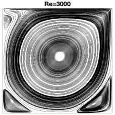
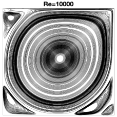
Figure 1. Shown above are streamlines of solutions found for the 2D driven cavity problems at varying Reynolds numbers.

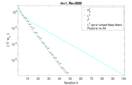
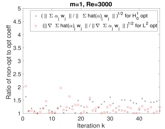
Figure 2. Shown above are residuals for the $Re$=3000 tests in the $H^{1}_{0}(\Omega)$ norm for Picard with no AA, and with AA $m=1$ with $H^{1}_{0}$, $L^{2}$, $\ell^{2}$ and diagonally lumped $L^{2}$ used in the AA optimization step (top), as well as terms that scale the linear convergence rates in the convergence theorem (bottom).

For our first test problem we use the benchmark 2D driven cavity. The setup has domain as $\Omega=(0,1)^{2}$, $f=0$, homogeneous Dirichlet boundary conditions enforced on the sides and bottom, and $[1,0]^{T}$ on the top (moving lid). We test with $Re:=\nu^{-1}$, using $Re=$3000 and 10000. It is believed that the choice of $Re=$3000 satisfies the small data condition (since Picard appears to converge linearly with constant contraction ratio), but not the choice of $Re=$10000 since Picard fails to converge for this case [23]. Driven cavity solutions at these $Re$ from our tests below are shown in Figure 1, and agree well with solutions in the literature [6]. Our computations use $(P_{2},P_{1}^{disc})$ Scott-Vogelius elements on a barycenter refinement of a $h=\frac{1}{64}$ uniform triangular mesh.

We first test with $Re$=3000 using Picard, and $m=1$ AA-Picard using $H^{1}_{0}$, $L^{2}$, $\ell^{2}$ and diagonally lumped $L^{2}$ norms in the AA optimization. Results are shown in Figure 2, and we observe that as expected we get very similar convergence results whether $H^{1}_{0}$, $L^{2}$, $\ell^{2}$ or diagonally lumped $L^{2}$ are used for the AA optimization: they differ by just 1 iteration in convergence to a tolerance of $10^{-8}$, and we note that residuals from using $L^{2}$ and its approximations all lie on top of each other in the convergence plot. All 4 choices of optimization norm with AA-Picard offer a significant improvement over the case of no acceleration. The convergence is a bit smoother when the $H^{1}_{0}$ norm is used for AA optimization, but still the overall behavior is very similar for all four norms tested.

Figure 2 at the bottom shows the terms that scale the linear terms in the residual expansions in the theorems from the previous section. The optimization gain is shown in the figure at bottom left, and we calculate that $\left(\theta_{k}^{L^{2}}\theta_{k}^{H^{1}_{0}}\right)^{1/2}$ has similar geometric mean for both methods: for $L^{2}$ norm in AA optimization it is 0.87 and for $H^{1}_{0}$ it is 0.89. However, the standard deviation for the $L^{2}$ norm case is 0.184, while for the $H^{1}_{0}$ case is 0.0650; this variability in the case of $L^{2}$ norm may partially explain the slight choppiness of the convergence plot for $L^{2}$ (and the $\ell^{2}$ and diagonally lumped $L^{2}$ as well). Finally, at bottom right are the values of $L^{2}$-optimal coefficients in the $H^{1}_{0}$ objective function, and vice versa. These ratios are generally below 1.5 with geometric mean approximately 1.2 for both.

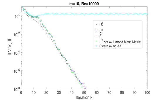
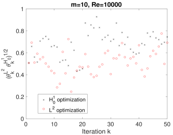
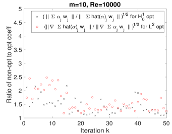
Figure 3. Shown above are residuals for the $Re$=10000 tests in the $H^{1}_{0}(\Omega)$ norm for Picard with no AA, and with AA $m=1$ with $H^{1}_{0}$, $L^{2}$, $\ell^{2}$ and diagonally lumped $L^{2}$ used in the AA optimization step (top), as well as terms that scale the linear convergence rates in the convergence theorems (bottom).

We repeat the above test for the 2D driven cavity, but now using $Re$=10000 with $m=10$ (and hence updated definitions of the gain factors that correspond to $m=10$ in the plots). Figure 3 shows convergence of the residuals, and again we observe that the overall convergence behavior of AA-Picard with $m=10$ and using $H^{1}_{0}$, $L^{2}$, $\ell^{2}$ and diagonally lumped $L^{2}$ norms in the AA optimization give very similar results, with $L^{2}$ and $\ell^{2}$ giving indistinguishable results in the plot, and diagonally lumped $L^{2}$ also indistinguishable until the residual was below $10^{-5}$ and then it differed only slightly. For the case of Picard (without AA), the iteration fails to converge.

Figure 3 at bottom shows plots of the terms that scale the linear terms in the analytical convergence estimates of the theorems of the previous section. The optimization gain terms are lower for the $m=10$ case compared to $m=1$, since it is a larger space for the optimization. The gains are somewhat better for the case of $L^{2}$ norm in the AA optimization compared to $H^{1}_{0}$. However, the ratio loss term (bottom right) for the $L^{2}$ norm for the AA optimization case, which appears to cancel out the improvement over $H^{1}_{0}$ case in the optimization gain.

4.2. 2D channel flow past a block

For our second experiment, we test AA-Picard with different choices of AA optimization norm on channel flow past a block. Several studies on this test can be found in the literature, e.g. [33, 25, 28], and it is an interesting test because the corners create reduced regularity in the flow, which can cause sensitivity in nonlinear solvers. The domain is a $2.2\times 0.41$ rectangular channel, with a square ‘block’ of side length $0.1$ with center at $(0.2,0.2)$ (with the origin set as the bottom left corner of the rectangle), see Figure 4.

Figure 4. Shown above is the channel flow past a block domain.

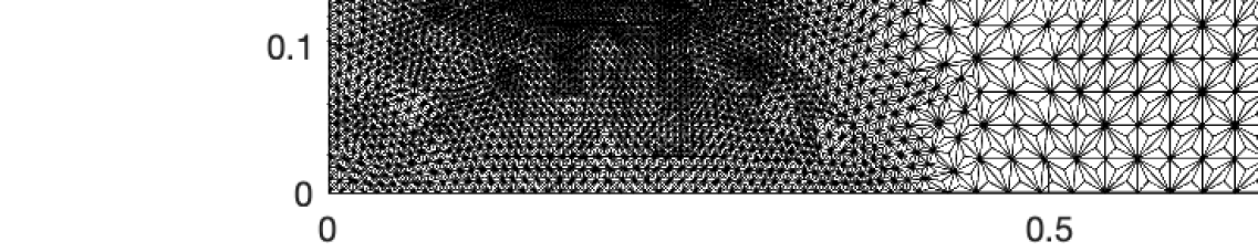
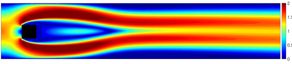
Figure 5. Shown above is (top) the mesh used for the 2D flow past a block, before the barycenter refinement, and (bottom) a plot of the speed contours of the $Re$=150 solution.

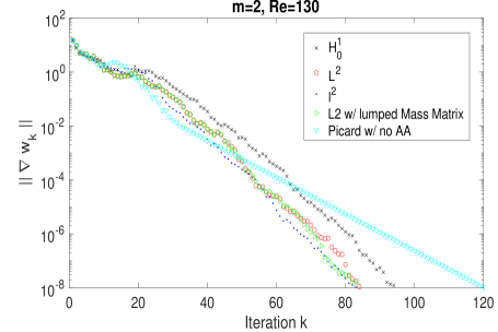
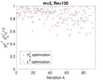
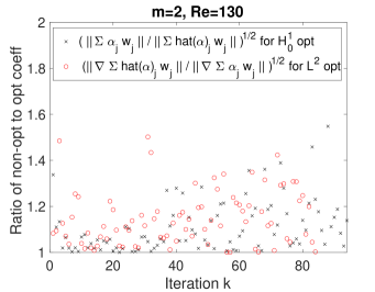
Figure 6. Shown above is the (top) convergence for Re=130 channel flow past a block, for various solvers, (bottom left) the effective gain factors for the tests using $H^{1}_{0}$ and $L^{2}$ AA optimization, and (bottom right) the ratio loss terms from using non-optimal coefficients.

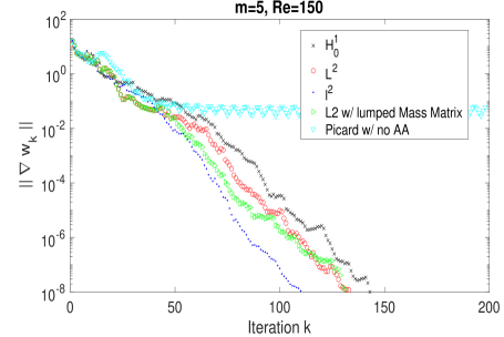
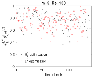
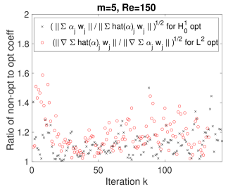
Figure 7. Shown above is the (top) convergence for Re=150 channel flow past a block, for various solvers, (bottom left) the effective gain factors for the tests using $H^{1}_{0}$ and $L^{2}$ AA optimization, and (bottom right) the ratio loss terms from using non-optimal coefficients.

No-slip velocity boundary conditions are imposed on the walls and on the block, and at the inflow the profile is set as

$$u_{1}(0,y,t)= u_{1}(2.2,y,t)=\frac{6}{0.41^{2}}y(0.41-y),$$

(4.1) $$u_{2}(0,y,t)= u_{2}(2.2,y,t)=0.$$

The outflow weakly enforces a zero traction (i.e. do nothing) Neumann boundary condition. This problem has no external forcing, $f=0$.

We compute with Reynolds numbers $Re$=130 and 150, which translates to $\nu=\frac{1}{1300}$ and $\frac{1}{1500}$ using the Reynolds length scale as the width of the block (L=0.1) and the max inflow is 1. We note that many numerical tests have been run using $Re=100$ and above for this test problem [33, 25, 28] and it is known that this test problem admits periodic-in-time solutions for these $Re$. Still, we search for (and find) steady solutions at these Reynolds numbers.

We compute using a mesh refined towards the left half of the channel and then refined again around the block, and finally refined again with a barycenter refinement over the entire mesh; the mesh is shown in Figure 5. We compute using $(P_{2},P_{1}^{disc})$ Scott-Vogelius elements, which provides 133K velocity degrees of freedom (dof) and 99K pressure dof. We test using $m=2$ for $Re$=130 and $m=5$ for $Re$=150, using $H^{1}_{0}$, $L^{2}$, $\ell^{2}$ and diagonally lumped $L^{2}$ norms for the AA optimization. Results are shown for $Re$=130 in Figure 6, and for $Re$=150 in Figure 7. For $Re$=130, we observe that convergence results for the case of $L^{2}$, $\ell^{2}$ and diagonally lumped $L^{2}$ all display very similar convergence, with $H^{1}_{0}$ coming in slightly worse (needing 10 extra iterations to converge, although its overall slope matches those with other choices of optimization norms). All choices of optimization norm provided much better convergence than Picard alone which needed 120 total iterations to converge. Similar convergence behavior is observed with $Re$=150 in Figure 7, this time with $\ell^{2}$ doing slightly better than the other choices of AA optimization norm, but here Picard alone failed to converge. In both $Re$=130 and 150 cases, there were no significant differences in the plots of terms scaling the linear convergence rates for the cases of $L^{2}$ and $H^{1}_{0}$ norms in the AA optimization, so plots are omitted.

4.3. 3D driven cavity

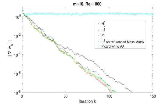
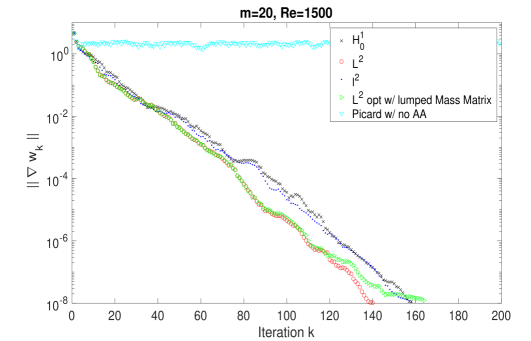
Figure 8. Shown above are convergence plots for the 3D driven cavity tests with varying choice of AA optimization norm, for $Re$=1000 (top) and $Re$=1500 (bottom).

Our final test is for the 3D lid-driven cavity problem, which is a benchmark 3D analogue of the 2D driven cavity test above. The domain is the unit cube, there is zero forcing ($f=0$), homogeneous Dirichlet boundary conditions are strongly enforced on the walls and $u=[1,0,0]^{T}$ is enforced at the top to represent the moving lid. The viscosity is chosen as the inverse of the Reynolds number, and we will use $Re$=1000 and 1500 for these tests.

We compute using a mesh first created using Chebychev points on [0,1] to construct a 14$\times$14$\times$14 grid of rectangular boxes. Each box is then split into 6 tetrahedra, and then an additional barycenter refinement splits each of these into 4 tetrahedra. $(P_{3},P_{2}^{disc})$ Scott-Vogelius elements are used, which provides approximately 1.3 million total degrees of freedom. It is known from [37] that this element choice is inf-sup stable. Solution plots found with this discretization matched those from the literature [35, 7, 19], and are shown in Figure 9.

$Re$=1000

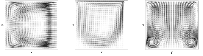
$Re$=1500

 
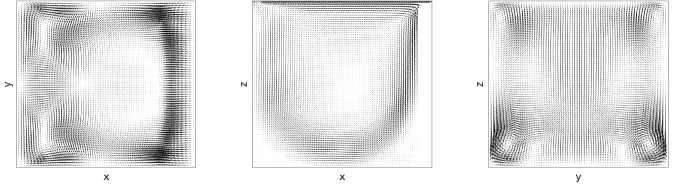
$Re$=1000                  $Re$=1500

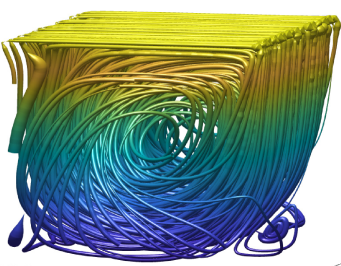
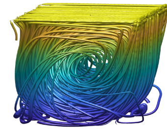
Figure 9. Shown above are solution plots for the 3D driven cavity problem with $Re$=1000 and 1500, as streamlines in the midsliceplanes of the box and as streamtubes.

Convergence results for $Re$=1000 with $m=10$ and $Re$=1500 with $m=20$ are shown in Figure 8. Once again we observe that the choices of $H^{1}_{0}$, $L^{2}$, $\ell^{2}$ and diagonally lumped $L^{2}$ all have similar convergence behavior, with $H^{1}_{0}$ being slightly worse for the case of $Re$=1000. For both $Re$=1000 and 1500, Picard alone failed to converge. As in previous tests, $L^{2}$ and diagonally lumped $L^{2}$ optimization norm tests gave nearly indistinguishable results until the residual was below $10^{-5}$.

5. Conclusions and future directions

This study investigated the effect of the choice of optimization norm in the AA-Picard iteration, in particular whether $L^{2}$ (and its more efficient approximations) provides similar convergence behavior as $H^{1}_{0}$. The reason for this is that in the HPC setting it is inefficient to use $H^{1}_{0}$, even though the convergence theory of [23] suggests that the $H^{1}_{0}$ norm should be used for the AA optimization. It is known from [36] that the right choice of norm can be critical for obtaining good convergence when enhancing a nonlinear solver with AA, and thus one should choose the norm based on mathematical reasoning.

We developed new convergence estimates, sharpening those in [23], that show similar convergence behavior is obtained for the AA-Picard solver for the NSE for the cases of $H^{1}_{0}$ and $L^{2}$ being used for the AA optimization norm. The key to the new analysis was a sharper estimate of the nonlinear terms than that given in the original proof from [23] when the $H^{1}_{0}$ norm is used for the AA optimization norm, and then recognizing that essentially the same estimate can be obtained when the $L^{2}$ norm is used.

Moreover, we found numerically that very similar convergence behavior was obtained for both $H^{1}_{0}$ norm and $L^{2}$ norm cases, on 3 benchmark tests. Further, approximations of the $L^{2}$ norm with $\ell^{2}$ and diagonally lumped $L^{2}$ norms give results very similar to those of $L^{2}$ in all cases, and in particular diagonally lumped $L^{2}$ convergence results were indistinguishable until the residual fell below $10^{-5}$ on all tests. As both the diagonally lumped $L^{2}$ and $\ell^{2}$ choices of AA optimization norm are efficient in the HPC setting, our analysis and numerical tests allows us to conclude that practitioners can confidently use either the $\ell^{2}$ or diagonally lumped $L^{2}$ norms for the optimization in the AA-Picard iteration.

The key to our analysis and showing that these particular norms will give similar convergence results was the treatment of the NSE nonlinear terms. This suggests these results may be problem specific, and even though we expect the results to extend (in an analogous fashion) to coupled NSE problems like Boussinesq and MHD, we do not at this point expect these results on choosing the $L^{2}$ norm or one of its approximations instead of the associated Hilbert space norm to necessarily extend to general nonlinear fixed point iterations.

6. Acknowledgement

Author EH was supported in part by NSF DMS 1522191. Author LR was supported in part by Department of Energy grant DE-SC0025292.

References

- [1] P. Africa, D.Arndt, W. Bangerth, B. Blais, M. Fehling, Rene Gassmoller, T. Heister, L. Heltai, M. Kronbichler, M. Maier, P. Munch, M. Schreter-Fleischhacker, J. P. Thiele, B. Turcksin, D. Wells, and V. Yushutin, The deal.II Library, Version 9.6, Journal of Numerical Mathematics, 32 (2024), pp. 369–380.
- [2] D. G. Anderson, Iterative procedures for nonlinear integral equations, J. Assoc. Comput. Mach., 12 (1965), pp. 547–560.
- [3] D. Arnold and J. Qin, Quadratic velocity/linear pressure Stokes elements, in Advances in Computer Methods for Partial Differential Equations VII, R. Vichnevetsky, D. Knight, and G. Richter, eds., IMACS, 1992, pp. 28–34.
- [4] S. Balay, S. Abhyankar, M.F. Adams, S. Benson, J. Brown, P. Brune, K. Buschelman, E.M. Constantinescu, L. Dalcin, A. Dener, V. Eijkhout, J. Faibussowitsch, W.D. Gropp, V. Hapla, T. Isaac, P. Jolivet, D. Karpeev, D. Kaushik, M.G. Knepley, F. Kong, S. Kruger, D.A. May, L. Curfman McInnes, R.Tran Mills, L. Mitchell, T. Munson, J.E. Roman, K. Rupp, P. Sanan, J. Sarich, B.F. Smith, S. Zampini, H. Zhang, H. Zhang, and J. Zhang, PETSc Web page. https://petsc.org/, 2024.
- [5] T. Charnyi, T. Heister, M. Olshanskii, and L. Rebholz, On conservation laws of Navier-Stokes Galerkin discretizations, Journal of Computational Physics, 337 (2017), pp. 289–308.
- [6] E. Erturk, T. C. Corke, and C. Gökcöl, Numerical solutions of 2d-steady incompressible driven cavity flow at high Reynolds numbers, Int. J. Numer. Methods Fluids, 48 (2005), pp. 747–774.
- [7] C. Evans, S. Pollock, L. Rebholz, and M. Xiao, A proof that Anderson acceleration improves the convergence rate in linearly converging fixed-point methods (but not in those converging quadratically), SIAM Journal on Numerical Analysis, 58 (2020), pp. 788–810.
- [8] D. J. Gardner, D. R. Reynolds, C. S. Woodward, and C. J. Balos, Enabling new flexibility in the SUNDIALS suite of nonlinear and differential/algebraic equation solvers, ACM Transactions on Mathematical Software (TOMS), (2022).
- [9] P. Guven Geredeli, L. Rebholz, D. Vargun, and A. Zytoon, Improved convergence of the Arrow-Hurwicz iteration for the Navier-Stokes equation via grad-div stabilization and Anderson acceleration, Journal of Computational and Applied Mathematics, 422 (2023), pp. 1–16.
- [10] V. Girault and P.-A. Raviart, Finite element methods for Navier–Stokes equations: Theory and algorithms, Springer-Verlag, 1986.
- [11] J. Guzman and L.R. Scott, The Scott-Vogelius finite elements revisited, Math. Comp., 88 (2019), pp. 515–529.
- [12] J. Heywood and R. Rannacher, Finite element approximation of the nonstationary Navier-Stokes problem. Part I: Regularity of the solution and second order estimates for spatial discretization, SIAM J. Numer. Anal., 19(2) (1982), pp. 353–384.
- [13] S. Ingimarson, Advancements in fluid simulation through enhanced conservation schemes, Ph.D. thesis, Clemson University, (2023).
- [14] V. John, A. Linke, C. Merdon, M. Neilan, and L. G. Rebholz, On the divergence constraint in mixed finite element methods for incompressible flows, SIAM Review, 59 (2017), pp. 492–544.
- [15] C.T. Kelley, Numerical methods for nonlinear equations, Acta Numerica, 27 (2018), pp. 207–287.
- [16] W. Layton, An Introduction to the Numerical Analysis of Viscous Incompressible Flows, SIAM, Philadelphia, 2008.
- [17] J. Liu, L. Rebholz, and M. Xiao, Efficient and effective algebraic splitting iterations for nonlinear saddle point problems, Mathematical Methods in the Applied Sciences, 47 (2024), pp. 451–474.
- [18] M. Mohebujjaman, M. Xiao, and C. Zhang, A simple-to-implement nonlinear preconditioning of Newton’s method for solving the steady Navier-Stokes equations, Submitted, (2025).
- [19] S. Pollock and L. Rebholz, Anderson acceleration for contractive and noncontractive operators, IMA Journal of Numerical Analysis, 41 (2021), pp. 2841–2872.
- [20] , Filtering for Anderson acceleration, SIAM Journal on Scientific Computing, 45 (2023), pp. A1571–A1590.
- [21] , Anderson Acceleration for Numerical PDEs, SIAM, Philadelphia, 2025.
- [22] S. Pollock, L. Rebholz, X. Tu, and M. Xiao, Analysis of the Picard-Newton iteration for the Navier-Stokes equations: global stability and quadratic convergence, Journal of Scientific Computing, in press (2025).
- [23] S. Pollock, L. Rebholz, and M. Xiao, Anderson-accelerated convergence of Picard iterations for incompressible Navier-Stokes equations, SIAM Journal on Numerical Analysis, 57 (2019), pp. 615– 637.
- [24] L. Rebholz, D. Vargun, and M. Xiao, Enabling fast convergence of the iterated penalty Picard iteration with penalty parameter for incompressible Navier-Stokes via Anderson acceleration, Computer Methods in Applied Mechanics and Engineering, 387 (2021), pp. 1–17.
- [25] W. Rodi, Comparison of LES and RANS calculations of the flow around bluff bodies, Journal of Wind Engineering and Industrial Aerodynamics, 69-71 (1997), pp. 55–75. Proceedings of the 3rd International Colloqium on Bluff Body Aerodynamics and Applications.
- [26] Y. Saad, Acceleration methods for fixed point problems, Acta Numerica, (2024), pp. 1–85.
- [27] M. Schfer and S. Turek, The benchmark problem ‘flow around a cylinder’ flow simulation with high performance computers II, in E.H. Hirschel (Ed.), Notes on Numerical Fluid Mechanics, 52, Braunschweig, Vieweg (1996), pp. 547–566.
- [28] A. Sohankar, L. Davidson, and C. Norberg, Large Eddy Simulation of Flow Past a Square Cylinder: Comparison of Different Subgrid Scale Models , Journal of Fluids Engineering, 122 (1999), pp. 39–47.
- [29] H. De Sterck and Y. He, Linear asymptotic convergence of Anderson acceleration: fixed point analysis, SIAM Journal on Matrix Analysis and Applications, 43 (2022).
- [30] H. De Sterck, Y. He, and O. Krzysik, Anderson acceleration as a Krylov method with application to convergence analysis, Journal of Scientific Computing, 99 (2024).
- [31] R. Temam, Navier-Stokes equations, Elsevier, North-Holland, 1991.
- [32] A. Toth and C. T. Kelley, Convergence analysis for Anderson acceleration, SIAM J. Numer. Anal., 53 (2015), pp. 805–819.
- [33] F.X. Trias, A. Gorobets, and A. Oliva, Turbulent flow around a square cylinder at Reynolds number 22,000: A DNS study, Computers & Fluids, 123 (2015), pp. 87–98.
- [34] H. F. Walker and P. Ni, Anderson acceleration for fixed-point iterations, SIAM J. Numer. Anal., 49 (2011), pp. 1715–1735.
- [35] K.L. Wong and A.J. Baker, A 3d incompressible Navier-Stokes velocity-vorticity weak form finite element algorithm, International Journal for Numerical Methods in Fluids, 38 (2002), pp. 99–123.
- [36] Y. Yang, A. Townsend, and D. Appelö, Anderson acceleration based on the H-s Sobolev norm for contractive and noncontractive fixed-point operators, Journal of Computational and Applied Mathematics, 403 (2022), p. 113844.
- [37] S. Zhang, A new family of stable mixed finite elements for the 3d Stokes equations, Math. Comp., 74 (2005), pp. 543–554.