Markov Modelling Approach for Queues with Correlated Service Times — the $M/M_{D}/2$ Model

Abstract

Demand for studying queueing systems with multiple servers providing correlated services was created about 60 years ago, motivated by various applications. In recent years, the importance of such studies has been significantly increased, supported by new applications of greater significance to much larger scaled industry, and the whole society. Such studies have been considered very challenging. In this paper, a new Markov modelling approach for queueing systems with servers providing correlated services is proposed. We apply this new proposed approach to a queueing system with arrivals according to a Poisson process and two positive correlated exponential servers, referred to as the $M/M_{D}/2$ queue. We first prove that the queueing process (the number of customers in the system) is a Markov chain, and then provide an analytic solution for the stationary distribution of the process, based on which it becomes much easier to see the impact of the dependence on system performance compared to the performance with independent services.

1 Introduction

1.1 Motivations

The $M/M/c$ queueing system was first introduced and studied by Agner Krarup Erlang in 1909 in [9], which later becomes one of the most popular queueing systems in applications with independent servers. Since the late 1970s, queueing systems with correlated servers have been proposed and studied by several researchers, motivated by various applications.

Kleinrock realized the importance of dependent service times in message-switching communication networks (MSCN) in [15]. In MSCN, messages (customers) are divided into pieces according to channel capacity (service time) during message transmission through the network, which requires identical service times at each tandem node in queueing language. This type of network models (or tandem queues) later becomes more popular under the packet-switching technique, and is the main focus of the studies for queueing systems with dependent servers.

Mitchell et al. in [19] offered two scenarios in production lines and logistics, in which service times could be correlated: (1) in a paper mill, and (2) in the overhaul of an aircraft engine. They suggested that “An obvious approach is to use a multivariate exponential distribution with non-zero correlations in place of the usual independent exponential service times.” And they further questioned that “it is not clear that the birthdeath equation approach can be modified to incorporate dependent service times. Moreover, any such formulation would very likely be analytically intractable.”

In [10], Choo and Conolly described two situations, in which correlated service times are intuitively obvious: “That correlation may be relevant is intuitively clear from the supermarket example where most customers who spend a long time in the shopping area also ipso facto require a long checkout time. And a patient with an unknown disease may spend a long time at each of a series of investigative stages until the disease is identified, followed perhaps by long periods of treatment and convalescence.”

Two more applications of queues requiring dependent service times were provided in Pang and Whitt [21]. The first example is in a technical support telephone call center responding to service call. It is anticipated that the handling (service) times of calls, after the product with a defect is first introduced, are longer-than-usual. The other example is in a hospital emergency room. Multiple patients may be associated with the same medical incident (say a highway accident, or food poisoning at the same restaurant), all of whom require longer service times.

In recent years, new applications have been emerging, which show much bigger importance on national economy, national security, key industries, and the whole society. For example, social behaviour and decisions on policy making might be required to be included in modelling for competitions between nations or key companies in areas such as, chip manufacturing, smart phone production, AI products, on-line ordering, resource or product-sharing. All the above situations could lead to a queueing model with servers (nations, or key companies) whose service times are correlated (often positive correlated).

1.2 Literature review

Though it is important and well-motivated, the number of literature studies on queueing systems with correlated service times is still relatively small. It was believed, say by Choo and Conolly [10] and Pinedo and Wolff [23], that the work by Mitchell et al. [19] in 1977 was the first publication dealing with queueing systems with dependent service times provided by two servers in a tandem queue setting. Since then, most of studies have focused on tandem queues due to the nature of their structures. In fact, Kelly [12] in 1976 already obtained some exact results for a time-sharing queueing network in which the service times for a customer remain the same throughout the network.

In [19], the authors provided a simulation study on the impact of system performance of a two-node tandem queue with Poisson arrivals and bivariate exponential service times. They showed that the system behaviour is quite sensitive to the dependence, especially at higher utilizations, for either positive or negative correlation.

The same tandem queueing system was also studied by Hoon Choo and Conolly [10] for the positive correlated case. It was an attempt to have an analytical treatment on the waiting time. Since the waiting time at the first queue is the same as that for the standard $M/M/1$ model, only the waiting time at the second stage requires attentions. The correlation between the service times provided at the two stages can be converted to the correlation of the service time at the second stage and the interarrival times to the second queue. This observation enables the authors to apply the method used in [8] to obtain an explicit expression for the Laplace transform of the (stationary) waiting time at stage 2 (see equation (4.8) of [10]).

In Boxma [2, 3], the author also studied a two-stage tandem queue with Poisson arrivals, in which the service time at node 1 was extended from an exponential random variable (r.v.) to a r.v. with a general distribution. The dependence of the service times at the two nodes requires that each customer’s service time at node two is identical to that at node one. A comprehensive analysis of this model was carried out by the author, which leads to explicit (not in transformation form) expressions for the stationary sojourn time and waiting time. This work provided answers to an open problem that was proposed but remained unanswered in Kleinrock [15]. The analysis in [2] was based on queueing model dynamics through a combination of multiple queue techniques, such as transformation and imbedded. Computational implementations were addressed in [3]. For the same model, Boxma and Deng [4] obtained asymptotic results for delay distributions in the case of regularly varying service times, and also in heavy traffic conditions. In the book [13], Kelly also considered networks of symmetric queues allowing dependent service times.

In two IBM technical reports [6, 7], Calo obtained an expression for the Laplace-Stieltjes transform for the stationary distribution of the total waiting time of a customer in a tandem queue of multiple stages with a general arrival and general, but equal, service times.

Pinedo and Wolff [23] considered Markovian tandem queues of $m$ stages (Poisson arrivals and exponential service times), in which each given customer has the equal (random) service time at each stage. For $m=2$ model with infinite waiting capacity of queues, they obtained bounds (upper or lower) on the total expected time for a customer in both queues when the two service times (with equal mean) are NBUE or NWUE. For the tandem queue of $m\geq 2$ with no waiting space between queues (or blocking case) they considered the system throughput $\lambda_{\sup}(D)$ for the dependent case, which was compared with the throughput $\lambda_{\sup}(I)$ for the independent case. It was proved that for $m>2$, $\lambda_{\sup}(D)<\lambda_{\sup}(I)$. Properties on stochastic ordering were used for obtaining the above results. The work on the throughput in [23] for the blocking case was extended for the non-blocking case by Browning [5], who proved that for a general $m$, when the waiting space between stages is large enough the reverse inequality for the throughput $\lambda_{\mbox{sup}}(D)>\lambda_{\mbox{sup}}(I)$ holds.

Kelly [14] considered a series of nodes (queues) with a finite buffer between two consecutive nodes for transmitting messages. The lengths of successive messages are assumed to be i.i.d. random variables. The author obtained the rate at which buffer sizes need to increase in order to maintain the system throughput as the number $n$ of nodes increases.

Light traffic asymptotics for the expected delay in a series of $r\geq 2$ queues with correlated service times was investigated in Wolff [28]. For $r=2,3$, the study applies to an arbitrary correlated joint distribution of service times, but for $r>3$, conclusions were made for equal service times.

Ziedins [29] also considered a tandem queueing system with a finite waiting capacity between two consecutive nodes, where any given customer has the same service time at each of the nodes. The author showed that, in terms of service time distributions with only two support points, it is always optimal to allocate the capacity as uniformly as possible, even when blocking occurs, which is different from the earlier suggestions in the literature.

Avi-Itzhak and Levy [1] considered tandem queues with deterministically correlated service times.

For tandem queues and through simulations results, in Sandmann [24], different types of correlations, including equal service times, were considered for the two node case with exponential and uniform service times at the first node. Later, Sandmann [26] considered the end-to-end delay with correlated service times, which is a continuation of his earlier work [25]. Specifically, the service time at the first node is a random variable, and the service time at any other node is correlated with that at the first node.

Pang and Whitt explored heavy traffic approximations under a different setting of queue models with dependent service times. Specifically, (a) in [22] (and also in [21]), an infinite-server queue, denoted by $G_{t}/G^{D}/\infty$, was considered, where the arrival process was assumed to satisfy a functional central limit theorem (FCLT), and the successive service times were assumed to be weakly dependent in the sense that the dependence among the service times is limited so that the CLT remains valid, but the variability constant in the CLT is affected by the cumulative correlations. For such a system, heavy-traffic limits, including a functional weak law of large numbers (FWLLN) and an FCLT were obtained; and (b) in [20], the work in [22] was extended to a generalized model allowing batch arrivals, denoted by $G_{t}^{B}/G^{D}/\infty$, in which dependent service times are restricted for customers in the same batch. In [20], two special dependent service times, multivariate Marshall–Olkin (MO) exponential distributions and multivariate MO hyperexponential distributions within a batch were adopted for illustrating general results.

1.3 Main contributions in this paper

The main contribution made in this paper is the proposal of a new approach for studying queueing systems with correlated servers, say the $M/M_{D}/2$ model. This new approach addresses a long-standing open concern raised in [19] (see also Section 1.1 on motivations). With our new approach, the birth-death equation approach indeed can be extended to deal with queueing systems with dependent service times. To prove the queueing process is actually a Markov chain, special cares have to be taken, including the dependent service rate, and the simultaneous departures from both servers due to singularities in the service time (see Theorem 1 and Corollary 3.1). It is worthwhile to point out that the Markov chain is no longer a birth-and-death process as in the case of independent servers. However, the stationary distribution is still geometric (see Theorem 2 and Corollary 4.3), which ensures that our formulation is indeed analytically tractable.

1.4 Organization of the paper

Following the introduction section, the rest of the paper is organized as follows: in Section 2, we provide some literature results, which are required in our study, including the concept of 2-dimensional lack-of-memory property, and Marshall-Olkin bivariate exponential (MO-BVE) distribution and its properties; in Section 3, we introduce the $M/M_{D}/2$ queueing system and define the queueing process of this system. We prove that the queueing process of the $M/M_{D}/2$ system is a Markov chain; in Section 4, we provide the stationary solution of the Markov chain for the $M/M_{D}/2$ system, which is geometric with modified solutions at the boundary states; in Section 5, based on the main results obtained in previous sections, we demonstrate the impact of the dependence between the servers on the system performance; and in the last section, Section 6, concluding remarks are made.

2 Bivariate dependent service times

Recall that the focus of this paper is to propose a Markovian model to study multi-server queues with dependent service times, in a similar fashion as $M/M/c$ was proposed to study multi-server queues with independent service times. In the case of the standard $M/M/c$ queue, the number of customers in the system at time $t$ is a Markov chain, proved based on the lack-of-memory property of the exponential random variable (r.v.). A univariate non-negative continuous r.v. $X$ is called lack-of-memory, if it satisfies the following property:

$$P(X>t+x|X>x)=P(X>t),\quad\text{for all $x,t\geq 0$.}$$

It is well-known that the exponential r.v. is the unique continuous non-negative r.v. satisfying the above lack-of-memory property.

In the literature, extending the lack-of-memory concept to multi-variate r.v.s was started from the seminal work by Marshall and Olkin [18], and has been since a central topic in multi-variate distributions. References on this topic are vast, and besides [18] we only mention Kots et al. [16] and Lin et al. [17] since all we need in our analysis can be conveniently found in these references. The lack-of-memory concept, in both strong and weak senses, and their properties introduced in this section are all literature results.

For the case of two r.v.s, it is intuitive to extend the lack-of-memory property to:

$$P(X>x+s,Y>y+t|X>s,Y>t)=P(X>x,Y>y),$$

which is equivalent to, in terms of the survival function $\bar{H}$,

$$\bar{H}(x+s,y+t)=\bar{H}(x,y)\bar{H}(s,t),\quad\text{all $x,y,s,t\geq 0$,}$$

where $H$ is the distribution function of $(X,Y)$ and $\bar{H}=1-H$. However, the above equation has only one solution, in which $X$ and $Y$ are independent exponential r.v.s. Therefore, lack-of-memory in weak sense has been proposed: $(X,Y)$ satisfies the bivariate lack-of-memory (BLM) property if

$$\bar{H}(x+t,y+t)=\bar{H}(x,y)\bar{H}(t,t),\quad\text{all $x,y,t\geq 0$.}$$

Lack-of-memory in weak sense is equivalent to:

$$P(X>x+t,Y>y+t|X>t,Y>t)=P(X>x,Y>y),\quad\text{all $x,y,t\geq 0$,}$$

(see, for example, equation (2.7) in [18]), which is more often used for the context of reliability in the literature. Unfortunately, the above expression, in terms of a conditional probability, is not a convenient form in our analysis for proving that the queueing process is a Markov chain. Instead, we use another equivalent form:

$$P(X>x+t,Y>y+t|X>x,Y>y)=P(X>t,Y>t),\quad\text{all $x,y,t\geq 0$,}$$ (2.1)

(see, for example, equation (2.9) in [18]).

In our case, to have a Markov chain model, it is required that the marginal distributions are exponential (dealing with the case when one server is idle). Under this requirement (exponential marginals), it is well-known that the Marshall-Olkin bivariate exponential (MO-BVE) distribution is the only solution, which satisfies the lack-of-memory property in weak sense.

Definition 2.1

A bivariate distribution is called MO-BVE with parameters $\mu_{1}\geq 0$, $\mu_{2}\geq 0$ and $\mu_{12}\geq 0$, if its survival function $\bar{H}$ is given by

$$\bar{H}(x,y)=e^{-(\mu_{1}x+\mu_{2}y+\mu_{12}\max(x,y))},\quad x,y\geq 0,$$ (2.2)

For the MO-BVE distribution, we provide a summary of its properties, which are needed in our analysis.

Properties 1

For the bivariate r.v.s $(X,Y)$ having the MO-BVE distribution, the following properties hold:

(1)

The MO-BVE distribution is the only distribution satisfying the BLM property in weak sense (see, for example, equation (2.1)), if the two marginal distributions are required to be exponential;

(2)

The density function $f$ of MO-BVE r.v.s $(X,Y)$ (or variables $(X,Y)$ having the MO-BVE distribution) is given by

$$f(x,y)=\left\{\begin{array}[]{ll}\mu_{2}(\mu_{1}+\mu_{12})\bar{H}(x,y),&\mbox{for }0<y<x,\\ \mu_{1}(\mu_{2}+\mu_{12})\bar{H}(x,y),&\mbox{for }0<x<y,\\ \mu_{12}\bar{H}(z,z),&\mbox{for }x=y=z>0;\end{array}\right.$$ (2.3)

or

$$f(x,y)=\left\{\begin{array}[]{ll}\mu_{2}(\mu_{1}+\mu_{12})e^{-(\mu_{1}+\mu_{12})x+\mu_{2}y},&\mbox{for }0<y<x,\\ \mu_{1}(\mu_{2}+\mu_{12})e^{-(\mu_{2}+\mu_{12})y+\mu_{1}x},&\mbox{for }0<x<y,\\ \mu_{12}e^{-(\mu_{1}+\mu_{2}+\mu_{12})z},&\mbox{for }x=y=z>0.\end{array}\right.$$ (2.4)

See, for example, equation (47.51) in [16]. It is worthwhile to note that the MO-BVE distribution is singular on $X=Y$ since $P(X=Y)>0$;

(3)

The marginal distributions of $X$ and $Y$ are both exponential with rates $\mu_{1}+\mu_{12}$ and $\mu_{2}+\mu_{12}$, respectively:

$$X\sim\exp(\mu_{1}+\mu_{12});\quad Y\sim\exp(\mu_{2}+\mu_{12}).$$ (2.5)

(4)

Based on (2.4), we have

$$P(X=Y>t)=\frac{\mu_{12}}{\mu_{1}+\mu_{2}+\mu_{12}}e^{-(\mu_{1}+\mu_{2}+\mu_{12})t},\quad t\geq 0,$$ (2.6)

and

$$P(X=Y)=\frac{\mu_{12}}{\mu_{1}+\mu_{2}+\mu_{12}};$$ (2.7)

(5)

Based on the survival function $\bar{H}$, it is easy to get that the minimum of $X$ and $Y$ is exponential with rate $\mu_{1}+\mu_{2}+\mu_{12}$:

$$\min(X,Y)\sim\exp(\mu_{1}+\mu_{2}+\mu_{12});$$ (2.8)

(6)

The correlation coefficient $\rho_{X,Y}$ between $X$ and $Y$ is given by

$$\rho_{X,Y}=\frac{\mu_{12}}{\mu_{1}+\mu_{2}+\mu_{12}}.$$

It is worthwhile to note that the MO-BVE r.v.s can only be a model for service times with positive dependence;

(7)

The conditional density $f_{Y|X}(y|x)$ of $Y$ given $X$ is given by

$$f_{Y|X}(y|x)=\left\{\begin{array}[]{ll}\frac{\mu_{1}(\mu_{2}+\mu_{12})}{\mu_{1}+\mu_{12}}e^{-(\mu_{2}+\mu_{12})y+\mu_{12}x},&\mbox{for }y>x,\\ \mu_{2}e^{-\mu_{2}x},&\mbox{for }y<x.\end{array}\right.$$ (2.9)

Symmetrically, we have

$$f_{X|Y}(x|y)=\left\{\begin{array}[]{ll}\frac{\mu_{2}(\mu_{1}+\mu_{12})}{\mu_{2}+\mu_{12}}e^{-(\mu_{1}+\mu_{12})x+\mu_{12}y},&\mbox{for }x>y,\\ \mu_{1}e^{-\mu_{1}x},&\mbox{for }x<y.\end{array}\right.$$ (2.10)

See equation (47.52) in [16] for more information;

(8)

$P(X<Y)=\mu_{1}/(\mu_{1}+\mu_{2}+\mu_{12})$.

3 The $M/M_{D}/2$ model

In this section, we propose a new queueing model, that can be considered a generalization of the $M/M/c$ queue for $c=2$, denoted by $M/M_{D}/2$, where $M_{D}$ is used to emphasize that the service times provided by the two servers can be dependent. Specifically, this is a queueing system with a waiting space of infinite capacity, where the arrivals to this system follow a Poisson process, independent of service times, with rate $\lambda$, and the service times provided by the two servers follow the MO-BED, given by (2.4), where $\lambda_{1}=\mu_{1}+\mu_{12}$ and $\lambda_{2}=\mu_{2}+\mu_{12}$ are the marginal exponential service rates of server 1 and server 2, respectively, and $\mu_{12}$ is the dependent parameter.

Define the state to be the number of customers in the system. The state space $S$ is defined as

$$S=\{0,(1,0),(0,1),2,3,\ldots\},$$ (3.1)

where state $n$, for $n=0$ and $n\geq 2$, represents the number of customers in the system, and states $(1,0)$ and $(0,1)$ represent only one customer in the system, being served by server 1 and 2, respectively.

An arrival to the empty system would change the state to $(1,0)$ with probability $0\leq p\leq 1$, or to $(0,1)$ with probability $q=1-p$; an arrival to state $(1,0)$ or $(0,1)$ changes the state to $2$; and an arrival to state $n$ for $n\geq 2$ changes the state to $n+1$. When the system is not empty, the service time of the customer or the two customers in the service is characterized by the MO-BED. After a service completion, the customer departs from the system, bringing the number of customers in the system down by one. Let $X(t)$ be the number of customers in the system at time $t$. We will show in the next section that $\{X(t):t\geq 1\}$ is a Markov chain.

It is our expectation that this new queueing system can be used as a mathematical model for applications, in which service times are positively correlated. We hope that this basic system can play a role in modelling queueing systems with dependent servers, similar to the role played by the $M/M/c$ queueing for systems with independent servers.

Remark 3.1

Since the marginal service rates are different in general, we cannot use 1 to represent the state of one customer in the system. Instead, in this case, we need to specify which server is busy using $(1,0)$ or $(0,1)$. This definition of the state space was also used in modelling the $M/M/2$ queueing system with two heterogeneous servers (for example, see [11] and [27]).

3.1 Markov chain

In this section, we prove that the process $X(t)$ defined in the previous section with state space $S$ specified in (3.1) is a Markov chain. It is worth noting that modelling a queueing system with dependent service times as a Markov chain is a new approach proposed in this paper. With this Markov chain, we hope many classical methods applied to queueing systems with independent service times can be extended to queueing systems with dependent service times.

Theorem 1

For the $M/M_{D}/2$ queueing system with arrival rate $\lambda$ and two heterogeneous dependent servers characterized by the MO-BED with parameters $\mu_{1}$, $\mu_{2}$ and $\mu_{12}$ given in (2.4), the process $\{X(t):t\geq 0\}$ defined in the previous section, representing the number of customers in the system at time $t$, is a continuous time Markov chain with transition rate matrix $Q=(q_{i_{1},i_{2}})$ given by:

$$Q=\hbox{}\;\vbox{\kern 86.55554pt\hbox{$\kern 336.12584pt\kern-8.75pt\left[\kern-336.12584pt\vbox{\kern-86.55554pt\vbox{\halign{$#$\hfil\kern 2\p@\kern\@tempdima& \thinspace\hfil$#$\hfil&& \quad\hfil$#$\hfil\cr\hfil\crcr\kern-12.0pt\cr$\hfil\kern 2.0pt\kern 8.75pt&0&(1,0)&(0,1)&2&3&4&5&6&\cdots&&\crcr\kern 2.0pt\cr 0$\hfil\kern 2.0pt\kern 8.75pt&-\lambda&p\lambda&q\lambda&\cr\hskip-8.53581pt(1,0)$\hfil\kern 2.0pt\kern 8.75pt&\mu_{1}+\mu_{12}&-\theta_{(1,0)}&0&\lambda&\cr\hskip-8.53581pt(0,1)$\hfil\kern 2.0pt\kern 8.75pt&\mu_{2}+\mu_{12}&0&-\theta_{(0,1)}&\lambda&\cr 2$\hfil\kern 2.0pt\kern 8.75pt&\mu_{12}&\mu_{2}&\mu_{1}&-\theta&\lambda&\cr 3$\hfil\kern 2.0pt\kern 8.75pt&&p\mu_{12}&q\mu_{12}&\mu_{1}+\mu_{2}&-\theta&\lambda&\cr 4$\hfil\kern 2.0pt\kern 8.75pt&&&&\mu_{12}&\mu_{1}+\mu_{2}&-\theta&\lambda&\cr 5$\hfil\kern 2.0pt\kern 8.75pt&&&&&\mu_{12}&\mu_{1}+\mu_{2}&-\theta&\lambda&\cr\vdots$\hfil\kern 2.0pt\kern 8.75pt&&&&&&\ddots&\ddots&\ddots&\ddots\crcr\cr}}\kern-12.0pt}\,\right]$}},$$ (3.2)

where all empty entries are 0, $\theta_{(1,0)}=\lambda+\mu_{1}+\mu_{12}$, $\theta_{(0,1)}=\lambda+\mu_{2}+\mu_{12}$, $\theta=\lambda+\mu_{1}+\mu_{2}+\mu_{12}$, and $0<p<1$ with $q=1-p$.

Proof. We divide the proof into two steps: in the first step, we show that the sojourn time in each state is exponential with the parameter dependent on the current state (independent of the future state); and in the second step, we explicitly derive the transition probabilities for the imbedded Markov chain.

Step 1.

State 0: For $i=0$,

$$\mbox{sojourn time in 0}=\mbox{remaining interarrival time}=A\sim\exp(\theta_{0}),$$

where $A$ is the interarrival time and $\theta_{0}=\lambda$.

State (1,0): For state $(1,0)$,

sojourn time in $$(1,0) =\min(\mbox{remaining interarrival time, remaining service time at server 1)}$$

$$=\min(A,S_{1})\sim\exp(\theta_{(1,0)}),$$

where $\theta_{(1,0)}=\lambda+\mu_{1}+\mu_{12}$ since only server 1 is busy and the marginal service time $S_{1}\sim\exp(\mu_{1}+\mu_{12})$.

State (0,1): For state $(0,1)$, it can be similarly shown that

sojourn time in $$(0,1) =\min(\mbox{remaining interarrival time, remaining service time at server 2)}$$

$$=\min(A,S_{2})\sim\exp(\theta_{(0,1)}),$$

where $\theta_{(0,1)}=\lambda+\mu_{2}+\mu_{12}$ since only server 2 is busy and the marginal service time $S_{2}\sim\exp(\mu_{2}+\mu_{12})$.

State $i$: For state $i\geq 2$,

sojourn time in $$i =\min(\mbox{remaining interarrival time, remaining service times at servers 1 and 2)}$$

$$=\min(A,(S_{1},S_{2}))=\min(A,\min(S_{1},S_{2}))\sim\exp(\theta_{i}),$$

where $\theta_{i}=\lambda+\mu_{1}+\mu_{2}$ since $\min(S_{1},S_{2})\sim\exp(\mu_{1}+\mu_{2}+\mu_{12})$.

Step 2. Let $X_{n}$ be the imbedded process of $X(t)$, or $X_{n}$ is the state to which $X(t)$ moves when it makes its $n$th transition. For the model with heterogeneous servers, when a customer is arriving to an empty system, we need to specify which server the arriving customer would be sent to. We assume that with probability $p$, the process moves from 0 to $(1,0)$, and with $q=1-p$ from 0 to $(0,1)$.

State 0: When $X_{n}=0$, it follows from the above assumption that

$$p_{0,(1,0)}=p\quad\mbox{and}\quad p_{0,(0,1)}=q=1-p,$$

which are independent of past transitions.

State (1,0): When $X_{n}=(1,0)$,

$$P(X_{n+1}=0|X_{n}=(1,0)) =P(\mbox{remaining service time at server 1 $<$ remaining interarrival time})$$

$$=P(S_{1}<A)=\frac{\mu_{1}+\mu_{12}}{\lambda+\mu_{1}+\mu_{12}}=p_{(1,0),0},$$

which is independent of past transitions; and similarly

$$P(X_{n+1}=2|X_{n}=(1,0)) =P(\mbox{remaining service time at server 1 $>$ remaining interarrival time})$$

$$=P(A<S_{1})=\frac{\lambda}{\lambda+\mu_{1}+\mu_{12}}=p_{(1,0),2}.$$

State (0,1): When $X_{n}=(0,1)$, we can similarly show that

$$p_{(0,1),0}=\frac{\mu_{2}+\mu_{12}}{\lambda+\mu_{2}+\mu_{12}}\quad\mbox{and}\quad p_{(0,1),2}=\frac{\lambda}{\lambda+\mu_{2}+\mu_{12}}.$$

State 2: When $X_{n}=2$,

$$P(X_{n+1}=3|X_{n}=2) =P(A<\min(S_{1},S_{2}))$$

$$=\frac{\lambda}{\lambda+\mu_{1}+\mu_{2}+\mu_{12}}=p_{2,3},$$

which is independent of past transitions.

Note that the MO-BED is singular on $S_{1}=S_{2}$, which implies that with a positive probability we can have simultaneous service completions from both servers. Noticing that

$$P(S_{1}=S_{2}\leq t)=\frac{\mu_{12}}{\mu_{1}+\mu_{2}+\mu_{12}}\big{[}1-e^{-(\mu_{1}+\mu_{2}+\mu_{12})t}\big{]},\quad t\geq 0,$$

according to (2.6) and (2.7), which leads to the density $f_{S_{1}=S_{2}}(t)$ of $S_{1}=S_{2}$, given by

$$f_{S_{1}=S_{2}}(t)=\mu_{12}e^{-(\mu_{1}+\mu_{2}+\mu_{12})t},\quad t\geq 0.$$ (3.3)

Then, by conditioning on the value of $S_{1}=S_{2}$, we have

$$p_{2,0} =P(S_{1}=S_{2}<A)=\int_{0}^{\infty}\mu_{12}e^{-(\mu_{1}+\mu_{2}+\mu_{12})t}P(A>t|S_{1}=S_{2}=t)dt$$

$$=\int_{0}^{\infty}\mu_{12}e^{-(\mu_{1}+\mu_{2}+\mu_{12})t}P(A>t)dt$$

$$=\mu_{12}\int_{0}^{\infty}e^{-(\mu_{1}+\mu_{2}+\mu_{12})t}e^{-\lambda t}dt$$

$$=\frac{\mu_{12}}{\lambda+\mu_{1}+\mu_{2}+\mu_{12}}\int_{0}^{\infty}(\lambda+\mu_{1}+\mu_{2}+\mu_{12})e^{-(\lambda+\mu_{1}+\mu_{2}+\mu_{12})t}dt$$

$$=\frac{\mu_{12}}{\lambda+\mu_{1}+\mu_{2}+\mu_{12}}.$$

By conditioning on the value of $S_{2}$, we now calculte

$$p_{2,(1,0)} =P(\min(S_{1},S_{2})<A,S_{2}<S_{1})=P(S_{2}<A,S_{2}<S_{1})$$

$$=\int_{0}^{\infty}f_{S_{2}}(t)P(S_{2}<A,S_{2}<S_{1}|S_{2}=t)dt$$

$$=\int_{0}^{\infty}f_{S_{2}}(t)P(A>t,S_{1}>t|S_{2}=t)dt$$

$$=\int_{0}^{\infty}f_{S_{2}}(t)P(A>t|S_{2}=t)P(S_{1}>t|A>t,S_{2}=t)dt$$

$$=\int_{0}^{\infty}f_{S_{2}}(t)P(A>t)P(S_{1}>t|S_{2}=t)dt.$$

Notice that the density function $f_{S_{1}|S_{2}}(x|y)$ is given by (2.10), or

$$f_{X|Y}(x|y)=\frac{\mu_{2}(\mu_{1}+\mu_{12})}{\mu_{2}+\mu_{12}}e^{-(\mu_{1}+\mu_{12})x+\mu_{12}y},\quad\mbox{for }x>y,$$

based on which we calculate

$$P(S_{1}>t|S_{2}=t) =\int_{t}^{\infty}\frac{\mu_{2}(\mu_{1}+\mu_{12})}{\mu_{2}+\mu_{12}}e^{-(\mu_{1}+\mu_{12})x+\mu_{12}t}dx$$

$$=\frac{\mu_{2}(\mu_{1}+\mu_{12})}{\mu_{2}+\mu_{12}}e^{\mu_{12}t}\int_{t}^{\infty}e^{-(\mu_{1}+\mu_{12})x}dx$$

$$=\frac{\mu_{2}}{\mu_{2}+\mu_{12}}e^{\mu_{12}t}e^{-(\mu_{1}+\mu_{12})t}=\frac{\mu_{2}}{\mu_{2}+\mu_{12}}e^{-\mu_{1}t}.$$

Finally, by noticing that $f_{S_{2}}(t)$ is exponential with parameter $\mu_{2}+\mu_{12}$, we have

$$p_{2,(1,0)} =\int_{0}^{\infty}(\mu_{2}+\mu_{12})e^{-(\mu_{2}+\mu_{12})t}\frac{\mu_{2}}{\mu_{2}+\mu_{12}}e^{-\mu_{1}t}dt$$

$$=\frac{\mu_{2}}{\lambda+\mu_{1}+\mu_{2}+\mu_{12}}.$$

Similarly,

$$P(X_{n+1}=(0,1)|X_{n}=2) =P(\min(S_{1},S_{2})<A,S_{1}<S_{2})=P(S_{1}<A,S_{1}<S_{2})$$

$$=\frac{\mu_{1}}{\lambda+\mu_{1}+\mu_{2}+\mu_{12}}.$$

State $i$: When $X_{n}=i\geq 3$,

$$P(X_{n+1}=i+1|X_{n}=i) =P(A<\min(S_{1},S_{2}))$$

$$=\frac{\lambda}{\lambda+\mu_{1}+\mu_{2}+\mu_{12}}=p_{i,i+1},$$

which is independent of past transitions.

Similarly,

$$P(X_{n+1}=i-1|X_{n}=i) =P(A>\min(S_{1},S_{2}))$$

$$=\frac{\mu_{1}+\mu_{2}}{\lambda+\mu_{1}+\mu_{2}+\mu_{12}}=p_{i,i-1},$$

which is independent of past transitions.

We now consider simultaneous transitions. In this case, we need to distinguish $i=3$ from $i>3$. For $i>3$, by conditioning on $S_{1}=S_{2}=t$ and using the density $f_{S_{1}=S_{2}}(t)$ in (3.3), we have

$$P(X_{n+1}=i-2|X_{n}=i) =P(S_{1}=S_{2}<A)$$

$$=\int_{0}^{\infty}\mu_{12}e^{-(\mu_{1}+\mu_{2}+\mu_{12})t}e^{-\lambda t}dt,$$

$$=\frac{\mu_{12}}{\lambda+\mu_{1}+\mu_{2}+\mu_{12}}=p_{i,i-2}.$$

For $i=3$, if there are two simultaneous service completions, then the number of customers in the system is reduced to 1. In this case, with probability $p$ and $q=1-p$, the Markov chain enters state $(1,0)$ and $(0,1)$, respectively, or,

$$P(X_{n+1}=(1,0)|X_{n}=3)=\frac{p\mu_{12}}{\lambda+\mu_{1}+\mu_{2}+\mu_{12}}=p_{3,(1,0)},$$

and

$$P(X_{n+1}=(0,1)|X_{n}=3)=\frac{q\mu_{12}}{\lambda+\mu_{1}+\mu_{2}+\mu_{12}}=p_{3,(0,1)}.$$

The transition rate matrix follows now immediately from $q_{i_{1},i_{1}}=-\theta_{i_{1}}$ and $q_{i_{1},i_{2}}=\theta_{i_{1}}p_{i_{1},i_{2}}$ for $i_{1}\neq i_{2}$.

Remark 3.2

(1) For the $M/M_{D}/2$ model with two heterogeneous servers, we cannot combine states $(1,0)$ and $(0,1)$ into a single state 1. Otherwise, the sojourn time in state 1 is not exponential. For the case of homogeneous servers, we can introduce state 1 (see next section).

(2) The continuous-time Markov chain in (3.2) is not a birth-and-death process. This is because simultaneous departures from both servers are possible, a consequence of singularities in the MO-BED service time density along the diagonal. This is a novel phenomenon that does not arise in the Markov chain for the $M/M/c$ model.

3.2 $M/M_{D}/2$ model with homogeneous servers

The case of $\mu_{1}=\mu_{2}=\mu$ is special. In this case, we can combine states $(1,0)$ and $(0,1)$ into a single state 1. We now modify the state space $S$ to define

$$S_{0}=\{0,1,2,\ldots\}.$$ (3.4)

Then, the process $X(t)$, defined on the space $S_{0}$, representing the number of customers in the system at time $t$, is a Markov chain, as stated in the following corollary.

Corollary 3.1

The process $X(t)$ defined on $S_{0}$ for the $M/M_{D}/2$ queueing system with dependent service times characterized by the MO-BED with $\mu_{1}=\mu_{2}$, denoted by $\mu$, is a continuous time Markov chain, and the transition rate matrix $Q_{0}=(q_{ij})$ with $q_{ii}=-\theta_{i}$ and $q_{ij}=\theta_{i}p_{ij}$ for $i\neq j$ is given by

$$Q_{0}=\hbox{}\;\vbox{\kern 62.61111pt\hbox{$\kern 247.55952pt\kern-8.75pt\left[\kern-247.55952pt\vbox{\kern-62.61111pt\vbox{\halign{$#$\hfil\kern 2\p@\kern\@tempdima& \thinspace\hfil$#$\hfil&& \quad\hfil$#$\hfil\cr\hfil\crcr\kern-12.0pt\cr$\hfil\kern 2.0pt\kern 8.75pt&0&1&2&3&4&5&\cdots&\crcr\kern 2.0pt\cr 0$\hfil\kern 2.0pt\kern 8.75pt&-\lambda&\lambda&0\cr 1$\hfil\kern 2.0pt\kern 8.75pt&\mu+\mu_{12}&-(\lambda+\mu+\mu_{12})&\lambda\cr 2$\hfil\kern 2.0pt\kern 8.75pt&\mu_{12}&2\mu&-\theta_{2}&\lambda\cr 3$\hfil\kern 2.0pt\kern 8.75pt&&\mu_{12}&2\mu&-\theta_{3}&\lambda\cr 4$\hfil\kern 2.0pt\kern 8.75pt&&&\mu_{12}&2\mu&-\theta_{3}&\lambda\cr\vdots$\hfil\kern 2.0pt\kern 8.75pt&&&&\ddots&\ddots&\ddots&\ddots\crcr\cr}}\kern-12.0pt}\,\right]$}},$$ (3.5)

where, for $i\geq 2$, $\theta_{i}=\lambda+2\mu+\mu_{12}$.

Proof. The proof for case of heterogeneous servers is still valid with the following modifications:

When $i=1$,

the sojourn time in 1 $$\sim\exp(\theta_{1}) \theta_{1}=\lambda+(\mu+\mu_{12})$$ with

by noticing that the marginal service time for each server is $\exp(\mu+\mu_{12})$. It is clear that $p_{01}=1$.

For $X_{n}=1$, since the marginal distributions are the same, which is $\exp(\mu+\mu_{12})$, we have

$$p_{10}=P(X_{n+1}=0|X_{n}=1) =P(\mbox{remaining service time $<$ remaining interarrival time})$$

$$=P(S_{1}\mbox{ (or $S_{2}$)}<A)=\frac{\mu+\mu_{12}}{\lambda+\mu+\mu_{12}},$$

which is independent of past transitions;

Similarly,

$$p_{12}=P(X_{n+1}=2|X_{n}=1) =P(\mbox{remaining service time $>$ remaining interarrival time})$$

$$=P(A<S_{1}\mbox{ (or $S_{2}$)})=\frac{\lambda}{\lambda+\mu+\mu_{12}},$$

$$p_{21}=p_{32}$$

and

$$p_{31}=p_{20}=\frac{\mu_{12}}{\lambda+2\mu+\mu_{12}}.$$

The expression of the transition rate matrix $Q_{0}$ follows immediately from the above results.

4 Solution of the $M/M_{D}/2$ queue

Assume that the Markov chain has a unique stationary probability vector $\pi=(\pi_{0},\pi_{(1,0)},\pi_{(0,1)},\pi_{2},\pi_{3},\ldots,)$ (a necessary and sufficient condition for the system to be stable will be provided later in this section). The purpose is to find the solution of $\pi$ of the stationary equations, given by

$$\pi Q=0,$$ (4.1)

subject to the normalization condition

$$\pi_{0}+\pi_{(1,0)}+\pi_{(0,1)}+\sum_{i=2}^{\infty}\pi_{i}=1.$$ (4.2)

For convenience, we write out in detail all stationary equations:

$$0= -\lambda\pi_{0}+(\mu_{1}+\mu_{12})\pi_{(1,0)}+(\mu_{2}+\mu_{12})\pi_{(0,1)}+\mu_{12}\pi_{2},$$ (4.3)

$$0= p\lambda\pi_{0}-(\lambda+\mu_{1}+\mu_{12})\pi_{(1,0)}+\mu_{2}\pi_{2}+p\mu_{12}\pi_{3},$$ (4.4)

$$0= q\lambda\pi_{0}-(\lambda+\mu_{2}+\mu_{12})\pi_{(0,1)}+\mu_{1}\pi_{2}+q\mu_{12}\pi_{3},$$ (4.5)

$$0= \lambda(\pi_{(1,0)}+\pi_{(0,1)})-(\lambda+\mu_{1}+\mu_{2}+\mu_{12})\pi_{2}+(\mu_{1}+\mu_{2})\pi_{3}+\mu_{12}\pi_{4},$$ (4.6)

$$0= \lambda\pi_{i-1}-(\lambda+\mu_{1}+\mu_{2}+\mu_{12})\pi_{i}+(\mu_{1}+\mu_{2})\pi_{i+1}+\mu_{12}\pi_{i+2},\quad i\geq 3.$$ (4.7)

4.1 Characteristic Equation

We first seek a solution of the form $\pi_{i}=Cr^{i}$ for the non-boundary equation, equation (4.7), and then find a complete solution using the boundary equations. Substituting $\pi_{i}=Cr^{i}$ into (4.7);

$$\mu_{12}\pi_{i+2}+(\mu_{1}+\mu_{2})\pi_{i+1}-(\lambda+\mu_{1}+\mu_{2}+\mu_{12})\pi_{i}+\lambda\pi_{i-1},$$ (4.8)

we obtain the characteristic equation:

$$\mu_{12}r^{3}+(\mu_{1}+\mu_{2})r^{2}-(\lambda+\mu_{1}+\mu_{2}+\mu_{12})r+\lambda=0.$$ (4.9)

Notice that $r=1$ is a solution. Hence, we can write the characteristic equation as

$$(r-1)[\mu_{12}r^{2}+(\mu_{1}+\mu_{2}+\mu_{12})r-\lambda]=0.$$ (4.10)

Solving the quadratic equation

$$\mu_{12}r^{2}+(\mu_{1}+\mu_{2}+\mu_{12})r-\lambda=0$$

gives the two roots:

$$r_{-} =\frac{-(\mu_{1}+\mu_{2}+\mu_{12})-\sqrt{\Delta}}{2\mu_{12}},$$ (4.11)

$$r_{+} =\frac{-(\mu_{1}+\mu_{2}+\mu_{12})+\sqrt{\Delta}}{2\mu_{12}},$$ (4.12)

where $\Delta=(\mu_{1}+\mu_{2}+\mu_{12})^{2}+4\lambda\mu_{12}$. It is clear that $r_{-}<0$ and $|r_{-}|>1$. Therefore, for a convergent solution, only $r_{+}$ (which satisfies $r_{+}>0$) can be used. We show $r_{+}<1$ if and only if the system is stable.

4.2 Verification that $r_{+}<1$ under the Stability Condition

Notice that

$$r_{+}=\frac{-(\mu_{1}+\mu_{2}+\mu_{12})+\sqrt{\Delta}}{2\mu_{12}}<1$$

is equivalent to

$$-(\mu_{1}+\mu_{2}+\mu_{12})+\sqrt{\Delta}<2\mu_{12},$$

or

$$\sqrt{\Delta}<\mu_{1}+\mu_{2}+3\mu_{12}.$$

It is further equivalent to

$$\Delta<(\mu_{1}+\mu_{2}+3\mu_{12})^{2},$$

since every term is positive, or

$$(\mu_{1}+\mu_{2}+\mu_{12})^{2}+4\lambda\mu_{12}<(\mu_{1}+\mu_{2}+3\mu_{12})^{2}.$$

Simple algebra leads to the following equivalent form:

$$\lambda<\mu_{1}+\mu_{2}+2\mu_{12},$$

Which is the stability condition for the system.

Corollary 4.1

The $M/M_{D}/2$ queueing systems is stable if and only if $\lambda<\mu_{1}+\mu_{2}+2\mu_{12}$.

4.3 Solution of the stationary equations

We first provide a solution $\pi$ satisfying stationary equations (4.3) – (4.7), after which we use the normalization condition to get the probability solution. For simplicity of notation, we let

$$r=r_{+}.$$

First, it is clear that for any $C>0$,

$$\pi_{i}=Cr^{i},\quad\text{for $i\geq 2$,}$$ (4.13)

satisfies (4.7). From the equation for state 2, or (4.6), we also have

$$\pi_{(1,0)}+\pi_{(0,1)}=Cr,$$

which implies that

$$\pi_{(1,0)}=Cr-\pi_{(0,1)}.$$

Substitute the above solutions into equation (4.3):

$$0 =-\lambda\pi_{0}+(\mu_{1}+\mu_{12})(Cr-\pi_{(0,1)})+(\mu_{2}+\mu_{12})\pi_{(0,1)}+\mu_{12}Cr^{2}$$

$$=-\lambda\pi_{0}+Cr(\mu_{1}+\mu_{12})-\pi_{(0,1)}(\mu_{1}+\mu_{12})+\pi_{(0,1)}(\mu_{2}+\mu_{12})+\mu_{12}Cr^{2}$$

$$=-\lambda\pi_{0}+Cr(\mu_{1}+\mu_{12})+\pi_{(0,1)}(\mu_{2}-\mu_{1})+\mu_{12}Cr^{2},$$

and into equation (4.5):

$$0 =q\lambda\pi_{0}-(\lambda+\mu_{2}+\mu_{12})\pi_{(0,1)}+\mu_{1}Cr^{2}+q\mu_{12}Cr^{3}$$

to solve for $\pi_{0}$ and $x=\pi_{(0,1)}$, which are given by:

$$\pi_{(0,1)}=Cr\frac{A}{B},$$

where

$$A =\lambda-p\mu_{1}+\mu_{1}-p\mu_{12}(r^{2}+r+1)+\mu_{12}-\mu_{2}r,$$ (4.14)

$$B =\lambda-p\mu_{1}+\mu_{1}+\mu_{12}+p\mu_{2},$$ (4.15)

and

$$\pi_{0}=\frac{Cr}{\lambda B}P(r),$$

where

$$P(r)= \lambda\mu_{12}r+\lambda\mu_{12}+\lambda\mu_{2}+\mu_{1}\mu_{12}pr^{2}+\mu_{1}\mu_{12}r$$

$$+\mu_{1}\mu_{12}+\mu_{1}\mu_{2}r+\mu_{1}\mu_{2}+\mu_{12}^{2}r+\mu_{12}^{2}-\mu_{12}\mu_{2}pr^{2}+\mu_{12}\mu_{2}-\mu_{2}^{2}r.$$ (4.16)

We than also have

$$\pi_{(1,0)}=Cr-\pi_{(0,1)}=Cr\frac{B-A}{B}.$$

Remark 4.1

With the above $\pi_{0}$, $\pi_{(0,1)}$, $\pi_{(1,0)}$ and $\pi_{i}=Cr^{i}$ for $i\geq 2$, we can check this set of solutions also satisfies (4.4) as expected. In fact, The four terms in equation (4.4) become:

Term 1: $$\quad p\lambda\pi_{0}=\frac{Cr\cdot p}{B}\cdot P(r);$$

Term 2: $$\quad-(\lambda+\mu_{1}+\mu_{12})\cdot\pi_{(1,0)}=-(\lambda+\mu_{1}+\mu_{12})Cr\cdot\frac{B-A}{B};$$

Term 3: $$\quad\mu_{2}\pi_{2}=\mu_{2}Cr^{2};$$

Term 4: $$\quad p\mu_{12}\pi_{3}=p\mu_{12}Cr^{3}.$$

Combining the terms and simplifying, we find:

$$p\lambda\pi_{0}-(\lambda+\mu_{1}+\mu_{12})\pi_{(1,0)}+\mu_{2}\pi_{2}+p\mu_{12}\pi_{3}=0,$$

which is equation (4.4).

4.4 Probability solution

By using the normalization condition(4.2), we have

$$\pi_{0}+\pi_{(1,0)}+\pi_{(0,1)}+\sum_{i=2}^{\infty}\pi_{i}=1,$$

or

$$\frac{Cr}{\lambda B}P(r)+Cr+\frac{Cr^{2}}{1-r}=1,$$

we can determine the value of $C$ to have the probability solution, which is summarized into the following theorem.

Theorem 2

For the $M/M_{D}/2$ queueing system satisfying the stability condition $\lambda<\mu_{1}+\mu_{2}+2\mu_{12}$, the stationary probability vector is given by

$$\pi_{0} =\frac{Cr}{\lambda B}P(r),$$ (4.17)

$$\pi_{(0,1)} =Cr\frac{A}{B},$$ (4.18)

$$\pi_{(1,0)} =Cr\frac{B-A}{B},$$ (4.19)

$$\pi_{k} =Cr^{k},\quad k\geq 2,$$ (4.20)

where

$$A= \lambda-p\mu_{1}+\mu_{1}-p\mu_{12}(r^{2}+r+1)+\mu_{12}-\mu_{2}r,$$ (4.21)

$$B= \lambda-p\mu_{1}+\mu_{1}+\mu_{12}+p\mu_{2},$$ (4.22)

$$P(r)= \lambda\mu_{12}r+\lambda\mu_{12}+\lambda\mu_{2}+\mu_{1}\mu_{12}pr^{2}+\mu_{1}\mu_{12}r$$ (4.23)

$$+\mu_{1}\mu_{12}+\mu_{1}\mu_{2}r+\mu_{1}\mu_{2}+\mu_{12}^{2}r+\mu_{12}^{2}-\mu_{12}\mu_{2}pr^{2}+\mu_{12}\mu_{2}-\mu_{2}^{2}r,$$ (4.24)

$$C= \left[\frac{r}{\lambda B}P(r)+\frac{r}{1-r}\right]^{-1},$$ (4.25)

and

$$r=\frac{-(\mu_{1}+\mu_{2}+\mu_{12})+\sqrt{\Delta}}{2\mu_{12}},$$ (4.26)

where

$$\Delta=(\mu_{1}+\mu_{2}+\mu_{12})^{2}+4\lambda\mu_{12}.$$ (4.27)

Corollary 4.2

The expected number of customers in the system is given by

$$E[L_{D}]=C\cdot\frac{r}{(1-r)^{2}},$$ (4.28)

and the expected number of customers waiting in the queue is given by

$$E[Q_{D}]=C\cdot\frac{r^{3}}{(1-r)^{2}}.$$ (4.29)

4.5 Solution in the case of homogeneous servers

When $\mu_{1}=\mu_{2}$, states $(1,0)$ and $(0,1)$ collapse to a single state 1. In this case, the transition rate matrix is given by (3.5). The stationary equations are given by

$$0= -\lambda\pi_{0}+(\mu+\mu_{12})\pi_{1}+\mu_{12}\pi_{2},$$ (4.30)

$$0= \lambda\pi_{0}-(\lambda+\mu+\mu_{12})\pi_{1}+2\mu\pi_{2}+\mu_{12}\pi_{3},$$ (4.31)

$$0= \lambda\pi_{i-1}-(\lambda+2\mu+\mu_{12})\pi_{i}+2\mu\pi_{i+1}+\mu_{12}\pi_{i+2},\quad i\geq 2.$$ (4.32)

In this case, the solution of $\pi Q_{0}=0$ subject to the normalization $\sum_{i=0}^{\infty}\pi_{i}=1$ is given by the following corollary.

Corollary 4.3

For the $M/M_{D}/2$ queueing system with $\mu_{1}=\mu_{2}=\mu$ satisfying the stability condition $\lambda<2(\mu+\mu_{12})$, the stationary probability vector is given by

$$\pi_{0} =C_{h}\frac{(\mu+\mu_{12})r_{h}+\mu_{12}r_{h}^{2}}{\lambda},$$ (4.33)

$$\pi_{i} =C_{h}r_{h}^{i},\quad i\geq 1,$$ (4.34)

where

$$C_{h}=\left[\frac{(\mu+\mu_{12})r_{h}+\mu_{12}r_{h}^{2}}{\lambda}+\frac{r_{h}}{1-r_{h}}\right]^{-1}$$ (4.35)

and

$$r_{h}=\frac{-2\mu-\mu_{12}+\sqrt{4\lambda\mu_{12}+4\mu^{2}+4\mu\mu_{12}+\mu_{12}^{2}}}{2\mu_{12}}.$$ (4.36)

Remark 4.2

It follows from simple calculations that when $\mu_{1}=\mu_{2}$, then $B$ given in (4.15) is simplified to

$$B=\lambda+\mu+\mu_{12},$$

and $P(r)$ given in (4.16) is simplified to

$$P(r_{h})=(\lambda+\mu+\mu_{12})[\mu_{12}(1+r_{h})+\mu].$$

Therefore,

$$\frac{P(r_{h})}{B}=\mu_{12}(1+r_{h})+\mu,$$

from which it is easy to see $C=C_{h}$.

Corollary 4.4

The expected number of customers in the system is given by

$$E[L_{D,h}]=C_{h}\cdot\frac{r_{h}}{(1-r_{h})^{2}},$$ (4.37)

and the expected number of customers waiting in the queue is given by

$$E[Q_{D,h}]=C_{h}\cdot\frac{r_{h}^{3}}{(1-r_{h})^{2}}.$$ (4.38)

Proof. Simple calculations lead to a proof.

5 Impact on performance by dependency

It is of interest to see how dependence would impact on the system performance, which is the main focus of this section.

5.1 Solution when $\mu_{12}\to 0$

Before providing numerical results, we point out that intuitively, when $\mu_{12}\to 0$, the solution of the $M/M_{D}/2$ model is expected to approach to the solution for the $M/M/2$ model with heterogeneous servers. For the case of $\mu_{1}=\mu_{2}$, our solution is expected to approach to the solution for the standard $M/M/2$ system, or with homogeneous servers. We now make a confirmation of this intuition.

5.1.1 When $\mu_{1}=\mu_{2}=\mu$

In this case, there are two homogeneous servers in the system, each with service rate $\mu$. If service times by the two servers are independent, the system becomes the standard $M/M/2$ queue, for which the solution is well-known.

Corollary 5.1

For the $M/M_{D}/2$ model with homogeneous servers (or $\mu_{1}=\mu_{2}=\mu$), as $\mu_{12}\to 0$, we have the following:

$$r_{0,h}= \lim_{\mu_{12}\to 0}r_{h}=\frac{\lambda}{2\mu},$$ (5.1)

$$C_{0,h}= \lim_{\mu_{12}\to 0}C_{h}=2\frac{1-\rho_{0,h}}{1+\rho_{0,h}}=2\pi_{0},$$ (5.2)

where $\rho_{0,h}=\lambda/2\mu$, $r_{h}$ and $C_{h}$ are given in (4.36) and (4.35), respectively, and $\pi_{0}$ is given in (4.33) with $\mu_{12}=0$. Therefore, the expected number of customers in the system is given by

$$E[L_{0,h}]=\lim_{\mu_{12}\to 0}E[L_{D,h}]=\frac{2\rho_{0,h}}{1-\rho_{0,h}^{2}},$$ (5.4)

where $E[L_{D,h}]$ is given in (4.37), and the expected number of customers waiting in the queue is given by

$$E[Q_{0,h}]=\lim_{\mu_{12}\to 0}E[Q_{D,h}]=\frac{2\rho_{0,h}^{3}}{1-\rho_{0,h}^{2}},$$ (5.5)

where $E[Q_{D,h}]$ is given in (4.38).

Proof. All above results can be obtained through elementary calculations.

Remark 5.1

The limiting results given in Corollary 5.1 are consistent with the corresponding results for the standard $M/M/2$ model (see, for example, equations (i), (ii) and (iii) in [27]).

5.1.2 When $\mu_{1}\neq\mu_{2}$

In this case, two servers are heterogeneous. In modelling, we need to split state 1 into two states: (1,0) and (0,1) for both $M/M_{D}/2$ model (with dependent service times) and $M/M/2$ model (with two independent heterogeneous servers). For convenience and also without loss of generality, we assume, in both models, that

$$\mu_{1}>\mu_{2},$$

and when both servers are idle, the next customer will join server 1 to receive its service. In the $M/M_{D}/2$ model, the above assumption corresponds to $p=1$ (and then $q=0$).

With the above assumption, the stationary probabilities $P_{k}$ for the independent model are given by (for example, see equations (7)–(10) in [27]):

$$P_{0}= \frac{1}{1+C^{*}},$$ (5.6)

$$P_{(1,0)}= \frac{1+\rho_{0}}{1+2\rho_{0}}\frac{\lambda}{\mu_{1}}P_{0},$$ (5.7)

$$P_{(0,1)}= \frac{\rho_{0}}{1+2\rho_{0}}\frac{\lambda}{\mu_{2}}P_{0},$$ (5.8)

$$P_{1}= P_{(1,0)}+P_{(0,1)}=\frac{\lambda(\lambda+\mu_{2})}{(1+2\rho_{0})\mu_{1}\mu_{2}}P_{0}=(1-\rho_{0})C^{*}P_{0},$$ (5.9)

$$P_{k}= \rho_{0}^{k-1}P_{1},\quad k\geq 2,$$ (5.10)

where $\rho_{0}=\lambda/(\mu_{1}+\mu_{2})$, and

$$C^{*}=\frac{\lambda(\lambda+\mu_{2})}{(1+2\rho_{0})\mu_{1}\mu_{2}}\frac{1}{1-\rho_{0}}.$$ (5.11)

The expected number $E[L_{0}]$ of customers in the system and the expected number $E[Q_{0}]$ of customers waiting in the queue are given, respectively, by

$$E[L_{0}]= \frac{1}{(1-\rho_{0})^{2}}P_{1},$$ (5.12)

$$E[Q_{0}]= \frac{\rho_{0}^{2}}{(1-\rho_{0})^{2}}P_{1},$$ (5.13)

where $P_{1}$ is given in (5.9).

Corollary 5.2

For the $M/M_{D}/2$ model with heterogeneous servers (or $\mu_{1}\neq\mu_{2}$), as $\mu_{12}\to 0$, we have the following:

$$\lim_{\mu_{12}\to 0}r=\rho_{0}=\frac{\lambda}{\mu_{1}+\mu_{2}},$$ (5.14)

$$P_{[\mu_{12}=0]}=\lim_{\mu_{12}\to 0}P(r)=\mu_{1}\mu_{2}(1+2\rho_{0}),$$ (5.15)

$$B_{0}=\lim_{\mu_{12}\to 0}B=\lambda+\mu_{2},$$ (5.16)

$$C_{0}=\lim_{\mu_{12}\to 0}C=\left[\frac{1}{\mu_{1}+\mu_{2}}\frac{P_{[\mu_{12}=0]}}{B_{0}}+\frac{\rho_{0}}{1-\rho_{0}}\right]^{-1},$$ (5.17)

where $r$, $P(r)$, $B$ and $C$ are given in (4.12), (4.16), (4.15) and(4.25), respectively. Based on the above expressions, the stationary probabilities can be expressed in terms of $\pi_{0}$ as:

$$\pi_{0}= C_{0}\frac{\rho_{0}}{\lambda}\frac{P_{[\mu_{12}=0]}}{B_{0}},$$ (5.19)

$$\pi_{1}= C_{0}\frac{\lambda(\lambda+\mu_{2})}{\mu_{1}\mu_{2}(1+2\rho_{0})}\pi_{0},$$ (5.20)

$$\pi_{k}= \pi_{1}\rho_{0}^{k-1},\quad k\geq 2.$$ (5.21)

Proof. All above results can be obtained through elementary calculations.

Remark 5.2

It follows from Corollary 5.2 and elementary calculations that the expressions of $\pi_{k}$ for $k\geq 0$ are consistent with $P_{k}$ for $k\geq 0$ given in (5.6), (5.9) and (5.10). Therefore, $\lim_{\mu_{12}\to 0}E[L_{D}]$ and $\lim_{\mu_{12}\to 0}E[Q_{D}]$, where $E[L_{D}]$ and $E[Q_{D}]$ are given, respectively, in (4.28) and (4.29), are consistent with the expressions given in (5.12) and (5.13), respectively.

5.2 Solution when $\mu_{1}+\mu_{2}\to 0$

This is another extreme case, in which only simultaneous departure occurs. This model corresponds the $M/M/1$ queue with bulk service of size 2, denoted by $M/M^{2}/2$. The infinitesimal generator of this model is given by

$$Q_{b}=\hbox{}\;\vbox{\kern 83.94446pt\hbox{$\kern 302.96062pt\kern-8.75pt\left[\kern-302.96062pt\vbox{\kern-83.94446pt\vbox{\halign{$#$\hfil\kern 2\p@\kern\@tempdima& \thinspace\hfil$#$\hfil&& \quad\hfil$#$\hfil\cr\hfil\crcr\kern-12.0pt\cr$\hfil\kern 2.0pt\kern 8.75pt&0&1&2&3&4&5&\cdots&\crcr\kern 2.0pt\cr 0$\hfil\kern 2.0pt\kern 8.75pt&-\lambda&\lambda&\cr 1$\hfil\kern 2.0pt\kern 8.75pt&\mu_{12}&-(\lambda+\mu_{12})&\lambda\cr 2$\hfil\kern 2.0pt\kern 8.75pt&\mu_{12}&0&-(\lambda+\mu_{12})&\lambda\cr 3$\hfil\kern 2.0pt\kern 8.75pt&&\mu_{12}&0&-(\lambda+\mu_{12})&\lambda\cr 4$\hfil\kern 2.0pt\kern 8.75pt&&&\mu_{12}&0&-(\lambda+\mu_{12})&\ddots\cr 5$\hfil\kern 2.0pt\kern 8.75pt&&&&\mu_{12}&0&\ddots&\cr 6$\hfil\kern 2.0pt\kern 8.75pt&&&&&\mu_{12}&\ddots&\cr\vdots$\hfil\kern 2.0pt\kern 8.75pt&&&&&&\ddots&\crcr\cr}}\kern-12.0pt}\,\right]$}}.$$

Corollary 5.3

Under the stability condiction $\rho_{b}=\lambda/(2\mu_{12})<1$, the stationary probability vector of this Markov chain $Q_{b}$ is given by

$$\pi_{k}= C_{b}r_{b}^{k},\quad k\geq 0,$$ (5.22)

where

$$r_{b}= \frac{-\mu_{12}+\sqrt{\mu_{12}^{2}+4\lambda\mu_{12}}}{2\mu_{12}}=\frac{-1+\sqrt{1+4\lambda/\mu_{12}}}{2},$$ (5.23)

$$C_{b}= 1-r_{b}.$$ (5.24)

The expected number $E[L_{b}]$ of customers in the system and the expected number $E[Q_{b}]$ of customers waiting in the queue are given, respectively, by

$$E[L_{b}]= C_{b}\cdot\frac{r_{b}}{(1-r_{b})^{2}},$$ (5.25)

$$E[Q_{b}]= C_{b}\cdot\frac{r_{b}^{3}}{(1-r_{b})^{2}}.$$ (5.26)

5.3 Comparisons of between $M/M_{D}/2$, $M/M/2$, and $M/M^{2}/2$

In this section, we provide numerical comparisons of three models — the $M/MD/2$, $M/M/2$, and $M/M^{2}/2$ queues — focusing on system performance. In particular, we examine the impact of service time dependence on the expected number of customers waiting in the system. For this purpose, we consider the following parameter values:

(1)

For making the comparison meaningful, we use the same traffic intensity (system load, or server utilization) in all three models, or

$$\rho=\rho_{h}=\rho_{0}=\rho_{b};$$

(2)

Choose three values of the traffic intensity $\rho$, representing a light, medium, and high system load, and make the arrival rate the same (for convenience of comparisons) for the three models:

$$\begin{array}[]{c|ccc}\rho&0.1&0.5&0.9\\ \lambda&1.5&7.5&13.5\\ \hline\cr\lambda/\rho&15&15&15\end{array}$$

(3)

We calculate $E[Q_{b}]$, $E[Q_{D}]$, $E[Q_{D,h}]$, $E[Q_{0}]$, and $E[Q_{0,h}]$ according to equations (5.26), (4.29), (4.38), (5.13), and (5.5), respectively. Notice that $\rho$ is the ratio of the mean drift to the right to the mean drift to the left of the Markov chain. According to the above choice, the mean drift to the left is $\lambda/\rho=15$. The following table provides details for different cases:

$$\begin{array}[]{ccl}\text{In the formula for}&\text{eqn \#}&\text{drift to left}\\ E[Q_{b}]&\eqref{eqn:E[Q-b]}&2\mu_{12}=15\\ E[Q_{D}]&\eqref{EQD-1}&\mu_{1}+\mu_{2}+2\mu_{12}=15\\ E[Q_{D,h}]&\eqref{EQD}&2(\mu+\mu_{12})=15\\ E[Q_{0}]&\eqref{eqn:E[Q]}&\mu_{1}+\mu_{2}=15\\ E[Q_{0,h}]&\eqref{eqn:E[Q]-mu1=mu2}&2\mu=15\\ \end{array}$$

With the choice of the above parameter values, for each pair of $(\rho,\lambda)$ values, $E[Q_{b}]$, $E[Q_{0}]$ and $E[Q_{0,h}]$ are completely determined.

(4)

For the case of dependent service times, or $\mu_{1}=\mu_{2}=\mu$, since $\mu$ can be expressed by $\mu_{12}$ as $\mu=7.5-\mu_{12}$, $E[Q_{D,h}]$ is now a function of $\mu_{12}$. By choosing values of $\mu_{12}$ in its range $[0,7.5]$, impact of dependence can be analyzed.

Now, $E[Q_{D,h}]$ is completely determined, as a function of $\mu_{12}$.

(5)

For the case of of dependent service times with $\mu_{1}\neq\mu_{2}$, to write $E[Q_{D}]$ as a function of $\mu_{12}$, we need further to specify the ratio $\theta$ of $\mu_{1}$ to $\mu_{2}$, or $\theta=\mu_{1}/\mu_{2}$, such that for fixed ratio $\theta$,

$$\mu_{2}=\frac{\mu_{1}+\mu_{2}}{\theta+1}=\frac{15-2\mu_{12}}{\theta+1},\quad\mu_{1}=\frac{\theta(15-2\mu_{12})}{\theta+1}.$$

Now, for each choice of $\theta$ values, we can numerically see the trend of $E[Q_{D}]$ as $\mu_{12}$ changes.

5.4 Numerical analysis when $\mu_{1}=\mu_{2}$

When $\mu_{1}=\mu_{2}=\mu$, the expected number $E[Q_{D,h}]$, given in (4.38), of customers waiting in the queue is plotted in Figure 1 for $\rho=0.1$, 0.5 and 0.9 in subfigures (a), (b) and (c), respectively. We also plot the two limiting cases $E[Q_{0,h}]$ and $E[Q_{b}]$, as horizontal lines corresponding to $\mu_{12}\to 0$ and $\mu\to 0$, respectively. To ensure a fair comparison, the system load (or traffic intensity) is kept the same across all three models. Specifically, for each value of $\rho$, we set $\lambda=15\rho$ in all three models. It is then easy to see that the range for $\mu_{12}$ is $[0,7.5]$, where $\mu_{12}=0$ and $\mu_{12}=7.5$ correspond to the two limiting cases, respectively.

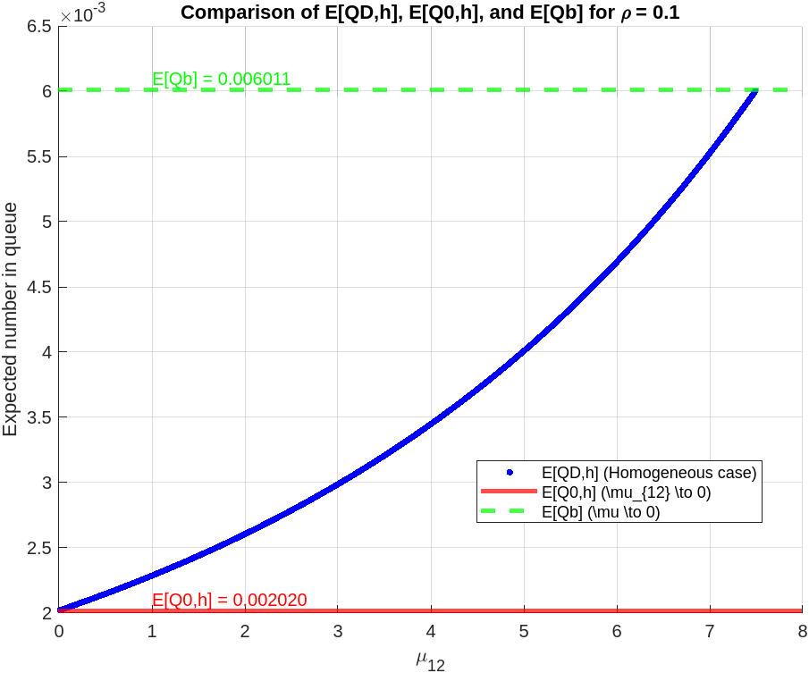
(a) $\rho=0.1$

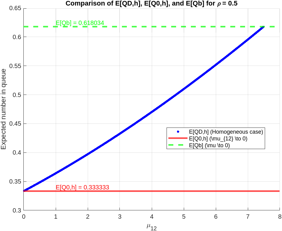
(b) $\rho=0.5$

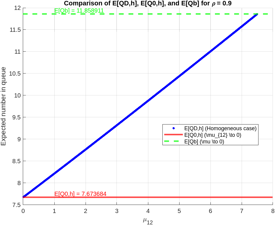
(c) $\rho=0.9$

Figure 1: Impact on the system performance by $\mu_{12}$ when $\mu_{1}=\mu_{2}=\mu$

It is evident that the dependence between service times has a significant impact on system performance. This impact becomes increasingly pronounced as $\mu$ goes to 0. For a small value of $\rho$ (say $\rho=0.1$), the increase in $E[Q_{D,h}]$ is initially slower than linear, specifically, it grows more slowly than the slope of the straight line connecting $(0,E[Q_{0,h}])$ and $(7.5,E[Q_{b}])$ as $\mu_{12}$ increases to a certain point. Beyond that point, the growth becomes faster than linear. As $\rho$ increases, the curve of $E[Q_{D,h}]$ approaches that of the straight line (see, for example, the curve for $\rho=0.9$). For $\rho=0.1$, 0.5, and 0.9, the maximum value of $E[Q_{D,h}]$ is approximately 2.9757, 1.8541, and 1.5454 times as large as $E[Q_{0,h}]$, respectively, for the model with independent servers. These results show that the relative impact of service time dependence decreases as $\rho$ increases—from 2.9757 to 1.5454 as $\rho$ increases from 0.1 to 0.9.

We conjecture that, in the homogeneous case, $E[Q_{D,h}]$ is an increasing function of $\mu_{12}$ for any fixed value of $\rho$.

5.5 Numerical analysis when $\mu_{1}\neq\mu_{2}$

For the heterogeneous case, where $\mu_{1}\neq\mu_{2}$, we must specify the ratio $\theta=\mu_{1}/\mu_{2}$, or equivalently $\mu_{1}=\theta\mu_{2}$, in order to produce a specific plot of $E[Q_{D}]$. For $\theta=1.5$, 2, and 3, Figures 2 – 4 show that the impact of correlated service times is similar to that in the homogeneous server case, as long as the ratio $\theta$ is not too large (e.g., for the three values of $\theta$ specified above).

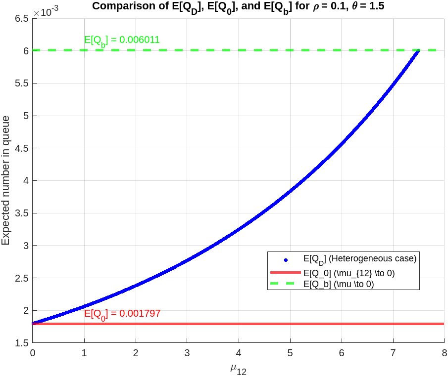
(a) $\rho=0.1$

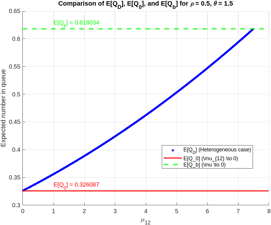
(b) $\rho=0.5$

(c) $\rho=0.9$

Figure 2: Impact on the system performance by $\mu_{12}$ when $\mu_{1}\neq\mu_{2}=\mu$ with $\theta=1.5$

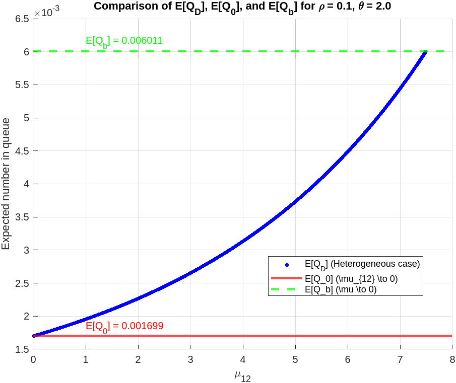
(a) $\rho=0.1$

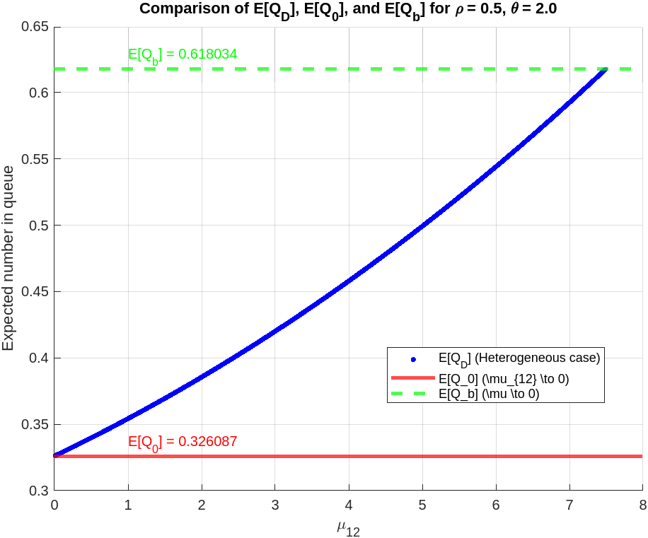
(b) $\rho=0.5$

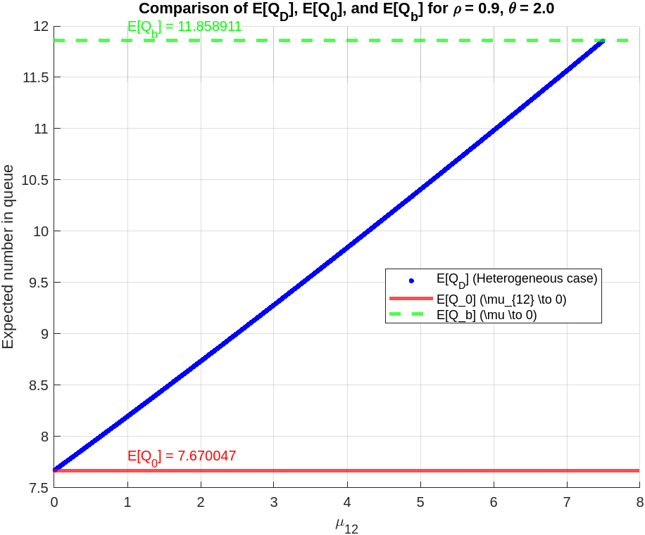
(c) $\rho=0.9$

Figure 3: Impact on the system performance by $\mu_{12}$ when $\mu_{1}\neq\mu_{2}=\mu$ with $\theta=2$

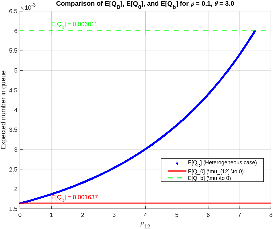
(a) $\rho=0.1$

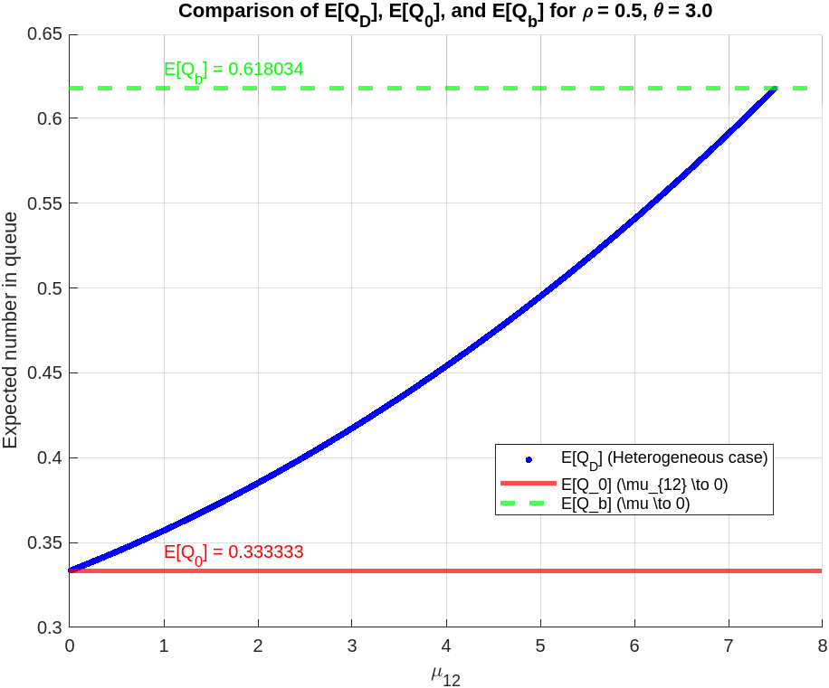
(b) $\rho=0.5$

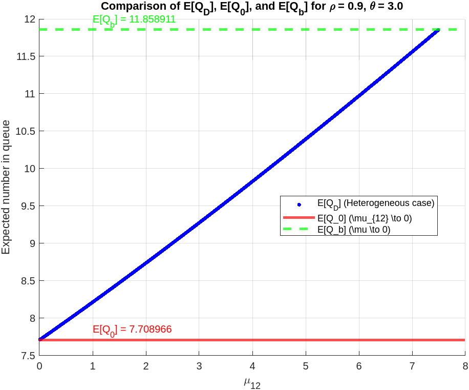
(c) $\rho=0.9$

Figure 4: Impact on the system performance by $\mu_{12}$ when $\mu_{1}\neq\mu_{2}=\mu$ with $\theta=3$

However, when the value of $\theta$ is very large — for example, $\theta=15$ in Figure 5 — the expected number $E[Q_{D}]$ in the dependent case can be smaller than that in the independent case when $\mu_{12}$ is relatively small. This effect becomes less noticeable as $\rho$ increases. When $\rho$ is sufficiently large, we no longer expect better performance from dependence; that is, $E[Q_{D}]$ remains greater than $E[Q_{0}]$ for all $\mu_{12}$. When $\rho$ is very large (e.g., $\rho=0.9$), the curve of $E[Q_{D}]$ becomes nearly linear with respect to $\mu_{12}$, even when $\theta$ is large. This is an interesting observation.

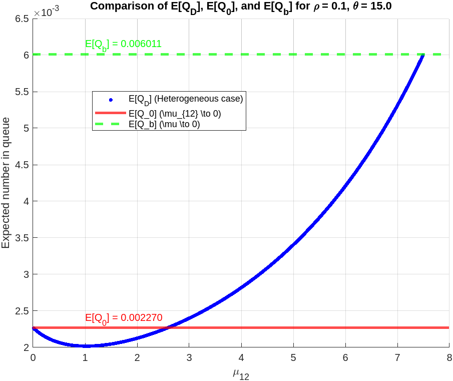
(a) $\rho=0.1$

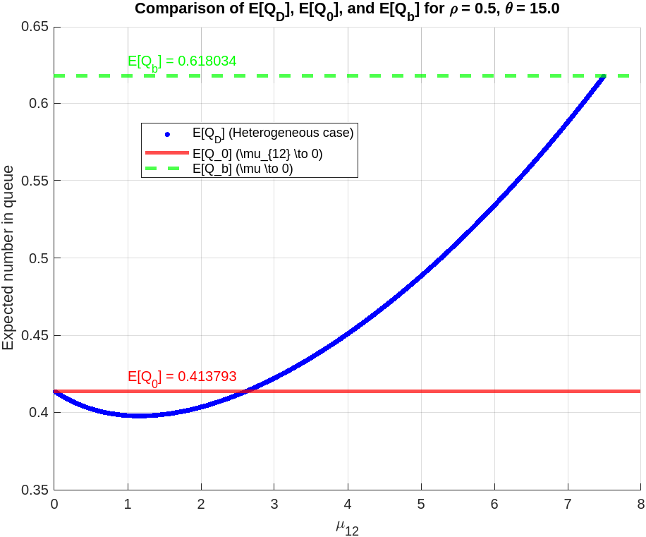
(b) $\rho=0.5$

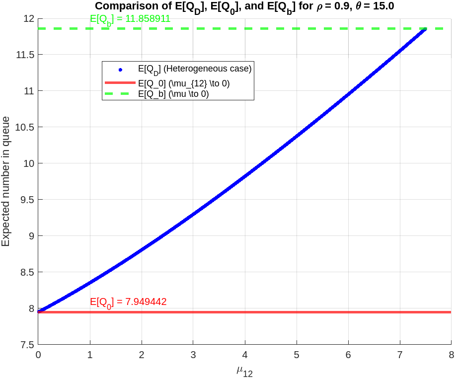
(c) $\rho=0.9$

Figure 5: Impact on the system performance by $\mu_{12}$ when $\mu_{1}\neq\mu_{2}=\mu$ with $\theta=15$

6 Concluding remarks

In this paper, we proposed a new approach that leads to a Markovian queueing model for systems with positively correlated servers. This approach successfully addresses the concerns raised by Mitchell et al. [19], who wrote:

“It is not clear that the birth–death equation approach can be modified to incorporate dependent service times. Moreover, any such formulation would very likely be analytically intractable.”

We have shown that the birth–death equation approach can indeed be extended to handle dependent service times. However, the resulting Markov chain for the queueing process is no longer a birth–death process due to singularities in the service time density. Nevertheless, for the $M/M_{D}/2$ model, the Markov chain remains analytically tractable.

We expect that this approach can be applied to other two-dimensional queueing systems with dependent servers, and can be also extended to systems of dimension higher than two.

References

- [1] Avi-Itzhak, B. and Levy, H. (2001) Bufferr equirement and server ordering in a tandem queue with correlated service times, Mathematics of Operations Research, 26(2), 358–74.
- [2] Boxma, O.J. (1979) On a tandem queueing model with identical service times at both counters, I Advances in applied probability, 11(3), 616–643.
- [3] Boxma, O.J. (1979) On a tandem queueing model with identical service times at both counters, II Advances in applied probability, 11(3), 644–659.
- [4] Boxma, O.J. and Deng, Q. (2000) Asymptotic behavior of the tandem queueing system with identical service times at both queues, Mathematical Methods of Operations Research, 52, 307–23.
- [5] Browning, S.G. (1998) Tandem queues with blocking: A comparison between dependent and independent service, Operations Research, 46(3), 424–429.
- [6] Calo, S.B. (1979) The message channel, a tandem interconnection of queues, Part I, IBM Report RC 6868.
- [7] Calo, S.B. (1980) The message channel, a tandem interconnection of queues, Part II, IBM Report RC 7170.
- [8] Conolly, B.W. and Choo, Q.H. (1979) The waiting time process for a generalized correlated queue with exponential demand and service, SIAM Journal on Applied Mathematics, 37(2), 263–275.
- [9] Erlang, A.K. (1909) The theory of probabilities and telephone conversations, Ny Tidsskrift for Matematik, B, 20, 33–39.
- [10] Hoon Choo, Q. and Conolly, B. (1980) Waiting time analysis for a tandem queue with correlated service, European journal of operational research, 4(5), 337–345.
- [11] Gumbel, H. (1960) Waiting lines with heterogeneous servers, Operations Research, 8, 504–511.
- [12] Kelly, F.P. (1976) Networks of queues, Adv. Appl. Prob., 8, 416–432.
- [13] Kelly, F.P. (1979) Reversibility and Stochastic Networks, Wiley, Chichester.
- [14] Kelly, F.P (1982) The throughput of a series of buffers, Adv. in Appl. Probab., 14, 633–653.
- [15] Kleinrock, L. (1964) Communication Nets: Stochastic Message Flow and Delay, McGraw-Hill, New York.
- [16] Kotz, S., Balakrishnan, N., and Johnson, N.L. (2000) Continuous Multivariate Distributions: Models and Applications, John Wiley & Sons.
- [17] Lin, G.D., Dou, X., and Kuriki, S. (2019) The bivariate lack-of-memory distributions, Sankhyā: The Indian Journal of Statistics, 81, 273–297.
- [18] Marshall, A.W. and Olkin, I. (1967) A multivariate exponential distribution, Journal of the American Statistical Association. 62, 30–44.
- [19] Mitchell, C.R., Paulson, A.S. and Beswick, C.A. (1977) The effect of correlated exponential service times on single server tandem queues, Naval Research Logistics Quarterly, 24(1), 95–112.
- [20] Pang, G. and Whitt, W. (2012) Infinite-server queues with batch arrivals and dependent service times, Probability in the Engineering and Informational Sciences, 26, 197–220.
- [21] Pang, G. and Whitt, W. (2012) The impact of dependent service times on large-scale service systems, Manufacturing and Service Operations Management, 14(2), 226–278.
- [22] Pang, G. and Whitt, W. (2013) Two-parameter heavy-traffic limits for infinite-server queues with dependent service times, Queueing Systems, 73(2), 119–146.
- [23] Pinedo, M. and Wolff, R.W. (1982) A comparison between tandem queues with dependent and independent service times, Operations Research, 30(3), 464–479.
- [24] Sandmann, W. (2007) Performance evaluation of dependent two-stage services, Proceedings of the 21st European Conference on Modelling and Simulation (ECMS), 74–9.
- [25] Sandmann, W. (2010) Delays in a series of queues: Independent versus identical service times, The IEEE symposium on Computers and Communications, 32–37.
- [26] Sandmann, W. (2012) Delays in a series of queues with correlated service times, Journal of Network and Computer Applications, 35(5), 1415–1423.
- [27] Singh, V.P. (1970) Two-server Markovian queues with balking: heterogeneous vs. homogeneous servers, Operations Research, 18, 145–159.
- [28] Wolff, R.W. (1982) Tandem queues with dependant service times in light traffic, Operations research, 30, 619–635.
- [29] Ziedins, I. (1993) Tandem queues with correlate service times and finite capacity, Math. O.R., 18, 901–915.