Weak transcription factor clustering at binding sites can facilitate information transfer from molecular signals

Abstract

Transcription factor concentrations provide signals to cells that allow them to regulate gene expression to make correct cell fate decisions. Calculations for noise bounds in gene regulation suggest that clustering or cooperative binding of transcription factors decreases signal-to-noise ratios at binding sites. However, clustering of transcription factor molecules around binding sites is frequently observed. We develop two complementary models for clustering transcription factors at binding site sensors that allow us to study information transfer from a signal to a variable relevant to development, namely future cell fates, on the example of the signal morphogen Bicoid in early fly development. We find that weak cooperativity or clustering can allow for maximal information transfer, especially about the relevant variable. Why clustering is beneficial for transfer depends on how long the binding site sensor measures the signal before affecting downstream gene expression: for short measurements, clustering allows for the implementation of a switch, while for long measurements, weak clustering allows the sensor to access maximal developmental information provided in a nonlinear signal. Finally, we find that clustering can facilitate binding site sensors to achieve an optimal bound to molecular sensing, the information bottleneck (IB) bound. This IB optimality appears consistent with a biologically intuitive optimization.

Cells differentiate and develop in response to chemical signals. These signals differentially regulate the expression of target genes, either directly or through a series of transcription factors. The canonical example from early fly development is the transcription factor Bicoid, an initially maternally supplied signal which regulates the development of cells along the head-to-tail body axis of the embryo. The gradient of Bicoid concentration along this embryonal axis encodes the information that cells need to develop into the correct body segments Nüsslein-Volhard and Wieschaus (1980); Driever and Nüsslein-Volhard (1988); Gregor et al. (2007a). Together with two other maternal signals, Bicoid regulates the expression of the downstream gap genes, which allows nuclei along the embryonal axes to develop into almost distinguishable cell fates, with a standard deviation of ca 0.1% of the embryonal length Gregor et al. (2007a); Dubuis et al. (2013).

Transcription factors like Bicoid regulate genes by binding to binding sites in the regulatory regions of the genome, including promoter or enhancer regions. Noise bounds for the sensing of transcription factor signals in early work on information transfer in gene regulation were inspired by the Berg-Purcell limit, a classical bound for sensing Berg and Purcell (1977); Bialek and Setayeshgar (2005); ten Wolde et al. (2016); Kaizu et al. (2014). Further work on these bounds to include cooperativity Bialek and Setayeshgar (2008), also in absence of diffusive noise Skoge et al. (2011, 2013), has shown that the signal-to-noise ratio at the binding site decreases when binding occurs cooperatively. These noise bound calculations suggest that cooperative binding and clustering at binding sites reduce the information flow in gene regulation and should therefore not be optimal from an information-theoretic perspective.

Yet, proteins involved in gene regulation do cluster, which raises a question about whether this can be consistent with efficient information transfer. Experimentally, clustering of proteins, including Bicoid, around binding sites has been observed Mir et al. (2017, 2018); Dufourt et al. (2018); Munshi et al. (2025); we use the phrase clustering here to remain agnostic of the precise mechanism that leads to a positive affinity between proteins McSwiggen et al. (2019), as local clusters can indeed occur from a variety of mechanisms. For example, transcription factors can bind cooperatively at binding sites Lebrecht et al. (2005), or cluster around the binding site region, potentially as a consequence of binding or biomolecular condensation Hyman et al. (2014); Shin and Brangwynne (2017); Hnisz et al. (2017); Sabari et al. (2018); McSwiggen et al. (2019); Hannon and Eisen (2024). Condensation phenomena are most relevant for high concentrations. Transcription factors are often expressed at low (nM) concentrations, in the case of Bicoid corresponding to 10000 molecules at the anterior (head) and 0-10 molecules at the posterior (tail) of the embryo Gregor et al. (2007a); Abu-Arish et al. (2010); Mir et al. (2017). Yet, also at lower concentrations, proteins can manifest clustering in the context of clusters around other highly-expressed proteins, or pre-wetted, local clusters only around binding sites Morin et al. (2022); Munshi et al. (2025); Mir et al. (2018); Dufourt et al. (2018). Bicoid itself has disordered or low-complexity domains, which are associated with clustering Kato and McKnight (2018), and indeed, hubs or clusters involving Bicoid have been observed Mir et al. (2017, 2018); Dufourt et al. (2018); Munshi et al. (2025). Therefore, we want to understand, in absence of a precise mechanism for clustering, how transcription factor clustering at binding sites affects the information transfer in gene regulation.

To address the question of information transfer, we go beyond sensing errors and signal-to-noise ratios Bialek and Setayeshgar (2008); Skoge et al. (2011); Malaguti and Ten Wolde (2021); Mora and Nemenman (2019), and study the information that the occupation at the binding site sensor encodes both about the signal as well as about possible downstream cell fates (section I). We study only a single binding site sensor and only the local environment around this sensor along the DNA, ignoring the three-dimensional microenvironment or potential competition effect between sensors. We model this sensor inspired by a regulatory region that regulates the expression of the main Bicoid target, hunchback. We focus on two types of models that have been used to study proteins that tend to co-localize due to a protein-protein affinity; we only study these proteins around binding sites. In section II, we work with a model established in the context of cooperative binding, where the occupation follows a Hill-function, to guide expectations. In section III, we develop a more mechanistic model of clustering molecules at and around a single sensor based on an Ising-like model Skoge et al. (2011); Morin et al. (2022); this model allows us to study how clustering beyond binding sites and therefore beyond cooperative interactions affects information transfer. Since it is difficult to estimate the relevant timescales during which occupation at binding sites leads to an regulatory impact, we study two limiting measurement times; we attempt to estimate a long measurement time that captures the maximum of what is biologically realistic.

We find that clustering improves information transfer for short measurement durations. For long measurement durations we find that clustering can reduce the information that the binding site can capture about the signal, in agreement with previous work. However, the information that is of developmental importance for the embryo is barely affected by clustering, up until clustering strengths equivalent to a Hill function coefficient of approximately three. This suggests that weak clustering may be beneficial for efficient transfer of regulatory information.

Finally, in section IV, we investigate whether realistic binding site sensors can achieve an abstract, data-driven bound for information transfer, the information bottleneck bound Tishby et al. (2000). We find that this is theoretically possible for a variety of binding site parameters, but that many randomly generated binding site configurations fall short of the bound.

I Information Flow through binding site sensors

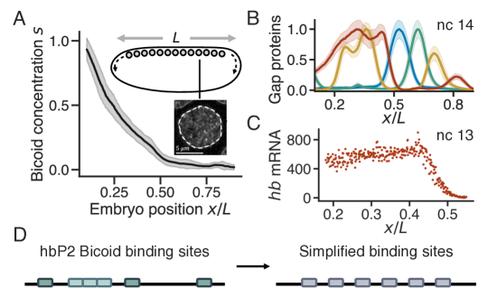
Figure 1: Signal processing in the fly embryo. A) The normalized maternal Bicoid gradient Gregor et al. (2007a) along the embryonal head-to-tail axis, which regulates the four gap genes; inset shows hetereogeneous Bicoid concentration inside a single nucleus (airy-scan image with experimental design described in Ref. Munshi et al. (2025)). B) The normalized concentration of the four gap gene proteins (hunchback, giant, Krüppel, knirps in red, yellow, blue, green respectively) in nc 14 as a function of embryonal position x, scaled to embryo length L, exemplifying the developing body segments. C) hb RNA expression in nc 13 as a function of embryonal position Little et al. (2013), when hb expression is mostly regulated through the proximal hbP2 enhancer region. D) Sketch of real the hbP2 region Park et al. (2019), containing ca. 6 binding sites, and our simplification with equidistant binding sites of equivalent binding strength.

The Bicoid morphogen gradient is one of a few regulatory signals that are required for correct body-part segmentation in the fly embryo (Fig. 1A) Driever and Nüsslein-Volhard (1988); Gregor et al. (2007a); Liu et al. (2013). The information provided in Bicoid is transferred downstream via the gap genes, whose expression begins consistently after twelve rounds of nuclear divisions, in nuclear cycle (nc) 13; just 10 mins later, these gap genes patterns are fully established (Fig. 1B) and provide enough information for nuclei along the embryonal axis to develop into distinguishable cell fates Dubuis et al. (2013). Although gap proteins act as transcription factors with mutually activating and repressive functions Jaeger (2011), in nc 13 the gap gene hunchback (hb) can be considered as being regulated predominantly by Bicoid. The expression of hb in nc 13 (Fig. 1C) is driven by the P2 (proximal) promoter or enhancer region (hbP2), which has frequently served as a test region for gene expression Tkacik et al. (2008); Ling et al. (2019); Park et al. (2019); Eck et al. (2020); Desponds et al. (2020). Here, we consider a simplified version of this enhancer to address the question of transcription factor clustering: we treat the approximately six binding sites as equi-distant binding sites with equal binding energies (Fig. 1D).

We assume that a regulatory region or binding site region with $h$ cooperative binding sites has access to the averaged fraction of occupied sites during a time interval $\tau$, denoted by variable $C=\frac{1}{\tau}\int_{0}^{\tau}c(t)dt$, with $c$ denoting the occupation at time $t$. This occupation $C$ corresponds to the nucleus’s measurement of the signal $s$. We consider downstream gene expression to be approximately proportional to $C$, consistent with simple models of gene regulation, in which $C$ can determine the number of polymerases recruited to the promoter.

To assess how much information about the external signal of concentration $s$ the regulatory region (or sensor) can capture, we use the mutual information

$$I(C;s)=\int ds\int dCP(C,s)\log_{2}\frac{P(C,s)}{P(C)P(s)}\textrm{,}$$ (1)

which depends on probability distribution $P(C|s)$, describing the nucleus’s measurement of $s$.

We use the Bicoid expression profile Gregor et al. (2007a) (Fig. 1A) to obtain the prior distribution of signalling molecules $P(s)$, by taking $P(s|x)$ Gaussian and $P(x)$ uniform. For stochastic models of binding at a binding site, we can obtain $P(C|s)$ from simulations (section III). For sufficiently long time intervals $\tau$, longer than the correlation time, the probability distribution $P(C|s)$ approaches a Gaussian distribution, i.e.,

$$P(C|s)=\frac{1}{\sqrt{2\pi\sigma_{C}(s)^{2}}}\exp\Big{[}-\frac{(C(s)-\bar{C}(s))^{2}}{2\sigma_{C}(s)^{2}}\Big{]}\textrm{,}$$ (2)

where $\sigma_{C}(s)^{2}$ is the variance and $\bar{C}$ the mean occupation that occurs during the interval $\tau$. For such long $\tau$, $\bar{C}$ corresponds to the mean occupation in steady state, $\bar{C}:=\langle C\rangle=\frac{1}{\tau}\int_{0}^{\tau}\langle c\rangle dt=\langle c\rangle$, where $\langle\ldots\rangle$ denotes the ensemble average. We can calculate $\sigma_{C}(s)^{2}$ and $\bar{C}$ for a specific stochastic process, and use this Gaussian approximation to assess information transfer through a specific binding site.

The information provided by the signal could be different from the information that the embryo needs to develop correctly. For example, a signal may provide more information than needed in specific instances. In the fly embryo, correct development requires that nuclei along the embryonal axis can develop into distinct fates, determined by their position Dubuis et al. (2013); Tkačik and Gregor (2021). We thus use the information that the regulatory region can convey about nuclear position $x$, $I(C;x)$ Dubuis et al. (2013); Bauer et al. (2021), as a variable of relevance to the embryo. We calculate $I(C;x)$ using Eq. 1 with $P(C|x)=\int P(C|s)P(s|x)ds$. We can therefore assess precision in the transfer of molecular signals through gene regulation with both the information captured about the signal, $I(C;s)$ as well as the information of relevance, $I(C,x)$, allowing for a more nuanced assessment than possible with signal-to-noise ratios.

II Simple model for gene regulation: weak cooperativity is optimal for multiple measurement times

In canonical models for gene regulation, the mean occupation of binding sites $\bar{C}$ for cooperative binding is described by a Hill function Hill (1910); Jong (2002); Weiss (1997); Bialek (2012); Tkacik and Walczak (2011); Marzen et al. (2013); Bauer (2022),

$$\bar{C}=\frac{s^{h}}{k+s^{h}}\textrm{.}$$ (3)

where $s$ is the normalized signal concentration, $k$ the dissociation equilibrium constant and $h$ the Hill coefficient corresponding to the number of binding sites or cooperatively binding molecules (Fig. 2A,B). Hill functions originate from a heuristic deterministic description that compares the average number of free and bound binding sites over long time intervals, and accurately describe gene expression outputs in population-averaged experiments. For single cells, gene expression and mean binding site occupations may be more complicated. Yet, Hill functions provide an interesting limiting case as they describe the steepest possible binding site occupation from a regulatory region with $h$ binding sites in single cells Martinez-Corral et al. (2024).

In this section, we study binding site sensors described by Hill functions. We calculate the probability with which a binding site sensor is occupied during a time interval given a particular signal, by assuming that this occupation is Gaussian distributed around a mean (Eq. 2). To calculate the variance, we first design a stochastic process for which the mean occupation can be represented with a Hill function.

We assume that binding only occurs when $h$ molecules bind at the same time to $h$ binding sites (Fig. 2A). The probability for the binding site to be occupied at time $t$, $P(c=0,t)$, can be described by a master equation for the two states of being occupied or not occupied, $c=1$ and $c=0$, $\frac{dP(c=0,t)}{dt}=k_{\textrm{off}}-(k_{\textrm{off}}+k_{\textrm{on}}s^{h})P(c=0,t)\textrm{,}$ where $k_{\textrm{on}}$ and $k_{\textrm{off}}$ are the rate constants for binding and unbinding. The equilibrium constant $k$ can be written as $k=k_{\textrm{off}}/k_{\textrm{on}}$. The mean occupation in steady state for this process corresponds indeed to a Hill function (Eq. 3), if we can assume that the time averaged mean normalized occupation that the binding site has access to, $\bar{C}$, corresponds to the ensemble averaged, steady-state mean, $\bar{C}=\langle c\rangle$.

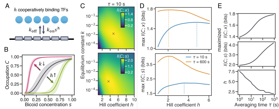
Figure 2: Information transfer through a sensor with cooperative binding sites. A) Sketch of cooperative binding of transcription factors (TFs) to six binding sites. B) Mean occupation according to the Hill function for different parameters $h$ and $k$. C) The information $I(C;x)$ (and $I(C;s)$) as a function of $h$ and $k$ shows a well-defined maximum (cross) in parameter space. We use $k_{\textrm{off}}=1/$s. D) The maximum possible information $I(C;x)$ and $I(C;s)$ over all values of $k$ for different $h$ (maxima indicated by vertical lines). For the longer measurement time $\tau=600$ s (orange), the maximal information value per $h$ is higher than for $\tau=10$ s (blue), and maximal values are reached for lower $h$. E) The optimized information $I(C;x)$ and $I(C;s)$ over all $k$ and $h$ as a function of measurement time $\tau$, with $I(C;x)$ reaching its maximal bound $I(s,x)$ at approximately $\tau\sim 1000s$. E bottom) The value of $h$ at the optimum of $I(C;x)$ decreases with measurement time $\tau$.

To obtain the distribution of variable $C$, we calculate the variance in occupation, $\sigma_{C}(s)^{2}=\langle(C-\bar{C})^{2}\rangle$. An estimate of this variance can be obtained from the observation that the regulatory region is either occupied or unoccupied during each measurement; in time $\tau$, there will be of order $N\approx\tau/\tau_{c}$ independent measurements, where the correlation time

$$\tau_{c}=\frac{1}{k_{\textrm{off}}+k_{\textrm{on}}s^{h}}$$ (4)

can be obtained from the master equation. Therefore, we expect a binomial variance of order $\sigma_{C}(s)^{2}\approx\frac{1}{N}\bar{C}(1-\bar{C})$, where in steady state $\bar{C}(1-\bar{C})$ corresponds to the instantaneous variance Kaizu et al. (2014); ten Wolde et al. (2016); Bialek (2012). We follow the calculation in Kaizu et al. (2014) to obtain the exact result (Appendix VI.1),

$$\sigma_{\bar{C}}(s)^{2}=\frac{2\tau_{c}}{\tau}\bar{C}(1-\bar{C})\textrm{,}$$ (5)

in agreement with Kaizu et al. (2014); ten Wolde et al. (2016); Bialek (2012). This differs from the ad-hoc expectation by a factor of two; this factor is required when the concentration $s$ is inferred from the occupation during the time interval $\tau$, whereas inferring the concentration from the discrete number of (independent) binding events allows for a lower variance Endres and Wingreen (2009).

The standard deviation in occupation (Eq. 5) increases with the correlation time of the occupation, which in turn increases with Hill coefficient $h$ (Eq. 4). Therefore, one might expect that cooperativity in the form of $h>1$ reduces the information transfer, consistent with Refs Bialek and Setayeshgar (2008); Skoge et al. (2011, 2013).

We can now calculate how precisely a binding site sensor can measure signal concentration $s$, provided the sensor is determined by parameters $h$ and $k$ and has access to a time-averaged occupation during a particular interval $\tau$. We calculate the distribution for the occupation $P(C|s)$ using Eqs. 3, 5 and 2. We investigate two representative measurement times for a short and long measurement $\tau$. The long measurement corresponds approximately to the duration of nc 13 (10 min), provided that transcription factor residence times of order $\approx 1$ s can set an effective timescale for $k_{\textrm{off}}\sim 1/\text{s}$. The short measurement is still longer than the correlation time, to ensure that the Gaussian approximation is valid; we chose a time of approximately $\tau=10$ s.

Both the information about the signal $I(C;s)$ as well as the information of relevance to the embryo, $I(C;x)$ show a clear maximum at a specific parameter combination of $h$ and $k$ per measurement time, similar to earlier work that also incorporated noise in RNA production Tkačik et al. (2009) (Fig. 2C for $\tau=10$ s, Appendix VI.1 for a more detailed discussion and $\tau=10$ min). For each value of cooperativity $h$, more information can maximally be captured over $k$ for longer $\tau$ (Fig. 2D) Even for the longer $\tau$, the optimal number of cooperative binding sites is larger than one, suggesting that on realistic timescales some cooperativity may be optimal.

We note that $I(C;x)$ saturates at approximately $1.8$ bits, as the binding site cannot extract more information about cell fates than the signal Bicoid itself provides (additional signals would allow for more information Dubuis et al. (2013)). For long $\tau$, a range of cooperativities $h$ achieves the optimum (exact optimum positions at $h\approx 2.1$ and $h\approx 4.8$). Even if we compare this measurement to one where $h$ binding sites are treated independently, the information could not be higher than $1.8$ bits.

Both $I(C;s)$ and $I(C;x)$ increase with $\tau$ when optimized over $h$ and $k$ (Fig. 2E). The optimal number of cooperatively binding molecules $h$, maximizing $I(C;x)$, decreases with measurement time (Fig. 2E bottom). For increasing $\tau\to\infty$, it saturates at values $h\approx 1.38$; and remains larger than two even at measurement times of $1000$ s.

From an information-theoretic perspective, it makes sense that steep thresholds or high $h$ are optimal for shorter measurement times, associated with high noise or variance in $P(C|s)$: binary, threshold-like measurements are known to provide the most information when noise is high Bauer et al. (2021); Mattingly et al. (2018). For longer $\tau$ and more precise measurements, we find that weak cooperativity is optimal or does not reduce information up until $h<3$. This has two reasons: first, $h=1$ does not lead to a linear $\bar{C}$, which makes intuition difficult. Second, for considering $I(C;x)$, we should note that the Bicoid gradient itself is not a linear input; we know from rate-distortion theory that an optimal map $\bar{C}$ that reads a variable $x$ that is conveyed through a signal with a non-linear mean ($\bar{s}(x)$) should itself be a nonlinear function of the signal (concretely $\bar{C}(s)=\bar{x}(s)$ Cover and Thomas (2012)). Since optimizing $I(C;x)$ is additionally convex, different non-linear maps can achieve the optimum.

If the longer measurement time of 10 minutes is biologically realistic for the fly embryo, an optimally adjusted binding site sensor would have approximately 2-3 cooperatively binding molecules. Interestingly, this does indeed correspond to the number of strongly binding Bcd molecules in the hbP2 enhancer Park et al. (2019). We do not expect an exact match, as our estimates for timescales are approximative, but are encouraged to find a reasonable estimate for $h$. We conclude that our heuristic Hill-function model suggests that some cooperativity is optimal, consistent with information-theoretical expectations considering the functional form of the signal. Yet, Hill-function model suffers from the significant shortcoming that we are forced to consider longer measurement times and cannot capture the binding and unbinding of individual molecules. To check the role of clustering in more detail, we next investigate the role of clustering of transcription factors around binding sites with a more realistic mechanistic model.

III Mechanistic model for clustering transcription factors

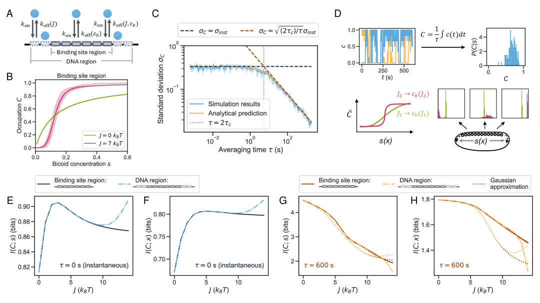
Figure 3: Information transfer through a binding site or DNA region with individual clustering signal molecules. A) Sketch of model binding sites (solid) and surrounding sites on DNA (dashed; DNA region), with on- and off-rates for transcription factors. B) Steady-state occupation $\bar{C}$ of the binding site region (no surrounding sites) for $J=0$ and $\varepsilon_{b}\approx 14.1$, and $J=7$ and $\varepsilon_{b}\approx 8.2$ as a function of signal concentration, $s$, with the standard deviation (shaded region) for measurement time $\tau=10$ min. C) Standard deviation $\sigma_{C}$ from simulations of the binding site region matches the analytical solution from the master equation (which can be approximated by Eq. 7 as shown in Appendix VI C, Fig 7A), decreasing from its instantaneous value to a $1/\sqrt{\tau}$-scaling for longer $\tau$. Simulations are for parameter values $\mu=-14.0$, $J=3.5$ and $\varepsilon_{b}\approx 11.1$, with error bars over 5 independent repeats of the calculation, each based on 20 simulations, D) Sketch of the simulation procedure: for all $\mu$ corresponding to signal concentrations $s(x)$ along the embryonal axis, we perform Gillespie simulations and average occupation over time $\tau$ to obtain $C$. For each $s$, we estimate $P(C|s)$ based on histograms of $C$ from 100 repeats of the simulation. We calculate $I(C;s)$ and $I(C;x)$ from this distribution for each $J$, using a modified parameter $\varepsilon_{b}$ to retain half maximum occupation at $x\sim 0.47$. E+F) Mutual information in an instantaneous measurement: Clustering improves both $I(C;x)$ and $I(C;s)$, with a maximum for clustering strength $J\approx 3$. For high $J$, the occupation of additional sites along the DNA can further increase the information. G+H) Mutual information in a long measurement ($\tau=600$ s): Clustering decreases $I(C;s)$. The information $I(C;x)$ also decreases with clustering, but with minor information loss (5% of the maximum) up until intermediate clustering strengths of $J=3$.

III.1 Clustering affects both occupation mean and variance

To find a more realistic description of the occupation of a binding site sensor that incorporates binding and unbinding of individual transcription factors, we adapt an Ising model for a small, one-dimensional region of the DNA around the binding sites (Fig. 3A) Skoge et al. (2011). We fix the concentration of the signal transcription factors with chemical potential $\mu$, parameterize the binding energy for a binding site with $\varepsilon_{b}$, and describe clustering between neighbouring transcription factors with clustering strength $J$. In short, we describe our system with the Hamiltonian

$$\hat{H}=-J\sum_{i=1}^{N-1}c_{i}c_{i+1}-\mu\sum_{i=1}^{N}c_{i}-\varepsilon_{b}\sum_{i=1}^{N^{\prime}}c_{i}\textrm{,}$$ (6)

where $c_{i}=\{0,1\}$ denotes occupation at site $i$ and $N$ ($N^{\prime}$) denotes the number of (binding) sites in the system. Transcription factors appear from and leave to a bath (the nucleus) with rates $k_{\textrm{on}}$ and $k_{\textrm{off}}$, consistent with detailed balance Glauber (1963). For an isolated site that is not a binding site, the rates satisfy $k_{\textrm{on}}/k_{\textrm{off,free}}=e^{-\beta\mu}$; we set $\beta=1$ and use $k_{\textrm{off,free}}$ to determine the timescale of the simulation (Appendix VI.2). As arrival statistics should not depend on the details of the site, we use the same $k_{\textrm{on}}$ for all sites, and incorporate the effect of binding to a binding site or clustering with a neighbouring transcription factor in the rate $k_{\textrm{off}}$, which thus varies for different configurations. We refer to $J$, $\mu$ and $\varepsilon_{b}$ in units of $k_{B}T$.

A core difference between cooperativity and clustering is that a clustered hub of proteins can extend beyond the binding site region. Thus, we study two types of binding site sensors: first, a binding site sensor with $N^{\prime}=N=6$ binding sites (Fig. 3A, binding site region), and second, an extended binding site sensor with $N^{\prime}=6$ binding sites surrounded by two sites on each side that represent the surrounding DNA region, such that $N=10$ (Fig. 3A, DNA region). We will see that an interesting effect of the DNA region sensor is that steeper thresholds are achievable for strong clustering strengths $J$, which can be beneficial for short measurement times.

We obtain the normalized time-averaged occupation $C$ of the binding site sensor (referred to as ‘occupation’ from now on) with a Gillespie algorithm Gillespie (1976, 1977). However, to guide expectations, we first explore the mean $\bar{C}$ and variance $\sigma_{C}^{2}$ of the occupation $C$ as a function of input parameters. We refer to Appendix VI.3 for the stochastic master equation and detailed calculations.

The mean occupation $\bar{C}(s)$ increases more steeply for higher clustering strength $J$ (Fig. 3B). Clustering also shifts the signal concentration $s$ at which the mean occupation of the binding site sensor reaches its half-maximal occupation; varying the binding energy can compensate for this shift (Fig. 3B). A Hill function can approximate the mean occupation, semi-validating our approach in the first section. The fitted Hill coefficients are $h\approx 1$ and $h\approx 4$ for $J=0$, $\varepsilon_{b}\approx 14.1$ and $J=7$, $\varepsilon_{b}\approx 8.2$, respectively.

The variance around the mean occupation $\bar{C}$ in steady state can be obtained using the correlation function (Appendix VI.3, cf. Eq. 5, following Ref. Skoge et al. (2011); Zhang and Berry (2005)). We find

$$\sigma_{C}^{2}\approx 2\sigma_{\textrm{inst}}^{2}\frac{e^{-\tau/\tau_{c}}+\frac{\tau}{\tau_{c}}-1}{(\tau/\tau_{c})^{2}}\textrm{,}$$ (7)

where $\sigma_{\textrm{inst}}^{2}$ is the instantaneous variance in steady state. This expression reduces to $\sigma_{C}(\tau)\approx\sigma_{\textrm{inst}}\text{ for }\tau<2\tau_{c}$ and to $\sigma_{C}(\tau)\approx\sqrt{\frac{2\tau_{c}}{\tau}}\sigma_{\textrm{inst}}\text{ for }\tau>2\tau_{c}$, as expected Kaizu et al. (2014). We validate this approximation by showing excellent agreement of the variance from Eq. 7 with a semi-analytical expression using the master equation (Appendix VI.3 Fig. 7A,B), which matches the stochastic simulations (Fig. 3C). Clustering increases the correlation time of a measurement, which in turn increases the variance (Appendix VI.3, Skoge et al. (2011)).

We thus conclude that the strength with which transcription factors cluster, $J$, affects both the mean and variance of the occupation at the binding site sensor. While stronger clustering leads to increased variance, the concomitant effect on the mean occupation may foil the conclusion that clustering always decreases information, just as in section II.

Before presenting how clustering affects information transfer in the fly embryo in this model, we explain one modification that we make to reduce the parameter space which we sample. We know that a larger clustering strength $J$ shifts the finite mean occupation toward anterior parts of the embryo. This behaviour is consistent with the idea that clustering increases the local concentration of transcription factors Hnisz et al. (2017); Trojanowski et al. (2022). Yet, as a consequence, many combinations of $J$ and the binding energy $\varepsilon_{b}$ lead to sensors that capture barely any information. Such sensors are not biologically realistic: If a particular clustering strength is set by properties of transcription factor proteins, and if the information transfer from Bicoid is important, the embryo would likely have faced evolutionary pressures that ensure that the binding energy is adjusted, through mutations in binding sequences, to make information transfer feasible. Therefore, as we vary $J$ in the following section, we choose to vary $\varepsilon_{b}$ at the same time, setting $\varepsilon_{b}$ such that the binding site sensor can produce half maximal expression at $x\approx 0.47$, as expected for hb expression in the fly embryo (Fig. 1C, Appendix VI.3 Fig. 7E). This reduces the parameter combinations we study. While we do not prove that this choice is information-theoretically optimal, we see in section IV that it is close to the information bottleneck bound.

III.2 In the fly embryo, weak clustering can lead to an increase in mutual information about cell-fates

To assess the information obtained by the binding site sensor, we again focus on measurement durations that represent a short and long measurement time. We estimate timescales relevant to the fly embryo (Appendix VI.2, Abu-Arish et al. (2010); Fernandes et al. (2022); Gregor et al. (2007b); Porcher et al. (2010)). We use an instantaneous measurement and a long timescale corresponding to 10 min as the two limiting cases for a measurement duration.

We obtain probability distributions and mutual informations from Gillespie simulations (Appendix VI.4) for values of chemical potential $\mu(x)$ that yield a particular $s$ (Fig. 3D). As probability distributions should approach the Gaussian distribution for long measurement times, we also calculate information using the Gaussian approximation with $\bar{C}$ and $\sigma_{C}$ from the previous section (Appendix VI.3, Eq. 18, Eq. 7) for comparison.

For instantaneous measurements, weak clustering increases information transfer: both $I(C;s)$ and $I(C;x)$ increase with $J$ with a local maximum at $J\approx 3$ (Fig. 3E,F). This is consistent with our results from Hill-function models, and the intuition that steeper, more thresholded measurements are optimal when the measurement is noisy. For stronger clustering strengths, the information reduces, as higher correlation times increase the measurement noise of a binding site region with such strong clustering.

For the DNA region sensor that includes a larger region around the binding site, stronger clustering of $J\approx 10$ improves information transfer again. This increase in information is related to the mean occupation: the effective Hill coefficient for the binding site region reaches $h=6$ from below for high $J$ (Appendix VI.3 Fig.7E), in agreement with the fact that the Hill coefficient that fits stochastic gene expression is bounded by the number of binding sites Estrada et al. (2016); Martinez-Corral et al. (2024); in contrast, the steepness for the DNA region can increase further, as clusters extend beyond just the binding sites.

The fact that clustering can lead to occupation of surrounding DNA sites could therefore be an avenue by which clustering can increase information transfer in the embryo (see also Refs. Rippe (2022); Pontius (1993)). However, such strong clustering is likely also associated with a source of error for signals expressed at low concentrations that our model does not capture: for small numbers of signal molecules and multiple binding site regions, large clusters around one region may deplete signal molecules from other binding site regions, and therefore contribute to a more noisy measurement in realistic settings. Since we do not take into account these depletion effects, we cannot evaluate this effect here.

For long measurement times, clustering reduces the precision with which the binding site sensor can measure the signal (Fig. 3G). Since for long $\tau$, measurements are more precise (low variance), a steeper mean activation of occupation is less beneficial. The information then suffers from an increase in variance, as the increase in correlation time caused by clustering implies that less independent measurements can be performed during interval $\tau$, consistent with earlier work Skoge et al. (2011). However, we note that the information of relevance to the embryo that the binding site sensor obtains, $I(C;x)$, plateaus and does not decrease significantly (within five percent) for weak clustering strengths up to $J\approx 3$ (Fig. 3H). This result implies that clustering corresponding to Hill coefficients up to $h\approx 3$ is indeed consistent with optimal information transfer, and therefore validates and refines our findings from section II.

The Gaussian approximation, which we used in section II, works well for long $\tau$, until medium clustering strengths, $J\approx 6$, above which $P(C|s)$ becomes too strongly peaked at empty or full occupation (Fig. 3G,H). Finally, we observe that the difference between the extended DNA sensor and binding site region is marginal for the long measurement time, as the information is not limited by the steepness of the mean occupation.

Together, our results show that weak clustering is not detrimental to signal processing at the binding sites in early fly development.

IV The information bottleneck bound is achievable with realistic binding site sensors

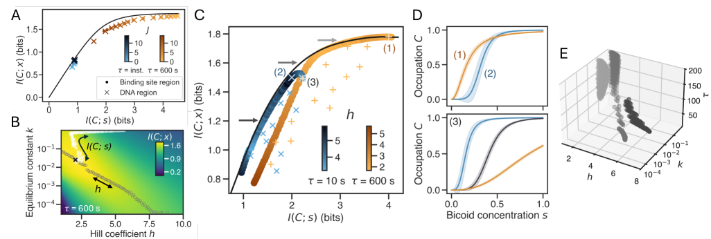
Figure 4: Binding site sensors that incorporate cooperativity and clustering can theoretically achieve the information bottleneck optimization goal. A) Sensors from the mechanistic model for instantaneous (blue) and long measurement times (orange) for changing clustering strength $J$ (color shade) on the information plane, with optimal IB bound from data in black. B) In the Hill function model, different binding site sensors parameterized by $h$ and $k$ are optimal for different constraints: the paths that mark a (variable) constraint on $h$ and a (variable) constraint on $I(C;s)$ (IB goal) are marked with grey circles and white crosses respectively. C) Information plane with IB bound in black and a selection of exemplary binding site sensors (blue crosses and orange plusses for $\tau=10$ s and $\tau=600$ s, respectively) show that randomly chosen binding sites are well below the bound. The sensors that optimize $I(C;x)$ for a given $I(C;s)$ in our parameter ranges of $h$ and $k$ are shown with larger circles; color shade indicates the value of $h$. D) Selected binding site sensors (1,2) from panel C representing the sensors along the IB bound (top), and sensors that represent point (3) in panel C (bottom, for $\tau=10$ s in blue, $60$ s in grey and $600$ s in orange). E) Optimal values of $h$, $k$ and $\tau$ for binding site sensors fitted to $P(C|s)$ from IB optimization, for three values on the bound in Fig. 1C (grey arrows) show that a variety of binding site sensors are consistent with the IB bound.

In the previous sections, we discussed $I(C;x)$, as well as the information that the binding site can capture about the signal, $I(C;s)$ as variables that quantify information flow, and assumed that functional binding sites should optimize these quantities. We discussed constraints, such as a constraint on the number of binding sites through Hill coefficient $h$, or a constraint on the binding energy as clustering increases. In this section, we describe binding site sensors that are optimized for an optimization goal called the information bottleneck, corresponding to optimizing $I(C;x)$ with a constraint on $I(C;s)$.

The information transfer from a molecular signal via a binding site region to downstream gene expression can be viewed as an information bottleneck (IB) problem Tishby et al. (2000): the binding site sensor $C$ presents a bottleneck between a signal $s$ and a variable of importance to the embryo, the position along the embryonal axis $x$, describing possible cell fates downstream Bauer et al. (2021); Bauer and Bialek (2023). The distribution $P(C|s)$ can be optimized such that that $I(C;x)$ is maximal for different values of $I(C;s)$, corresponding to the optimization goal Tishby et al. (2000):

$$\underset{P(C|s)}{\textrm{max}}\quad I(C;x)-\lambda I(C;s)\textrm{.}$$ (8)

The value of the Lagrangian multiplier $\lambda$ fixes the binding site capacity $I(C;s)$ to a specific value during optimization. For each value of $\lambda$ and therefore for each value of $I(C;s)$ we can find the optimal binding site sensor and the information $I(C;x)$ it can convey (Appendix VI.5). This optimal bound or optimal sensor distribution $P(C|s)$ is obtained directly from the input data, described by the distribution that maps relevant variable to the signal $P(s|x)$. The optimal bound of maximal $I(C;x)$ for each $I(C;s)$ divides the information plane (Fig. 4 A,C) into an allowed region on or below the optimal IB bound and a forbidden region above.

The quantity constrained in the IB problem is $I(C;s)$, which is determined by physical parameters describing the binding site sensor, including, e.g., the number of binding sites, clustering $J$ or binding energy $\varepsilon_{b}$, as well as diffusive timescales or the local environment of the binding site. In absence of knowing which of these parameters are constrained, a constraint on $I(C;s)$ can serve as a reasonable, general constraint. The IB bound dictates the tradeoff between $I(C;s)$ and $I(C;x)$, where an ideal sensor measures with the smallest possible $I(C;s)$ for the largest possible $I(C;x)$. The IB bound has recently been explored in the context of molecular sensing, and has predicted several features of enhancer networks that appear in the fly embryo as optimal, such as a need for multiple enhancers or a combination of binding sites for different signals Bauer et al. (2021).

We compare realistic binding site sensors to this bound by showing pairs of $I(C;s)$ and $I(C;x)$ from binding site sensors with specific parameter combinations and models on the information plane. We begin with binding site sensors from the mechanistic simulations, for both measurement times and varying $J$ (Fig. 4A). Strikingly, all binding site sensors are close to the information bound, for all values of $J$. Sensors with longer measurements $\tau$ measure more precisely and occupy regions higher in the information plane than sensors with instantaneous measurements, which also cover a smaller region of phase space (orange vs blue in Fig. 4A).

Since we do not know what $I(C;s)$ is physically possible and therefore what specific value point or range of values in the information plane is reasonable, we take sensors close to the IB bound as consistent with IB optimality, while sensors that are not optimal would appear far below the bound. Some binding site sensors are within $10\%$ of the maximally achievable $I(C;x)$ (light orange), at higher $I(C;s)$; these are the sensors with weak clustering, up to weak clustering values of $J\sim 3$. In Fig. 4A, we see that the IB bound for Bicoid is such that an abstract IB-optimal sensor can within 20% of the bound of 1.8 bits when sensing with a capacity of 1.8 bits (elbow of IB plot). The sensors with $J\sim 3-5$ are close to the elbow of the plot. Together, we find that weak clustering is beneficial also from an IB perspective, since sensors with finite $J$ are close to the entire IB bound, especially the plateau and elbow.

It may be surprising that all binding site sensors from the mechanistic model for all values of clustering $J$ are close to the IB bound. Our choice of constraining $\varepsilon_{b}$ for each $J$ to fix the half-maximal occupation to the middle of the embryo thus implicitly presents an effective optimization consistent with the information bottleneck. While variation of $\varepsilon_{b}$ may have allowed us to push even closer to the bound, it is interesting that our biologically motivated choice satisfies the bound well, as it suggests that the IB bound may be consistent with biologically motivated intuition.

To explore more binding site sensors, we return to the Hill-function models from section II. First, we visualize the effect of changing the constraint from fixed $h$ to fixed $I(C;s)$ (Fig. 4B). The optimal sensor parameters differ for different constraints, intersecting at the optimum. The effect of the IB constraint on Hill coefficient $h$ is subtle: for decreasing $I(C;s)$, $h$ initially increases, followed by a decrease until equilibrium constant $k$ is so large that the occupation of an individual binding site sensor barely reaches 50% for the highest $s$ (Appendix VI.5). This suggests that forcing sensors for a single measurement time to occupy all parts of the IB plot is not biologically sensible. Therefore, we do not consider binding site sensors with maximal occupations below 0.5. Nevertheless, screening a variety of $h$ and $k$ allows us to investigate information transmission for sensors that are abstractly possible.

Binding site sensors with varying $h$ and $k$ can fall on a wide region below the IB bound (symbols in Fig. 4C), for both $\tau$. Sensors that measure longer achieve more information, especially for more optimized sensors (orange crosses extending to higher $I(C;x)$). To investigate whether some binding site sensors match the IB bound, we numerically select the binding site sensor that maximizes $I(C;x)$ for each $I(C;s)$ (as in 4B), and show the corresponding information pairs in the information plane (blue and orange lines, with color shade indicating $h$, Fig. 4C). The optimal sensors are on the IB bound for different regions of phase space: the sensors that measure for longer $\tau$ no longer achieve the IB bound for low $I(C;s)$, due to our constraint on a sensor’s mean occupation. Nevertheless, the sensors for short $\tau$ achieve the bound for low $I(C;s)$. Overall, we find that it is indeed possible to achieve the abstract and data-driven IB bound with these realistic sensors.

Encouraged by the fact that binding site models can yield sensors on the IB bound, we study the features of these sensors in more detail. In principle, we observe the occupation mean of optimal sensors becomes less steep for higher $I(C;s)$ (Fig 4D top). However, we only show two exemplary sensors for two points on the bound here, and additional sensors may be IB-optimal may be more subtle if we consider additional $\tau$. We know that the IB problem is highly convex: different sensors can yield the same $I(C;s)$ and $I(C;x)$ and therefore end up at the same region of the information plane (Fig. 4D bottom). If we consider also additional measurement times, we find that multiple parameter combinations $h$, $k$ and $\tau$ yield sensors with the same $I(C;s)$ and $I(C;x)$ along the bound (Fig. 4E). This shows that multiple implementations of sensors can be consistent with information-theoretic optimization goals Bauer et al. (2025); nevertheless, randomly selected sensors are not optimal.

V Discussion and Conclusion

We developed two models that allow us to calculate the precision with which binding site sensors measure transcription factor signals, and the information about cell fates that the binding site can retain from the signal. Our first model based on Hill-functions relies on a series of approximations, including measurement times longer than correlation times, and does not describe the binding of individual molecules. To go beyond this, we developed a second more mechanistic model that also allows us to study clustering around a binding site region. We chose the occupation of a binding site region as the variable that needs to convey information downstream, for which a decrease in the signal-to-noise ratio due to clustering had previously been predicted. In both models, the presence of cooperativity or clustering can increase the information that the binding site region can convey for short measurements, and even for longer measurements, clustering does not significantly reduce this information. Our results are not sensitive to the details of signal transfer at the binding site: we verified that weak clustering is even more beneficial for a binding site region that induces hb expression not proportionally to its average occupation, but only when it is fully occupied Desponds et al. (2020) (Appendix VI.6 Fig. 8).

We also showed that binding site regions with clustering transcription factors are able to achieve information optimality as predicted by the information bottleneck bound. Since this bound can help us understand the regulatory architecture of the fly embryo Bauer et al. (2021), it is important to identify models for binding site regions that can achieve it. Here, we show that several binding site sensors would be consistent with this bound. We also found that biologically intuitive constraints, such as adjusting the binding energy to ensure that the binding site occupation changes most in the middle of the embryo, are consistent with the IB constraint. Therefore, it will be interesting to investigate further which realistic constraints on parameters, including molecule numbers or energy constraints Sokolowski et al. (2025); Tjalma et al. (2023); Tjalma and Wolde (2024); Nicoletti and Busiello (2024), are consistent with each other and with IB optimality.

The reason why clustering can be beneficial even when signals convey information is different depending on the duration of the time interval during which the sensor measures: For short measurement times, weak clustering improves precision as thresholded measurements are optimal for noisy sensing, and for long measurement times, weak clustering can lead to a nonlinear activation function that optimizes information flow towards a variable of importance, if its map with the signal is also nonlinear.

Our result that clustering can be beneficial for information transfer connects with current work on the importance of clustering around binding site regions in the context of transcription: clustering can buffer signal fluctuations, which improves accuracy for a constant signal that fluctuates Klosin et al. (2020); Deviri and Safran (2021). Here, we work towards understanding how clustering affects the processing of signals whose concentration conveys information. Our findings provide an information-theoretical understanding of the usefulness of clusters that stretch between and around binding sites Rippe (2022); Pontius (1993), and of the importance of weak interactions in the context of transcription Gao et al. (2018).

Our work has caveats. First, our parameter estimates to compare to the fly embryos are estimates, despite our efforts. Second, we did not incorporate diffusive noise in this work; diffusive noise or multiple instances of phase-separated droplets Cho et al. (2018) will change the correlation time for an individual measurement, and therefore the timescales in our system. Yet, that weak clustering is beneficial or that information bounds are reachable with realistic sensors should still apply, as the many realistic measurement times should lie in between the timescales we studied here. Third, we studied the simple problem of information transfer from a single signal through a single binding site, while in reality, multiple maternal signals provide information for multiple outputs, among them the four gap genes. The problem of joint information transfer could yield different optimal solutions; if these optimal solutions involve ‘modular’ encodings (about e.g. different parts of the embryo) that rely on steep thresholds, clustering at binding sites would become even more important. Relatedly, studying multiple binding site regions would be an important extension of our work: Since clustering, especially in the context of biomolecular condensation, would occur at multiple binding sites for different genes, competition effects between these binding sites could reduce the accuracy of information transfer. This loss of information could be avoided if signal-carrying transcription factors associate to clusters of other molecules, or if cluster shapes and sizes reliably capture the signal Mittag and Pappu (2022); Mir et al. (2018); Munshi et al. (2025). These are interesting directions for future work.

Acknowledgements. We are grateful to Ned Wingreen, Eric Wieschaus and William Bialek for many helpful discussions of questions, models and calculations relevant to this project. We thank Thomas Gregor and Mikhail Tikhonov for providing data for hb mRNA for Fig. 1C, and Rahul Munshi for providing an image of Bcd in Fig. 1A. We thank Riccardo Rao, Linda Dierikx, Max Metlitski, Caroline Holmes, Michal Levo, Thomas Gregor and his lab, Trudi Schüpbach and members of the Bauer group for comments and discussions. We acknowledge funding from the NWO Vidi Talent programme (NWO/VI.Vidi.223.169, MB), the NWO Science-XL grant OCENW.XL21.XL21.115 (AK and MB), and a TUDelft Start-up grant (JZ). A part of this work was performed at the Aspen Center for Physics, which is supported by National Science Foundation grant PHY-2210452.

VI Appendix

VI.1 Effective Hill function model: Variance and numerics

For the Hill function model, we assume that binding only occurs when $h$ molecules bind at the same time to $h$ binding sites. The chemical master equation for the two states of occupation at the binding site, $c=0$ and $c=1$, reads

$$\frac{dP(c=0,t)}{dt} =k_{\textrm{off}}-(k_{\textrm{off}}+k_{\textrm{on}}s^{h})P(c=0,t)\textrm{,}$$ (9)

where $k_{\textrm{on}}$ and $k_{\textrm{off}}$ are the rate constants for binding and unbinding. We assume that the signal concentration $s$ is not affected by binding, since the number of binding sites is typically much less than the number of signal molecules in the nucleus. We can solve the master equation,

$$P(c=0, t)=\frac{k_{\textrm{off}}}{k_{\textrm{off}}+k_{\textrm{on}}s^{h}}+$$

$$\left(P(c=0,t=0)-\frac{k_{\textrm{off}}}{k_{\textrm{off}}+k_{\textrm{on}}s^{h}}\right)e^{-(k_{\textrm{off}}+k_{\textrm{on}}s^{h})t}\textrm{,}$$

to find the mean at steady state. This mean indeed corresponds to the Hill function,

$$\bar{C}=\langle c\rangle=\frac{s^{h}}{k+s^{h}}\textrm{,}$$ (10)

as in the main text. Although the effective ergodic, long $\tau$ approximation that we need for the first equality ($\bar{C}=\langle c\rangle$) may not hold for single nuclei and shorter timescales, we proceed with this approach, as Hill-functions are established in gene regulation, and present an interesting and accurate limit for the true stochastic process, as described in the main text.

To calculate the variance, we consider the temporal correlation function at stationarity: $\kappa(\delta t)=\langle(C(0)-\bar{C})(C(\delta t)-\bar{C})\rangle$. This correlation function depends only on the time difference $\delta t$ Gardiner (2021). This allows us to write for the variance

$$\sigma_{C}(s)^{2} =\langle(C-\bar{C})^{2}\rangle\textrm{,}$$

$$=\frac{1}{(\tau)^{2}}\int_{0}^{\tau}\int_{0}^{\tau}\langle(C(t_{1})-\bar{C})(C(t_{2})-\bar{C})\rangle dt_{1}dt_{2}\textrm{,}$$

$$=\frac{1}{(\tau)^{2}}\int_{0}^{\tau}\int_{-t_{1}}^{\tau-t_{1}}\kappa(t)dtdt_{1}\textrm{,}$$ (11)

following the calculation in Ref. Kaizu et al. (2014). We swap the order of integration in Eq. VI.1 and exploit symmetry of $C(t)$ to perform the integration over $dt_{1}$:

$$\langle(C-\bar{C})^{2}\rangle =\frac{2}{\tau^{2}}\int_{0}^{\tau}dt\kappa(t)(\tau-t)\textrm{.}$$ (12)

This can be approximated further if the correlation function $\kappa(t)$ decays on a timescale shorter than the measurement time $\tau_{c}\ll\tau$,

$$\sigma_{C}(s)^{2}= \langle(C-\bar{C})^{2}\rangle\approx\frac{2}{\tau}\int_{0}^{\tau}dt\kappa(t)\textrm{.}$$

We can obtain $\kappa(t)$ from the solution from the master equation, Eq. 9,

$$\kappa(t)=\bar{C}(1-\bar{C})e^{-t/\tau_{c}}=k_{\rm off}k_{\rm on}s^{h}\tau_{c}^{2}e^{-t/\tau_{c}}$$ (13)

where $\tau_{c}$ is the correlation time from Eq. 4, and $\bar{C}(1-\bar{C})$ is the instantaneous variance as in the main text. Using $k=\frac{k_{\textrm{off}}}{k_{\rm on}}$, the variance can be expressed as

$$\sigma_{C}(s)^{2} =\frac{2}{\tau k_{\rm on}}\frac{ks^{h}}{(k+s^{h})^{3}}\textrm{,}$$

$$=\frac{2}{\tau k_{\rm off}}\frac{k^{2}s^{h}}{(k+s^{h})^{3}}\textrm{,}$$ (14)

$$=\frac{2\tau_{c}}{\tau}\bar{C}(1-\bar{C})\textrm{,}$$

for large $\tau$.

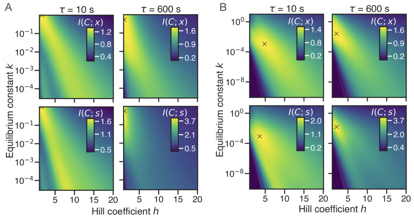
Figure 5: $I(C;x)$ and $I(C;s)$ as a function of $h$ and $k$ for two representative measurement times. A) $I(C;x)$ and $I(C;s)$ for $k_{\rm on}=10$ s^-1 nM^-h constant and varying $k_{\rm off}$; the maxima (cross) are always at the boundaries of parameterization space. B) Longer measurements with $\tau=600$ s show a similar behaviour to $\tau=10$ s, with a single optimum (cross). The left panels are replotted from the main with an increased range of $k$ values.

We use Eq. VI.1 to calculate the variance for our binding site sensors depending on parameters $k=k_{\rm off}/k_{\rm on}$, $h$ and $\tau$. The system depends on three free parameters, which can equivalently be chosen as $\tau k_{\rm on}$, $k_{\rm off}$ and $h$, or as $\tau k_{\rm off}$, $k_{\rm on}$ and $h$ (see Eq. VI.1). We opt for the second choice, as the first options errs towards a fallacy where the information can always increase as $k_{\rm off}$ increases (Fig. 5A with the maximum at the boundary of our range for $k$): in our system, the information to the binding site is provided only through the binding, and therefore a fast unbinding rate (and instantaneous disappearing of the molecule in our diffusive-free system) allows for more independent measurements. We therefore make the practical choice to keep $k_{\rm off}=1$ fixed and vary $k_{\rm on}$.

For comparison, Fig. 5B shows the information provided through a binding site with varying $h$ and $k$ (for constant $k_{\textrm{off}}$, as in the main text) for both measurement times side-by-side. The maximum information, indicated by a cross, occurs for finite $h$ and $k$.

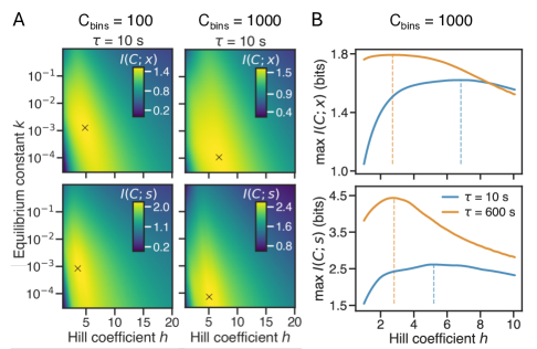
Figure 6: $I(C;x)$ and $I(C;s)$ using a changed number of bins for the numerical calculation of $P(C|s)$. A) The information $I(C;x)$ and $I(C;s)$ as a function of $h$ and $k$ for $\tau=10$ s shows maximum for binding site parameters (cross) at finite $h$, independent of numerical details. These details can affect the exact parameterization of the optimum, especially the dissociation equilibrium constant $k$. B) The maximum possible information $I(C;x)$ and $I(C;s)$ over all values of $k$ for different $h$. Finite $h$ is optimal for information transfer and the $h$ at the optimal mutual information $I(C;x)$ decreases with $\tau$, as in the main manuscript (Fig 2D).

We calculate probability distributions using the Gaussian assumption numerically, with 100 bins in the variable $C$ in the main text. To ensure that the finite number of bins does not affect our result, we recalculated the information as a function of binding site parameters $h$ and $k$ for a different numerical parameterization, with 1000 discrete bins for the variable $C$. We observe minor shifts for the parameters $h$ and $k$ that make up the maximum (Fig. 6), but the results do not change otherwise; therefore, we decided to use 100 bins for the main text.

We use 160 positions between 0.1 and 0.9 embryo length (for details see VI.4 for information about x-position bins).

VI.2 Time and length scales for the mechanistic model

The shortest distance between the centers of two Bicoid binding sites in the hb enhancer is 12 bp or approximately $4$ nm Fernandes et al. (2022). We thus use a grid cell of 4 nm. With this grid size, the concentrations used in our simulations are all below $10^{-12}$ molecules/grid cell, and thus satisfy the condition that the occupation at each binding site is much less than 1.

We assume that on the surrounding sites in the DNA region the transcription factors do not interact with DNA. Therefore, the off-rate in the absence of binding and clustering depends only the timescale in which a transcription factor diffuses away. To simplify the calculations, we rescale time such that $k_{\textrm{off,free}}$ is equal to 1 per time unit. One time unit is then equal to the mean time it takes a transcription factor to diffuse through the grid cell. We roughly estimate this timescale using the equation for the mean squared displacement (MSD) of a diffusing particle:

$$\textrm{MSD}=2KDt\to t=d_{x}^{2}/(2KD)$$ (15)

where $D$ is the diffusion constant, $d_{x}$ is the grid cell size and $K$ is the number of dimensions in which the transcription factor can leave the grid, with $K=3-1$ for a one dimensional grid. Values for the diffusion constant of Bicoid in literature range form 0.3$\mu m^{2}/s$ Gregor et al. (2007b) to 7.7$\mu m^{2}/s$ Porcher et al. (2010). We use the more likely and recent value of $D\approx 7\mu m^{2}/s$ as found by Abu-Arish et al. (2010). With these values we obtain a time unit of t=$1/k_{\textrm{off,free}}\approx 5.7\times 10^{-7}$ seconds, or $k_{\textrm{off,free}}=1.8\times 10^{6}/s$.

VI.3 Semi-analytical calculation of standard deviation for the mechanistic model

In the absence of clustering, $N$ states with different discrete occupations $n$ are enough to describe a system with $N$ sites. For a system with $N=6$ binding sites, the probability of the state with $n$ transcription factors bound at a timepoint $t$, $P_{n}(t)$ is given by

$$\dfrac{dP_{n}(t)}{dt} =[(N-(n-1))k_{\textrm{on}}]P_{n-1}(t)+[(n+1)k_{\textrm{off}}]P_{n+1}(t)$$

$$-[(N-n)k_{on}+nk_{\textrm{off}}]P_{n}(t),\quad\textrm{for}\quad 0<n<N,$$

$$\dfrac{dP_{0}(t)}{dt} =k_{\textrm{off}}P_{1}(t)-Nk_{\textrm{on}}P_{0}(t),$$

$$\dfrac{dP_{N}(t)}{dt} =k_{\textrm{on}}P_{N-1}(t)-Nk_{\textrm{off}}P_{N}(t),$$ (16)

where $P_{0}$ and $P_{N}$ describe probabilities for empty and full states. The variable $n$ is related to $c$ in the main manuscript by a normalization constant, i.e. $c=n/N$. Probabilities need to satisfy the constraint $\sum_{n=0}^{N}P_{n}(t)=1$. In the limit of a single binding site, we recover Eq. 9 with $h=1$ and, using $\mu=k_{B}T\ln s$, the steady state mean corresponding to the Hill function (Eq. 3 in the main manuscript, i.e. $\frac{s}{s+e^{-\beta\varepsilon_{b}}}$).

To incorporate clustering, we need to take into account all possible states of occupation in what could be seen as a graph-theoretical approach Wong and Gunawardena (2020): different states with the same occupation are connected with different rates. Taking into account all states requires a $2^{N}\times 2^{N}$ transition matrix with elements $M_{ij}$, where $i$ and $j$ run over all $2^{N}$ different states, described by their occupation for each binding site $\{n_{1},\ldots,n_{N}\}$, where each $n_{i}\in\{0,1\}$. For example, at a particular time, a binding site sensor might be in state $\{1,1,1,0,0,0\}$. We denote the occupation of each such state by $\tilde{c}_{i}=\sum_{k=1}^{N}(\{n_{k}\})/N$, so that $\tilde{c}$ is also a $2^{N}$ vector.

The probability to occupy state $i$, $\tilde{P_{i}}$, can be obtained from the solution of the master equation, via

$$\tilde{P_{i}}(t)=\sum_{j=1}^{2^{N}}\Big{(}e^{Mt}\Big{)}_{ij}\tilde{P_{j}}(0)\textrm{,}$$ (17)

where $\tilde{P_{j}}(0)$ denotes the initial probability of state $j$, which we take to be the steady state probability. The transition matrix $M$ has one zero eigenvalue, corresponding to steady state. Since all transition matrices at thermodynamic equilibrium can be transformed into a symmetric transition matrix $\tilde{W}$ with the same eigenvalues Zhang and Berry (2005), we know that this matrix is diagonalisable and will continue below with the representation using orthonormal eigenvectors, following references Skoge et al. (2011); Zhang and Berry (2005).

With the eigenvalues of $M$, $\lambda_{k}$, we can write $\dfrac{1}{\tau}\int_{0}^{\tau}e^{Mt}dt=\dfrac{1}{\tau}UAU^{-1}$, where $A$ is a diagonal matrix, the $k$ diagonal elements of which correspond to the integrals $\int_{0}^{\tau}e^{\lambda_{k}t}dt$ over all eigenvalues of $M$ and where $U$ is the matrix of eigenvectors of $M$. Since the first eigenvalue is zero, corresponding to the steady state eigenvalue, we obtain $A_{11}=\tau$ and $A_{ii}=\frac{1}{\lambda_{i}}(e^{\lambda_{i}\tau}-1)$ for $i>1$. This allows us to find the expectation value of the time-averaged occupation $C$,

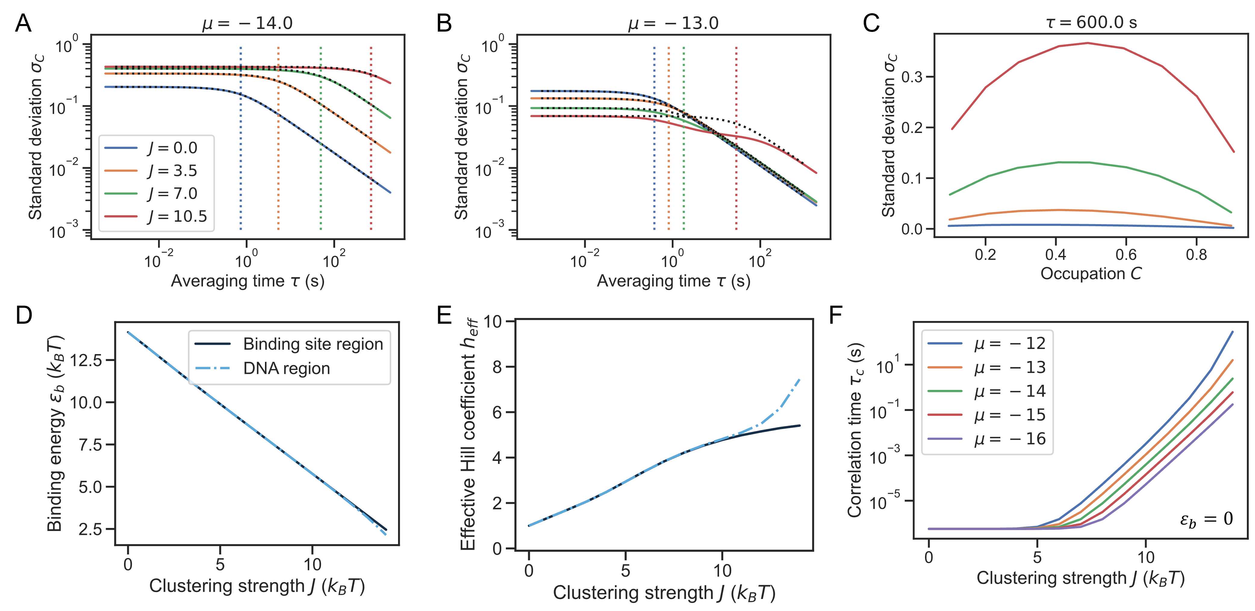
Figure 7: Mean and standard deviation of the mechanistic model from the master equation and analytic approximations. A+B) Comparison of standard deviation from diagonalization of Eq. 17 and Eq. 23 a value chemical potential $\mu$ corresponding to the anterior of the embryo, for different $J$; vertical bars indicate $2\tau_{c}$. We note that we shifted the value of $\varepsilon_{b}$ for these simulations, as shown in panel $D$. C) Standard deviation as a function of occupation $\bar{C}$ shows characteristic $\bar{C}(1-\bar{C})$ shape and increases with clustering strength. D) The binding energy $\varepsilon_{b}$ that guarantees half occupation at position $x\approx 0.47$ decreases almost linearly as a function of clustering strength $J$. E) Hill function fits to the mean occupation $\bar{C}$ show that the effective Hill coefficient $h$ approaches the 6 binding sites from below but can exceed this number for and extended sensor with 10 sites. F) The correlation time increases with clustering strengths throughout different values of chemical potential along the embryo.

$$\bar{C}(\tau)=\dfrac{1}{\tau}\sum_{i=1}^{2^{N}}\tilde{c}_{i}\left(\sum_{k=1}^{2^{N}}U_{ik}A_{kk}\sum_{j=1}^{2^{N}}(U^{-1})_{kj}\tilde{P_{j}}(0)\right)\textrm{.}$$ (18)

For small systems of $N=10$ and $N=6$ sites, Eq. 18 can be solved semi-analytically: we can obtain an exact analytic expression that is too complicated to write down. We plot this solution for the mean occupation from this semi-analytic treatment in Fig. 3B in our main manuscript. We note that the mean occupations for two different $J$ in Fig. 3B are calculated with a different value for $\varepsilon_{b}$, so that the occupation mean for higher $J$ shows its half occupation at $x=0.47$. We choose the value of $\varepsilon_{b}$ such that this is the case for every $J$ (Fig. 7D). Fitting Hill functions to the means obtained with Eq. 18 for these parameter combinations shows that for increasing $J$ the fitted Hill coefficient approaches the number of binding sites from below ($h\to N=6$) for the binding site region (see Fig. 7E); for the extended DNA sensor, we see that for high clustering strengths, higher Hill coefficients can be achieved.

We calculate the variance using Eq. 12. As for the mean, we can obtain a semi-analytic solution by solving the master equation, analogously to Eq. 18. Reference Skoge et al. (2011) obtained an analytic expression for the variance for the system with $N=6$ binding sites under periodic boundary conditions. We show the agreement of this limit and the semi-analytic solution for the variance from our master equation treatment in Fig. 7A,B, and discuss in the next paragraphs how to obtain this limit for our system.

We follow Refs Skoge et al. (2011) and Zhang and Berry (2005), noting that a symmetric transition matrix, $\tilde{W}$, which shares eigenvalues with $M$, can be obtained from $M$ via

$$\tilde{W}_{ij}=(\tilde{P}_{j}(0)/\tilde{P}_{i}(0))^{1/2}M_{ij}\textrm{,}$$ (19)

where $\tilde{P}_{i}(0)$ corresponds to the probability of state $i$ at equilibrium. The eigenvectors $\tilde{v}^{(k)}$ of $\tilde{W}$ are orthonormal, and can be related to the eigenvectors $v^{(k)}$ of $M$: $v_{i}^{(k)}=\sqrt{\tilde{P}_{i}(0)}\tilde{v}_{i}^{(k)}$Zhang and Berry (2005). This implies that the elements of $U^{-1}$ can be expressed in terms of the elements of $U$ via $(U^{-1})_{ki}\tilde{P}_{i}(0)=U_{ik}$. With that, the probabilities $\tilde{P}_{i}(t)$ can be fully expressed in terms of the eigenvectors and eigenvalues of $M$. Using $\delta\tilde{c}=\tilde{c}-\langle\tilde{c}\rangle$ to denote deviations from the occupation at steady state, we can then write the variance starting from Eq. 12

$$\sigma_{C}^{2} =\frac{2}{\tau^{2}}\int_{0}^{\tau}dt\kappa(t)(\tau-t)\textrm{,}$$

$$=\frac{2}{\tau^{2}}\int_{0}^{\tau}dt\sum_{i=1}^{2^{N}}\delta\tilde{c}_{i}\left(\sum_{k=1}^{2^{N}}v^{(k)}_{i}e^{\lambda_{k}t}\sum_{j=1}^{2^{N}}v^{(k)}_{j}\delta\tilde{c}_{j}\right)(\tau-t)\textrm{,}$$

$$=\frac{2}{\tau^{2}}\sum_{k=1}^{2^{N}}\Big{(}\sum_{i=1}^{2^{N}}\delta\tilde{c}_{i}v^{(k)}_{i}\Big{)}\Big{(}\sum_{j=1}^{2^{N}}\delta\tilde{c}_{j}v^{(k)}_{j}\Big{)}\int_{0}^{\tau}dte^{\lambda_{k}t}(\tau-t)\textrm{,}$$

$$=2\sum_{k=2}^{2^{N}}\Big{(}\sum_{i=1}^{2^{N}}\delta\tilde{c}_{i}v^{(k)}_{i}\Big{)}^{2}\Big{(}\frac{e^{\lambda_{k}\tau}-\lambda_{k}\tau-1}{\tau^{2}\lambda_{k}^{2}}\Big{)}\textrm{,}$$ (20)

where the terms $\sum_{i=1}^{2^{N}}\delta\tilde{c}_{i}v^{(k)}_{i}$ correspond to a projection of the fluctuations in occupation along the $k$th eigenvector and the sum in the last line starts with the second eigenvector, as $\sum_{i=1}^{2^{N}}\delta\tilde{c}_{i}v^{(0)}_{i}=0$. Finally, the instantaneous variance at equilibrium corresponds to the correlation function $\kappa(0)$ and can be expressed as

$$\sigma_{\textrm{inst}}^{2}=\sum_{k=2}^{2^{N}}\Big{(}\sum_{i=1}^{2^{N}}\delta\tilde{c}_{i}v^{(k)}_{i}\Big{)}^{2}\textrm{.}$$ (21)

While in principle all eigenvalues contribute to the sum, for long averaging times, we can only consider the contribution from the largest negative eigenvalue. Similarly, while the correlation time

$$\tau_{c}=\frac{1}{\sigma_{\textrm{inst}}^{2}}\int_{0}^{\infty}\kappa(t)dt$$ (22)

in principle involves multiple timescales, for many parameter values it is a valid approximation to consider only the largest of the non-zero (negative) eigenvalues, meaning that $\tau_{c}\approx 1/\lambda_{2}$. Therefore, following Ref Skoge et al. (2011), we find that

$$\sigma_{C}^{2}\approx\sigma_{\textrm{inst}}^{2}\mathcal{T}(\tau/\tau_{c})\textrm{,}$$ (23)

with

$$\mathcal{T}(x)=2\frac{e^{-x}+x-1}{x^{2}}\textrm{.}$$ (24)

We show the match of this expression to our semi-analytical calculation from master equation in Fig. 7A,B, as a function of measurement time $\tau$ for different $J$ and for a constant value of $\mu$. The variance follows the expected behaviour from Eq. 23 for all $J$, with a clear switch from the instantaneous variance to the scale where it decays as approximately $1/\sqrt{\tau}$ at approximately $\tau\approx 2\tau_{c}$. We show the match of this semi-analytical calculation and simulations in the main manuscript, for a single value of $\mu$.

In Fig. 7C, we show the variance for several values of $J$ across different mean occupations $\bar{C}$, which illustrates clearly the increase of the variance with $J$, due to the increase in the correlation time $\tau_{c}$ with $J$, in agreement with Skoge et al. (2011).

Finally, we show the correlation time from Eq. 22 from the numerical diagonalization of the master equation for different values of chemical potential as a function of clustering strength $J$ in 7F. In agreement with previous calculations, the correlation time increases with clustering strength.

VI.4 Concentration and occupation sampling for estimating $P(C|s)$ using the mechanistic model

We model presence and absence of transcription factors with 1 and 0s to avoid symmetry between the presence and absence of transcription factors.

To estimate the conditional probabilties $P(C|s)$ from simulations of the mechanistic model for clustering transcription factors, both the Bicoid concentration and the occupation must be discretized. To this end, we divide the concentration and occupation ranges into bins, and represent each bin using the value from the center of that bin.

The range of mean Bicoid concentrations (0-147nM) obtained from experimental data (Fig. 1A) was divided into 60 bins. Five additional bins were added, covering higher concentrations, to capture the fluctuations around the maximum mean concentration, resulting in a total of 65 bins covering a range of concentrations from 0-159nM. This number of bins was chosen such that the mutual information between the position and concentration differed by less than 0.01 from it’s limit as the number of bis goes to infinity (as estimated by the mutual information obtained with $10^{5}$ bins). The analytical calculations were repeated with a higher concentration sampling using ten times as many bins, to confirm that the choice of concentration sampling does not affect our conclusions (data not shown).

The number of occupation bins chosen for the histogram used to estimate $P(C|s)$ (Fig. 3D) influences the results obtained for the mutual information. When the number of bins is too low, the true distribution will not be accurately represented by the histogram, but if the number of bins is too high, the discrete nature of the simulations results will lead to artifacts in the final distribution. For this reason it is important to choose the right number of bins.

To this end, we compared the mutual information obtained using the histogram with that obtained using the Gaussian approximation for different numbers of bins. Since the Gaussian approximation is continuous, the mutual information results obtained using this approximation will converge to the true values as the number of bins increases. By comparing this to the mutual information calculated using the histogram, we can distinguish changes resulting from the mutual information converging to the true value from artifacts caused by the discrete nature of the simulation results.

Using this method we chose to use 400 bins for the histogram. For the Gaussian approximation, which does not suffer from the same type of artifacts we used 1000 bins. In the case of all-or-nothing expression described in Appendix VI.6 100 bins were used.

To obtain a value of signal concentration $s$ from the chemical potential $\mu$, we calculate the average concentration on a free, non-binding site. This sets the values of chemical potential that we use along the embryonal axis, $x$, allowing us to simulate the binding site sensor essentially in a grand-canonical ensemble. We use 160 positions between 0.1 and 0.9 embryo length. At each position $x$, the distribution of concentrations is assumed to be Gaussian; the mean concentration at each $x$ is found by assuming that the maximum mean concentration $s=1$ corresponds to 147 nM Abu-Arish et al. (2010).

VI.5 IB Optimization

We find the optimal information bound following Tishby et al. (2000): we iteratively optimize $P(C|s)$ from a random starting distribution, using

$$P(C|s)=\frac{P(C)}{Z(s,\lambda)}\exp\left[-\frac{1}{\lambda}\int dxP(x|s)\ln\left(\frac{P(x|s)}{P(x|C)}\right)\right],$$ (25)

where $Z$ is a normalization constant that ensures that $\int P(C|s)dC=1$. For each value of the Lagrangian multiplier $\lambda$, we iterate until $P(C|s)$ converges; from this optimal $P(C|s)$ we can then calculate a particular point along the bound in the information plane. The optimal $P(C|s)$ is thus determined from the data distribution $P(s,x)$, without any physical or mechanistic constraints on $P(C|s)$. $I(C;s)$ and $I(C;x)$ can be calculated from the optimal $P(C|s)$. Practically, we perform a discrete sum instead of an integral. We also used an approximate expression for the information bound Bauer and Bialek (2023), in which both $I(C;x)$ and $I(C;s)$ can be expressed using only a changing Lagrangian multiplier $\lambda$ and $I(s;x)$ (not shown). While it captures the bound approximately, it is slightly below the optimal bound and therefore also slightly below some binding site sensors, making it confusing for the purpose of this manuscript.

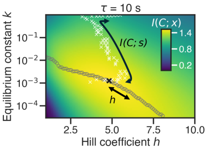
Figure 8: The information $I(C;x)$ as a function of binding site parameters $h$ and $k$ with symbols marking trajectories for a given constraint, for shorter $\tau=10$ s compared to the main manuscript Fig 4B. If $h$ are constrained to varying values of $h$, the optimal $I(C;x)$ lies along the circles, with lower $k$ for higher $h$. If $I(C;s)$ is constrained, the optimal $I(C;x)$ is marked with white crosses. The path of white crossed begins beyond the optimum (see blue line in Fig. 4C, which decreases as $I(C;s)$ is pushed beyond 2 bits). The maximum $I(C;x)$ is marked with a black cross.

To find the binding site sensors that also lie on the optimal bound, we search our sensors numerically: we first find all sensors with a particular $I(C;s)$ and then choose the sensor with the highest $I(C;x)$. This yields the white crosses in Fig. 4B and Fig. 8 (for $\tau=600$ s and $\tau=10$ s, respectively). In Fig. 8 we see the white path begin at smaller $h$ than the optimum, which corresponds to the part of the optimal bound in Fig 4C where $I(C;x)$ decreases for $I(C;s)>2$. As $I(C;x)$ decreases from its largest possible value, the path in the binding site parameter plane moves away from the optimum, towards larger values of $k$ and towards the boundary of the parameters we sample. When $I(C;s)$ just decreases away from the maximum, $h$ increases, but then decreases as the $I(C;s)$ decreases further. Eventually, the path arrives at the maximal value for $k$ we consider; if we increase $k$ further, the path continues along its current trajectory. However, in this case the binding site sensors along the optimal bound yield mean occupations that no longer include full occupation of the binding site at high $s$. Since we believe that such binding sites are no longer sensible, we typically only consider binding sites with a maximal normalized occupation $\bar{C}=0.6$; if we do so, the path continues towards significantly higher $h$ for almost constant $k$. This behaviour is again in principle consistent with the idea that lower $I(C;s)$ implies higher $h$, though we do note that we have effectively imposed an additional constraint on the binding site occupation; without this constraint, $h$ would continue to decrease slightly and $k$ would increase significantly, which implies an unphysically small $k_{\textrm{on}}$.

We hope to show with this trajectory in Figs. 4B and 8 that the constraints imposed matter significantly for finding the optimal binding site parameters.

VI.6 All-or-nothing expression

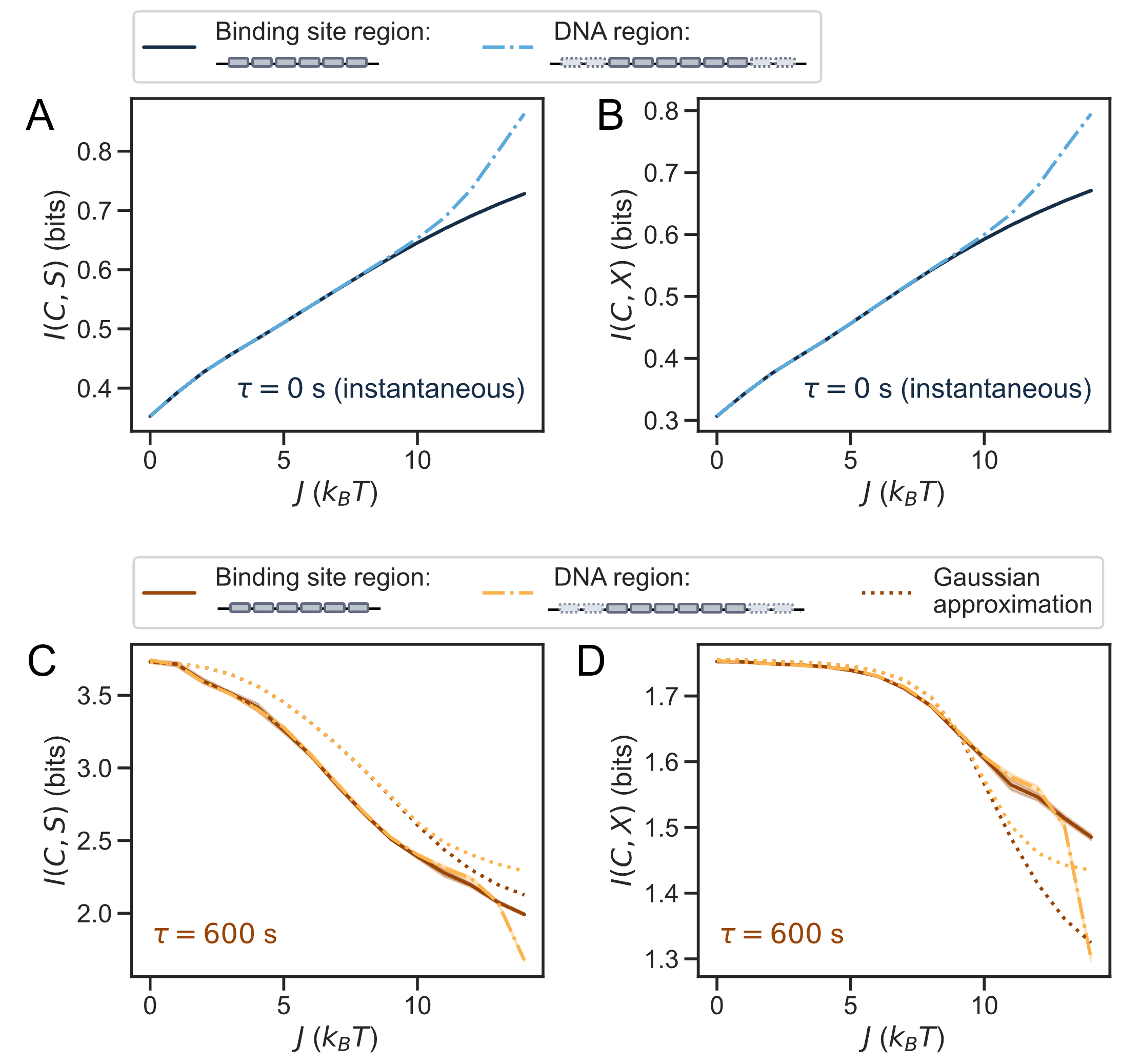
Figure 9: Mutual information for a transcription factor measurement which is processed in ’all-or-nothing’ fashion, i.e., where occupation is read out only in terms of two states: one state corresponding to a fully occupied binding site, that can activate gene expression downstream, and another state representing all other occupation states.

We assumed for almost all of the manuscript that gene expression regulated by the binding site sensor is proportional to the averaged occupation at the sensor. This seems biologically relevant, as polymerases could be recruited proportional to this average occupation, though of course this recruitment would add further noise into the process. Nevertheless, recent work on the hbP2 enhancer also discusses a scenario where gene expression (or polymerase recruitment) can only occur when the binding site is fully occupied Desponds et al. (2020).

We study this scenario numerically. We analyse our simulated trajectories for the long measurement time and instantaneous measurement, to obtain mean and variance for such a measurement $C^{\prime}$. These can be used to calculate probability distributions $P(C^{\prime}|s)$ as before. The mutual information $I(C^{\prime},s)$ and $I(C^{\prime},x)$ is shown in Fig. 9. For all measurements, the values of information are slightly lower than for the measurement that reads out the time-averaged occupation, since the all-or-nothing readout presents a course-graining that reduces information, consistent with the data-processing inequality. For the instantaneous measurement, clustering increases both relevant information quantities for all clustering strengths studied here; for the longer measurement, both informations decrease, with a strong plateau for $I(C^{\prime},x)$ for weak clustering strengths as in the main manuscript. Therefore, we conclude that our result that weak clustering is information-theoretically acceptable applies also to this different readout protocol.

References

- Nüsslein-Volhard and Wieschaus (1980) C. Nüsslein-Volhard and E. Wieschaus, Nature 287, 795 (1980).
- Driever and Nüsslein-Volhard (1988) W. Driever and C. Nüsslein-Volhard, Cell 54, 83 (1988).
- Gregor et al. (2007a) T. Gregor, D. W. Tank, E. F. Wieschaus, and W. Bialek, Cell 130, 153 (2007a).
- Dubuis et al. (2013) J. O. Dubuis, G. Tkačik, E. F. Wieschaus, T. Gregor, and W. Bialek, Proc Natl Acad Sci 110, 16301 (2013).
- Berg and Purcell (1977) H. C. Berg and E. M. Purcell, Biophys J 20, 193 (1977).
- Bialek and Setayeshgar (2005) W. Bialek and S. Setayeshgar, Proc Natl Acad Sci (USA) 102, 10040 (2005).
- ten Wolde et al. (2016) P. R. ten Wolde, N. B. Becker, T. E. Ouldridge, and A. Mugler, J. Stat. Mech. 162, 1395 (2016).
- Kaizu et al. (2014) K. Kaizu, W. H. de Ronde, J. Paijmans, K. Takahashi, F. Tostevin, and P. R. ten Wolde, Biophys J 106, 976 (2014).
- Bialek and Setayeshgar (2008) W. Bialek and S. Setayeshgar, Phys. Rev. Lett. 100, 258101 (2008).
- Skoge et al. (2011) M. Skoge, Y. Meir, and N. S. Wingreen, Phys. Rev. Lett. 107, 178101 (2011).
- Skoge et al. (2013) M. Skoge, S. Naqvi, Y. Meir, and N. S. Wingreen, Phys. Rev. Lett. 110, 248102 (2013).
- Mir et al. (2017) M. Mir, A. Reimer, J. E. Haines, X.-Y. Li, M. Stadler, H. Garcia, M. B. Eisen, and X. Darzacq, Genes Dev 31, 1784 (2017).
- Mir et al. (2018) M. Mir, M. R. Stadler, S. A. Ortiz, C. E. Hannon, M. M. Harrison, X. Darzacq, and M. B. Eisen, eLife 7, e40497 (2018).
- Dufourt et al. (2018) J. Dufourt, A. Trullo, J. Hunter, C. Fernandez, J. Lazaro, M. Dejean, L. Morales, S. Nait-Amer, K. N. Schulz, M. M. Harrison, C. Favard, O. Radulescu, and M. Lagha, Nature Communications 9, 5194 (2018).
- Munshi et al. (2025) R. Munshi, J. Ling, S. Ryabichko, E. F. Wieschaus, and T. Gregor, Science Advances 11, eadp3251 (2025).
- McSwiggen et al. (2019) D. T. McSwiggen, M. Mir, X. Darzacq, and R. Tjian, Genes Dev 33, 1619 (2019).
- Lebrecht et al. (2005) D. Lebrecht, M. Foehr, E. Smith, F. J. P. Lopes, C. E. Vanario-Alonso, J. Reinitz, D. S. Burz, and S. D. Hanes, Proceedings of the National Academy of Sciences 102, 13176 (2005), https://www.pnas.org/doi/pdf/10.1073/pnas.0506462102 .
- Hyman et al. (2014) A. A. Hyman, C. A. Weber, and F. Jülicher, Annu Rev Cell Dev Biol 30, 39 (2014).
- Shin and Brangwynne (2017) Y. Shin and C. P. Brangwynne, Science 357 (2017), 10.1126/science.aaf4382.
- Hnisz et al. (2017) D. Hnisz, K. Shrinivas, R. A. Young, A. K. Chakraborty, and P. A. Sharp, Cell 169, 13 (2017).
- Sabari et al. (2018) B. R. Sabari, A. Dall’Agnese, A. Boija, I. A. Klein, E. L. Coffey, K. Shrinivas, B. J. Abraham, N. M. Hannett, A. V. Zamudio, J. C. Manteiga, C. H. Li, Y. E. Guo, D. S. Day, J. Schuijers, E. Vasile, S. Malik, D. Hnisz, T. I. Lee, I. I. Cisse, R. G. Roeder, P. A. Sharp, A. K. Chakraborty, and R. A. Young, Science 361, eaar3958 (2018).
- Hannon and Eisen (2024) C. E. Hannon and M. B. Eisen, Elife 12, RP88221 (2024).
- Abu-Arish et al. (2010) A. Abu-Arish, A. Porcher, A. Czerwonka, N. Dostatni, and C. Fradin, Biophys J 99 (2010).
- Morin et al. (2022) J. A. Morin, S. Wittmann, S. Choubey, A. Klosin, S. Golfier, A. A. Hyman, F. Jülicher, and S. W. Grill, Nature Physics 18, 271 (2022).
- Kato and McKnight (2018) M. Kato and S. L. McKnight, Annual review of biochemistry 87, 351 (2018).
- Malaguti and Ten Wolde (2021) G. Malaguti and P. R. Ten Wolde, Elife 10, e62574 (2021).
- Mora and Nemenman (2019) T. Mora and I. Nemenman, Phys. Rev. Lett. 123, 198101 (2019).
- Tishby et al. (2000) N. Tishby, F. C. Pereira, and W. Bialek, in Proceedings of the 37th Annual Allerton Conference on Communication (Control and Computing, B Hajek and RS Sreenivas, eds, pp 368–377 (University of Illinois, 1999), 2000) arXiv:physics/0004057 .
- Little et al. (2013) S. C. Little, M. Tikhonov, and T. Gregor, Cell 154, 789 (2013).
- Park et al. (2019) J. Park, J. Estrada, G. Johnson, B. J. Vincent, C. Ricci-Tam, M. D. Bragdon, Y. Shulgina, A. Cha, Z. Wunderlich, J. Gunawardena, and A. H. DePace, Elife 8 (2019), 10.7554/eLife.41266.
- Liu et al. (2013) F. Liu, A. H. Morrison, and T. Gregor, Proc Natl Acad Sci (USA) 110, 6724 (2013).
- Jaeger (2011) J. Jaeger, Cellular and Molecular Life Sciences 68, 243 (2011).
- Tkacik et al. (2008) G. Tkacik, J. Callan, C. G., and W. Bialek, Proc Natl Acad Sci U S A 105, 12265 (2008).
- Ling et al. (2019) J. Ling, T. S. K. Y. Umezawa, and S. Small, Mol. Cell. 75, 1178 (2019).
- Eck et al. (2020) E. Eck, J. Liu, M. Kazemzadeh-Atoufi, S. Ghoreishi, S. A. Blythe, and H. G. Garcia, Elife 9, e56429 (2020).
- Desponds et al. (2020) J. Desponds, M. Vergassola, and A. M. Walczak, Elife 9, e49758 (2020).
- Tkačik and Gregor (2021) G. Tkačik and T. Gregor, Development 148, dev176065 (2021).
- Bauer et al. (2021) M. Bauer, M. Petkova, T. Gregor, E. F. Wieschaus, and W. Bialek, Proc. Natl. Acad. Sci. (USA) 118, e2109011118 (2021).
- Hill (1910) A. V. Hill, J. Physiol. 40, iv (1910).
- Jong (2002) H. D. Jong, J. Comput. Biol. 9, 67 (2002).
- Weiss (1997) J. N. Weiss, The FASEB Journal 11, 835 (1997).
- Bialek (2012) W. Bialek, Biophysics: Searching for Principles (Princeton University Press, 2012).
- Tkacik and Walczak (2011) G. Tkacik and A. Walczak, J. Phys.: Condens. Matter 23, 15310 (2011).
- Marzen et al. (2013) S. Marzen, H. G. Garcia, and R. Phillips, Journal of Molecular Biology 425, 1433 (2013), allosteric Interactions and Biological Regulation (Part I).
- Bauer (2022) M. Bauer, Biochem Soc Trans 50, 1365 (2022).
- Martinez-Corral et al. (2024) R. Martinez-Corral, K.-M. Nam, A. H. DePace, and J. Gunawardena, Proceedings of the National Academy of Sciences 121, e2318329121 (2024).
- Endres and Wingreen (2009) R. G. Endres and N. S. Wingreen, Phys. Rev. Lett. 103, 158101 (2009).
- Tkačik et al. (2009) G. Tkačik, A. M. Walczak, and W. Bialek, Phys. Rev. E—Statistical, Nonlinear, and Soft Matter Physics 80, 031920 (2009).
- Mattingly et al. (2018) H. H. Mattingly, M. K. Transtrum, M. C. Abbott, and B. B. Machta, Proceedings of the National Academy of Sciences 115, 1760 (2018).
- Cover and Thomas (2012) T. M. Cover and J. A. Thomas, Elements of information theory (John Wiley and Sons, 2012).
- Glauber (1963) R. J. Glauber, J. Math. Phys. (N.Y.) 4, 294 (1963).
- Gillespie (1976) D. T. Gillespie, Journal of computational physics 22, 403 (1976).
- Gillespie (1977) D. T. Gillespie, The journal of physical chemistry 81, 2340 (1977).
- Zhang and Berry (2005) C. Zhang and R. S. Berry, The Journal of chemical physics 123 (2005).
- Trojanowski et al. (2022) J. Trojanowski, L. Frank, A. Rademacher, N. Mücke, P. Grigaitis, and K. Rippe, Molecular cell 82, 1878 (2022).
- Fernandes et al. (2022) G. Fernandes, H. Tran, M. Andrieu, Y. Diaw, C. Perez Romero, C. Fradin, M. Coppey, A. M. Walczak, and N. Dostatni, Elife 11 (2022), 10.7554/eLife.74509.
- Gregor et al. (2007b) T. Gregor, E. F. Wieschaus, A. P. McGregor, W. Bialek, and D. W. Tank, Cell 130, 141 (2007b).
- Porcher et al. (2010) A. Porcher, A. Abu-Arish, S. Huart, B. Roelens, C. Fradin, and N. Dostatni, Development 137, 2795 (2010).
- Estrada et al. (2016) J. Estrada, F. Wong, A. DePace, and J. Gunawardena, Cell 166, 234 (2016).
- Rippe (2022) K. Rippe, Cold Spring Harbor perspectives in biology 14, a040683 (2022).
- Pontius (1993) B. W. Pontius, Trends in biochemical sciences 18, 181 (1993).
- Bauer and Bialek (2023) M. Bauer and W. Bialek, PRX Life 1, 023005 (2023).
- Bauer et al. (2025) M. Bauer, W. Bialek, , C. Goddard, C. M. Holmes, K. Krishnamurthy, S. E. Palmer, R. Pang, D. J. Schwab, and L. Susman, (2025), in preparation.
- Sokolowski et al. (2025) T. R. Sokolowski, T. Gregor, W. Bialek, and G. Tkačik, Proceedings of the National Academy of Sciences 122, e2402925121 (2025).
- Tjalma et al. (2023) A. J. Tjalma, V. Galstyan, J. Goedhart, L. Slim, N. B. Becker, and P. R. ten Wolde, Proceedings of the National Academy of Sciences 120, e2303078120 (2023).
- Tjalma and Wolde (2024) A. J. Tjalma and P. R. t. Wolde, Phys. Rev. Res. 6, 033049 (2024).
- Nicoletti and Busiello (2024) G. Nicoletti and D. M. Busiello, Phys. Rev. Lett. 133, 158401 (2024).
- Klosin et al. (2020) A. Klosin, F. Oltsch, T. Harmon, A. Honigmann, F. Jülicher, A. A. Hyman, and C. Zechner, Science 367, 464 (2020).
- Deviri and Safran (2021) D. Deviri and S. Safran, Proc Natl Acad Sci (USA) 118, 25 (2021).
- Gao et al. (2018) A. Gao, K. Shrinivas, P. Lepeudry, H. I. Suzuki, P. A. Sharp, and A. K. Chakraborty, Proceedings of the National Academy of Sciences 115, E11053 (2018).
- Cho et al. (2018) W.-K. Cho, J.-H. Spille, M. Hecht, C. Lee, C. Li, V. Grube, and I. I. Cisse, Science 361, 412 (2018).
- Mittag and Pappu (2022) T. Mittag and R. V. Pappu, Molecular cell 82, 2201 (2022).
- Gardiner (2021) C. W. Gardiner, Elements of Stochastic Methods (AIP Publishing Melville, NY, USA, 2021).
- Wong and Gunawardena (2020) F. Wong and J. Gunawardena, Annu. Rev. Biophys. 49, 199 (2020).