Generating Skyline Explanations for Graph Neural Networks

Abstract.

This paper proposes a novel approach to generate subgraph explanations for graph neural networks ($\mathsf{GNNs}$) that simultaneously optimize multiple measures for explainability. Existing $\mathsf{GNN}$ explanation methods often compute subgraphs (called “explanatory subgraphs”) that optimize a pre-defined, single explainability measure, such as fidelity or conciseness. This can lead to biased explanations that cannot provide a comprehensive explanation to clarify the output of $\mathsf{GNN}$ models. We introduce skyline explanation, a $\mathsf{GNN}$ explanation paradigm that aims to identify $k$ explanatory subgraphs by simultaneously optimizing multiple explainability measures. (1) We formulate skyline explanation generation as a multi-objective optimization problem, and pursue explanations that approximate a skyline set of explanatory subgraphs. We show the hardness for skyline explanation generation. (2) We design efficient algorithms with an onion-peeling approach that strategically removes edges from neighbors of nodes of interests, and incrementally improves explanations as it explores an interpretation domain, with provable quality guarantees. (3) We further develop an algorithm to diversify explanations to provide more comprehensive perspectives. Using real-world graphs, we empirically verify the effectiveness, efficiency, and scalability of our algorithms.

1. Introduction

Graph neural networks ($\mathsf{GNNs}$) have demonstrated promising performances in graph analytical tasks such as classification. Given a graph $G$ (a network representation of a real-world dataset), a $\mathsf{GNN}$ ${\mathcal{M}}$ aims to learn the node representations of $G$ that can be converted to proper results for targeted downstream tasks, e.g., node classification, link prediction, or regression analysis. For example, a $\mathsf{GNN}$-based node classification assigns a class label to a set of test nodes in $G$, where the label of each test node $v$ (the “output” of ${\mathcal{M}}$ at node $v$, denoted as ${\mathcal{M}}(v,G)$) is determined by the node representation learned by the $\mathsf{GNN}$ ${\mathcal{M}}$. $\mathsf{GNNs}$ have been applied for node classification in biochemistry, social and financial networks (Wang et al., 2023; You et al., 2018; Cho et al., 2011; Wei et al., 2023), among other graph analytical tasks.

Despite their promising performance, it remains desirable yet nontrivial to explain the output of $\mathsf{GNNs}$ to help users understand their behavior (Yuan et al., 2023). Several $\mathsf{GNN}$ explainers are proposed to generate subgraphs (called “explanatory subgraphs”) that are “responsible” to clarify the output of ${\mathcal{M}}$ over $G$ (Ying et al., 2019; Lucic et al., 2022; Tan et al., 2022; Zhang et al., 2024; Luo et al., 2020). For example, given ${\mathcal{M}}$ as a $\mathsf{GNN}$-based node classifier and a test node $v$ in the graph $G$, a $\mathsf{GNN}$ explainer computes an explanatory subgraph $G_{\zeta}$ of $G$ that can best clarify the node label ${\mathcal{M}}(v,G)$. This is often addressed by solving an optimization problem that discovers a subgraph $G_{\zeta}$ subject to a pre-defined metric, which quantifies the explainability of $G_{\zeta}$ for the output ${\mathcal{M}}(v,G)$ for a test node $v$.

Prior work typically pre-assumes and optimizes a single metric of interest, such as fidelity, sparsity, or stability to generate explanatory subgraphs with high explainability (Yuan et al., 2023). Such a metric assesses explanations from a pre-defined, one-sided perspective of explainability (as summarized in Table 2, § 2). For example, a subgraph $G_{\zeta}$ of a graph $G$ is a “factual” explanation for ${\mathcal{M}}$ over $G$, if it preserves the output of ${\mathcal{M}}$ (hence is “faithful” to the output of ${\mathcal{M}}$) (Ying et al., 2019; Luo et al., 2020; Liu et al., 2021; Tan et al., 2022). $G_{\zeta}$ is a “counterfactual” explanation, if removing the edges of $G_{\zeta}$ from $G$ leads to a change of the output of ${\mathcal{M}}$ on the remaining graph (denoted as $G\setminus G_{\zeta}$) (Lucic et al., 2022; Liu et al., 2021; Tan et al., 2022). Other metrics include ${\mathsf{fidelity}}^{-}$ (Lucic et al., 2022; Liu et al., 2021; Tan et al., 2022) (resp. ${\mathsf{fidelity}}^{+}$ (Luo et al., 2020; Yuan et al., 2021)), which quantifies the explainability of $G_{\zeta}$ in terms of the closeness between the task-specific output of ${\mathcal{M}}$, such as the probability of label assignments, over $G_{\zeta}$ (resp. $G\setminus G_{\zeta}$) and their original counterpart $G$, and “conciseness (sparsity)” that favors small explanatory subgraphs.

Nevertheless, $\mathsf{GNN}$ explainers that optimize a single metric may lead to biased and less comprehensive explanations. For example, an explanation that achieves high fidelity may typically “compromise” in conciseness, due to the need of including more nodes and edges from the original graphs to be “faithful” to the $\mathsf{GNN}$ output. Consider the following example.

Example 1.

In Bitcoin blockchain transactions, money launderers employ various techniques to conceal illicit cryptocurrency activities and evade detection by law enforcement agencies and AI-based monitoring systems (Ouyang et al., 2024; Pocher et al., 2023). Figure 1 illustrates an input graph $G$ that includes account IP addresses and Bitcoin transactions among the accounts. Each IP address is associated with transaction-related features: the number of blockchain transactions (Txs), the number of transacted Bitcoins (BTC), and the amount of fees in Bitcoins (Fee). The task is to detect illicit IP addresses with a $\mathsf{GNN}$-based node classifier. A $\mathsf{GNN}$ classifier has correctly detected $v_{t}$ as “illicit”.

A law enforcement agency wants to understand why the $\mathsf{GNN}$ asserts $v_{t}$ as an illicit account address. They may ask an “explanatory query” that requests to generate explanations (“which fraction of the graph $G$ are responsible for the $\mathsf{GNN}$’s decision of assigning the label “illicit” to the account $v_{t}$?”), and further ground this output with real-world evidences (e.g., by referring to known real-world money laundering scenarios (Cheng et al., 2023; Bellei et al., 2024)). Therefore, it is desirable to generate explanatory subgraphs as intuitive and natural showcases of money laundering scenarios. For example, “Spindle” (Cheng et al., 2023) suggests that perpetrators generate multiple shadow addresses to transfer small amounts of assets along lengthy paths to a specific destination; and Peel Chain (Bellei et al., 2024) launders large amounts of cryptocurrency through sequences of small transactions, where minor portions are ‘peeled’ from the original address and sent for conversion into fiat currency to minimize the risk of being detected.

Consider the following explanatory subgraphs, generated by representative $\mathsf{GNN}$ explainers: $G_{\zeta}^{1}$ is a factual explanatory subgraph generated by the explainer in (Ying et al., 2019) (a “factual explainer”); and $G_{\zeta}^{2}$ is a counterfactual explanatory subgraph generated by a “counterfactual explainer” (Lucic et al., 2022). Compare $G_{\zeta}^{1}$ and $G_{\zeta}^{2}$. (1) $G_{\zeta}^{1}$ includes a subgraph induced by $v_{t}$ and most of its neighbors, which is indeed a critical fraction that can preserve the output of a $\mathsf{GNN}$’s output; nevertheless, it misses important nodes that have a higher influence on $\mathsf{GNN}$’s decision making, but are not in $v_{t}$’s direct neighborhood. (2) Such nodes can be captured by a counterfactual explanatory subgraph, as depicted in $G_{\zeta}^{2}$. Although $G_{\zeta}^{2}$ can capture more nodes with high influence beyond $v_{t}$’s neighbors, it is enforced to include a larger fraction of $G$ to ensure that the removal of its edges incurs great enough impact to change the output of the $\mathsf{GNN}$ classifier, hence sacrificing “conciseness”, conflicting for users who favor quick generation of small evidences that are “faithful” to original $\mathsf{GNN}$ output (Liu et al., 2021). Choosing either alone can be biased to a “one-sided” explanation for the “illicit” IP address.

Can we generate explanations that simultaneously optimize multiple explainability metrics? One solution is to compute subgraphs that optimize a linear combination of all metrics. This aggregates multiple criteria into a single objective function using a set of weights. However, such weighted sum methods may lead to a single, marginally optimal answer across all criteria, overlooking other high-quality and diverse solutions, hence an overkill (Marler and Arora, 2010; Das and Dennis, 1997).

Figure 1. A Bitcoin transaction network with a target IP address (test node $v_{t}$) that has a label “illicit” to be explained (Elmougy and Liu, 2023).

Example 2.

Consider another two explanatory subgraphs: $G_{\zeta}^{3}$ is the explanation generated by an explainer that optimizes both conciseness and factual measures (Luo et al., 2020); $G_{\zeta}^{4}$ is the explanation generated by an explainer that linearly combines factual and counterfactual measures into a single, bi-criteria objective function to be optimized (Tan et al., 2022). Such simple combinations enforce explainers to optimize potentially “conflicting” measures, or highly correlated ones, either may result in lower-quality solutions that are sensitive to data bias. For example, as factual measures and conciseness may both encourage smaller and faithful explanations, explanatory subgraphs obtained by  (Luo et al., 2020), such as $G_{\zeta}^{3}$, turn out to be relatively much smaller and less informative, hardly providing sufficient real-world evidence that can be grounded by money laundering behaviors. On the other hand, explanatory subgraphs from (Tan et al., 2022) such as $G_{\zeta}^{4}$ may easily be a one-sided explanation of either factual or counterfactual. Indeed, we find that such explanations capture only one type of money laundering scenario at best in most cases (e.g., Spindle (Cheng et al., 2023)).

These examples illustrate the need to generate explanations via a multi-objective optimization paradigm, leading to more comprehensive and balanced outcomes. Skyline query processing has been extensively studied (Chircop and Zammit-Mangion, 2013; Peng and Wong, 2018). Analogizing well-established skyline queries (Börzsönyi et al., 2001; Papadias et al., 2003; Chan et al., 2006; Lin et al., 2006; Kung et al., 1975) which compute Pareto sets (also referred to as “skylines”) that are data points not dominated by each other across a set of quality measures, we advocate approaching $\mathsf{GNN}$ explanation by generating explanatory subgraphs that are Poreto sets over multiple user-defined explanatory measures. Skylines (or “Pareto set”) generally offer better solutions against the aforementioned alternatives (Das and Dennis, 1997; Sharma and Kumar, 2022). We refer to such explanations “skyline explanations”, and illustrate an example below.

Example 3.

Consider a set of subgraphs $G_{\zeta}^{5}$, $G_{\zeta}^{6}$, and $G_{\zeta}^{7}$. These explanatory subgraphs are selected as a Pareto-optimal set across three explanatory measures: fidelity+, fidelity-, and conciseness. Each subgraph is high-quality, diverse, and non-dominated in at least one measure that is higher than others in the set. This result provides a more comprehensive and intuitive interpretation to explain “why” $v_{t}$ is identified as “illicit” by $\mathsf{GNN}$-based classification. Indeed, $G_{\zeta}^{5}$, $G_{\zeta}^{6}$, and $G_{\zeta}^{7}$ capture different money laundering scenarios: Peel Chain (Bellei et al., 2024), Spindle (Cheng et al., 2023), and a combination, respectively. Therefore, our identified skyline explanations $G_{\zeta}^{5}$, $G_{\zeta}^{6}$, and $G_{\zeta}^{7}$ better support law enforcement agencies by distinguishing various money laundering evidences that $v_{t}$ is involved.

We advocate to develop a $\mathsf{GNN}$ explainer that can efficiently generate skyline explanations for large-scale $\mathsf{GNN}$-based analysis. Such an explainer should: (1) generate skyline explanations for designated output of interests and any user-defined set of explanatory measures; and (2) generate a diversified set of skyline explanations upon request, and (3) ensure desirable guarantees in terms of Pareto-optimality. The need for skyline explanations are evident for trustworthy and multifaceted analysis and decision making, as observed in e.g., drug repurposing (Pushpakom et al., 2019), cybersecurity analysis (He et al., 2022), fraud detection (Ouyang et al., 2024), social recommendation (Fan et al., 2019), among others, where $\mathsf{GNN}$ output should be clarified from multiple, comprehensive aspects, rather than one-sided, biased perspectives.

Contribution. This paper formulates and investigates a novel problem of generating skyline explanations in terms of explanatory subgraphs, by simultaneously optimizing multiple user-specified explanatory measures. We summarize our contribution as follows.

(1) A formulation of Skyline Explanation Generation problem. We introduce a class of skyline explanatory query ($\mathsf{SXQ}$) to express the configuration for generating skyline explanations. An $\mathsf{SXQ}$ takes as input a graph $G$, a $\mathsf{GNN}$ ${\mathcal{M}}$, nodes of interests $V_{T}$, and a set of explainability measures $\Phi$, and requests a skyline explanation (a set of explanatory subgraphs) that clarifies the output of ${\mathcal{M}}$ over each node in $V_{T}$, that simultaneously optimizes the measures in $\Phi$.

The evaluation problem of $\mathsf{SXQ}$ is to generate a skyline explanation (a set of $k$ explanatory subgraphs) as a comprehensive explanation of the output of ${\mathcal{M}}$ for $V_{T}$. We approach the problem with multi-objective optimization, based on a subgraph dominance relation over explainability measures $\Phi$. We verify the hardness of both the decision and optimization version of the problem.

(2) We introduce efficient algorithms to process $\mathsf{SXQs}$ in terms of Pareto optimality. The algorithm adopts an “onion-peeling” strategy to iteratively reduce edges at each hop of the targeted nodes, and validates a bounded number of generated explanations in a discretized coordination system to incrementally improve the quality of the answer. We show that this process ensures a $(1+\epsilon)$ approximation of Pareto-optimal set. We also present an algorithm to diversify the answer set for $\mathsf{SXQs}$.

(3) Using real-world graphs and benchmark tasks from various domains, we show qualitative and quantitative analysis to verify the effectiveness and scalability of our $\mathsf{GNN}$ explainers. We visualize skyline explanations with corresponding distribution, to showcase applications of our novel problems and algorithms. Our approach efficiently generates a set of skyline explanations for nodes of interest, even on large-scale graphs. For example, we outperform $\mathsf{CF\textsuperscript{2}}$ (Tan et al., 2022) in the Integrated Preference Function score by 2.8$\times$ on $\mathsf{Cora}$ dataset; for $\mathsf{OGBN\_arxiv}$ dataset with million-scale edges, we outperform the fastest baseline $\mathsf{GNNExplainer}$ (Ying et al., 2019) by 1.4$\times$.

Related Work. We categorize related work into the following.

Graph Neural Networks. GNNs have demonstrated themselves as powerful tools in performing various graph learning tasks, including, but not limited to node classification, link prediction (Zhang and Chen, 2018), and graph classification. (Ying et al., 2019) Recent studies proposed multiple variants of the GNNs, such as graph convolution networks (GCNs) (Kipf and Welling, 2016), graph attention networks (GATs) (Velickovic et al., 2018), Graph Isomorphism Networks (GINs) (Xu et al., 2019). These methods generally follow an information aggregation scheme where features of a target node are obtained by aggregating and combining the features of its neighboring nodes.

Explanation of GNNs. Several $\mathsf{GNN}$ explanation approaches have been studied. (1) Learning-based methods aim to learn substructures of underlying graphs that contribute to the output of a $\mathsf{GNN}$. GNNExplainer (Ying et al., 2019) identifies subgraphs with node features that maximize the influence on the prediction, by learning continuous soft masks for both adjacency matrix and feature matrix. CF-GNNExplainer (Lucic et al., 2022) learns the counterfactual subgraphs, which lead to significant changes of the output if removed from the graphs. PGExplainer (Luo et al., 2020) parameterizes the learning process of mask matrix using a multi-layer perceptron. GraphMask (Schlichtkrull et al., 2020) learns to mask the edges through each layer of $\mathsf{GNNs}$ that leads to the most sensitive changes to their output. (2) Learning-based $\mathsf{GNN}$ explainers often require prior knowledge of model parameters and incur considerable learning overhead for large graphs. Other approaches perform post-processing to directly generate explanatory subgraphs that optimize a pre-assumed explanation criteria. SubgraphX (Yuan et al., 2021) utilizes Monte-Carlo tree search to compute subgraphs that optimize a game-theory-inspired Shapley value. GStarX (Zhang et al., 2022) follows a similar approach, yet aims to optimize “HN values”, a topology-aware variant of Shapley value. These methods typically focus on optimizing a single, pre-defined criterion, and cannot provide a configurable mechanism for users to customize the generation of explanations.

Closer to our setting are $\mathsf{GNN}$ explainers that aim to optimize more than one explainability criterion. CF² (Tan et al., 2022) leverages both factual and counterfactual reasoning to formulate an objective that is a linear function of weighted factual and counterfactual measures. It learns feature masks and edge masks aiming to produce explanations that optimize this objective function. RoboGExp (Qiu et al., 2024) generates subgraph explanations that are factual, counterfactual, and meanwhile robust, i.e., explanatory subgraphs remain invariant structures under a bounded number of edge modifications. GEAR (Zhang et al., 2024) learns $\mathsf{GNN}$ explainers by adjusting the gradients of multiple objectives geometrically during optimization. GEAR handles gradient conflicts globally by selecting a dominant gradient based on user-desired objectives (such as fidelity) and adjusting conflicting gradients to lie within a controlled angle threshold. $\mathsf{MOExp}$  (Liu et al., 2021) introduces a bi-objective optimization algorithm to find Pareto optimal explanations that strike a balance between “simulatability” (factual) and “counterfactual relevance”. It proposes a zero-order search algorithm that optimizes without accessing the target $\mathsf{GNN}$ model’s architecture or parameters, making it universally applicable. Despite these methods generating explanations that can address multiple criteria, the overall goal remains pre-defined – they do not provide configurable manner to allow user-defined preferences as needed. In addition, $\mathsf{MOExp}$ does not control the size of explanations, which may result in a large set of subgraphs that are hard to inspect.

Skyline queries. Multi-objective search and skyline queries have been extensively studied (Chomicki et al., 2013; Ciaccia and Martinenghi, 2017; Börzsönyi et al., 2001). These approaches compute Pareto optimal sets (Hwang and Masud, 1979; Chircop and Zammit-Mangion, 2013) or their approximate variants (Papadimitriou and Yannakakis, 2000; Laumanns et al., 2002) over data points and a set of optimization criteria. Notable strategies include (Hwang and Masud, 1979) that transform multiple objectives into a single-objective counterpart. Constraint-based methods such as (Chircop and Zammit-Mangion, 2013) initialize a set of anchor points that optimize each single measure, and bisect the straight lines between pairs of anchor points with a fixed vertical separation distance. This transforms bi-objective optimization into a series of single-objective counterparts. Solving each derives an approximation of the Pareto frontier. $\epsilon$-Pareto set (Papadimitriou and Yannakakis, 2000; Laumanns et al., 2002) has been widely recognized as a desirable approximation for the Pareto optimal set. While these algorithms cannot be directly applied to answer $\mathsf{SXQ}$, we introduce effective multi-objective optimization algorithms to generate explanatory subgraphs with provable quality guarantees in terms of $\epsilon$-Pareto approximation.

2. Graphs and GNN Explanation

Graphs. A directed graph $G=(V,E)$ has a set of nodes $V$ and a set of edges $E\subseteq V\times V$. Each node $v$ carries a tuple $T(v)$ of attributes and their values. The size of $G$, denoted as $|G|$, refers to the total number of its edges, i.e., $|G|$ = $|E|$. Given a node $v$ in $G$, (1) the $L$-hop neighbors of $v$, denoted as $N^{L}(v)$, refers to the set of nodes in the $L$-hop of $v$ in $G$. (2) The $L$-hop neighbor subgraph, denoted as $G^{L}(v)$, refers to the subgraph of $G$ induced by $N(v)$. (3) The $L$-hop neighbor subgraph of a set of nodes $V_{s}\subseteq V$, denoted as $G^{L}(V_{s})$, refers to the subgraph induced by the node set $\bigcup_{v\in V_{s}}N^{L}(v)$.

Graph Neural Networks. $\mathsf{GNNs}$ (Kipf and Welling, 2016) comprise a well-established family of deep learning models tailored for analyzing graph-structured data. $\mathsf{GNNs}$ generally employ a multi-layer message-passing scheme as shown in Equation 1.

(1) $$\vskip-3.87498pt\mathbf{H}^{(l+1)}=\sigma(\widetilde{\mathbf{A}}\mathbf{H}^{(l)}\mathbf{W}^{(l)})$$

$\mathbf{H}^{(l+1)}$ is the matrix of node representations at layer $l$, with $\mathbf{H}^{(0)}=\mathbf{X}$ being the input feature matrix. $\widetilde{\mathbf{A}}$ is the normalized adjacency matrix of an input graph $G$, which captures the topological feature of $G$. $\mathbf{W}^{(l)}$ is a learnable weight matrix at layer $l$ (a.k.a “model weights”). $\sigma$ is an activation function such as ReLU.

The inference process of a $\mathsf{GNN}$ ${\mathcal{M}}$ with $L$ layers takes as input a graph $G$ = $(X,\widetilde{\mathbf{A}})$, and computes the embedding $\mathbf{H}^{(L)}_{v}$ for each node $v\in V$, by recursively applying the update function in Equation 1. The final layer’s output $\mathbf{H}^{(L)}$ (a.k.a “output embeddings”) is used to generate a task-specific output, by applying a post-processing layer (e.g., a softmax function). We denote the task-specific output as ${\mathcal{M}}(v,G)$, for the output of a $\mathsf{GNN}$ ${\mathcal{M}}$ at a node $v\in V$.

Fixed and Deterministic Inference. We say that a $\mathsf{GNN}$ ${\mathcal{M}}$ has a fixed inference process if its inference process is specified by fixed model parameters, number of layers, and message passing scheme. It has a deterministic inference process if $M(\cdot)$ generates the same result for the same input. We consider $\mathsf{GNNs}$ with fixed, deterministic inference processes. Such $\mathsf{GNNs}$ are desired for consistent and robust performance in practice.

Table 1. Summary of notations

Notation	Description
$G=(V,E)$	a graph $G$ with node set $V$ and edge set $E$
X, $\widetilde{\mathbf{A}}$	X: feature matrix, $\widetilde{\mathbf{A}}$: normalized adjacency matrix
${\mathcal{M}}$, $L$	a $\mathsf{GNN}$ model with number of layers $L$
$H^{(l)}(v,G)$; $H(v,G)$	embedding of node $v$ in $G$ at layer $l$ $(l\in[1,L])$
${\mathcal{M}}(G)$, ${\mathcal{M}}(v,G))$	task-specific output of ${\mathcal{M}}$ over $G$ and over $v\in V$
$V_{T}$	a set of (test) nodes of interests
$s$; $G_{s}$	a state $s$; a candidate $G_{s}$
$G_{\zeta}$	an explanatory subgraph

Node Classification. Node classification is a fundamental task in graph analysis (Fortunato, 2010). A $\mathsf{GNN}$-based node classifier learns a $\mathsf{GNN}$ ${\mathcal{M}}:V\rightarrow\mathbf{Y}$ s.t. ${\mathcal{M}}(v)=y_{v}$ for $v\in V_{Tr}\subseteq V$, where $V_{Tr}$ is the training set of nodes with known (true) labels $Y_{Tr}$. The inference process of a trained $\mathsf{GNN}$ ${\mathcal{M}}$ assigns the labels for a set of test nodes $V_{T}\subseteq V$, which are derived from their computed embeddings.

GNN Explainers and Measures. Given a $\mathsf{GNN}$ ${\mathcal{M}}$ and an output ${\mathcal{M}}(v,G)$ to be explained, an explanatory subgraph $G_{\zeta}$ is an edge-induced, connected subgraph of $G$ with a non-empty edge set $E_{\zeta}\subseteq E$ that are responsible to clarify the occurrence of ${\mathcal{M}}(v,G)$. We call the set of all explanatory subgraphs as an interpretable domain, denoted as $\zeta$. A $\mathsf{GNN}$  explainer is an algorithm that generates explanatory subgraphs in $\zeta$ for ${\mathcal{M}}(v,G)$.

An explainability measure $\phi$ is a function: $G_{\zeta}\rightarrow\mathbf{R}$ that associates an explanatory subgraph to an explainability score. Given $G$ and an output ${\mathcal{M}}(v,G)$ to be explained, existing $\mathsf{GNN}$ explainers typically solve a single-objective optimization problem:

(2) $$G_{\zeta}^{*}=\operatorname*{arg\,max}_{G_{\zeta}\in\zeta}\phi(G_{\zeta})$$

We summarize the main notations in Table 1. We summarize in Table 2 a set of commonly adopted explainability measures, along with relevant $\mathsf{GNN}$ explainers.

3. Skyline Explanations

We introduce our explanation structure and the generation problem.

Table 2. Representative explainability measures and notable $\mathsf{GNN}$ explainers

Symbol	Measure	Equation	Range	Description	Explainers
$\mathsf{fac}$	factual	${\mathcal{M}}(v,G)$ = ${\mathcal{M}}(v,G_{\zeta})?$	{$\mathsf{true}$,$\mathsf{false}$ }	a Boolean function	(Ying et al., 2019; Luo et al., 2020; Liu et al., 2021; Tan et al., 2022)
$\mathsf{cfac}$	counterfactual	${\mathcal{M}}(v,G)\neq{\mathcal{M}}(v,G\setminus G_{\zeta})?$	{$\mathsf{true}$,$\mathsf{false}$ }	a Boolean function	(Lucic et al., 2022; Liu et al., 2021; Tan et al., 2022)
${\mathsf{fdl}}^{+}$	fidelity+	$Pr(M(v,G))-Pr(M(v,G\setminus G_{\zeta}))$	$[-1,1]$	the larger, the better	(Chen et al., 2024; Yuan et al., 2021)
${\mathsf{fdl}}^{-}$	fidelity-	$Pr(M(v,G))-Pr(M(v,G_{\zeta}))$	$[-1,1]$	the smaller, the better	(Chen et al., 2024; Luo et al., 2020)
$\mathsf{conc}$	conciseness	$\frac{1}{N}\sum_{i=1}^{N}(1-\frac{|E(G_{\zeta})|}{|E(G)|})$	$[0,1]$	the smaller, the better	(Luo et al., 2020; Yuan et al., 2021)
$\mathsf{shapley}$	Shapley value	$\phi(G_{\zeta})=\sum_{S\subseteq P\setminus\{G_{\zeta}\}}\frac{|S|!(|P|-|S|-1)!}{|P|!}m(S,G_{\zeta})$	$[-1,1]$	total contribution of nodes in $G_{\zeta}$	(Yuan et al., 2021)

3.1. Skyline Explanatory Query

We start with a class of explanatory queries. A Skyline explanatory query, denoted as $\mathsf{SXQ}$, is in the form

$${\mathsf{SXQ}}(G,{\mathcal{M}},V_{T},\Phi)$$

where $G$ = $(V,E)$ is an input graph, ${\mathcal{M}}$ is a $\mathsf{GNN}$, $V_{T}\subseteq V$ is a set of designated test nodes of interest, and $\Phi$ is a set of user-defined explainability measures. The output ${\mathcal{M}}(V_{T})$ = $\bigcup_{v\in V_{T}}({\mathcal{M}}(v,G))$ refers to the output to be explained.

Multi-objective Explanations. As aforementioned in Example 1, explanatory subgraphs that optimize a single explainability measure may not be comprehensive for the users’ interpretation preference. On the other hand, a single explanatory subgraph that optimizes multiple measures may not exist, as two measures may naturally “conflict”. Thus, we pursue high-quality answers for $\mathsf{SXQ}$ in terms of multi-objective optimality measures.

Given a node of interest $v\in V_{T}$, a subgraph $G_{\zeta}$ of $G$ is an explanatory subgraph in the interpretable space $\zeta$ w.r.t. the output ${\mathcal{M}}(v,G)$, if it is either a factual or a counterfactual explanation. That is, $G_{\zeta}$ satisfies one of the two conditions below:

• ${\mathcal{M}}(v,G)$ = ${\mathcal{M}}(v,G_{\zeta})$;

• ${\mathcal{M}}(v,G)\neq$ ${\mathcal{M}}(v,G\setminus G_{\zeta})$

The interpretable space $\zeta$ w.r.t. $G$, ${\mathcal{M}}$, and $V_{T}$ contains all the explanatory subgraphs w.r.t. output ${\mathcal{M}}(v,G)$, as $v$ ranges over $V_{T}$.

A subset ${\mathcal{G}}_{\zeta}\subseteq\zeta$ is an explanation w.r.t. $G$, ${\mathcal{M}}$ and $V_{T}$ if, for every node $v\in V_{T}$, there exists an explanatory subgraph $G_{\zeta}(v)$ w.r.t. ${\mathcal{M}}(v,G)$ in ${\mathcal{G}}$.

Explainability Measures. We make cases for three widely used explainability measures: ${\mathsf{fdl}}^{+}$ measures the counterfactual property of explanatory subgraphs. Specifically, we exclude the edges of the explanatory subgraph from the original graph and conduct the $\mathsf{GNN}$ inference to get a new prediction based on the obtained subgraph. If the difference between these two results is significant, it indicates a good counterfactual explanatory subgraph. Similarly, ${\mathsf{fdl}}^{-}$ measures the factual property, i.e., how similar the explanatory subgraph is compared to the original graph in terms of getting the same predictions. ${\mathsf{conc}}$ intuitively measures how compact is the explanatory subgraph, i.e., the size of the edges.

Measurement Space. The explainability measure set $\Phi$ is a set of normalized measures to be maximized, each has a range $(0,1]$. For a measure to be better minimized (e.g., conciseness, ${\mathsf{fdl}}^{-}$ in Table 2), one can readily convert it to an inverse counterpart.

To characterize the query semantic, we introduce a dominance relation over interpretable domain $\zeta$.

Dominance. Given a set of user-specified explanatory measures $\Phi$ (converted to bigger is better) and an interpretable space $\zeta$, we say that an explanatory subgraph $G_{\zeta}\in\zeta$ is dominated by another $G^{\prime}_{\zeta}\in\zeta$, denoted as $G_{\zeta}\prec G^{\prime}_{\zeta}$, if

• for each measure $\phi\in\Phi$, $\phi(G_{\zeta})\leq\phi(G^{\prime}_{\zeta})$; and

• there exists a measure $\phi^{*}\in\Phi$, such that $\phi^{*}(G_{\zeta})<\phi^{*}(G^{\prime}_{\zeta})$.

Query Answers. We characterize the answer for an $\mathsf{SXQ}$ in terms of Pareto optimality. Given an interpretable space $\zeta$ w.r.t. $G$, ${\mathcal{M}}$, and $V_{T}$, an explanation ${\mathcal{G}}_{\zeta}\subseteq\zeta$ is a Skyline explanation, if

• there is no pair $\{G_{1},G_{2}\}\subseteq{\mathcal{G}}_{\zeta}$ such that $G_{1}\prec G_{2}$ or $G_{2}\prec G_{1}$; and

• for any other $G\in\zeta\setminus{\mathcal{G}}_{\zeta}$, and any $G^{\prime}\in{\mathcal{G}}_{\zeta}$, $G\prec G^{\prime}$.

That is, ${\mathcal{G}}_{\zeta}$ is a Pareto set of $\zeta$ (Sharma and Kumar, 2022).

As a skyline explanation may still contain an excessive number of explanatory subgraphs that are too many for users to inspect, we pose a pragmatic cardinality constraint $k$. A $k$-skyline query (denoted as ${\mathsf{SXQ}}^{k}$) admits, as query answers, skyline explanations with at most $k$ explanatory subgraphs, or simply $k$-explanations. Here, $k$ is a user-defined constant ($k\leq|\zeta|]$).

3.2. Evaluation of Skyline Explanatory Queries

While one can specify $\Phi$ and $k$ to quantify the explainability of a skyline explanation, $\mathsf{SXQ}$ may still return multiple explanations for users to inspect. Moreover, two $k$-explanations, with one dominating much fewer explanations than the other in $\zeta$, may be treated “unfairly” as equally good. To mitigate such bias, we adopt a natural measure to rank explanations in terms of dominance.

Given an explanatory subgraph $G_{\zeta}\in\zeta$, the dominance set of $G_{\zeta}$, denoted as ${\mathcal{D}}(G_{\zeta})$, refers to the largest set $\{G^{\prime}|G^{\prime}\prec G_{\zeta}\}$, i.e., the set of all the explanatory subgraphs that are dominated by $G_{\zeta}$ in $\zeta$. The dominance power of a $k$-explanation ${\mathcal{G}}_{\zeta}$ is defined as

(3) $${\sf DS}({{\mathcal{G}}_{\zeta}})=\bigg{|}\bigcup_{G_{\zeta}\in{\mathcal{G}}_{\zeta}}{\mathcal{D}}(G_{\zeta})~\bigg{|}$$

Note that ${\sf DS}({{\mathcal{G}}_{\zeta}})\leq|\zeta|$ for any explanations ${\mathcal{G}}_{\zeta}$.

Query Evaluation. Given a skyline explanatory query ${\mathsf{SXQ}}^{k}$ = $(G,{\mathcal{M}},V_{T},k,\Phi)$, the query evaluation problem, denoted as ${\mathsf{EVAL}}({\mathsf{SXQ}}^{k})$, is to find a $k$-explanation ${\mathcal{G}}_{\zeta}^{k*}$, such that

(4) $${\mathcal{G}}_{\zeta}^{k*}=\operatorname*{arg\,max}_{{\mathcal{G}}_{\zeta}\subseteq\zeta,|{\mathcal{G}}_{\zeta}|\leq k}{\sf DS}({\mathcal{G}}_{\zeta})$$

3.3. Computational Complexity

We next investigate the hardness of evaluating skyline exploratory queries. To this end, we start with a verification problem.

Verification of Explanations. Given a query ${\mathsf{SXQ}}$ = $(G,{\mathcal{M}},V_{T},\Phi)$, and a set of subgraphs ${\mathcal{G}}$ of $G$, the verification problem is to decide if ${\mathcal{G}}$ is an explanation.

Theorem 1.

The verification problem for ${\mathsf{SXQ}}$ is in P.

Proof sketch:  Given an ${\mathsf{SXQ}}$ = $(G,{\mathcal{M}},V_{T},k,\Phi)$ and a set of subgraphs ${\mathcal{G}}$ of $G$, we provide a procedure, denoted as $\mathsf{Verify}$, that correctly determines if ${\mathcal{G}}$ is an explanation. The algorithm checks, for each pair $(v,G_{s})$ with $v\in V_{T}$ and $G_{s}\in{\mathcal{G}}$, if $G_{s}$ is a factual or a counterfactual explanation of ${\mathcal{M}}(v,G)$. It has been verified that this process can be performed in $\mathsf{PTIME}$, by invoking a polynomial time inference process of ${\mathcal{M}}$ for $v$ over $G_{s}$ (for testing factual explanation) and $G\setminus G_{s}$ (for testing counterfactual explanations), respectively (Chen et al., 2020; Qiu et al., 2024). It outputs $\mathsf{true}$ if there exists a factual or counterfactual explanation for every $v\in V_{T}$; and false otherwise. $\Box$

While it is tractable to verify explanations, the evaluation of an $\mathsf{SXQ}$ is already nontrivial for $|\Phi|$ = $3$, even for a constrained case that $|\zeta|$ is a polynomial of $|G|$, i.e., there are polynomially many connected subgraphs to be explored in $G$.

Theorem 2.

${\mathsf{EVAL}}({\mathsf{SXQ}}^{k})$ is $\mathsf{NP}$-hard even when $|\Phi|=3$ and $|\zeta|$ is polynomially bounded by $|G|$.

Proof sketch:  The hardness of the problem can be verified by constructing a polynomial time reduction from $k$-representative skyline selection problem ($k$-RSP) (Lin et al., 2006). Given a set $S$ of data points, the problem is to compute a $k$-subset $S^{*}$ of $S$, such that (a) $S^{*}$ is a Pareto-set and (b) $S^{*}$ maximizes the dominance score DS.

Given an instance of $k$-RSP with a set $S$, we construct an instance of ${\mathsf{EVAL}}({\mathsf{SXQ}}^{k})$ as follows. (1) For each data point $s\in S$, create a node $v_{s}$, and construct a distinct, single-edge tree $T_{s}$ at $v_{s}$. Assign a ground truth label $l_{s}$ to each $v_{s}$. Let $G$ be the union of all the single-edge trees, and define $V_{T}$ as the set of root nodes of all such trees. (2) Duplicate the above set $G^{\prime}$ as a training graph $G_{T}$ and train a $\mathsf{GNN}$ classifier ${\mathcal{M}}$ with layer $L\geq 1$, which gives the correct outputs. For mainstream $\mathsf{GNNs}$, the training cost is in $\mathsf{PTIME}$ (Chen et al., 2020). Set $\Phi$ to be a set of functions, where each $\phi\in\Phi$ assigns the $i$-th value of a data point $s$ in the instance of $k$-RSP to be the value for the $i$-th explanatory measure of the matching node $v_{s}$, where $i\in[1,d]$ for $d$-dimensional data point in $k$-RSP problem. (3) Apply ${\mathcal{M}}$ to $G$ with $V_{T}$ as test set. Given that ${\mathcal{M}}$ is fixed and deterministic, the inference ensures the invariance property (Geerts, 2023) (which generates the same results for isomorphic input $G$ and $G_{T}$). That is, ${\mathcal{M}}$ assigns consistently and correctly the ground truth labels to each node $v_{s}$ in $G$. Recall that the explanatory subgraph is connected with a non-empty edge set (§ 1). This ensures that $T_{s}$ is the only factual explanation for each $v_{s}\in V_{T}$ in $G$. Each $T_{s}$ may vary in $\Phi$.

As $|\zeta|$ is in $O(f(|G|))$ for a polynomial function $f$, the above reduction is in $\mathsf{PTIME}$. We can then show that there exists a $k$ representative skyline set for $k$-RSP, if and only if there exists a $k$-explanation as an answer for the constructed instance of ${\mathsf{EVAL}}({\mathsf{SXQ}}^{k})$. As $k$-RSP is $\mathsf{NP}$-hard for $3$-dimensional space with a known input dataset, ${\mathsf{EVAL}}({\mathsf{SXQ}}^{k})$ remains $\mathsf{NP}$-hard for the case that $|\zeta|$ is polynomially bounded by $|G|$, and $|\Phi|$=$3$. $\Box$

An Exact Algorithm. A straightforward algorithm evaluates ${\mathsf{SXQ}}^{k}$ with exact optimal explanation. The algorithm first induces a subgraph $G^{L}$ with edges within $L$-hop neighbors of the nodes in $V_{T}$, where $L$ is the number of layers of the $\mathsf{GNN}$ ${\mathcal{M}}$. It then initializes the interpretable space $\zeta$ as all connected subgraphs in $G^{L}$. This can be performed by invoking subgraph enumeration algorithms (Karakashian et al., 2013; Yang et al., 2021). It then enumerates $n$ Pareto sets from $\zeta$ and finds an optimal $k$-explanation. Although this algorithm correctly finds optimal explanations for $\mathsf{GNNs}$, it is not practical for large $V_{T}$ and $G$, as $n$ alone can be already $2^{deg^{L}}$ (the number of connected subgraphs in $G_{L}$), and the Pareto sets to be inspected can be $\binom{n}{k}$. We thus resort to approximate query processing for $\mathsf{SXQ}$, and present efficient algorithms that do not require enumeration to generate explanations that approximate optimal answers.

4. Generating Skyline Explanations

4.1. Approximating Skyline Explanations

We introduce our first algorithm to approximately evaluate a skyline explanatory query. To characterize the quality of the answer, we introduce a notion of $\epsilon$-explanation.

$\epsilon$-explanations. Given explanatory measures $\Phi$ and an interpretable space $\zeta$, we say that an explanatory subgraph $G_{\zeta}\in\zeta$ is $\epsilon$-dominated by another $G^{\prime}_{\zeta}\in\zeta$, denoted as $G_{\zeta}\preceq_{\epsilon}G^{\prime}_{\zeta}$, if

• for each measure $\phi\in\Phi$, $\phi(G_{\zeta})\leq(1+\epsilon)\phi(G^{\prime}_{\zeta})$; and

• there exists a measure $\phi^{*}\in\Phi$, such that $\phi^{*}(G_{\zeta})\leq\phi^{*}(G^{\prime}_{\zeta})$.

Given a $k$-skyline query ${\mathsf{SXQ}}^{k}$ = $(G,{\mathcal{M}},V_{T},\Phi)$ and an interpretable domain $\zeta$ w.r.t. $G$, ${\mathcal{M}}$, and $V_{T}$, an explanation ${\mathcal{G}}_{\epsilon}\subseteq\zeta$ is an $(\zeta,\epsilon)$-explanation w.r.t. $G$, ${\mathcal{M}}$, and $V_{T}$, if (1) $|{\mathcal{G}}_{\epsilon}|\leq k$, and (2) for any explanatory subgraph $G_{\zeta}\in\zeta$, there is an explanatory subgraph $G^{\prime}_{\zeta}\in{\mathcal{G}}_{\epsilon}$, such that $G_{\zeta}\preceq_{\epsilon}G^{\prime}_{\zeta}$.

For a $k$-skyline query ${\mathsf{SXQ}}^{k}$, a $(\zeta,\epsilon)$-explanation ${\mathcal{G}}_{\epsilon}$ properly approximates a $k$-explanation ${\mathcal{G}}_{\zeta}$ as its answer in the interpretable domain $\zeta$. Indeed, (1) ${\mathcal{G}}_{\epsilon}$ has a bounded number $k$ of explanatory subgraphs as ${\mathcal{G}}_{\zeta}$. (2) ${\mathcal{G}}_{\epsilon}$ is, by definition, an $\epsilon$-Pareto set of $\zeta$. In multi-objective decision making, an $\epsilon$-Pareto set has been an established notion as a proper size-bounded approximation for a Pareto optimal set (a $k$-explanation ${\mathcal{G}}_{\zeta}$, in our context) (Schütze and Hernández, 2021).

$(\alpha,\epsilon)$-Approximations. Given a $k$-skyline query ${\mathsf{SXQ}}^{k}$ $(G,{\mathcal{M}},V_{T},\Phi)$, and an interpretable domain $\zeta$ w.r.t. $G$, ${\mathcal{M}}$, and $V_{T}$, let ${\mathcal{G}}_{\zeta}^{*}$ be the optimal $k$-explanation answer for ${\mathsf{SXQ}}^{k}$ in $\zeta$ (see § 3.2). We say that an algorithm is an $(\alpha,\epsilon)$-approximation for the problem ${\mathsf{EVAL}}({\mathsf{SXQ}}^{k})$ w.r.t. $\zeta$, if it ensures the following:

• it correctly computes an $(\zeta,\epsilon)$-explanation ${\mathcal{G}}_{\epsilon}$;

• ${\sf DS}({\mathcal{G}}_{\epsilon})\geq\alpha{\sf DS}({\mathcal{G}}_{\zeta}^{*})$; and

• it takes time in $O(f(|\zeta|,|G|,\frac{1}{\epsilon}))$, where $f$ is a polynomial.

We present our main result below.

Theorem 1.

There is a $(\frac{1}{4},\epsilon)$-approximation for ${\mathsf{EVAL}}({\mathsf{SXQ}}^{k})$ w.r.t. $\zeta^{\prime}$, where $\zeta^{\prime}$ is the set of explanatory subgraphs verified by the algorithm. The algorithm computes a $(\zeta^{\prime},\epsilon)$-explanation in time $O(|\zeta^{\prime}|(\log\frac{r_{\Phi}}{\epsilon})^{|\Phi|}+L|G^{L}(V_{T})|)$.

Here (1) $r_{\Phi}$ = $\max\frac{\phi_{u}}{\phi_{l}}$, for each measure $\phi\in\Phi$ with a range $[\phi_{l},\phi_{u}]$; (2) $G^{L}(V_{T})$ refers to the set of all the $L$-hop neighbor subgraphs of the nodes $V_{T}$, and (3) $L$ is the number of layers of the $\mathsf{GNN}$ ${\mathcal{M}}$. Note that in practice, $|\Phi|$, $L$ and $\epsilon\in[0,1]$ are small constants, and the value of $r_{\Phi}$ is often small.

As a constructive proof of Theorem 1, we first introduce an approximation algorithm for ${\mathsf{EVAL}}({\mathsf{SXQ}}^{k})$, denoted as $\mathsf{ApxSX}$-$\mathsf{OP}$.

4.2. Approximation Algorithm

Our first algorithm $\mathsf{ApxSX}$-$\mathsf{OP}$ (illustrated as Algorithm 2) takes advantage of a data locality property: For a $\mathsf{GNN}$ ${\mathcal{M}}$ with $L$ layers and any node $v$ in $G$, its inference computes ${\mathcal{M}}(v,G)$ with up to $L$-hop neighbors of $v$ ($N^{L}(v)$) via message passing, regardless of how large $G$ is. Hence, it suffices to explore and verify connected subgraphs in the $L$-hop neighbor subgraph $G^{L}(V_{T})$ (see § 2). In general, it interacts with three procedures:

(1) a $\mathsf{Generator}$, which initializes and dynamically expands a potential interpretable domain $\zeta^{\prime}$, by generating a sequence of candidate explanatory subgraphs (or simply a “candidate”) from $G^{L}(V_{T})$;

(2) a $\mathsf{Verifier}$, which asserts if an input candidate $G_{s}$ is an explanatory subgraph for ${\mathsf{SXQ}}^{k}$; and

(3) an $\mathsf{Updater}$, that dynamically maintains a current size $k$ $(\zeta^{\prime},\epsilon)$- explanation ${\mathcal{G}}_{\epsilon}$ over verified candidates $\zeta^{\prime}$, upon the arrival of verified explanatory subgraph in (2), along with other auxiliary data structures. The currently maintained explanation ${\mathcal{G}}_{\epsilon}$ is returned either upon termination (to be discussed in following parts), or upon an ad-hoc request at any time from the queryer.

Auxiliary structures.  $\mathsf{ApxSX}$-$\mathsf{OP}$ dynamically maintains the following structures to coordinate the procedures.

State Graph. $\mathsf{ApxSX}$-$\mathsf{OP}$ coordinates the interaction of the $\mathsf{Generator}$, $\mathsf{Verifier}$ and $\mathsf{Updater}$ via a state graph (simply denoted as $\zeta^{\prime}$). Each node (a “state”) $s\in\zeta^{\prime}$ records a candidate $G_{s}$ and its local information to be updated and used for evaluating ${\mathsf{SXQ}}^{k}$. There is a directed edge (a “transaction”) $t$ = $(s,s^{\prime})$ in $\zeta^{\prime}$, if $G_{s^{\prime}}$ is obtained by applying a graph editing operator (e.g., edge insertion, edge deletion) to $G_{s}$. A path $\rho$ in the state graph $\zeta^{\prime}$ consists of a sequence of transactions that results in a candidate.

In addition, each state $s$ is associated with (1) a score ${\sf DS}(G_{s})$, (2) a coordinate $\Phi(s)$, where each entry records an explainability measure $\phi(G_{s})$ ($\phi\in\Phi$); and (3) a variable-length bitvector $B(s)$, where an entry $B(s)[i]$ is $1$ if $G_{i}\preceq_{\epsilon}G_{s}$, and $0$ otherwise. The vector $B(s)$ bookkeeps the $\epsilon$-dominance relation between $G_{s}$ and current candidates in $\zeta^{\prime}$. Its ${\sf DS}(G_{s})$ score over $\zeta^{\prime}$, can be readily counted as the number of “1” entries in $B(s)$.

“Onion Peeling”. To reduce unnecessary verification,  $\mathsf{ApxSX}$-$\mathsf{OP}$ adopts a prioritized edge deletion strategy called “onion peeling”. Given a node $v$ and its $L$-hop neighbor subgraph $G^{L}(v)$, it starts with an initial state $s_{0}$ that corresponds to $G^{L}(V_{T})$, and iteratively removes edges from the “outmost” $L$-th hop “inwards” to $v$ (via $\mathsf{Generator}$). This spawns a set of new candidates to be verified (by invoking $\mathsf{Verifier}$), and the explanatory subgraphs are processed by $\mathsf{Updater}$ to maintain the explanation.

This strategy enables several advantages. (1) Observe that ${\mathcal{M}}(G^{L}(v),v)$ = ${\mathcal{M}}(G,v)$ due to data locality. Intuitively, it is more likely to discover explanatory subgraphs earlier, by starting from candidates with small difference to $G^{L}(v)$, which is by itself a factual explanatory subgraph. (2) The strategy fully exploits the connectivity of $G^{L}(v)$ to ensure that the $\mathsf{Generator}$ produces only connected candidates with $v$ included, over which ${\sf DS}$, $\Phi$, and dominance are well defined. In addition, the process enables early detection and skipping of non-dominating candidates (see “Optimization”).

Algorithm. Algorithm $\mathsf{ApxSX}$-$\mathsf{OP}$ dynamically maintains $\zeta^{\prime}$ as the state graph. It first induces and verifies the $L$-hop neighbor subgraph $G^{L}(V_{T})$, and initializes state node $s_{0}$ (w.r.t $G_{s_{0}}$) with $G^{L}(V_{T})$ and local information. It then induces $L$-batches of edge sets $E_{i}$, $i\in[1,L]$, from $G^{L}(V_{T})$ for onion peeling processing. For each “layer” (line 3) ($E_{l},1\leq l\leq L$), the $\mathsf{Generator}$ procedure iteratively selects a next edge $e$ to be removed from the current layer and generates a new candidate $G_{s^{\prime}}$ by removing $e$ from $G_{s}$, spawning a new state $s^{\prime}$ in $\zeta^{\prime}$ with a new transaction $t$ = $(s,s^{\prime})$. Following this procedure, we obtain a “stream” of states to be verified. Each candidate is then processed by the $\mathsf{Verifier}$ procedures, vrfyF and vrfyCF, to test if $G_{s}$ is factual or counterfactual, respectively (lines 9-10). If $G_{s}$ passes the test, the associated state $s\in\zeta^{\prime}$ is processed by invoking the $\mathsf{Updater}$ procedure updateSX, in which the coordinator $\Phi(s)$, $(1+\epsilon)$-dominance relation (encoded in $B(s)$), and ${\sf DS}(s)$ are incrementally updated (line 1).  updateSX then incrementally maintains the current explanation ${\mathcal{G}}_{\epsilon}$ with the newly verified explanatory subgraph $G_{s}$, following a replacement strategy (see Procedure updateSX). The processed edge $e$ is then removed from $E_{l}$ (line 11).

Example 2.

Consider the example in Figure 2. Algorithm $\mathsf{ApxSX}$-$\mathsf{OP}$ starts the generation of explanatory subgraphs within the 2-hop subgraph $s_{0}$, by deleting one edge from the set of hop-2 edges, i.e., $e_{1}$, $e_{2}$, and $e_{3}$. This spawns three states $s_{1}$, $s_{2}$, and $s_{3}$ to be verified and evaluated. It chooses $s_{3}$ as the next state to explore, which leads to the states $s_{4}$ and $e_{5}$, in response to the deletion of $e_{1}$ and $e_{2}$, respectively. It continues to verify states $s_{4}$ and $s_{5}$. As $s_{4}$ fails the verification, i.e., it is not factual or counterfactual, it continues to verify $s_{5}$. This gives a current answer set that contains $\{s_{3},s_{5}\}$.

Procedure 1 Procedure updateSX

0: a state $s$, a candidate $G_{s}$, state graph $\zeta^{\prime}$, explanation ${\mathcal{G}}_{\epsilon}$;

0: updated $(\zeta^{\prime},\epsilon)$-explanation ${\mathcal{G}}_{\epsilon}$;

1:  initializes state $s$ with structures ${\sf DS}(s)$, $B(s)$:=$\emptyset$, $\Phi(G_{s})$:=$\emptyset$;

2: evaluates $\Phi(G_{s})$;

3: incrementally determines $(1+\epsilon)$-dominance of $G_{s}$;

4: updates $B(s)$ and ${\sf DS}(s)$;

5: if $\{G_{s}\}$ is a new skyline explanation then # New skyline

6:  if $|{\mathcal{G}}_{\epsilon}|$$<$$k$ then

7:   ${\mathcal{G}}_{\epsilon}$ := ${\mathcal{G}}_{\epsilon}\cup\{G_{s}\}$;

8:  else

9:   ${\mathcal{G}}_{\epsilon}$ := swap $({\mathcal{G}}_{\epsilon},s)$;

10: return  ${\mathcal{G}}_{\epsilon}$.

Procedure updateSX. For each new explanatory subgraph $G_{s}$ (at state $s$), updateSX updates its information by (1) computing coordinate $\Phi(G_{s})$, (2) incrementally determines if $G_{s}$ is likely to join a skyline explanation in terms of $(1+\epsilon)$-dominance, i.e., if for any verified explanatory subgraph $G_{s^{\prime}}$ in $\zeta^{\prime}$, $G_{s^{\prime}}\preceq_{\epsilon}G_{s}$ (to be discussed). If so, and if the current explanation ${\mathcal{G}}_{\epsilon}$ has a size smaller than $k$, $G_{s}$ is directly added to ${\mathcal{G}}_{\epsilon}$. (line 5- 7). Otherwise, updateSX performs a swap operator as follows: 1) identify the skyline explanation $\overline{s}\in{\mathcal{G}}_{\epsilon}$ that has the smallest ${\mathcal{D}}(\overline{s})$; 2) replace $\overline{s}$ with $G_{s}$, only when such replacement makes the new explanation ${\mathcal{G}}_{\epsilon}^{\prime}$ having a higher score ${\mathcal{D}}({\mathcal{G}}_{\epsilon}^{\prime})$ increased by a factor of $\frac{1}{k}$ (line 8- 9).

Algorithm 2 $\mathsf{ApxSX}$-$\mathsf{OP}$ Algorithm

0: a query ${\mathsf{SXQ}}^{k}$ = $(G,{\mathcal{M}},V_{T},\Phi)$; a constant $\epsilon\in[0,1]$;

0: a $(\zeta^{\prime},\epsilon)$-explanation ${\mathcal{G}}_{\epsilon}$.

1: set ${\mathcal{G}}_{\epsilon}$ := $\emptyset$;

2: identify edges for each hop: ${\mathcal{E}}$=$\{E_{L},E_{L-1},\ldots,E_{1}\}$;

3: for $l$ = $L$ to $1$ do # Generator: Onion Peeling

4:  initializes state $s_{0}=G^{l}(V_{T})$ ($l$-hop neighbor subgraph).

5:  while $E_{l}\neq\emptyset$ do

6:   for $e\in E_{l}$ do

7:    spawns a state $s$ with a candidate $G_{s}$ := $G^{l}\backslash\{e\}$;

8:    update $\zeta^{\prime}$ with state $s$ and a new transaction $t$;

9:    if ${\sf vrfyF}(s)$=False & ${\sf vrfyCF}(s)$=False then # Verifier

10:     continue;

11:     ${\mathcal{G}}_{\epsilon}$ :=updateSX $(s,G_{s},\zeta^{\prime},{\mathcal{G}}_{\epsilon})$; $E_{l}$=$E_{l}\backslash\{e\}$; # Updater

12: return  ${\mathcal{G}}_{\epsilon}$.

Update Dominance Relations. Procedure updateSX maintains a set of skyline explanations ${\mathcal{G}}_{s}$ (not shown) in terms of $(1+\epsilon)$-dominance. The set ${\mathcal{G}}_{s}$ is efficiently derived from the bitvectors $B(s)$ of the states in $\zeta^{\prime}$. The latter compactly encodes a lattice structure of $(1+\epsilon)$ dominance as a directed acyclic graph; and ${\mathcal{G}}_{s}$ refers to the states with no “parent” in the lattice, i.e., having an explanatory subgraph that is not $(1+\epsilon)$-dominated by any others so far. We present details in full version (ful, 2024).

Example 3.

Recall Example 2 where the explanation space $\zeta^{\prime}$ includes $\{s_{1},s_{2},s_{3},s_{5}\}$. $(1+\epsilon)$-dominance is tracked by a dynamically maintained scoring table (top-right of Figure 2). As a sequence of states $s_{1}$, $s_{2}$, $s_{3}$, $s_{5}$ is generated, the first two states are verified to form a Pareto set, and added to the explanation set $\{s_{1},s_{2}\}$. Upon the arrival of $s_{3}$, since it introduces an improvement less than a factor of $1+\frac{1}{k}$ = $\frac{3}{2}$, procedure updateSX skips $s_{3}$. As $s_{5}$ $(1+\epsilon)$-dominates $s_{1}$ and $s_{3}$, updateSX replaces $s_{1}$ with $s_{5}$ and updates the explanation set to be $\{s_{2},s_{5}\}$.

Figure 2. Illustration of Onion Peeling ($L$=$2$, $k$=$2$). $\zeta^{\prime}$ = $\{s_{1},s_{2},s_{3},s_{5}\}$. A $(\zeta^{\prime},\epsilon)$-explanation ${\mathcal{G}}_{\epsilon}$ = $\{s_{2},s_{5}\}$ with ${\sf DS}$ = $4$.

Explainability. Algorithm $\mathsf{ApxSX}$-$\mathsf{OP}$ always terminates as it constantly removes edges from $G^{L}(V_{T})$ and verifies a finite set of candidates. To see the quality guarantees, we present the results below.

Lemma 4.

Given a constant $\epsilon$, $\mathsf{ApxSX}$-$\mathsf{OP}$ correctly computes a $(\zeta^{\prime},\epsilon)$-explanation of size $k$ defined on the interpretation domain $\zeta^{\prime}$, which contains all verified candidates.

Proof sketch:  We show the above result with a reduction to the multi-objective shortest path problem ($\mathsf{MOSP}$) (Tsaggouris and Zaroliagis, 2009). Given an edge-weighted graph $G_{w}$, where each edge carries a $d$-dimensional attribute vector $e_{w}.c$, it computes a Pareto set of paths from a start node $u$. The cost of a path $\rho_{w}$ in $G_{w}$ is defined as $\rho_{w}.c$ = $\sum_{e_{w}\in\rho_{w}}$ $e_{w}.c$. The dominance relation between two paths is determined by the dominance relation of their cost vector. Our reduction (1) constructs $G_{w}$ as the running graph $\zeta^{\prime}$ with $n$ verified states and transitions; and (2) for each edge $(s,s^{\prime})$, sets an edge weight as $e_{w}$ = $\Phi(s)-\Phi(s^{\prime})$. Given a solution $\Pi_{w}$ of the above instance of $\mathsf{MOSP}$, for each path $\rho_{w}\in\Pi$, we set a corresponding path $\rho$ in $\zeta^{\prime}$ that ends at a state $\rho_{s}$ , and adds it into ${\mathcal{G}}_{\epsilon}$. We can verify that $\Pi_{w}$ is an $\epsilon$-Pareto set of paths $\Pi_{w}$ in $G_{w}$, if and only if ${\mathcal{G}}_{\epsilon}$ is an $(\zeta^{\prime},\epsilon)$-explanation of $\zeta^{\prime}$. We show that $\mathsf{ApxSX}$-$\mathsf{OP}$ performs a more simpler process of the algorithm in (Tsaggouris and Zaroliagis, 2009), which ensures to generate ${\mathcal{G}}_{\epsilon}$ as a $(\zeta^{\prime},\epsilon)$-explanation. $\Box$

Lemma 5.

$\mathsf{ApxSX}$-$\mathsf{OP}$ correctly computes a $(\zeta^{\prime},\epsilon)$-explanation ${\mathcal{G}}_{\epsilon}$ that ensures ${\sf DS}({\mathcal{G}}_{\epsilon})\geq\frac{1}{4}{\sf DS}({\mathcal{G}}^{*}_{\epsilon})$, where ${\mathcal{G}}^{*}_{\epsilon}$ is the size $k$ $(\zeta^{\prime},\epsilon)$-explanation over $\zeta^{\prime}$ with maximum dominance power ${\sf DS}({\mathcal{G}}^{*}_{\epsilon})$.

Proof sketch:  Consider procedure updateSX upon the arrival, at any time, of a new verified candidate $G_{s}$. (1) The above results clearly hold when $|\zeta^{\prime}|\leq k$ or $|{\mathcal{G}}_{\epsilon}|\leq k$, as ${\mathcal{G}}_{\epsilon}$ is the only $(\zeta^{\prime},\epsilon)$-explanation so far. (2) When $|{\mathcal{G}}_{\epsilon}|=k$, we reduce the approximate evaluation of ${\mathsf{SXQ}}^{k}$ to an instance of the online MAX $k$-SET COVERAGE problem (Ausiello et al., 2012). The problem maintains a size-$k$ set cover with maximized weights. We show that updateSX adopts a greedy replacement policy by replacing a candidate in ${\mathcal{G}}_{\epsilon}$ with the new candidate $G_{s}$ only when this leads to a $(1+\frac{1}{k})$ factor improvement for ${\sf DS}$. This ensures a $\frac{1}{4}$-approximation ratio (Ausiello et al., 2012). Following the replacement policy consistently,  updateSX ensures a $\frac{1}{4}$ approximation ratio for $(\zeta^{\prime},\epsilon)$-explanations in $\zeta^{\prime}$. $\Box$

Time Cost. As Algorithm $\mathsf{ApxSX}$-$\mathsf{OP}$ follows an online processing for candidates generated from a stream, we provide its time cost in an output-sensitive manner, in terms of the interpretation domain $\zeta^{\prime}$ when terminates. $\mathsf{ApxSX}$-$\mathsf{OP}$ first induces the $L$-hop neighbor subgraph of $V_{T}$, in $O(|G^{L}(V_{T})|)$ time. $\mathsf{ApxSX}$-$\mathsf{OP}$ process in total $|\zeta^{\prime}|$ candidates. For each candidate $G_{s}$, the $\mathsf{Verifier}$ process verifies $G_{s}$ for $\mathsf{SXQ}$ (procedures vrfyF and vrfyCF), which incurs two inferences of $\mathsf{GNN}$ ${\mathcal{M}}$, in total $O(L|G^{L}(V_{T})|)$ (assuming the number of node features are small; cf. Lemma 1, and  (Chen et al., 2020; Qiu et al., 2024). The total verification cost is thus in $O(|\zeta^{\prime}|L|G|)$ time. For each verified explanatory subgraph $G_{s}$, the $\mathsf{Updater}$ procedure updateSX follows a simplified process to update a set of $(1+\epsilon)$-Pareto set in $\zeta^{\prime}$ by solving a multi-objective dominating paths problem in the state graph $\zeta^{\prime}$, which takes at most $\prod_{i=1}^{|\Phi|}\left(\left\lfloor\log_{1+\epsilon}\frac{\phi_{u}}{\phi_{l}}\right\rfloor+1\right))$ time. Here $\phi_{l}$ and $\phi_{u}$ refer to the minimum and maximum value an explainability measure $\phi\in\Phi$ has in the verified candidates in $\zeta^{\prime}$. Given $\epsilon$ is small, $\log(1+\epsilon)\approx\epsilon$, hence the total maintenance cost is in $O\left(|\zeta^{\prime}|\cdot\left(\frac{\log(r_{\Phi})}{\epsilon}\right)^{|\Phi|}\right)$ time, with $r_{\Phi}$ = $\frac{\phi_{u}}{\phi_{l}}$. Putting these together, the total cost is in $O(|\zeta^{\prime}|(\log\frac{r_{\Phi}}{\epsilon})^{|\Phi|}+L|G^{L}(V_{T})|)$ time.

Putting the above analysis together, Theorem 1 follows.

Optimization. To further reduce verification cost, $\mathsf{ApxSX}$-$\mathsf{OP}$ uses two optimization strategies, as outlined below.

Candidate Prioritization. $\mathsf{ApxSX}$-$\mathsf{OP}$ adopts an edge prioritization heuristic to favor promising candidates with small loss of ${\sf DS}$ and that are more likely to be a skyline explanation (Algorithm $\mathsf{ApxSX}$-$\mathsf{OP}$, line 7). It ranks each transaction $t$=$(s,s^{\prime})$ in $\zeta$ based on a loss estimation of ${\sf DS}$ by estimating $\Phi(s^{\prime})$. The cost vector of each transaction is aggregated to an average weight based on each dimension, i.e., $w(t)$ = $\frac{1}{|\Phi|}$ $\sum_{i=1}^{|\Phi|}(\phi_{i}(s)-\hat{\phi_{i}(s^{\prime})})$. The candidates from spawned states with a smallest loss of ${\sf DS}$ are preferred. This helps early convergence of high-quality explanations, and also promotes early detection of non-dominating candidates (see “early pruning”).

Early Pruning. $\mathsf{ApxSX}$-$\mathsf{OP}$ also exploits a monotonicity property of measures $\phi\in\Phi$ to early determine the non-$\epsilon$-dominance of an explanatory subgraph, even before its measures are computed. Given $\zeta^{\prime}$ and a measure $\phi\in\Phi$, we say $\phi$ is monotonic w.r.t. a path $\rho$ in $\zeta^{\prime}$, if for a state $s$ with candidate $G_{s}$ and another state $s^{\prime}$ with a subgraph $G_{s^{\prime}}$ of $G_{s}$ on the same path $\rho$, ${\phi_{l}(G_{s})}\geq\frac{\phi_{u}(G_{s^{\prime}})}{1+\epsilon}$, where $\phi_{l}(G_{s})$ (resp. $\phi_{u}(G_{s^{\prime}})$) is a lower bound estimation of $\phi(G_{s})$ (resp. upper bound estimation of $\phi(G_{s^{\prime}})$), i.e., $\phi_{l}\leq\phi_{l}(G_{s})\leq\phi(G_{s})$ (resp. $\phi(G_{s^{\prime}})\leq\phi_{u}(G_{s^{\prime}})\leq\phi_{u}$). By definition, for any $\phi$ with monotonicity property, we have $\phi(G_{s^{\prime}})\leq\phi_{u}(G_{s^{\prime}})\leq(1+\epsilon)\phi_{l}(G_{s})\leq(1+\epsilon)\phi(G_{s})$, hence $G_{s^{\prime}}\preceq_{\epsilon}G_{s}$, and any such subgraphs $G_{s^{\prime}}$ of $G_{s}$ can be safely pruned due to non-$(1+\epsilon)$ dominance determined by $\phi$ alone, without further verification. Explainability measures such as density, total influence, conciseness, and diversity of embeddings, are likely to be monotonic. Hence, the onion peeling strategy enables early pruning by exploiting the inherent or estimated ranges of such measures. Note that the above property is checkable in $O(|\zeta^{\prime}|)$ time.

Alternative Strategy: Edge Growing. As the end user may want to early termination and obtain compact, smaller-sized explanations, we also outline a variant of $\mathsf{ApxSX}$-$\mathsf{OP}$, denoted as $\mathsf{ApxSX}$-$\mathsf{I}$. It follows the same $\mathsf{Verifier}$ and $\mathsf{Updater}$ procedures, yet uses a different $\mathsf{Generator}$ procedure that starts with a single node $v$ and inserts edges to grow candidate, level by level, up to its $L$-hop neighbor subgraph. $\mathsf{ApxSX}$-$\mathsf{I}$ remains to be an $(\frac{1}{4},\epsilon)$-approximation for ${\mathsf{EVAL}}({\mathsf{SXQ}}^{k})$, and does not incur additional time cost compared with $\mathsf{ApxSX}$-$\mathsf{OP}$. We present detailed analysis in (ful, 2024).

5. Diversified Skyline Explanations

Skyline explanation may still contain explanatory subgraphs having many similar nodes. This may lead to redundant and biased explanations, as remarked earlier. Intuitively, one also prefers the explanatory subgraphs to contain various types of nodes that can clarify the model output with a more comprehensive view when inspected. We next investigate diversified $\mathsf{SXQ}$ evaluation.

Diversification function. Given a query ${\mathsf{SXQ}}^{k}$ = $(G,{\mathcal{M}},V_{T},k,\Phi)$, the diversified evaluation problem, denoted as ${\mathsf{DivEVAL}}({\mathsf{SXQ}}^{k})$, is to find a $(\zeta^{\prime},\epsilon)$-explanation ${\mathcal{G}}_{\epsilon}$, such that

(5) $${\mathcal{G}}_{\epsilon}^{*}=\operatorname*{arg\,max}_{{\mathcal{G}}\subseteq\zeta,|{\mathcal{G}}_{\epsilon}|\leq k}{\sf DivS}({\mathcal{G}}_{\epsilon})$$

where ${\sf DivS}({\mathcal{G}}_{\epsilon})$ is a diversification function defined on ${\mathcal{G}}_{\epsilon}$, to quantify its overall diversity. Below we introduce such a function.

As remarked earlier, we quantify the diversity of an explanation as a bi-criteria function, in terms of both neighborhood coverage and the difference between node representations, and is defined as

(6) $${{\sf DivS}({\mathcal{G}}_{\epsilon})=\alpha\cdot{\sf NCS}({\mathcal{G}}_{\epsilon})+(1-\alpha)\cdot\sum_{G_{s},G_{s^{\prime}}\in{\mathcal{G}}_{\epsilon}}{\sf CD}(G_{s},G_{s^{\prime}})}$$

(1) NCS, a node coverage measure, aggregates the node coverage of explanatory subgraphs in ${\mathcal{G}}_{\epsilon}$, and (2) CD, an accumulated difference measure, aggregates the difference between two explanatory subgraphs. The two terms are balanced by a constant $\alpha$. Specifically, we adopt a node coverage function as

(7) $${\sf NCS}({\mathcal{G}}_{\epsilon})=\frac{|\bigcup_{G_{s}\in{\mathcal{G}}_{\epsilon}}V_{G_{s}}|}{|V_{G^{L}}|};$$

and for graph differences, we define CD as the accumulated Cosine distances between two explanatory graphs as:

(8) $${\sf CD}(G_{s},G_{s^{\prime}})=1-\frac{\mathbf{x}_{G_{s}}\cdot\mathbf{x}_{G_{s^{\prime}}}}{||\mathbf{x}_{G_{s}}||_{2}\cdot||\mathbf{x}_{G_{s^{\prime}}}||_{2}}$$

Here, $\mathbf{x}_{G_{s}}$ is the embedding of $G_{s}$ obtained by graph representation models such as Node2Vec (Grover and Leskovec, 2016).

Diversification Algorithm. We next outline our diversified evaluation algorithm, denoted as $\mathsf{DivSX}$ (pseudo-code shown in (ful, 2024)). It follows $\mathsf{ApxSX}$-$\mathsf{OP}$ and adopts onion peeling strategy to generate subgraphs in a stream. The difference is that when computing the $k$-skyline explanation, it includes a new replacement strategy when the marginal gain for the diversification function ${\sf DivS}(\cdot)$ is at least a factor of the score over the current solution ${\sf DivS}({\mathcal{G}}_{\epsilon})$. $\mathsf{DivSX}$ terminates when a first $k$-skyline explanation is found.

Procedure updateDivSX. For each new candidate $G_{s}$ (state $s$), updateDivSX first initializes and updates $G_{s}$ by (1) computing its coordinates $\Phi(G_{s})$, (2) incrementally determines if $G_{s}$ is a skyline explanation in terms of $(1+\epsilon)$-dominance, i.e., if for any verified explanatory subgraph $G_{s^{\prime}}$ in $\zeta^{\prime}$, $G_{s^{\prime}}\preceq_{\epsilon}G_{s}$. If so, 1) check if the current explanation ${\mathcal{G}}_{\epsilon}$ has a size smaller than $k$; and 2) the marginal gain of $G_{s}$ is bigger than $\frac{(1+\epsilon)/2-{\sf DivS}({\mathcal{G}}_{\epsilon})}{k-|{\mathcal{G}}_{\epsilon}|}$. If $G_{s}$ satisfies both conditions, updateDivSX adds it in the $k$-skyline explanation ${\mathcal{G}}_{\epsilon}$.

Quality and Approximability Guarantee. Algorithm $\mathsf{DivSX}$ always terminates as it constantly removes edges from $G^{L}(V_{T})$ to explore and verify a finite set of candidates. To see the quality guarantees and approximability, we show two results below.

Lemma 1.

Given a constant $\epsilon$, $\mathsf{DivSX}$ correctly computes a $(\zeta^{\prime},\epsilon)$-explanation of size $k$ defined on the interpretation domain $\zeta^{\prime}$, which contains all verified candidates.

The proof is similar to Lemma 4, therefore we omit it here.

Theorem 2.

$\mathsf{DivSX}$ correctly computes a $(\zeta^{\prime},\epsilon)$-explanation ${\mathcal{G}}_{\epsilon}$ that ensures ${\sf DivS}({\mathcal{G}}_{\epsilon})\geq(\frac{1}{2}-\epsilon){\sf DivS}({\mathcal{G}}^{*}_{\epsilon})$, where ${\mathcal{G}}^{*}_{\epsilon}$ is the size $k$ $(\zeta^{\prime},\epsilon)$-explanation over $\zeta^{\prime}$ with maximum diversity power ${\sf DivS}({\mathcal{G}}^{*}_{\epsilon})$.

Proof sketch:  We can verify that ${\sf NCS}(\cdot)$ and ${\sf CD}(\cdot)$ are submodular functions. Consider procedure updateDivSX upon the arrival, at any time, of a new verified candidate $G_{s}$. Given that $|{\mathcal{G}}_{\epsilon}|\leq k$ is a hard constraint, we reduce the approximate diversified evaluation of ${\mathsf{SXQ}}^{k}$ to an instance of the Streaming Submodular Maximization problem (Badanidiyuru et al., 2014). The problem maintains a size-$k$ set that optimizes a submodular function over a stream of data objects.  $\mathsf{DivSX}$ adopts a greedy increment policy by including a candidate in ${\mathcal{G}}_{\epsilon}$ with the new candidate $G_{s}$ only when this leads to a marginal gain greater than $\frac{(1+\epsilon)/2-f(S)}{k-|S|}$, where $S$ is the current set and $f(\cdot)$ is a submodular function. This is consistent with an increment policy that ensures a ($\frac{1}{2}-\epsilon$)-approximation in (Badanidiyuru et al., 2014). $\Box$

Time Cost. Since Algorithm $\mathsf{DivSX}$ follows the same process as $\mathsf{ApxSX}$-$\mathsf{OP}$, and the update time of $\mathsf{DivSX}$ is $O(1)$ (Badanidiyuru et al., 2014). Therefore, according to $\mathsf{ApxSX}$-$\mathsf{OP}$, the time cost of $\mathsf{DivSX}$ is also $O(|\zeta^{\prime}|(\log\frac{r_{\Phi}}{\epsilon})^{|\Phi|}+L|G^{L}(V_{T})|)$.

6. Experimental Study

We conduct experiments to evaluate the effectiveness, efficiency, and scalability of our solutions. Our algorithms are implemented in Python 3.10.14 by PyTorch-Geometric framework. All experiments are conducted on a Linux system equipped with AMD Ryzen 9 5950X CPU, an NVIDIA GeForce RTX 3090, and 32 GB of RAM. Our code and data are made available at (cod, 2024).

6.1. Experimental Setup

Datasets. We use $\mathsf{Cora}$ (McCallum et al., 2000), $\mathsf{PubMed}$ (Sen et al., 2008), $\mathsf{FacebookPage}$ (Rozemberczki et al., 2021), $\mathsf{AmazonComputer}$ (Shchur et al., 2018), and $\mathsf{OGBN\_arxiv}$ (Hu et al., 2020) (Table 3). (1) Both $\mathsf{Cora}$ and $\mathsf{PubMed}$ are citation networks with a set of papers (nodes) and their citation relations (edges). Each node has a feature vector encoding the presence of a keyword from a dictionary. For both, we consider a node classification task that assigns a paper category to each node. (2) In $\mathsf{FacebookPage}$, the nodes represent verified Facebook pages, and edges are mutual “likes”. The node features are extracted from the site descriptions. The task is multi-class classification, which assigns multiple site categories (politicians, governmental organizations, television shows, and companies) to a page. (3) $\mathsf{AmazonComputer}$is a network of Amazon products. The nodes represent “Computer” products and an edge between two products encodes that the two products are co-purchased by the same customer. The node features are product reviews as bag-of-words. The task is to classify the product categories. (4) $\mathsf{OGBN\_arxiv}$ is a citation network of Computer Science papers. Each paper comes with a 128-dimensional feature vector obtained by word embeddings from its title and abstract. The task is to classify the subject areas.

GNN Classifiers. We employ three mainstream $\mathsf{GNNs}$: (1) Graph convolutional network ($\mathsf{GCN}$) (Kipf and Welling, 2016), one of the classic message-passing $\mathsf{GNNs}$; (2) Graph attention networks ($\mathsf{GAT}$) (Velickovic et al., 2018) leverage attention mechanisms to dynamically weigh the importance of a node’s neighbors during inference; and (3) Graph isomorphism networks ($\mathsf{GIN}$) (Xu et al., 2019) with enhanced expressive power up to the Weisfeiler-Lehman (WL) graph isomorphism tests.

GNN Explainers. We have implemented the following.

(1) Our skyline exploratory query evaluation methods include two approximations $\mathsf{ApxSX}$-$\mathsf{OP}$ (§ 4.2) and $\mathsf{ApxSX}$-$\mathsf{I}$ (§ 5), and the diversification algorithm $\mathsf{DivSX}$ (§ 5).

(2) $\mathsf{GNNExplainer}$ is a learning-based method that outputs masks for edges and node features by maximizing the mutual information between the probabilities predicted on the original and masked graph (Ying et al., 2019). We induce explanatory subgraphs from the masks.

(3) $\mathsf{PGExplainer}$ learns edge masks to explain the $\mathsf{GNNs}$. It trains a multilayer perception as the mask generator based on the learned features of the $\mathsf{GNNs}$ that require explanation. The loss function is defined in terms of mutual information  (Luo et al., 2020).

(4) $\mathsf{CF\textsuperscript{2}}$ is a $\mathsf{GNN}$ explainer that optimizes a linear function of weighted factual and counterfactual measures. It learns feature and edge masks, producing effective and simple explanations (Tan et al., 2022).

(5) $\mathsf{MOExp}$ is a model-agnostic, bi-objective optimization framework that finds Pareto optimal explanations, striking a balance between “simulatability” (factual) and “counterfactual relevance”  (Liu et al., 2021).

We compare our methods with alternative explainers (§1). $\mathsf{GNNExplainer}$ generates a single factual exploratory subgraph, while $\mathsf{PGExplainer}$ emphasizes concise and factual explanation; $\mathsf{CF\textsuperscript{2}}$ and $\mathsf{MOExp}$ optimize explanatory subgraphs based on both factuality and counterfactuality. $\mathsf{GNNExplainer}$, $\mathsf{PGExplainer}$, and $\mathsf{CF\textsuperscript{2}}$ return only one explanatory subgraph, while $\mathsf{MOExp}$ does not control the number of explanatory subgraphs, therefore could return almost 200 explanatory subgraphs based on our empirical results, which are hard to inspect in practice. In contrast, users can conveniently set a bound $k$ to output size-bounded skyline explanations by issuing an $\mathsf{SXQ}$ that wraps an explanation configuration.

Table 3. Statistics of datasets

dataset	# nodes	# edges	# node features	# class labels
$\mathsf{Cora}$	2,708	10,556	1,433	7
$\mathsf{PubMed}$	19,717	88,648	500	3
$\mathsf{FacebookPage}$	22,470	342,004	128	4
$\mathsf{AmazonComputer}$	13,752	491,722	767	10
$\mathsf{OGBN\_arxiv}$	169,343	1,166,243	128	40

Evaluation Metrics. For all datasets and $\mathsf{GNNs}$, we select three common explainability measures ($\Phi$): ${\mathsf{fdl}}^{+}$, ${\mathsf{fdl}}^{-}$, and $\mathsf{conc}$. As most $\mathsf{GNN}$ explainers are not designed to generate explanations for multiple explainability measures, for a fair comparison, we employ three quality indicators (QIs)  (Li and Yao, 2019; Xue et al., 2022; Cai et al., 2021; Morales-Hernández et al., 2022). These quality indicators are widely-used to measure how good each result is in a multi-objective manner. Consider a set of $n$ $\mathsf{GNN}$ explainers, where each explainer $A$ reports a set of explanatory subgraphs ${\mathcal{G}}_{A}$.

(1) QI-1: Integrated Preference Function (IPF) (Carlyle et al., 2003). IPF score unifies and compares the quality of non-dominated set solutions with a weighted linear sum function. We define a normalized IPF of an explanation ${\mathcal{G}}_{A}$ from each $\mathsf{GNN}$ explainer $A$ with a normalized single-objective score:

(9) $${\mathsf{nIPF}}({\mathcal{G}}_{A})=\frac{1}{|{\mathcal{G}}_{A}|\cdot|\Phi|}\sum_{G\in{\mathcal{G}}_{A}}\sum_{\phi\in\Phi}\phi(G)$$

(2) QI-2: Inverted Generational Distance (IGD) (Coello Coello and Reyes Sierra, 2004; Li and Yao, 2019), a most commonly used distance-based QI. It measures the distance from each solution to a reference set that contains top data points with theoretically achievable “ideal” values. We introduce IGD for explanations as follows. (a) We define a universal space ${\mathcal{G}}$ = $\bigcup_{i\in[1,n]}{\mathcal{G}}_{i}$ from all the participating $\mathsf{GNN}$ explainers, and for each explainability measure $\phi\in\Phi$, induces a reference set ${\mathcal{G}}_{\phi}^{k}\in{\mathcal{G}}$ with explanatory subgraphs having the top-$k$ values in $\phi$. (b) The normalized IGD of an explanation ${\mathcal{G}}_{A}$ from an explainer $A$ is defined as:

(10) $${\mathsf{nIGD}}({\mathcal{G}}_{A})=\frac{1}{k\cdot|\Phi|}\sum_{\phi\in\Phi}\sum_{G^{\prime}\in{\mathcal{G}}_{\phi}^{k}}\min_{G\in{\mathcal{G}}_{A}}d(\phi(G),\phi(G^{\prime}))$$

We use the Euclidean distance function as $d(\cdot)$ following (Li and Yao, 2019; Xue et al., 2022).

(3) QI-3: Maximum Spread (MS) (Li and Yao, 2019). $\mathsf{MS}$ is a widely-adopted spread indicator that quantifies the range of the minimum and maximum values a solution can achieve in each objective. For a fair comparison, we introduce a normalized $\mathsf{MS}$ score using reference sets in QI-2. For each measure $\phi\in\Phi$, and an explanation ${\mathcal{G}}_{A}$, its normalized MS score on $\phi$ is computed as:

(11) $${\mathsf{nMS}}({\mathcal{G}}_{A})^{\phi}=\frac{\phi(G^{A*}_{\phi})}{\phi(G_{\phi}^{*})}$$

where $G_{\phi}^{*}$ is the explanatory subgraph with the best score on $\phi$ in the universal set ${\mathcal{G}}$, and $G^{A*}_{\phi}$ is the counterpart on $\phi$ from $G_{A}$.

(4) Efficiency. We report the total time cost of explanation generation. For learning-based approaches, this includes learning cost.

(a) IPF Overall Score

(b) IGD Overall Score

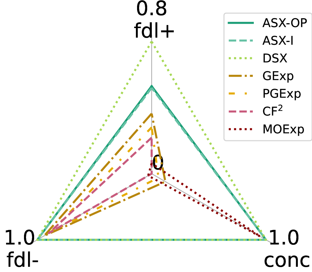
(c) MS on Cora

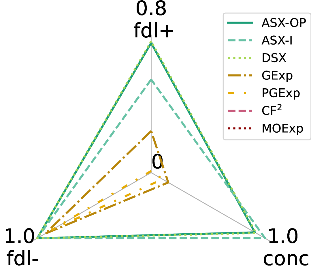
(d) MS on PubMed

Figure 3. Overall effectiveness of our skyline explanation compared to SOTA explainers ($\mathsf{GNNExplainer}$, $\mathsf{PGExplainer}$, $\mathsf{CF\textsuperscript{2}}$, $\mathsf{MOExp}$).

6.2. Experimental Results

We next present our findings.

Exp-1: Overall Explainability. We evaluate the overall performance of the $\mathsf{GNN}$ explainers using QIs.

QI-1: IPF Scores. We report IPF scores (bigger is better) for all $\mathsf{GNN}$ explainers in Figure 3(a) with $\mathsf{GCNs}$ and $k$=$10$. Additional explainability results with varying $k$ are given in the full version (ful, 2024). (1) In general, $\mathsf{ApxSX}$-$\mathsf{OP}$ outperforms a majority of competitors in aggregated explainability. For example, on $\mathsf{Cora}$, $\mathsf{ApxSX}$-$\mathsf{OP}$ outperforms $\mathsf{GNNExplainer}$, $\mathsf{PGExplainer}$, $\mathsf{CF\textsuperscript{2}}$, and $\mathsf{MOExp}$ in IPF scores by 1.34, 1.51, 2.81, and 1.79 times, respectively. $\mathsf{DivSX}$ and $\mathsf{ApxSX}$-$\mathsf{I}$ achieve comparable performance with $\mathsf{ApxSX}$-$\mathsf{OP}$. (2) We also observed that $\mathsf{GNNExplainer}$ and $\mathsf{PGExplainer}$ are sensitive as the datasets vary. For example, on $\mathsf{FacebookPage}$, both show a significant increase or decrease in IPF scores. In contrast, $\mathsf{ApxSX}$-$\mathsf{OP}$, $\mathsf{ApxSX}$-$\mathsf{I}$, and $\mathsf{DivSX}$ consistently achieve top IPF scores over all the datasets. This verifies that our methods are quite robust in generating high-quality explanations over different data sources.

QI-2: IGD Scores. Figure 3(b) reports the IGD scores (smaller is better) of the explanations for $\mathsf{GCN}$-based classification. $\mathsf{ApxSX}$-$\mathsf{OP}$, $\mathsf{ApxSX}$-$\mathsf{I}$, and $\mathsf{DivSX}$ achieve the best in IGD scores among all $\mathsf{GNN}$ explainers, for all datasets. This verifies that our explanation method is able to consistently select top explanations from a space of high-quality explanations that are separately optimized over different measures. In particular, we found that $\mathsf{ApxSX}$-$\mathsf{OP}$, $\mathsf{ApxSX}$-$\mathsf{I}$, and $\mathsf{DivSX}$ are able to “recover” the top-$k$ global optimal solutions for each individual explainability measures with high hit rates (not shown). For example, for ${\mathsf{conc}}$, at least $9$ out of $10$ are correctly and consistently identified by $\mathsf{ApxSX}$-$\mathsf{OP}$ over every dataset.

QI-3: nMX Scores. Figures 3(c) and  3(d) visualize the normalized MS scores of the $\mathsf{GNN}$ explainers, over $\mathsf{Cora}$ and $\mathsf{PubMed}$, respectively, where $k$ = $10$. (1) $\mathsf{ApxSX}$-$\mathsf{OP}$ reports a large range and contributes to explanations that are either close or the exact optimal explanation, for each of the three measures. $\mathsf{ApxSX}$-$\mathsf{I}$ and $\mathsf{DivSX}$ have comparable performance, yet with larger ranges due to its properly diversified solution. (2) $\mathsf{DivSX}$, $\mathsf{ApxSX}$-$\mathsf{OP}$, and $\mathsf{ApxSX}$-$\mathsf{I}$ contribute to the optimal ${\mathsf{fdl}}^{+}$, ${\mathsf{fdl}}^{-}$, and ${\mathsf{conc}}$, respectively. On the other hand, each individual explainer performs worse for all measures, with a large gap. For example, in $\mathsf{Cora}$, $\mathsf{MOExp}$ only achieves up to 3% of the best explanation ($\mathsf{DivSX}$) over ${\mathsf{fdl}}^{-}$.

(a) Efficiency

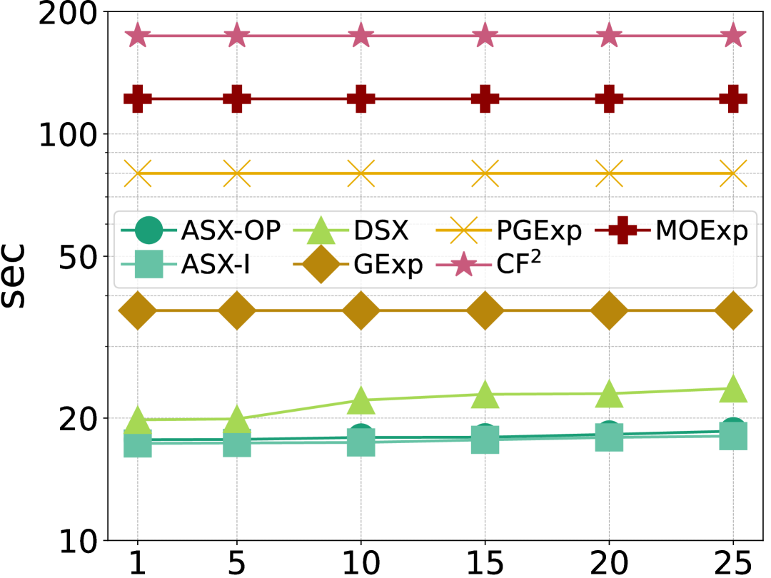
(b) Scalability w. $k$ (Cora)

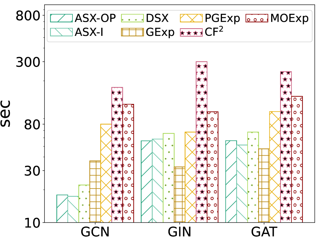
(c) Scalability w. $\mathsf{GNNs}$ (Cora)

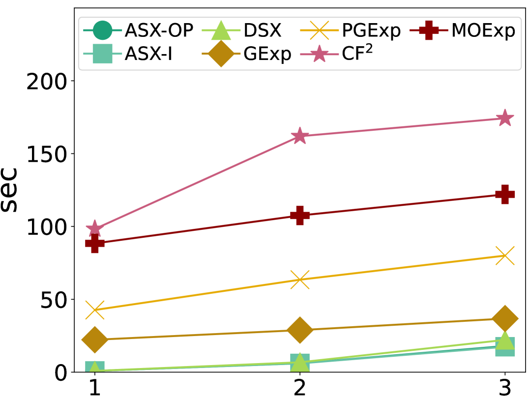
(d) Scalability w. $L$ (Cora)

Figure 4. Efficiency and scalability of our skyline explanation vs. SOTA explainers ($\mathsf{GNNExplainer}$, $\mathsf{PGExplainer}$, $\mathsf{CF\textsuperscript{2}}$, $\mathsf{MOExp}$)

Exp-2: Efficiency. Using the same setting as in Figure 3, we report the time cost. Figure 4(a) exhibits the following.

(1) $\mathsf{ApxSX}$-$\mathsf{OP}$, $\mathsf{ApxSX}$-$\mathsf{I}$, and $\mathsf{DivSX}$ outperform all (learning-based) $\mathsf{GNN}$ explanations. $\mathsf{ApxSX}$-$\mathsf{OP}$ (resp. $\mathsf{DivSX}$) on average outperforms $\mathsf{GNNExplainer}$, $\mathsf{PGExplainer}$, $\mathsf{CF\textsuperscript{2}}$, and $\mathsf{MOExp}$ by 2.05, 4.46, 9.73, 6.81 (resp. 1.62, 3.61, 7.88, and 5.51) times, respectively. Moreover, $\mathsf{ApxSX}$-$\mathsf{OP}$ supersedes $\mathsf{GNNExplainer}$ and $\mathsf{PGExplainer}$ better over larger graphs. $\mathsf{CF\textsuperscript{2}}$ and $\mathsf{MOExp}$ fail to generate explanations due to high memory cost and long waiting time. Indeed, the learning costs remain their major bottleneck as for large and dense graphs.

(2) $\mathsf{ApxSX}$-$\mathsf{OP}$, $\mathsf{ApxSX}$-$\mathsf{I}$, and $\mathsf{DivSX}$ are feasible in generating high-quality explanations for $\mathsf{GNN}$-based classification over large graphs. For example, for $\mathsf{FacebookPage}$ with 22,470 nodes and 342,004 edges, it takes $\mathsf{ApxSX}$-$\mathsf{OP}$ around $150$ seconds to generate skyline explanations with guaranteed quality. This verifies the effectiveness of its onion-peeling and optimization strategies.

(3) $\mathsf{DivSX}$ does not incur significant overhead despite that it pursues more diversified explanations. Indeed, the benefit of edge prioritization carries over to diversification process, and the incremental maintenance of the explanations reduces unnecessary verification.

(4) $\mathsf{ApxSX}$-$\mathsf{I}$ outperforms $\mathsf{ApxSX}$-$\mathsf{OP}$ for cases when the test nodes have “skewed” edge distribution in $L$-hop subgraphs, i.e., less direct neighbors but large multi-hop neighbors, which favors the edge growth strategy of $\mathsf{ApxSX}$-$\mathsf{I}$. $\mathsf{ApxSX}$-$\mathsf{OP}$ takes a relatively longer time to converge to high-quality answers via onion-peeling strategy, for nodes of interest with denser neighbors at “further” hops.

Exp-3: Scalability. We report the impact of critical factors (i.e., number of explanatory subgraphs $k$, $\mathsf{GNN}$ classes, and number of $\mathsf{GNN}$ layers $L$) on the scalability of skyline explanation generation, using $\mathsf{Cora}$ dataset. Additional experimental results about effectiveness due to varying factors are given in the full version (ful, 2024).

Varying $k$. Setting ${\mathcal{M}}$ as $\mathsf{GCN}$-based classifier with $3$ layers, we vary $k$ from 1 to 25. Since our competitors are not configurable w.r.t. $k$, we show the time costs of generating their solutions (that are independent of $k$), along with the time cost of our $\mathsf{ApxSX}$-$\mathsf{OP}$, $\mathsf{ApxSX}$-$\mathsf{I}$, and $\mathsf{DivSX}$ (which are dependent on $k$) in Figure 4(b). Our methods take longer time to maintain skyline explanation with larger $k$, as more comparisons are required per newly generated candidate. $\mathsf{DivSX}$ is relatively more sensitive to $k$ due to additional computation of cosine distances (§5), yet remains significantly faster than learning-based explainers. On average, our methods take up to 23 seconds to maintain the explanations with $k$ varied to 25.

Varying $\mathsf{GNN}$ classes and $L$. Fixing $k$=$10$, we report the time cost of $3$-layer $\mathsf{GNN}$ explainers for $\mathsf{GCN}$, $\mathsf{GAT}$, and $\mathsf{GIN}$ over $\mathsf{Cora}$. As shown in Figure 4(c), all our skyline methods take the least time to explain $\mathsf{GNN}$-based classification. This is consistent with our observation that the verification of $\mathsf{GNN}$ is the most efficient among all classes, indicating an overall small verification cost.

We fix $k$=$10$ and report the time cost of $\mathsf{GCN}$ explainers, with the number of layers $L$ varied from 1 to 3 over $\mathsf{Cora}$. Figure 4(d) shows us that all our methods significantly outperform the competitors. The learning overheads of competitors remain their major bottleneck, while our algorithms, as post-hoc explainers without learning overhead, are more efficient. As expected, all our methods take a longer time to generate explanations for larger $L$, as more subgraphs need to be verified from larger induced $L$-hop neighbors.

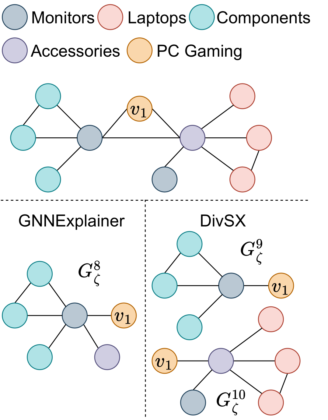
(a) Skyline Explanation v.s. $\mathsf{GNNExplainer}$ ($\mathsf{AmazonComputer}$)

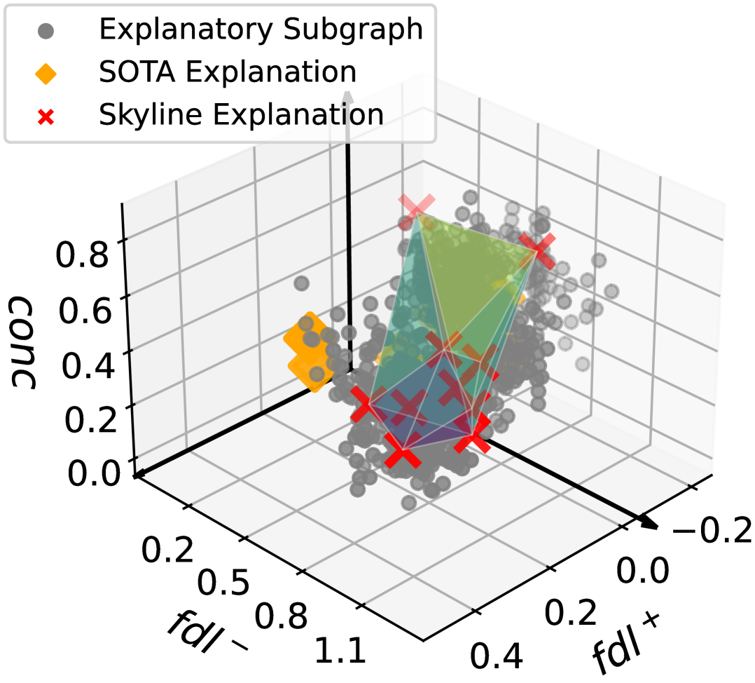
(b) Visualization of Skyline Explanation ($\mathsf{AmazonComputer}$)

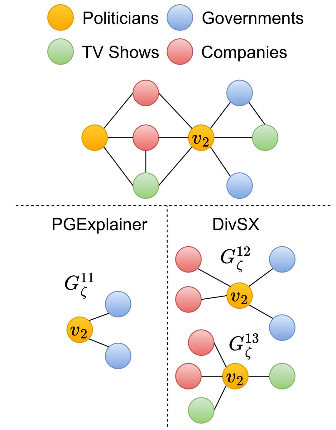
(c) Skyline Explanation v.s. $\mathsf{PGExplainer}$ ($\mathsf{FacebookPage}$)

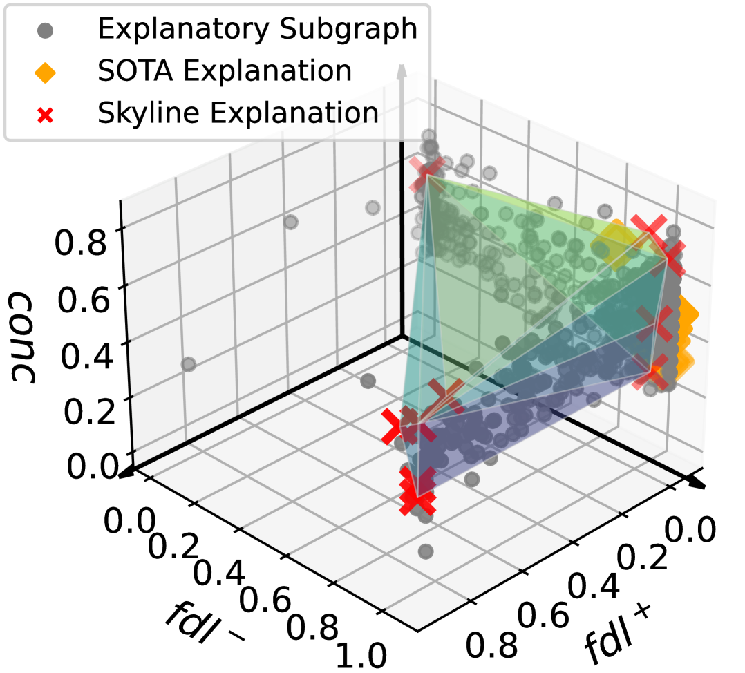
(d) Visualization of Skyline Explanation ($\mathsf{FacebookPage}$)

Figure 5. Qualitative analysis of our skyline explanation compared to SOTA explainers ($\mathsf{GNNExplainer}$, $\mathsf{PGExplainer}$, $\mathsf{CF\textsuperscript{2}}$, $\mathsf{MOExp}$)

Exp-4: Case Analysis. We next showcase qualitative analyses of our explanation methods, using real-world examples from two datasets: $\mathsf{AmazonComputer}$ and $\mathsf{FacebookPage}$.

Diversified Explanation. A user is interested in finding “Why” a product $v_{1}$ is labeled “PC Gaming” by a $\mathsf{GCN}$. $\mathsf{GNN}$ explainers that optimize a single measure (e.g.,   $\mathsf{GNNExplainer}$) return explanations (see $G_{\zeta}^{8}$ in Figure 5(a)) that simply reveals a fact that $v_{1}$ is co-purchased with “Components”, a “one-sided” interpretation. In contrast, $\mathsf{DivSX}$ identifies an explanation that reveals more comprehensive interpretation with two explanatory subgraphs (both factual) $\{G_{\zeta}^{9},G_{\zeta}^{10}\}$ (Figure 5(a)), which reveal two co-purchasing patterns bridging $v_{1}$ with not only “Components” for “Monitors” (by $G_{\zeta}^{9}$), but also to “Accessories” of “Laptops”. Indeed, a closer inspection confirms that the former indicates gamers who prefer building their gaming PC with high-refresh rate monitors designed for gaming ; and the latter indicates that $v_{1}$ is a gaming laptop which needs frequent maintenance with laptop accessories. This verifies that $\mathsf{DivSX}$ is able to provide more comprehensive explanation.

In Figure 5(b), we visualize the distribution of explanatory subgraphs of $v_{1}$ from Figure 5(a). Each point in the plot denotes an explanatory subgraph with $3D$ coordinates from normalized ${\mathsf{fdl}}^{+}$, ${\mathsf{fdl}}^{-}$, and ${\mathsf{conc}}$ scores. The verified interpretable space includes all the gray dots, the explanatory subgraphs generated by state-of-the-art (SOTA) explainers (i.e., $\mathsf{GNNExplainer}$, $\mathsf{PGExplainer}$, $\mathsf{CF\textsuperscript{2}}$, $\mathsf{MOExp}$) are highlighted as “diamond” points. Our skyline explanation is highlighted with red crosses. We visualize the convex hull based on skyline points to showcase their dominance over other explanatory subgraphs. We observe that the skyline explanation covers most of the interpretable space and provides comprehensive and diverse explanations. On the other hand, SOTA explainers often localize their solutions in smaller regions of the interpretable space, therefore missing diverse explanations (Das and Dennis, 1997).

Skyline vs. Multi-objective Explanation via Linear Combination. Our second case compares $\mathsf{DivSX}$ and $\mathsf{PGExplainer}$ (shown in Figure 5(c)). The latter generates explanations by optimizing a single objective that combines two explanation measures (factuality and conciseness). We observe that $\mathsf{PGExplainer}$ generates small factual subgraphs, such as $G_{\zeta}^{11}$ for a test node $v_{2}$, yet relatively less informative. $\mathsf{DivSX}$ generates a skyline explanation $\{G_{\zeta}^{12},G_{\zeta}^{13}\}$ that is able to interpret $v_{2}$ as “Politicians” not only due to its connection with “Governments” entities but also highly related to “TV shows” and “Companies”. Meanwhile, Figure 5(d) verifies that our skyline explanation covers most of the interpretable space with diverse and comprehensive explanations, while the SOTA explainers cluster their solutions in smaller regions.

We have also compared $\mathsf{ApxSX}$-$\mathsf{OP}$ and $\mathsf{ApxSX}$-$\mathsf{I}$ with their applications. Due to limited space, we present the details in (ful, 2024).

7. Conclusion

We have proposed a class of skyline explanations that simultaneously optimize multiple explainability measures for $\mathsf{GNN}$ explanation. We have shown that the generation of skyline explanations in terms of Pareto optimality remains nontrivial even for polynomially bounded input space and three measures. We have introduced feasible algorithms for skyline explanation generation problem as well as its diversified counterpart, with provable quality guarantees in terms of Pareto optimality. Our experimental study has verified that our methods are practical for large-scale graphs and $\mathsf{GNN}$-based classification and generate more comprehensive explanations, compared with state-of-the-art $\mathsf{GNN}$ explainers. A future topic is to develop distributed algorithms for skyline explanation generation.

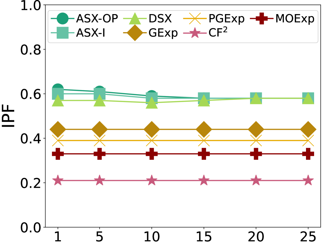
(a) IPF varying $k$

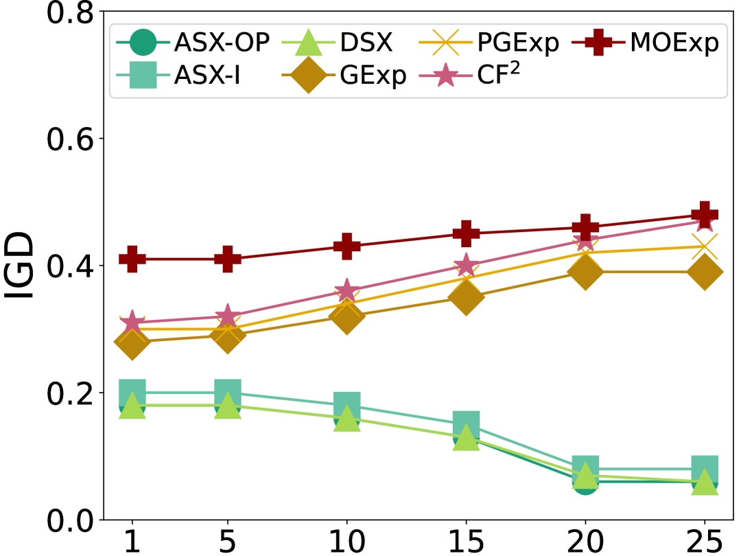
(b) IGD varying $k$

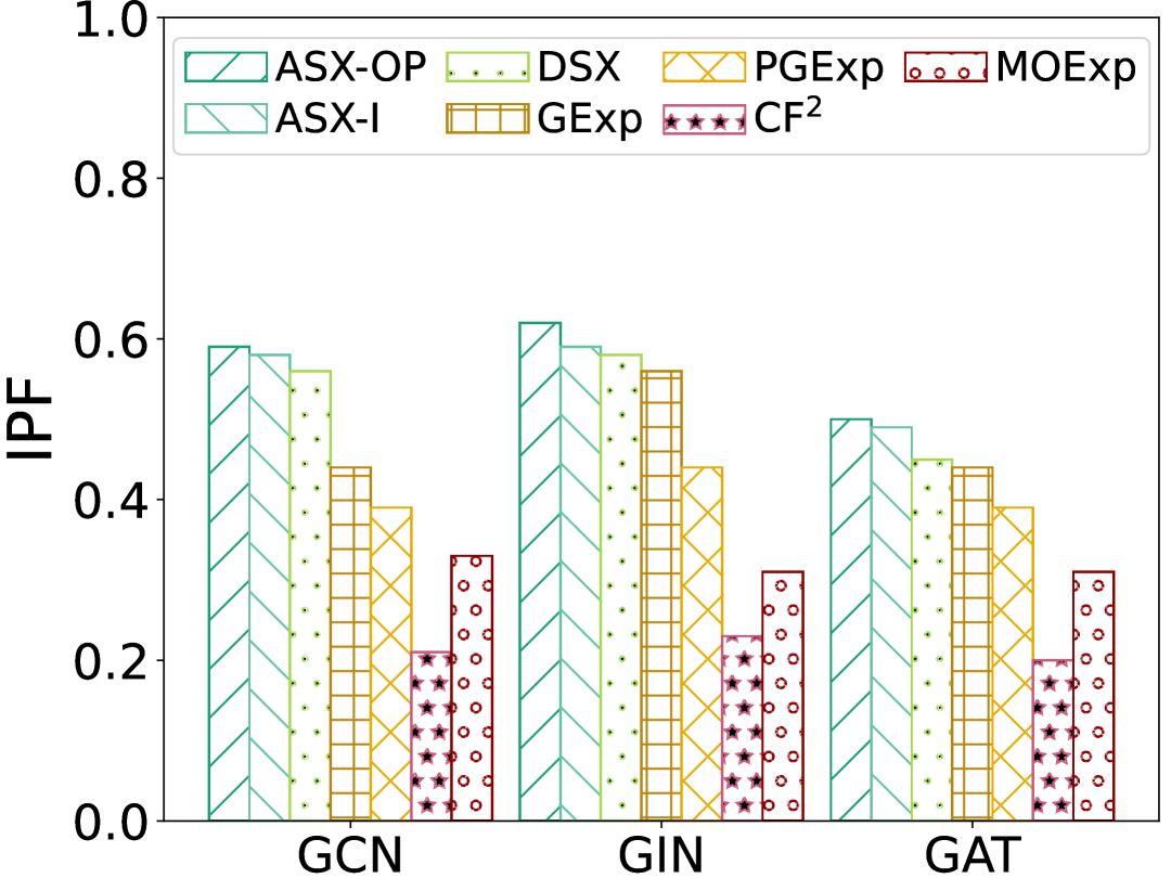
(c) IPF varying $\mathsf{GNNs}$

(d) IGD varying $L$

Figure 6. Impact of factors on the effectiveness of explanations

Appendix

7.1. Additional Algorithmic Details

Update Dominance Relationships. We introduce the details of Procedure updateSX. With the stream of upcoming states, i.e., explanatory subgraphs, we maintain a lattice structure for the dominance relationships. Specifically, we first compare the new state $s$ with the current skylines: 1) If certain skylines dominate it, we connect a directed edge from these dominating skylines to the new state, respectively. 2) If the new state dominates certain skylines, we connect directed edges from the new state to these dominated skylines. Meanwhile, we reconnect the dominant states of these skylines to the new state. 3) If the new state is not dominated by any skylines, then we obtain its ${\mathcal{D}}(s)$ using the bitvector $B(s)$. Next, we identify the skyline $\overline{s}$ with the smallest ${\mathcal{D}}(\overline{s})$, replace $\overline{s}$ with $s$, only when such replacement makes the ${\mathcal{D}}$ increased by a factor of $\frac{1}{k}$. If swapping is conducted, the new skyline, i.e. $s$, connects directed edges to the dominating states based on bitvector $B(s)$, and we remove the swapped skyline and its corresponding edges. The above swap strategy ensures a $\frac{1}{4}$-approximation ratio (Ausiello et al., 2012).

Alternative Strategy: Edge Growing. Edge growing strategy differs from the “onion peeling” strategy with the test node as the initial state and the $L$-hop neighbor subgraph as the final state. $\mathsf{ApxSX}$-$\mathsf{I}$ adopts Breadth-First Search to explore explanatory subgraphs. Specifically, starting from the test node, we first connect the test node with each of its neighbors, respectively. Then we verify these candidate subgraphs and determine the ($1+\epsilon$)-dominance relationships. Following the same candidate prioritization as $\mathsf{ApxSX}$-$\mathsf{OP}$, we select the neighboring node with the biggest weight. Then, continuing with this newly chosen node, we explore its neighbors, except the ones that we previously visited. We expand the subgraph with the neighbors, respectively, and conduct candidate prioritization again. We iteratively continue this process until we explore the explanatory subgraph as the $L$- neighbor subgraph. The search space and time complexity of $\mathsf{ApxSX}$-$\mathsf{I}$ remains the same as $\mathsf{ApxSX}$-$\mathsf{OP}$, since the interpretation domain $\zeta^{\prime}$ and the update strategy are the same.

Diversification Algorithm. The detailed pseudo-codes of diversification algorithm $\mathsf{DivSX}$ are shown as Algorithm 3 and Procedure 4. Please find the detailed descriptions of $\mathsf{DivSX}$ in § 5.

Algorithm 3 $\mathsf{DivSX}$ Algorithm

0: a query ${\mathsf{SXQ}}^{k}$ = $(G,{\mathcal{M}},V_{T},\Phi)$; a constant $\epsilon\in[0,1]$;

0: a $(\zeta^{\prime},\epsilon)$-explanation ${\mathcal{G}}_{\epsilon}$.

1: set ${\mathcal{G}}_{\epsilon}$ := $\emptyset$;

2: identify edges for each hop: ${\mathcal{E}}$=$\{E_{L},E_{L-1},\ldots,E_{1}\}$;

3: for $l$ = $L$ to $1$ do # Generator: Onion Peeling

4:  initializes state $s_{0}=G^{l}(V_{T})$ ($l$-hop neighbor subgraph).

5:  while $E_{l}\neq\emptyset$ do

6:   for $e\in E_{l}$ do

7:    spawns a state $s$ with a candidate $G_{s}$ := $G^{l}\backslash\{e\}$;

8:    update $\zeta^{\prime}$ with state $s$ and a new transaction $t$;

9:    if ${\sf vrfyF}(s)$=False & ${\sf vrfyCF}(s)$=False then # Verifier

10:     continue;

11:    ${\mathcal{G}}_{\epsilon}$ :=updateDivSX $(s,G_{s},\zeta^{\prime},{\mathcal{G}}_{\epsilon})$; $E_{l}$=$E_{l}\backslash\{e\}$; # Updater

12: return  ${\mathcal{G}}_{\epsilon}$.

Procedure 4 Procedure updateDivSX

0: a state $s$, an explanatory subgraph $G_{s}$, state graph $\zeta^{\prime}$; an explanation ${\mathcal{G}}_{\epsilon}$;

0: Updated $(\zeta^{\prime},\epsilon)$-explanation ${\mathcal{G}}_{\epsilon}$;

1: initializes state $s$ with structure $\Phi(G_{s})$:=$\emptyset$;

2: evaluates $\Phi(G_{s})$;

3: incrementally determines $(1+\epsilon)$-dominance of $G_{s}$;

4: if $\{G_{s}\}$ is a new skyline explanation then # New skyline

5:  $\Delta(s|{\mathcal{G}}_{\epsilon})$ := ${\sf DivS}($${\mathcal{G}}_{\epsilon}$$\cup$$\{G_{s}\}$$)-{\sf DivS}($${\mathcal{G}}_{\epsilon}$$)$

6:  if $|{\mathcal{G}}_{\epsilon}|$$<$$k$ and $\Delta(s|{\mathcal{G}}_{\epsilon})$$\geq$$\frac{(1+\epsilon)/2-{\sf DivS}({\mathcal{G}}_{\epsilon})}{k-|{\mathcal{G}}_{\epsilon}|}$ then

7:   ${\mathcal{G}}_{\epsilon}$ := ${\mathcal{G}}_{\epsilon}$$\cup$$\{G_{s}\}$;

8: return  ${\mathcal{G}}_{\epsilon}$.

7.2. Additional Experimental Results

Impact of Factors. We report the impact of critical factors, i.e., size of explanations $k$, $\mathsf{GNN}$ classes, and the number of layers $L$, on the effectiveness of generated skyline explanation over the $\mathsf{Cora}$ dataset.

Impact of $k$. Setting ${\mathcal{M}}$ as $\mathsf{GCN}$-based classifier with $3$ layers, we vary $k$ from 1 to 25. Since our competitors are not configurable w.r.t. $k$, we show the IPF and IGD scores of their solutions (that are independent of $k$), along with our $\mathsf{ApxSX}$-$\mathsf{OP}$, $\mathsf{ApxSX}$-$\mathsf{I}$, and $\mathsf{DivSX}$ (which are dependent on $k$) in Figures 6(a) and 6(b). As $k$ becomes larger, $\mathsf{ApxSX}$-$\mathsf{OP}$, $\mathsf{ApxSX}$-$\mathsf{I}$, and $\mathsf{DivSX}$ all achieve better scores and are able to consistently generate explanations with higher quality. This is because larger $k$ allows more dominating subgraphs to be verified, whenever possible for at least one measure. In contrast, our competitors are not aware of the growth of $k$, given that they may “stuck” at local optimal explanations that are optimized over a single measure, hence fail to improve the solution even with larger $k$. Moreover, $\mathsf{MOExp}$ does not explicitly constrain the size of the explanation set, which can result up to 200 explanatory subgraphs based on our empirical results. Meanwhile, even with $k$=$1$, our three methods achieve the highest scores in both IPF and IGD, compared to our competitors.

Varying $\mathsf{GNN}$ classes. Fixing $k$=$10$, we report IPF scores of $3$-layer $\mathsf{GNN}$ explainers for representative $\mathsf{GNN}$ classes including $\mathsf{GCN}$, $\mathsf{GAT}$, and $\mathsf{GIN}$. As verified in Figure 6(c), $\mathsf{ApxSX}$-$\mathsf{OP}$, $\mathsf{ApxSX}$-$\mathsf{I}$, and $\mathsf{DivSX}$ consistently outperform other explanations for different $\mathsf{GNN}$ classes. This verifies that our approaches remain stable in generating high-quality explanations for different types of $\mathsf{GNNs}$. Our observations for IGD scores are consistent, hence omitted.

Varying number of layers. Fixing $k$=$10$, we report IGD scores of $\mathsf{GCN}$ explainers, with the number of layer $L$ varies from 1 to 3. over $\mathsf{Cora}$. Fig 6(d) shows that $\mathsf{ApxSX}$-$\mathsf{OP}$, $\mathsf{ApxSX}$-$\mathsf{I}$, and $\mathsf{DivSX}$ are able to achieve better IGD scores for generating explanations with more complex $\mathsf{GNNs}$ having “deeper” architecture. Indeed, as $L$ becomes larger, our all three methods are able to identify more connected subgraphs that contribute to better ${\mathsf{fdl}}^{+}$ and ${\mathsf{fdl}}^{-}$ scores, hence improving explanation quality.

Figure 7. Different edge explore strategies show different preferences for returned skyline explanation.

Case Study: Insertion v.s. Onion-Peeling. In this case study, we compare the application scenarios of $\mathsf{ApxSX}$-$\mathsf{OP}$ and $\mathsf{ApxSX}$-$\mathsf{I}$, as shown in Figure 7. We observe that $\mathsf{ApxSX}$-$\mathsf{OP}$, with onion peeling, cater users’ needs who “think slow” and seeks in-depth explanations that are counterfactual. Such larger and counterfactual explanations are more likely to affect $\mathsf{GNN}$ behaviors if removed (Liu et al., 2021). $\mathsf{ApxSX}$-$\mathsf{I}$, on the other hand, due to its containment of edges closer to targeted ones via edge insertions, tends to produce – at its early stage – smaller, factual explanations as convincing evidences. This caters users who “think fast” and is good at quick generation of factual explanations (Liu et al., 2021). For example, in answering “why” node $v^{\prime}_{t}$ is recognized as a “Politician” site, $G_{\zeta}^{8}$ and $G_{\zeta}^{9}$ are among skyline explanations from $\mathsf{ApxSX}$-$\mathsf{I}$ at early stage, revealing the fact that $v^{\prime}_{t}$ frequently interact with TV shows, Governments, and Companies, covering its ego-networks as quick facts. $G_{\zeta}^{10}$ and $G_{\zeta}^{11}$, which are reported by $\mathsf{ApxSX}$-$\mathsf{OP}$ in its early stage via “onion-peeling”, are relatively larger counterfactual explanations that suggest interaction patterns with more complex structures. For example, $G_{\zeta}^{11}$ includes two-hop neighbors and a triangle, which indicates the importance of the corresponding company and TV show. Most importantly, another politician’s two-hop neighbor also shares these nodes, revealing the close relationship between the two politicians.

References

- (1)
- cod (2024) 2024. Code and datasets. https://github.com/DazhuoQ/SkyExp.
- ful (2024) 2024. Full version. https://github.com/DazhuoQ/SkyExp_full_version.
- Ausiello et al. (2012) Giorgio Ausiello, Nicolas Boria, Aristotelis Giannakos, Giorgio Lucarelli, and Vangelis Th. Paschos. 2012. Online maximum k-coverage. Discrete Applied Mathematics 160, 13 (2012), 1901–1913.
- Badanidiyuru et al. (2014) Ashwinkumar Badanidiyuru, Baharan Mirzasoleiman, Amin Karbasi, and Andreas Krause. 2014. Streaming submodular maximization: massive data summarization on the fly. In ACM SIGKDD International Conference on Knowledge Discovery and Data Mining. 671–680.
- Bellei et al. (2024) Claudio Bellei, Muhua Xu, Ross Phillips, Tom Robinson, Mark Weber, Tim Kaler, Charles E. Leiserson, Arvind, and Jie Chen. 2024. The shape of money laundering: Subgraph representation learning on the blockchain with the Elliptic2 dataset. In KDD Workshop on Machine Learning in Finance.
- Börzsönyi et al. (2001) Stephan Börzsönyi, Donald Kossmann, and Konrad Stocker. 2001. The skyline operator. In International Conference on Data Engineering (ICDE). 421–430.
- Cai et al. (2021) Xinye Cai, Yushun Xiao, Miqing Li, Han Hu, Hisao Ishibuchi, and Xiaoping Li. 2021. A grid-based inverted generational distance for multi/many-objective optimization. IEEE Transactions on Evolutionary Computation 25, 1 (2021), 21–34.
- Carlyle et al. (2003) W Matthew Carlyle, John W Fowler, Esma S Gel, and Bosun Kim. 2003. Quantitative comparison of approximate solution sets for bi-criteria optimization problems. Decision Sciences 34, 1 (2003), 63–82.
- Chan et al. (2006) Chee-Yong Chan, H. V. Jagadish, Kian-Lee Tan, Anthony K. H. Tung, and Zhenjie Zhang. 2006. Finding k-dominant skylines in high dimensional space. In ACM SIGMOD International Conference on Management of Data. 503–514.
- Chen et al. (2020) Ming Chen, Zhewei Wei, Bolin Ding, Yaliang Li, Ye Yuan, Xiaoyong Du, and Ji-Rong Wen. 2020. Scalable graph neural networks via bidirectional propagation. In Advances in Neural Information Processing Systems (NeurIPS).
- Chen et al. (2024) Tingyang Chen, Dazhuo Qiu, Yinghui Wu, Arijit Khan, Xiangyu Ke, and Yunjun Gao. 2024. View-based explanations for graph neural networks. Proc. ACM Manag. Data 2, 1 (2024), 40:1–40:27.
- Cheng et al. (2023) Ling Cheng, Feida Zhu, Yong Wang, Ruicheng Liang, and Huiwen Liu. 2023. Evolve path tracer: Early detection of malicious addresses in cryptocurrency. In ACM SIGKDD Conference on Knowledge Discovery and Data Mining. 3889–3900.
- Chircop and Zammit-Mangion (2013) Kenneth Chircop and David Zammit-Mangion. 2013. On e-constraint based methods for the generation of Pareto frontiers. Journal of Mechanics Engineering and Automation (2013), 279–289.
- Cho et al. (2011) Eunjoon Cho, Seth A. Myers, and Jure Leskovec. 2011. Friendship and mobility: User movement in location-based social networks. In ACM SIGKDD International Conference on Knowledge Discovery and Data Mining. 1082–1090.
- Chomicki et al. (2013) Jan Chomicki, Paolo Ciaccia, and Niccolo’ Meneghetti. 2013. Skyline queries, front and back. SIGMOD Rec. 42, 3 (oct 2013), 6–18.
- Ciaccia and Martinenghi (2017) Paolo Ciaccia and Davide Martinenghi. 2017. Reconciling skyline and ranking queries. Proc. VLDB Endow. 10, 11 (2017), 1454–1465.
- Coello Coello and Reyes Sierra (2004) Carlos A Coello Coello and Margarita Reyes Sierra. 2004. A study of the parallelization of a coevolutionary multi-objective evolutionary algorithm. In MICAI 2004: Advances in Artificial Intelligence: Third Mexican International Conference on Artificial Intelligence. Proceedings 3. 688–697.
- Das and Dennis (1997) Indraneel Das and John E Dennis. 1997. A closer look at drawbacks of minimizing weighted sums of objectives for Pareto set generation in multicriteria optimization problems. Structural optimization 14 (1997), 63–69.
- Elmougy and Liu (2023) Youssef Elmougy and Ling Liu. 2023. Demystifying fraudulent transactions and illicit nodes in the Bitcoin network for financial forensics. In ACM SIGKDD Conference on Knowledge Discovery and Data Mining. 3979–3990.
- Fan et al. (2019) Wenqi Fan, Yao Ma, Qing Li, Yuan He, Eric Zhao, Jiliang Tang, and Dawei Yin. 2019. Graph neural networks for social recommendation. In The World Wide Web Conference (WWW). 417–426.
- Fortunato (2010) Santo Fortunato. 2010. Community detection in graphs. Physics reports 486, 3-5 (2010), 75–174.
- Geerts (2023) Floris Geerts. 2023. A query language perspective on graph learning. In ACM SIGMOD-SIGACT-SIGAI Symposium on Principles of Database Systems (PODS). 373–379.
- Grover and Leskovec (2016) Aditya Grover and Jure Leskovec. 2016. node2vec: Scalable feature learning for networks. In ACM SIGKDD international conference on Knowledge discovery and data mining. 855–864.
- He et al. (2022) Haoyu He, Yuede Ji, and H. Howie Huang. 2022. Illuminati: Towards explaining graph neural networks for cybersecurity analysis. In IEEE European Symposium on Security and Privacy. 74–89.
- Hu et al. (2020) Weihua Hu, Matthias Fey, Marinka Zitnik, Yuxiao Dong, Hongyu Ren, Bowen Liu, Michele Catasta, and Jure Leskovec. 2020. Open graph benchmark: Datasets for machine learning on graphs. In Advances in neural information processing systems (NeurIPS).
- Hwang and Masud (1979) Ching-Lai Hwang and Abu Syed Md Masud. 1979. Multiple objective decision making—methods and applications: a state-of-the-art survey. Springer-Verlag.
- Karakashian et al. (2013) Shant Karakashian, Berthe Y Choueiry, and Stephen G Hartke. 2013. An algorithm for generating all connected subgraphs with k vertices of a graph. Lincoln, NE 10, 2505515.2505560 (2013).
- Kipf and Welling (2016) Thomas N Kipf and Max Welling. 2016. Semi-supervised classification with graph convolutional networks. In International Conference on Learning Representations (ICLR).
- Kung et al. (1975) H. T. Kung, Fabrizio Luccio, and Franco P. Preparata. 1975. On finding the maxima of a set of vectors. J. ACM 22, 4 (1975), 469–476.
- Laumanns et al. (2002) Marco Laumanns, Lothar Thiele, Eckart Zitzler, and Kalyanmoy Deb. 2002. Archiving with guaranteed convergence and diversity in multi-objective optimization. In Genetic and Evolutionary Computation Conference (GECCO). 439–447.
- Li and Yao (2019) Miqing Li and Xin Yao. 2019. Quality evaluation of solution sets in multiobjective optimisation: A survey. ACM Computing Surveys (CSUR) 52, 2 (2019), 1–38.
- Lin et al. (2006) Xuemin Lin, Yidong Yuan, Qing Zhang, and Ying Zhang. 2006. Selecting stars: The k most representative skyline operator. In International Conference on Data Engineering (ICDE). 86–95.
- Liu et al. (2021) Yifei Liu, Chao Chen, Yazheng Liu, Xi Zhang, and Sihong Xie. 2021. Multi-objective explanations of GNN predictions. In IEEE International Conference on Data Mining (ICDM). 409–418.
- Lucic et al. (2022) Ana Lucic, Maartje A Ter Hoeve, Gabriele Tolomei, Maarten De Rijke, and Fabrizio Silvestri. 2022. Cf-gnnexplainer: Counterfactual explanations for graph neural networks. In International Conference on Artificial Intelligence and Statistics (AISTATS). 4499–4511.
- Luo et al. (2020) Dongsheng Luo, Wei Cheng, Dongkuan Xu, Wenchao Yu, Bo Zong, Haifeng Chen, and Xiang Zhang. 2020. Parameterized explainer for graph neural network. In Advances in Neural Information Processing Systems (NeurIPS).
- Marler and Arora (2010) R Timothy Marler and Jasbir S Arora. 2010. The weighted sum method for multi-objective optimization: new insights. Structural and multidisciplinary optimization 41 (2010), 853–862.
- McCallum et al. (2000) Andrew Kachites McCallum, Kamal Nigam, Jason Rennie, and Kristie Seymore. 2000. Automating the construction of internet portals with machine learning. Information Retrieval 3 (2000), 127–163.
- Morales-Hernández et al. (2022) Alejandro Morales-Hernández, Inneke Van Nieuwenhuyse, and Sebastian Rojas Gonzalez. 2022. A survey on multi-objective hyperparameter optimization algorithms for machine learning. Artif. Intell. Rev. 56, 8 (2022), 8043–8093.
- Ouyang et al. (2024) Shiyu Ouyang, Qianlan Bai, Hui Feng, and Bo Hu. 2024. Bitcoin money laundering detection via subgraph contrastive learning. Entropy 26, 3 (2024).
- Papadias et al. (2003) Dimitris Papadias, Yufei Tao, Greg Fu, and Bernhard Seeger. 2003. An optimal and progressive algorithm for skyline queries. In ACM SIGMOD International Conference on Management of Data. 467–478.
- Papadimitriou and Yannakakis (2000) Christos H. Papadimitriou and Mihalis Yannakakis. 2000. On the approximability of trade-offs and optimal access of Web sources. In Annual Symposium on Foundations of Computer Science, (FOCS). 86–92.
- Peng and Wong (2018) Peng Peng and Raymond Chi-Wing Wong. 2018. Skyline queries and pareto optimality. In Encyclopedia of Database Systems, Second Edition. Springer.
- Pocher et al. (2023) Nadia Pocher, Mirko Zichichi, Fabio Merizzi, Muhammad Zohaib Shafiq, and Stefano Ferretti. 2023. Detecting anomalous cryptocurrency transactions: An AML/CFT application of machine learning-based forensics. Electronic Markets 33, 1 (2023), 37.
- Pushpakom et al. (2019) Sudeep Pushpakom, Francesco Iorio, Patrick A Eyers, K Jane Escott, Shirley Hopper, Andrew Wells, Andrew Doig, Tim Guilliams, Joanna Latimer, Christine McNamee, Alan Norris, Philippe Sanseau, David Cavalla, and Munir Pirmohamed. 2019. Drug repurposing: progress, challenges and recommendations. Nature reviews Drug discovery 18, 1 (2019), 41–58.
- Qiu et al. (2024) Dazhuo Qiu, Mengying Wang, Arijit Khan, and Yinghui Wu. 2024. Generating robust counterfactual witnesses for graph neural networks. In IEEE International Conference on Data Engineering (ICDE). 3351–3363.
- Rozemberczki et al. (2021) Benedek Rozemberczki, Carl Allen, and Rik Sarkar. 2021. Multi-scale attributed node embedding. Journal of Complex Networks 9, 2 (2021).
- Schlichtkrull et al. (2020) Michael Sejr Schlichtkrull, Nicola De Cao, and Ivan Titov. 2020. Interpreting graph neural networks for NLP with differentiable edge masking. In International Conference on Learning Representations (ICLR).
- Schütze and Hernández (2021) Oliver Schütze and Carlos Hernández. 2021. Computing -(approximate) pareto fronts. In Archiving Strategies for Evolutionary Multi-objective Optimization Algorithms. 41–66.
- Sen et al. (2008) Prithviraj Sen, Galileo Namata, Mustafa Bilgic, Lise Getoor, Brian Gallagher, and Tina Eliassi-Rad. 2008. Collective classification in network data. AI Magazine 29, 3 (2008), 93–106.
- Sharma and Kumar (2022) Shubhkirti Sharma and Vijay Kumar. 2022. A comprehensive review on multi-objective optimization techniques: Past, present and future. Archives of Computational Methods in Engineering 29, 7 (2022), 5605–5633.
- Shchur et al. (2018) Oleksandr Shchur, Maximilian Mumme, Aleksandar Bojchevski, and Stephan Günnemann. 2018. Pitfalls of graph neural network evaluation. In Relational Representation Learning Workshop @ NeurIPS.
- Tan et al. (2022) Juntao Tan, Shijie Geng, Zuohui Fu, Yingqiang Ge, Shuyuan Xu, Yunqi Li, and Yongfeng Zhang. 2022. Learning and evaluating graph neural network explanations based on counterfactual and factual reasoning. In ACM web conference (WWW). 1018–1027.
- Tsaggouris and Zaroliagis (2009) George Tsaggouris and Christos Zaroliagis. 2009. Multiobjective optimization: Improved FPTAS for shortest paths and non-linear objectives with applications. Theory of Computing Systems 45, 1 (2009), 162–186.
- Velickovic et al. (2018) Petar Velickovic, Guillem Cucurull, Arantxa Casanova, Adriana Romero, Pietro Liò, and Yoshua Bengio. 2018. Graph attention networks. In International Conference on Learning Representations (ICLR).
- Wang et al. (2023) Yuyang Wang, Zijie Li, and Amir Barati Farimani. 2023. Graph neural networks for molecules. Springer International Publishing, 21–66.
- Wei et al. (2023) Lanning Wei, Huan Zhao, Zhiqiang He, and Quanming Yao. 2023. Neural architecture search for GNN-based graph classification. ACM Trans. Inf. Syst. 42, 1 (2023).
- Xu et al. (2019) Keyulu Xu, Weihua Hu, Jure Leskovec, and Stefanie Jegelka. 2019. How powerful are graph neural networks?. In International Conference on Learning Representations (ICLR).
- Xue et al. (2022) Ke Xue, Jiacheng Xu, Lei Yuan, Miqing Li, Chao Qian, Zongzhang Zhang, and Yang Yu. 2022. Multi-agent dynamic algorithm configuration. In Advances in Neural Information Processing Systems (NeurIPS).
- Yang et al. (2021) Zhengyi Yang, Longbin Lai, Xuemin Lin, Kongzhang Hao, and Wenjie Zhang. 2021. HUGE: An efficient and scalable subgraph enumeration system. In International Conference on Management of Data (SIGMOD).
- Ying et al. (2019) Zhitao Ying, Dylan Bourgeois, Jiaxuan You, Marinka Zitnik, and Jure Leskovec. 2019. GNNExplainer: Generating explanations for graph neural networks. In Advances in Neural Information Processing Systems (NeurIPS).
- You et al. (2018) Jiaxuan You, Bowen Liu, Rex Ying, Vijay Pande, and Jure Leskovec. 2018. Graph convolutional policy network for goal-directed molecular graph generation. In Advances in Neural Information Processing Systems (NeurIPS).
- Yuan et al. (2023) Hao Yuan, Haiyang Yu, Shurui Gui, and Shuiwang Ji. 2023. Explainability in graph neural networks: A taxonomic survey. IEEE Transactions on Pattern Analysis and Machine Intelligence 45, 5 (2023), 5782–5799.
- Yuan et al. (2021) Hao Yuan, Haiyang Yu, Jie Wang, Kang Li, and Shuiwang Ji. 2021. On explainability of graph neural networks via subgraph explorations. In International conference on machine learning (ICLR).
- Zhang and Chen (2018) Muhan Zhang and Yixin Chen. 2018. Link prediction based on graph neural networks. In Advances in neural information processing systems (NerIPS).
- Zhang et al. (2022) Shichang Zhang, Yozen Liu, Neil Shah, and Yizhou Sun. 2022. Gstarx: Explaining graph neural networks with structure-aware cooperative games. In Advances in Neural Information Processing Systems (NeurIPS).
- Zhang et al. (2024) Youmin Zhang, Qun Liu, Guoyin Wang, William K Cheung, and Li Liu. 2024. GEAR: Learning graph neural network explainer via adjusting gradients. Knowledge-Based Systems 302 (2024), 112368.