Second-gradient models for incompressible viscous fluids and associated cylindrical flows
Abstract.
We introduce second-gradient models for incompressible viscous fluids, building on the framework introduced by Fried and Gurtin. We propose a new and simple constitutive relation for the hyperpressure to ensure that the models are both physically meaningful and mathematically well-posed. The framework is further extended to incorporate pressure-dependent viscosities. We show that for the pressure-dependent viscosity model, the inclusion of second-gradient effects guarantees the ellipticity of the governing pressure equation, in contrast to previous models rooted in classical continuum mechanics. The constant viscosity model is applied to steady cylindrical flows, where explicit solutions are derived under both strong and weak adherence boundary conditions. In each case, we establish convergence of the velocity profiles to the classical Navier-Stokes solutions as the model’s characteristic length scales tend to zero.
1. Introduction
1.1. Higher-gradient continua
This work introduces second-gradient models for incompressible viscous fluids including those with pressure-dependent viscosities. Here, “second-gradient” refers to the highest order of spatial derivatives of the velocity appearing in the internal power expenditures. The general model introduced in [16] contains an internal ambiguity (outlined in Section 1.2) that restricts its predictive capability. The aim of this paper is to resolve this issue and to develop physically meaningful and mathematically well-posed theories that extend the classical incompressible Navier–Stokes model into regimes where it breaks down, including small-length scale flows and high-pressure flows exhibiting pressure-dependent viscosities; see [36, 35, 42, 48, 61, 62] and Bridgman’s Nobel Prize winning work [7, 8, 47].
In classical continuum mechanics, only the first gradient of the spatial velocity appears in the internal power expended during the motion, and models do not possess internal length scales. The idea of continua with internal power or work expenditures depending on second- and higher-order spatial derivatives of the motion was first conceived by Piola in 1846 [49, 12]. Later, the Cosserat brothers [10] introduced additional degrees of freedom at each material point, represented by an orthonormal frame parameterizing a rigid microstructure. However, major advances in generalized continuum theories incorporating small-length scale effects did not occur until the latter half of the 20th century, through foundational work by Toupin [59, 60], Green and Rivlin [26, 25], Mindlin [43, 44], Mindlin and Eshel [45], and Germain [19, 20]. These efforts culminated in general theories of gradient and micromorphic continua characterized by possibly multiple intrinsic length scales (see, e.g., [2, 40, 41, 13, 39, 14, 6]).
1.2. Fried-Gurtin model of second-gradient incompressible linear viscous fluids
The models developed here builds upon a general framework for incompressible linear viscous fluids introduced in [16]. In particular, an additional third-order hyperstress tensor is introduced alongside the classical Cauchy stress tensor , with dual to the second gradient of the spatial velocity in the internal power expenditure111For a discussion of our notation, see Section 2.1.
| (1.1) |
The resulting governing equations are
| (1.2) |
where is the constant mass density, a specific external body force, and the specific inertial body force; see Section 2.2. For incompressible linear viscous fluids with constant viscosity , the classical form where is the mean normal stress (or pressure) is adopted. The hyperstress takes the form
| (1.3) |
where is an indeterminate vector field known as the hyperpressure, and is a linear isotropic function of possessing the same symmetries and trace properties as , determined by three intrinsic length scales. This structure introduces additional degrees of modeling flexibility but also leaves a critical gap: the hyperpressure cannot be determined directly from the field equations.
The absence of a constitutive relation for the hyperpressure limits the predictive power of the general second-gradient model for incompressible viscous fluids. The model requires additional assumptions to be physically complete since appears in both the tractions and hypertractions needed to specify boundary conditions; see (2.11), (2.12) and Section 2.6. The objective of this work is to propose a specific form and physical interpretation of the hyperpressure (see (1.4) below), and to formulate a corresponding model for second-gradient incompressible fluids with pressure-dependent viscosities. Filling this gap enables the development of physically meaningful and mathematically well-posed theories that extend classical viscous flow models to small-length scale and high-pressure regimes where the classical incompressible Navier–Stokes model fails.
Although the lack of specification for the hyperpressure presents a major theoretical limitation, it has not prevented the study of the general second-gradient framework in various settings. Many studies have employed either strong adherence boundary conditions, where the velocity and its normal derivative vanish at the boundary, or weak formulations based on the principle of virtual power, which only require knowledge of the “effective pressure” [17, 23, 24, 22, 11, 58, 21]. In these contexts, the need for an explicit constitutive relation for is bypassed, allowing for either computing explicit solutions for concrete problems or establishing well-posedness results for the governing field equations without resolving the nature of the hyperpressure. Thus, while the general Fried-Gurtin framework has been widely employed, a physically grounded and predictive specification of the hyperpressure remains an open question, one that this paper seeks to address.
1.3. Outline
A brief outline of this work is as follows. Section 2 introduces the mathematical formulation of the second-gradient model for incompressible linear viscous fluids, including the governing equations, complementary boundary conditions, and a constitutive relation for the hyperpressure. In particular, motivated by recent arguments from [37], we propose in Section 2.4 that
| (1.4) |
where is a certain linear combination of the three independent length scales of the general second-gradient model. We also propose an additional boundary condition necessary to uniquely determine the pressure based on (1.4); see (2.64). Section 3 extends the model to incorporate pressure-dependent viscosities and demonstrates how (1.4) ensures ellipticity of the pressure equation, addressing shortcomings of earlier models rooted in classical continuum mechanics. Section 4 applies the constant viscosity model to steady Poiseuille flow in a cylindrical tube, deriving explicit solutions under both strong and weak adherence boundary conditions and establishing convergence to the classical parabolic profile as the model’s intrinsic length scales tend to zero. Section 5 examines rotating Taylor-Couette flow in a cylinder, derives explicit expressions for the velocity and pressure fields for strong and weak adherence boundary conditions, and shows convergence of the velocity profiles to the classical counterpart as the model’s intrinsic length scales tend to zero.
Acknowledgments
The authors thank Jeremy Marzuola for his help generating numerical approximations of the pressure in the final section. C. B. and C. R. gratefully acknowledge support from NSF DMS-2307562, and C. B. also gratefully acknowledges support from NSF RTG DMS-2135998.
2. A Second-gradient Incompressible Viscous Fluid Model
2.1. Preliminaries
In what follows, we use standard tensor notation, algebra, and calculus. In particular, bold lower-case font, , is used to denote vectors in , bold upper-case font, , is used to denote second-order tensors on , and bold blackboard font, , is used to denote third-order tensors on . The divergence of a second- or third-order tensor will always be taken with respect to the last index. For third-order tensors, and denotes taking the transposition and trace, respectively, with respect to the th and th indices. Finally, the gradient of a second-order tensor field is the third-order tensor field, given by
| (2.1) |
where is a general curvilinear system of coordinates for three-dimensional Euclidean space with dual basis . We abuse notation slightly by denoting the scalar products between the various types of tensors in the same way: in Cartesian coordinates
| (2.2) |
The corresponding Frobenius norms are then defined via
| (2.3) |
We work in the spatial (or Eulerian) description of the fluid. In what follows, is the current configuration of the body at time , , and denotes a generic part of . We assume throughout that and have smooth boundaries. Finally, the material time derivative of a scalar or tensor valued variable defined on is denoted .
The mass density is denoted by , and the velocity field is denoted by , with . The stretching and spin are denoted, respectively, by
| (2.4) |
The local equation expressing conservation of mass is given by
| (2.5) |
In this work, we consider only incompressible fluids with constant density for which and (2.5) is automatically satisfied.
2.2. Fried-Gurtin model of non-simple materials
In [16], Fried and Gurtin apply the principle of virtual power to each part of the body, first developed in [19, 20], to derive a model for materials along with complementary boundary conditions that incorporate higher-order spatial derivatives into the equations of motion.
More precisely, it is assumed that at some fixed time , , , , , and a non-inertial body force are known. For a given vector field on (the test velocity or virtual velocity), the virtual power of the internal forces for corresponding to is assumed to be of the form
| (2.6) |
where is a second order tensor (the stress) and is a third order tensor (the hyperstress). It is assumed that , reflecting the symmetry of the second gradient of the test velocity. The internal power being frame indifferent dictates that is symmetric. The virtual power expended by the external forces on corresponding to is expressed as
| (2.7) |
where is the traction and is the hypertraction acting on . The second term in (2.7) includes the specific inertial body force given by the classical expression
| (2.8) |
The principle of virtual work [19, 20, 16] states that for all and test velocities on , we have
| (2.9) |
From (2.9), integration by parts, and the fundamental lemma of the calculus of variations, [16] derives local equations expressing the local form of balance of forces (including inertial) and expressions for and in terms of , , and the geometry of . The local form of balance of forces is given by
| (2.10) |
The traction and hypertraction are then given by
| (2.11) | ||||
| (2.12) |
Above, is the mean curvature of and is the surface divergence on (see, e.g., Chapter 2 of [57] for their expressions in general curvilinear coordinates). In the case that , specifying and/or on parts of the boundary constitutes prescribing the tractions and hypertractions for the boundary value problem of interest. See Section 4 of [16] for more details.
The work [16] also incorporates an additional spatial gradient of the velocity in the kinetic energy by appealing to a nonstandard principle of inertial power balance. The form of virtual power expended by the external forces on a part corresponding to a test velocity is now expressed as
| (2.13) |
where is an intrinsic length scale. When compared to (2.7), we see that the specific inertial body force is now given by
| (2.14) |
The local form of balance of forces then takes the form
| (2.15) |
For , one instead specifies on parts of the boundary the non-inertial traction and/or hypertraction for the boundary value problem of interest:
| (2.16) | ||||
| (2.17) |
where and are given in (2.11) and (2.12). See Section 12 of [16] for more details.
2.3. Non-simple, incompressible, linear viscous fluid models
Motivated by modeling incompressible viscous flows at small-length scales, the works [16, 46] propose a generalization of the constitutive relations for the classical incompressible Navier-Stokes model of viscous fluids. In Cartesian components, they take the form
| (2.18) | ||||
| (2.19) |
Above, is the mean normal stress and the vector with Cartesian components is the so-called hyperpressure. Following standard nomenclature and [16, 46], we will refer to as the pressure; see [51] for an in-depth discussion of various notions of pressure. The tensor with Cartesian components is the extra stress and the tensor with components is the extra hyperstress.
The works [16, 46] express and as linear isotropic functions of and respectively that are consistent with the constraints in (2.18) and (2.19). These take the most general form [46]:
| (2.20) | ||||
| (2.21) | ||||
| (2.22) |
In direct notation, the above reads
| (2.23) | ||||
| (2.24) | ||||
| (2.25) |
Using the fact that
| (2.26) | ||||
| (2.27) |
The dissipation rate is given by
| (2.28) | ||||
| (2.29) |
We split and into their deviatoric and spherical parts with respect to the first and third indices. We do this while also preserving their symmetries in the first and second indices to maintain independence of their components. More precisely, we write:
| (2.30) | |||
| (2.31) | |||
| (2.32) |
Using that , it follows that
| (2.33) |
Thus, the dissipation rate is given as a sum of three independent terms,
| (2.34) | ||||
| (2.35) |
Then for all values of with if and only if
| (2.36) |
We define the following independent length scales of the model,
| (2.37) | |||
| (2.38) |
and we note that
| (2.39) | |||
| (2.40) |
The dissipation rate then takes the form
| (2.41) |
Motivated by the ultimate form of the governing field equations (see (2.50)), we define a primary length scale via
| (2.42) | ||||
| (2.43) | ||||
| (2.44) |
We note that
| (2.45) |
In the mathematically simplifying case that the dissipation rate depends only on the spherical part of the second gradient of the velocity, there is only one length scale appearing in the dissipation rate,
| (2.46) |
and
| (2.47) |
2.4. The proposed model: specifying the hyperstress
The theory presented in the previous section raises several issues that must be addressed in order to develop a well-defined and predictive model of incompressible viscous flows incorporating small-length scale effects. The first challenge, common in higher gradient continuum models (see, e.g., [2]), is the determination of the additional length scales . The second, specific to the present model, concerns the hyperstress vector , which remains indeterminate from the governing equations. Indeed, substituting (2.18), (2.19), (2.20), and (2.22) into (2.15) yields
| (2.48) |
where is given in (2.44). Here, only the quantity , known as the effective pressure [16], appears in the equations of motion and can be determined (given appropriate boundary conditions) by taking the divergence of (2.48). However, knowledge of is necessary for boundary conditions posed in terms of the hypertraction (2.12) or (2.17). Thus, a constitutive relation for must be prescribed.
The work [37] gives a compelling argument connecting and . More precisely, by taking a certain incompressible limit222More precisely, the absence of a coupling term in a compressible second-gradient fluid’s quadratic free energy and the vanishing of two retardation times in the incompressible limit lead to (2.49). See [37] for more details., it follows that
| (2.49) |
where is an additional length scale of the problem; see Section 4 of [37]. Since the model presented already contains four independent length scales (), we will make the mathematical simplifying choice that where is given in (2.44). Then the governing field equations become
| (2.50) |
In summary, the full model that we propose in this work contains four independent length scales with
| (2.51) | ||||
| (2.52) | ||||
| (2.53) | ||||
| (2.54) |
where
| (2.55) |
In contrast to the isotropic model derived in [37], (2.54) contains two fewer free constants due to: splitting the hyperstress into an expression containing the hyperpressure and the extra hyperstress at the outset, and setting the length scale appearing in (2.49) to be the same as . We note that we recover the classical Navier-Stokes model when by (2.45) and (2.50).
Finally, we remark that in the simplifying case when the extra hyperstress depends only on the spherical part of the second gradient of the velocity, takes the mathematically attractive form
| (2.56) | ||||
| (2.57) |
and contains only one unknown length scale.
2.5. Equation governing the pressure
Taking the divergence of both sides of (2.50) and using the incompressibility assumption implies that the pressure satisfies
| (2.58) |
Simplifying the left hand side of the previous equation gives
| (2.59) |
2.6. Boundary conditions
The work [16] discusses a broad range of both no-slip and slip conditions on a fixed smooth piece of the boundary for a so-called passive environment. In what follows, we are assuming that . For no-slip conditions, [16] gives a one parameter family of generalized adherence conditions parameterized by a length scale :
| (2.60) |
where is given in (2.12). The two extreme limits and correspond to what [16] refers to as weak adherence and strong adherence, given respectively on by
| (2.61) | |||
| (2.62) |
The study [16] also generalizes the classical Navier slip condition to
| (2.63) |
where is the projection onto to the tangent space of , is given in (2.11), and is the slip length. In this work, we will focus on weak adherence and strong adherence boundary conditions.
We observe that for our model, we must pose additional boundary conditions to determine the pressure uniquely on a domain with a fixed boundary . Indeed, (2.59) is a fourth-order elliptic equation rather than the classical second order elliptic equation corresponding to . We propose that in addition to prescribing on , we assume that
| (2.64) |
This assumption is motivated by (2.12), (2.54), and the fact that appears in the case of both weak adherence and the generalized slip conditions.
3. A second-gradient model for incompressible viscous fluids with pressure dependent viscosities
3.1. An earlier model
Previous studies have examined a modification of the incompressible Navier–Stokes model, rooted in classical continuum mechanics, that incorporates pressure-dependent viscosity in an effort to address the limitations of the classical theory in high-pressure regimes:
| (3.1) |
A commonly used relation between viscosity and pressure that is consistent with experiment is Barus’ exponential formula [4]: where , , and are fixed constants. Several works have investigated the modeling and simulation aspects of (3.1) [3, 54, 5, 27, 15, 31, 63, 50, 33, 52, 53, 38, 29, 55, 28, 30, 9, 34, 32]. However, the well-posedness theory of (3.1) is highly restricted due to the potential for the equation to change type (see (3.9)). Local well-posedness is ensured under the condition that as which contradicts Barus’ exponential formula and other experimental findings [56]. Additionally, it is only known that sufficiently slow steady states exist and are unique within a fixed bounded domain [18]. The narrow scope of these mathematical results and the potential for the equation to switch type raise serious questions about the general predictability of the model (3.1).
3.2. A second-gradient model with pressure dependent viscosity
We propose a second-gradient model for incompressible viscous fluids with pressure dependent viscosities that is governed by (2.15) with
| (3.2) | ||||
| (3.3) | ||||
| (3.4) | ||||
| (3.5) |
with for a fixed value of pressure and . The governing field equations then read
| (3.6) |
with . We observe that for a simple shear flow under constant pressure , we have . If , then on with , and
| (3.7) |
Thus, the shear stress exerted by the (bottom) layer of fluid adjacent to the (top) layer of the fluid along is given by . This is the same form as what would be obtained from the classical Navier-Stokes model but with a generalized viscosity depending on the given constant density . It is in this sense that we say (3.2) and (3.5) model a fluid with pressure dependent viscosity.
The equation determining the pressure is obtained by taking the divergence of , yielding
| (3.8) | |||
| (3.9) |
Due to the term appearing in (3.9), it follows that equation (3.9) is always elliptic in in contrast with the model (3.1) () which requires definiteness of for ellipticity. This distinction underscores the potential predictive advantage of (3.6) over (3.1). The remainder of this work will focus on the constant viscosity case, and the model defined by (3.1), (3.5), and (3.6) will be explored in forthcoming work.
4. Poiseuille Flow
In this section, we consider the classical problem for Poiseuille flow for our model: steady unidirectional flow in a cylindrical tube of radius induced by a constant pressure gradient. We work in cylindrical coordinates with natural basis vectors , dual basis vectors , and orthonormal basis vectors with . We assume that the velocity and pressure gradient take the forms
| (4.1) |
Then
| (4.2) | |||
| (4.3) |
where . In this section and the next, we assume that .
4.1. General solution
The field equations (2.50) reduce to
| (4.4) |
where and is defined given by (2.44). The above equation has the following general solution:
| (4.5) |
where the first term is the classical solution for Poiseuille flow with no-slip conditions, and and are modified Bessel functions of the first kind of order . In order for the solution to be regular at , we must have that .
Thus, after relabeling the constants, the velocity field is given by
| (4.6) |
Since both weak adherence and strong adherence boundary conditions include the no-slip condition, we must have that
| (4.7) |
and thus,
| (4.8) |
4.2. Strong adherence boundary conditions
In the strong adherence case, we have that on the boundary of the cylinder. In our setting this is equivalent to . Thus,
Substituting into (4.8) gives us the final expression for the velocity satisfying strong adherence boundary conditions:
| (4.9) |
The discharge rate is defined via
| (4.10) |
where is the cross-section of the pipe and is the unit normal to . We conclude from (4.9) and the power series representation for the modified Bessel functions of the first kind [1],
| (4.11) |
that
| (4.12) | ||||
| (4.13) |
The dimensionless velocity as a function of the dimensionless variable then takes the form
| (4.14) |
where is the nondimensionalized length scale. In addition, the dimensionless discharge rate is given by
| (4.15) |
4.3. Weak adherence boundary conditions
In the weak adherence case, we assume that . Since we require , the velocity field must satisfy
| (4.16) |
The boundary condition (4.16) can be written in terms of the length scales defined in Section 2.3 via
| (4.17) |
where In this case, we see that
so we can solve for when substituting these values into the boundary condition:
Then substituting into (4.8) gives the following expression for the velocity satisfying the weak adherence boundary conditions:
| (4.18) |
Nondimensionalizing as in the previous section, with , our dimensionless velocity takes the form
| (4.19) |
and the dimensionless discharge rate
| (4.20) | ||||
| (4.21) |
4.4. Convergence of the velocity field to the solution for the classical Navier-Stokes model
Recall our nondimensionalized solution in the strong adherence case:
| (4.22) |
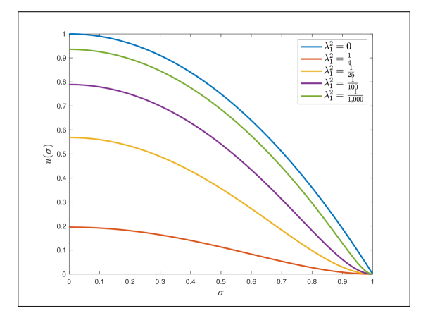
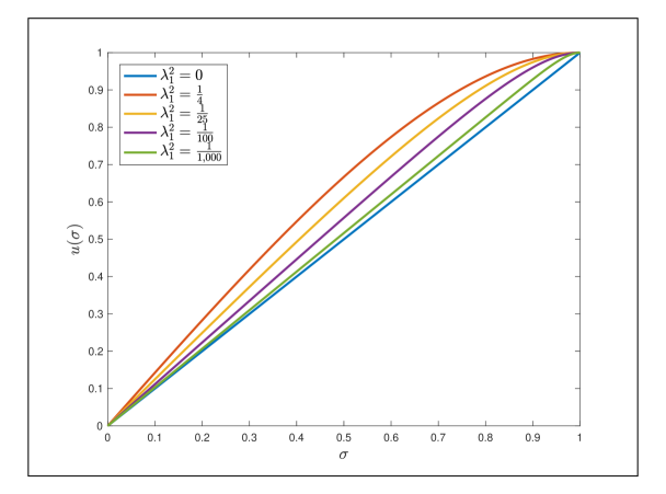
Motivated by Figure 1, we will now show pointwise convergence of (4.22) to the classical Navier-Stokes solution, . Clearly, so we will consider . The argument for is similar. We will use the following large asymptotics for [1]:
We then can conclude that
From the above calculation, we see that
proving pointwise convergence to the classical solution.
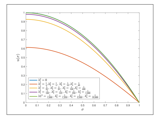
We now consider setting of weak adherence boundary conditions. Recall our nondimensionalized solution in the weak adherence setting:
| (4.23) |
Motivated by Figure 2, we will now show pointwise convergence of (4.23) to the classical Navier-Stokes solution, . Clearly, , so we show pointwise convergence to the classical solution for . The case follows a similar argument. We use the same asymptotics for as above in addition to the following for the second derivative:
Using these asymptotics, we see that
and
We note that by (2.44), We then conclude that
as . We have thus shown
proving the pointwise convergence of to the classical solution in the weak adherence case.
Via very similar arguments, one may also show that the dimensionless discharge rate converges to the classical dimensionless rate as for both strong adherence and weak adherence boundary conditions; the details are left to the interested reader.
5. Taylor-Couette Flow
We now consider rotational flow for a tube with an outer radius rotating with angular velocity . The velocity and pressure are taken to be of the form
| (5.1) |
Then
| (5.2) | ||||
| (5.3) | ||||
| (5.4) |
5.1. General solution
The -component of (2.50) for reads
| (5.5) |
where . The above equation has the following general solution:
| (5.6) |
with constants and determined by the boundary conditions. We require to be regular at the origin and thus, . We now determine the solutions satisfying either strong adherence or weak adherence boundary conditions.
5.2. Strong adherence boundary conditions
The boundary condition is equivalent to the requirement that . Thus, the strong adherence boundary conditions are as follows:
It is readily checked that the solutions are
so the solution can be written as
The dimensionless velocity as a function of is given by
| (5.7) |
where .
5.3. Weak adherence boundary conditions
For the weak adherence case, we assume that . Since we assume that , weak adherence requires that
| (5.8) |
We observe that the classical solution satisfies and (5.8) does not, and thus, the velocity profile satisfying weak adherence conditions is
The nondimensionalized solution is then given by
| (5.9) |
5.4. Convergence to the solution for the classical Navier-Stokes model
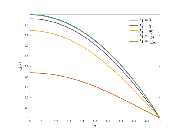
Motivated by Figure 5, we now prove pointwise convergence of the dimensionless velocity field given by (5.7) to the dimensionless velocity field corresponding to the classical Navier-Stokes model, .
Clearly and , so, we only consider . We use the asymptotics for [1]:
| (5.10) |
as . Then for ,
| (5.11) | ||||
| (5.12) | ||||
| (5.13) | ||||
| (5.14) |
We conclude that for each ,
| (5.15) | |||
| (5.16) |
Thus, for all ,
| (5.17) |
as , proving pointwise convergence to the solution for the classical Navier-Stokes model. Since the classical solution and the weak adherence solution are the same, there is no convergence to show for weak adherence boundary conditions.
5.5. The pressure
The -component for Taylor-Couette flow determines the pressure, which we assume is regular and satisfies . The pressure satisfies the following differential equation:
| (5.18) |
where is the velocity. Carrying out the differentiation, we see that satisfies
| (5.19) |
We will label the right-hand side as . Using the change of variables , we have that the ODE that satisfies is
| (5.20) |
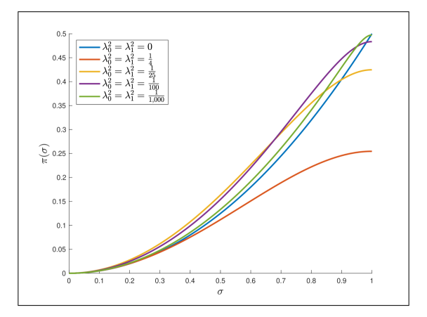
The solution to this ODE is given as the following via variation of parameters:
Thus,
With , the dimensionless pressure with then satisfies
| (5.21) | ||||
| (5.22) |
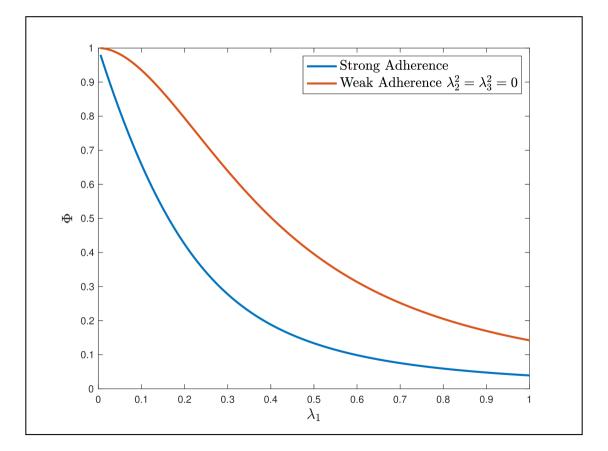
As shown in Figure 6, the dimensionless pressure field approaches the classical solution. A comprehensive theory establishing convergence of both the nondimensional velocity and pressure fields to their classical limits will be pursued elsewhere.
References
- [1] M. Abramowitz and I. A. Stegun. Handbook of Mathematical Functions with Formulas, Graphs, and Mathematical Tables, volume 55 of National Bureau of Standards Applied Mathematics Series. U.S. Government Printing Office, Washington, D.C., 1964.
- [2] H. Askes and E. C. Aifantis. Gradient elasticity in statics and dynamics: An overview of formulations, length scale identification procedures, finite element implementations and new results. Int. J. Solids Struct., 48(13):1962–1990, 2011.
- [3] S. Bair, M. Khonsari, and W. O. Winer. High-pressure rheology of lubricants and limitations of the Reynolds equation. Tribology Int., 31:573–586, 1998.
- [4] C. Barus. Isotherms, isopiestics and isometrics relative to viscosity. Am. J. Sci., 45:87–96, 1893.
- [5] G. Bayada, B. Cid, G. García, and C. Vázquez. A new more consistent Reynolds model for piezoviscous hydrodynamic lubrication problems in line contact devices. Appl. Math. Model., 37:8505–8517, 2013.
- [6] Albrecht Bertram and Samuel Forest, editors. Mechanics of Strain Gradient Materials. Springer International Publishing, Cham, 2020.
- [7] P. W. Bridgman. The effect of pressure on the viscosity of forty-four pure liquids. Proc. Am. Acad. Art. Sci., 61:57–99, 1926.
- [8] P. W. Bridgman. The Physics of High Pressure. MacMillan, 1931.
- [9] B. J. Chung and A. Vaidya. On the slow motion of a sphere in fluids with non-constant viscosities. Int. J. Eng. Sci., 48(1):78–100, 2010.
- [10] E. Cosserat and F. Cosserat. Theorie des Corps Deformables. Hermann, Paris, 1909.
- [11] M. Degiovanni, A. Marzocchi, and S. Mastaglio. Existence, Uniqueness, and Regularity for the Second–Gradient Navier–Stokes Equations in Exterior Domains. In T. Bodnár, G. P. Galdi, and Š. Nečasová, editors, Waves in Flows, pages 181–202. Springer International Publishing, Cham, 2021. Series Title: Advances in Mathematical Fluid Mechanics.
- [12] F. Dell’Isola, U. Andreaus, and L. Placidi. At the origins and in the vanguard of peridynamics, non-local and higher-gradient continuum mechanics: an underestimated and still topical contribution of Gabrio Piola. Math. Mech. Solids, 20(8):887–928, 2015.
- [13] F. Dell’Isola, A. Della Corte, and I. Giorgio. Higher-gradient continua: the legacy of Piola, Mindlin, Sedov and Toupin and some future research perspectives. Math. Mech. Solids, 22(4):852–872, 2017.
- [14] F. Dell’Isola, P. Seppecher, and A. Della Corte. Higher gradient theories and their foundations. Encyclopedia of Continuum Mechanics, pages 1090–1099, 2020.
- [15] M. M. Denn. Pressure drop-flow rate equation for adiabatic capillary flow with a pressure- and temperature-dependent viscosity. Polym. Eng. Sci., 21:65–68, 1981.
- [16] E. Fried and M. E. Gurtin. Tractions, balances, and boundary conditions for nonsimple materials with application to liquid flow at small-length scales. Arch. Ration. Mech. Anal., 182(3):513–554, 2006.
- [17] E. Fried and M. E. Gurtin. A continuum mechanical theory for turbulence: a generalized Navier–Stokes- equation with boundary conditions. Theor. Comput. Fluid Dyn., 22(6):433–470, November 2008.
- [18] F. Gazzola and P. Secchi. Some results about stationary Navier-Stokes equations with a pressure-dependent viscosity. In Proceedings of the International Conference on Navier-Stokes Equations: Theory and Numerical Methods, volume 388 of Pitman Research Notes in Mathematics, pages 31–37. Longman, Varenna, 1998.
- [19] P. Germain. La méthode des puissances virtuelles en mécanique des milieux continus. I. Théorie du second gradient. J. Mécanique, 12:235–274, 1973.
- [20] P. Germain. The method of virtual power in continuum mechanics. part 2: Microstructure. SIAM J. Appl. Math., 25(3):556–575, 1973.
- [21] G. Giantesio, A. Girelli, C. Lonati, A. Marzocchi, A. Musesti, and B. Straughan. Thermal convection in a higher velocity gradient and higher temperature gradient fluid, 2024. arXiv:2405.04155.
- [22] G. G. Giusteri and E. Fried. Slender-body theory for viscous flow via dimensional reduction and hyperviscous regularization. Meccanica, 49(9):2153–2167, September 2014.
- [23] G. G. Giusteri, A. Marzocchi, and A. Musesti. Three-dimensional nonsimple viscous liquids dragged by one-dimensional immersed bodies. Mech. Res. Commun., 37(7):642–646, October 2010.
- [24] G. G. Giusteri, A. Marzocchi, and A. Musesti. Nonsimple isotropic incompressible linear fluids surrounding one-dimensional structures. Acta Mech, 217(3-4):191–204, March 2011.
- [25] A. E. Green and R. S. Rivlin. Multipolar continuum mechanics. Arch. Rational Mech. Anal., 17:113–147, 1964.
- [26] A. E. Green and R. S. Rivlin. Simple force and stress multipoles. Arch. Rational Mech. Anal., 16:325–353, 1964.
- [27] T. Gustafsson, K. R. Rajagopal, R. Stenberg, and J. Videman. Nonlinear Reynolds equation for hydrodynamic lubrication. Appl. Math. Model., 39:5299–5309, 2015.
- [28] D. R. Gwynllyw, A. R. Davies, and T. N. Phillips. On the effects of a piezoviscous lubricant on the dynamics of a journal bearing. J. Rheol., 40:1239–1266, 1996.
- [29] K. D. Housiadas, G. C. Georgiou, and R. I. Tanner. A note on the unbounded creeping flow past a sphere for Newtonian fluids with pressure-dependent viscosity. Int. J. Eng. Sci., 86:1–9, 2015.
- [30] J. Hron, J. Málek, J. Nečas, and K. R. Rajagopal. Numerical simulations and global existence of solutions of two-dimensional flows of fluids with pressure- and shear-dependent viscosities. Math. Comput. Simul., 61(3–6):297–315, 2003.
- [31] J. Hron, J. Málek, and K. R. Rajagopal. Simple flows of fluids with pressure-dependent viscosities. Proc. R. Soc. Lond., Ser. A, Math. Phys. Eng. Sci., 457:1603–1622, 2001.
- [32] A. Janečka and V. Průša. The motion of a piezoviscous fluid under a surface load. Int. J. Non-Linear Mech., 60:23–32, 2014.
- [33] A. Kalogirou, S. Poyiadji, and G. C. Georgiou. Incompressible Poiseuille flows of Newtonian liquids with a pressure-dependent viscosity. J. Non-Newtonian Fluid Mech., 166:413–419, 2011.
- [34] S. Knauf, S. Frei, T. Richter, and R. Rannacher. Towards a complete numerical description of lubricant film dynamics in ball bearings. Comput. Mech., 2013.
- [35] J. Koplik and J. R. Banavar. Continuum deductions from molecular hydrodynamics. Annu. Rev. Fluid Mech., 27:257–292, 1995.
- [36] J. Koplik, J. R. Banavar, and J. F. Willemsen. Molecular dynamics of pioseuille flow and moving contact lines. Phys. Rev. Lett., 60:1282–1285, 1988.
- [37] A. Krawietz. Surface tension and reaction stresses of a linear incompressible second gradient fluid. Contin. Mech. Thermodyn., 34(4):1027–1050, 2022.
- [38] E. Marušić-Paloka and I. Pažanin. A note on the pipe flow with a pressure-dependent viscosity. J. Non-Newtonian Fluid Mech., 197:5–10, 2013.
- [39] G. A. Maugin. Non-classical Continuum Mechanics, volume 51 of Advanced Structured Materials. Springer, Singapore, 2017.
- [40] Gérard A. Maugin. A historical perspective of generalized continuum mechanics. In Holm Altenbach, Vladimir I. Erofeev, and Gérard A. Maugin, editors, Mechanics of Generalized Continua: From the Micromechanical Basics to Engineering Applications, pages 3–19. Springer, Berlin, 2011.
- [41] Gérard A. Maugin. Generalized continuum mechanics: Various paths. In Continuum Mechanics Through the Twentieth Century: A Concise Historical Perspective, pages 223–241. Springer, Dordrecht, 2013.
- [42] X.-B. Mi and A. T. Chwang. Molecular dynamics simulations of nanochannel flows at low reynolds numbers. Molecules, 8:193–206, 2003.
- [43] R. D. Mindlin. Micro-structure in linear elasticity. Arch. Rational Mech. Anal., 16:51–78, 1964.
- [44] R. D. Mindlin. Second gradient of strain and surface-tension in linear elasticity. Int. J. Solids Struct., 1(4):417–438, 1965.
- [45] R. D. Mindlin and N. N. Eshel. On first strain-gradient theories in linear elasticity. Int. J. Solids Struct., 4(1):109–124, 1968.
- [46] A. Musesti. Isotropic linear constitutive relations for nonsimple fluids. Acta Mech., 204:81–88, 2009.
- [47] NobelPrize.org. Percy W. Bridgman–Facts, 2024. Nobel Prize Outreach AB.
- [48] H. Okamura and D. M. Heyes. Comparisons between molecular dynamics and hydrodynamics treatment of nonstationary thermal processes in a liquid. Phys. Rev. E., 70:061206, 2004.
- [49] G. Piola. Memoria intorno alle equazioni fondamentali del movimento di corpi qualsivogliono considerati secondo la naturale loro forma e costituzione. Modena, Italy: B. D. Camera, 1846.
- [50] V. Průša. Revisiting Stokes first and second problems for fluids with pressure-dependent viscosities. Int. J. Eng. Sci., 48(12):2054–2065, 2010.
- [51] K. R. Rajagopal. Remarks on the notion of “pressure”. Int. J. Non-Linear Mech, 71:165–172, 2015.
- [52] K. R. Rajagopal, G. Saccomandi, and L. Vergori. Flow of fluids with pressure- and shear-dependent viscosity down an inclined plane. J. Fluid Mech., 706:173–189, 2012.
- [53] K. R. Rajagopal, G. Saccomandi, and L. Vergori. Unsteady flows of fluids with pressure dependent viscosity. J. Math. Anal. Appl., 404:362–372, 2013.
- [54] K. R. Rajagopal and A. Z. Szeri. On an inconsistency in the derivation of the equations of elastohydrodynamic lubrication. Proc. R. Soc. Lond., Ser. A, Math. Phys. Eng. Sci., 459:2771–2786, 2003.
- [55] M. Rehor and V. Průša. Squeeze flow of a piezoviscous fluid. Appl. Math. Comput., 274:414–429, 2016.
- [56] M. Renardy. Some remarks on the Navier-Stokes equations with a pressure-dependent viscosity. Commun. Partial Differ. Equ., 11:779–793, 1986.
- [57] D. J. Steigmann, M. Bîrsan, and M. Shirani. Lecture Notes on the Theory of Plates and Shells: Classical and Modern Developments, volume 274. Springer Nature, 2023.
- [58] B. Straughan. Thermal convection in a higher-gradient Navier–Stokes fluid. Eur. Phys. J. Plus, 138(1):60, January 2023.
- [59] R. A. Toupin. Elastic materials with couple-stresses. Arch. Rational Mech. Anal., 11:385–414, 1962.
- [60] R. A. Toupin. Theories of elasticity with couple-stress. Arch. Rational Mech. Anal., 17:85–112, 1964.
- [61] K. P. Travis and K. E. Gubbins. Poiseuille flow of Lennard-Jones fluids in narrow slit pores. J. Chem. Phys., 112:1984–1994, 2000.
- [62] K. P. Travis, B. D. Todd, and D. J. Evans. Departure from Navier-Stokes hydrodynamics in confined fluids. Phys. Rev. E, 55:4288–4295, 1997.
- [63] M. Vasudevaiah and K. R. Rajagopal. On fully developed flows of fluids with a pressure dependent viscosity in a pipe. Appl. Math., 50:341–353, 2005.
C. Balitactac
Department of Mathematics, University of North Carolina
Chapel Hill, NC 27599, USA
C. Rodriguez
Department of Mathematics, University of North Carolina
Chapel Hill, NC 27599, USA