The HOSTS Survey: Suspected variable dust emission and constraints on companions around $\theta$ Boo

Abstract

Context. During the Hunt for Observable Signatures of Terrestrial Systems (HOSTS) survey by the Large Binocular Telescope Interferometer (LBTI), an excess emission from the main sequence star $\theta$ Boo (F7V spectral type, 14.5 pc distance) was observed. This excess indicates the presence of exozodiacal dust near the habitable zone (HZ) of the star. Previous observations from Spitzer and Herschel showed no sign of outer cold dust within their respective detection limits. Since exozodiacal dust is generally thought to originate from material located further out in the system, the source of exozodiacal dust around $\theta$ Boo remains unclear.

Aims. Additional nulling and high-contrast adaptive optics (AO) observations were taken to spatially constrain the dust distribution, search for variability, and directly image potential companions in the system. This study presents the results of these observations and provides an interpretation of the inner system’s architecture.

Methods. The star was observed using the LBTI’s N’-band nulling mode during three epochs in 2017, 2018, and 2023. The dust distribution is modeled and constrained for each epoch using the standard LBTI nulling pipeline, assuming a vertically thin disk with a face-on inclination. In addition, high-contrast AO observations are performed in the L’-band and H-band to constrain the presence of substellar companions around the star.

Results. Several solutions are found for the dust distribution, and for each epoch. However, the LBTI nulling observations are not able to discriminate between them. Using the upper limits from previous observations, we constrain the representative size of the dust grains around 3-5 µm. A tentative increase in dust brightness is also measured at the Earth-equivalent insolation distance between 2017 and 2023. This increase corresponds to the injection of $4\times 10^{-8}-4\times 10^{-7}\,M_{\oplus}$ new material in the disk. Several options are considered to explain the origin of the observed dust and its variability, but no clear sources could be identified from the current observations. Partly because our high-contrast AO observations could only constrain the presence of companions down to $11\,M_{\text{Jup}}$ at 1.3″separation.

1 Introduction

Direct imaging of exoplanets is a challenging type of observation in modern astronomy due to the high star-planet contrast and their small angular separation. Even if only $\sim$1 % of currently known exoplanets have been directly imaged, these observations permit detailed characterization of their atmospheres. Present or expected improvements in high-angular resolution capabilities, from 30 m-class telescopes (Quanz et al., 2015; Bowens et al., 2021) and interferometry (ground-based: Defrère et al. 2018; Wagner et al. 2021a, 2021b; Ertel et al. 2022; or space-based: Kammerer et al. 2022), are opening up the Habitable Zone (HZ) of nearby main-sequence stars for direct imaging. The HZ commonly refers to the circumstellar region where planetary surfaces may sustain liquid water given an adequate atmosphere (Kopparapu et al., 2013). This region is relevant for the search of potential exoplanets located at the Earth-equivalent insolation distance (EEID) – the orbital distance where objects get the same irradiance as Earth – and the assessment of their habitability. However, this region can also be rich in debris material, similar to the zodiacal cloud of the Solar System, called “exozodiacal dust”. Like other debris disks found at larger separation, exozodiacal disks are expected to appear around the end of planetary formation, during the disk clearing phase (between 10 Myr and a few Gyr age, Hinz et al., 2009; Ercolano & Pascucci, 2017). Collisions and evaporation of planetesimals serve as a source for exozodiacal dust (Kennedy & Piette, 2015; Marboeuf et al., 2016; Faramaz et al., 2017; Rigley & Wyatt, 2022) while other phenomena tend to deplete it (e.g. Poynting-Robertson (P-R) drag: Wyatt & Whipple 1950; Burns et al. 1979; planetary sweeping: Bonsor et al. 2018; or radiation pressure: Burns et al. 1979). The study of exozodiacal disks around nearby main-sequence stars has several main purposes: (1) to study the properties and dynamics of the dust (Mennesson et al., 2014; Defrère et al., 2015; Lebreton et al., 2016); (2) to give insights into the architecture and formation mechanisms of planetary systems (Stark & Kuchner, 2008); and (3) to evaluate the cometary bombardment and its impact on the habitability of inner planetary systems (Chyba et al., 1990; O’Brien et al., 2014; Rotelli et al., 2016; Kral et al., 2018; Wyatt et al., 2020; Ritson et al., 2020). Its study is also important to estimate the impact of these disks on rocky planet imaging, from the shot noise they generate in the infrared (Defrère et al., 2010; Stark et al., 2014, 2019), and from their scattering of the stellar light in the visible (Beichman et al., 2006; Defrère et al., 2012; Roberge et al., 2012).

A survey of exozodiacal disks was carried out by the Hunt for Observable Signatures of Terrestrial Systems (HOSTS) survey (Ertel et al., 2018, 2020) which quantified the presence of warm dust ($\sim$300 K, i.e., located in the HZ) and its surface density around nearby ($<$30 pc) main-sequence stars. The survey was performed with the nulling mode of the Large Binocular Telescope Interferometer (LBTI: Defrère et al., 2015; Hinz et al., 2016; Ertel et al., 2020). As part of the survey, the F7V type star $\theta$ Boo was observed. This star, located at 14.5 pc, showed signs of HZ dust emission estimated at $148.2\pm 27.7$ zodi (1 zodi being the dust surface density at the EEID of the Solar System, i.e., 1 au; see definition in Weinberger et al., 2015; Kennedy et al., 2015). Table 1 gives a summary of the stellar parameters of $\theta$ Boo that are used in this study. Among these parameters, the stellar luminosity L_⋆ is used to calculate the local EEID using the method presented in Weinberger et al. (2015), where the radius $r_{\text{EEID}}$ is proportional to $\sqrt{\text{L}_{\star}}$. In the case of $\theta$ Boo, we find $r_{\text{EEID}}\simeq 2\,au$, which corresponds to a separation of $\sim 138$ mas. The star was previously observed by the space telescopes Spitzer (2004) and Herschel (2010) at 24, 70, and 100 µm wavelength to look for warm ($\sim$600 K) and cold dust ($\sim$120 K) emissions. These surveys showed no significant emission excess within their detection limits (Bryden et al., 2006; Trilling et al., 2008; Gáspár et al., 2013; Montesinos et al., 2016). Figure 1 represents the observed spectral energy distribution (SED) of $\theta$ Boo, and the upper limits for the dust emission obtained from space surveys. The upper limits are estimated following the method used in Yelverton et al. (2019), where the observed data are fitted by a model with both a stellar and a dust component. The stellar component is a PHOENIX BT-Settl model (Allard et al., 2012), and the dust component is a modified blackbody. The error bars of the observed data are then propagated on the results of the dust model.

Table 1: Relevant stellar parameters for $\theta$ Boo used in this study.

Parameter	Value	Reference
Distance d [pc]	14.5$\pm$0.04	(1)
T${}_{\text{eff}}$ [K]	6315$\pm$10	(2)
Age [Myr]	500$\pm$250	(3)
L⋆ [L⊙]	4.01$\pm$0.02	(4)
M⋆ [M⊙]	1.31$\pm$0.07	(4)
R⋆ [R⊙]	1.73$\pm$0.01	(4)
($B-V$)	0.50	(5)
$\nu\sin(i)$ [km/s]	31.8$\pm$2	(6)
$\log R^{\prime}_{\text{HK}}$	-4.5$\pm$0.1	(7)

Notes. T${}_{\text{eff}}$ is the effective temperature, L_⋆ the luminosity, M_⋆ the mass, R_⋆ the radius, and $\nu\sin(i)$ the projected rotational velocity. $R^{\prime}_{\text{HK}}$ is an activity indicator defined as $F^{\prime}_{\text{HK}}/\sigma T^{4}_{\text{eff}}$ with $F^{\prime}_{\text{HK}}$ being the chromospheric flux in the H and K lines of Ca II. The estimated age of the star is however uncertain as it depends on the method used (see discussion in Sec. 4).
References. (1) Gaia Collaboration et al. (2016, 2023); (2) Montesinos et al. (2016); (3) Gáspár et al. (2013); (4) Boyajian et al. (2013); Johnson et al. (1966); (6) Rachford & Foight (2009); (7) Pace (2013)

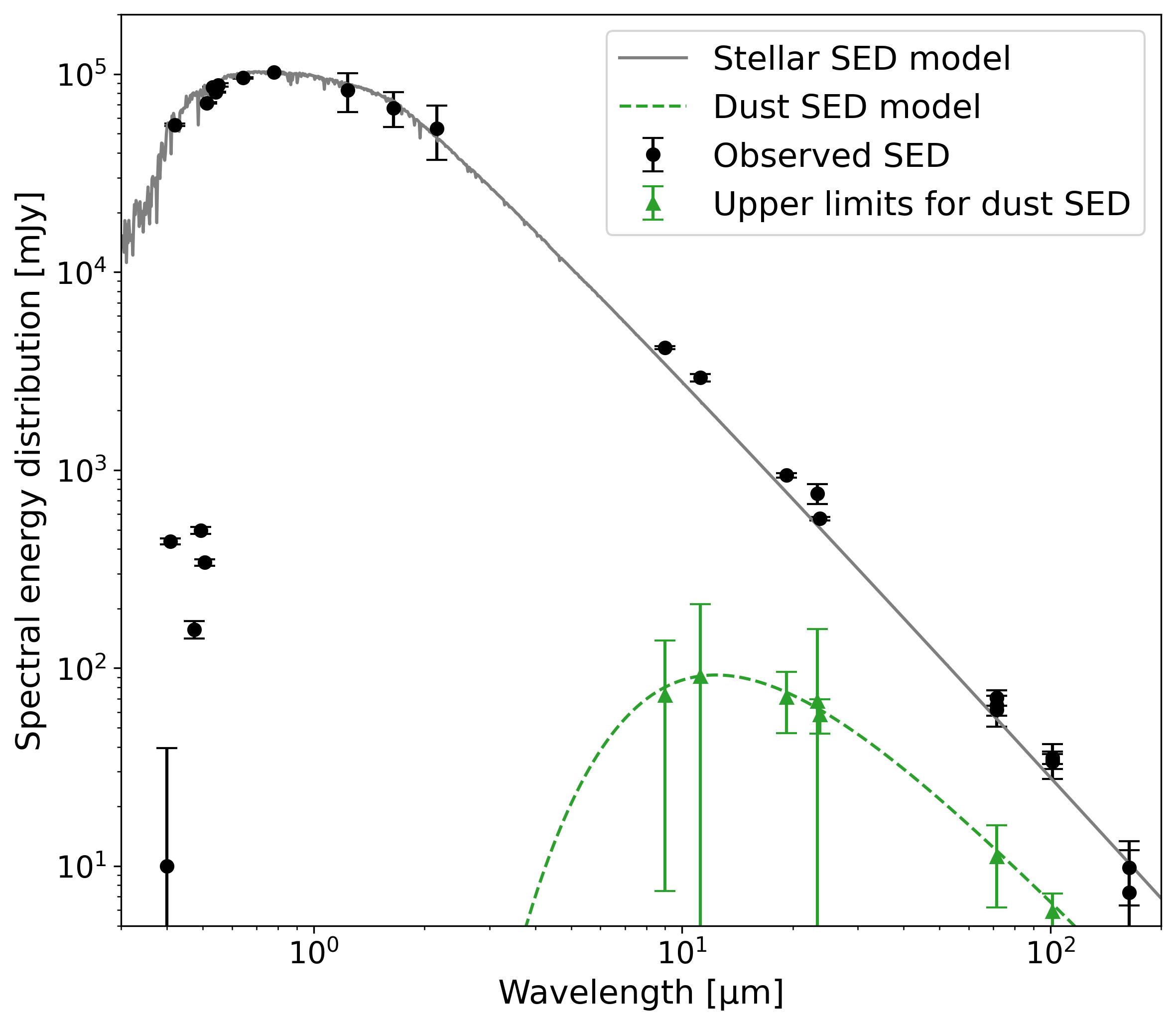
Figure 1: Observed spectral energy distribution (SED) of $\theta$ Boo. The figure indicates the observed photometric data (black points), with the best fit stellar model (gray line), and dust model (green dashed line). The green points are the upper limits of the dust emission.

This raises the question of the origin of the exozodiacal dust in the system. The presence of such warm dust is found to be strongly correlated with the presence of a cold debris disk (Ertel et al., 2020). This is supported by the statistical results of the HOSTS survey which found a detection rate of HZ dust of $78^{+8}_{-18}$ % in systems with a known cold debris disk. Only 3 of 28 stars have known HZ dust without cold debris ($\theta$ Boo being one of them). To investigate the nature of the exozodiacal disk of $\theta$ Boo, a new observation in nulling mode was performed by the LBTI in 2023 with a wider range of parallactic angles than the observations done during the HOSTS survey. This work is part of an effort to study individual targets of the HOSTS survey ($\beta$ Leo: Defrère et al. 2021; $\alpha$ Lyr: Faramaz et al. in prep.; 110 Her: Rousseau et al. in prep.; $\epsilon$ Eri: Weinberger et al. in prep.; $\beta$ Uma: Bryden et al. in prep.), and investigate the nature of these disks.

In this paper, a descriptive model for the dust spatial distribution is proposed for $\theta$ Boo. The presence of companions is also constrained using observations from the LBTI/L- and M-band InfraRed Camera (LMIRCam) and System for coronagraphy with High-order Adaptive optics from R to K-band (SHARK)-Near InfraRed (NIR) at the Large Binocular Telescope (LBT). Section 2 describes the different observations of $\theta$ Boo used in this study. Section 3 explains the different data reduction processes for these observations and their results. The constraints on the presence of possible companions in the system are presented in Sec 4. The models of the dust distribution and its variability at the EEID are then shown in Sec 5. We finally discuss the constraints on the dust distribution, its possible origins, and the source of its variability in Sec. 6.

2 Observations of $\theta$ Boo

2.1 Instrument description

The nulling observations of $\theta$ Boo were carried out at the LBT on UT 2017 April 11 and UT 2018 May 23 with the LBTI/Nulling Optimized Mid-Infrared Camera (NOMIC) in the N’-band (9.81-12.41 µm) in the context of the HOSTS survey. A new nulling observation with NOMIC was acquired on UT 2023 May 25. Finally, high-contrast adaptive optics (AO) imaging with LMIRCam in the L’-band (3.41-3.99 µm) and with SHARK-NIR in the H-band (1.38 to 1.82 µm) were acquired on UT 2024 February 24. Table 2 gives an overview of these observations.

Table 2: Overview of the $\theta$ Boo observations.

Night [UT]	Spectral Band	Instrument	Observing mode	Time [UT]	PA [deg]
2017-04-11	N’	LBTI/NOMIC	Nulling	07:51-09:06	(-159,+155)
2018-05-23	N’	LBTI/NOMIC	Nulling	05:05-05:43	(-157,+179)
2023-05-25	N’	LBTI/NOMIC	Nulling	03:58-07:35	(-128,+119)
2024-02-24	L’	LBTI/LMIRCam	Imaging	10:18-01:55	(-140,+116)
2024-02-24	H	LBT/SHARK-NIR	Imaging	10:18-01:55	(-140,+116)

Notes. UT stands for Universal Time, PA stands for parallactic angle.

Hill et al. (2012) present the LBT which consists of two 8.4 m diameter apertures, each corrected with AO. AO ensure a Strehl ratio of 80%, 95%, and 99% at 1.6 µm, 3.8 µm, and 10 µm respectively using Pyramid Wave Front Sensing (WFS) with the visible part of the light Bailey et al. (2010, 2014); Pinna et al. (2016). The infrared part of the light is directed towards the Nulling and Imaging Camera (NIC) where it is split and focused on the different cameras as explained in Hinz et al. (2008).

The LBTI corresponds to the instrument that combines the light from the two LBT apertures to perform interferometric observations (Hinz et al., 2016). LMIRCam and the NOMIC can be used in this configuration by imaging both beams separately or by overlapping them. Figure 2 gives an overview of the architecture of the LBTI. A K-band fast readout camera called Phasecam monitors the phase difference between the two apertures (Defrère et al., 2014). It allows to sense the differential piston between the two LBT apertures, and to fix it by using two piston correctors located upstream on the tip-tilt mirrors.

The SHARK-NIR is located near the Gregorian focus of the left aperture and performs observations in the near-infrared (Farinato et al., 2022; Marafatto et al., 2022). LMIRCam can observe from J- to M-bands and NOMIC in the N-band.

The only relevant change made at the LBT between the first observations of 2017/2018 and 2024 is the AO upgrade (Pinna et al., 2016). This upgrade is not expected to have a major impact on the nulling observations as the previous AO system already achieved a similar Strehl ratio in the N-band on the HOSTS targets. Moreover, any change of AO performance would have resulted in changes in instrumental null or phase jitter, which are considered in the data reduction pipeline and the error estimations.

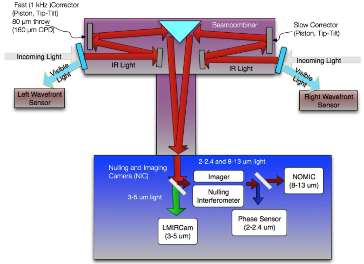
Figure 2: Block diagram of the LBTI architecture with light from the two apertures arriving at top left and right, and the beam combiner subsystem (in purple) and the NIC cryostat (in blue). Both the beam combiner and the NIC are maintained at cryo-temperatures. At the entrance of the beam combiner subsystem, the visible light is reflected by dichroics and directed to the WFS units. Infrared light is transmitted to the beam combiner where two mirrors adjust the tip/tilt and the OPD of the beams for the nulling interferometry mode. After recombination of the two LBTI’s pupils by the roof mirror, the light is split in the NIC. The L-band (3-5 µm) is directed to LMIRCam for high-contrast imaging of exoplanets whereas the K-band (1.5-2.5 µm) is directed to the Phasecam to monitor the differential tip/tilt and phase between the two apertures. Finally, the N-band (8-13 µm) light is directed to NOMIC which can be used either in imaging interferometry or nulling interferometry modes.

2.2 N’-band imaging observations

In the N’-band, the NOMIC camera was used in a configuration that can perform nulling observations. In this configuration, the phase difference between the two apertures is locked at $\pi$. When combined in the pupil plane, light from a point source at the center of the field of view (FOV) will destructively interfere and not be observed when re-imaged at the detector plane. However, off-axis sources add an extra phase difference between the apertures depending on their on-sky position. This means that emission from off-axis sources and from any sufficiently extended parts of the star (called “stellar leakage” or “instrumental null depth”) are imaged on the NOMIC camera.

The throughput of off-axis sources on the camera with regards to their on-sky position is called the “transmission map” $T$. In the case of the LBTI, which consists of two apertures separated by a baseline $B=$14.4 m, $T=\sin^{2}(\pi\phi B/\lambda)$ with $\phi$ being the on-sky position projected on the baseline vector, and $\lambda$ the wavelength (Kennedy et al., 2015). The transmission of an object on the camera thus depends on its on-sky position but also on the parallactic angle rotation during the night (i.e., the baseline rotation). The coherent FOV $\theta_{c}$ – which corresponds to the on-sky region where light sources can interfere – is given by

$$\theta_{c}\equiv\frac{\lambda^{2}}{B\times\Delta\lambda},$$ (1)

with $\Delta\lambda$ the spectral bandwidth (Thompson et al., 1986). In the case of nulling in the N’-band (9.81-12.41 µm), we have a coherent FOV $\theta_{c}\simeq 670$ mas.

The amount of instrumental null depth can be estimated by using a set of calibrator stars “CAL” before and after the different observations of the science target $\theta$ Boo. Those calibrators were selected following Mennesson et al. (2014) using the two catalogs Bordé et al. (2002) and Mérand et al. (2005), with additional stars from the JSDC catalog and the SearchCal tool from Chelli et al. (2016). The calibrators used in this study and their properties are listed in Table 3.

Observations consist of several observation blocks (OBs), with each corresponding to series of 2000$\times$42.7 ms frames. Between each nulling OB, the telescope is offset by $\pm$2.3 ″at the detector in an up/down nod movement. The instrument uses an Aquarius detector, with a FOV of 18″$\times$18″, and a pixel scale of 17.9 mas. This allows the mid-infrared thermal background noise located at pixels which may have received any signal in the previous observation to be measured. Each observation then has several nulling OBs (where the two beams are overlapping), one photometric OB (where the two beams are separated on the camera), and one background OB (where the beams are nodded off the detector). The N’-band observations on 2017 April 11, 2018 May 23, and 2023 May 25 aimed at imaging the exozodiacal dust at a separation range of 40-700 mas (i.e., 0.6-10.4 au for $\theta$ Boo). Table 2 gives a summary for the three observing nights. For each night, the sequence of observations is: CAL1-$\theta$ Boo-CAL2 (2017 April 11); CAL1-$\theta$ Boo-CAL3 (2018 May 23); and CAL1-$\theta$ Boo-CAL4-$\theta$ Boo-CAL5 (2023 May 25). Every observation uses CAL1 at the beginning, which allows to compare the results between the different nights.

Table 3: Basic properties of $\theta$ Boo and its calibrators for the 2017 April 11, 2018 May 23 and 2023 May 25 nulling observations

ID	HD	R.A.	Dec.	Spectral Type	$m_{V}$	$m_{K}$	$\theta_{LD}$$\pm$1$\sigma$ [mas]	References
$\theta$ Boo	126660	14 25 11.8	+51 51 02.7	F7V	4.04$\pm$0.002	2.80$\pm$0.09	1.14$\pm$0.05	[Du02], [Kh09]
CAL 1	128902	14 38 12.6	+43 38 31.7	K4III	5.72$\pm$0.004	2.32$\pm$0.259	1.83$\pm$0.25	[Kh09]
CAL 2	138265	15 27 51.4	+60 40 12.8	K5III	5.91$\pm$0.004	1.59$\pm$0.238	2.83$\pm$0.35	[Kh09]
CAL 3	131507	14 51 26.4	+59 17 38.4	K4III	5.48$\pm$0.003	2.21$\pm$0.233	1.97$\pm$0.24	[Kh09]
CAL 4	128000	14 32 30.9	+55 23 52.8	K5III	5.72$\pm$0.004	2.14$\pm$0.195	2.1$\pm$0.21	[Kh09]
CAL 5	138265	15 27 51.4	+60 40 12.8	K5III	5.91$\pm$0.004	1.59$\pm$0.238	2.83$\pm$0.35	[Kh09]

References. Coordinates and spectral types from SIMBAD; V&K magnitudes and error bars from [Du02] Ducati (2002) and [Kh09] Kharchenko & Roeser (2009); Limb-darkened angular diameters and their 1$\sigma$ uncertainties from Chelli et al. (2016).

2.3 L’-band imaging observations

Observations with LMIRCam were taken on the LBT right arm (with one 8.4 m aperture) using Director’s Discretionary Time (DDT). The L’-band observations obtained on 2024 February 24 aimed at imaging a potential companion at a separation range of 0.3-4″ (i.e., 4-58 au for $\theta$ Boo, see Sec. 3.2). They consisted of 28 sequences of exposures, each with 2000 images of 55 ms integration time. The total integration time was then 3080 s ($\sim$51 minutes). No coronograph was used. The centering was done using a rotational based algorithm following Morzinski et al. (2015). The detector is a Teledyne H2RG with a FOV of 20″$\times$20″, and a pixel scale of 10.9 mas. The observations were taken in pupil-stabilized mode allowing the rotation of the FOV to perform angular differential imaging (ADI: Marois et al., 2006). During the observation, the parallactic angle changed by 104$\degree$ and the seeing fluctuated between 1.05″ and 2″. To monitor the thermal sky background and the detector drifts, the image of the star was nodded up and down on the detector by an offset angle of 4.5″ between every observing block.

2.4 NIR imaging observations

In parallel with LMIRCam, observations with SHARK-NIR operating on the LBT left arm were also taken. The observations were performed exploiting the broadband H filter (central wavelength at 1.6 µm and bandwidth of 0.218 µm) and the Gaussian Lyot coronagraph with an inner working angle (IWA) of 150 mas. The detector is a Teledyne H2RG with a FOV of 18$\arcsec\times$18$\arcsec$, and a pixel scale of 14.5 mas per pixel. To avoid detector saturation near the star and to minimize exposure time, we selected an observing mode where only a central region of dimensions 2048 x 200 pixels were read out. Therefore the usable region for the detection of possible companions and for the definition of the contrast is limited to a separation of 1.3″ (see Sec. 3.3). The exposure time for each frame was 0.84 s while the total number of frames acquired was 6855. This gave a total exposure time of 5758.2 s ($\sim$96 minutes) on the target. The observations were also taken to allow ADI during the post-processing. To correctly estimate the obtained contrast, images of the stellar point spread function (PSF) without the coronagraph were taken at the beginning and at the end of the observations. These frames were taken using an appropriate neutral density filter (ND3) to avoid detector saturation.

3 Data reduction

3.1 N’-band nulling data

The LBTI nulling pipeline from Defrère et al. (2016) is used for the N’-band nulling data reduction and calibration. In a nutshell, the pipeline first corrects the raw images by removing bad pixels and subtracting the mid-infrared thermal background. As the background cannot be measured at the star position when the star is present, it is estimated from the series of OBs with an opposite nod position. This way, the background can be subtracted using either the mean value of the series or a Principle Component Analysis (PCA) approach Rousseau et al. (2024). This work used the mean background subtraction approach. The pipeline then uses the background-subtracted images to compute the flux contained within an aperture radius. The PSF of the telescope at 11 µm ($\lambda/D$), with D the diameter of the individual LBT apertures, has a full width at half maximum (FWHM) of $\sim$ 286 mas which is over-sampled by 16 pixels, each with a 17.9 mas size. We therefore chose the standard photometric aperture radius at $\sim$$0.5\lambda/D$ (i.e., 8 pixels, or 143 mas), which maximizes the signal-to-noise ratio (SNR) of a point-like source’s measured flux.

To observe the dust spatial distribution, photometric measurements are made using several aperture radii: 8, 16, 24, 32, and 40 pixels (i.e., 143, 286, 430, 573, and 716 mas). After flux computation for each radius, the pipeline computes and calibrates the null for each OB using the nulling self-calibration (NSC) approach developed for the Palomar Fiber Nuller (Hanot et al., 2011; Mennesson et al., 2011) and adapted for the LBTI (Defrère et al., 2016; Mennesson et al., 2016). This approach enables to remove the error in the nulling setpoint between the science star and its calibrators. The computed null is also corrected for the instrumental null depth generated by the science target and the calibrators (see Sec. 2.2). Their limb-darkened angular diameters $\theta_{LD}$ and their 1$\sigma$ uncertainties are listed in Table 3. The null depths obtained for the calibrators and $\theta$ Boo are presented in Fig. 3. The instrumental null depths obtained with the calibrators are used to make a “null floor”, which corresponds to their mean value. The difference between the $\theta$ Boo nulls and the null floor is expected to be the dust emission going through the transmission pattern $T$ (see Sec. 2.2). This difference is called the “calibrated null depth”. Small sample statistics (as described in Mawet et al., 2014) is not used in the NSC for the small apertures. The statistical noise is indeed estimated from the time series of images, and the flux measurement in each image. With around 2000 images per OB, and several OBs per observation, the noise estimated by the NSC is not affected by small sample statistics.

After calculating the calibrated null depth for each OB of the science target using one of the aperture radii, their mean value gives the calibrated null depth corresponding to the selected aperture radius. The calibrated null depths for every apertures then jointly probe excess flux from the dust and its radial distribution. Figure 4 (left) shows the results of the data reduction for the three nights of observation with the nulling mode. The null depths of the OBs associated with each point are listed in Appendix A. The difference between each aperture radius is 8 pixels (143 mas), which corresponds to $0.5\lambda/D$. The different calibrated nulls are therefore correlated because of the size of the PSF. A model is thus necessary to understand where the dust is located in the system. Section 5 presents the modeling results for these observations.

To assess whether these results depend on the parallactic angle, the two pointings of the 2023 May 25 observation are considered individually. Figure 3 shows the ranges of parallactic angles for the two pointings. Figure 4 (right) then plots the calibrated null excess for the pointings individually and then for the combined pointings. The results show no significant changes of calibrated nulls compared to the combined results. This show that the excess can be assumed to be independent of the on-sky parallactic angle. This indicates that the exozodiacal disk is likely close to face-on if the disk is vertically thin, this information will be useful to model the dust distribution in Sec. 5. Additionally, this means that the results from the three nights of observation can be compared despite their different ranges of parallactic angles.

We can use the calibrated nulls obtained in Fig. 4 to estimate the total infrared excess from the dust that is measured by the LBTI at 11 µm. Estimating this excess without prior assumptions on the dust angular distribution is not trivial because of the transmission map $T$. Since $T$ follows a $\sin^{2}$ function with the on-sky position parallel to the baseline vector, we can assume that $\sim$50 % of the excess generated by the dust in the FOV is re-imaged on the camera (Rigley & Wyatt, 2020). To estimate the total excess for every observing nights, we can therefore take the aperture radius with the highest calibrated null, and double it. This gives a total emission excess at 11 µm of 1.83$\pm$0.49 %, 2.49$\pm$0.66 %, and 2.92$\pm$0.51 % of the stellar emission for the 2017, 2018, and 2023 observing nights respectively. The theoretical blackbody emission of $\theta$ Boo is $\sim$2315 mJy, which gives an excess of 42$\pm$11, 58$\pm$15, and 68$\pm$12 mJy from the dust for the 2017, 2018, and 2023 observing nights respectively. These estimates are consistent with the upper limit given in Fig. 1. An increase of the total excess by $\sim$2$\sigma$ can be noted between 2017 and 2023. The mean excess value that we observe is 56$\pm$7.4 mJy.

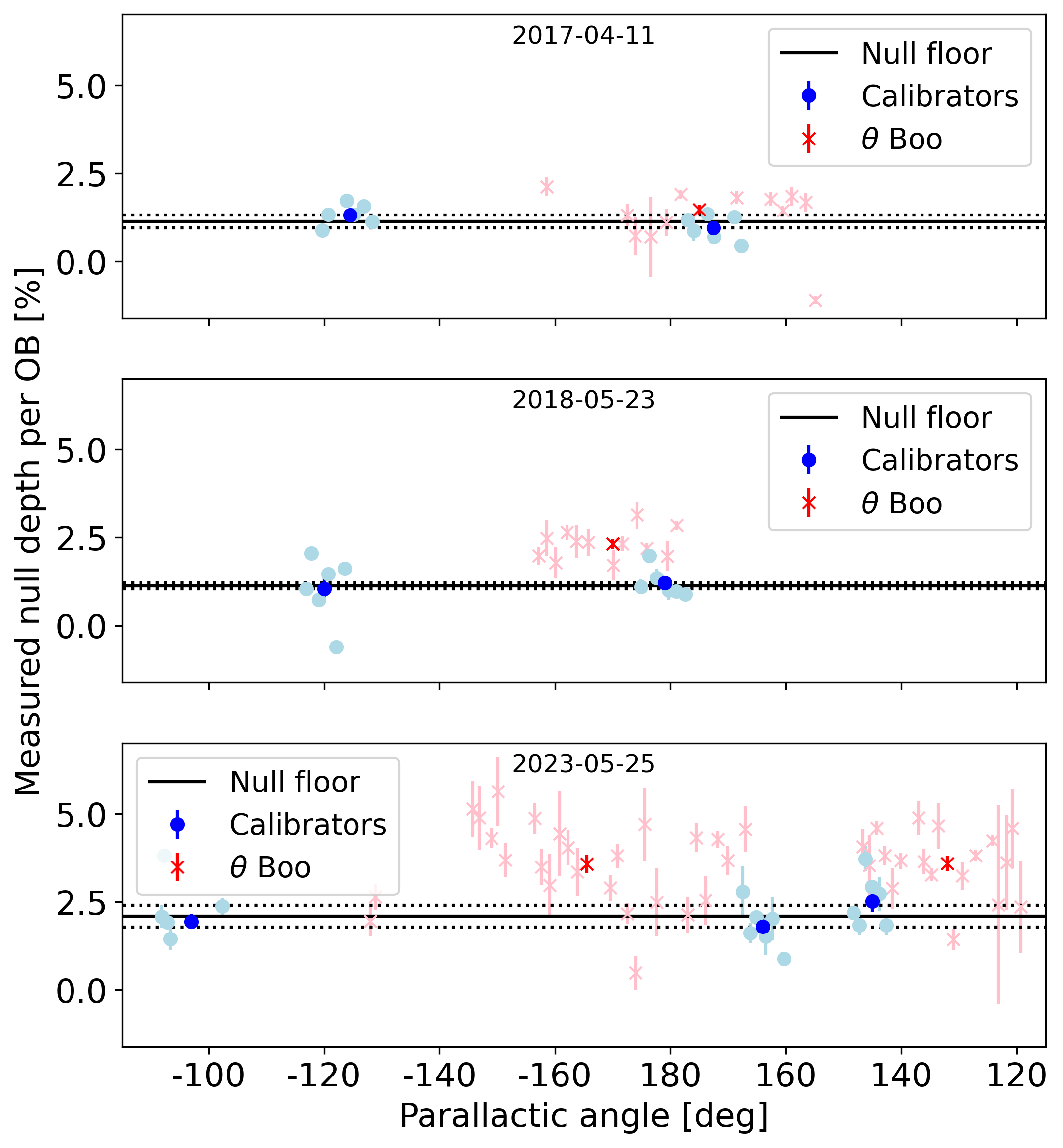
Figure 3: Null depths obtained after the data reduction pipeline described in Sec 3.1. These points are all computed using the reduction pipeline with an aperture radius of 24 pixels (i.e., 430 mas). The OBs are plotted with regards to their parallactic angle (left) and their UT of observation (right). The OBs are plotted for each of the three nights of observation: 2017 April 11 (top), 2018 May 23 (middle), and 2023 May 25 (bottom). For each figure, the light blue points and light red crosses are showing the measured null depth of the OBs for the calibrators and $\theta$ Boo respectively. The dark blue points and dark red crosses are the null depth values for each pointings, corresponding to the unweighted mean values of the OBs included in the pointing. The instrumental null depths measured from the calibrators are averaged to calculate the null floor, which corresponds to the reference level below which any excess would not be reliably detected. The null floor and its error bar are shown with the solid and dotted black lines respectively. The error bar corresponds to the 1$\sigma$ standard deviation.

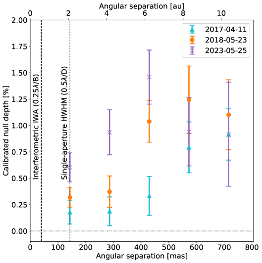
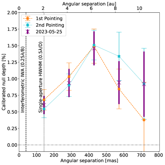
Figure 4: Left: calibrated null depths for the different aperture radii and for the three nights of observation with NOMIC. The aperture radii are: 8, 16, 24, 32, and 40 pixels (i.e., 143, 286, 430, 573, and 716 mas, respectively). Right: calibrated null depths for the 2023 May 25 observation and for the different aperture radii. The results for the two individual pointings are shown (dotted and dashed lines) together with the combined results (crosses). The first pointing corresponds to the OBs taken from 04:00 to 06:00 UT the second pointing is from 06:30 to 07:30 UT.

3.2 L’-band direct imaging data

The LMIRCam data were processed using the LBTI Exozodi Exoplanet Common Hunt (LEECH) survey pipeline (see Stone et al., 2018). The pipeline first replaces any bad pixels by using the median of the eight nearest pixels. Similarly to the N’-band observations, the thermal background is subtracted using the median value of the opposite nod images from the closest OB. The images are then coarsely corrected for distortion using the de-warp coefficients from Maire et al. (2015) which are still sufficiently precise as astrometric precision is not required. The PSF of the telescope has a FWHM of 95 mas at 3.7 µm. The pixels of the detector have an on-sky size of 10.7 mas, so the PSF is over-sampled by around a factor 4. Each image is thus binned 2$\times$2 to remove cosmic rays or any remaining bad pixels.

The pipeline then fitted and removed the diffracted light from the star using PCA Amara & Quanz (2012); Soummer et al. (2012); Gonzalez et al. (2017) before de-rotating the images and stacking them. To optimize the high-contrast capability, the PCA method was performed annulus by annulus with 9 pixels width ($\sim 2\lambda/D$) and an annulus of 1 pixel width as a subtraction region. Fake planets were injected at different angular radii, the number of components for the PCA is chosen to maximize their SNR. The best contrast is reached after several iterations. The planets injection and the contrast estimation procedures are detailed in Wagner et al. (2019). The two nod positions are separately reduced but their images are recombined using a weighted mean. The weights are set for each annulus to optimize the detection of the fake planets. Regions of poor sensitivity from dust diffraction within LMIRCam can be down-weighted.

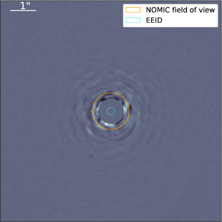
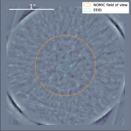
Figure 5: Left: ADI image of $\theta$ Boo from LMIRCam after processing with the LEECH-survey pipeline. The image has a FOV of 4″. The central mask of 5$\lambda/D$ radius is used to improve the visualization. No feature indicating the presence of a companion is detected between 0.3″ and 4″. Right: ADI image of $\theta$ Boo from SHARK-NIR after processing with the SHARP pipeline using 5 components for the PCA. The image has a FOV of 1.3″. For both images, the outer circle indicates the coherent FOV of NOMIC in the N’-band ($\sim 670$ mas from Eq. (1)), and the inner dashed circle represents the EEID ($\sim 138$ mas). No feature indicating the presence of a companion is detected between 0.15″ and 1.3″.

Figure 5 (left) shows the reduced image of $\theta$ Boo. No feature resembling a companion can be observed between 0.3″ and 4″. The detection limits corresponding to this observation are presented in Sec. 4. To account for the reduction of resolution elements close to the star – and its impact on the confidence level of the detection thresholds – the detection limits are calculated including small sample statistics (Mawet et al., 2014).

3.3 NIR direct imaging data

The SHARK-NIR data are reduced using the Python pipeline called SHARP, currently under development. The pipeline first subtracts the dark and divides the image by the flat. The internal deformable mirror generated four satellite spots that are images of the star with lower brightness and symmetric with respect to the position of the target. They were arranged in a cross configuration that can be used to determine the position of the star behind the coronagraph. Fitting two lines through two opposite spots, their intersection accurately defines the central position of the stellar PSF. Bad quality frames are also removed, for example when not adequately masked by the coronagraph because of bad weather conditions. After this procedure, we are left with 6422 frames. To improve the reduction time, the frames are grouped in groups of four and averaged, which forms a datacube of 1605 frames. On this datacube we perform the speckle subtraction based on the PCA algorithm, before de-rotating the images and stacking them. The PCA is used with 1, 5, 10, 15, 20, and 25 components. For each number of components, a reduced image is obtained. However, no significant differences are observed between the different images.

Figure 5 (right) shows the resulting SHARK-NIR image using 5 components for the PCA. No feature resembling a companion can be observed between 0.15″and 1.3″. We then calculate the brightness contrast considering the standard deviation in one pixel wide ring and divide it for the normalization factor obtained using the non-coronagraphic images described in Sec. 2.4. The detection limits corresponding to this observation are presented in Sec. 4. Similarly to the LMIRCam data, the detection limits are calculated while accounting for small sample statistics.

4 Detection limits in the L’-band and NIR

The images obtained from LMIRCam and SHARK-NIR after post-processing (Fig. 5) show no apparent point-like feature. They can still be used to compute companion detection limits of the observations. Figure 6 gives these detection limits (corresponding to SNR=5) as a contrast curve with respect to the angular separation with the star. The constraints in planetary masses are given from the evolutionary model COND described in Baraffe et al. (2003). The model assumes a “hot start” formation scenario where the gravitational instabilities in the protoplanetary disk are causing the dust and gas to collapse and form the planet (Spiegel & Burrows, 2012). The collapsing gas conserves its entropy, which gives the planet a high initial entropy. The COND model ignores dust opacity by assuming that the dust in the atmosphere of the planet immediately falls below the photosphere after formation. Given the contrast curves from the images and the stellar parameters, the model computes the planetary masses corresponding to different contrast levels. The best detection limit is achieved in the NIR by SHARK-NIR with a limit of 11 $M_{\text{Jup}}$ around 1.3″. The LMIRCam is unable to probe the planetary regime of masses with a limit of 18 $M_{\text{Jup}}$ for separations $>$1.5″.

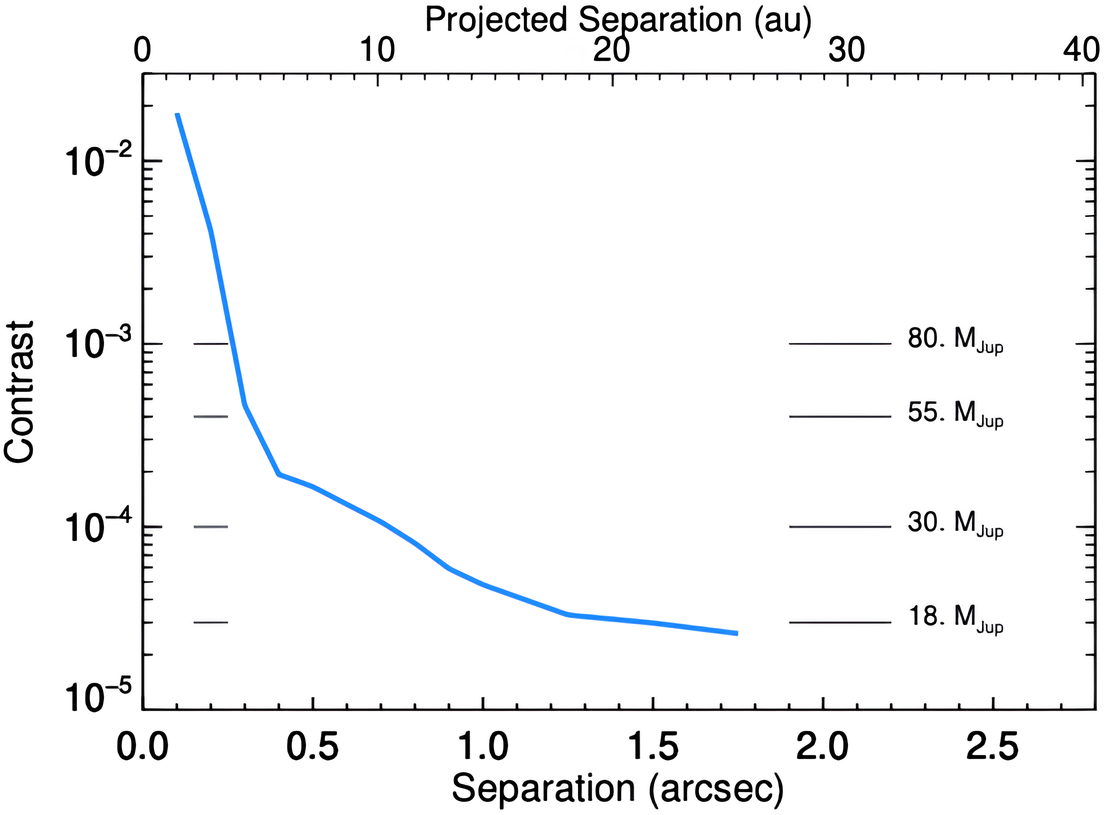
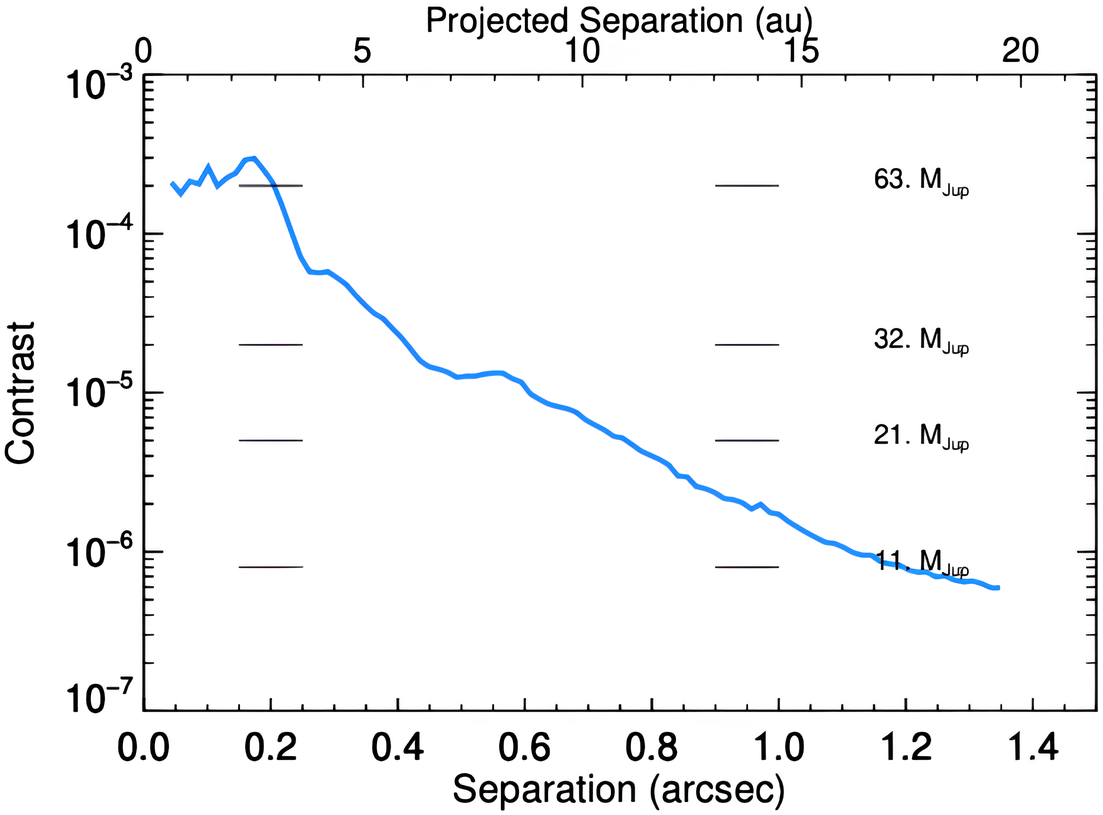
Figure 6: Detection limits for companions around $\theta$ Boo in the L’-band with LMIRCam (left) and in the H-band with SHARK-NIR (right). The blue line shows the contrast with regards to the angular separation. For four levels of contrast, the detection limit is given in terms of mass (in units of Jupiter mass). Observations in the H-band give the best mass constraint around 1″with a limit of 11 $M_{\text{Jup}}$. The system is assumed to be 500 Myr for these mass constraints.

The mass constraints for these observations are calculated assuming an age of 500 Myr for $\theta$ Boo from Gáspár et al. (2013). The age of the system is however uncertain according to the different methods used to calculate it. Table 4 gives a resume of the current estimates for each method. The result goes from 400 Myr to a few Gyrs. Rachford & Foight (2009) reported that $\theta$ Boo is about twice as luminous as a zero-age main-sequence star of the same color. This implies that the star is either at the end of its main-sequence phase or a binary with equal components. Using the Stefan-Boltzmann law with the stellar parameters listed in Table 1 gives a stellar radius of 1.77 R_⊙. Interferometric observations performed at the Center for High Angular Resolution Astronomy (CHARA) measured a stellar radius of $1.73\pm 0.01$ R_⊙ (Boyajian et al., 2013). The theoretical and measured stellar radii are found to be about 30 % larger than a zero-age F7V star (i.e., 1.324 R_⊙, Pecaut & Mamajek, 2013). This means that $\theta$ Boo is likely at the end of its main-sequence phase and not a binary with equal components. Its age is therefore in the higher estimates of Table 4, between 3 and 4.7 Gyr. However, for an age beyond 500 Myr, the internal heat resulting from planet formation has already dissipated and there should not be any significant difference for the evolutionary model. The mass limits are therefore still relevant even for this age range. It should also be mentioned that $\theta$ Boo has a detected binary companion with a separation of 70″($\sim$1000 au) (Eggen, 1956). This separation is however too large to impact the presence of debris disk in the system (Yelverton et al., 2019).

Table 4: Summary of the age estimates of $\theta$ Boo from different independent methods.

Method	Estimated age [Gyr]	References
Isochrones	2.9-4.7	(1)
Chromospheric activity	0.4-0.9	(2)
X-ray emission	0.4	(3)

References. (1) Marsakov & Shevelev (1995); Lachaume et al. (1999); Holmberg et al. (2009); Boyajian et al. (2013); Luck (2017); (2) Barry (1988); Vican (2012); Gáspár et al. (2013); Stanford-Moore et al. (2020); (3) Vican (2012).

5 Dust modeling

In this section, we set constraints on the exozodiacal dust spatial distribution. We first describe the dust emission models used to represent the exozodi emission. These emission models are then combined with an MCMC fitting procedure. This allowed us to recover information at different epochs on the shape of the exozodiacal dust disk around $\theta$ Boo, and thus to explore its temporal evolution.

5.1 Model description

Here we describe how we generate exozodiacal dust emission models to be compared with the LBTI observations shown in Fig. 4. Our models are based on the framework presented in Kennedy et al. (2015) – which was used as baseline for the HOSTS survey at the LBTI.

In this framework, exozodiacal dust disks are assumed to be both optically and vertically thin. The face-on surface density of the dust $\Sigma$ at a distance $r$ to the star is assumed to follow a power-law distribution

$$\Sigma(r)=\Sigma_{0}\times r^{\alpha},$$ (2)

between inner and outer radii $R_{\text{in}}$ and $R_{\text{out}}$, respectively, and with $r$ expressed in au. $\Sigma$ represents the disk’s surface density of cross-sectional area, hence it is expressed in au²/au², and is analogous to optical depth. $\Sigma_{0}$ is the surface density at 1 au, and $\alpha$ is the surface density slope of the disk. The dust surface brightness $S$ at wavelength $\lambda$ is then given by

$$S(r)=2.35\times 10^{-11}\Sigma(r)B_{\nu}(\lambda,T_{\text{d}}(r)),$$ (3)

with $B_{\nu}$ being the dust grain emission at temperature $T_{\text{d}}$. The numerical factor of $2.35\times 10^{-11}$ converts the surface brightness to units of Jy.arcsec^-2. The temperature $T_{\text{d}}$ is that of a blackbody and is defined by

$$T_{\text{d}}=278.3L_{\star}^{0.25}r^{-0.5}\,K,$$ (4)

We summarize the parameters describing the dust spatial distribution in Table 5. The stellar parameters used to compute the dust emission can be found in Table 1.

Geometry of the system

The face-on dust distributions allowed in the model are limited to centrosymmetric geometries with the following parameters: the inner radius $R_{\text{in}}$, the outer radius $R_{\text{out}}$, the dust density at 1 au $\Sigma_{0}$, and the dust density slope $\alpha$. We define the mean radius of the belt with $R=(R_{\text{in}}+R_{\text{out}})/2$. Three different geometries are considered when modeling the observations:

1. A “wide ring” model with free $R_{\text{in}}$ and $R_{\text{out}}$, and fixed $\alpha=0$;

2. A “thin ring” model with free $R_{\text{in}}$, fixed $(R_{\text{out}}-R_{\text{in}})/R=0.1$, and fixed $\alpha=0$. “Thin ring”is a sub-model of the “wide ring” that is useful to constrain the region where most of the dust emission is located;

3. A “disk” model with $R_{\text{in}}$ fixed at the sublimation radius of silicates (corresponding to $T_{\text{BB}}=1500$ K), $R_{\text{out}}$ fixed at an arbitrarily large distance (typically for $T_{\text{BB}}=88$ K), and free $\alpha$. For $\theta$ Boo, $R_{\text{in}}$ and $R_{\text{out}}$ are calculated to be at 0.07 and 20 au respectively (i.e., 4.7 and 1380 mas).

$\Sigma_{0}$ is systematically included as a free parameter for each of the geometries, and constrained in the range [0, $10^{-2}$]. $R_{\text{out}}$ is constrained in the range [0, 20″], and $R_{\text{in}}$ in the range [0, $R_{\text{out}}$[. The range of $\alpha$ is [-10, 10]. For the “wide ring” and “thin ring” models, we choose $\alpha=0$ as a way to simulate a dust belt with a uniform optical depth radial distribution. This assumption is indeed used to study the collisional evolution of cold debris disks, as in Wyatt et al. (2011) (see the P-R drag model description in Sec. 6.2).

Orientation of the system

The orientation of the disk is defined by two parameters: the disk inclination $i$, and the disk position angle “PA”. As mentioned in Sec. 3.1, the 2023 null depths show no visible dependence with the parallactic angles – and hence with the transmission map orientation – which indicates that the disk inclination is expected to be close to face-on ($i=0\degree$) under the assumption of a vertically thin disk. Several preliminary test runs established that the MCMC procedure did not converge in reasonable computational times when fitting the geometry ($R_{\text{in}}$, $R_{\text{out}}$, $\Sigma_{0}$, $\alpha$) and orientation parameters ($i$, PA) simultaneously. We therefore assume the disk to be face-on, and perform the MCMC procedure with $i$ systematically sets to $0\degree$ for the different datasets. The value for PA is then irrelevant.

Table 5: Dust model parameters and their reference values for the zodiacal disk.

Symbol	Unit	Parameter	Reference
$R_{\text{in}}$	au	Inner disk radius	0.034
$R_{\text{out}}$	au	Outer disk radius	10
$R$	au	$(R_{\text{in}}+R_{\text{out}})/2$	5
$\Sigma_{0}$	au2/au2	Surface density at 1 au	$7.12\times 10^{-8}$
$z$	zodi	Surface density at EEID	1
$\alpha$	-	Surface density slope	-0.34
$i$	°	Disk inclination	-
PA	°	Disk position angle	-

Notes. Reference values taken from Kennedy et al. (2015).

5.2 Modeling strategy

Our goal is to model the dust emission as measured with NOMIC. The next step is therefore to compute the dust raw radiance $F_{\text{dust}}$ by integrating Eq. (3) over the passband of NOMIC (N’-band: 9.81-12.41 µm), taking into account the transmission of the NOMIC filter. $F_{\text{dust}}$ is then normalized by the stellar radiance $F_{\star}$, calculated from its blackbody emission. Finally, the model accounts for the impact of the PSF and of the transmission map on the detected flux: the raw radiance map is first multiplied by the LBTI transmission pattern (Sec. 2.2) and then convolved with the modeled PSF of the LBT. The measured excess can then be estimated by integrating the pixels over the different apertures defined in Sec. 3.1, and compared to the results from Fig. 4. This comparison uses an MCMC approach: we generate 30 walkers with flat priors across all parameters, each allowed to perform 500 sample steps (after a burn-in phase of 1000 models). For each model, we calculate its likelihood function with the LBTI observation and its corresponding $\chi^{2}$. The MCMC then explores the parameter space to minimize the $\chi^{2}$ value of the models. The model with the minimum $\chi^{2}$ is finally returned as the best fit model. Figure 7 shows this modeling procedure as applied to the 2023 May 25 observation. The different steps are detailed, from the computation of raw radiance to the retrieval of the excess signature on the detector. The different photometric apertures used to constrain the dust distribution are also shown, with the coherent FOV calculated from Eq. (1).

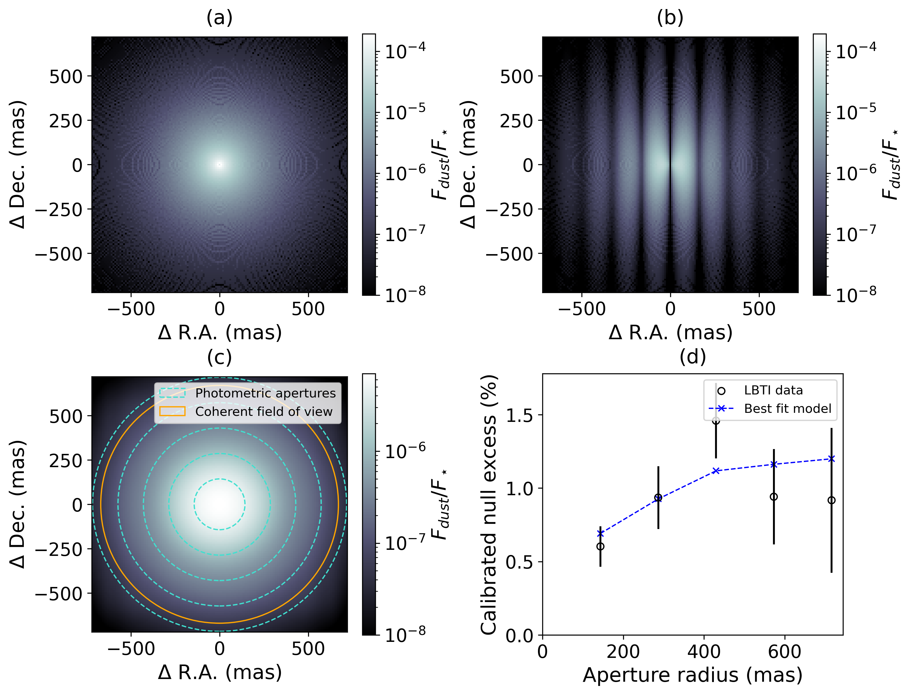
Figure 7: Results of the 2023 May 25 night modeling with the different steps of the procedure. The geometry used is a “disk” with $\Sigma_{0}=3\times 10^{-5}$ and $\alpha=0$, the orientation is face-on. From (a) to (d) are shown: the angular distribution of $F_{\text{dust}}/F_{\star}$, the impact of the LBTI transmission map, the convolution with the PSF of the LBT, and the comparison between the observed excess and the modeled one. For (c), the photometric apertures used in the reduction are indicated with the dashed circles. The coherent FOV is indicated with the solid orange circle. The maps have a pixel size of 10 mas.

Table 6: Results of the modeling for the combined and individual 2017, 2018, and 2023 datasets using the “disk”, “wide ring”, and “thin ring” geometries.

Observing night(s)	Geometry	$\Sigma_{0}/10^{-5}$ [au2/au2]	$R_{\text{in}}$ [au]	$R_{\text{out}}$ [au]	$\alpha$	$z$	$\chi^{2}$	$\chi^{2}_{\text{red}}$
All nights	Disk	$\boldsymbol{0.86^{+0.32}_{-0.28}}$	0.07	20	$\boldsymbol{1.38^{+0.38}_{-0.43}}$	$305^{+34}_{-44}$	$34.4^{+2.78}_{-1.11}$	$2.65^{+0.21}_{-0.09}$
	Wide ring	$\boldsymbol{7.30^{+2.75}_{-2.12}}$	$\boldsymbol{2.05^{+0.42}_{-0.35}}$	NC	0	$1025^{+386}_{-298}$	$36.0^{+2.62}_{-1.22}$	$3.00^{+0.22}_{-0.10}$
	Thin ring	$\boldsymbol{54.5^{+6.54}_{-5.58}}$	$\boldsymbol{2.95^{+0.53}_{-0.36}}$	$3.25^{+0.58}_{-0.40}$	0	0	$38.9^{+3.40}_{-1.12}$	$2.99^{+0.26}_{-0.09}$
2017-04-11	Disk	$\boldsymbol{0.38^{+0.59}_{-0.26}}$	0.07	20	$\boldsymbol{1.73^{+0.92}_{-1.16}}$	$158^{+62}_{-67}$	$4.31^{+3.93}_{-2.16}$	$1.44^{+1.31}_{-0.72}$
	Wide ring	$\boldsymbol{63^{+180}_{-37}}$	$\boldsymbol{6.17^{+2.02}_{-1.57}}$	NC	0	0	$4.97^{+4.35}_{-1.80}$	$2.49^{+2.20}_{-0.90}$
	Thin ring	$\boldsymbol{186^{+175}_{-87}}$	$\boldsymbol{6.69^{+1.22}_{-1.35}}$	$7.36^{+1.34}_{-1.48}$	0	0	$4.77^{+3.22}_{-1.34}$	$1.59^{+1.10}_{-0.45}$
2018-05-23	Disk	$\boldsymbol{0.78^{+0.46}_{-0.32}}$	0.07	20	$\boldsymbol{1.6^{+0.47}_{-0.54}}$	$322^{+53}_{-64}$	$4.08^{+2.70}_{-1.20}$	$1.36^{+0.90}_{-0.40}$
	Wide ring	$\boldsymbol{14^{+8.1}_{-4.8}}$	$\boldsymbol{2.81^{+0.74}_{-0.62}}$	NC	0	0	$4.81^{+2.69}_{-1.29}$	$2.40^{+1.35}_{-0.65}$
	Thin ring	$\boldsymbol{68.3^{+51}_{-12}}$	$\boldsymbol{3.63^{+0.85}_{-0.69}}$	$4.00^{+0.94}_{-0.76}$	0	0	$6.34^{+3.39}_{-1.34}$	$2.11^{+1.13}_{-0.45}$
2023-05-25	Disk	$\boldsymbol{2.98^{+0.60}_{-0.83}}$	0.07	20	$\boldsymbol{0.05^{+0.69}_{-0.86}}$	$443^{+98}_{-170}$	$4.49^{+2.16}_{-1.23}$	$1.50^{+0.72}_{-0.41}$
	Wide ring	$\boldsymbol{5.52^{+3.67}_{-1.97}}$	$\boldsymbol{1.29^{+0.49}_{-0.75}}$	NC	0	$775^{+515}_{-277}$	$3.76^{+2.37}_{-0.89}$	$1.88^{+1.20}_{-0.45}$
	Thin ring	$\boldsymbol{77.9^{+18.7}_{-29.2}}$	$\boldsymbol{2.42^{+0.54}_{-0.46}}$	$2.66^{+0.60}_{-0.51}$	0	0	$3.44^{+3.48}_{-1.17}$	$1.15^{+1.16}_{-0.39}$

Notes. NC stands for Not Constrained. The parameters fitted by the MCMC are written in bold text with the median values and standard deviations taken from their posteriors, given in Appendix B. The other parameters are either fixed or derived from the fitted ones. The zodi level $z$ is estimated by calculating the ratio between $\Sigma$(r=EEID) and the zodiacal dust density at 1 au (i.e., $7.12\times 10^{-8}$). Values of $z$=0 indicate that $R_{\text{in}}$¿2 au, so no dust is expected at the EEID from the corresponding model.

5.3 Results

First, assuming that the system is in a steady state, the three geometries considered to model the dust spatial distribution – “thin ring”, “wide ring”, and “disk”– are used to fit the combined 2017, 2018, and 2023 datasets. Figure 8 shows the best fit models, and Table 6 summarizes the median values of the model parameters with their standard deviation obtained from their MCMC posterior distributions. All the MCMC posteriors are presented in Appendix B. The median values of the $\chi^{2}$ and reduced $\chi^{2}$ ($\chi^{2}_{\text{red}}=\chi^{2}/\nu$, where $\nu$ is the degree of freedom) are also indicated.

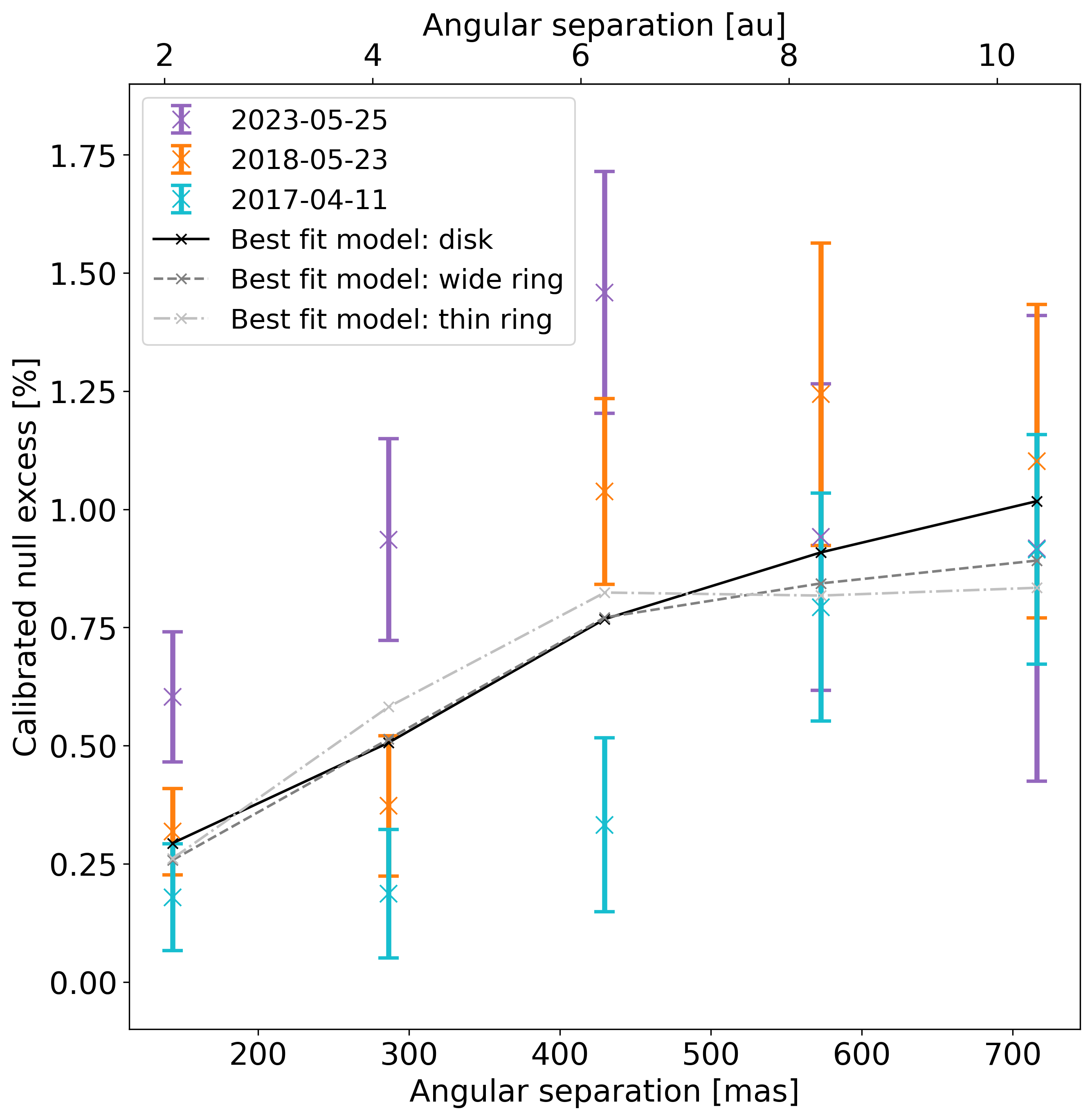
Figure 8: Best fit models for the combined 2017, 2018, and 2023 datasets. The solid dark lines represent the best fit models using a disk geometry, as defined in Sec. 5.1. The dashed gray lines represent the best fit models using a wide ring geometry. The dash-dotted silver lines represent the best fit models using a thin ring geometry. The parameters of the models are listed in Table 6.

The different geometries are then used to fit the individual 2017, 2018, and 2023 datasets. Figure 9 shows the best fit models. The best fit values of $\chi^{2}_{\text{red}}$ are significantly worse when fitting the combined nights compared to the individual nights. The steady state hypothesis for the system is therefore not favored, but cannot be fully rejected. We can note that despite that the “thin ring” is a sub-model explored by the “wide ring” model, their results are not systematically compatible. Indeed, adding $R_{\text{out}}$ as an additional free parameter enables to explore more geometries and find models with better $\chi^{2}$ – although not significantly better. For the individual fits, the different $\chi^{2}$ obtained for each geometry are consistent for the three observing nights. Our data are therefore not able to discriminate between the three possible dust distributions under the assumption of a face-on, optically thin exozodi.

Figure 10 gives the 2D maps of dust radiance for the individual models of 2017, 2018, and 2023, using the median values of the model parameters from Table 6.

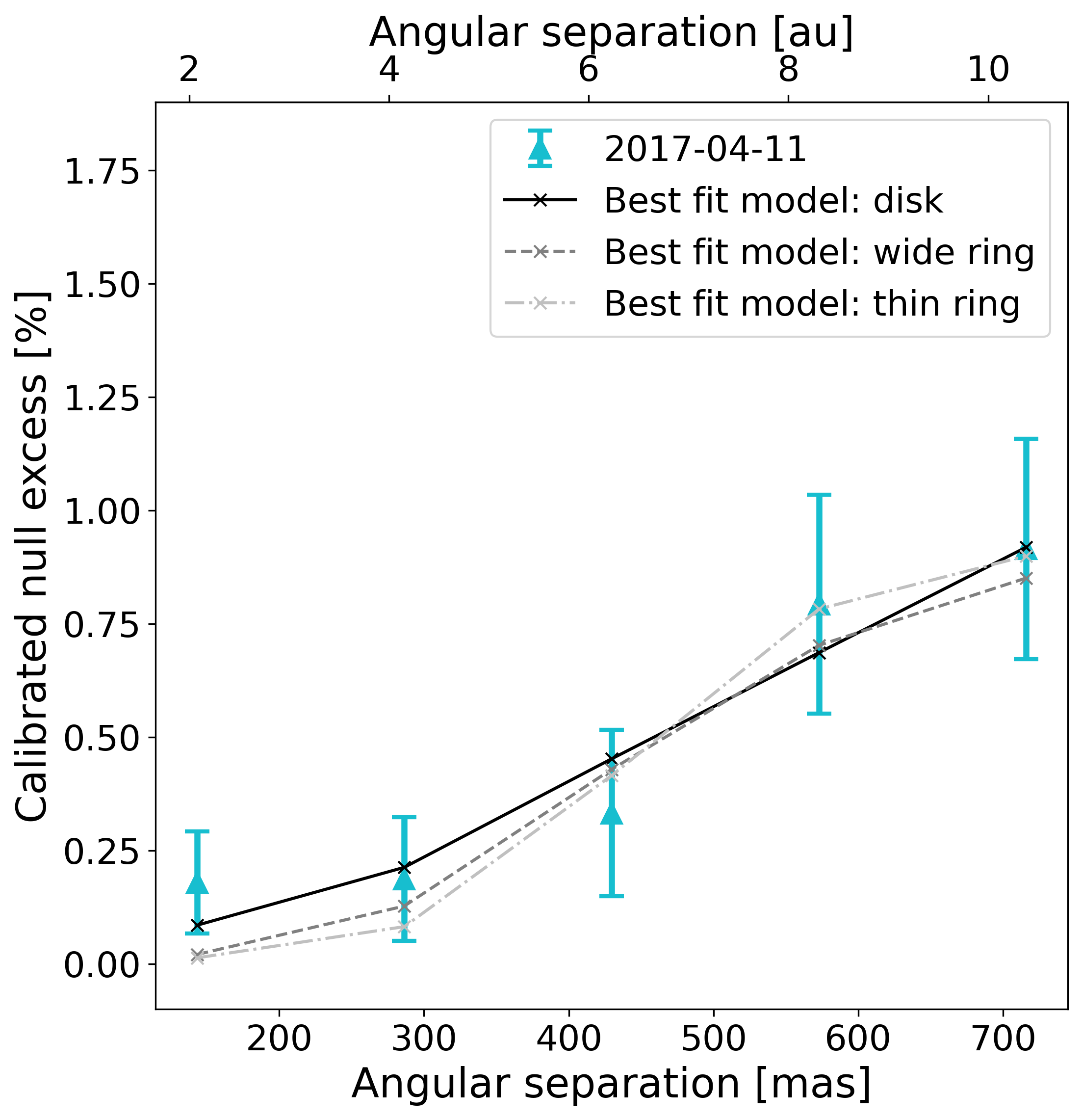
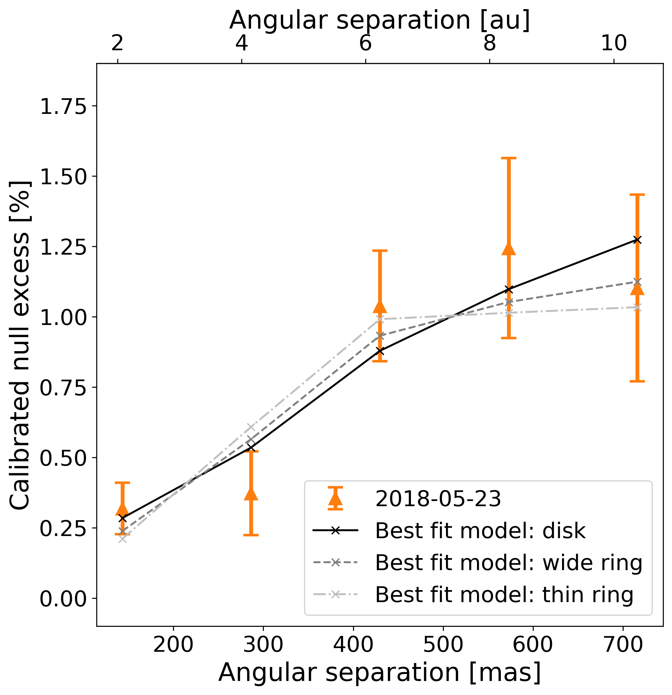
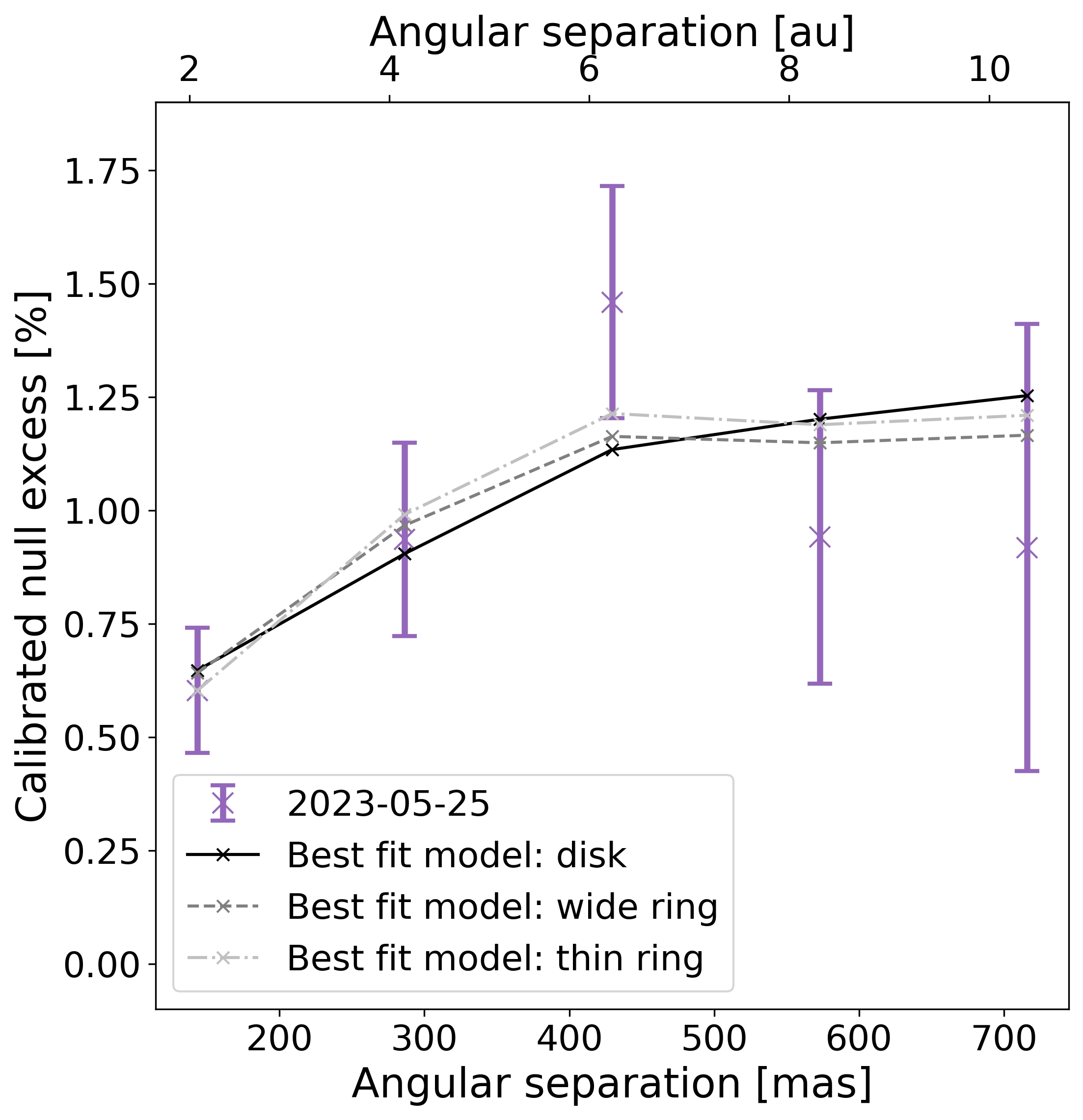
Figure 9: Best fit models for the 2017 (left), 2018 (middle), and 2023 (right) datasets. The solid dark lines represent the best fit models using a disk geometry, as defined in Sec. 5.1. The dashed gray lines represent the best fit models using a wide ring geometry. The dash-dotted silver lines represent the best fit models using a thin ring geometry. The parameters of the models are listed in Table 6.

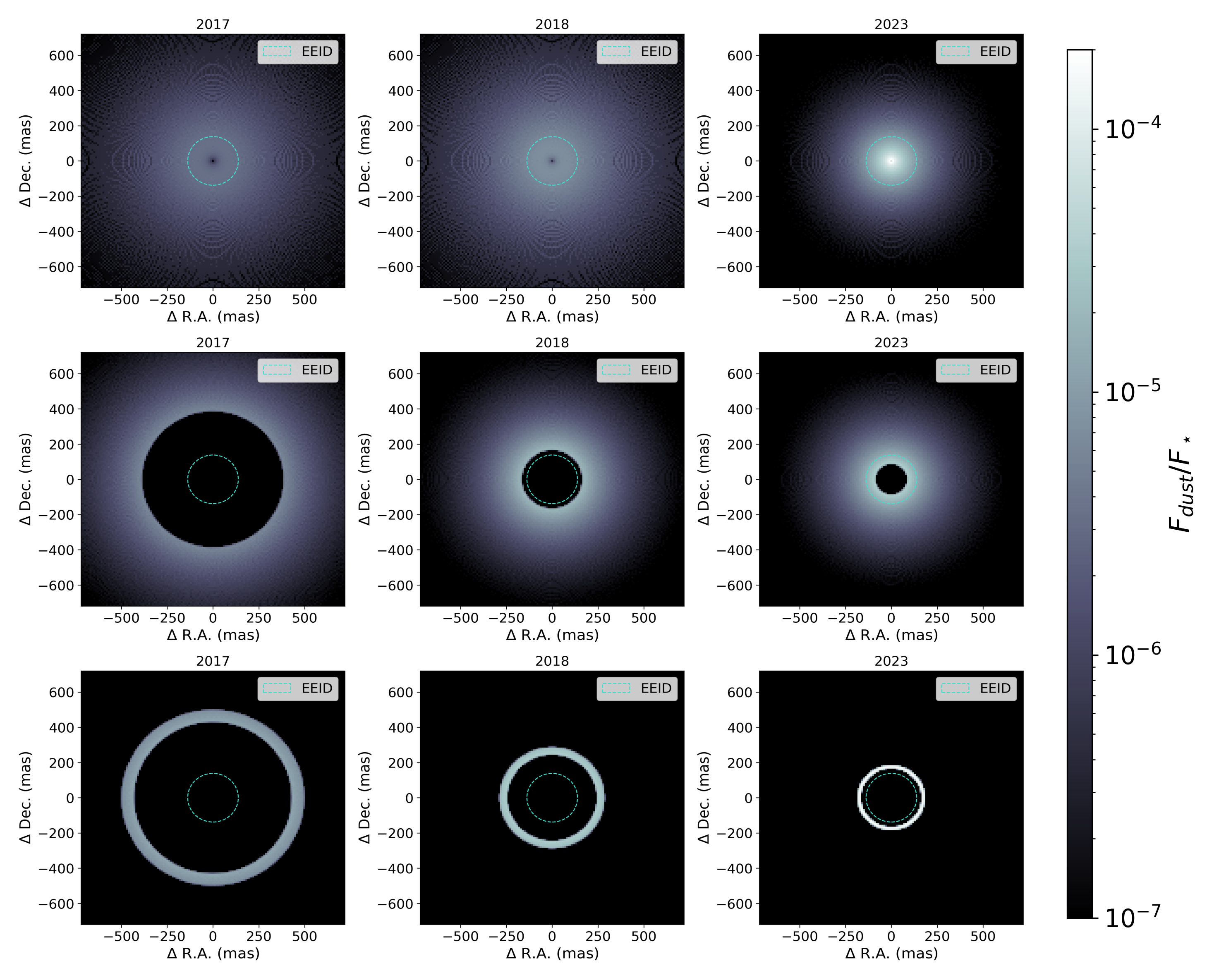
Figure 10: 2D maps of the dust surface brightness ($F_{\text{dust}}$) for the models of 2017 (left), 2018 (middle), and 2023 (right). The maps correspond to the models using the “disk” (top), “wide ring” (middle), and “thin ring” (bottom) geometries. $F_{\text{dust}}$ is normalized by the stellar radiance ($F_{\star}$). Both $F_{\text{dust}}$ and $F_{\star}$ are integrated over the passband of NOMIC. The dashed circle represents the EEID ($\sim$138 mas). The maps have a pixel size of 10 mas.

5.4 Analysis of the dust models

Dust temperature

Equation (3) shows a degeneracy between the dust temperature and the dust density $\Sigma(r)$. For the dust brightness detected by NOMIC, this degeneracy implies that the dust density cannot be precisely estimated without constraining the dust temperature – and hence the dust composition and the size distribution of the grains. The values of $\Sigma_{0}$ in Table 6 are therefore dependent on the assumption that the dust grains behave like ideal blackbodies, and should be considered with caution. Since the nulling observations done at the LBTI are photometric, they cannot constrain the dust temperature using spectral information on the dust emission. Nonetheless, using the same temperatures $T_{\text{d}}(r)$ between the 2017, 2018, and 2023 datasets still allows to compare their $\Sigma$ and estimate the dust variability. Estimates of the dust size distribution, and hence its equilibrium temperature profile, are discussed in Sec. 6.

Dust variability at the EEID

As a probe for the amount of exozodiacal dust expected by the models in the HZ of $\theta$ Boo, we consider the zodi level, $z$. This zodi level is defined as the dust surface density $\Sigma$ at the EEID ($\sim$2 au or 138 mas for $\theta$ Boo) divided by the dust surface density at 1 au in the Solar System (Weinberger et al., 2015). Given that for a disk model, $\Sigma$ is self-consistently calculable for each combination of parameters $\Sigma_{0}$ and $\alpha$ using Eq. (2), we use the MCMC chain samples to build posterior distributions of $z$ for the 2017, 2018, and 2023 “disk” models – $z_{\text{2017}}$, $z_{\text{2018}}$, and $z_{\text{2023}}$, respectively. The resulting median values for the 2017, 2018, and 2023 datasets are shown together with their $1\sigma$ confidence intervals in Table 6. It should be noted that the zodi level obtained for the 2017 dataset is consistent with the one calculated by the HOSTS survey (148.2$\pm$27.7 zodis).

To further quantify the increase in HZ dust brightness found in our models between 2017 and 2023, we calculate the posterior distribution of the ratio $r_{z}=(z_{\text{2023}}-z_{\text{2017}})/z_{\text{2017}}$. From the two MCMC runs of 2017 and 2023, we sample 800 models from each run. We then randomly pair MCMC models from the two epochs for 640,000 times to construct the posterior histogram of the ratio. The posterior can then be integrated to place posterior probabilities on the zodi level increase between epochs. For example, the integral over $r_{z}>2$ denotes the probability that the zodi level has at least doubled between 2023 and 2017. To perform such integration quickly and analytically, we approximate the posterior using a Gaussian kernel density estimate (KDE: Rosenblatt, 1956; Parzen, 1962), which is shown together with the posterior histogram in Fig. 11. The resulting posterior probabilities that there is an increase in zodi level is $93.7\,\%$ (~$1.86\sigma$).

The posterior probability thus suggests a tentative increase of the HZ dust brightness between 2017 and 2023. We note that the probability calculations still make implicit assumptions about the correctness and quality of both the data acquisition (including data calibration and error model) and the dust modeling, and depend slightly on the details of the adopted kernel density estimate. They should thus be handled with caution. The zodi levels calculated for 2017, 2018, and 2023 are also useful to have an order of magnitude of the absolute dust brightness in the HZ of $\theta$ Boo. However, these values are dependent on the chosen dust temperature, which is not well-constrained. Estimates of the zodi level for realistic dust grains with different sizes are given in Sec. 6.

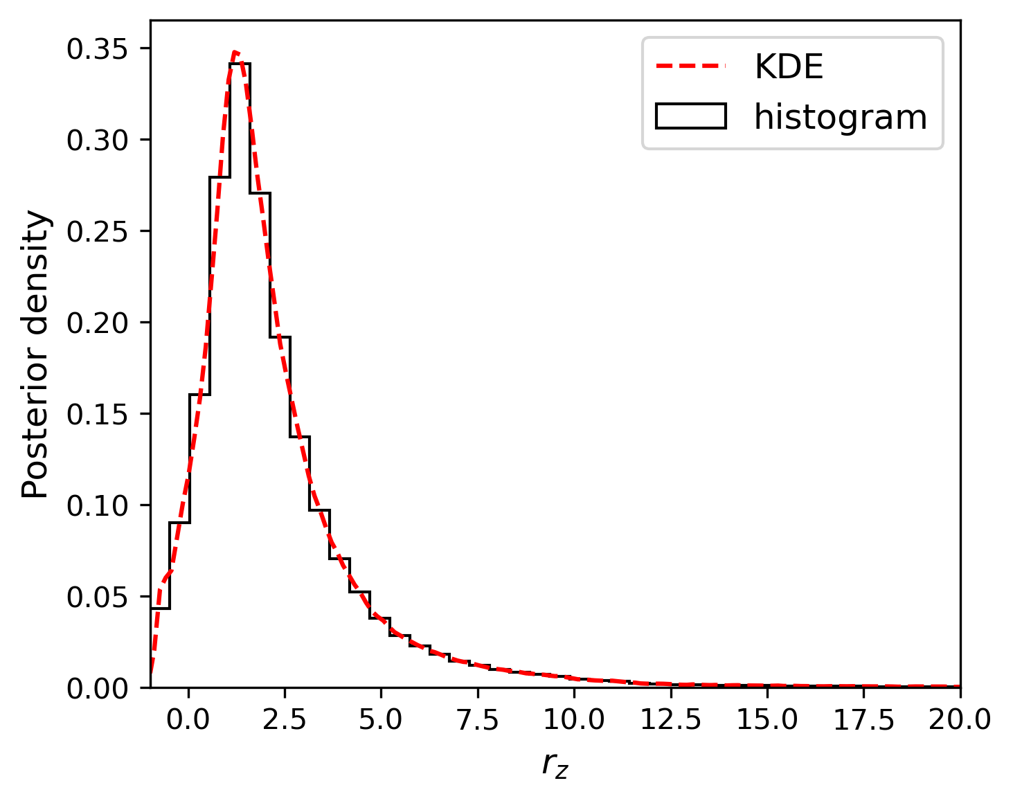
Figure 11: MCMC posterior distribution sample histogram of $r_{z}$, corresponding to the relative difference in zodi level between the 2017 and 2023 models. A Gaussian kernel density estimate (KDE) is used to fit the sample, and to calculate the posterior probabilities of the dust variability.

6 Discussion

6.1 Constraints from the models

SED of the dust models

The LBTI observations around 11 µm are not able to discriminate between the different dust distribution models obtained in Sec. 5 or the properties of the dust grains. One way to constrain their properties further is to simulate the SED from each model, and compare it with the upper limits from Fig. 1. Since the emitting dust may be considerably smaller than the wavelengths, we have to take into account the reduced emissivity $Q_{\text{abs}}$ of realistic grains compared to ideal blackbodies. We assume compact spherical grains composed of amorphous silicates and refractory organics with volume fractions of 1/3 and 2/3, respectively (Li & Greenberg, 1998). We then compute $Q_{\text{abs}}$ and the grains’ resulting equilibrium temperatures with the Mie-type optical properties code of Sommer et al. (2025), which uses the optical constants for the constituent materials from Li & Greenberg (1997). Figure 12 shows the resulting $Q_{\text{abs}}$. We consider grains with diameters of 3, 5, and 10 µm. This choice is motivated by the assumption that the geometrical optical depth is dominated by the smallest grains bound to the system, with an estimated blowout size of around 2.5 µm (calculated with the same grain model).

We retrieve the radial profile of the dust surface brightness $S$ from the models in Fig. 10. For the three grain sizes considered, the optical depth radial profile of the dust $\Sigma$ is recomputed to match its surface brightness with $S$, using the relation

$$\Sigma(r)=\frac{S(r)}{Q_{\text{abs}}(\lambda)\times B_{\nu}(\lambda,T_{\text{d}}(r))}.$$ (5)

Since the surface brightness $S$ is constant between the models with ideal blackbodies (Sec. 5) and the models with realistic grains, they should therefore all fit the data in a similar way. Finally, we choose to cut the optical depth profile of the dust at 10 au (i.e., $\sim$700 mas) for the SED calculation since the dust located outside this distance is out of our coherent FOV. This putative outer dust also has an infrared emission that doesn’t comply with the upper limits, especially for models with a slope $\alpha>1$. We argue that if such quantities of outer dust were present in a static way at these distances, it would have been detected by previous far-infrared observations.

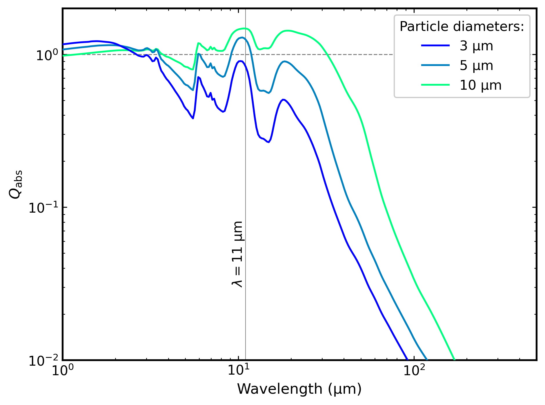
Figure 12: Simulated emissivities for dust grains of size 3, 5, and 10 µm. The volume fraction of the grains is 1/3 amorphous silicates and 2/3 refractory organics.

Figure 13 shows the SEDs corresponding to the recomputed optical depth profiles. Only the SEDs for the “disk” and “wide ring” models are presented for comparison. The SEDs for the “thin ring” models show similar results. We also show the estimate of the mean infrared excess at 11 µm from the present LBTI/NOMIC observations, calculated in Sec. 3.1. This data point serves as a sanity check to verify that all the models are indeed consistent with our observations at 11 µm. It can be noted that no increase is observed at 11 µm between the 2017 and 2023 models. This is because the tentative increase in dust brightness is localized in the inner region of the system, but the dust emission integrated over the entire FOV remains constant for the three observations. This can be seen in Fig. 4 where the data points corresponding to the largest apertures are all consistent.

SED results show that for a grain size of 3 µm, all the models are compatible with the upper limits. For a grain size of 5 µm, a discrepancy with the upper limits around 20 µm wavelength can be noted for some of the models. For a grain size of 10 µm, all models show a significant infrared excess between 20 µm and 50 µm. The simulated SEDs are thus not able to clearly discriminate between the different dust distribution models that we obtained, but they favor a size distribution for the dust between 3 µm and 5 µm to respect the different upper limits. Table 7 gives the new estimates of zodi level from the recomputed optical depth profiles. The zodi levels are found to change by a factor 2.8 for dust grains between 3 and 10 µm.

To constrain further the SED of the dust, we could use observations from the James Webb Space Telescope (JWST: Rigby et al., 2023; Gardner et al., 2023), and more specifically with the Medium Resolution Spectrometer (MRS: Wells et al., 2015; Argyriou et al., 2023) of the Mid-InfraRed Instrument (MIRI: Wright et al., 2023). The measured far-infrared emission could then be compared with our modeled SEDs to identify the dust distribution, but also the dust properties (size, temperature, composition).

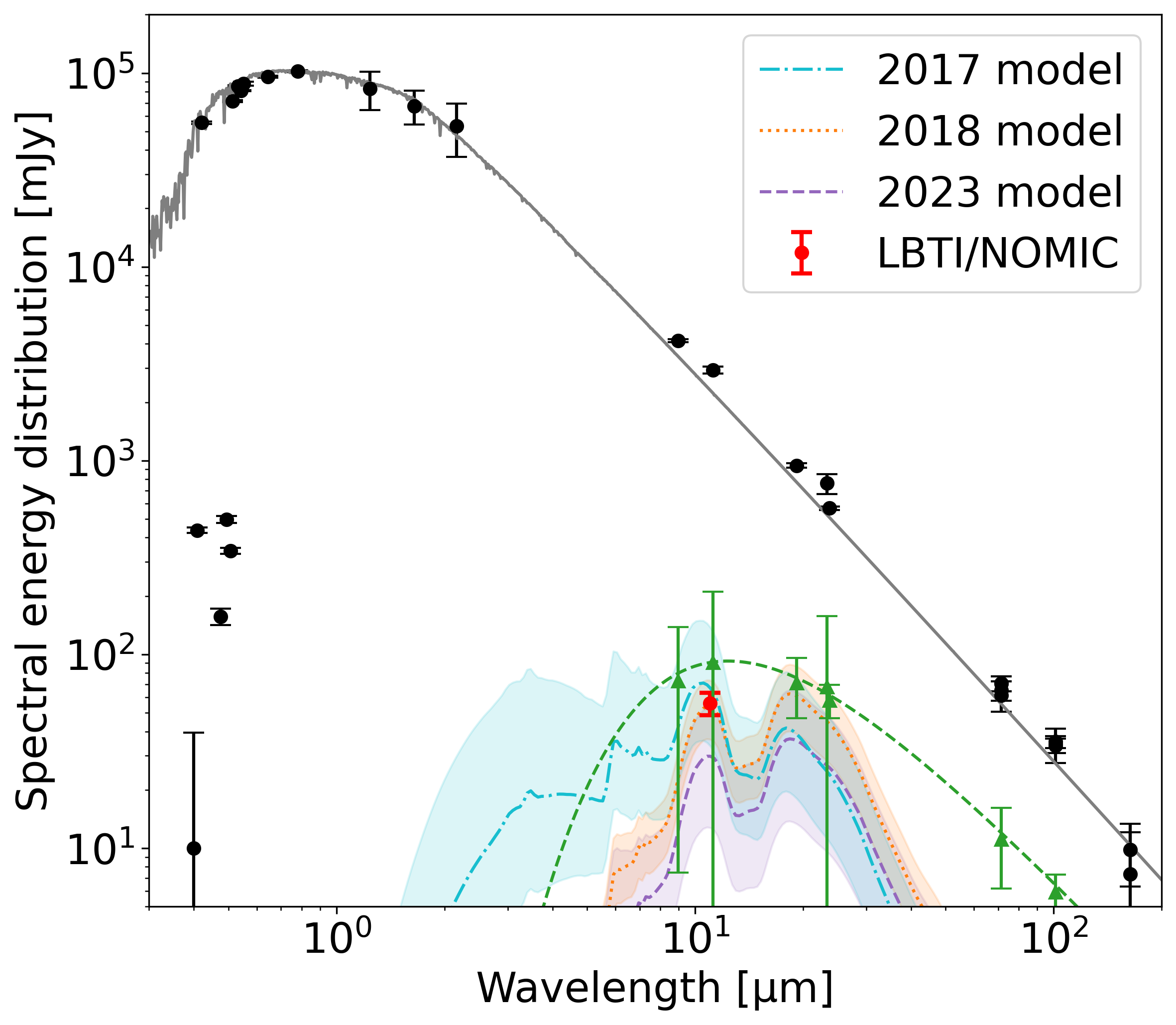
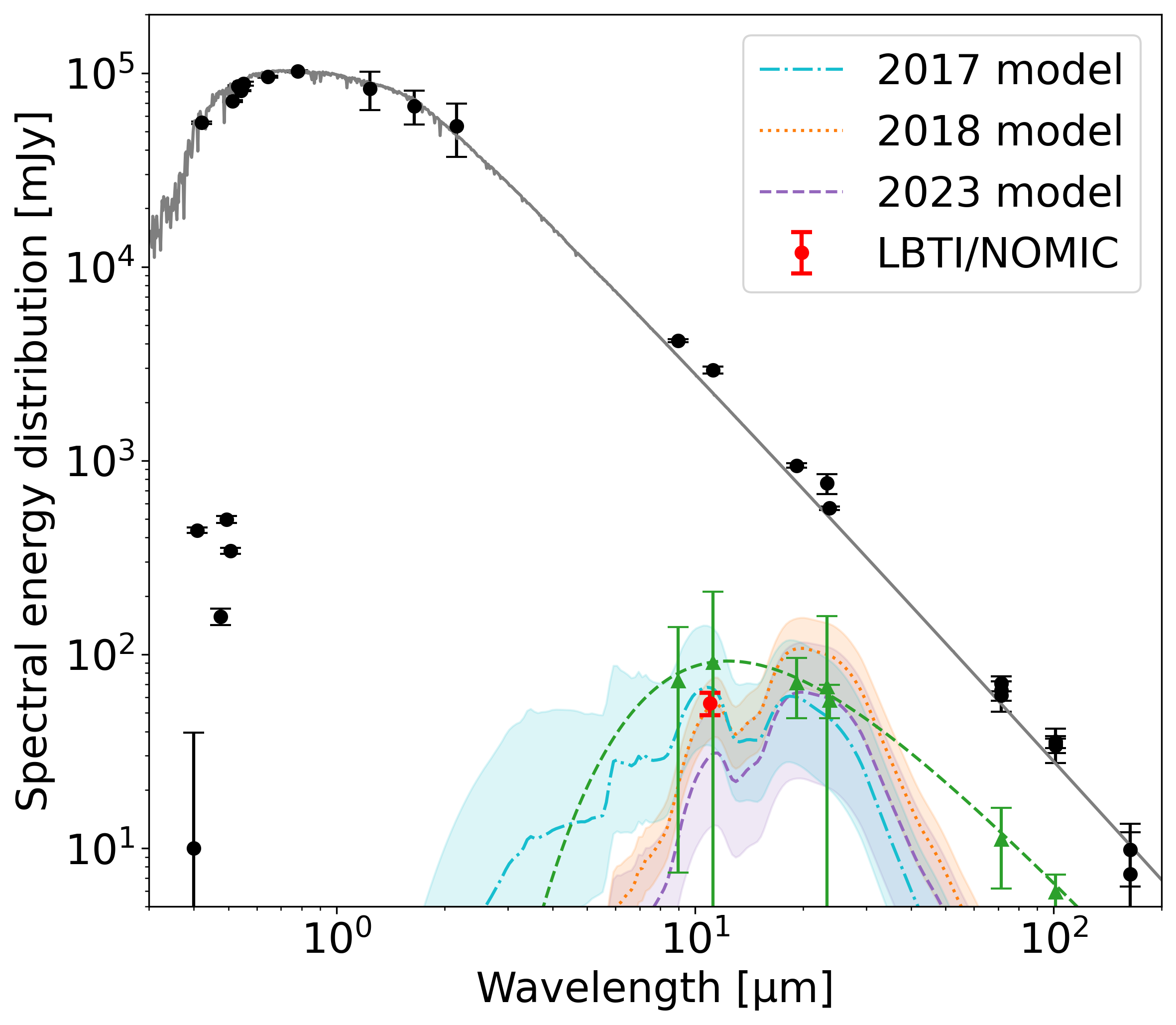
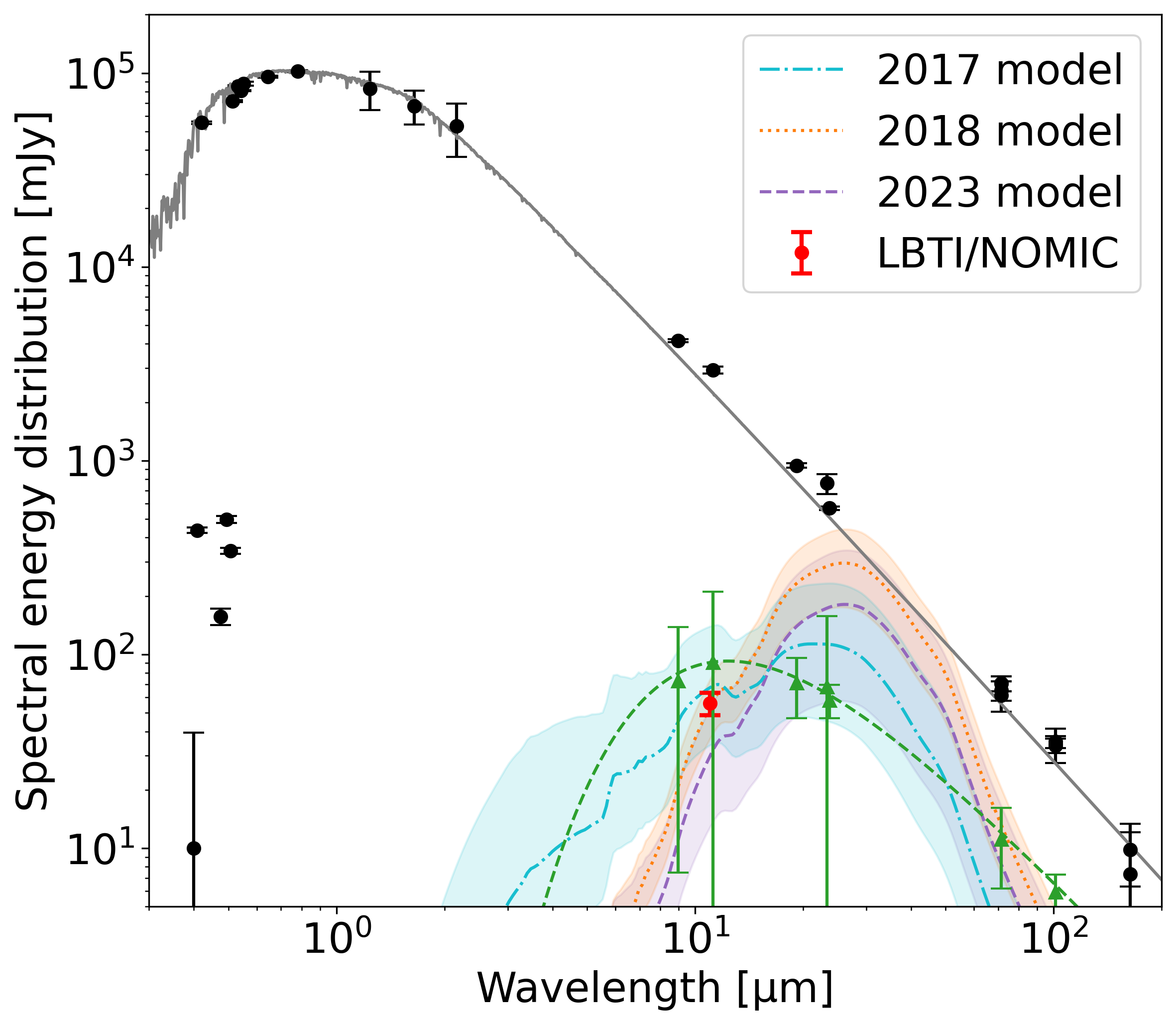
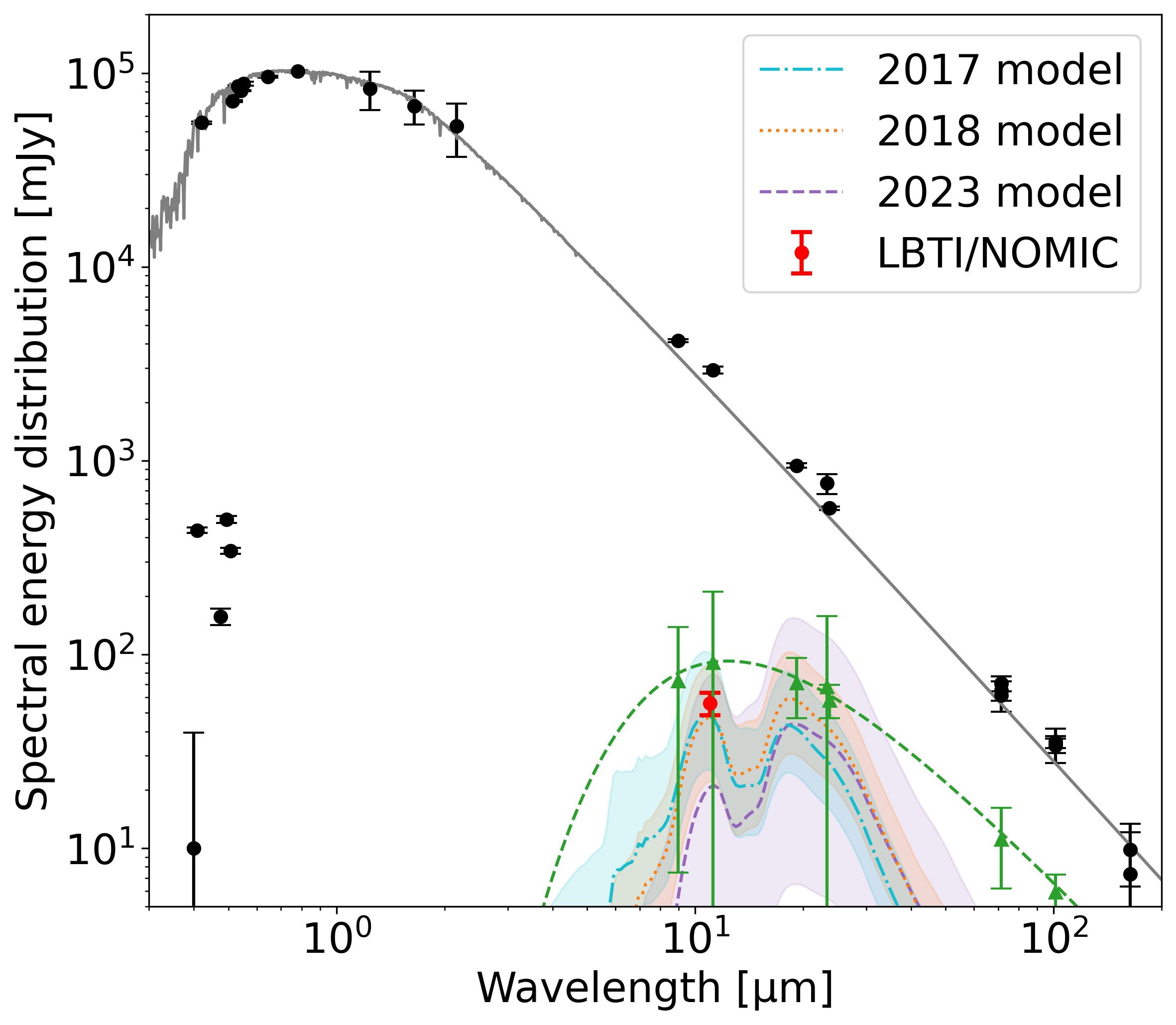
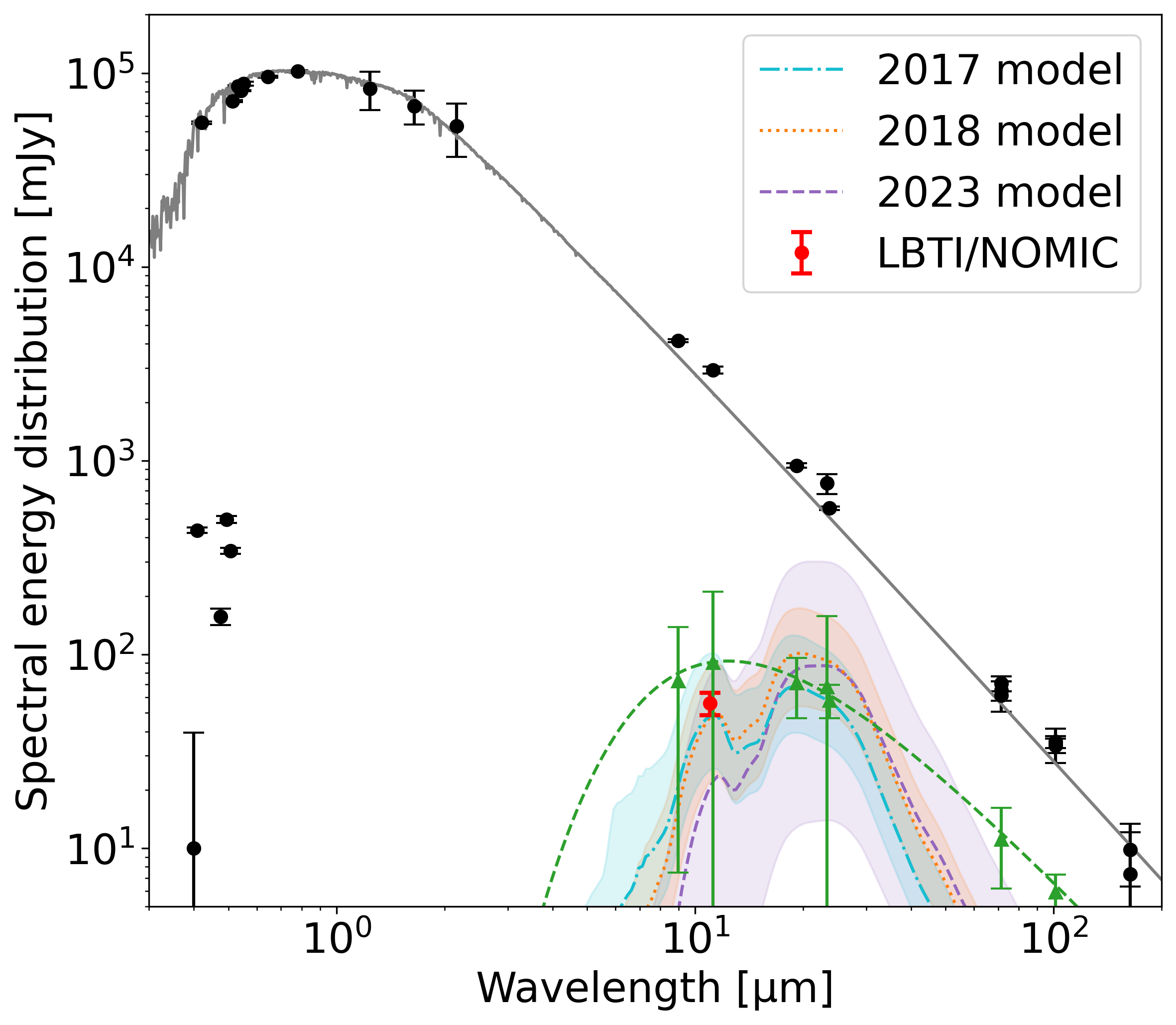
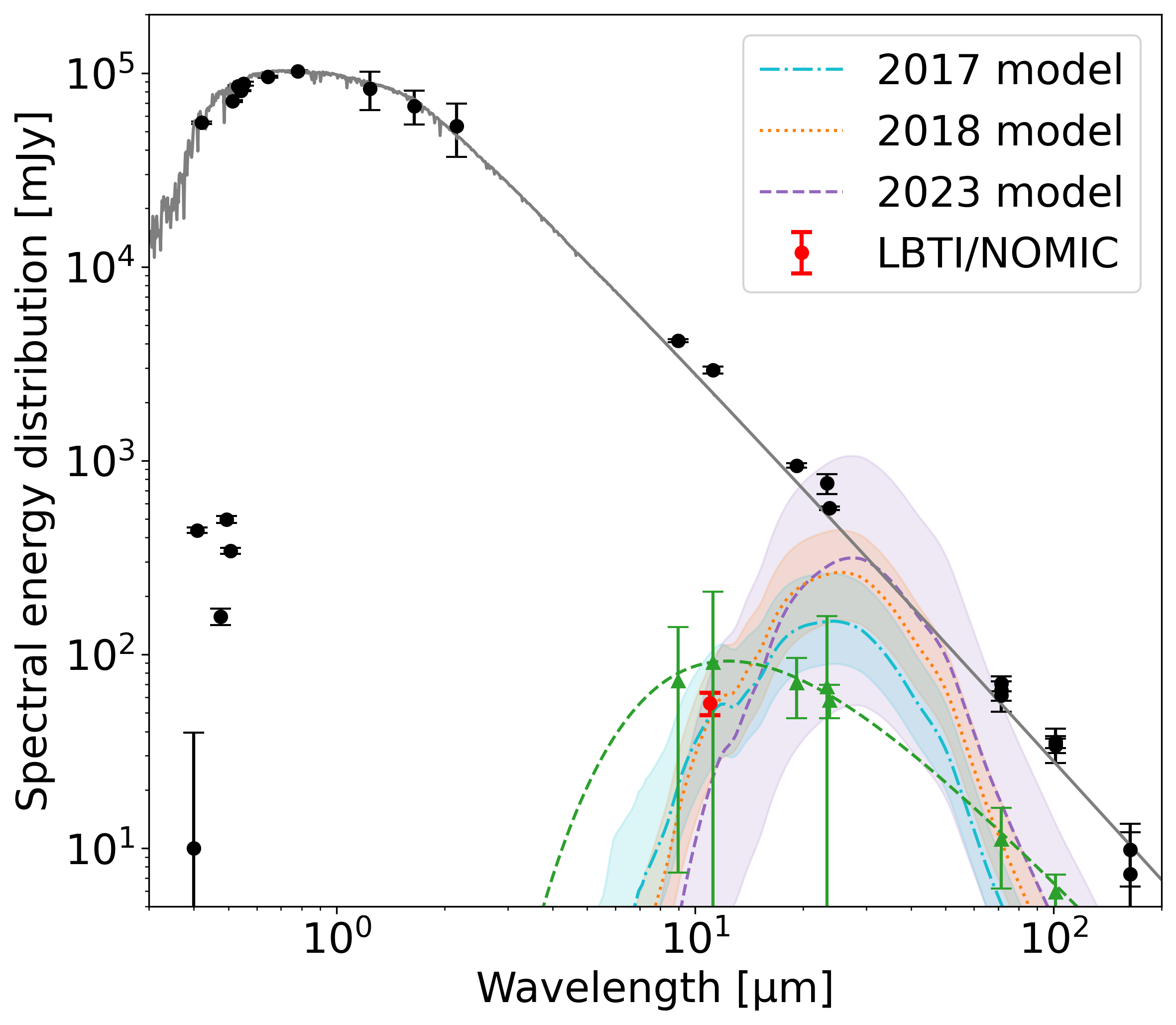
Figure 13: Simulated dust SEDs for realistic dust grains with sizes of 3 µm (left), 5 µm (center), and 10 µm (right). The SEDs correspond to the “disk” (top) and “wide ring” (bottom) models for 2017, 2018, and 2023.

Orientation of the system

The results found in Sec. 3.1 support the hypothesis that the planetary system of $\theta$ Boo has a low inclination – possibly a face-on orientation. This hypothesis is central for the modeling strategy in Sec. 5 but no other independent observations of the planetary system are available to constrain this orientation. It is however possible to constrain the stellar inclination from spectroscopic measurements of $\theta$ Boo. The inclination of debris disks is indeed found to often match with the stellar inclination (Watson et al., 2011; Guilloteau et al., 2011). To determine the stellar inclination, we reproduce the method used in Faramaz et al. (2014) for $\zeta^{2}$ Reticuli. The method uses the color index ($B-V$), the radius $R_{\star}$, and the activity indicator $R^{\prime}_{\text{HK}}$ to estimate the rotational period at the equator of the star using the activity/rotation diagram from Fig. 6b in Noyes et al. (1984). It is then compared with measurements of $\nu\sin(i)$, from which a value of $i$ can be deduced. The stellar properties of $\theta$ Boo are summarized in Table 1, and estimate the rotational period to $P=3.22\pm 0.83$ days and the equatorial rotational velocity to $\nu=27.2\pm 7.1$ km/s. This is consistent with observations giving $\nu\sin(i)=31.8\pm 2$ km/s, which means that the star is likely to be seen edge-on (i.e., with $i\sim 90\degree$). If the exozodiacal disk indeed shares the same inclination as its star, this is incompatible with our LBTI observations for a vertically thin disk. To be compatible, the disk would need to be puffy enough so that no significant changes in null depths would have been observed across the different parallactic angles in Fig. 3. This hypothesis can however not be studied as no models are currently available for the LBTI to simulate observations of vertically thick disks.

The disk may also be misaligned with the stellar rotation axis as a polar circumstellar disk. This configuration has proven to be stable during the stellar lifetime, and can arise from interactions in a young stellar cluster (Kennedy et al., 2012). The wide companion of $\theta$ Boo could have potentially caused such misalignment. The disk may also be tilted or diffused by giant planets orbiting with a planet-disk misalignment (Pearce & Wyatt, 2014; Brady et al., 2023). More observations are therefore required to gather information and constrain the orientation of the planetary system around $\theta$ Boo.

Detection of giant planets

Assuming that the orbit of potential giant planets in the system would share an inclination close to face-on together with the exozodi, this would affect the constraints from radial velocity and transit observations which become thus less severe. Another option would be to study the proper-motion anomaly measured by Gaia EDR3 and model what kind of planets could generate such anomaly (Kervella et al., 2022). Observations of $\theta$ Boo with Gaia are showing a renormalised unit weight error (RUWE) of 3.38, which is enough to indicate the possible presence of a massive body in the system, but might also be explained by the wide companion of $\theta$ Boo.

Table 7: Zodi levels from the recomputed optical depth profiles of the “disk” models for realistic grain sizes of 3, 5, and 10 µm.

	Observing night
Grain size [µm]	2017-04-11	2018-05-23	2023-05-25
3	$63^{+24}_{-26}$	$128^{+21}_{-25}$	$173^{+39}_{-67}$
5	$85^{+33}_{-36}$	$173^{+28}_{-34}$	$235^{+53}_{-91}$
10	$154^{+60}_{-65}$	$313^{+52}_{-61}$	$425^{+97}_{-165}$

6.2 Origin of the dust and its variability

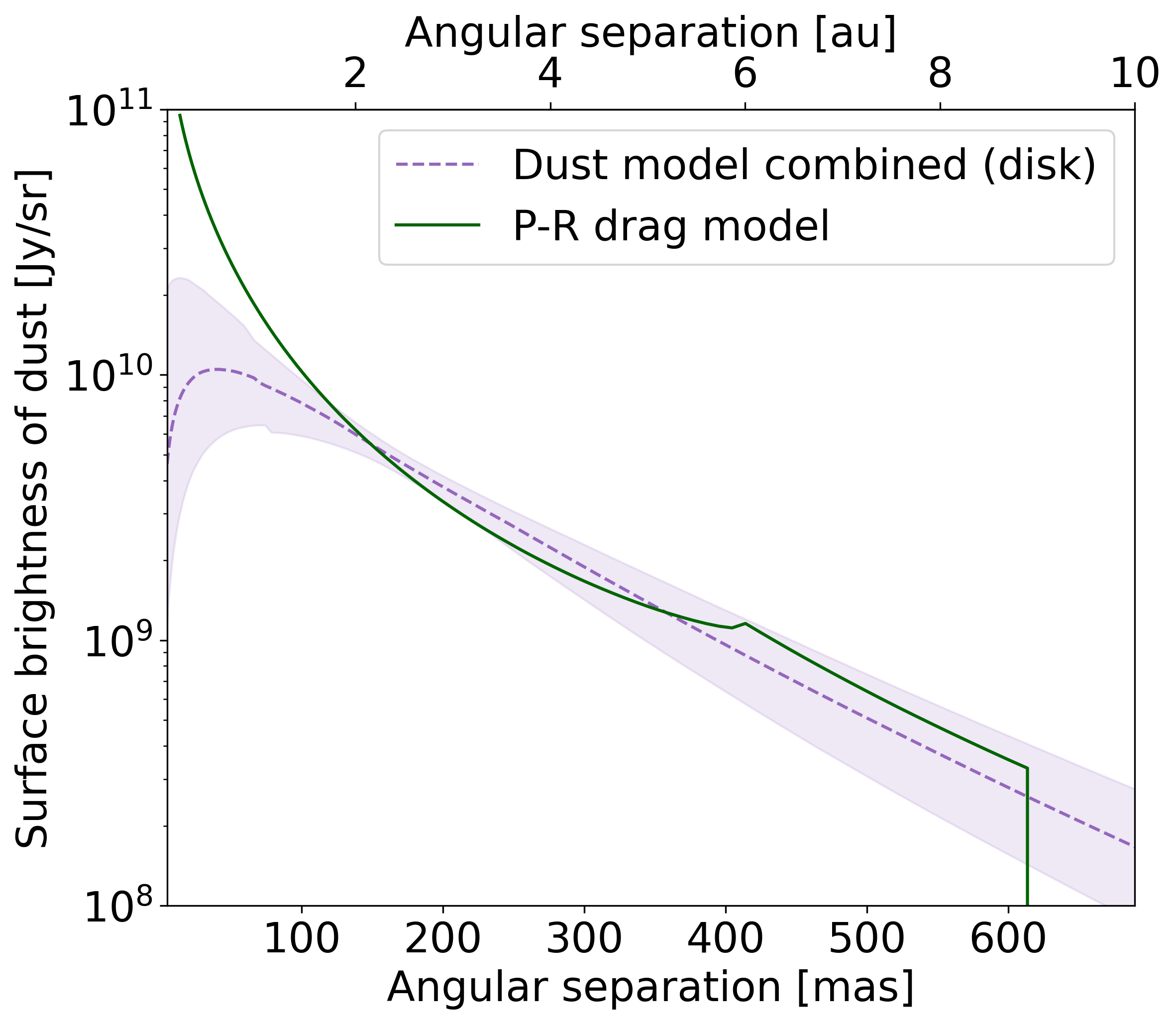
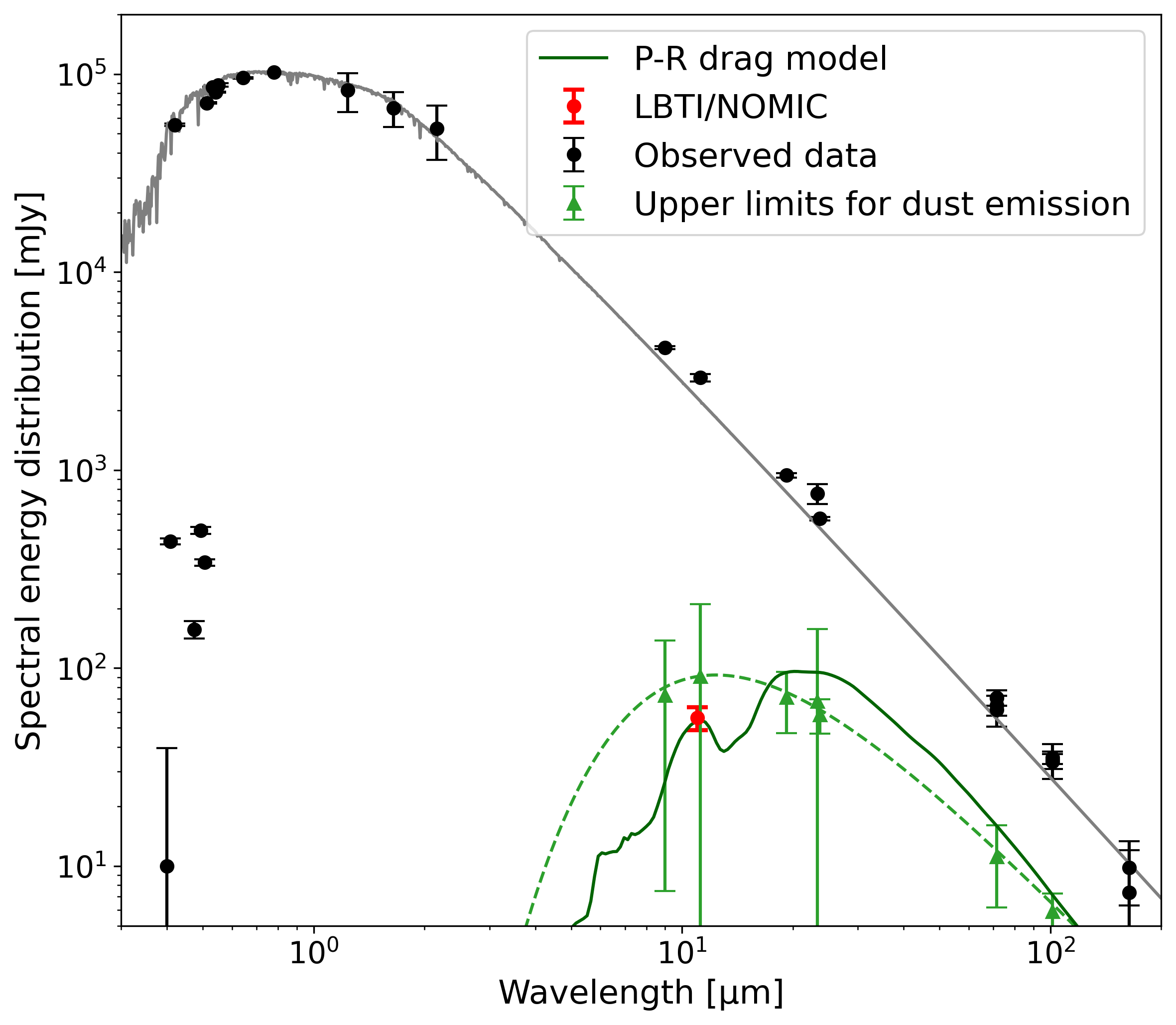
Figure 14: Left: radial distribution of the dust surface brightness models for the combined 2017/2018/2023 dataset. The models are calculated at 11 µm wavelength and their 1$\sigma$ error bars are computed from the MCMC posteriors. The continuous line represents the predicted surface brightness from the P-R drag model, for an outer belt extending from 6 au to 9 au with a mass of $7\times 10^{-6}\,M_{\oplus}$. The dust composition is considered to be 1/3 silicate and 2/3 carbon. Right: SED of the dust from the P-R drag model.

P-R drag hypothesis

One of the main hypothesis to explain the presence of warm exozodiacal dust is the P-R drag mechanism. In such a scenario, dust is formed by planetesimal collisions in an outer belt located further out in the system, and is dragged into the inner region by interaction with stellar radiation before evaporating when reaching sublimation temperature. To simulate this phenomenon, we apply the model presented in Rigley & Wyatt (2020) to the $\theta$ Boo system. In this analytical model, the stellar parameters and the radius of the outer belt are used as input parameters to predict the size distribution of particles in the disk. The size distribution is first simulated in the outer belt using the method in Wyatt et al. (2011). Each dust particle is then assumed to evolve independently inwards, until the system reaches a steady state where the optical depth distribution changes by less than 1 % in a logarithmic time step. The smallest grains that dominate the optical depth typically reach that state after $\sim$10 Myr. The radial profile for each particle is given by the approach in Wyatt (2005). The model then calculates the two-dimensional optical depth distribution over the particle size and the distance from the star. The model finally changes the breadth and mass of the outer belt to fit the surface brightness model from the observation. For determining the emission from the grains in the modeled disk, we again assume the optical properties used to simulate their SEDs in Sec. 6.1.

However, the simulations from this model are only applicable to a system in a steady state within yearly timescales. Indeed, the time for dust particles of blow-out size to drift from 8 au to 2 au is estimated at 35,000 yrs (Wyatt & Whipple, 1950; Burns et al., 1979). This P-R drag model was therefore compared with the model of the combined observing nights of the LBTI (Fig. 8) using a “disk” geometry. The “wide ring” and “thin ring” geometries are indeed not compatible with P-R drag only, and require the presence of a massive object (e.g., a giant exoplanet) to carve their edges. Figure 14 shows the result of the P-R drag model with the best fit surface brightness profile and its corresponding SED. The result is obtained for an outer belt extending from 6 to 9 au, with a mass of $7\times 10^{-6}\,M_{\oplus}$ – considering all the dust particles with a size $\leq 1$ cm. We find that P-R drag can explain our model, with a discrepancy appearing only for $<1$ au separations. However, the outer belt needed to explain this distribution shows an infrared excess that is above the upper limits in Fig. 1 around 25 µm. This suggests that such an outer belt should have been detected by Spitzer.

Since the steady state hypothesis is also not favored by our models (Sec. 5.3), we conclude that other phenomena are likely to influence the dust distribution and generate a yearly variability.

Extreme debris disk hypothesis

The models from Sec. 5 indicate a tentative variability of the exozodiacal disk around $\theta$ Boo, both in its spatial distribution and brightness. Photometric variability of warm dust on monthly to yearly time-scales has already been reported for extreme debris disks (EDDs, Balog et al., 2009). These disks are detected around FGK-type main-sequence stars, and for ages between $\sim$100 to $\sim$200 Myr (Melis et al., 2012; Meng et al., 2012, 2015; Rieke et al., 2021; Moór et al., 2022), and even $>1$ Gyr (Thompson et al., 2019). This variability is commonly thought to originate from major collisions of planetesimals during the terrestrial planet formation phase (Su et al., 2019). Balog et al. (2009) also define EDDs as systems with a total emission at least higher than four times the stellar photospheric output at 24 µm. In the case of $\theta$ Boo, the age of the system is estimated to be 3-4.7 Gyr (Sec. 4), which is well after the terrestrial planet formation phase. Upper limits also indicate that no dust emission higher than a tenth of the stellar photosphere has been detected at 24 µm. This depreciates the hypothesis of an EDD for $\theta$ Boo, with massive planetesimal collisions as the source of the dust and its variations.

Catastrophic event hypothesis

An alternative hypothesis to explain this variability is the consequence of a catastrophic event (massive collision, fragmentation of a massive comet, or passing of a massive object with highly eccentric orbit) that would have occurred in the inner region. After a few years, such an event could generate new dust or disrupt the dust distribution, which would cause an observed brightness variability. For example, some remains of a planet collision happening at 2 au would have a circular orbit of 2.5 years around $\theta$ Boo. After 5 years, the remains would start to form a belt in the HZ that would be detected by the LBTI. While, direct imaging observations in the H- and L-band could not detect the presence of giant planets with masses lower than 11 $M_{\text{Jup}}$. An eccentric planet could indeed disrupt a potential outer belt, and periodically scatter exocomets inwards (Faramaz et al., 2017). From the increase of optical depth in our models, we can estimate the additional mass of material needed to explain it. This material could come from a massive collision or comet fragmentation. For 3 µm grain size, it goes from $10^{-3}\,M_{\text{Vesta}}$ ($4\times 10^{-8}\,M_{\oplus}$) for our “disk” models, to $3\times 10^{-3}\,M_{\text{Vesta}}$ ($1.2\times 10^{-7}\,M_{\oplus}$) for our “wide ring” models. For 10 µm grain size, the estimated mass is tripled.

7 Summary

The HOSTS survey (Ertel et al., 2020) was able to demonstrate a correlation between the presence of cold outer dust and exozodiacal dust. $\theta$ Boo is one of the three exceptions where exozodiacal dust has been detected by the LBTI without prior observations of significant mid- to far-infrared excess emission. In this study, we analyze a multi-epoch observation of the exozodiacal disk around $\theta$ Boo with nulling interferometry at the LBTI in the N’-band. Three observations were taken in UT 2017 April 11, UT 2018 May 23, and UT 2023 May 25 respectively. The data were reduced using the nulling pipeline of the LBTI and analyzed with a model dedicated for exozodiacal disk observations with the LBTI (Kennedy et al., 2015).

A prior assumption for our modeling procedure is to assume that the planetary system of $\theta$ Boo is close to face-on (i.e., $i\sim 0\degree$). This is supported by our extended nulling observation in 2023, which shows no significant relation between the detected emission and the parallactic angle. However, calculations of the stellar inclination indicate that $\theta$ Boo is likely to be edge-on (i.e., $i\sim 90\degree$). To also be edge-on, the exozodiacal disk would thus have to be puffy or diffused. Since our modeling tool can only simulate a vertically thin disk, the assumption of a face-on disk is kept within the scope of this work. The results and conclusions we draw in this study are thus highly dependent on this assumption, and future observations are necessary to constrain the system’s inclination with a higher confidence.

From the models that are obtained for the individual and combined 2017, 2018, and 2023 datasets, we propose different spatial distributions of the dust that can explain our observations. The models for the combined nights are fitting less our data than the models for the individual nights, which favors the hypothesis of an unsteady state system. The different geometries of dust distribution are fitting each night similarly, we are therefore not able to discriminate between them with the LBTI observations. From the Spitzer (2004) and Herschel (2010) observations, we use their obtained upper limits on dust excess emission in the mid- to far-infrared to constrain further the dust distribution. Although our simulated SEDs are still not able to clearly discriminate between the different geometries, they favor a representative size distribution of 3-5 µm for the dust grains.

Using our models for the dust spatial distribution of 2017 and 2023, we are also able to estimate the zodi level and its variability at the EEID. When considering our “disk” models, with a broad distribution of dust in the orbital plane, and for dust grains behaving as ideal blackbodies, we estimate the dust brightness to be $158^{+62}_{-67}$ and $443^{+98}_{-170}$ zodis for 2017 and 2023, respectively. Considering the probability distribution of the two values, we find a tentative increase of dust emission with 1.86$\sigma$ certainty at the EEID. This result hints at a possible brightness variability of exozodiacal disks in the HZ of main-sequence stars. More observations are needed in the future to confirm this trend for $\theta$ Boo. The obtained zodi levels are, however, dependent on the chosen dust temperature, and hence on the size distribution of the dust grains. For realistic grains with a size of 3 µm for example, the obtained zodi levels are $63^{+24}_{-26}$ and $173^{+39}_{-67}$ zodis for 2017 and 2023, respectively. More constraints on the dust properties are therefore necessary to estimate the absolute zodi level of the system.

Several hypotheses are considered for the origin of the exozodiacal dust and its variability: (1) the P-R drag, (2) the EDD, and (3) the catastrophic event. The first hypothesis, P-R drag, is one of the main mechanism to explain the presence of warm dust, continuously generated by a collisionally active asteroid belt analogue. However, non-detections of far-infrared excess limit the prominence of such a belt. Using our steady state model, with the combined 2017/2018/2023 nights, we are able to retrieve the dust distribution from P-R drag for an outer parent belt extending from 6 au to 9 au with a mass of $7\times 10^{-6}\,M_{\oplus}$. However, since our steady state model is not favored, another mechanism is likely to influence the dust distribution besides P-R drag, and generate a yearly variability.

The second hypothesis, considering an EDD, could explain the variability but is unlikely considering the age of $\theta$ Boo and the level of excess infrared emission from the dust. The third hypothesis is the consequence of a catastrophic event (massive collision, fragmentation of a massive comet, or passing of a massive object with highly eccentric orbit). We estimate the amount of additional material injected in the system to explain this variability. Considering dust particles from 3 µm to 10 µm, and for our different model geometries, we find an additional mass of $10^{-3}-10^{-2}\,M_{\text{Vesta}}$ ($M_{\text{Vesta}}\simeq 4\times 10^{-5}\,M_{\oplus}$). The presence of a substellar companion that could disrupt the dust distribution has also been constrained using high-contrast AO observations in the H- and L’-bands with the SHARK-NIR and LMIRCam instruments, respectively. These observations were performed on UT 2024 February 24, but did not show any features indicating the presence of a point-like companion source in the system. Nonetheless, the contrast limits of the images enabled us to constrain the presence of giant planets down to 11 $M_{\text{Jup}}$ at 1.3″ angular separation, based on a “hot start” evolutionary model.

To overcome the currently faced challenges when studying the exozodiacal disk of $\theta$ Boo, more observations will be needed. In particular, detections at different wavelengths in the mid-infrared (e.g., using the JWST/MIRI instrument) would help constraining further the dust properties and its temperature profile. More sensitive observations in the far-infrared would also search for emissions from a cold outer debris disk that could feed the warm dust, and hint us to the system’s orientation. More LBTI observations with reduced noise would also enable a more precise modeling of the distribution and orientation of the warm dust, especially by considering the dependence of the null measurements with the parallactic angle. Implementation of the PCA method for background subtraction (Rousseau et al., 2024), and the upcoming new detector for NOMIC should reduce the instrumental noise and improve future observations.

Appendix A Null depths

Figure 15: Nulls with respect to UT (left) and parallactic angle (right) for 8 pixels aperture radius. (top) 2017 April 11, (middle) 2018 May 23, (bottom) 2023 May 25.

Figure 16: Nulls with respect to UT (left) and parallactic angle (right) for 16 pixels aperture radius. (top) 2017 April 11, (middle) 2018 May 23, (bottom) 2023 May 25.

Figure 17: Nulls with respect to UT (left) and parallactic angle (right) for 24 pixels aperture radius. (top) 2017 April 11, (middle) 2018 May 23, (bottom) 2023 May 25.

Figure 18: Nulls with respect to UT (left) and parallactic angle (right) for 32 pixels aperture radius. (top) 2017 April 11, (middle) 2018 May 23, (bottom) 2023 May 25.

Figure 19: Nulls with respect to UT (left) and parallactic angle (right) for 40 pixels aperture radius. (top) 2017 April 11, (middle) 2018 May 23, (bottom) 2023 May 25.

Appendix B Corner plots

Figure 20: Corner plots showing the MCMC posteriors for the model fitting of the 2017 (left) and 2018 (right) datasets. The posteriors are given for a “disk” (top), “wide ring” (middle), and “thin ring” (bottom) geometry.

Figure 21: Corner plots showing the MCMC posteriors for the model fitting of the 2023 (left) and the combined 2017/2018/2023 (right) datasets. The posteriors are given for a “disk” (top), “wide ring” (middle), and “thin ring” (bottom) geometry.