Personalized Federated Learning under Model Dissimilarity Constraints

Abstract

One of the defining challenges in federated learning is that of statistical heterogeneity among clients. We address this problem with Karula, a regularized strategy for personalized federated learning that constrains the pairwise model dissimilarities between clients based on the difference in their distributions. Model similarity is measured using a surrogate for the 1-Wasserstein distance adapted for the federated setting, allowing the strategy to adapt to highly complex interrelations between clients that, e.g., clustered approaches fail to capture. We propose an inexact projected stochastic gradient algorithm to solve the resulting constrained optimization problem, and show theoretically that it converges as $O(1/K)$ to the neighborhood of a stationary point of a smooth, possibly non-convex, loss. We demonstrate the effectiveness of Karula on synthetic and real federated data sets.

1 Introduction

Federated learning (FL) is a paradigm for training models on decentralized data that remains with clients in a network coordinated by a central server. Developed in response to the growing prevalence of private, decentralized data sources—such as mobile devices and hospital databases—FL enables collaborative and communication-efficient model training without requiring the exchange of client data. One example of an FL algorithm is Federated averaging (McMahan et al.,, 2017) where clients perform local gradient steps on a global model and send updated model parameters to the server. The server then averages these and returns the updated global model to the clients. There are many examples where FL has been applied successfully, leading to greater communication-efficiency and data privacy, e.g., in mobile keyboard prediction (Hard et al.,, 2018), autonomous driving (Nguyen et al.,, 2022), and healthcare (Qayyum et al.,, 2022). However, FL faces several challenges that arise due to client heterogeneity, be it in terms of models, hardware, or data. In the case of data heterogeneity, the client data follow different statistical distributions and may have varying number of observations. This means that the performance of standard FL systems, which learn a single global model, can suffer significantly in terms of both convergence and generalization. At the same time, due to limited data, non-collaboratively training separate models also leads to poor generalization.

Therefore, in settings where data heterogeneity is significant, federated learning systems should ideally learn personalized models that borrow strength from others while respecting local nuances in their data. Personalized federated learning (PFL) strategies aim to accomplish this through two primary approaches: (1) globally anchored personalization, where local models leverage knowledge from a central global model; and (2) peer-based personalization, where local models learn from similar clients identified at the server level. Globally anchored strategies are appropriate in applications where we expect each client to have limited dissimilarity with any other client in the network, such as in next-word prediction on mobile devices. However, in applications such as recommender systems, distributional differences between two given clients can be very large. Peer-based methods address this issue by attempting to only learn from clients that are similar. One approach to peer-based personalization is to cluster clients, prior to training or concurrently. The cluster model of statistical heterogeneity does however fail to capture more complex overlaps between clients. As an example, in a music recommendation application, suppose one user (client) is only interested in jazz and classical, another in jazz and funk, and yet another in funk and rock. Clearly, no hard clustering of these users will capture these relationships accurately. Other approaches to peer-based personalization allow for more complex relationships between the local models of clients, but to the best of our knowledge no prior work incorporates distributional similarity measures in a principled manner.

Motivated by this, we develop a PFL strategy that uses approximations of the Wasserstein distance to measure distributional similarity between clients, and in turn, leverages similarity by constraining the dissimilarities between the personalized models. Our method approximates the Wasserstein distances in a manner that does not necessitate the exchanging of client data.

1.1 Contributions

The main contributions of this work are threefold:

• We propose a peer-based PFL strategy that learns personalized models that are centerally constrained to have limited pairwise dissimilarity. These constraints are derived in a principled, fully data-driven manner using approximations of the Wasserstein distances between empirical client distributions. This design is grounded in theoretical insights developed in this work.

• We develop an efficient inexact projected stochastic gradient method tailored to our framework. It employs variance reduction to deal with partial client participation in each communication round. Due to this variance reduction, we are able to show convergence for smooth, possibly non-convex losses at rate $O(1/K)$ to an $\epsilon$-stationary set of personalized models, where the error $\epsilon$ arises only due to stochastic gradients from the clients and inexact projection at the server level.

• We evaluate our approach on both synthetic and real-world heterogeneous datasets across regression and classification tasks. Our method is compared against a variety of standard federated and personalized FL baselines, demonstrating several distinctive advantages.

1.2 Outline

In §2 we describe some of the related work, relating our contribution to existing literature. Then, in §3, we introduce our proposed strategy for personalized federated learning, which is followed by a convergence analysis in §4. Numerical experiments validate our proposed method in §5. We conclude the paper by summarizing and discussing our findings in §6.

2 Related work

Statistical heterogeneity presents significant challenges to both traditional and distributed learning systems, affecting inference and generalization. It arises in various applications where data can be assumed to be drawn from distinct distributions. For example, in meta-analysis, studies with participants from different populations are aggregated (Melsen et al.,, 2014); in medicine, different clinical features in patients affect individual health outcomes (Machado et al.,, 2011); and in finance, markets adopt different regimes over time (Ang and Timmermann,, 2012). In the context of FL, the statistical heterogeneity among clients is generally considered one of the defining aspects of the field. Zhao et al., (2018) and Karimireddy et al., (2020) show that both convergence and generalization of conventional FL algorithms are severely affected by statistical heterogeneity. The heterogeneity introduces difficulties in optimizing the global model, as local updates cause models to drift, reducing the effectiveness of aggregation methods and slowing down convergence. The former work shows that the 1-Wasserstein distance between client distributions can be used to quantify this effect.

One approach to address the challenges caused by statistical heterogeneity is stratification, whereby different models are fit for every value of some categorical parameter, which are assumed to correspond to the different underlying distributions. Stratified models allow each subgroup to be modeled independently, capturing the unique characteristics of each distribution and reducing the bias that arise from pooling heterogeneous data. In clinical trials, it is common to do this by grouping participants into different strata based on relevant clinical features, and fitting a model for each strata (Kernan et al.,, 1999). Stratification does, however, reduce the number of observations for each model, limiting the viability of naive stratification in many settings. PFL models, which adapt to individual clients rather than enforce a single global model, are a special case of stratified models where the stratification is performed at the level of individual clients.

Globally anchored personalization.

A common approach to PFL is to learn local models that are, in some sense, close to a shared global model. Fallah et al., (2020) take this approach using meta-learning to formulate a method that learns a global model, from which each client takes a few local gradient descent steps to produce the local model. Additionally, they show a connection between the convergence of their method and the statistical heterogeneity measured in total variation and Wasserstein distance, respectively. Taking a regularization approach to the problem, the works of Dinh et al., (2020) and Li et al., (2021) propose methods that penalize the squared norm difference between the local and the global model. Yet another approach is given by Deng et al., (2020), whose algorithm learns personalized models that are convex combinations of a shared global model and a completely local model.

Peer-based personalization.

A more flexible personalization strategy is to identify clients that are similar and borrow strength from them directly rather than from a single aggregated model. One way to do this is by clustering the clients. The PFL method proposed by Ghosh et al., (2020) does this iteratively by alternating between optimizing the cluster models and clustering the clients, which is done by finding the cluster whose model achieves the smallest local loss. Regularized methods for peer-based PFL include convex clustering via a group-lasso penalty on the differences of models (Armacki et al.,, 2022) and Laplacian regularization (Dinh et al.,, 2022; Hashemi et al.,, 2024). The empirical results of Dinh et al., show that in fact Laplacian regularization with randomized weights outperform globally anchored personalization strategies on many tasks.

Similarity measures.

Measures of task and distribution similarity are of great interest in several learning contexts, particularly transfer learning (Zhong et al.,, 2018; Pan,, 2020), multi-task learning (Shui et al.,, 2019), and meta-learning (Zhou et al.,, 2021). These measures quantify how closely related different tasks or data distributions are, influencing decisions on model adaptation, aggregation, and generalization. Common approaches include statistical distance metrics such as the Kullback-Leibler divergence (Kullback and Leibler,, 1951), Jensen-Shannon divergence (Lin,, 1991), and Wasserstein distance (Kantorovich,, 1960). In addition, similarity can be assessed through feature-space representations using methods like cosine similarity or kernel-based measures.

3 Proposed method

In this section, we introduce Karula, a strategy for federated learning of personalized models where model differences are constrained by the distributional similarity of client data. This reinforces the intuitive notion that clients with similar data should learn similar models. We also propose an efficient projected stochastic gradient method with variance reduction to handle partial client participation during communication rounds. This method is also suitable for use in other FL strategies.

3.1 Main idea

Consider an FL setting with $N$ clients, each able to communicate with a central server. To each client $i\in\{1,\dots,n\}$, we associate an underlying distribution $\mu_{i}\colon 2^{\mathcal{X}}\to{\mbox{\bf R}}_{+}$, where $\mathcal{X}$ is the feature space. Each client holds a dataset $\mathcal{D}_{i}$ of $N_{i}$ independent samples drawn from $\mu_{i}$. The learning goal is to find a personalized model $\theta_{i}\in\Theta$ for each client that minimizes their expected loss $f_{i}(\theta_{i})={\mathbbmss{E}}_{\xi\sim\mu_{i}}[\ell(\theta_{i},\xi)]$, where $\ell\colon\Theta\times\mathcal{X}\to{\mbox{\bf R}}$ is a loss function, and $\Theta$ is the parameter space. However, due to limited available data on each client, attempting to directly minimize $f_{i}(\theta_{i})$ leads to poor generalization. To address this challenge, we introduce a regularization strategy that couples the learning tasks across clients by approximately solving a constrained optimization problem:

$$\begin{array}[]{ll}\underset{\theta_{i}\in\Theta}{\mbox{minimize}}&\frac{1}{n}\sum_{i=1}^{n}\alpha_{i}f_{i}(\theta_{i})\\ \mbox{subject to}&\|\theta_{i}-\theta_{j}\|_{2}^{2}\leq tD_{ij},\quad i,j\in\{1,\dots,n\}.\end{array}$$ (1)

Here $t\geq 0$ is a regularization parameter, each $\alpha_{i}$ is a positive weight, and each $D_{ij}\geq 0$ is a dissimilarity parameter which quantifies the dissimilarity between clients $i$ and $j$ that is calculated before solving the minimization problem. This formulation generalizes the standard FL formulation, since by selecting $t=0$ the problem is equivalent to choosing a single global model that minimizes the average loss. In the other extreme, when $t\to\infty$, we obtain completely local models except for clients that are deemed to have identical distributions, i.e., when $D_{ij}=0$. In the sequel, we show how to choose the similarity parameters in a completely data-driven manner, based on a surrogate for the Wasserstein distance.

3.2 Model dissimilarity and Wasserstein distance

To quantify the relationship between data distributions and the corresponding learned models, we consider the 1-Wasserstein distance—also known as the earth mover’s distance or the Kantorovich–Rubinstein distance. Suppose the data space $\mathcal{X}$ is equipped with a metric $d_{\mathcal{X}}$. The 1-Wasserstein distance between two distributions $\mu_{i}$ and $\mu_{j}$ is defined as

$$W_{1}(\mu_{i},\mu_{j})=\inf_{\pi\in\Pi(\mu_{i},\mu_{j})}{\mathbbmss{E}}_{(\xi,\xi^{\prime})\sim\pi}[d_{\mathcal{X}}(\xi,\xi^{\prime})],$$

where $\Pi(\mu_{i},\mu_{j})$ is the set of all probability measures with marginals $\mu_{i}$ and $\mu_{j}$. This distance is a proper metric on the space of distributions on $\mathcal{X}$, satisfying symmetry, positive definiteness, and the triangle inequality (Villani,, 2008).

We will now show that under two mild conditions, the dissimilarities of the ideal models for two distributions can be bounded by the 1-Wasserstein distance. The first assumption is that the losses grow at a quadratic rate when diverting from the ideal model. This condition is satisfied by all losses whose convex envelopes are strongly convex. The second assumption is that the loss function is Lipschitz continuous with respect to the data, i.e., a small difference between two samples imply a small difference in the value of the loss function $\ell$ at any given model parameters.

Assumption 3.1.

The loss functions $f_{i}$ have quadratic functional growth with parameter $\gamma>0$, meaning for the ideal model $\theta_{i}^{\star}=\operatornamewithlimits{argmin}_{\theta_{i}}f_{i}(\theta_{i})$, the bound $f_{i}(\theta_{i})-f_{i}(\theta_{i}^{\star})\geq(\gamma/2)\|\theta_{i}-\theta_{i}^{\star}\|^{2}$ holds for every $\theta_{i}\in\Theta$.

Assumption 3.2.

The loss function $\ell$ is $L_{\mathcal{X}}$-Lipschitz continuous in its second argument with respect to the metric $d_{\mathcal{X}}$, meaning $|\ell(\theta,\xi)-\ell(\theta,\xi^{\prime})|\leq L_{\mathcal{X}}d_{\mathcal{X}}(\xi,\xi^{\prime})$ for every $\theta\in\Theta$.

Remark 3.3.

The latter assumption holds naturally for some loss functions, but for others, e.g. linear regression with quadratic loss, we need to require $\Theta$ to be bounded.

Proposition 3.4.

Suppose Assumptions 3.1 and 3.2 hold. Then the ideal models satisfy

$$\|\theta_{i}^{\star}-\theta_{j}^{\star}\|_{2}^{2}\leq\frac{2L_{\mathcal{X}}}{\gamma}W_{1}(\mu_{i},\mu_{j}).$$ (2)

Proof.

The proof of this result, and all forthcoming results, is presented in Appendix A. ∎

Why not estimate model dissimilarity directly?

A straight-forward approach to shrink the model dissimilarities would be to learn completely local models first, calculate their pairwise distances, and then use them as the dissimilarity parameters. So why use a less direct approach with Wasserstein distances? In the FL setting, it is common for clients to have more features than observations. For instance, in a linear regression task with $d$ important features and $N$ observations per client, it is well known that the minimax squared estimation error is $O(d/N)$ (Bickel et al.,, 2009; Raskutti et al.,, 2011). When $N<d$, no meaningful upper bound on the estimation error can be guaranteed without additional structural assumptions. The situation worsens for overparameterized models, where the number of parameters exceeds the number of features. In contrast, the Wasserstein distance between two empirical distributions has a rate of $O(N^{-1/d})$ (Wang et al.,, 2021, Example 1). While this rate is very slow in high dimensions, it clearly performs much better than $O(d/N)$ when $N$ is on a similar scale as $d$, or is smaller. We show empirically in §5.1 how our approach is better at estimating the true dissimilarities.

Choosing the data metric.

In supervised learning, a natural way to define the data metric $d_{\mathcal{X}}$ is to concatenate the feature vector and response, and apply a standard norm—such as the Euclidean distance—on the joint space. An alternative approach, proposed by Elhussein and Gursoy, (2024), combines cosine similarity for the features with the Hellinger distance for the responses. They argue that cosine-similarity is more informative in high-dimensional feature spaces due to the concentration of measures phenomenon, and that the Hellinger distance compares densities within their statistical manifold, potentially yielding more meaningful distinctions between distributions.

Calculating the dissimilarity parameters.

With the present motivation in mind, it is natural to set the dissimilarity parameters proportional to the Wasserstein distance between the empirical distributions, $W_{1}(\hat{\mu}_{i},\hat{\mu}_{j})$, where $\hat{\mu}_{i}$ is the empirical distribution of client $i$th. While Rakotomamonjy et al., (2023) propose an iterative method to approximate these distances in a federated manner, their approach requires computing $n(n-1)/2$ optimal transport plans per iteration—an operation that is computation and communication-intensive.

To reduce this cost, we propose to approximate the Wasserstein distances via linear embedding of the data sets, following prior work such as Kolouri et al., (2020) and Liu et al., (2025). Specifically, we introduce a reference data set of $N_{0}$ independent samples $\mathcal{D}_{0}=\{\xi_{1}^{0},\dots,\xi_{N_{0}}^{0}\}$ drawn from a reference distribution $\mu_{0}$. The optimal transport plan between the empirical distributions $\hat{\mu}_{0}$ and $\hat{\mu}_{i}$ is then

$$\pi_{i}^{\star}=\operatornamewithlimits{argmin}_{\pi\in\Pi(\hat{\mu}_{0},\hat{\mu}_{i})}\sum_{j=1}^{N_{0}}\sum_{k=1}^{N_{i}}\pi_{jk}d_{\mathcal{X}}(\xi_{j}^{0},\xi_{k}^{i}).$$

By approximating the Monge map via $M_{i}=N_{0}\pi_{i}^{\star}\mathcal{D}_{i}$, we can define an embedding $\Phi$ by $\Phi(\mathcal{D}_{i})=(M_{i}-\mathcal{D}_{0})/\sqrt{N_{0}}$ that has the property that $\|\Phi(\mathcal{D}_{i})-\Phi(\mathcal{D}_{j})\|_{1}$ defines a metric on the space of data sets, and indeed approximates the Wasserstein distance $W_{1}(\hat{\mu}_{i},\hat{\mu}_{j})$. We thus choose the dissimilarity parameters as $D_{ij}=\|\Phi(\mathcal{D}_{i})-\Phi(\mathcal{D}_{j})\|_{1}$. By doing this, each client only has to compute a single optimal transport plan. Also, on the communication side, only a reference data set and the embeddings need to be transmitted over the network once, totaling $O(N_{0}dn)$ communication.

3.3 Algorithm

To solve the Karula problem (1), we introduce a projected gradient algorithm that supports partial client participation in each training round. To eliminate the error introduced by this partial participation, our algorithm uses variance reduction, taking inspiration from methods such as Saga (Defazio et al.,, 2014) and Fedvarp (Jhunjhunwala et al.,, 2022). Our approach can be viewed as a relaxation of standard distributed stochastic gradient method: rather than enforcing full mode agreement, each iteration shrinks model dissimilarities based on pairwise constraints. Specifically, we consider the following formulation of the Karula problem (1):

$$\begin{array}[]{ll}\underset{\theta\in\mathcal{K}}{\mbox{minimize}}&f(\theta)=\frac{1}{n}\sum_{i=1}^{n}\alpha_{i}f_{i}(\theta_{i}),\quad\mathcal{K}=\{\theta\in\Theta^{n}\colon\|\theta_{i}-\theta_{j}\|^{2}\leq tD_{ij}\}.\end{array}$$

Each client $i$ serves as a stochastic first-order oracle $G_{i}$ that returns a stochastic gradient when queried with a model $\theta_{i}$. Based on this formulation, we apply the stochastic projected gradient method outlined in Algorithm 1. In each training round, a subset of clients returns stochastic gradients to the server, which then performs a variance reduced gradient step with respect to $f$, and approximately projects the iterate onto the constraint set $\mathcal{K}$.

The projection $\Pi_{\mathcal{K}}(\vartheta)$ of a collection of models $\vartheta\in\Theta^{n}$ onto $\mathcal{K}$ does not admit an analytical solution, so we use an iterative method to approximate it. To this end, we define the $\delta$-inexact projection $\Pi_{\mathcal{K}}^{\delta}\colon\Theta^{n}\to\mathcal{K}$ that returns a feasible collection of models $\theta=\Pi_{\mathcal{K}}^{\delta}(\vartheta)$ which is at most $\delta$-suboptimal in the projection problem, meaning

$$\frac{1}{2\eta}\|\theta-\vartheta\|^{2}\leq\delta+\frac{1}{2\eta}\min_{v\in\mathcal{K}}\|v-\theta\|^{2}$$

for the learning rate $\eta>0$. We describe how to perform the projection computation in the supplemental material.

Algorithm 1 Karula

 Setup: Initializations $(\phi_{1}^{0},\dots,\phi_{n}^{0})$, step size $\eta$, participation size $s$, number of iterations $K$.

 Server receives initializations $\phi_{i}^{0}$ and stochastic gradients $G_{i}(\phi_{i}^{0})$ from clients $i\in\{1,\dots,n\}$, and forms $\theta^{0}=(\phi_{1}^{0},\dots,\phi_{n}^{0})$ and $g^{0}=(G_{1}(\phi_{1}^{0}),\dots,G_{n}(\phi_{n}^{0}))/n$.

 for $k=0,\dots,K-1$ do

  Server samples uniformly a subset $S_{k}\subset\{1,\dots,n\}$ of $s$ clients and sends $\theta_{i}^{k}$ to client $i\in S_{k}$.

  Client $i\in\{1,\dots,n\}$ updates

$$\phi_{i}^{k+1}=\begin{cases}\theta_{i}^{k}&\text{if }i\in S_{k},\\ \phi_{i}^{k}&\text{otherwise}.\end{cases}$$

  Client $i\in S_{k}$ returns $G_{i}(\phi_{i}^{k+1})$ to the server.

  Server sets

$$g_{i}^{k+1}=\begin{cases}G_{i}(\phi_{i}^{k+1})&\text{if }i\in S_{k},\\ g_{i}^{k}&\text{otherwise}.\end{cases}$$

and updates $\nu^{k}=g^{k}+(g^{k+1}-g^{k})/s$.

  Server performs inexact projected gradient step $\theta^{k+1}=\Pi_{\mathcal{K}}^{\delta}(\theta^{k}-\eta\nu^{k})$.

 end for

4 Convergence analysis

In this section, we analyze the convergence properties of our proposed algorithm for solving Problem (1), both in the general smooth case when the losses have Lipschitz continuous gradients. The analysis is inspired by the work of Reddi et al., (2016), which we have adapted for the FL setting, and extended to allow for inexact projections and stochastic gradients of the individual client losses $f_{i}$.

Our goal in the smooth, possibly nonconvex case, is to find a local minimizer, but since the problem is constrained, the ordinary stationarity condition $0=\nabla f(\theta)$ is not appropriate. In lieu, the analogous condition for constrained optimization is that $\theta$ is a zero of the gradient mapping (cf. Nesterov,, 2018)

$$\mathbf{G}_{\eta}(\theta)=\frac{1}{\eta}\left(\theta-\Pi_{\mathcal{K}}(\theta-\eta\nabla f(\theta)\right).$$

Informally, we can think of the condition $0=\mathbf{G}_{\eta}(\theta)$ as saying one of two things: either $\theta$ is a feasible point with zero gradient, or it is a point such that the negative gradient is normal to the feasible set.

To establish the convergence results, we make a few standard assumptions. First, we assume smoothness of the losses.

Assumption 4.1.

The weighted losses $\alpha_{i}f_{i}$ are $L$-smooth, i.e.they are continuously differentiable with $L$-Lipschitz continuous gradients: $\alpha_{i}\|\nabla f_{i}(\theta_{i})-\nabla f_{i}(\theta_{i}^{\prime})\|\leq L\|\theta_{i}-\theta_{i}^{\prime}\|$ for all $\theta_{i}$ and $\theta_{i}^{\prime}$.

Second, we assume that the stochastic gradients have bounded mean squared error.

Assumption 4.2.

The stochastic gradients returned by the oracles $G_{i}$ have bounded mean squared error: ${\mathbbmss{E}}\|G_{i}(\theta_{i})-\alpha_{i}\nabla f_{i}(\theta_{i})\|^{2}\leq\sigma^{2}$ for every $\theta_{i}$.

Under the two former assumptions, the proposed algorithm enjoys sublinear convergence to an $\epsilon$-stationary point where $\epsilon$ reflects the effect of stochastic gradients and inexact projections. Here, we assume feasible initialization only for the sake of exposition, which is trivially satisfied by assigning the same initial model to all clients.

Theorem 4.3.

Under Assumptions 4.1 and 4.2, with feasible initialization, step size $\eta=3/(8L)$ and $2\leq s\leq n-1$, the iterates of Algorithm 1 satisfy

$$\min_{k=0,\dots,K-1}{\mathbbmss{E}}\|\mathbf{G}_{\eta}(\theta^{k})\|^{2}\leq\frac{8L}{3}\left(\frac{f(\theta^{0})-f(\theta^{\star})}{K}+\epsilon\right),$$

where $\epsilon=4\sigma^{2}(s+1)/s+2\delta$.

Remark 4.4.

In contrast to many other FL algorithms, our convergence analysis does not require any bounds on client heterogeneity or assumptions about the underlying data distributions. Instead, it only relies on standard machine learning assumptions. Moreover, the step size that is used to achieve the bound is comparatively generous, and works well in practice provided that the smoothness constant $L$ is known or can be effectively estimated.

Remark 4.5.

While it is common to assume exact projections in theory, this is not particularly realistic. Our analysis explicitly accounts for projection errors and quantifies how these affect the size of the neighborhood that the algorithm converges to. This has practical implications, since it informs the choice of the error $\delta$ to trade off the iteration cost with proximity to stationarity.

5 Numerical experiments

We are now ready to study the performance of Karula empirically and compare it against several existing conventional and personalized FL strategies. First, in §5.1, we study ridge regression on synthetic, heterogeneous data where the true model parameters are known. Then, in §5.2, we evaluate the performance of the different methods on a federated handwritten digit classification task using neural network models. For simplicity, we use the Euclidean norm on the joint space of the features and labels for the dissimilarity parameter computation. The experiments in §5.1 and §5.2 were performed on an Intel Core i9 processor at 3.2 GHz, and on a cluster with Intel Xeon processors at 3.10 GHz, respectively.

Benchmark strategies.

We compare Karula with three FL baselines: local non-collaborative learning, federated averaging with five local iterations, and IFCA. For all methods and experiments, we weight the client loss functions by the number of local samples.

5.1 Synthetic data

We begin by comparing the performance of the FL strategies on a ridge regression problem with $d=50$ features. The ridge penalty parameter is set to $\lambda=10^{-6}$ to ensure a unique solution. One third of the clients participate at every round, and clients return full gradients.

Data generation.

We simulate a network of $n=30$ clients, where the ground-truth model parameters for a third of the clients are drawn from a normal distribution with mean $1$, another third from a normal distribution with mean $1.5$, and the final third from a normal distribution with mean $2$. Feature matrices are also drawn from distinct normal distributions across the clients. Each client draws $N_{i}$ samples from their assigned distribution, where $N_{i}$ is uniformly distributed between 10 and 100. The noise level is tuned so that the global model outperforms the completely local models.

Hyperparameter selection.

To set a level playing field for the comparison, we use 5-fold cross-validation to select the regularization parameters of IFCA and Karula. While this tuning approach may not always be practical in large-scale FL deployments, it provides a controlled benchmark setting for our experiments. The learning rate $\eta$ is set to $1/(10L)$, $1/(2L)$ and $3/(8L)$ for FedAvg, IFCA and Karula, respectively.

Results.

Table 1 summarizes the results of the synthetic ridge regression experiments, reporting both estimation error and test $R^{2}$. Karula clearly outperforms the baselines, achieving the lowest estimation error and highest predictive performance. While FedAvg and IFCA improve substantially over fully local models, they fail to capture the underlying heterogeneity among clients. In particular, IFCA does not discover meaningful client clusters and effectively collapses to learning a single global model. To better understand this behavior, Figure 1 compares the true pairwise model dissimilarities with the dissimilarity parameters used by Karula and those estimated directly from local models. As shown, the dissimilarity structure inferred by Karula matches the ground truth closely, whereas direct estimation from local models fails to recover the correct relational structure. This result supports our argument from §3.2 that Wasserstein-based approximations provide more reliable measures of client similarity in low-sample regimes.

Table 1: Mean estimation error and test $R^{2}$ of the different strategies on synthetic ridge regression experiment, with $\pm 2\times\text{SE}$.

Strategy	Estimation error	Test $R^{2}$
Local	35.33 $\pm$ 2.729	0.692 $\pm$ 0.108
FedAvg	7.47 $\pm$ 0.493	0.846 $\pm$ 0.026
IFCA	7.69 $\pm$ 0.509	0.821 $\pm$ 0.024
Karula	5.86 $\pm$ 0.204	0.938 $\pm$ 0.009

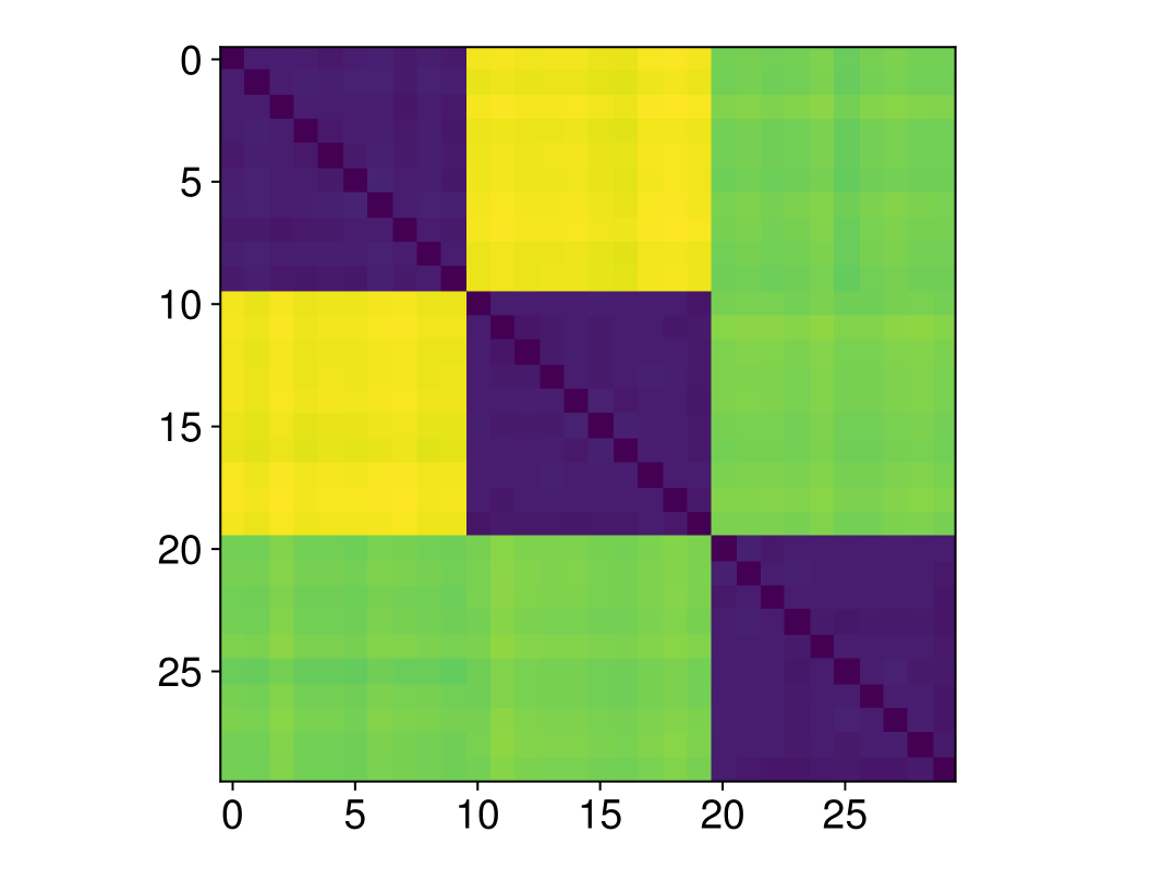
(a) Ground truth

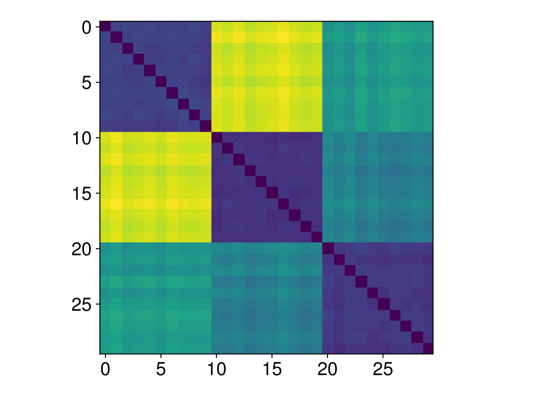
(b) Karula

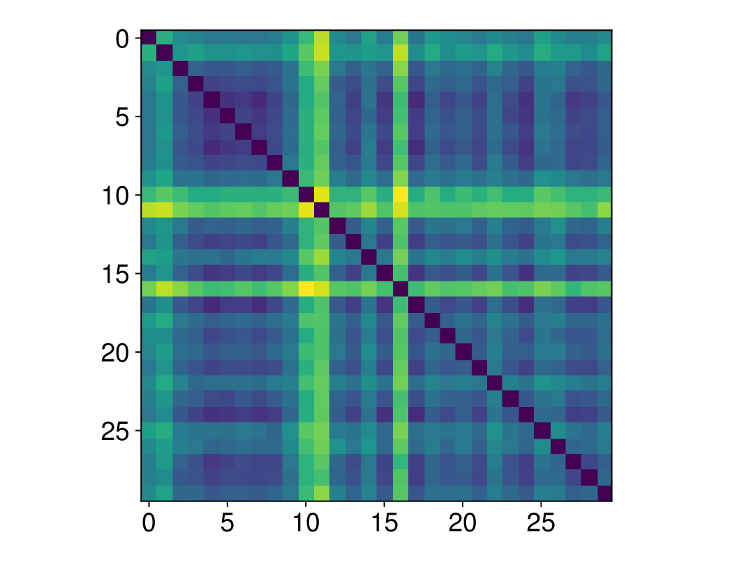
(c) Local

Figure 1: Heatmaps showing the true model dissimilarities, the dissimilarity parameters calculated by Karula, and the model dissimilarities estimated via local learning, respectively.

5.2 Federated MNIST

Next, we run experiments on a federated version of the MNIST dataset (Caldas et al.,, 2019), where the task is to classify handwritten digits $\{0,\dots,9\}$. Each client holds data of handwritten digits corresponding to one individual writer. Here, heterogeneity stems from idiosyncratic handwriting: e.g., some write large, others small; some write “1” with serifs, others write without. We compare the performances of the different strategies on a network of $n=30$ clients, where half of them participate in every round. The clients return minibatch stochastic gradients with a batch size of 64.

Model architecture and personalization.

We use a two-layer perceptron model with ReLU activation and a hidden layer of 100 neurons. Following the personalization strategy in Arivazhagan et al., (2019) and the experimental setup of Ghosh et al., (2020), we apply personalization only to the second (output) layer of the model.

Hyperparameter selection.

For FedAvg and IFCA we use $\eta=10^{-4}$, whereas for the local model and Karula we use $\eta=2\times 10^{-4}$. For IFCA, we specify three clusters (following §6.3 in Ghosh et al.,, 2020). For Karula, the pairwise dissimilarity threshold is set to $t=20$.

Results.

Figure 2 shows the training loss and test performance of the different strategies. The final average test accuracy is 91.3$\pm$0.75% for Karula, 89.3$\pm$0.78% for local learning, 84.4$\pm$2.39% for FedAvg, and 83.9$\pm$2.60%, respectively. Notably, Karula not only yields better average accuracy, but also exhibits lower variance in the results, even though IFCA and FedAvg use smaller learning rates. To illustrate the interpretability of the dissimilarity parameters computed by Karula, Figure 3 visualizes the pairwise relationships among a subset of three clients. We clearly see how the learned dissimilarity structure reflects meaningful variations in the client data distributions, aligning with the underlying differences in handwriting.

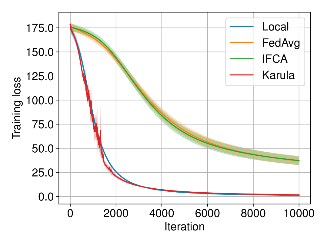
(a) Training loss on federated MNIST.

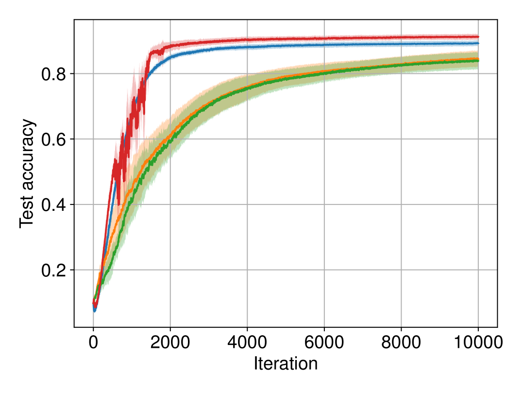
(b) Test accuracy on federated MNIST.

Figure 2: Training and test performance with $\pm 2\times\text{SE}$ bands of FL strategies on classification task with 2NN model on Federated MNIST dataset with $n=30$ clients.

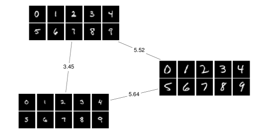
Figure 3: Example handwritten digits from three clients and the dissimilarity parameters $D_{ij}$ between them. The clients were chosen by randomly sampling one, and subsequently finding the nearest and most remote neighbor, respectively.

6 Discussion

We have introduced Karula, a personalized federated learning (PFL) strategy based on constrained optimization and data-driven measures of client dissimilarity. At the core of our approach is a surrogate for the 1-Wasserstein distance between client data distributions, which we compute efficiently via linear embeddings without any exchange of raw client data. This embedding-based dissimilarity offers a scalable and communication-efficient way to capture structural variation across clients. Under mild conditions on the loss functions, we proved that the distance between ideal personalized models can be bounded in terms of the Wasserstein distance between client distributions. This theoretical connection justifies constraining pairwise model dissimilarities as a means of improving generalization. To solve the resulting constrained problem, we proposed a projected stochastic gradient algorithm that supports partial client participation and incorporates variance reduction. We show that the method converges to an $\epsilon$-stationary point under standard assumptions, even for nonconvex losses. Empirical results on both synthetic and real-world federated datasets demonstrate the effectiveness of our approach. On the synthetic task, the learned dissimilarity parameters closely align with the true model distances, leading to superior personalized performance. On the federated MNIST benchmark, we could see that Karula can perform well on a real federated dataset, and that the algorithm converges quickly even when dealing with a nonconvex loss.

Limitations.

The model for communication constraints used in our analysis, although common in the federated learning literature, is not entirely realistic. It ignores the possibility of some clients communicating with the server significantly less often than others. Moreover, our accounting for inexact projections still assumes feasibility of the approximation, which is not always guaranteed in practice.

Appendix A Proofs of results

A.1 Proof of Proposition 3.4

Proof.

Under Assumptions 3.1, the ideal models $\theta_{i}^{\star}$, $i\in\{1,\dots,n\}$, satisfy

$$\frac{\mu}{2}\|\theta_{i}^{\star}-\theta_{j}^{\star}\|^{2} \leq f_{i}(\theta_{j}^{\star})-f_{i}(\theta_{i}^{\star}),$$

$$\frac{\mu}{2}\|\theta_{i}^{\star}-\theta_{j}^{\star}\|^{2} \leq f_{j}(\theta_{i}^{\star})-f_{j}(\theta_{j}^{\star})$$

Rearranging and adding the two inequalities, we have that

$$\|\theta_{i}^{\star}-\theta_{j}^{\star}\|^{2}\leq\frac{1}{\mu}\left(f_{i}(\theta_{j}^{\star})-f_{j}(\theta_{j}^{\star})+f_{j}(\theta_{i}^{\star})-f_{i}(\theta_{i}^{\star})\right).$$ (3)

Define $\mathcal{L}_{1}$ as the space of real-valued $1$-Lipschitz functions on the data space $\mathcal{X}$. Then, by Kantorovich–Rubenstein Duality (Villani,, 2008, Theorem 5.10), it holds for all $\theta$ that

$$f_{i}(\theta)-f_{j}(\theta) ={\mathbbmss{E}}_{\xi\sim\mu_{i}}[\ell(\theta,\xi)]-{\mathbbmss{E}}_{\xi\sim\mu_{j}}[\ell(\theta,\xi)]$$

$$\leq L_{\mathcal{X}}\sup_{g\in\mathcal{L}_{1}}\left\{{\mathbbmss{E}}_{\xi\sim\mu_{i}}[g(\xi)]-{\mathbbmss{E}}_{\xi\sim\mu_{j}}[g(\xi)]\right\}$$

$$=L_{\mathcal{X}}W_{1}(\mu_{i},\mu_{j}),$$

where Assumption 3.2 was used in the inequality. Combining this inequality with (3), we obtain the stated bound. ∎

A.2 Technical lemmas

Lemma A.1.

Under Assumption 4.1 and 4.2, the iterates $\theta^{k}$, $\phi^{k}$ and $\nu^{k}$ of Algorithm 1 satisfy

$${\mathbbmss{E}}\|\nu^{k}-\nabla f(\theta^{k})\|^{2}\leq\frac{2L^{2}}{ns}{\mathbbmss{E}}\|\theta^{k}-\phi^{k}\|^{2}+\frac{4(s+1)}{s}\sigma^{2}.$$

Proof.

First, define $\Delta^{k}=(\Delta_{1}^{k},\dots,\Delta_{n}^{k})$, with

$$\Delta_{i}^{k}=\begin{cases}\alpha_{i}(\nabla f_{i}(\theta_{i}^{k})-\nabla f_{i}(\phi_{i}^{k}))/s&\text{if }i\in S_{k},\\ 0&\text{otherwise},\end{cases}$$

and note that ${\mathbbmss{E}}\Delta^{k}=\nabla f(\theta^{k})-\nabla f(\phi^{k})$. Recall also that $\nu^{k}=g^{k}+(g^{k+1}-g^{k})/s$. Thus, we have

$${\mathbbmss{E}}\|\nu^{k}-\nabla f(\theta^{k})\|^{2} \leq{\mathbbmss{E}}\left[2\|\nabla f(\theta^{k})-(\nabla f(\phi^{k})+\Delta^{k}))\|^{2}+2\|\nu^{k}-(\nabla f(\phi^{k})+\Delta^{k})\|^{2}\right]$$

$$=2{\mathbbmss{E}}\left[\|\Delta^{k}-(\nabla f(\theta^{k})-\nabla f(\phi^{k})))\|^{2}+\|g^{k}+(g^{k+1}-g^{k})/s-(\nabla f(\phi^{k})+\Delta^{k})\|^{2}\right]$$

$$\leq 2{\mathbbmss{E}}\|\Delta^{k}-{\mathbbmss{E}}\Delta^{k}\|^{2}+\frac{4(s+1)}{s}\sigma^{2}$$

$$\leq 2{\mathbbmss{E}}\|\Delta^{k}\|^{2}+\frac{4(s+1)}{s}\sigma^{2}$$

$$=2{\mathbbmss{E}}\left[\frac{1}{s^{2}}\sum_{i\in S_{k}}\alpha_{i}^{2}\left\|\nabla f_{i}(\theta_{i}^{k})-\nabla f_{i}(\phi_{i}^{k})\right\|^{2}\right]+\frac{4(s+1)}{s}\sigma^{2}$$

$$\leq 2{\mathbbmss{E}}\left[\frac{L^{2}}{s^{2}}\sum_{i\in S_{k}}\|\theta_{i}^{k}-\phi_{i}^{k}\|^{2}\right]+\frac{4(s+1)}{s}\sigma^{2}$$

$$\leq\frac{2L^{2}}{ns}{\mathbbmss{E}}\|\theta^{k}-\phi^{k}\|^{2}+\frac{4(s+1)}{s}\sigma^{2}.$$

In the second inequality we used the bounded variance of the stochastic gradients (Assumption 4.2) and the Cauchy–Schwarz inequality coupled with Young’s inequality. In the third inequality we used $L$-smoothness of the weighted losses (Assumption 4.1). ∎

Lemma A.2.

Under Assumption 4.1, for $u=\Pi_{\mathcal{K}}^{\delta}(\theta-\eta\nu)$ and $\bar{u}=\Pi_{\mathcal{K}}(\theta-\eta\nu)$, with any $\alpha>0$, and $\theta,\nu\in{\mbox{\bf R}}^{p}$, the inequality

$$f(u) \leq f(v)+\langle u-v,\nabla f(\theta)-\nu\rangle+\left(\frac{L}{2}-\frac{1}{2\eta}\right)\|u-\theta\|^{2}$$ (4)

$$+\left(\frac{L}{2}+\frac{1}{2\eta}\right)\|v-\theta\|^{2}-\frac{1}{2\eta}\|\bar{u}-v\|^{2}+\delta$$

holds for all $v\in\mathcal{K}$. Moreover,

$$\frac{1}{2\eta}\|u-\bar{u}\|^{2}\leq\delta.$$ (5)

Proof.

By $L$-smoothness of $f$, the two inequalities

$$f(u)\leq f(\theta)+\langle\nabla f(\theta),u-\theta\rangle+\frac{L}{2}\|u-\theta\|^{2}$$

and

$$f(\theta)\leq f(v)+\langle\nabla f(\theta),\theta-v\rangle+\frac{L}{2}\|v-\theta\|^{2}$$

hold for any $v\in{\mbox{\bf R}}^{p}$. Adding the two inequalities, we have that

$$f(u)\leq f(v)+\langle\nabla f(\theta),u-v\rangle+\frac{L}{2}(\|u-\theta\|^{2}+\|v-\theta\|^{2}).$$ (6)

Since $1/(2\eta)\|v-(\theta-\eta\nu)\|^{2}$ is $1/(2\eta)$-strongly convex in $v$, the following inequality holds for all $v\in\mathcal{K}$:

$$\frac{1}{2\eta}\|\bar{u}-(\theta-\eta\nu)\|^{2}+\frac{1}{2\eta}\|\bar{u}-v\|^{2}\leq\frac{1}{2\eta}\|v-(\theta-\eta\nu)\|^{2}.$$

We also have that

$$\frac{1}{2\eta}\|u-(\theta-\eta\nu)\|^{2}-\delta\leq\frac{1}{2\eta}\|\bar{u}-(\theta-\eta\nu)\|^{2},$$ (7)

so,

$$\frac{1}{2\eta}\|u-(\theta-\eta\nu)\|^{2}+\frac{1}{2\eta}\|\bar{u}-v\|^{2}\leq\frac{1}{2\eta}\|v-(\theta-\eta\nu)\|^{2}+\delta.$$

Expanding squares and moving all terms to the right hand side, we obtain the inequality

$$0\leq-\langle u-v,\nu\rangle+\frac{1}{2\eta}(\|u-\theta\|^{2}-\|v-\theta\|^{2}-\|\bar{u}-v\|^{2})+\delta.$$

Adding this inequality to inequality (6), we arrive at the first result (4).

For the second result (5), note that due to strong convexity,

$$\frac{1}{2\eta}\|\bar{u}-(\theta-\eta\nu)\|^{2}+\frac{1}{2\eta}\|\bar{u}-u\|^{2}\leq\frac{1}{2\eta}\|u-(\theta-\eta\nu)\|^{2}.$$

Using this coupled with (7), we obtain the stated inequality. ∎

A.3 Proofs of Theorem 4.3

Proof of Theorem 4.3.

Let $\vartheta^{k+1}=\Pi_{\mathcal{K}}(\theta^{k}-\eta\nabla f(\theta^{k}))$ be the full projected gradient update and $\bar{\theta}^{k+1}=\Pi_{\mathcal{K}}(\theta^{k}-\eta\nu^{k})$ be the exact projected update. Using (4) of Lemma A.2, we have that with $u=\theta^{k+1}$, $v=\vartheta^{k+1}$ and $\nu=\nu^{k}$,

$${\mathbbmss{E}}[f(\theta^{k+1})]\leq{\mathbbmss{E}}\bigg{[} f(\vartheta^{k+1})+\langle\theta^{k+1}-\vartheta^{k+1},\nabla f(\theta^{k})-\nu^{k}\rangle+\left(\frac{L}{2}-\frac{1}{2\eta}\right)\|\theta^{k+1}-\theta^{k}\|^{2}$$ (8)

$$+\left(\frac{L}{2}+\frac{1}{2\eta}\right)\|\vartheta^{k+1}-\theta^{k}\|^{2}-\frac{1}{2\eta}\|\bar{\theta}^{k+1}-\vartheta^{k+1}\|^{2}+\delta\bigg{]},$$

and with $u=\vartheta^{k+1}$, $v=\theta^{k}$ and $\nu=\nabla f(\theta^{k})$,

$${\mathbbmss{E}}[f(\vartheta^{k+1})]\leq{\mathbbmss{E}}\left[f(\theta^{k})+\left(\frac{L}{2}-\frac{1}{2\eta}\right)\|\vartheta^{k+1}-\theta^{k}\|^{2}-\frac{1}{2\eta}\|\vartheta^{k+1}-\theta^{k}\|^{2}\right].$$ (9)

To bound the inner product, we apply the Cauchy-Schwarz inequality and Young’s inequality as follows:

$${\mathbbmss{E}}[\langle\theta^{k+1}-\vartheta^{k+1}, \nabla f(\theta^{k})-\nu^{k}\rangle]\leq{\mathbbmss{E}}\left[\|\theta^{k+1}-\vartheta^{k+1}\|\|\nabla f(\theta^{k})-\nu^{k}\|\right]$$

$$\leq{\mathbbmss{E}}\left[\frac{1}{4\eta}\|\theta^{k+1}-\vartheta^{k+1}\|^{2}+\eta\|\nabla f(\theta^{k})-\nu^{k}\|^{2}\right]$$

$$\leq{\mathbbmss{E}}\left[\frac{1}{2\eta}(\|\bar{\theta}^{k+1}-\vartheta^{k+1}\|^{2}+\|\bar{\theta}^{k+1}-\theta^{k+1}\|^{2})+\eta\|\nabla f(\theta^{k})-\nu^{k}\|^{2}\right]$$

$$\leq{\mathbbmss{E}}\left[\frac{1}{2\eta}\|\bar{\theta}^{k+1}-\vartheta^{k+1}\|^{2}+\eta\|\nabla f(\theta^{k})-\nu^{k}\|^{2}+\delta\right],$$

where in the last inequality, we applied Equation (5) from Lemma A.2. Applying Lemma A.1, we obtain the bound

$${\mathbbmss{E}}[\langle\theta^{k+1}-\vartheta^{k+1},\nabla f(\theta^{k})-\nu^{k}\rangle]\leq\frac{1}{2\eta}{\mathbbmss{E}}\|\bar{\theta}^{k+1}-\vartheta^{k+1}\|^{2}+\frac{2\eta L^{2}}{ns}{\mathbbmss{E}}\|\theta^{k}-\phi^{k}\|^{2}+\frac{4(s+1)}{s}\sigma^{2}+\delta.$$

Adding the inequalities (8) and (9) and using the bound we just derived, we have that

$${\mathbbmss{E}}[f(\theta^{k+1})]\leq{\mathbbmss{E}}\bigg{[} f(\theta^{k})+\frac{1}{2\eta}\|\theta^{k+1}-\vartheta^{k+1}\|^{2}+\frac{2\eta L^{2}}{ns}\|\theta^{k}-\phi^{k}\|^{2}+\frac{4(s+1)}{s}\sigma^{2}+2\delta$$ (10)

$$+\left(L-\frac{1}{2\eta}\right)\|\vartheta^{k+1}-\theta^{k}\|^{2}+\left(\frac{L}{2}-\frac{1}{2\eta}\right)\|\theta^{k+1}-\theta^{k}\|^{2}-\frac{1}{2\eta}\|\theta^{k+1}-\vartheta^{k+1}\|^{2}\bigg{]}$$

$$={\mathbbmss{E}}\bigg{[} f(\theta^{k})+\frac{2\eta L^{2}}{ns}\|\theta^{k}-\phi^{k}\|^{2}+\frac{4(s+1)}{s}\sigma^{2}+2\delta$$

$$+\eta^{2}\left(L-\frac{1}{2\eta}\right)\|\mathbf{G}_{\eta}(\theta^{k})\|^{2}+\left(\frac{L}{2}-\frac{1}{2\eta}\right)\|\theta^{k+1}-\theta^{k}\|^{2}\bigg{]}.$$

where we used that $\mathbf{G}_{\eta}(\theta^{k})=(\theta^{k}-\vartheta^{k+1})/\alpha$. Now, we introduce the Lyapunov function

$$V^{k}={\mathbbmss{E}}\left[f(\theta^{k})+c_{k}\|\theta^{k}-\phi^{k}\|^{2}\right].$$

where $c_{k}$ will be set in the sequel. Note that

$${\mathbbmss{E}}\|\theta^{k}-\phi^{k}\|^{2}=\frac{s}{n}{\mathbbmss{E}}\|\theta^{k}-\theta^{k-1}\|^{2}+\frac{n-s}{n}{\mathbbmss{E}}\|\theta^{k}-\phi^{k-1}\|^{2},$$

hence

$$V^{k+1}={\mathbbmss{E}}\bigg{[} f(\theta^{k+1})+c_{k+1}\frac{s}{n}\|\theta^{k+1}-\theta^{k}\|^{2}+c_{k+1}\frac{n-s}{n}\|\theta^{k+1}-\phi^{k}\|^{2}\bigg{]}$$

$$={\mathbbmss{E}}\bigg{[} f(\theta^{k+1})+c_{k+1}\frac{s}{n}\|\theta^{k+1}-\theta^{k}\|^{2}+c_{k+1}\frac{n-s}{n}\|(\theta^{k+1}-\theta^{k})-(\phi^{k}-\theta^{k})\|^{2}\bigg{]}$$

$$={\mathbbmss{E}}\bigg{[} f(\theta^{k+1})+c_{k+1}\frac{s}{n}\|\theta^{k+1}-\theta^{k}\|^{2}$$

$$+c_{k+1}\frac{n-s}{n}(\|\theta^{k+1}-\theta^{k}\|^{2}+2\langle\theta^{k+1}-\theta^{k},\theta^{k}-\phi^{k}\rangle+\|\theta^{k}-\phi^{k}\|^{2})\bigg{]}$$

$$={\mathbbmss{E}}\bigg{[} f(\theta^{k+1})+c_{k+1}\|\theta^{k+1}-\theta^{k}\|^{2}+c_{k+1}\frac{n-s}{n}(2\langle\theta^{k+1}-\theta^{k},\theta^{k}-\phi^{k}\rangle+\|\theta^{k}-\phi^{k}\|^{2})\bigg{]}.$$

Once again, we use the Cauchy–Schwarz inequality and Young’s inequality to bound the inner product:

$${\mathbbmss{E}}\left[\langle\theta^{k+1}-\theta^{k},\theta^{k}-\phi^{k}\rangle\right]\leq{\mathbbmss{E}}\left[\frac{n}{2s}\|\theta^{k+1}-\theta^{k}\|^{2}+\frac{s}{2n}\|\theta^{k}-\phi^{k}\|^{2}\right].$$

Combining this with inequality (10), it follows that

$$V^{k+1}\leq{\mathbbmss{E}}\bigg{[} f(\theta^{k+1})+c_{k+1}\frac{n}{s}\|\theta^{k+1}-\theta^{k}\|^{2}+c_{k+1}\frac{n-s}{n}\left(1+\frac{s}{n}\right)\|\theta^{k}-\phi^{k}\|^{2}\bigg{]}$$

$$\leq{\mathbbmss{E}}\bigg{[} f(\theta^{k})+\frac{2\eta L^{2}}{ns}\|\theta^{k}-\phi^{k}\|^{2}+\frac{4(s+1)}{s}\sigma^{2}+2\delta$$

$$+\eta^{2}\left(L-\frac{1}{2\eta}\right)\|\mathbf{G}_{\eta}(\theta^{k})\|^{2}+\left(\frac{L}{2}-\frac{1}{2\eta}\right)\|\theta^{k+1}-\theta^{k}\|^{2}$$

$$+c_{k+1}\frac{n}{s}\|\theta^{k+1}-\theta^{k}\|^{2}+c_{k+1}\frac{n-s}{n}\left(1+\frac{s}{n}\right)\|\theta^{k}-\phi^{k}\|^{2}\bigg{]}$$

$$={\mathbbmss{E}}\bigg{[} f(\theta^{k})+\eta^{2}\left(L-\frac{1}{2\eta}\right)\|\mathbf{G}_{\eta}(\theta^{k})\|^{2}+\left(\frac{L}{2}-\frac{1}{2\eta}+c_{k+1}\frac{n}{s}\right)\|\theta^{k+1}-\theta^{k}\|^{2}$$

$$+\left(\frac{2\eta L^{2}}{ns}+c_{k+1}\frac{n^{2}-s^{2}}{n^{2}}\right)\|\theta^{k}-\phi^{k}\|^{2}+\frac{4(s+1)}{s}\sigma^{2}+2\delta\bigg{]}.$$

Now, setting $c_{K}=0$ and recursively defining

$$c_{k}=\frac{2\eta L^{2}}{ns}+c_{k+1}\frac{n^{2}-s^{2}}{n^{2}}$$

it holds that

$$c_{k}\leq c_{0}=\frac{2\eta L^{2}}{ns}\frac{1-\left(\frac{n^{2}-s^{2}}{n^{2}}\right)^{K}}{\frac{n^{2}-s^{2}}{n^{2}}}\leq\frac{2\eta L^{2}n}{s(n^{2}-s^{2})}$$

for all $k=1,\dots,K$, hence

$$\frac{L}{2}-\frac{1}{2\eta}+c_{k+1}\frac{n}{s}\leq\frac{L}{2}-\frac{1}{2\eta}+\frac{2\eta L^{2}n^{2}}{s^{2}(n^{2}-s^{2})}.$$

When is the right-hand side nonpositive? Consider the quantity $q(s^{2})=s^{2}(n^{2}-s^{2})/n^{2}$, and note that it is concave in $s^{2}\in[2^{2},(n-1)^{2}]$, meaning its minimum is attained at one of the end points. But for $s\in\{2,n-1\}$, $q(s^{2})>1$ holds for all $n\geq 3$. Hence,

$$\frac{L}{2}-\frac{1}{2\eta}+\frac{2\eta L^{2}n^{2}}{s^{2}(n^{2}-s^{2})}\leq\frac{L}{2}-\frac{1}{2\eta}+2\eta L^{2}<0$$

for $\eta=3/(8L)$. Thus,

$$V^{k+1} \leq{\mathbbmss{E}}\left[f(\theta^{k})+\eta^{2}\left(L-\frac{1}{2\eta}\right)\|\mathbf{G}_{\eta}(\theta^{k})\|^{2}+c_{k}\|\theta^{k}-\phi^{k}\|^{2}+\frac{4(s+1)}{s}\sigma^{2}+2\delta\right]$$

$$=V^{k}+\left(L-\frac{1}{2\eta}\right){\mathbbmss{E}}\|\mathbf{G}_{\eta}(\theta^{k})\|^{2}+\frac{4(s+1)}{s}\sigma^{2}+2\delta.$$

Summing over $k\in\{0,\dots,K-1\}$, and using the fact that $V^{K}=f(\theta^{K})$ due to $c_{K}=0$ and $V^{0}=f(\theta^{0})$ due to $\theta^{0}=\phi^{0}$, we arrive at the inequality

$$f(\theta^{K})\leq f(\theta^{0})+K\left(\frac{4(s+1)}{s}\sigma^{2}+2\delta\right)+\sum_{k=0}^{K-1}\eta\left(L-\frac{1}{2\eta}\right){\mathbbmss{E}}\|\mathbf{G}_{\eta}(\theta^{k})\|^{2}.$$

Rearranging and dividing by $K$,

$$\frac{1}{K}\sum_{k=0}^{K-1}{\mathbbmss{E}}\|\mathbf{G}_{\eta}(\theta^{k})\|^{2} \leq\frac{1}{\frac{\eta}{2}-\eta^{2}L}\left(\frac{f(\theta^{0})-f(\theta^{K})}{K}+\frac{4(s+1)}{s}\sigma^{2}+2\delta\right)$$

$$\leq\frac{2}{\eta(1-2\eta L)}\left(\frac{f(\theta^{0})-f(\theta^{\star})}{K}+\frac{4(s+1)}{s}\sigma^{2}+2\delta\right).$$

Lastly, lower bounding the terms in the left hand side by the smallest $\|\mathbf{G}_{\eta}(\theta^{k})\|^{2}$, we arrive at the stated result. ∎

References

- Ang and Timmermann, (2012) Ang, A. and Timmermann, A. (2012). Regime changes and financial markets. Annu. Rev. Financ. Econ., 4(1):313–337.
- Arivazhagan et al., (2019) Arivazhagan, M. G., Aggarwal, V., Singh, A. K., and Choudhary, S. (2019). Federated learning with personalization layers. arXiv preprint arXiv:1912.00818.
- Armacki et al., (2022) Armacki, A., Bajovic, D., Jakovetic, D., and Kar, S. (2022). Personalized federated learning via convex clustering. In 2022 IEEE International Smart Cities Conference (ISC2), pages 1–7. IEEE.
- Bickel et al., (2009) Bickel, P. J., Ritov, Y., and Tsybakov, A. B. (2009). Simultaneous analysis of lasso and dantzig selector. The Annals of Statistics, 37(4):1705–1732.
- Caldas et al., (2019) Caldas, S., Duddu, S. M. K., Wu, P., Li, T., Konečný, J., McMahan, H. B., Smith, V., and Talwalkar, A. (2019). LEAF: A benchmark for federated settings. In Workshop on Federated Learning for Data Privacy and Confidentiality.
- Defazio et al., (2014) Defazio, A., Bach, F., and Lacoste-Julien, S. (2014). SAGA: A fast incremental gradient method with support for non-strongly convex composite objectives. Advances in neural information processing systems, 27.
- Deng et al., (2020) Deng, Y., Kamani, M. M., and Mahdavi, M. (2020). Adaptive personalized federated learning. arXiv preprint arXiv:2003.13461.
- Dinh et al., (2020) Dinh, C. T., Tran, N., and Nguyen, J. (2020). Personalized federated learning with moreau envelopes. In Larochelle, H., Ranzato, M., Hadsell, R., Balcan, M., and Lin, H., editors, Advances in Neural Information Processing Systems, volume 33, pages 21394–21405. Curran Associates, Inc.
- Dinh et al., (2022) Dinh, C. T., Vu, T. T., Tran, N. H., Dao, M. N., and Zhang, H. (2022). A new look and convergence rate of federated multitask learning with Laplacian regularization. IEEE Transactions on Neural Networks and Learning Systems.
- Elhussein and Gursoy, (2024) Elhussein, A. and Gursoy, G. (2024). A universal metric of dataset similarity for cross-silo federated learning. arXiv preprint arXiv:2404.18773.
- Fallah et al., (2020) Fallah, A., Mokhtari, A., and Ozdaglar, A. (2020). Personalized federated learning with theoretical guarantees: A model-agnostic meta-learning approach. In Larochelle, H., Ranzato, M., Hadsell, R., Balcan, M., and Lin, H., editors, Advances in Neural Information Processing Systems, volume 33, pages 3557–3568. Curran Associates, Inc.
- Ghosh et al., (2020) Ghosh, A., Chung, J., Yin, D., and Ramchandran, K. (2020). An efficient framework for clustered federated learning. Advances in Neural Information Processing Systems, 33:19586–19597.
- Hard et al., (2018) Hard, A., Kiddon, C. M., Ramage, D., Beaufays, F., Eichner, H., Rao, K., Mathews, R., and Augenstein, S. (2018). Federated learning for mobile keyboard prediction.
- Hashemi et al., (2024) Hashemi, D., He, L., and Jaggi, M. (2024). CoBo: Collaborative learning via bilevel optimization. arXiv preprint arXiv:2409.05539.
- Jhunjhunwala et al., (2022) Jhunjhunwala, D., Sharma, P., Nagarkatti, A., and Joshi, G. (2022). Fedvarp: Tackling the variance due to partial client participation in federated learning. In Uncertainty in Artificial Intelligence, pages 906–916. PMLR.
- Kantorovich, (1960) Kantorovich, L. V. (1960). Mathematical methods of organizing and planning production. Management science, 6(4):366–422.
- Karimireddy et al., (2020) Karimireddy, S. P., Kale, S., Mohri, M., Reddi, S., Stich, S., and Suresh, A. T. (2020). Scaffold: Stochastic controlled averaging for federated learning. In International conference on machine learning, pages 5132–5143. PMLR.
- Kernan et al., (1999) Kernan, W. N., Viscoli, C. M., Makuch, R. W., Brass, L. M., and Horwitz, R. I. (1999). Stratified randomization for clinical trials. Journal of clinical epidemiology, 52(1):19–26.
- Kolouri et al., (2020) Kolouri, S., Naderializadeh, N., Rohde, G. K., and Hoffmann, H. (2020). Wasserstein embedding for graph learning. arXiv preprint arXiv:2006.09430.
- Kullback and Leibler, (1951) Kullback, S. and Leibler, R. A. (1951). On information and sufficiency. Annals of Mathematical Statistics, 22(1):79–86.
- Li et al., (2021) Li, T., Hu, S., Beirami, A., and Smith, V. (2021). Ditto: Fair and robust federated learning through personalization. In International conference on machine learning, pages 6357–6368. PMLR.
- Lin, (1991) Lin, J. (1991). Divergence measures based on the shannon entropy. IEEE Transactions on Information Theory, 37(1):145–151.
- Liu et al., (2025) Liu, X., Bai, Y., Lu, Y., Soltoggio, A., and Kolouri, S. (2025). Wasserstein task embedding for measuring task similarities. Neural Networks, 181:106796.
- Machado et al., (2011) Machado, P., Landewé, R., Braun, J., Hermann, K.-G. A., Baraliakos, X., Baker, D., Hsu, B., and van der Heijde, D. (2011). A stratified model for health outcomes in ankylosing spondylitis. Annals of the rheumatic diseases, 70(10):1758–1764.
- McMahan et al., (2017) McMahan, B., Moore, E., Ramage, D., Hampson, S., and Arcas, B. A. (2017). Communication-Efficient Learning of Deep Networks from Decentralized Data. In Singh, A. and Zhu, J., editors, Proceedings of the 20th International Conference on Artificial Intelligence and Statistics, volume 54 of Proceedings of Machine Learning Research, pages 1273–1282. PMLR.
- Melsen et al., (2014) Melsen, W., Bootsma, M., Rovers, M., and Bonten, M. (2014). The effects of clinical and statistical heterogeneity on the predictive values of results from meta-analyses. Clinical microbiology and infection, 20(2):123–129.
- Nesterov, (2018) Nesterov, Y. (2018). Lectures on Convex Optimization, volume 137 of Springer Optimization and Its Applications. Springer, Cham, 2 edition. eBook ISBN: 978-3-319-91578-4, Published: 19 November 2018.
- Nguyen et al., (2022) Nguyen, A., Do, T., Tran, M., Nguyen, B. X., Duong, C., Phan, T., Tjiputra, E., and Tran, Q. D. (2022). Deep federated learning for autonomous driving. In 2022 IEEE Intelligent Vehicles Symposium (IV), pages 1824–1830. IEEE.
- Pan, (2020) Pan, S. J. (2020). Transfer learning. Learning, 21:1–2.
- Qayyum et al., (2022) Qayyum, A., Ahmad, K., Ahsan, M. A., Al-Fuqaha, A., and Qadir, J. (2022). Collaborative federated learning for healthcare: Multi-modal covid-19 diagnosis at the edge. IEEE Open Journal of the Computer Society, 3:172–184.
- Rakotomamonjy et al., (2023) Rakotomamonjy, A., Nadjahi, K., and Ralaivola, L. (2023). Federated wasserstein distance. arXiv preprint arXiv:2310.01973.
- Raskutti et al., (2011) Raskutti, G., Wainwright, M. J., and Yu, B. (2011). Minimax rates of estimation for high-dimensional linear regression over -balls. IEEE transactions on information theory, 57(10):6976–6994.
- Reddi et al., (2016) Reddi, S. J., Sra, S., Poczos, B., and Smola, A. J. (2016). Proximal stochastic methods for nonsmooth nonconvex finite-sum optimization. Advances in neural information processing systems, 29.
- Shui et al., (2019) Shui, C., Abbasi, M., Robitaille, L.-É., Wang, B., and Gagné, C. (2019). A principled approach for learning task similarity in multitask learning. arXiv preprint arXiv:1903.09109.
- Villani, (2008) Villani, C. (2008). Optimal Transport. Springer Berlin, Heidelberg.
- Wang et al., (2021) Wang, J., Gao, R., and Xie, Y. (2021). Two-sample test using projected wasserstein distance. In 2021 IEEE International Symposium on Information Theory (ISIT), pages 3320–3325. IEEE.
- Zhao et al., (2018) Zhao, Y., Li, M., Lai, L., Suda, N., Civin, D., and Chandra, V. (2018). Federated learning with non-iid data. arXiv preprint arXiv:1806.00582.
- Zhong et al., (2018) Zhong, X., Guo, S., Shan, H., Gao, L., Xue, D., and Zhao, N. (2018). Feature-based transfer learning based on distribution similarity. IEEE Access, 6:35551–35557.
- Zhou et al., (2021) Zhou, P., Zou, Y., Yuan, X.-T., Feng, J., Xiong, C., and Hoi, S. (2021). Task similarity aware meta learning: Theory-inspired improvement on MAML. In Uncertainty in artificial intelligence, pages 23–33. PMLR.