Astrophysical $S$ factor and reaction rate of the direct ${}^{12}{\rm C}(p,\gamma)^{13}{\rm N}$ capture process within a potential model approach

Abstract

The astrophysical direct nuclear capture reaction ${}^{12}{\rm C}(p,\gamma)^{13}{\rm N}$ is studied within the framework of a potential model. Parameters of the nuclear $p-^{12}$C interaction potentials of the Woods-Saxon form are adjusted to reproduce experimental $p-^{12}$C scattering phase shifts, as well as the binding energies and empirical values of the asymptotic normalization coefficient (ANC) for the ¹³N(1/2^-) ground state from the literature. The reaction rates are found to be very sensitive to the description of the value of the ANC of the ¹³N($1/2^{-}$) ground state and width of the ¹³N($1/2^{+}$) resonance at the $E_{x}=2.365$ MeV excitation energy. The potential model, which yields the ANC value of 1.63 fm^-1/2 for the ¹³N($1/2^{-}$) ground state and a value $\Gamma$=39 keV for the ¹³N($1/2^{+}$) resonance width, is able to reproduce the astrophysical $S$ factor in the energy interval up to 2 MeV, the empirical values of the reaction rates in the temperature region up to $T=10^{10}$ K of the LUNA Collaboration and the results of the R-matrix fit. The astrophysical factor $S(0)=1.35$ keV b is found using the asymptotic expansion method of D. Baye. The obtained value is in a good agreement with the Solar Fusion II result. At the same time, the calculated value of 1.44 keV b of the astrophysical $S$ factor at the Solar Gamow energy is consistent with the result of the R-matrix fit of $S(25~\rm{keV})=1.48\pm 0.09$ keV b by Kettner et al., but slightly less than the result of $S(25~\rm{keV})=1.53\pm 0.06$ keV b the LUNA Collaboration.

I Introduction

Over the recent years, the direct nuclear capture reaction ${}^{12}{\rm C}(p,\gamma)^{13}{\rm N}$ has been extensively studied both from theoretical and experimental sides as the starting point of the CNO cycle in the hydrogen burning process in stars, more massive than the Sun, especially in low mass Asymptotic Giant Branch (AGB) and Red Giant Branch (RGB) stars il15 ; bor20 . This synthesis also has a strong influence on the formation of the ¹²C/¹³C abundances ratio and ${}^{13}{\rm C}(\alpha,n)^{16}{\rm O}$ neutron source in the AGB stars clay2003 . Recently, updated Solar Fusion III review achar24 highlighted the investigation of this reaction with both the precise experimental techniques as well as various theoretical models. In this regard, the application of empirical ANC values, determined via indirect methods, plays a significant role for the description of nuclear astrophysics processes in the stellar environment.

The direct experimental study of the ${}^{12}{\rm C}(p,\gamma)^{13}{\rm N}$ reaction is currently included into the research plans of the leading experimental groups around the world skow23 ; luna23 ; luna25 ; gyur23a ; gyur23b ; kett23 . The first measurements of this reaction were performed 90 years ago coc34 ; haf35 . In addition, a number of other important experiments have been performed in the region around resonance energy ($E_{x}$=2.365 MeV; $1/2^{+}$ and $E_{x}$=3.502 MeV; $3/2^{-}$) bai50 ; hall50 ; heb60 ; young63 ; vogl63 ; rolfs74 ; bur08 . The most important experimental data for the astrophysical $S$ factor has been obtained by the LUNA (Laboratory for Underground Nuclear Astrophysics) Collaboration down to the ultra-low center of mass (c.m.) energy of $E_{c.m.}$=68 keV thanks to the modern experimental methods and techniques luna23 . From the theoretical point of view, the astrophysical ¹²C$(p,\gamma)^{13}$N direct capture reaction has been studied wthin the framework of the phenomenological R-matrix approach azuma10 ; wies22 , potential cluster models huang10 ; irg18 ; irg20 ; dub25 , microscopic model within the generator coordinate method desc97 , and halo effective field theory sad17 .

There are a number of works fernan00 ; li10 ; art22 ; art02 devoted to the extraction of an empirical ANC value of the virtual decay ¹³N $\to$ ¹²C+$p$ of the ¹³N(1/2^-) ground state from different proton transfer reactions. In particular, in Ref. fernan00 an empirical ANC value of $C_{1/2^{-}}=1.28\pm$ 0.08 fm^-1/2 of the ANC has been extracted from the analysis of the ${}^{12}\rm{C}(\rm{d,n})^{13}$N proton transfer reaction at the laboratory energy of $E_{\rm{d}}$ = 12.4 MeV within the distorted-wave Born approximation (DWBA). A different empirical ANC value of $C_{1/2^{-}}=1.43\pm$ 0.06 fm^-1/2 was obtained within the framework of the modified DWBA art02 approach that takes into account three-particle Coulomb effects by analyzing the ${}^{12}\rm{C}(^{3}\rm{He},\rm{d})^{13}$N reaction at the energy $E_{{}^{3}\rm{He}}$ = 22.3 MeV. A larger estimate of $C_{1/2^{-}}=1.64\pm$ 0.11 fm^-1/2 was extracted from the analysis of the peripheral nuclear reaction ${}^{12}\rm{C}(\rm{{}^{7}Li,^{6}He})^{13}$N at $E_{{}^{7}\rm{Li}}$ = 44.0 MeV energy within the DWBA li10 . Recent study within the framework of the combined analysis of the ${}^{12}\rm{C}(^{10}\rm{B},^{9}\rm{Be})^{13}$N transfer reaction at the energy $E_{{}^{10}\rm{B}}$ = 41.3 MeV using the modified DWBA and the FRESCO code art22 yielded an empirical ANC value of $C_{1/2^{-}}=1.63\pm$ 0.13 fm^-1/2. The calculated value of ANC in the source term approach using shell model wave functions tim2013 of $C_{1/2^{-}}$=1.38 fm^-1/2 lies within the range of the empirically extracted values.

Since for every bound state of the nucleus the ANC value is unique, it is natural to ask a question, as to which of the above-mentioned empirical ANC values, ranging from 1.28 fm^-1/2 to 1.64 fm^-1/2, is most realistic. This question is very important for nuclear astrophysics, since the values of the astrophysical $S$ factor of the direct capture reaction ${}^{12}{\rm C}(p,\gamma)^{13}{\rm N}$ at low astrophysically relevant energies are mostly defined by this parameter mukhblokh . In this respect it is useful to develop potential models which can help to find the most realistic ANC value with the help of the appropriate choice of the potential parameters for the bound state in the description of the existing experimental data for the astrophysical $S$ factor of the LUNA Collaboration kett23 ; gyur23a ; gyur23b ; skow23 ; luna23 at the lowest energy region. On the other hand, the potential model can help to optimize the description of the astrophysical $S$ factor and the reaction rate of the direct capture process in the region including $1/2^{+}$ resonance energy of $E$=0.424 MeV by choosing the most realistic $S$-wave potential parameters.

The aim of the present work is to construct the most realistic potential model for the description of the existing experimental data for the astrophysical $S$ factor and reaction rates of the ${}^{12}{\rm C}(p,\gamma)^{13}{\rm N}$ direct capture process taking into consideration the available empirical ANC values from the literature fernan00 ; li10 ; art22 ; art02 .

It was shown tur21 ; tur21b ; tur23a ; tur24 that the proposed potential model can reproduce the empirical ANC value and bound state energy of the chosen nucleus, independent of the form of nuclear potential model used, whether it is the Woods-Saxon form or the Gaussian one. Below, the Woods-Saxon potential parameters in the partial ${}^{2}S_{1/2}$, ${}^{2}P_{1/2}$, ${}^{2}P_{3/2}$, ${}^{2}D_{3/2}$ and ${}^{2}D_{5/2}$ initial scattering states are adjusted to reproduce the experimental phase shifts dub08 ; brown67 . In this work, the ability of the proposed potential model to describe the experimental astrophysical $S$ factor and the reaction rates of the ${}^{12}{\rm C}(p,\gamma)^{13}{\rm N}$ direct capture process will be examined.

The structure of the paper is as follows. The theoretical model is briefly described in Section II. The numerical results are presented in Section III and the conclusions are given in the last section.

II Wave functions and interaction potentials

In this section, a general description of the model and the wave functions are given. The two-body interaction potentials are also presented. Details of the formalism used in our study have been given in Refs. tur21 ; tur21b ; tur23a ; tur24 . Within the single-channel approximation, the wave functions of the initial scattering and final bound states are presented as

$$\Psi_{lS}^{J}=\frac{u_{E}^{(lSJ)}(r)}{r}\left\{Y_{l}(\hat{r})\otimes\chi_{S}(\xi)\right\}_{JM}$$ (1)

and

$$\Psi_{l_{f}S^{\prime}}^{J_{f}}=\frac{u^{(l_{f}S^{\prime}J_{f})}(r)}{r}\left\{Y_{l_{f}}(\hat{r})\otimes\chi_{S^{\prime}}(\xi)\right\}_{J_{f}M_{f}},$$ (2)

respectively.

The two-body Schrödinger equation

$$\left[-\frac{\hbar^{2}}{2\mu}\left(\frac{d^{2}}{dr^{2}}-\frac{l(l+1)}{r^{2}}\right)+V^{lSJ}(r)\right]u_{E}^{(lSJ)}(r)=Eu_{E}^{(lSJ)}(r),$$ (3)

is solved by using the Numerov algorithm of high precision. The radial parts of the initial scattering wave functions in the ${}^{2}S_{1/2}$, ${}^{2}P_{1/2}$, ${}^{2}P_{3/2}$, ${}^{2}D_{3/2}$, ${}^{2}D_{5/2}$ partial waves of the $p-^{12}$C system are calculated numerically. Hereafter, everywhere $V^{lSJ}(r)$ is a two-body potential in the partial wave with orbital angular momentum $l$, spin $S$ and total angular momentum $J$. The bound-state solution of the Schrödinger equation yields a wave function $u^{(l_{f}S^{\prime}J_{f})}(r)$ of the final ${}^{2}P_{1/2}$ ground state.

The central p-¹²C two-body potential is chosen in the Woods-Saxon form huang10 ; tur24 :

$$V^{lSJ}(r)=V_{0}\left[1+\exp\left(\frac{r-R_{0}}{a_{0}}\right)\right]^{-1}+V_{c}(r),$$ (4)

where $V_{0}$ is depth of the central part of the potential, $R_{0}=r_{0}\,A^{1/3}$ fm and $a_{0}$ are geometric parameters of the potential, characterizing radius and diffuseness, respectively. Here, $A_{1}$ and $A_{2}$ are the atomic mass numbers of the first (proton) and second (¹²C nucleus) clusters, respectively, and $A=A_{1}+A_{2}$. The Coulomb potential is given by the spherical charge distribution huang10 ; tur24

$$V_{c}(r)=\left\{\begin{array}[]{lc}Z_{1}Z_{2}e^{2}/r&{\rm if}\,\,r>R_{c},\\ Z_{1}Z_{2}e^{2}\left(3-{r^{2}}/{R_{c}^{2}}\right)/(2R_{c})&{\rm if}\,\,r\leq R_{c},\end{array}\right.$$ (7)

with the Coulomb radius $R_{c}=1.25A^{1/3}$ fm, and charge numbers $Z_{1}$, $Z_{2}$ of the first and second clusters, respectively.

The Schrödinger equation is solved numerically in the entrance and exit channels with the two-body $p-^{12}\rm{C}$ nuclear potentials of the Woods-Saxon form (4) with the corresponding Coulomb potential of the spherical charge distribution. Hereafter, everywhere in the numerical calculations the parameter values in the atomic mass units $\hbar^{2}/2u$ =20.9008 MeV fm², 1u=931.494 MeV, $m_{p}=A_{1}$u=1.007276467u , m(¹²C)=$A_{2}$u=12u and $\hbar$c=197.327 MeV fm are used.

Table 1: Parameters of the Woods-Saxon $p-^{12}$C interaction potential models.

	${}^{2S+1}L_{J}$	$V_{0}$ (MeV)	$r_{0}$ (fm)	$a_{0}$ (fm)	ANC (fm${}^{-1/2})$	ANC(exp.) (fm${}^{-1/2})$	$E_{FS}^{{}^{13}\rm{N}}$ (MeV)
$\textrm{V}_{\textrm{M1}}$	${}^{2}S_{1/2}$	$-$29.87	1.90	0.14			$-$18.94
	${}^{2}P_{1/2}$	$-$43.3413	1.14	0.44	1.63	1.63$\pm$0.13 art22	$-$
$\textrm{V}_{\textrm{M2}}$	${}^{2}S_{1/2}$	$-$36.57	1.70	0.20			$-$23.24
	${}^{2}P_{1/2}$	$-$48.4922	1.06	0.36	1.43	1.43$\pm$0.06 art02	$-$
$\textrm{V}_{\textrm{M3}}$	${}^{2}S_{1/2}$	$-$45.37	1.50	0.30			$-$28.17
	${}^{2}P_{1/2}$	$-$56.1195	0.97	0.32	1.28	1.28$\pm$0.08 fernan00	$-$
$\textrm{V}_{\textrm{M4}}$	${}^{2}S_{1/2}$	$-$29.84	1.90	0.20			$-$18.75
	${}^{2}P_{1/2}$	$-$43.3413	1.14	0.44	1.63	1.63$\pm$0.13 art22	$-$
	${}^{2}P_{3/2}$	$-$728.67	0.22	0.19			$-$
	${}^{2}D_{3/2}$	$-$24.56	0.98	0.82			$-$
	${}^{2}D_{5/2}$	$-$69.36	1.15	0.55			$-$

The geometric parameters of the Woods-Saxon potential for different versions of the model are given in Table 1. The proposed potential models $\textrm{V}_{\textrm{M${\rm{1}}$}}$, $\textrm{V}_{\textrm{M${\rm{2}}$}}$, $\textrm{V}_{\textrm{M${\rm{3}}$}}$ reproduce the energy $E(1/2^{-})=-$1.9435 MeV and the ANC values 1.63 fm^-1/2 art22 , 1.43 fm^-1/2 art02 and 1.28 fm^-1/2 fernan00 , respectively of the ¹³N(1/2^-) nucleus ground state which appears in the ${}^{2}P_{1/2}$ partial wave of the $p+^{12}C$ system. The potentials in the ${}^{2}S_{1/2}$, ${}^{2}P_{3/2}$, ${}^{2}D_{3/2}$ and ${}^{2}D_{5/2}$ partial waves are adjusted to reproduce the experimental phase shift data. The theoretical phase shift results are given in Fig. 1 in comparison with the experimental data dub08 ; brown67 . The parameters of the potential in the scattering states ${}^{2}P_{3/2}$, ${}^{2}D_{3/2}$ and ${}^{2}D_{5/2}$ are common for all the models (see Table 1).

Model $\textrm{V}_{\textrm{M${\rm{4}}$}}$ differs from the model $\textrm{V}_{\textrm{M${\rm{1}}$}}$ only in the ${}^{2}S_{1/2}$ partial scattering wave. As was given in Table 2, the potential models $\textrm{V}_{\textrm{M${\rm{1}}$}}$, $\textrm{V}_{\textrm{M${\rm{2}}$}}$, and $\textrm{V}_{\textrm{M${\rm{3}}$}}$ reproduce the experimental values of the ${}^{2}S_{1/2}$ ($E_{x}=$2.365 MeV) resonance width $\Gamma_{c.m.}$(exp.)=35.2$\pm$0.5 keV and its energy position $E_{res}=$422 keV gyur23b . The only model $\textrm{V}_{\textrm{M${\rm{4}}$}}$ yields slightly larger $\Gamma_{c.m.}$=39 keV estimate for the ${}^{2}S_{1/2}$ resonance width. The last model was introduced in order to examine the sensitivity of the astrophysical $S$ factor and the reaction rates on the description of the resonance width in the most important ${}^{2}S_{1/2}$ scattering state. As will be shown below, the reaction rates are very sensitive to the description of the ${}^{2}S_{1/2}$ resonance width.

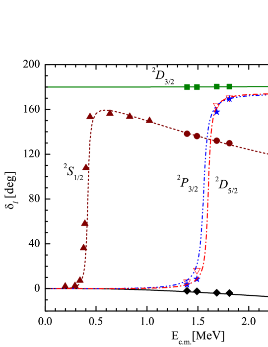
Figure 1: The phase shifts for $p-^{12}$C elastic scattering within the $\textrm{V}_{\textrm{M1}}$ potential model. The experimental data are taken from Refs. dub08 ; brown67 .

The empirical ANC values reported in Table 1 were derived from the analysis of the cross-section of the proton transfer reaction using the modified DWBA art22 ; art02 and the continuum discretized coupled channels (CDCC) method fernan00 . The elastic $p-^{12}$C scattering in low energy region was previously studied within the halo effective field theory in24 and the multilevel, multichannel R-matrix approach azuma10 . As can be seen from Fig. 1, the experimental phase shifts are well described within the proposed potential models.

Table 2: Parameters of the $S$-, $P$- and $D$- wave resonances of the ¹³N nucleus, calculated within different potential models, in comparison with the experimental data

${}^{2S+1}L_{J}$	$E_{x}$	$J_{i}^{\pi}$ (MeV)	$\Gamma_{c.m.}$(exp.) (keV)	$E_{res}$ (exp.) (keV)	$\Gamma_{c.m.}$(theory) (keV)	$E_{res}$ (theory) (keV)
${}^{2}S_{1/2}$ ($\textrm{V}_{\textrm{M1}}$)	2.365	$1/2^{+}$	35.2$\pm$0.5 gyur23b	424.2$\pm$0.7 gyur23b	36	422
${}^{2}S_{1/2}$($\textrm{V}_{\textrm{M2}}$)					35	424
${}^{2}S_{1/2}$ ($\textrm{V}_{\textrm{M3}}$)					35	427
${}^{2}S_{1/2}$($\textrm{V}_{\textrm{M4}}$)					39	424
${}^{2}P_{3/2}$	3.502	$3/2^{-}$	62$\pm$4 ajzen91	1558.5$\pm$2 ajzen91	62	1558
${}^{2}D_{5/2}$	3.547	$5/2^{+}$	45.2$\pm$0.5 kett23	1601.0$\pm$0.5 kett23	44	1603

The $p-^{12}$C system in the $S$-wave contains a Pauli forbidden state according to the classification of orbital states of the Young’s diagrams dub25 . In the last column of Table 1, the energy values of the Pauli forbidden state in the ${}^{2}S_{1/2}$ partial wave are given for the different potential models. Properties of the most important ¹³N$(1/2^{+})$ resonance ($E_{x}$=2.365 MeV) in this partial wave have been studied within the framework of different theoretical approaches in Refs. kett23 ; gyur23b ; dub25 ; ajzen91 ; tur23b and the width of the resonance was estimated to belong to the 30.1 keV $-$ 37.8 keV interval.

The resonance energies $E_{res}$ and widths $\Gamma$ of the ¹³N nucleus in the ${}^{2}P_{3/2}$ and ${}^{2}D_{5/2}$ partial waves are also presented in Table  2. As can be seen from the table, the existing experimental data  kett23 ; gyur23b ; ajzen91 are well described within the developed potential model approach.

III Astrophysical $S$ factor of the ${}^{12}{\rm C}(p,\gamma)^{13}{\rm N}$ direct capture reaction

The contributions of the electromagnetic $E1$, $E2$ and $M1$ transition operators into the astrophysical $S$ factor of the ${}^{12}{\rm C}(p,\gamma)^{13}{\rm N}$ reaction are shown in Figure 2 for the model $\textrm{V}_{\textrm{M${\rm{1}}$}}$ from Table 1. As is known from the literature bur08 and as can be seen in the figure, the two resonant states $1/2^{+}$ ($E_{x}$=2.365 MeV) and $3/2^{-}$ ($E_{x}$=3.502 MeV) yield the most important contribution to the direct radiative capture process through the electric ${}^{2}S_{1/2}\rightarrow^{2}P_{1/2}$ and magnetic ${}^{2}P_{3/2}\rightarrow^{2}P_{1/2}$ dipole transitions to the ${}^{13}{\rm N}$ ground state. The transition from the $1/2^{+}$ resonance state completely dominates in the region below 1 MeV, while the magnetic transition from the ${}^{2}P_{3/2}$ state dominates beyond this region up to the reaction energy of about 2 MeV. This is why the problem of the consistent description of the properties of these resonances is of crucial importance.

As can be seen from Figure 2, the electric ${}^{2}D_{3/2}\rightarrow^{2}P_{1/2}$ dipole transition plays a minor role for the process below 1 MeV. The contributions of the electric quadrupole transition ($E$2) ${}^{2}P_{3/2}\rightarrow^{2}P_{1/2}$ is even more suppressed, while the contribution from magnetic dipole ($M$1) ${}^{2}P_{1/2}\rightarrow^{2}P_{1/2}$ transition operators is entirely negligible in the astrophysical energy region.

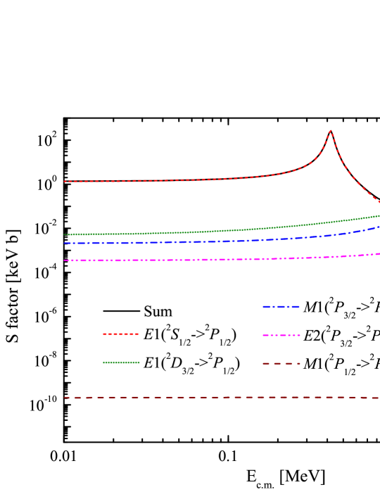
Figure 2: The $E$1, $E$2 and $M1$ partial transition contributions to the astrophysical $S$ factor from different initial scattering states to the final ${}^{13}\rm{N(1/2^{-})}$ ground state within the potential model $\textrm{V}_{\textrm{M1}}$.

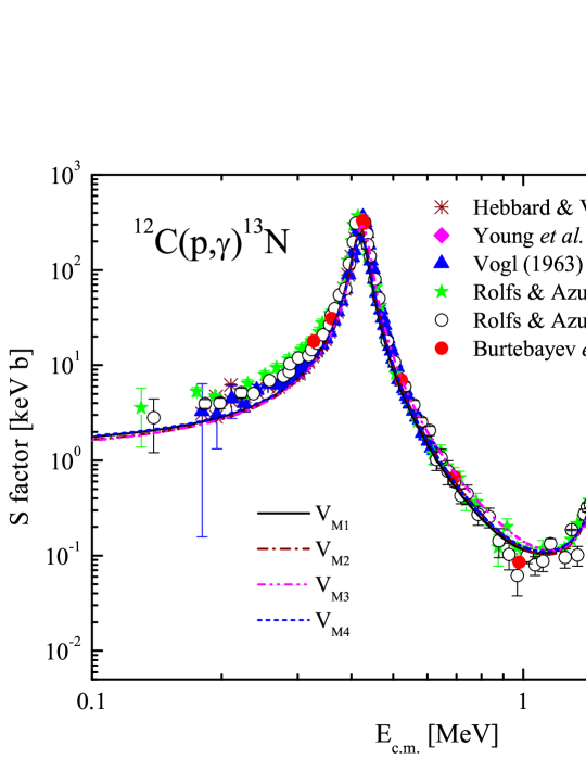
Figure 3: Astrophysical $S$ factor for the ¹²C(p,$\gamma)^{13}$N synthesis reaction, estimated within different potential models in comparison with the experimental data from Refs. heb60 ; young63 ; vogl63 ; rolfs74 ; bur08 .

In Fig. 3 the calculated astrophysical $S$ factors of the direct radiative capture reaction ${}^{12}{\rm C}(p,\gamma)^{13}{\rm N}$ within the potential models $\textrm{V}_{\textrm{M${\rm{1}}$}}$, $\textrm{V}_{\textrm{M${\rm{2}}$}}$, $\textrm{V}_{\textrm{M${\rm{3}}$}}$ and $\textrm{V}_{\textrm{M${\rm{4}}$}}$ are compared with the old experimental data sets from Refs.  heb60 ; young63 ; vogl63 ; rolfs74 ; bur08 . And in Fig. 4, the theoretical results are compared with the most recent experimental data sets of the LUNA Collaboration  luna23 resulting from the direct measurements and other recent data sets from Refs.  skow23 ; gyur23a ; kett23 within the whole astrophysical low-energy region. As can be seen from the figures, the agreement between theoretical results and experimental data sets is very good. Clearly, the theoretical models describe the newest data sets from 2023 more accurately. However, from these figures one can not make a conclusion about the advantages or disadvantages of the above models since they all describe the existing data sets at the same high level.

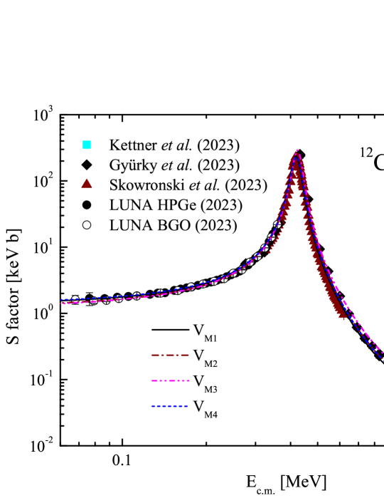
Figure 4: Astrophysical $S$ factor for the ¹²C(p,$\gamma)^{13}$N synthesis reaction, estimated within different potential models in comparison with the newest experimental data from Refs. skow23 ; luna23 ; gyur23a ; kett23 .

It should be noted that the old experimental data points were obtained down to the center-of-mass energy of 130 keV rolfs74 , while the newest experimental points shown in Fig. 4 were determined down to extremely low energy of 68 keV luna23 thanks to the condition in a background-shielded at a depth of 1400 meters. However, the new experimental points skow23 ; gyur23a , which correspond to the energy region around the first resonance ($E_{x}$=2.365 MeV; $1/2^{+}$) peak, are about 40-50 percent lower than the old data vogl63 ; rolfs74 ; bur08 . From this point of view, one can argue that the best description of the new experimental data for the astrophysical $S$ factor of the ¹²C(p,$\gamma)^{13}$N direct capture process corresponds to the $\textrm{V}_{\textrm{M1}}$ and $\textrm{V}_{\textrm{M4}}$ potential models. The latter yield the ANC value of 1.63$\pm$0.13 fm^-1/2 for the ${}^{13}\rm{N(1/2^{-})}$ ground state art22 .

In Table  3 the calculated values of the astrophysical $S(E)$ factor of the direct ¹²C(p,$\gamma)^{13}$N capture process at zero and at the solar Gamow peak $S(25~\rm{keV})$ energy are given for the potential models developed above. The zero-energy astrophysical $S(0)$ factor was estimated by using the asymptotic expansion method baye00 . The method was previously used to calculate $S(0)$ factors for the ³He$(\alpha,\gamma)^{7}$Be, ³H$(\alpha,\gamma)^{7}$Li, and ⁷Be$(p,\gamma)^{8}$B capture reactions resulting estimates consistent with other available data tur23c . The theoretical results obtained within the all four potential models developed in present work, particularly are consistent with the Solar Fusion II result of $S(0)=1.34\pm 0.21$ keV b adel11 .

Table 3: The calculated values of the astrophysical $S(E)$ factor at the zero and solar Gamow energies.

E${}^{\rm{*}}~\rm{(keV)}$	S(E) (keV b)
	$\rm{V}_{\rm{M1}}$	$\rm{V}_{\rm{M2}}$	$\rm{V}_{\rm{M3}}$	$\rm{V}_{\rm{M4}}$
0.0	1.33	1.21	1.17	1.35
25	1.41	1.29	1.25	1.44

On the other hand, the calculated values of the astrophysical $S$ factor at the solar Gamow energy 1.41 keV b and 1.44 keV b within the $\textrm{V}_{\textrm{M${\rm{1}}$}}$ and $\textrm{V}_{\textrm{M${\rm{4}}$}}$ models, respectively, are in good agreement with the result of the R-matrix fit of $S(25~\rm{keV})=1.48\pm 0.09$ keV b by Kettner et al. kett23 , but slightly lower than the result of $S(25~\rm{keV})=1.53\pm 0.06$ keV b by the LUNA Collaboration luna23 ; achar24 . At the same time, the models $\textrm{V}_{\textrm{M${\rm{2}}$}}$ and $\textrm{V}_{\textrm{M${\rm{3}}$}}$ yield somewhat smaller estimates for this value.

IV Reaction rates of the ${}^{12}{\rm C}(p,\gamma)^{13}{\rm N}$ astrophysical direct capture process

For the estimation of chemical element abundances in the stars, one needs to evaluate the values of nuclear reaction rates on the basis of the calculated cross-sections. This quantity cannot be extracted from the data of the experimental measurements. The well-known expression for the reaction rate $N_{A}(\sigma v)$ reads nacre ; fow1975

$$N_{A}(\sigma v)=N_{A}\frac{(8/\pi)^{1/2}}{\mu^{1/2}(k_{\text{B}}T)^{3/2}}\int^{\infty}_{0}\sigma(E)E\exp(-E/k_{\text{B}}T)dE,$$ (8)

where $\sigma(E)$ is the calculated cross-section of the process, $k_{\text{B}}$ is the Boltzmann coefficient, $T$ is the temperature, $N_{A}=6.0221\times 10^{23}\,\text{mol}^{-1}$ is the Avogadro number.

Table 4: The ${}^{12}{\rm C}(p,\gamma)^{13}{\rm N}$ astrophysical reaction rates $N_{A}(\sigma v)$ ($\textrm{cm}^{3}\rm{mol}^{-1}\rm{s}^{-1}$) in the temperature interval $0.001\leq T_{9}\leq 10$ calculated within the $\textrm{V}_{\textrm{M1}}$ and $\textrm{V}_{\textrm{M4}}$ potential models.

$T_{{\rm{9}}}$	$\textrm{V}_{\textrm{M1}}$	$\textrm{V}_{\textrm{M4}}$	$T_{{\rm{9}}}$	$\textrm{V}_{\textrm{M1}}$	$\textrm{V}_{\textrm{M4}}$
0.001	$6.84\times 10^{-51}$	$6.99\times 10^{-51}$	0.14	$3.74\times 10^{-4}$	$3.83\times 10^{-4}$
0.002	$7.98\times 10^{-39}$	$8.16\times 10^{-39}$	0.15	$6.68\times 10^{-4}$	$6.84\times 10^{-4}$
0.003	$5.66\times 10^{-33}$	$5.79\times 10^{-33}$	0.16	$1.14\times 10^{-3}$	$1.17\times 10^{-3}$
0.004	$2.76\times 10^{-29}$	$2.82\times 10^{-29}$	0.18	$2.95\times 10^{-3}$	$3.03\times 10^{-3}$
0.005	$1.16\times 10^{-26}$	$1.18\times 10^{-26}$	0.20	$6.81\times 10^{-3}$	$6.97\times 10^{-3}$
0.006	$1.15\times 10^{-24}$	$1.18\times 10^{-24}$	0.25	$4.01\times 10^{-2}$	$4.09\times 10^{-2}$
0.007	$4.55\times 10^{-23}$	$4.66\times 10^{-23}$	0.30	$1.89\times 10^{-1}$	$1.90\times 10^{-1}$
0.008	$9.42\times 10^{-22}$	$9.65\times 10^{-22}$	0.35	$7.60\times 10^{-1}$	$7.57\times 10^{-1}$
0.009	$1.22\times 10^{-20}$	$1.25\times 10^{-20}$	0.40	$2.50\times 10^{0}$	$2.48\times 10^{0}$
0.010	$1.11\times 10^{-19}$	$1.13\times 10^{-19}$	0.45	$6.74\times 10^{0}$	$6.66\times 10^{01}$
0.011	$7.60\times 10^{-19}$	$7.78\times 10^{-19}$	0.5	$1.52\times 10^{1}$	$1.51\times 10^{1}$
0.012	$4.18\times 10^{-18}$	$4.28\times 10^{-18}$	0.6	$5.25\times 10^{1}$	$5.19\times 10^{1}$
0.013	$1.92\times 10^{-17}$	$1.96\times 10^{-17}$	0.7	$1.26\times 10^{2}$	$1.25\times 10^{2}$
0.014	$7.59\times 10^{-17}$	$7.77\times 10^{-17}$	0.8	$2.39\times 10^{2}$	$2.38\times 10^{2}$
0.015	$2.64\times 10^{-16}$	$2.71\times 10^{-16}$	0.9	$3.88\times 10^{2}$	$3.87\times 10^{2}$
0.016	$8.28\times 10^{-16}$	$8.48\times 10^{-16}$	1	$5.64\times 10^{2}$	$5.63\times 10^{2}$
0.018	$6.24\times 10^{-15}$	$6.39\times 10^{-15}$	1.25	$1.06\times 10^{3}$	$1.06\times 10^{3}$
0.020	$3.55\times 10^{-14}$	$3.63\times 10^{-14}$	1.5	$1.55\times 10^{3}$	$1.56\times 10^{3}$
0.025	$1.15\times 10^{-12}$	$1.18\times 10^{-12}$	1.75	$1.96\times 10^{3}$	$1.98\times 10^{3}$
0.030	$1.64\times 10^{-11}$	$1.68\times 10^{-11}$	2	$2.29\times 10^{3}$	$2.32\times 10^{3}$
0.040	$7.79\times 10^{-10}$	$7.98\times 10^{-10}$	2.5	$2.72\times 10^{3}$	$2.76\times 10^{3}$
0.050	$1.21\times 10^{-8}$	$1.24\times 10^{-8}$	3	$2.95\times 10^{3}$	$3.00\times 10^{3}$
0.060	$9.86\times 10^{-8}$	$1.01\times 10^{-7}$	3.5	$3.05\times 10^{3}$	$3.11\times 10^{3}$
0.070	$5.25\times 10^{-7}$	$5.38\times 10^{-7}$	4	$3.10\times 10^{3}$	$3.15\times 10^{3}$
0.080	$2.09\times 10^{-6}$	$2.14\times 10^{-6}$	5	$3.11\times 10^{3}$	$3.16\times 10^{3}$
0.090	$6.73\times 10^{-6}$	$6.90\times 10^{-6}$	6	$3.09\times 10^{3}$	$3.14\times 10^{3}$
0.10	$1.85\times 10^{-5}$	$1.89\times 10^{-5}$	7	$3.08\times 10^{3}$	$3.13\times 10^{3}$
0.11	$4.47\times 10^{-5}$	$4.58\times 10^{-5}$	8	$3.09\times 10^{3}$	$3.14\times 10^{3}$
0.12	$9.79\times 10^{-5}$	$1.00\times 10^{-4}$	9	$3.14\times 10^{3}$	$3.18\times 10^{3}$
0.13	$1.98\times 10^{-4}$	$2.03\times 10^{-4}$	10	$3.22\times 10^{3}$	$3.26\times 10^{3}$

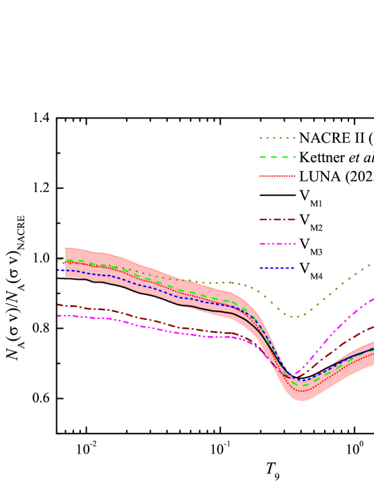
Figure 5: The ¹²C(p,$\gamma)^{13}$N astrophysical reaction rates, normalized to the NACRE rate nacre , estimated within different potential models, in comparison with the results of Refs. nacre2 ; kett23 ; luna23 .

In Fig. 5 the calculated reaction rates within the potential models $\textrm{V}_{\textrm{M${\rm{1}}$}}$, $\textrm{V}_{\textrm{M${\rm{2}}$}}$, $\textrm{V}_{\textrm{M${\rm{3}}$}}$ and $\textrm{V}_{\textrm{M${\rm{4}}$}}$, normalized to the NACRE rate nacre , are compared with the empirical results of Refs. nacre2 ; kett23 ; luna23 in the temperature range from $T_{9}$=0.006 to $T_{9}$=10, where $T_{9}$ is the temperature in the 10⁹ K unit. The shaded area represents the uncertainty of the empirical results of the LUNA Collaboration luna23 . As can be seen in the figure, the models $\textrm{V}_{\textrm{M${\rm{1}}$}}$ and $\textrm{V}_{\textrm{M${\rm{4}}$}}$ yield results, very consistent with the results of the LUNA collaboration luna23 and those from the R-matrix fit kett23 . They reproduce the both absolute values and temperature dependence of the empirical results. At the same time, the models $\textrm{V}_{\textrm{M${\rm{2}}$}}$ and $\textrm{V}_{\textrm{M${\rm{3}}$}}$ do not give satisfactory results. They underestimate the empirical results in the temperature interval below the minimum point at $T_{9}$=0.4 ($T=4\times 10^{-8}$ K) and overestimate them in the temperature region above this point.

As we can remember from Table 1, the models $\textrm{V}_{\textrm{M${\rm{1}}$}}$ and $\textrm{V}_{\textrm{M${\rm{4}}$}}$ yield the ANC value 1.63 fm^-1/2 of the virtual decay ¹³ N(1/2^-)$\to^{12}$C$+p$, which turns out to be the most realistic. We also recall that these models differ from each other only in the description of the width of the $S$- wave $1/2^{+}$ resonance at the excitation energy $E_{x}=2.365$ MeV. One can see from Fig. 5, that the results most close to the LUNA line belong to the model $\textrm{V}_{\textrm{M${\rm{4}}$}}$, which yields the $1/2^{+}$ resonance width of 39 keV, while the model $\textrm{V}_{\textrm{M${\rm{1}}$}}$ gives 36 keV. This means that the reaction rates of the ¹²C$(p,\gamma)^{13}$N direct capture process is extremely sensitive to the description of the $1/2^{+}$ resonance at $E_{x}=2.365$ MeV. The recommended theoretical value for the width is slightly larger than the experimental widths of $\Gamma=35.2\pm 0.5$ keV gyur23b and $\Gamma=36.0\pm 1.9$ keV rolfs74 . One can expect that this problem can be clarified in further theoretical and experimental research studies.

V Conclusion

The potential model was developed to study the astrophysical direct nuclear capture process ¹²C($p,\gamma)^{13}$N. The Woods-Saxon form of the phase-equivalent potentials for the $p-^{12}$C interaction have been examined for their ability to describe the experimental data on the astrophysical $S$ factor and the reaction rates of the process. The parameters of the $p-^{12}$C potentials are fitted to reproduce the bound state properties (binding energy and the ANC), as well as the experimental phase shifts in the scattering channels.

It was shown found, that the reaction rates of the process are very sensitive to the description of the ANC of the ¹³N(1/2^-) ground state and $S$- wave N($1/2^{+}$) resonance width at the excitation energy $E_{x}=2.365$ MeV. The potential model which reproduce the empirical value of ANC, $C=1.63$ fm^-1/2 and the width $\Gamma=39$ keV of the N$(1/2^{+})$ resonance, yields a very good description of the new experimental data for the astrophysical $S$ factor and the empirical reaction rates of the LUNA Collaboration. The calculated values of the astrophysical $S$ factor at the solar Gamow energy are in good agreement with the result of $S(25~\rm{keV})=1.48\pm 0.09$ keV b obtained by Kettner et al. kett23 using the R-matrix fit, but slightly lower than the result of the LUNA Collaboration luna23 ; achar24 of $S(25~\rm{keV})=1.53\pm 0.06$ keV b.

References

- (1) C. Iliadis, Nuclear Physics of Stars, 2nd ed. (Wiley-VCH, Weinheim, Germany, 2015).
- (2) Borexino Collaboration (M. Agostini, et al.), Nature 587, 577 (2020).
- (3) D. Clayton, Handbook of Isotopes in the Cosmos: Hydrogen to Gallium, (Cambrige University Press, 2003).
- (4) B. Acharya, M. Aliotta, A.B. Balantekin, et al., arXiv: 2405.06470, (2024).
- (5) J. Skowronski, E. Masha, D. Piatti, M. Aliotta, H. Babu, D. Bemmerer et al., Phys. Rev. C 107, L062801 (2023).
- (6) LUNA Collaboration (J. Skowronski, et al.), Phys. Rev. Lett. 131, 162701 (2023).
- (7) LUNA Collaboration (J. Skowronski, et al.), Phys. Rev. C 111, 035802 (2025).
- (8) Gy. Gyürky, L. Csedreki, T. Szücs, G.G. Kiss, Z. Halász, and Zs. Fülöp, Eur. Phys. Jour. A 59, 59 (2023).
- (9) L. Csedreki, Gy. Gyürky, and T. Szücs, Nucl. Phys. A 1037, 122705 (2023).
- (10) K-U. Kettner, H.W. Becker, C.R. Brune, R.J. deBoer, J. Görres, D. Odell, D. Rogalla, and M. Wiescher, Phys. Rev. C 108, 035805 (2023).
- (11) C. Cockcroft, C. Gilbert, and E. Walton, Nature (London) 133, 328 (1934).
- (12) L. Hafstad and M.A. Tuve, Phys. Rev. 48, 306 (1935).
- (13) C.L. Bailey and W.R. Stratton, Phys. Rev. 77, 194 (1950).
- (14) R.N. Hall and W.A. Fowler, Phys. Rev. 77, 197 (1950).
- (15) D.F. Hebbard and J.L. Vogl, Nucl. Phys. 21, 652 (1960).
- (16) J.L. Vogl, PhD thesis, California Institute of Technology, Pasadena, California, 1963.
- (17) F.C. Young, J.C. Armstrong, and J.B. Marion, Nucl. Phys. 44, 486 (1963).
- (18) C. Rolfs and R.E. Azuma, Nucl. Phys. A 227, 291 (1974).
- (19) N.A. Burtebayev, S.B. Igamov, R.J. Peterson, R. Yarmukhamedov, and D.M. Zazulin, Phys. Rev. C 78, 035802 (2008).
- (20) R.E. Azuma, E. Uberseder, E.C. Simpson, C.R. Brune, H. Costantini, R.J. de Boer, J. Görres, M. Heil, P.J. LeBlanc, C. Ugalde, and M. Wiescher, Phys. Rev. C 81, 045805 (2010).
- (21) M. Wiescher, R.J. deBoer, and J. Görres, Frontiers in Physics 10, 1009489 (2022).
- (22) J.T. Huang, C.A. Bertulani, and V. Guimarães, At. Data Nucl. Data Tables 96, 824 (2010).
- (23) B.F. Irgaziev, J-U. Nabi, and A. Kabir, Astrophys Space Sci. 363, 148 (2018).
- (24) A. Kabir, B.F. Irgaziev, and J-U. Nabi, Braz. Jour. Phys. 50, 112 (2020).
- (25) S.B. Dubovichenko, N.A. Burkova, A.S. Tkachenko, and A. Samratova, Chin.Phys.Jour. 49, 044104 (2025).
- (26) M. Dufour and P. Descouvemont, Phys. Rev. C 56, 1831 (1997).
- (27) M.M. Khansari, H. Khalili, and H. Sadeghi, New Astronomy 57, 76 (2017).
- (28) Z.H. Li, J. Su, B. Guo, E.T. Li, Z.C. Li, et al., Nucl. Phys. A 834, 661 (2010).
- (29) S.V. Artemov, R. Yarmukhamedov, N.A. Burtebayev et al., Eur. Phys. Jour. A 58, 24 (2022).
- (30) S.V. Artemov, E.A. Zaparov, G.K. Nie, M. Nadirbekov, and R. Yarmukhamedov, Izv. RAN (Bull. Russ. Acad. Sci.) Ser. Fiz. 66, 60 (2002).
- (31) J.C. Fernandes, R. Crespo, and F.M. Nunes, Phys. Rev. C 61, 064616 (2000).
- (32) N.K. Timofeyuk, Phys. Rev. C 88, 044315 (2013).
- (33) A.M. Mukhamedzhanov and L.D. Blokhintsev, Eur. Phys. J. A 58, 29 (2022).
- (34) E.M. Tursunov, S.A. Turakulov, and A.S. Kadyrov, Nucl.Phys. A 1006, 122108 (2021).
- (35) E.M. Tursunov, S.A. Turakulov, A.S. Kadyrov, and L.D. Blokhintsev, Phys. Rev. C 104, 045806 (2021).
- (36) E.M. Tursunov, S.A. Turakulov, and K.I. Tursunmakhatov, Phys. Rev. C 108, 065801 (2023).
- (37) E.M. Tursunov and S.A. Turakulov, Nucl.Phys. A 1051, 122931 (2024).
- (38) W. Trächslin and L. Brown, Nucl. Phys. A 101, 273 (1967).
- (39) S.B. Dubovichenko, Russ. Phys. Jour. 51, 1136 (2008).
- (40) E.J. In, T-S. Park, Y-H. Song, and S-W. Hong, Phys. Rev. C 109, 054622 (2024).
- (41) F. Ajzenberg-Selove, Nucl. Phys. A 523, 1 (1991).
- (42) S.A. Turakulov, S.V. Artemov, and R. Yarmukhamedov, Russ. Phys. Jour. 65, 2086 (2023).
- (43) D. Baye and E. Brainis, Phys. Rev. C 61, 025801 (2000).
- (44) S.A. Turakulov and E.M. Tursunov, Acta Phys. Pol. B Proc. Suppl. 16, 2-A3 (2023).
- (45) E.G. Adelberger et al., Rev. Mod. Phys. 83, 195 (2011).
- (46) NACRE (C. Angulo, M. Arnould, M. Rayet, P. Descouvemont, D. Baye, C. Leclercq-Willain, A. Coc, S. Barhoumi, P. Aguer, C. Rolfs et al.), Nucl. Phys. A 656, 3 (1999).
- (47) W.A. Fowler, G.R. Gaughlan, and B.A. Zimmerman, Ann. Rev. Astron. Astrophys. 13, 69 (1975).
- (48) NACRE II (Y. Xu, K. Takahashi, S. Goriely, M. Arnould, M. Ohta, and H. Utsunomiya), Nucl. Phys. A 918, 61 (2013).