Selftok: Discrete Visual Tokens of Autoregression, by Diffusion, and for Reasoning

Abstract

We completely discard the conventional spatial prior in image representation and introduce a novel discrete visual tokenizer: Self-consistency Tokenizer (Selftok). At its design core, we compose an autoregressive (AR) prior—mirroring the causal structure of language—into visual tokens by using the reverse diffusion process of image generation. The AR property makes Selftok fundamentally distinct from traditional spatial tokens in the following two key ways:

$\bullet$ Selftok offers an elegant and minimalist approach to unify diffusion and AR for vision-language models (VLMs): By representing images with Selftok tokens, we can train a VLM using a purely discrete autoregressive architecture—like that in LLMs—without requiring additional modules or training objectives.
$\bullet$ We theoretically show that the AR prior satisfies the Bellman equation, whereas the spatial prior does not. Therefore, Selftok supports reinforcement learning (RL) for visual generation with effectiveness comparable to that achieved in LLMs.

Besides the AR property, Selftok is also a SoTA tokenizer that achieves a favorable trade-off between high-quality reconstruction and compression rate. We use Selftok to build a pure AR VLM for both visual comprehension and generation tasks. Impressively, without using any text-image training pairs, a simple policy gradient RL working in the visual tokens can significantly boost the visual generation benchmark, surpassing all the existing models by a large margin. Therefore, we believe that Selftok effectively addresses the long-standing challenge that visual tokens cannot support effective RL. When combined with the well-established strengths of RL in LLMs, this brings us one step closer to realizing a truly multimodal LLM. Project Page: https://selftok-team.github.io/report/.

1 Introduction

There is a growing consensus that language data will soon be exhausted by large language models (LLMs), whereas non-language data like images or videos are significantly underutilized [105]. Therefore, unifying multiple modalities is a key step toward unlocking AI’s more powerful emergent capabilities. To unify all modalities into one discrete autoregressive model (dAR) like LLMs, we need to tokenize non-language modalities into discrete tokens. In this paper, we only discuss visual discrete tokens and use them together with language to train a vision-language model (VLM) that can do both visual comprehension (i.e., language output like VQA) and generation (i.e., visual output like image synthesis).

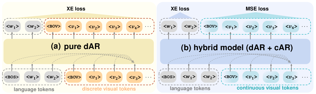
Figure 1: Comparison of (a) pure discrete autoregressive model (dAR) and (b) hybrid model that combines dAR and continuous autoregressive model (cAR). <BOS>/<BOV> indicates the start of a sentence/image. <$w_{i}$>/<$v_{i}$> denotes the $i$-th language/visual token. Both models predict the next token given all previous ones, e.g., [<BOS>, …, <$v_{3}$>] $\to$<$v_{4}$>.

1.1 Why Discrete?

Before introducing our Selftok visual tokenizer, we need to clarify why we advocate the use of a pure dAR (Figure 1), rather than a hybrid approach that combines a dAR for language and a continuous autoregressive model (cAR) for images (Figure 1) [133, 62]. The latter is widely adopted by proponents who argue that visual data should be encoded as continuous tokens to minimize the compression loss, but this is just a minor concern—there are many post-processing methods available to ensure the precision [23, 77, 107, 63]. However, using cAR (or hybrid) leads to major issues that cannot be fundamentally resolved without adopting a pure dAR:

• cAR cannot inherit the successful infrastructure and training paradigm of LLMs. This is the most common reason cited in existing dAR-based VLMs [108, 116, 1, 13, 56]. Yet, the following three justifications are often overlooked by the community.

• cAR is more error-prone in next-token prediction. While dAR functions as a sequential token classifier trained with cross-entropy (XE) loss, cAR operates as a sequential vector regressor trained with mean squared error (MSE) loss, which is less stable and harder to optimize than XE [46, 12]. Perhaps this is the key reason why most cARs abandon the causal next-token prediction and revert to bidirectional modeling, such as demasking [62, 127] or holistic reconstruction [133, 73]. Unfortunately, they undermine the core design philosophy of the decoder-only AR: the causal dependency of tokens [91].

• cAR introduces unnecessary complexity into reinforcement learning (RL). It is widely known that RL is an indispensable post-training step to unleash the power of LLMs [36]. However, cAR turns the finite Markov Decision Process (MDP) formulation of dAR—with a discrete state-action space—into an infinite MDP with a continuous state-action space, thereby complicating policy optimization [75].

• Continuous representations are less disentangled than discrete ones. Disentanglement uncovers the modular and true generative factors of data [42, 115], which are critical for: 1) Unbiased visual comprehension, e.g., if “color” and “object” are disentangled, the model can still recognize a black swan as swan, even if all the training examples of swans are white; and 2) Controlled generation, if such disentanglement holds, the model can generate a black swan without seeing one in training. Since a real-valued vector is infinitely countable, a single continuous token may theoretically entangle all the factor combinations. As a result, achieving disentanglement would require an impractically large amount of training data to cover all the combinations [69], e.g., we need $\mathcal{O}(N^{M})$ images, where $N$ is #values per factor and $M$ is the #factors per image. In contrast, discrete tokens, with their limited information bandwidth, serve as a strong inductive bias that encourages disentanglement [44].

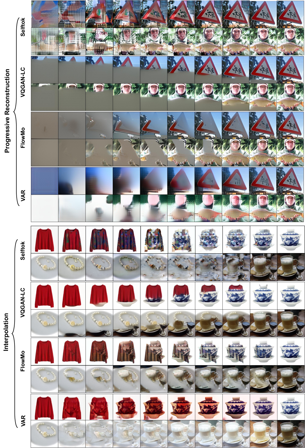
Figure 2: Progressive reconstruction (left to right): Reconstructions by progressively masking out a shorter sequence of tokens before inputting to the decoder. Interpolation (left to right): Reconstructions by gradually replacing tokens of the left image with those of the right one. All methods except Selftok exhibit strong spatial characteristics (i.e., tokens$\Leftrightarrow$patches).

1.2 Why Not Spatial?

Since representing an image as a set of spatial grids has been the standard approach back in the early days of computer vision, it is often assumed—almost by default—that spatial tokens are naturally suited for AR modeling like language. However, we overlook the fact that the causal dependencies among spatial tokens are inherently not autoregressive and thus cannot be modeled in the same way as language using AR models.

First, as shown in Figure 3, since spatial pixels (the cause) collectively form the image (the effect), observing any part of the image during spatial token encoding can introduce spurious dependencies among the tokens due to the collider effect [86], i.e., the resulting Bayesian causal graph of spatial tokens is not as autoregressive as that of AR tokens (Figure 5).

Second, we reveal a significant drawback of spatial tokens that has previously gone unnoticed: non-AR dependency fundamentally violates the policy improvement optimality in RL [106]. To illustrate this in Figure 3, in non-AR dependency, token prediction (action) at a later time affects the tokens predicted in earlier steps (earlier states), so the later policy may contradict earlier policies that have already been optimized. Compared to AR tokens, RL for non-AR spatial tokens is expected to be significantly less effective (Section 4.3).

Based on the above two reasons, we conjecture that the misuse of spatial tokens—whether discrete or continuous— is the key reason why AR-based VLMs do not scale as effectively as LLMs. We leave the large-scale empirical validation of this hypothesis to future work.

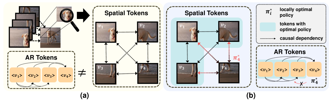
Figure 3: (a) As an image can be viewed as the effect of spatial pixels (or patches), observing any part of it introduces spurious dependencies among spatial tokens, making them non-AR. (b) Due to the anti-causal links (red) for spatial tokens, learning the locally optimal policy $\pi^{*}_{4}$ for a later token (e.g., $v_{4}$) can propagate backward and interfere with earlier tokens that were already optimized (e.g., $v_{1},v_{2},v_{3}$). In contrast, AR tokens without such links do not have this issue. A more formal illustration is in Section 4.1.

1.3 Contributions

We propose Selftok: Self-consistency Tokenizer, which encodes an image into autoregressive discrete tokens, where each token corresponds to a diffusion time step. Therefore, Selftok can be integrated into a single dAR-based VLM, which can reason like LLMs but in the visual domain. The following summarizes our contributions and provides a reading guide to the rest of the paper.

1) Selftok of Autoregression: Compared to conventional spatial tokens, Selftok completely abandons the long-standing spatial prior without compromising reconstruction quality (Section 2.3) and spatial understanding (Section 3.2). More importantly, thanks to the AR property, Selftok offers better language compatibility of images, leading to improved dAR-based VLM training (Section 3) and effective RL-based post-training (Section 4).

2) Selftok by Diffusion: Selftok leverages the AR nature of the reverse diffusion process and encodes the entire trajectory of image generation (Figure 2&Section 2.1). Therefore, it offers one of the most elegant yet straightforward approaches to unify diffusion and AR into a single dAR framework, in contrast to existing methods that rely on additional architectures or training objectives incompatible with dAR.

3) Selftok for Reasoning: Thanks to its AR property, Selftok produces visual tokens that satisfy the optimality condition of the policy improvement (Section 4). As a result, Selftok-based VLMs support effective RL-based post-training for visual generation, akin to LLMs, whereas spatial token-based counterparts do not. For example, without using any pairwise supervision, our Selftok-Zero achieves impressive image generation performances on GenEval: 92% (Table 7) and DPG-Bench: 85.57 (Table 8).

The preliminary core ideas of Selftok are presented in [129, 83, 65]. We encourage readers to begin with them before turning to this extended version, which offers a more theoretical analysis and presents more comprehensive and improved results.

2 Selftok: Self-consistency Tokenizer

We begin by unpacking the meaning behind the name Self-consistency. “Self” is just a rephrasing of the concept behind auto-encoder: both the encoder and decoder are trained to reconstruct the input image itself.

Specifically, our goal is to encode an image $I$ into $K$ discrete tokens, i.e., $\mathrm{Enc}(I)=\mathcal{V}_{K}=[v_{1},v_{2},...,v_{K}]$, which can be decoded to reconstruct $I$ while adhering to an autoregressive (AR) prior. We formulate the following constrained optimization:

$$\mathop{\mathrm{min}}_{\mathrm{Enc}(I)=\mathcal{V}_{K},\leavevmode\nobreak\ \mathrm{Dec}}\leavevmode\nobreak\ \|I-\mathrm{Dec}\left(\mathcal{V}_{K}\right)\|^{2},$$ (1)

$$s.t.\;\;P(\mathcal{V}_{K})\overset{\text{AR}}{=}P (v_{1})\cdot P(v_{2}|v_{1})\cdot\ldots\cdot P(v_{K}|v_{1},\ldots,v_{K-1}),$$

where we define $\overset{\text{AR}}{=}$ as a special equality to indicate that the tokens $\mathcal{V}_{K}$ conform to the AR causal graph in Figure 4, i.e., each token is generated from its predecessors. This definition is necessary, as the factorization is always valid for any token sequence through the chain rule of probability and does not necessarily imply an AR structure per se.

As with other discrete compression problems [125], solving the constrained optimization in Eq. (1) is inherently NP-hard due to the combinatorial nature of token assignment. To make this tractable, we introduce an inductive bias grounded in the reverse diffusion process, which jointly satisfies the AR constraint and the reconstruction objective. In particular, the term “Consistency” comes from Consistency Model [102]. Similarly, we use a diffusion model and make the decoder consistent with the image generation path, i.e., reconstructing $\mathbf{x}_{1}=I$ from any noisy inputs $\mathbf{x}_{t}$ along the path.

Next, in Section 2.1, we show how the reverse diffusion process can be formulated in a recursive fashion that enables efficient learning of AR tokens. Then, we present implementation details in Section 2.2 and validation results in Section 2.3.

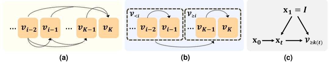
Figure 4: (a) The causal graph for AR, where each dotted direct edge represents a causation. (b) The recursion of the AR causal graph. (c) The causal graph for learning $\mathcal{V}_{\geqslant k(t)}$ in Eq. (5).

2.1 Autoregression and Recursion by Diffusion

We show in Figure 4 that AR structure has an equivalent recursion, enabling a divide-and-conquer approach that decomposes the challenging constraint in Eq. (1) into simpler ones:

$$P(\mathcal{V}_{K})\overset{\text{AR}}{=}P(\mathcal{V}_{<i})\cdot P(\mathcal{V}_{\geqslant i}|\mathcal{V}_{<i}),$$ (2)

where $\mathcal{V}_{<i}=[v_{1},v_{2},...,v_{i-1}]$ and $\mathcal{V}_{\geqslant i}=[v_{i},v_{i+1},...,v_{K}]$. For example, we can recursively apply Eq. (2) until it becomes a trivial learning problem $P(\mathcal{V}_{<K})\cdot P(v_{K}|\mathcal{V}_{<K})$: if $\mathcal{V}_{<K}$ is provided, it is easy to encode the last token $v_{K}$. Interestingly, the reverse diffusion process (in ODE form) has a similar decomposition [68, 103]:

$$\frac{d\mathbf{x}_{t}}{dt}=\mathbf{v}_{t}(\mathbf{x}_{t}),\leavevmode\nobreak\ \leavevmode\nobreak\ t\in[0,1]\;\;\;\;\overset{\text{solution}}{\Longrightarrow}\;\;\;\;\;\;\underbrace{\mathbf{x}_{1}}_{\text{destination}}=\underbrace{\mathbf{x}_{t}}_{\text{midway point }}+\;\;\underbrace{\int_{t}^{1}\mathbf{v}_{s}(\mathbf{x}_{s})ds}_{\begin{subarray}{c}\textrm{path from midway }\\ \textrm{to destination:}\leavevmode\nobreak\ \mathbf{x}_{t}\rightsquigarrow\mathbf{x}_{1}\end{subarray}},$$ (3)

where $\mathbf{v}_{t}(\mathbf{x}_{t})$ is the velocity field at time-step $t$ that transports the noisy midway $\mathbf{x}_{t}$, starting from $\mathbf{x}_{0}\in\mathcal{N}(0,1)$, towards the clean image $\mathbf{x}_{1}=I$. This shows that, if the midway $\mathbf{x}_{t}$ is provided, the reconstruction of $\mathbf{x}_{1}$ starting from $\mathbf{x}_{t}$ is easier than directly moving from $x_{0}$ to $x_{1}$.

Hence, we can establish a correspondence between the two recursions by aligning the provided midway point (part 1) and what comes after it (part 2), respectively:

$$\left(\underbrace{P(\mathcal{V}_{K})\Longleftrightarrow\mathbf{x}_{1}}_{\text{Whole}}\right)=\left(\underbrace{P(\mathcal{V}_{<i})\Longleftrightarrow\mathbf{x}_{t}}_{\text{Part 1}}\right)\;\;+\;\;\left(\underbrace{P(\mathcal{V}_{\geqslant i}|\mathcal{V}_{<i})\Longleftrightarrow\int_{t}^{1}\mathbf{v}_{s}(\mathbf{x}_{s})ds}_{\text{Part 2}}\right).$$ (4)

Motivated by this, we aim to compose the AR constraint into the reconstruction in Eq. (1). Specifically, we decompose the entire reconstruction (from pure noise $\mathbf{x}_{0}$ to $\mathbf{x}_{1}$) into two parts with a similar recursion: Part 1: A given $\mathbf{x}_{t}$, sampled from the diffusion path $q(\mathbf{x}_{t}|\mathbf{x}_{1})$, encapsulates $\mathcal{V}_{<i}$, which is assumed to be already encoded; and Part 2: The reconstruction from $\mathbf{x}_{t}$ to $\mathbf{x}_{1}$ for learning the tokens $\mathcal{V}_{\geqslant i}=[v_{i},v_{i+1},\ldots,v_{K}]$. Now, we present the Selftok training objective for an image sample $\mathbf{x}_{1}=I$:

$$\text{Selftok objective}:\mathop{\mathrm{min}}_{\begin{subarray}{c}\mathrm{Enc}(\mathbf{x}_{1})=\mathcal{V}_{K},\\ \mathrm{Dec}\end{subarray}}\leavevmode\nobreak\ \leavevmode\nobreak\ \mathop{\mathbb{E}}_{t\in[0,1]}\;\left[\mathop{\mathbb{E}}_{\mathbf{x}_{t}\sim q(\mathbf{x}_{t}|\mathbf{x}_{1})}\left[\|\mathbf{x}_{1}-\mathrm{Dec}(\mathbf{x}_{t},\mathcal{V}_{\geqslant k(t)})\|^{2}\right]\right],$$ (5)

where $\mathcal{V}_{\geqslant k(t)}=[v_{k(t)},v_{k(t)+1},...,v_{K}]$ and $k(t)$ is a token schedule with $k(1)=K+1$ and $k(0)=1$, which maps each continuous time-step $t$ to a discrete token index $i$ in Eq. (4). The choices of $q(\mathbf{x}_{t}|\mathbf{x}_{1})$ and $k(t)$ are discussed in Section 2.2.3&2.2.4, respectively. When the context is clear, we use $k(t)$ and $i$ interchangeably. We highlight that our Sefltok is indeed non-spatial: $\mathcal{V}_{K}$ discretizes the continuous velocity field of the entire image generation path, which is beyond the naïve spatial visual cues. Please recall Figure 2 for qualitative illustrations.

Here, we verify that the Seltok objective in Eq. (5) optimizes the original one in Eq. (1) from the following three aspects:
1) Reconstruction: When $t=0$, Eq. (5) already includes the reconstruction objective in Eq. (1) by considering $\|I-\mathrm{Dec}\left(\mathcal{V}_{K}\right)\|^{2}=\|\mathbf{x}_{1}-\mathrm{Dec}(\mathbf{x}_{0},\mathcal{V}_{K}=\mathcal{V}_{\geqslant k(0)=1})\|^{2}$, because the latter decoder only takes in a new non-informative input: the white noise $\mathbf{x}_{0}$.
2) AR Constraint by Recursive Design: Due to the correspondence between AR and diffusion recursion in Eq. (4), Eq. (5) is a recursive breakdown of Eq. (1) by time-step $t$: $\mathcal{V}_{\geqslant i}$ is learned from the reconstruction $\|\mathbf{x}_{1}-\mathrm{Dec}(\mathbf{x}_{t},\mathcal{V}_{\geqslant k(t)})\|^{2}$ that completes the path $\mathbf{x}_{t}\rightsquigarrow\mathbf{x}_{1}$; whereas the midway point $\mathbf{x}_{t}$ encapsulates $\mathcal{V}_{<i}$, which is considered to be already identified by $\mathbf{x}_{0}\rightsquigarrow\mathbf{x}_{t}$. This satisfies the probability factorization in Eq. (2) and the causal structure in Figure 4.
3) AR Constraint by Causal Identification: To ensure that the learned $\mathcal{V}_{K}$ is indeed of AR structure, i.e., the encoder identifies the causal effect from $\mathcal{V}_{<i}$ to $\mathcal{V}_{\geqslant i}$, we need to justify that Eq. (5) is an unbiased estimate of $\mathcal{V}_{\geqslant i}$ from $\mathbf{x}_{t}$ (i.e., $\mathcal{V}_{<i}$) for all $t\in[0,1]$. To this end, we show that Eq. (5) induces the causal graph in Figure 4: Causation $\mathbf{x}_{0}\to\mathbf{x}_{t}\leftarrow\mathbf{x}_{1}$ denotes that $\mathbf{x}_{t}$ is sampled from $q(\mathbf{x}_{t}|\mathbf{x}_{1})$ by mixing noise $\mathbf{x}_{0}$ and image $\mathbf{x}_{1}$; causation $\mathbf{x}_{t}\to\mathcal{V}_{\geqslant k(t)}\leftarrow\mathbf{x}_{1}$ denotes that the tokens $\mathcal{V}_{\geqslant k(t)}$ are learned from $\mathbf{x}_{1}$ and $\mathbf{x}_{t}$. In this way, $\mathbf{x}_{0}$ serves as an instrument variable (IV) [86], independent of the confounder $\mathbf{x}_{1}$. Recall the re-parametrization: $\mathbf{x}_{t}=\sigma(t)\cdot\mathbf{x}_{0}+\mu(t)\cdot\mathbf{x}_{1}$, where $\sigma(t)$ and $\mu(t)$ can be considered as time-specific constants [68]. Thus, the inner expectation of Eq. (5) can be rewritten as:

$$\mathop{\mathbb{E}}_{\mathbf{x}_{0}\sim\mathcal{N}(0,1)}\left[\|\mathbf{x}_{1}-\mathrm{Dec}\left(\sigma(t)\cdot\mathbf{x}_{0}+\mu(t)\cdot\mathbf{x}_{1},\mathcal{V}_{\geqslant k(t)}\right)\|^{2}\right],$$ (6)

which implies that $\mathcal{V}_{\geqslant k(t)}$ can be directly estimated from the IV $\mathbf{x}_{0}$, ensuring that $\mathcal{V}_{\geqslant k(t)}$ learned from $\mathbf{x}_{t}$ is unbiased, even in the presence of the confounder $\mathbf{x}_{1}$.

Now, we empirically verify that the structure of Selftok is AR by plotting the token prediction entropy curves w.r.t. token positions under three generation orders using a dAR model (Llama 3.1). Besides the normal sequential order $[v_{1},v_{2},v_{3},...]$, we use another two orders: 1) stride-one shuffle, which is a concatenation of subsequence $[v_{1},v_{3},...]$ followed by subsequence $[v_{2},v_{4},v_{6},...]$, and 2) stride-two shuffle, which is a concatenation of subsequence $[v_{1},v_{4},v_{7},...]$, $[v_{2},v_{5},v_{8},...]$, and $[v_{3},v_{6},v_{9},...]$. The design principle of these orders is simple: an ordered subsequence of an AR sequence is still AR. As entropy measures the uncertainty in token prediction, if the sequence is AR, the entropy trend is generally decreasing. Therefore, if the token sequence is AR, the two shuffled orders should demonstrate a segmented decreasing curve. As shown in Figure 5, we can see that only Selftok demonstrates such a segmented decreasing trend corresponding to the three sequence orders.

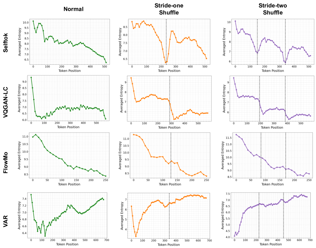
Figure 5: Plots of the next-token prediction entropy versus token position for our Selftok, 2D spatial tokens (VQGAN-LC [134]), 1D tokens (FlowMo [93]), multi-scale 2D tokens (VAR [109]), using the original or shuffled sequences. Only Selftok exhibits a segmented decreasing trend that aligns with the three sequence orders. Although VQGAN-LC also displays a segmented trend, each segment is not decreasing. Conversely, while FlowMo shows a decreasing trend, it is not segmented under the shuffled orders.

2.2 Implementation

Building on the design principles of Selftok outlined above, we now describe the implementation details illustrated in Figure 6&9: 1) an encoder that outputs $K$ continuous token embeddings from an input image $I$, 2) a quantizer that looks up the $K$ token indices $\mathcal{V}_{K}$ from a codebook $\mathbf{C}$, 3) a decoder for reconstructing $I$ given $\mathcal{V}_{\geqslant k(t)}$ and $\mathbf{x}_{t}$, and 4) a one-step renderer that leverages the learned Selftok tokens $\mathcal{V}_{K}$ for fast, one-step reconstruction.

2.2.1 Encoder

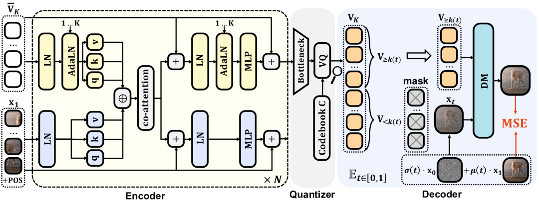
Figure 6: Selftok architecture diagram. $+\mathbf{POS}$: adding positional embeddings; $\mathbf{LN}$: layernorm; $\mathbf{AdaLN}$: token-aware adaptive layernorm, which differentiates token embeddings; $\mathbf{MSE}$: the mean squared error for the reconstruction objective; $\mathbf{DM}$: pre-trained diffusion model.

We use a dual-stream transformer backbone like MMDiT [24], which consists of an image stream (blue modules) and a token stream (yellow modules). Each stream has its own parameters, specialized for processing patch-based image embeddings and AR-based token embeddings. The backbone consists of $N$ blocks with identical architecture. We elaborate on our design choices below:

Input image. We use the pre-trained VAE of SD3 [24] to transform the images into VAE latent embeddings. This downscales an image (in pixel-wise RGB values) by a factor of 8, e.g., turning an image of size $256\times 256$ to a $32\times 32$ latent. We follow ViT [22] to patchify and flatten the latent into an $\mathbb{R}^{M\times D}$ sequence denoted as $\mathbf{x}_{1}$, where $M$ is $\#\textrm{patches}$ and $D=512$ is the embedding dimension. We add 2D sinusoidal positional embedding to the sequence before sending it to the image stream.

Input token. The token stream inputs a sequence of learnable continuous token embeddings $\overline{\mathbf{V}}_{K}\in\mathbb{R}^{K\times D}$, which is part of the model parameters and independent from $I$.

Co-attention. In each encoder block, the two streams interact through a co-attention, where their queries, keys, and values are concatenated to compute scaled dot-product attention. As the output of the image stream will not be input to the subsequent quantizer, to improve computational efficiency, we apply an attention mask that prevents queries from the image stream from attending to keys in the token stream. This reduces the attention computation, while still giving the token stream access to image features to complete the encoding.

Token-aware adaptive layernorm (AdaLN). Motivated by how MMDiT uses AdaLN to differentiate diffusion time-steps, our AdaLN uses token-aware scale and shift parameters $\boldsymbol{\alpha}_{k},\boldsymbol{\beta}_{k}\in\mathbb{R}^{D}$ for each token index $k\in\{1,\ldots,K\}$. Given an input token embedding $\mathbf{v}_{k}\in\mathbb{R}^{D}$, the AdaLN output is computed as $\boldsymbol{\alpha}_{k}\odot\mathrm{LN}(\mathbf{v}_{k})+\boldsymbol{\beta}_{k}$, where $\mathrm{LN}$ denotes layer normalization.

Output. After $N$ blocks, the input learnable token embeddings $\overline{\mathbf{V}}_{K}$ are eventually transformed into the $K$ continuous embeddings $\mathbf{V}=[\mathbf{v}_{1},...,\mathbf{v}_{K}]\in\mathbb{R}^{K\times D}$ as output. They are subsequently sent to the quantizer to obtain the $K$ discrete tokens $\mathcal{V}_{K}$. The output of the image stream is discarded.

2.2.2 Quantizer

The quantizer module consists of a bottleneck linear layer, followed by a vector quantization step using a learnable codebook. The bottleneck maps token embeddings $\mathbf{V}$ from $\mathbb{R}^{K\times D}\to\mathbb{R}^{K\times D^{\prime}}$, where $D^{\prime}=16<D$. The codebook has $C=2^{15}$ words and denoted as $\mathbf{C}\in\mathbb{R}^{C\times D^{\prime}}$. As illustrated in Figure 6, the bottleneck first compresses the token embeddings $\mathbf{V}$ from $\mathbb{R}^{K\times D}$ to $\mathbb{R}^{K\times D^{\prime}}$. Then, each $\mathbf{v}_{k}\in\mathbf{V}$ is quantized by assigning it to a codebook word $\mathbf{c}\in\mathbf{C}$ with the highest cosine similarity. Thus, the discrete token $v_{k}$ is the integer index of $\mathbf{c}$. The quantized embedding output is computed with the straight-through estimator [110] as $\mathbf{v}_{k}\leftarrow\mathbf{v}_{k}+(\mathbf{c}-\mathbf{v}_{k})\text{.detach}$, where “detach” cuts the gradient flow to $(\mathbf{c}-\mathbf{v}_{k})$ in backpropagation. This approximation ensures that the forward pass uses the quantized embedding $\mathbf{c}$, while the backward pass allows gradients to flow through $\mathbf{v}_{k}$ to the encoder.

Quantization loss. The quantization loss $\mathcal{L}_{Q}$ for learning the codebook $\mathbf{C}$ is:

$$\mathcal{L}_{Q}=\underbrace{\sum_{k=1}^{K}\|\mathbf{v}_{k}-\mathbf{c}_{k}\|^{2}}_{\text{commitment loss}}+\underbrace{\sum_{\mathbf{c}\in\mathbf{C}}\bar{p}_{\mathbf{c}}\mathrm{log}\;\bar{p}_{\mathbf{c}},}_{\text{entropy loss}}\text{where }\underbrace{\bar{p}_{\mathbf{c}}=\mathop{\mathbb{E}}_{\mathbf{V}\sim\mathcal{B}}\mathop{\mathbb{E}}_{\mathbf{v}_{k}\sim\mathbf{V}}\left[\frac{\mathrm{exp}(\mathrm{cos}(\mathbf{v}_{k},\mathbf{c})/\tau)}{\sum_{\mathbf{c}^{\prime}\in\mathbf{C}}\mathrm{exp}(\mathrm{cos}(\mathbf{v}_{k},\mathbf{c}^{\prime})/\tau)}\right]}_{\text{average assignment probability of word $\mathbf{c}$ in batch $\mathcal{B}$}},$$ (7)

where the temperature $\tau=0.1$. The commitment loss encourages each token embedding $\mathbf{v}_{k}$ to be close to its assigned word $\mathbf{c}_{k}$. The entropy loss encourages diverse codebook usage by promoting uniform word assignment, i.e., the average assignment probability $\bar{p}_{\mathbf{c}}$ of each word should be close to $1/C$. We compute $\bar{p}_{\mathbf{c}}$ in a batch $\mathcal{B}$ by averaging a soft assignment probability based on the cosine similarity $\mathrm{cos}(\mathbf{v}_{k},\mathbf{c})$ for each $\mathbf{v}_{k}\in\mathcal{B}$.

EMA update. Due to the non-differentiable nature of the quantizer, $\mathbf{C}$ is updated using an exponential-moving-average (EMA) to improve the training stability. For each sample batch, we compute a batch-specific centroid for each codebook word $\mathbf{c}\in\mathbf{C}$, defined as the mean embedding of all $\mathbf{v}_{k}$ that are assigned to the word. Let $\overline{\mathbf{C}}\in\mathbb{R}^{C\times D^{\prime}}$ denote the matrix of these centroids. The codebook update is: $\mathbf{C}\leftarrow\gamma\mathbf{C}+(1-\gamma)\overline{\mathbf{C}}$, where $\gamma=0.8$.

Dead-code reactivation. We observe that some codebook words may fall far from the token embedding distribution during early training and become underutilized. As a result, they rarely match with any $\mathbf{v}_{k}$. We identify such words by tracking the EMA of $\bar{p}_{\mathbf{c}}$ across batches, denoted as $\hat{p}_{\mathbf{c}}\leftarrow\eta\hat{p}_{\mathbf{c}}+(1-\eta)\bar{p}_{\mathbf{c}}$, where $\eta=0.99$. We mark $\mathbf{c}$ as dead code if its EMA $\hat{p}_{\mathbf{c}}$ falls below a threshold (we use $0.0125/C$). When this occurs, we reactivate $\mathbf{c}$ by assigning it to a randomly selected $\mathbf{v}_{k}$ from the current batch, pulling it back toward the active embedding space.

2.2.3 Decoder

Decoder architecture. Our $\mathrm{Dec}$ is a diffusion model initialized from SD3 [24]. It is a dual-stream transformer MMDiT architecture with the following customization: 1) Our token stream replaces the input of the original language token stream with the quantized embeddings $[\mathbf{v}_{k(t)},\ldots,\mathbf{v}_{K}]\in\mathbb{R}^{(K-k(t)+1)\times D^{\prime}}$ (the embeddings of $\mathcal{V}_{\geqslant k(t)}$) with 1D sinusoidal positional embedding; 2) To remove the original language influence and better adapt to Selftok tokens, the weights of our token stream are trained from scratch; 3) For the AdaLN layers in the image stream, we remove their dependency on the pooled CLIP text embedding and condition them only on the timestep $t$. For the token stream, we continue to use the token-aware AdaLN as in the encoder.

Overall objective. We jointly optimize the parameters of $\mathrm{Enc}$ (the combination of the encoder and the quantizer) and $\mathrm{Dec}$, using the objective below:

$$\mathop{\mathrm{min}}_{\begin{subarray}{c}\mathrm{Enc}(\mathbf{x}_{1})=\mathcal{V}_{K},\\ \mathrm{Dec}\end{subarray}}\leavevmode\nobreak\ \leavevmode\nobreak\ \mathop{\mathbb{E}}_{t\in[0,1]}\;\mathop{\mathbb{E}}_{\mathbf{x}_{0}\sim\mathcal{N}(0,1)}\left\|\mathbf{x}_{1}-\mathrm{Dec}\left((1-t)\cdot\mathbf{x}_{0}+t\cdot\mathbf{x}_{1},\mathbf{V}_{\geqslant k(t)}\right)\right\|^{2}+\mathcal{L}_{Q},$$ (8)

where $\mathbf{V}_{\geqslant k(t)}$ are the token embeddings of $\mathcal{V}_{\geqslant k(t)}$. We highlight the following details:
1) We uniformly sample $t\in[0,1]$, which yields the best performing model. We include ablation results in Section 2.3.2.
2) We follow SD3 to use the re-parameterization $\mathbf{x}_{t}=(1-t)\cdot\mathbf{x}_{0}+t\cdot\mathbf{x}_{1}$, i.e., $\sigma(t)=1-t$ and $\mu(t)=t$ in Eq. (6).
3) Before sending $\mathbf{V}_{\geqslant k(t)}$ to the decoder, we implement a re-weighting mechanism by updating each $\mathbf{v}_{k}$ as below:

$$\mathbf{v}_{k}\leftarrow\frac{\alpha}{p_{k}}\mathbf{v}_{k}+(\mathbf{v}_{k}-\frac{\alpha}{p_{k}}\mathbf{v}_{k}).\mathrm{detach},\;\text{where }p_{k}=\mathbb{E}_{t\in[0,1]}\mathbb{I}(v_{k}\in\mathcal{V}_{\geqslant k(t)}),$$ (9)

where $\alpha=0.5$ is is a weight constant, $p_{k}$ computes the probability of $v_{k}\in\mathcal{V}_{k(t)}$ for a uniformly sampled $t\in[0,1]$, and $\mathbb{I}(\cdot)$ is an indicator function. This re-weighting is introduced to correct the imbalance of $p_{k}$: as $k$ decreases, ${v}_{k}$ is more likely to be masked out by “$\geqslant$” in $\mathcal{V}_{\geqslant k(t)}$, resulting in smaller $p_{k}$ and fewer gradient updates on $\mathbf{v}_{k}$. By applying Eq. (9), the value of each embedding $\mathbf{v}_{k}$ remains unchanged in the forward pass, but in the backward pass, its gradient is scaled inversely to $p_{k}$ to compensate for the imbalanced $p_{k}$, i.e., $\mathbf{v}_{k}$ with fewer gradient updates is assigned with a larger gradient scale.
4) We discuss the choice of token schedule $k(t)$ below and include its ablation in Section 2.3.2.

2.2.4 Token Schedule

Recall that the AR constraint in Eq. (1) requires that every token must conform to the decomposition $P(\mathcal{V}_{K})\overset{\text{AR}}{=}P(\mathcal{V}_{<i})\cdot P(\mathcal{V}_{\geqslant i}|\mathcal{V}_{<i}),\forall i\in[1,K+1]$. We achieve this decomposition by diffusion time-steps, thanks to the recursive nature of the reverse diffusion process in Eq. (4), denoted as $\mathcal{V}_{\geqslant i}\Leftrightarrow\mathbf{x}_{t}\rightsquigarrow\mathbf{x}_{1}$ and $\mathcal{V}_{<i}\Leftrightarrow\mathbf{x}_{0}\rightsquigarrow\mathbf{x}_{t}$. That is to say, the second-half tokens $\mathcal{V}_{\geqslant i}$ can be learned recursively by the diffusion decoder, conditioned on $\mathbf{x}_{t}$, which represents the already identified first-half tokens $\mathcal{V}_{<i}$. As we uniformly sample $t\in[0,1]$ in training, the best token schedule should be a uniform assignment $k^{*}(t)=\left\lceil t\times K\right\rceil+1$ to ensure that every token is involved in the recursive diffusion time-step. To better understand this, we provide three failure cases:
1) If we allocate all the tokens to $\mathcal{V}_{\geqslant 1}$, i.e., $k(t)=1$, $\forall t\in[0,1)$, this corresponds to a trivial decomposition $P(\mathcal{V}_{<1}=[])\cdot P(\mathcal{V}_{K}|\mathcal{V}_{<1}=[])$, $\mathcal{V}_{K}\Leftrightarrow\mathbf{x}_{0}\rightsquigarrow\mathbf{x}_{1}$, and $[]\Leftrightarrow\mathbf{x}_{0}$, where we always input the full $\mathcal{V}_{K}$ to the decoder. So, $\mathcal{V}_{K}$ loses all the AR property. This case reduces to the FlowMo approach [93].
2) If we always allocate all tokens to $\mathcal{V}_{<1}$, i.e., $k(t)=K+1,\forall t\in(0,1]$, this corresponds to another trivial decomposition $P(\mathcal{V}_{K})\cdot P([]|\mathcal{V}_{K})$, $[]\Leftrightarrow\mathbf{x}_{0}\rightsquigarrow\mathbf{x}_{1}$, and $\mathcal{V}_{K}\Leftrightarrow\mathbf{x}_{0}$, where we always send an empty sequence to the decoder. This case reduces to the unconditional diffusion generation without learning $\mathcal{V}_{K}$ at all.
3) Consider a non-extreme case where $k(t)$ is not uniformly aligned with $t$, e.g., $k(t=0.8)=\left\lceil 0.2\times K\right\rceil$, we disrespect the decomposition because the majority of tokens $\mathcal{V}_{\geqslant\left\lceil 0.2\times K\right\rceil}$ corresponds to dense time-steps in the short interval $t\in[0.8,1]$, while the rest ones in $\mathcal{V}_{<\left\lceil 0.2\times K\right\rceil}$ corresponds to sparse time-steps, violating the balanced recursive correspondence in Eq. (4).

However, in practice, we empirically observe a better reconstruction quality by designing a schedule $k(t)$ that allocates fewer tokens to smaller $t$, i.e., $k(t)<k^{*}(t)$ for $t<0.5$. This aligns with the well-known trait of diffusion models: the early path $\mathbf{x}_{0}\rightsquigarrow\mathbf{x}_{t}$ for a small $t$ has minimal impact on the reconstruction $\mathbf{x}_{t}\rightsquigarrow\mathbf{x}_{1}$, which can be omitted [113, 82]. Nevertheless, identifying the optimal $k(t)$ that effectively balances the AR property and diffusion generation quality remains a challenging open problem, which we leave for future work.

2.2.5 One-step Renderer

As observed from the training objective in Eq. (8), Selftok tokens $\mathcal{V}_{K}$ participate in the reconstruction at every diffusion time-step. Hence after training, we can apply a standard multi-step diffusion sampler [24, 93] to decode $\mathcal{V}_{K}$ into a reconstructed image. However, this process is slow as it requires multiple sequential forward passes.

To accelerate this, we leverage the fact that $\mathcal{V}_{K}$ discretizes the entire generative path $\mathbf{x}_{0}\rightsquigarrow\mathbf{x}_{1}=I$, i.e., it encodes all the information of $I$, up to quantization loss. Hence, we aim to build a renderer $R(\mathcal{V}_{K})$ that reconstructs $I$ in a single forward pass. We initialize $R$ with the decoder weights optimized by Eq. (8). To remove its dependency on $\mathbf{x}_{t}$, we replace it with a sequence of learnable “canvas” token embeddings as shown in Figure 9 (b), which becomes part of the model parameters of $R$. Then with the learned token embeddings $\mathbf{V}_{K}=\mathrm{Enc}(I)$ frozen, we optimize $R$ jointly with an MSE loss for pixel-level reconstruction, LPIPS [131] and GAN [33] loss for perceptual quality, as including the latter two resolves the well-known blurry reconstruction issue when training a decoder with the MSE loss alone [55, 25]:

$$\mathop{\mathrm{min}}_{R(\mathbf{V}_{K})=I^{\prime}}\,\mathop{\mathrm{max}}_{D}\left[\underbrace{\|I-I^{\prime}\|^{2}}_{\text{MSE loss}}+\underbrace{\lambda_{1}\mathrm{LPIPS}(I,I^{\prime})}_{\text{perceptual loss}}+\underbrace{\lambda_{2}\left(\log D(I)+\log(1-D(I^{\prime})\right)}_{\text{GAN loss}}\right],$$ (10)

where $\lambda_{1},\lambda_{2}$ are loss weights, $D$ is the discriminator of the GAN. To improve training stability, we set $\lambda_{1}=0.1,\lambda_{2}=0$ for the first 30k training iterations and $\lambda_{1}=0.5,\lambda_{2}=0.5$ afterwards. As shown in Figure 9 (a), besides the improved visual perception, the one-step renderer brings two benefits: 1) it significantly reduces the image generation time, and 2) it eliminates the randomness introduced by the random seed in diffusion-based generation (see Figure 9 (a)). Explicit experimental results are shown in Section 2.3.2.

2.3 Validation

In this section, we empirically demonstrate that the Selftok tokenizer achieves the best reconstruction quality over all baselines in Section 2.3.1, while encoding tokens that satisfy the AR property (Figure 5). In addition, we provide comprehensive ablation studies in Section 2.3.2 to analyze various design choices, including #tokens $K$, codebook size $C$, token schedule $k(t)$, time-step sampler and the use of one-step renderer.

Settings. We used the train split of ImageNet-1k dataset [19] to train our tokenizer, where images were resized and center-cropped to the size of 256$\times$256. For evaluation, we used the validation split with the same image pre-processing. We evaluate the reconstruction quality using four metrics: 1) rFID [40] measures the dissimilarity between the distribution of reconstructed validation split and ground-truth train split; 2) PSNR measures a pixel-wise MSE between each image $I$ and its reconstruction $I^{\prime}$; 3) SSIM measures the perceptual similarity between $I$ and $I^{\prime}$ using a statistical approach [117]; 4) LPIPS does so by leveraging a pre-trained network [131].

2.3.1 Main Results

The results, presented in Table 1, show that Selftok achieves SoTA reconstruction performance (in terms of rFID, PSNR, SSIM, and LPIPS) and outperforms existing spatial tokenizers (both 1D and 2D, such as TiTok [128] and VAR [134]) as well as tokenizers using diffusion models as decoders, such as FlowMo [93]. Specifically, we can observe that when using 1024 tokens, existing tokenizers like Cosmos and FlowMo have worse reconstruction performance compared to ours (with a PSNR difference greater than 1). We also show the qualitative comparison between different tokenizers in Figure 7. Notably, we verify in Figure 2 that Selftok tokens are non-spatial by visualizing 1) progressive reconstruction by providing the decoder with an expanding sequence of tokens $\mathcal{V}_{\geqslant k(t)}$ for a decreasing $t$ from left to right, and 2) interpolation by gradually changing $\mathcal{V}_{\geqslant k(t)}$ for a decreasing $t$ of the left image with that of the right image. We further demonstrate the AR property of Selftok tokens in Figure 5.

Tokenizer	Type	#Token	#Code	rFID$\downarrow$	PSNR$\uparrow$	SSIM$\uparrow$	LPIPS$\downarrow$
LlamaGen [104]	2D	16$\times$16	$2^{14}$	2.19	20.67	0.589	0.132
MaskBiT†[119]	2D	16$\times$16	$2^{14}$	1.37	21.50	0.560	-
Cosmos [1]	2D	16$\times$16	$\approx 2^{16}$	4.40	19.98	0.536	0.153
VQGAN-LC† [134]	2D	16$\times$16	$100,000$	2.62	23.80	0.589	0.120
OpenMagViT-V2 [72]	2D	16$\times$16	$2^{18}$	1.17	21.63	0.640	0.111
ViT-VQGAN† [126]	2D	32$\times$32	$2^{13}$	1.28	-	-	-
LlamaGen [104]	2D	32$\times$32	$2^{14}$	0.59	24.44	0.768	0.064
Cosmos [1]	2D	32$\times$32	$\approx 2^{16}$	0.87	24.82	0.763	0.070
VAR [109]	2D	680	$2^{12}$	0.99	22.12	0.624	0.109
TiTok-L-32 [128]	1D	32	$2^{12}$	2.21	15.60	0.359	0.322
TiTok-B-64 [128]	1D	64	$2^{12}$	1.70	16.80	0.407	0.252
TiTok-S-128 [128]	1D	128	$2^{12}$	1.71	17.52	0.437	0.210
FlexTok [4]	1D	256	$64,000$	1.45	18.53	0.465	0.222
FlowMo-Lo† [93]	1D	256	$2^{18}$	0.95	22.07	0.649	0.113
FlowMo-Hi† [93]	1D	1,024	$2^{14}$	0.56	24.93	0.785	0.073
Selftok (Ours)	1D	512	$2^{15}$	0.70	24.14	0.709	0.084
Selftok (Ours)	1D	1,024	$2^{15}$	0.54	26.30	0.805	0.063

Table 1: Reconstruction performance of different tokenizers on $256\times 256$-resolution ImageNet 50k validation set. ^† Results from the original paper.

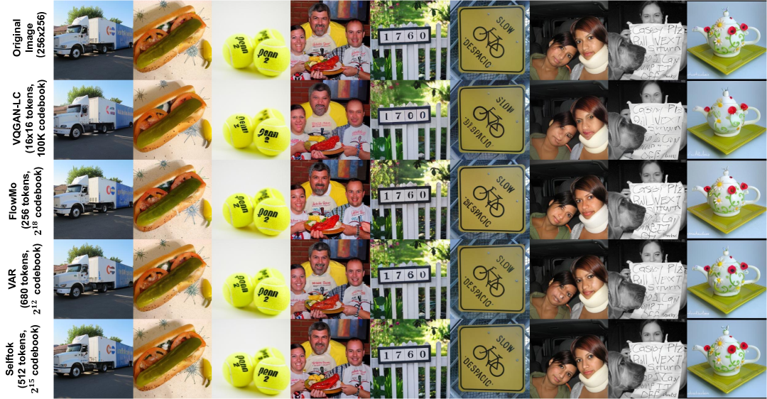
Figure 7: Comparison of reconstructions from different tokenizers.

2.3.2 Ablations

#Tokens $K$ and codebook size $C$. Increasing $K$ or $C$ trades off compression rate in favor of reconstruction quality. We verify this in Table 4 and Table 3, where we tried $K$ of 512 and 1,024, and $C$ of 32,768 ($2^{15}$) and 65,536 ($2^{16}$). For a lower compression rate, we chose $C$=32,768.

Time sampl.	Token sched.	PSNR$\uparrow$	SSIM$\uparrow$	LPIPS$\downarrow$
uniform	custom	21.86	0.600	0.150
uniform	uniform	21.10	0.564	0.177
uniform	logit-normal	20.78	0.555	0.180
logit-normal	custom	20.98	0.561	0.170
logit-normal	uniform	19.89	0.498	0.205
logit-normal	logit-normal	20.08	0.513	0.196

Table 2: Ablation on time sampler and token schedules. ‘sampl.’ and ‘sched.’ denote ‘sampler’ and ‘schedule’.

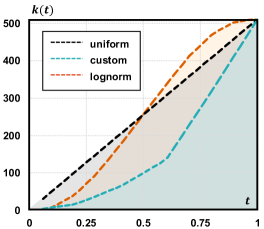
Figure 8: Token schedule $k(t)$. “lognorm” denotes logit-normal.

#Code	PSNR$\uparrow$	SSIM$\uparrow$	LPIPS$\downarrow$
$2^{15}$	21.86	0.600	0.150
$2^{16}$	22.12	0.618	0.135

Table 3: Ablation on the codebook size without one-step renderer.

Time sampler. For time sampler, besides the simple uniform sampling, SD3 [24] introduces the logit-normal time-step sampler by assigning higher probability density to mid-range time-steps ($t\approx 0.5$). We compared the reconstruction performance when using uniform and logit-normal sampling in Table 2, which shows that the simple uniform sampling performs the best for Selftok.

Token schedule $k(t)$. We explored three different choices for $k(t)$: 1) the uniform one with $k(t)=\left\lceil t\times K\right\rceil+1$; 2) a custom schedule that allocates few tokens to small $t$; and 3) a logit-normal schedule that allocates few tokens to both small and large $t$. We plot $k(t)$ in Figure 8 and compare the performance of the models trained with each schedule in Table 2. As we mentioned earlier in Section 2.2.4, our manually designed schedule wins as it aligns with the trait of diffusion models, i.e., $\mathbf{x}_{0}\rightsquigarrow\mathbf{x}_{t}$ for a small $t$ has minimal impact on reconstruction, hence tokens should be allocated elsewhere.

Model	Tokens	PSNR$\uparrow$	SSIM$\uparrow$	LPIPS$\downarrow$
Selftok w/o renderer	512	21.86	0.600	0.150
	1,024	23.06	0.670	0.119
Selftok w/ renderer	512	24.14	0.709	0.084
	1,024	26.26	0.805	0.063

Table 4: Ablation on the one-step renderer.

One-step Renderer. We trained a one-step renderer with Eq. (10) to further accelerate the image reconstruction process. With the one-step renderer, the reconstruction time decreases from 8.2 sec/per image to 0.31 sec/per image (the reconstruction time is tested in one Huawei Asecnd 910B2 with batchsize $=1$). Additionally, the reconstruction performance improves, as shown in Table. 4 and we also present some qualitative results before and after using the one-step renderer in Figure 9 (b). One-step render helps both accelerate the reconstruction speed and improves the reconstruction quality in a large scale.

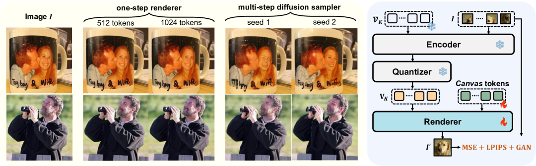
Figure 9: Left: (a) Reconstructions with one-step renderer (512 or 1024 tokens) and multi-step diffusion sampler (512 tokens, two seeds); Right: (b) Renderer architecture diagram.

3 Selftok-based VLM

Thanks to the Selftok tokenizer, images can be encoded into discrete token sequences, which are then processed by a single, purely discrete AR model for visual generation and reasoning. Each visual token sequence can be decoded back into pixel space using the one-step renderer. In Section 3.1, we show the model architecture and training strategy of VLM. Then we present validation results in Section 3.2.

3.1 Training

We initialize the VLM from the pretrained Llama3-8B [2] model and expand its vocabulary with an additional 32,768 Selftok visual words. As a result, the model’s vocabulary integrates both textual and visual tokens into a unified embedding space. As illustrated in Figure 1, the VLM is trained using the standard language modeling objective, which aims to maximize the log-likelihood of multimodal token sequences in an AR fashion:

$$P(\mathcal{Y})=\sum_{i=1}^{|\mathcal{Y}|}\log P_{\theta}(y_{i}|\mathcal{Y}_{<i}),$$

where the sequence $\mathcal{Y}$ may consist of interleaved language and visual tokens, and thus $y_{i}\in\mathcal{Y}$ denotes either a language token $\langle w_{i}\rangle$ or a visual token $\langle v_{i}\rangle$. Since both text and image content are represented as discrete token IDs, the prediction head is shared and supervised at each position using a cross-entropy loss. The training consists of the following two stages:

Stage1: Cross-modality Alignment. In this stage, we aim to learn the alignment between visual tokens and language tokens, thereby facilitating the transition of the pre-trained Llama3 model from LLM to VLM. To achieve this, we introduce four data formats designed to address the challenges of cross-modality alignment. Each format helps the model process and integrate vision and language inputs for coherent multimodal understanding and generation. The Text-to-Image format aligns caption with visual data, enabling image generation from textual descriptions. Conversely, the Image-to-Text format facilitates understanding tasks by associating visual data with textual descriptions. To address potential misalignments that can occur during text-to-image tasks, the Image-Only format is introduced, allowing the model to learn visual structure independently. Finally, the Text-Only data ensures the preservation of the model’s linguistic capabilities, maintaining its ability to process and generate text. These formats and their functions are summarized in Figure 11, with special tokens such as [BOS] and [EOS] marking the sequence boundaries, and [BOV] and [EOV] indicating the start and end of visual data. The training data is comprised of 530 million high-quality image-text pairs and text sequences (See Appendix for more details).

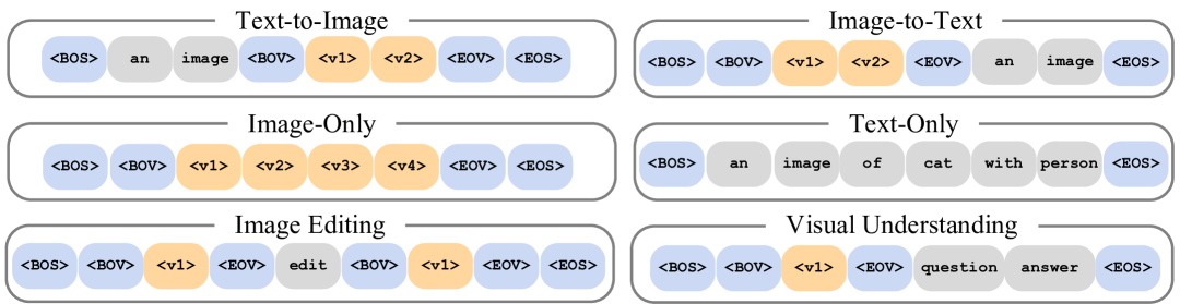
Figure 10: Illustration of the proposed data format for cross-modality and cross-task alignment.

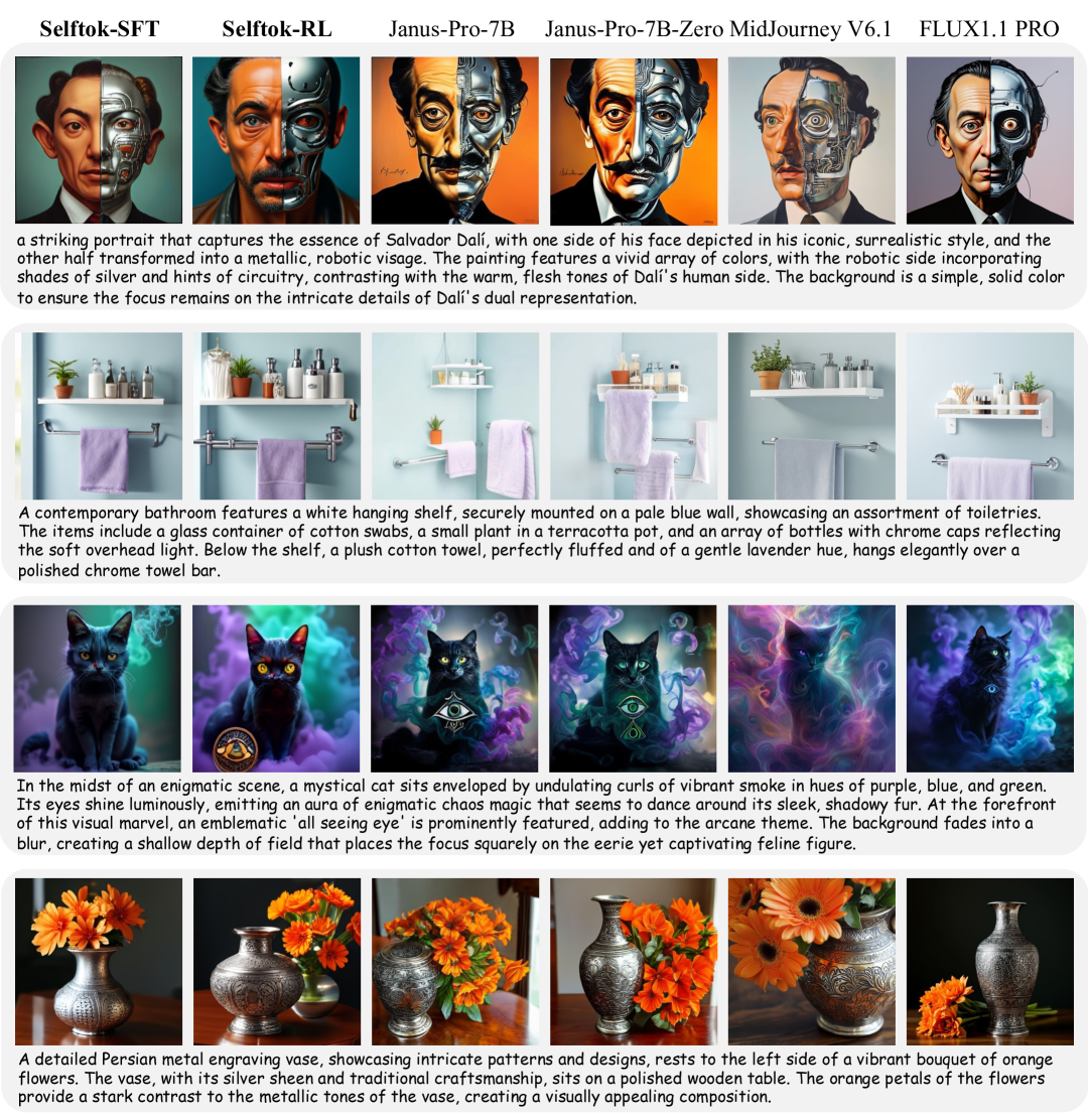
Figure 11: Text-to-Image generation results by Selftok using the text prompts of DPG-Bench.

Stage2: Cross-task Alignment. In this stage, we perform cross-task alignment to enable the model to learn human instructions across various tasks. This is accomplished through supervised fine-tuning (SFT) on datasets from three distinct tasks: 1) text-to-image generation, 2) image editing, and 3) image understanding. The instruction format follows the structure ‘‘USER: <Instructions> ASSISTANT: <Answers>’’, where only the content of <Answer> contributes to the loss function, optimizing the model’s ability to provide accurate responses. Detailed data organization and training details are provided in the Appendix.

3.2 Validation

After completing the two stages of training, we evaluated the model’s performance on three downstream tasks: text-to-image generation, image editing, and image understanding. During inference, we introduced logit adjustment to improve model performance. The adjustment is applied when the entropy of the conditional logits exceeds a threshold $\tau$, indicating that the model is uncertain about the current token:

$$\text{logit}_{\text{adjusted}}=\begin{cases}\text{logit}_{c}+(\gamma-1)\cdot(\text{logit}_{c}-\text{logit}_{u}),&\text{if}\;H(\text{logit}_{c})>\tau\\ \text{logit}_{c},&\text{otherwise}\end{cases}$$ (11)

By mitigating this uncertainty, the adjustment strengthens the model’s performance across diverse tasks. Logit_c and logit_u represent the logits predicted by the model for each token in the autoregressive sequence generation process. For text-to-image generation, $\text{logit}_{c}$ refers to the output with text prompt input, while $\text{logit}_{u}$ refers to the output with a null prompt. For image editing, $\text{logit}_{c}$ refers to the output with both text instruction and image input, while $\text{logit}_{u}$ refers to the output with only image input (no text instruction).

It is important to note that language AR models do not require logit adjustment, while Selftok does. This is due to resource limitations, as the current VLM is relatively small in scale and has not undergone pretraining on the visual modality, which leads to high entropy at certain timesteps due to dataset bias [80, 79]. However, this issue can be mitigated through future large-scale visual pretraining using videos [67].

Method	T2I Model	Structure Distance ↓	Background Preservation				CLIP Similarity
			PSNR ↑	LPIPS ↓	MSE ↓	SSIM ↑	Whole ↑	Edited ↑
Prompt-to-Prompt [39]	SD1.4	69.43	17.87	208.80	219.88	71.14	25.01	22.44
Null-text Inversion [78]	SD1.4	13.44	27.03	60.67	35.86	84.11	24.75	21.86
PnP Inversion [53]	SD1.4	11.65	27.22	54.55	32.86	84.76	25.02	22.10
Pix2Pix-Zero [85]	SD1.4	61.68	20.44	172.22	144.12	74.67	22.80	20.54
MasaCtrl [8]	SD1.4	28.38	22.17	106.62	86.97	79.67	23.96	21.16
InstructPix2Pix [6]	SD1.5	107.43	16.69	271.33	392.22	68.39	23.49	22.20
MagicBrush [130]	SD1.5	26.81	26.85	66.67	171.11	83.37	23.89	20.84
InstructDiffusion [30]	SD1.5	74.21	20.88	142.35	353.45	76.70	24.06	21.57
MGIE [26]	SD1.5	67.41	21.20	142.25	295.11	77.52	24.28	21.79
SEED-X-Edit [29]	SD-XL	61.69	18.80	173.63	209.05	74.93	25.51	22.20
EditAR [79]	LlamaGen	39.43	21.32	117.15	130.27	75.13	24.87	21.87
Selftok (Ours)	Llama3.1	35.89	23.76	124.48	76.78	78.46	24.94	22.02

Table 5: Quantitative comparison on PIE-Bench dataset [53] with various single-image inversion-based methods (top) and large-scale training approaches (bottom). Among the large-scale training ones, EditAR [79] is an autoregressive framework.

3.2.1 Text-to-Image Generation

Metric Evaluation. To evaluate the performance of our model, we conduct tests on two widely-used benchmarks: GenEval [31] and DPG-Bench [47]. The evaluation results are shown in Tables 7 and 8, respectively, which incorporate both stages of the model training: cross-modality training (Selftok-Pre) and cross-task training (Selftok-SFT). On the GenEval benchmark, Selftok-Pre achieves a score of 0.60, outperforming Emu3-Gen (0.54) and TokenFlow (0.55). After SFT, the score of our model increases to 0.74, surpassing Infinity (0.73) and CogView4 (0.73). Similarly, Selftok-SFT reaches 81.8, exceeding Emu3-Gen (80.6) on the DPG benchmark. This highlights that our model enables better image-text alignment.

Qualitative Examples. In Figure 11, we visualize the performance of Selftok on the DPG test prompt. We also compare our model with MidJourney and FLUX [57], showing that Selftok performs well in both adhering to complex semantics and generating aesthetically pleasing images. However, it should be noted that the current model can only generate images at a resolution of $256\times 256$, indicating significant potential for improvement in image detail in future work.

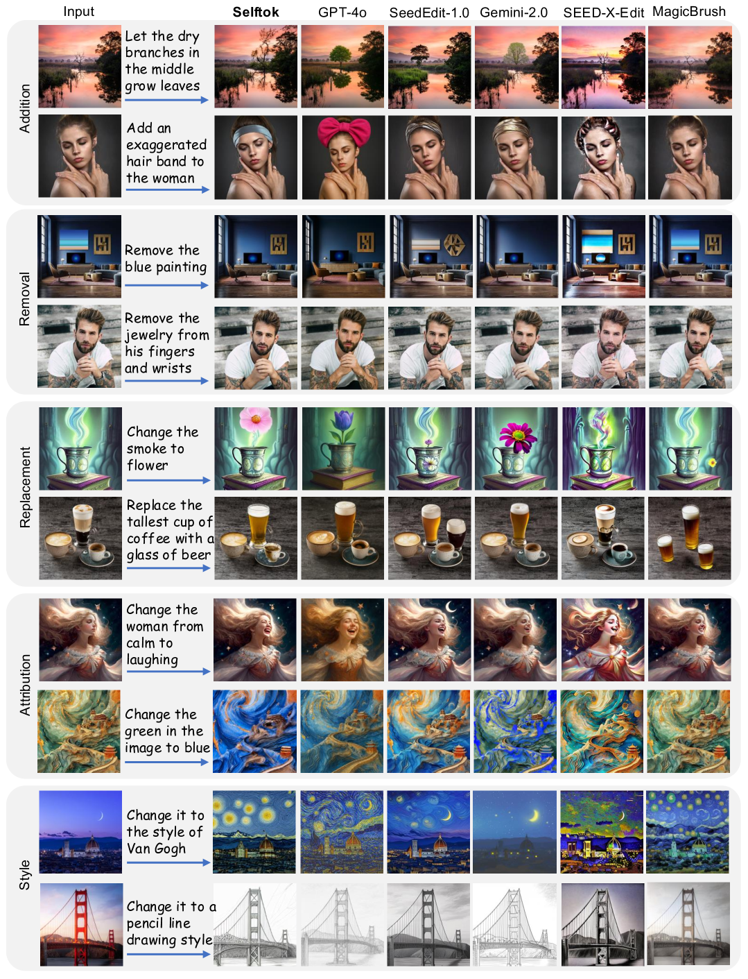
Figure 12: Qualitative comparison on single-turn editing across five editing types.

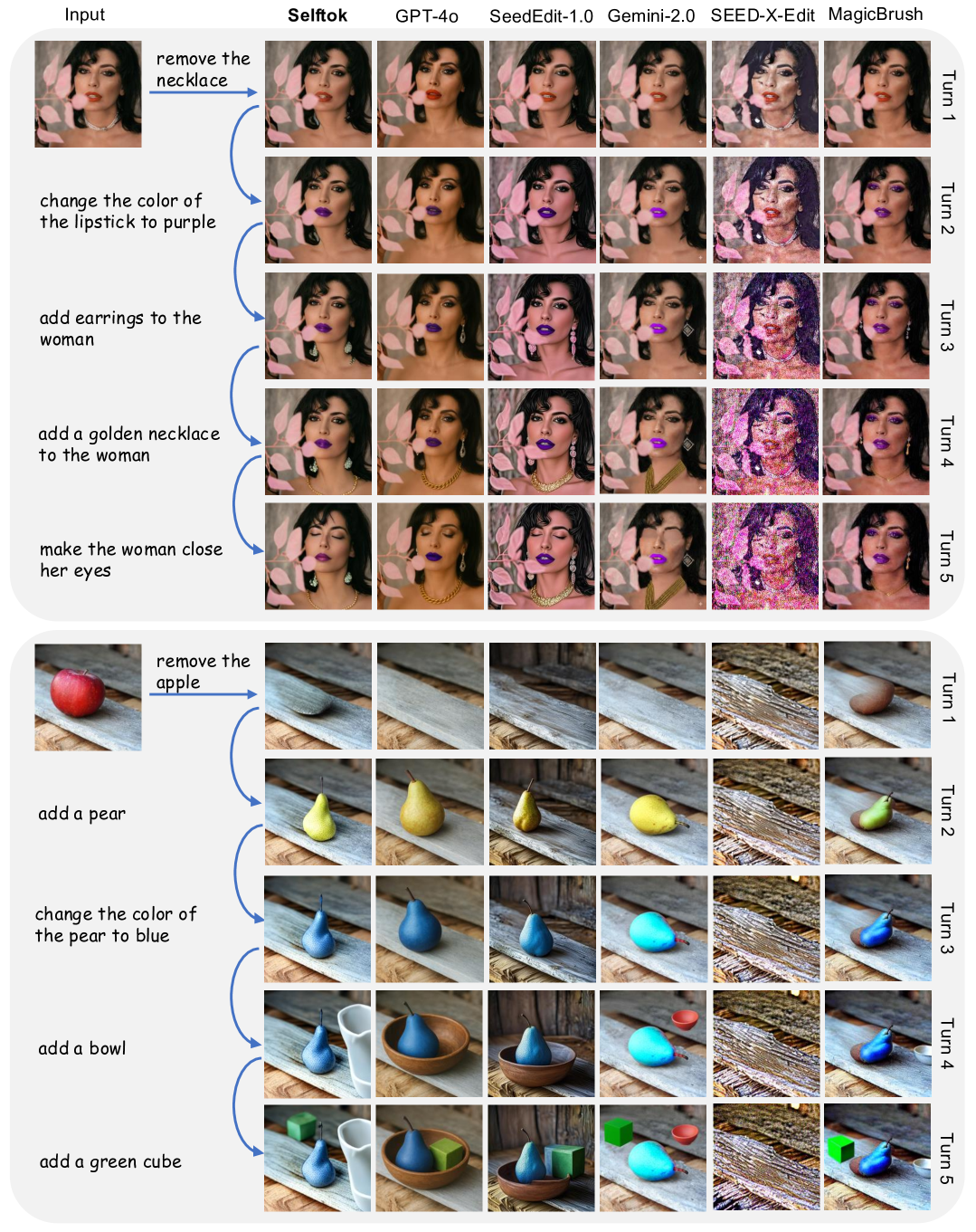
Figure 13: Qualitative comparison on multi-turn editing.

3.2.2 Image Editing

Metric Evaluation. In Table 5, we conduct a quantitative comparison with previous single-image inversion-based methods and large-scale training ones. Specifically, Structure Distance and Background Preservation metrics reflect fidelity while CLIP Similarity is adopted for evaluating editability. Among the inversion methods, optimization-based approaches, i.e., Null-text Inversion [78] and PnP Inversion [53] achieve relatively better fidelity and editability. However, they are time-consuming during test time. For large-scale training approaches, MagicBrush [130] obtains the best fidelity but the worst editability. By contrast, SEED-X-Edit [29] exhibits the best performance in editability and is worse in fidelity. They fail to achieve a good balance between these two. Served as an autoregressive framework, EditAR [79] shows a better trade-off. In comparison with EditAR [79], our Selftok excels in most metrics and obtains the best results on the PIE-Bench dataset [53]. It is worth noting that a standardized and objectively reliable evaluation metric for editing has yet to be established in our community. As a result, human evaluation remains the de facto “gold” standard.

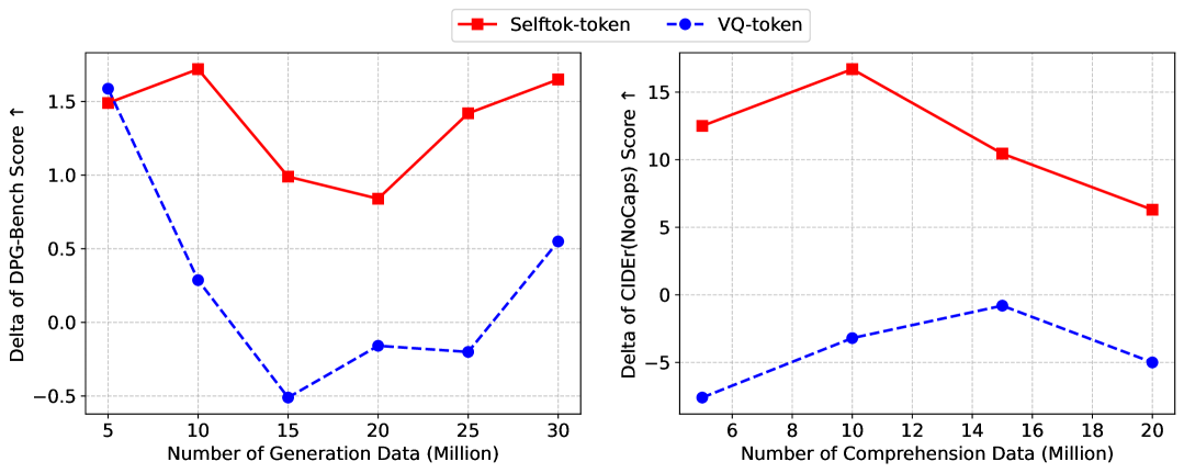
Figure 14: Synergy comparison between Selftok and spatial VQ-tokens. $\Delta$ is computed as the performance gain from dual-task training over single-task training. Left: Generation task performance (DPG-Bench). Right: Comprehension task performance (NoCaps).

Qualitative Examples. To have a comprehensive evaluation of our Selftok, we perform a qualitative comparison with leading works, i.e., GPT-4o, SeedEdit-1.0 [99], Gemini-2.0, SEED-X-Edit [29], and MagicBrush [130], on both single-turn and multi-turn editing. For the comparison of single-turn editing across five editing types in Figure 12, GPT-4o, SeedEdit-1.0 [99], and Gemini-2.0 achieve better performance considering both the fidelity and editability. It could be seen that our Selftok gets comparative results with these three. Figure 13 gives two examples of multi-turn editing with five turns. Among the compared methods, GPT-4o exhibits the strongest editing capability in the multi-turn setting. Our Selftok demonstrates relatively better performance in terms of text-image alignment and identity preservation across all turns.

3.2.3 Vision-Language Comprehension

Metric Evaluation. We evaluate the models on the visual comprehension benchmark MME, comparing two main categories of methods: “Specialized Visual Understanding MLLMs” and “MLLMs for both Visual Understanding and Generation”. As shown in Table 6, Selftok achieves a score of 1381.3, outperforming methods that jointly perform generation and understanding (e.g., Emu3 with 1292.8 and VILA-U with 1338.1). However, it still falls short of models specifically designed for comprehension tasks, such as LLaVA (1532.1); or those equipped with an additional comprehension branch, such as Janus-Pro (1576.0). This discrepancy can be attributed to the lack of specialized data for training on comprehension tasks. Recent studies have demonstrated the effectiveness of RL in enhancing vision-language comprehension tasks [98, 87, 50]. Recall that comprehension tasks produce only language outputs; therefore, these RL methods can be regarded as natural extensions of the success of RL in LLMs and thus fall outside the scope of this work. In contrast, we argue that RL for visual generation remains largely underexplored and presents unique challenges, which we examine in greater detail in Section 4.

Type	Method	#Params	Exist.	Count	Pos.	Color	Poster	Celeb.	Scene	Landm.	Art.	OCR	Total
Und. Only	InstructBLIP [17]	13B	185.0	143.3	66.7	153.3	123.8	101.2	153.0	79.8	134.3	72.5	1212.8
	Qwen-VL-Chat [5]	7B	158.3	150.0	128.3	170.0	178.6	120.6	152.3	164.0	125.5	140.0	1487.6
	LLaVA-v1.5 [66]	7B	185.0	155.0	133.3	170.0	160.5	152.9	161.2	170.5	118.8	125.0	1532.1
	InternVL-Chat-V1.5 [15]	20B	190.0	175.0	166.7	178.3	173.8	138.5	154.8	177.8	143.0	140.0	1637.8
	InternLM-XComposer2-VL [21]	7B	195.0	160.0	163.3	195.0	171.1	153.8	164.8	176.0	185.5	147.5	1712.0
Und. & Gen.	Show-o [124]	1.3B	190.0	103.3	106.7	170.0	46.9	53.8	156.5	116.5	102.0	57.5	1103.3
	Emu3 [116]	8B	200.0	145.0	146.7	170.0	109.5	79.4	157.2	121.0	94.0	70.0	1292.8
	VILA-U [123]	7B	165.0	136.7	121.7	158.3	127.9	106.8	160.2	151.2	122.8	87.5	1338.1
	Liquid [122]	7B	163.3	96.7	115.0	133.3	75.5	84.1	140.0	82.5	86.0	55.0	1031.5
	Janus-Pro [13]	7B	185.0	161.7	128.3	175.0	152.4	159.4	163.5	157.8	123.0	170.0	1576.0
	Selftok	8B	180.0	116.7	118.3	175.0	122.8	121.5	161.5	176.8	91.3	117.5	1381.3

Table 6: Comparison for multimodal comprehension on MME vision-language benchmarks. All the unified model scores are reproduced using the official open-source code, as the original papers do not provide scores for individual components.

Synergy between Generation and Comprehension: The synergy of visual comprehension and generation is challenging because of the conflicting objectives [84]: for comprehension, the VLM needs to abstract the visuals (invariance); for generation, it needs to preserve the visuals as much as possible (equivariance). We conduct ablation experiments and introduce the following metric:

$$\Delta=\text{Performance}_{\text{(Both Tasks)}}-\text{Performance}_{\text{(Single Task)}},$$ (12)

where “Both Tasks” refers to training on understanding and generation with a fixed data ratio (i.e., 4:6), and “Single Task” refers to the generation or the comprehension, as shown in Figure 14. We visualize the results for different amounts of generation data to mitigate the risk of underfitting. The results demonstrate that Selftok consistently outperforms spatial tokens (the VQToken adopted in [13]), with $\Delta$ remaining positive across all data levels, highlighting a clear synergy between understanding and generation tasks. In contrast, the spatial tokens exhibit negative $\Delta$ values at certain points, suggesting a conflict. Note that this synergy holds great potential for post-training in vision-language models (VLMs), as comprehension must be used as the reward model to guide reinforcement learning for visual generation (Section 4.2.1).

4 Selftok-based Visual RL

There is no universally “correct” ground-truth label for multimodal alignment. For instance, a single text prompt in text-to-image generation may correspond to infinitely many plausible images. Consequently, a VLM trained solely on vision-language pairs tends to naively mimic the training distribution rather than perform genuine reasoning, resulting in the well-known hallucination issue [71, 61, 111]. This is shown in Figure 17, where the Selftok-SFT model cannot generate “yellow broccoli” or “red dog” due to the rare combinations in training data (see Appendix B. Selftok-based Visual RL for more details). A straightforward remedy is to curate a supervised dataset that exhaustively covers all possible alignments. However, this approach is unsustainable.

This motivates us to the need for visual reinforcement learning (visual RL), a paradigm that visual generative models are trained without ground-truth images, relying instead on task-specific rewards, such as the CLIP-based image-prompt similarity [90] for text-to-image generation. Inspired by the success of RL in LLMs, which unlocks their reasoning capabilities, we believe that visual RL can similarly advance visual generation from mere imitation to genuine reasoning.

Next, we formulate the problem of visual RL in Section 4.1, which reveals that AR tokens are necessary in this setup. In Section 4.2, we design an RL training pipeline for Selftok. Thanks to its AR property, we show in Section 4.3 that this leads to significant improvements in GenEval and DPG-Bench, which are not yet observed for non-AR spatial tokens.

4.1 Problem Formulation

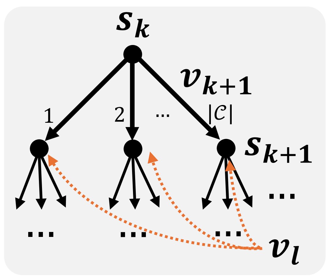
Figure 15: The recursive Bellman equation fails when a child node $v_{l}$ (i.e., future token) anti-causally affects a parent node $v_{k+1}$.

In visual RL, we aim to fine-tune a VLM (policy) that selects the next token (action) based on the current sequence (state) to maximize a task-specific reward (e.g., the consistency between the text prompt and generated image). Without loss of generality, we limit our discussion to visual tokens $[v_{1},\ldots,v_{K}]$, as the same principle applies to language tokens. We discuss the recipe for visual RL in detail:
1) State: The state $s_{k}=[v_{1},\ldots,v_{k}]$ is the token sequence generated by VLM at step $k\in\{1,\ldots,K\}$, and the initial state $s_{0}=[]$ is defined as an empty sequence.
2) Action: An action at step $k$ selects the next token $v_{k+1}$ from the visual codebook $\mathcal{C}$, i.e., at each step, there are $|\mathcal{C}|$ possible actions to choose from.
3) State transition: $P(s_{k+1}|s_{k},v_{k+1})=1$ because $s_{k+1}=[s_{k},v_{k+1}]$.
4) Reward: Generally, the reward $r(s_{k},v_{k+1})$ received at step $k+1$ depends on the previous state $s_{k}$ (where the reward is from) and the action as the next token $v_{k+1}$, predicted at the previous state (how the reward is obtained). With the state and action defined above, $s_{k+1}=[s_{k},v_{k+1}]$, we can also write $r(s_{k+1})=r(s_{k},v_{k+1})$.
5) Policy: Given the current state $s_{k}$, the policy $\pi(v_{k+1}|s_{k})$ predicts an action as the next token $v_{k+1}$. The goal of RL is to find an optimal policy $\pi$, which generates a trajectory $s_{0}\rightsquigarrow s_{K}$ that maximizes the cumulative reward (with omitted discount factor):

$$\mathop{\mathrm{max}}_{\pi}V_{\pi}(s_{0}),\quad\text{where}\quad V_{\pi}(s_{k})=\mathbb{E}_{\pi}\left[\sum_{i=k}^{K-1}r(s_{i},v_{i+1})\right].$$ (13)

$V_{\pi}(s_{k})$ is the value function, accounting for the expectation of all the possible cumulative rewards received along the trajectory $s_{k}\rightsquigarrow s_{K}$ generated by $\pi$.

We now show that only AR tokens can derive the Bellman equation, which underpins the optimality of policy update that guarantees effective RL. We start by rewriting our goal $V_{\pi}(s_{0})$ in Eq. (13):

$$V_{\pi}(s_{0}) =\mathop{\mathbb{E}}_{[v_{1}\sim\pi(\cdot|s_{0}),v_{2}\sim\pi(\cdot|s_{1}),\ldots,v_{K}\sim\pi(\cdot|s_{K-1})]}\left[r(s_{0},v_{1})+r(s_{1},v_{2})+\ldots+r(s_{K-1},v_{K})\right]$$ (14)

$$=\mathop{\mathbb{E}}_{v_{1}\sim\pi(\cdot|s_{0})}r(s_{0},v_{1})+\mathop{\mathbb{E}}_{v_{1}\sim\pi(\cdot|s_{0})}\underbrace{\mathop{\mathbb{E}}_{[v_{2}\sim\pi(\cdot|s_{1}),\ldots,v_{K}\sim\pi(\cdot|s_{K-1})]}\left[r(s_{1},v_{2})+\ldots+r(s_{K-1},v_{K})\right]}_{V_{\pi}(s_{1})}$$ (15)

$$=\sum_{v_{1}\in\mathcal{C}}\pi(v_{1}|s_{0})\cdot\left[r(s_{1})+V_{\pi}(s_{1})\right].$$ (16)

Eq. (14) holds because the transition probability $P(s_{k+1}|s_{k},v_{k+1})=1$. As shown in Figure 15, Eq. (15) holds because of the causal dependency of AR, where the choice of action $v_{k+1}$ only depends on $s_{k}$ and does not affect the former action $v_{k}$ that has already been chosen. Therefore, we can recursively apply Eq. (16) and derive the Bellman equation:

$$V_{\pi}(s_{k})=\sum_{v_{k+1}\in\mathcal{C}}\pi(v_{k+1}|s_{k})\cdot\left[r(s_{k+1})+V_{\pi}(s_{k+1})\right].$$ (17)

Thanks to the above equation, the optimized $\pi$ in Eq. (13) can be step-by-step obtained:

$$\mathop{\mathrm{argmax}}_{v_{k+1}}\pi^{\prime}(v_{k+1}|s_{k})\leftarrow\mathop{\mathrm{argmax}}_{v_{k+1}}\left[r(s_{k+1})+V_{\pi}(s_{k+1})\right].$$ (18)

Although the above policy update is greedy, its optimality is guaranteed by the policy improvement theorem [106], which shows that the locally optimal action $v_{k+1}$ at step $k$ does not affect the earlier improved actions due to the AR property. Note that non-AR spatial tokens cannot satisfy the Bellman equation, and therefore cannot support the policy update that relies on it. The key reason is that Eq. (15) cannot be derived, as the future action $v_{l}$, where $l>k+1$, influences earlier actions through the anti-causal links (shown red in Figure 15). Therefore, spatial tokens are not compatible with RL.

4.2 Implementation

We now describe the implementation details for Selftok-based visual RL for visual generation, such as text-to-image and visual editing tasks, without using any pairwise supervision, including two reward models for evaluating the quality of the generated images and training objectives for updating the policy network.

4.2.1 Reward Model

The overall design philosophy of our reward model is to utilize visual comprehension models to evaluate the generated image in visual RL and provide feedback for optimization. For tasks such as text-to-image generation, the comprehension model should understand and evaluate the consistency between the generated image and the textual prompt. In this paper, we categorize the comprehension-based reward into two major types:
Program-based Reward: This type is useful for more structured tasks like object identification, counting, and spatial relationships [31], where the prompt explicitly and unambiguously states the desired generation, e.g., “3 clocks and 1 dog”, and thus we can use visual detectors [11] to evaluate the generation quality. For example, we count the clocks based on the detector’s confidence, returning 1 if the count is correct and 0 otherwise. Each prompt has its own item sets to be tested, and the average of the scores for each test is used as the reward score.
QA-based Reward: For more complex and ambiguous prompts, it is challenging to rely solely on automated programs. To this end, we resort to more powerful visual comprehension models like InternVL [15] or GPT-4o [52], which can comprehend nuanced prompts and generate accurate answers. Specifically, inspired by [16], we first decompose the prompt to semantic tuples (e.g., entity, attribute, and relation) and then generate questions (e.g., “Is the car red?”). The MLLMs are asked to perform a VQA task for the prompt and generated image, returning a score of 0 to 1 (e.g., wrong to correct) for each question. The reward is obtained by averaging the evaluation of the MLLMs on multiple questions for a prompt. We can also fine-tune such models to obtain more task-specific reward functions.

As a preliminary study, we only validate the feasibility of the above two types. However, we believe that there should be more effective comprehension tasks as reward models for better performance, and we leave the exploration of them for future work.

4.2.2 Policy Gradient

We adopt a simplified version of GRPO [97] without importance sampling and encourage readers to explore more advanced alternatives. For each prompt, the policy network $\pi$ generates a batch of outputs $\{s^{i}\}_{i=1}^{B}$, where $B$ represents the batch size and each $s^{i}$ denotes the final state $[v_{0},v_{1},\ldots,v_{K}]$ of the $i$-th visual sequence. For a batch, we calculate the total rewards $\{r(s^{i})\}_{i=1}^{B}$, where we slightly abuse the notation that the total reward $r(s^{i})=r(s_{K}^{i})$ as all the intermediate rewards $r(s_{k}^{i})=0$, $\forall k<K$. We also calculate the advantages $\{A_{i}\}_{i=1}^{B}$, where each $A_{i}$ measures the relative quality of output $s^{i}$ compared to the average reward:

$$A_{i}=\frac{r(s^{i})-\text{mean}(\{r(s^{1}),r(s^{2}),\ldots,r(s^{B})\})}{\text{std}(\{r(s^{1}),r(s^{2}),\ldots,r(s^{B}))},$$ (19)

where $\text{mean}(\cdot)$ and $\text{std}(\cdot)$ are the mean and standard deviation of all rewards, respectively.

Then, we update the policy network parameters by the following training loss:

$$\mathcal{L}=-\frac{1}{B}\sum_{i=1}^{B}\left[A_{i}-\lambda\mathbb{D}_{KL}(\pi||\pi_{\text{old}})\right],$$ (20)

where the KL divergence $\mathbb{D}_{KL}(\pi||\pi_{\text{old}})=\frac{\pi_{\text{old}}}{\pi}-\text{log}\frac{\pi_{\text{old}}}{\pi}-1$ is to maintain training stability. It measures the difference between the new policy $\pi$ and the old policy $\pi_{\text{old}}$, where the new policy $\pi$ is the up-to-date one after policy gradient; the old policy $\pi_{\text{old}}$ refers to the one used to generate the token sequences before the policy gradient update.

Difference from diffusion-based DPO. Direct Preference Optimization (DPO) in diffusion models [112] has long been mistakenly regarded as a visual RL method. Compared to our Selftok-based visual RL—which aligns with the standard formulation of RL in LLMs—the diffusion-based DPO essentially degenerates to contrastive learning between the “good” and “bad” explored samples. This limitation arises because diffusion models do not have access to the actual generation trajectories of the samples, i.e., they lack the state-action trajectories available in the original DPO formulation for LLMs [92]. In contrast, Selftok discretizes the entire diffusion generation path of an image, thereby encoding a complete state-action trajectory.

4.3 Validation

In this section, we experimentally evaluate the text-to-image generation capabilities of the Selftok-based AR model, demonstrating the effectiveness of visual RL. We also provide details of the visual RL training and analyze the impact of various factors on the model performance.

4.3.1 Implementation details

Based on the SFT model (see Section 3), we further apply the reward model (see Section 4.2.1) for visual RL and evaluate its performance on Geneval [31] and DPG-Bench [48].

For program-based reward, we use MM-Detection [11] as the detectors and set the threshold for detection to 0.6. For QA-based reward, we utilize InternVL [15] and mPLUG [59] as the comprehension model. Note that we carefully deduplicate the training prompts to ensure that there is no overlap with the test set. For the sake of reproducibility, after the visual RL training, we do not incorporate any test-time scaling techniques during inference.

4.3.2 Main Results

The quantitative experimental results are summarized in Table 7 and Table 8, which evaluate the performance of our Selftok-based approach on the GenEval and DPG-Bench benchmarks. Specifically, Selftok-Pre and Selftok-SFT refer to the models after stage 1 (cross-modality alignment) and stage 2 (cross-task alignment), respectively (see Section 3.1), while Selftok-Zero refers to the model after visual reinforcement learning (see Section 4.2).

Selftok-Zero achieves state-of-the-art performance in text-to-image generation. As shown in Table 7, Selftok-Zero obtains the highest overall score of 95 on the GenEval benchmark, surpassing all previous models, including strong baselines such as CogView4-6B (73) and HiDream-I1 (83). Selftok-Zero also outperforms across all major sub-tasks, e.g., Colors (97) and Position (98). Similarly, on DPG-Bench (Table 8), Selftok-Zero achieves an overall score of 85.57, outperforming SD3-Medium (84.08) and Janus-Pro-7B (84.19). The qualitative results are presented in Figure 17, the images generated by Selftok-Zero exhibit high-quality alignment with the textual descriptions.

Visual RL significantly enhances image-text consistency. A direct comparison of Selftok-SFT vs Selftok-Zero and Janus-Pro-7B^† vs Janus-Pro-7B-Zero highlights the benefits of visual RL. On GenEval, Selftok-Zero improves upon its supervised counterpart in nearly every metric, with notable gains in Position (45$\rightarrow$98) and Counting (66$\rightarrow$90). On DPG-Bench, visual RL leads to a +3.77 increase in overall score, with improvements in Entity (from 88.15$\rightarrow$91.78) and Relation (from 93.68$\rightarrow$95.26). These results indicate that visual RL is effective in closing the gap between generated images and complex textual prompts.

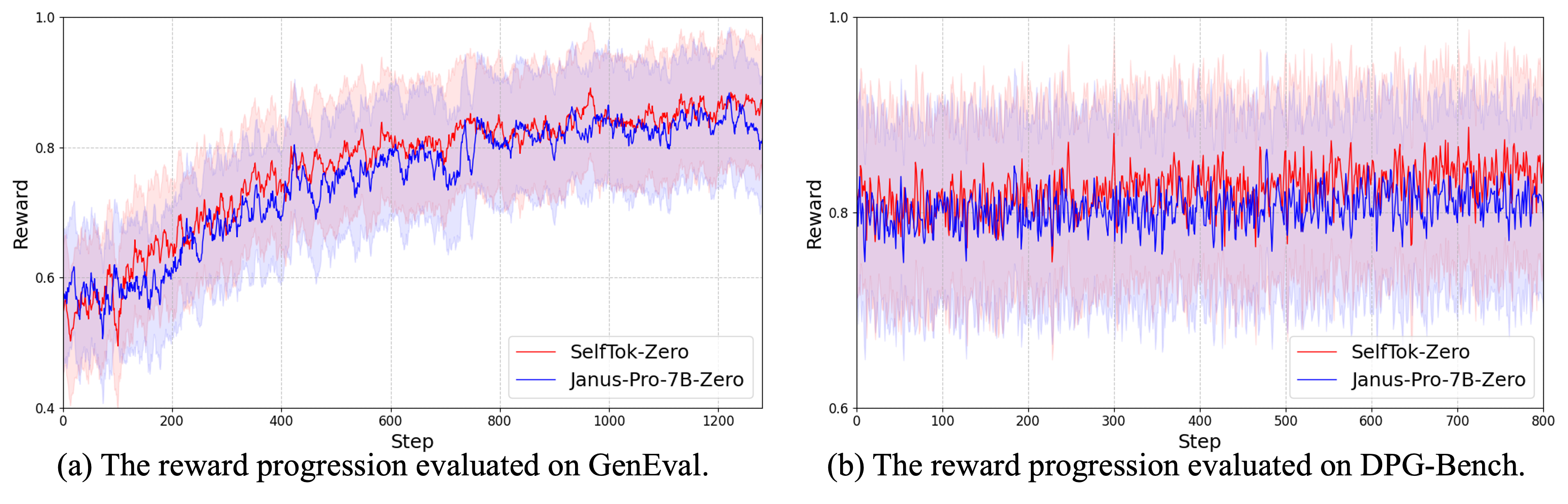
Figure 16: Comparison of reward progression over steps for Selftok (Selftok-Zero) and spatial tokens (Janus-Pro-7B-Zero) on GenEval and DPG-Bench.

Selftok is more effective than spatial tokens in visual RL. The results in Table 7 and Table 8 show that Selftok significantly outperforms spatial token-based methods in visual reinforcement learning (e.g., Janus-Pro-7B-Zero +6 vs Selftok-Zero +18 on GenEval). Figure 16 illustrates the reward score changes during visual RL evaluation on GenEval and DPG-Bench. It is evident that although Janus-Pro-7B^† (79) outperforms Selftok-SFT (74) before visual RL, Selftok-Zero comes from behind to surpass Janus-Pro-7B-Zero (e.g., +7 on Geneval), thanks to the AR properties of Selftok (see Section 4.1). These results further highlight the significant impact of the image tokenizer design on visual RL.

Program-based reward yields more substantial gains in visual RL. We observe that the improvements on GenEval (program-based reward) are more pronounced than on DPG-Bench (QA-based reward). While Selftok-Zero outperforms Selftok-SFT by +21 in overall score on GenEval (74$\rightarrow$95), the improvement on DPG-Bench is slightly smaller (+3.77, 81.80$\rightarrow$85.57). This suggests that program-based reward—enabled by structured detectors and precise matching—provides stronger and more reliable training signals during reinforcement learning, especially for attributes like object counting, color, and spatial layout.

Type	Method	Single Obj.	Two Obj.	Counting	Colors	Position	Color Attr.	Overall
Diffusion Only	PixArt-$\alpha$ [10]	98	50	44	80	8	7	48
	SDXL [88]	98	74	39	85	15	23	55
	FLUX.1-dev [57]	98	79	73	77	22	45	66
	DALL-E 3 [100]	96	87	47	83	43	45	67
	SD3-Medium [24]	99	94	72	89	33	60	74
	CogView4-6B [3]	99	86	66	79	48	58	73
	HiDream-I1 [41]	100	98	79	91	60	72	83
Hybrid Model	SEED-X [29]	97	58	26	80	19	14	49
	Transfusion [133]	-	-	-	-	-	-	63
	D-DiT [64]	97	80	54	76	32	50	65
	Show-o [124]	98	80	66	84	31	50	68
	GPT-4o${\ddagger}$ [81]	99	92	85	91	75	66	85
Pure dAR	Emu3-Gen [116]	98	71	34	81	17	21	54
	TokenFlow-XL [89]	95	60	41	81	16	24	55
	ILLUME+ [49]	99	88	62	84	42	53	72
	Infinity [38]	-	85	-	-	49	57	73
	Janus-Pro-7B [13]	99	89	59	90	79	66	80
	Janus-Pro-7B$\dagger$	98	88	58	88	76	65	79
	Janus-Pro-7B-Zero	98+0	95+7	58+0	89+1	90+14	81+16	85+6
	Selftok-Pre	99	57	58	81	22	43	60
	Sefltok-Pre-Zero	99 +0	94 +37	58 +0	89 +8	89 +67	73 +30	84 +24
	Selftok-SFT	100	79	66	91	45	62	74
	Selftok-Zero	100+0	98+19	90+24	97+6	98+53	90+28	95+21

Table 7: Evaluation of text-to-image generation ability on GenEval benchmark. Janus-Pro-7B$\dagger$ represents the result of our evaluation. Janus-Pro-7B-Zero represents a model that has undergone the same visual RL process as Selftok-Pre-Zero and Selftok-Zero.

Type	Method	Global	Entity	Attribute	Relation	Other	Overall
Diffusion Only	PixArt-$\alpha$ [10]	74.97	79.32	78.60	82.57	76.96	71.11
	SDXL [88]	83.27	82.43	80.91	86.76	80.41	74.65
	DALL-E 3 [100]	90.97	89.61	88.39	90.58	89.83	83.50
	SD3-Medium [24]	87.90	91.01	88.83	80.70	88.68	84.08
	FLUX.1-dev [57]	85.80	86.79	89.98	90.04	89.90	83.79
	CogView4-6B [3]	83.85	90.35	91.17	91.14	87.29	85.13
	HiDream-I1 [41]	76.44	90.22	89.48	93.74	91.83	85.89
Hybrid Model	Show-o [124]	-	-	-	-	-	67.48
Pure dAR	Emu3-Gen [116]	85.21	86.68	86.84	90.22	83.15	80.60
	Janus [121]	82.33	87.38	87.70	85.46	86.41	79.68
	Infinity [38]	93.11	-	-	90.76	-	83.46
	Janus-Pro-7B [13]	86.90	88.90	89.40	89.32	89.48	84.19
	Janus-Pro-7B$\dagger$	83.59	89.74	87.51	92.94	81.20	83.48
	Janus-Pro-7B-Zero	84.50+0.91	90.13+0.39	87.29-0.22	93.44+0.50	82.40+1.20	84.49+1.01
	Selftok-Pre	87.41	87.09	88.08	87.89	87.42	80.37
	Selftok-SFT	82.07	88.15	87.69	93.68	80.40	81.80
	Selftok-Zero	83.59+1.52	91.78+3.63	89.04+1.35	95.26+1.58	82.80+2.40	85.57+3.77

Table 8: Performances on DPG-Bench. The methods in this table are all generation-specific models except Show-o, Janus-Pro, and Selftok.

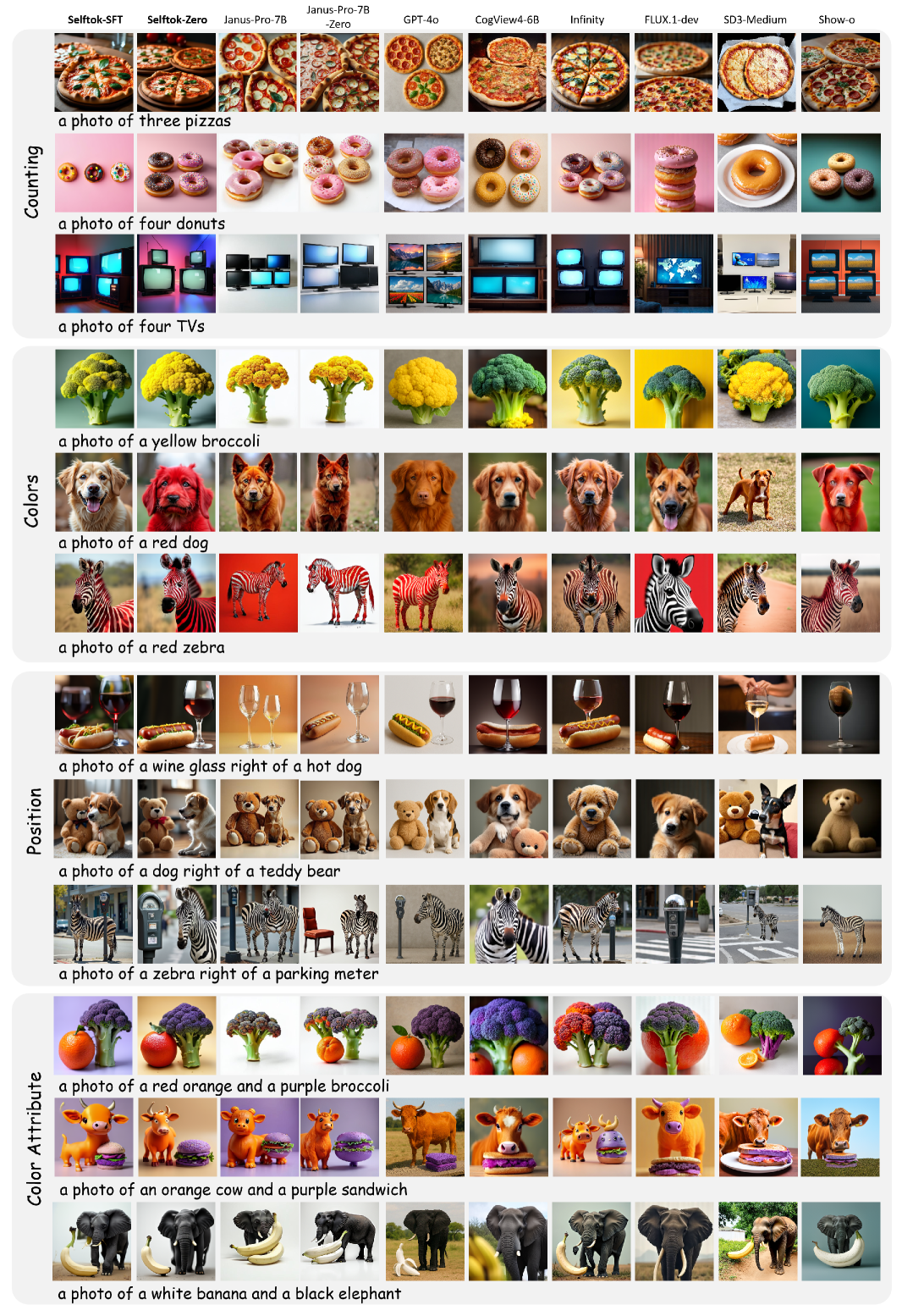
Figure 17: Qualitative experimental results of Selftok-based visual RL. Compared to existing text-to-image generation models, the images generated by Selftok demonstrate better alignment with the given prompts.

5 Conclusion, Limitations, and Ongoing Work

In this paper, we propose Selftok, a non-spatial 1D visual tokenizer that encodes images into discrete tokens conforming to an autoregressive (AR) structure. We argue that this token structure is crucial for multimodal training: 1) AR visual tokens are inherently compatible with language tokens and large language models (LLMs), which are autoregressive by design; and 2) AR visual tokens enable optimal policy improvement for effective visual reinforcement learning (RL). We demonstrate that Selftok’s AR structure emerges from the reverse diffusion process. To the best of our knowledge, this is the first work to unify diffusion and autoregression within a single LLM framework, without introducing additional architectures or training objectives.

The primary limitation does not lie in Selftok itself, but rather in the significantly slower token generation speed of LLMs compared to diffusion models. For instance, when using 512 tokens per frame, generating a one-minute video clip at 24 fps would require generating $512\times 24\times 60=737,280$ tokens—posing a substantial throughput challenge. Fortunately, we are optimistic that this issue will be mitigated by introducing spatial-temporal compression, in conjunction with the rapid progress in real-time massive token generation within the LLM community [32]. Another limitation of this work stems from the restricted model scale. Due to limited capacity, we have not yet demonstrated Selftok’s ability to transfer visual knowledge to language and realize multimodal emergent capabilities. If resources permit, we plan to investigate the scaling laws of multimodal training with Selftok, aiming to validate its potential for cross-modal synergy. Next, we highlight our two ongoing works for Selftok:

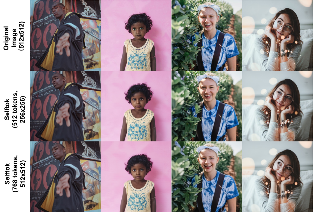
Figure 18: Qualitative results of $512\times 512$ resolutions.

Multi-resolution Selftok. The current resolution of Selftok is limited to $256\times 256$, which constrains the quality of visual generation. Our design follows an incremental principle: higher-resolution images are supported by increasing the number of tokens, while reusing the tokens extracted from their lower-resolution counterparts. This enables efficient scalability, allowing higher-resolution data to leverage a dAR model pre-trained on lower-resolution inputs. This approach is particularly appealing, as it parallels the practice in LLM training, where longer document training benefits from prior training on shorter texts. Figure 18 presents our preliminary results, which will be included in the next release of Selftok.

Physics-aware Post-training Inspired by the impressive performance gains of visual RL by using the program-based reward, our next step is to incorporate physical laws into Selftok-based video generation. For example, we can track the trajectories of moving objects and evaluate whether they conform to fundamental motion principles. This direction has great potential in addressing the ever-lasting criticisms that large visual models struggle to learn a true world model [135, 54]. In our recent work, we demonstrated that Selftok can achieve near-perfect object motion generation in a toy visual environment [65].

6 Contributions and Acknowledgments

Core Contributors
Bohan Wang
Zhongqi Yue
Fengda Zhang
Shuo Chen
Li’an Bi
Junzhe Zhang
Xue Song
Kennard Yanting Chan
Jiachun Pan
Weijia Wu
Mingze Zhou
Wang Lin
Kaihang Pan
Saining Zhang
Liyu Jia
Wentao Hu

Tech Lead
Hanwang Zhang

Project Lead
Wei Zhao

Contributors
Dongze Lian
Zhaozheng Chen
Wenzheng Xie
Yiming Huang
Yutong Hu
Zeyi Huang
Yuanlin Chen
Shaokang Ma
Mengchao Bai
Wenhong Gong
Lin Qi
Lifei Zhu
Tianjiao Guo

Appendix

A. VLM Training Data and Evaluation Details

A.1 Training Data

Cross-Modality Pretrain. Our training data is comprised of both our in-house datasets and publicly available resources. These include datasets such as COYO [7], DataComp [27], and specific subsets of LAION-5B [94]. To ensure the high quality of the training data, we applied a series of rigorous filtering steps, including image resolution, NSFW, aesthetics, watermarking, etc. Together with our in-house text datasets, this results in a final high-quality dataset of 530 million image-text pairs and text sequences. A detailed breakdown of the dataset composition is provided in Figure 19. Along with the original captions available in existing datasets, we perform multi-level captioning [60] to capture various levels of information from the images. The multi-level captioning ranges from basic information to more complex elements, covering a spectrum from “subject > surrounding environment > subject action > visual language > camera language > world knowledge”. We use the publicly available QwenVL [114] and MiniCPM [45] for multi-captioning (Example prompts used for multi-captioning are listed as follows). We perform training on 48 nodes with 384 Huawei Ascend 910B2 units. The global batch size is set to 7680, and the learning rate is set to 1e-4, with cosine decay to 1e-5. The total training steps are 200k iterations. We use the AdamW optimizer, with $\beta_{1}=0.9,\beta_{2}=0.95$. During training, one level of caption is randomly selected.

• Level 0: “Summarize the contents of this image in no more than 5 words."

• Level 1: “Provide a concise caption (up to 10 words) that identifies the main subject of the image.”

• Level 2: “Create a short caption (up to 30 words) that describes the main subject of the image and includes a brief mention of its surrounding environment.”

• Level 3: “Generate a caption (up to 60 words) that describes the main subject, the surrounding environment. If the image is a photograph, include elements of visual language.”

• Level 4: “Create a medium-length caption that describes the main subject, its actions, the surrounding environment. If the image is a photograph, includes elements of visual language and camera language. Keep the caption around 50-100 words.”

• Level 5: “Create a caption that describes the main subject of the image, including its actions, the surrounding environment (from three aspects: foreground, mid-range, background), and any relevant world knowledge or named entities. If the image is a photograph, incorporate aspects of the image’s visual style (e.g., lighting, color tone, composition) and camera language (e.g., lens type, depth of field, angle) to enrich the description. Write the caption in fluent, natural language, and keep it around 150-200 words. Emphasize an engaging, informative tone that captures the essence of the scene. Consider any contextual clues from the setting to provide a well-rounded and insightful caption.”

Supervised Fine-Tuning. During this stage, we incorporate a variety of tasks for cross task training, outlined as follows:

(1) Text-to-Image Generation: We curated tens of thousands of in-house image-text pairs for further improving the image-text alignment in the QT phase. In the training stage, the image resolution is set to 256 $\times$ 256. We perform training on one node with 8 Huawei Ascend 910B2 units. The global batch size is set to 32. There are 252,202 samples used in fine-tuning, constructed from our in-house image generation model. The short edges of all images were resized to 256 and then center-cropped to feed into the Selftok tokenizer. The learning rate is set to 1e-5. During inference, the logit adjustment scale is set to $10$ and the entropy threshold is $2.0$.

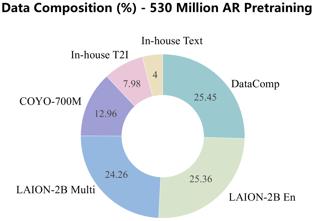
Figure 19: The composition of 530 million AR pretraining data.

(2) Image Editing: The training data for image editing involves our in-house datasets as well as open-source ones, totaling 1,487,148 samples. These public datasets consist of Paint by InPaint Edit (PIPE) [118], UltraEdit [132], and OmniEdit [120], which are manually filtered to guarantee the quality, considering both the fidelity towards source images and the alignment between the instructions and corresponding image pairs. Furthermore, we curated around two thousand in-house editing samples to further enhance the editing performance in the QT phase. The editing categories of our training data cover addition, removal, replacement, change attribution, and style transfer. In the training stage of image editing, the image resolution is set to 256 $\times$ 256. We perform training on two nodes with 8 Huawei Ascend 910B2 units each. The global batch size is set to 128. The large edges of all images are resized to 256, and then the small edges are white-padded to 256 before being fed into the Selftok tokenizer. The learning rate is set to 1e-5. During inference, the logit adjustment scale is set to $7.5$ and the entropy threshold is $2.0$.

Dataset	Introduction
VQAv2 [34]	VQAv2, the updated version of the Visual Question Answering (VQA) dataset, consists of open-ended questions tied to images. To answer these questions, models must have an understanding of visual content, language, and general world knowledge. We transform the dataset into a dialogue format with the instruction: ’Answer the question using a single word or phrase.’
OKVQA [74]	This dataset contains more than 14K questions that necessitate external knowledge for answering, with a focus on knowledge-driven visual question answering.
A-OKVQA [95]	An enhanced version of OKVQA [74], this dataset includes 25K questions that demand a wide range of commonsense and general knowledge for accurate answers.
IconQA [70]	This dataset contains 107K questions divided into three sub-tasks, concentrating on abstract diagram interpretation and in-depth visual reasoning.
GQA [51]	GQA is a comprehensive dataset comprising over 110K images and 22 million questions, designed to pair images with balanced question-answer sets for visual reasoning tasks.
OCR-VQA [76]	The OCR-VQA dataset is a dataset designed for visual question answering that combines optical character recognition (OCR), which contains 207,572 images of book covers and more than 1 million question-answer pairs about these images.
OneVision-Single Image [58]	The LLaVA-OneVision dataset is a high-quality collection comprising 3.2 million images and over 7 million image-question pairs, spanning five major categories: General QA, General OCR, Document/Chart/Screen, Math Reasoning, and Language.
TextVQA [101]	The TextVQA dataset is a benchmark designed to advance VQA systems that require reading and reasoning about text within images. The training set contains 34,602 questions based on 21,953 images from OpenImages training set.
PixMo [18]	The PixMo dataset is a comprehensive collection designed to train the Molmo [18] family of models, among which we use the PixMo-AskModelAnything and PixMo-CapQA subsets. AskModelAnything contains 162k human-authored question-answer pairs across 73k images, enabling models to respond to diverse image-related queries. CapQA features 214k synthetic question-answer pairs derived from 165k dense image captions.
VizWiz [37]	VizWiz originates from real-world scenarios where blind users capture images using mobile phones and pose spoken questions about them. It contains 8k images to evaluate model’s zero-shot generalization on visual questions.

Table 9: Introduction of datasets used in Selftok’s Vision Language Comprehension SFT. The formatting prompts outlined in [66] are used for processing non-dialogue datasets. Note that only the training set is used for training.

(3) Vision-Language Comprehension: During the SFT stage, we used a variety of publicly available training data, as shown in Table 9. Due to the significant differences in data volume across different datasets, we applied a proportional adjustment to the data sizes and then performed joint training. In the training phase of vision-language comprehension, the image resolution is set to 256 $\times$ 256. We train on four nodes, each equipped with 8 Huawei Ascend 910B2 units, and the global batch size is set to 128. The learning rate, similar to other SFT tasks, is set to 1e-5. During inference, we standardize the format by using the instruction: ’Answer the question using a single word or phrase’.

A.2 Inference Process

Algorithm 1 Adaptive Logit Adjustment Inference

Input model $\mathcal{M}$; conditional input $\mathbf{c}$; unconditional input $\mathbf{u}$;

initial generated tokens $\mathbf{r}$; entropy threshold $\tau$; adjustment scale $\gamma$

1:$\mathbf{r}\leftarrow\emptyset$

2:for $i=1,\dots,N$ do $\triangleright$ Iterate over token indices

3:  $\mathbf{logit}_{c}\leftarrow\mathcal{M}(\mathbf{c},\mathbf{r})$ $\triangleright$ Compute logits for conditional input

4:  $\mathbf{logit}_{u}\leftarrow\mathcal{M}(\mathbf{u},\mathbf{r})$ $\triangleright$ Compute logits for unconditional input

5:  if $\text{entropy}(\mathbf{logit}_{c})>\tau$ then $\triangleright$ Check if entropy exceeds threshold

6:    $\mathbf{logit}_{\text{adjusted}}\leftarrow\mathbf{logit}_{c}+(\gamma-1)\cdot(\mathbf{logit}_{c}-\mathbf{logit}_{u})$ $\triangleright$ Adjust logits based on entropy

7:  else

8:    $\mathbf{logit}_{\text{adjusted}}\leftarrow\mathbf{logit}_{c}$ $\triangleright$ No adjustment applied

9:  end if

10:  $\mathbf{logit}_{\text{top-k}}\leftarrow\text{top-k}(\mathbf{logit}_{\text{adjusted}})$ $\triangleright$ Apply top-k sampling

11:  $\mathbf{p}_{\text{top-k}}\leftarrow\text{softmax}(\mathbf{logit}_{\text{top-k}})$ $\triangleright$ Normalize top-k logits to probabilities

12:  $t_{\text{next}}\leftarrow\text{sample}(\mathbf{p}_{\text{top-k}})$ $\triangleright$ Sample next token

13:  $\mathbf{r}\leftarrow\mathbf{r}\cup t_{\text{next}}$ $\triangleright$ Append sampled token

14:end for

Output generated tokens $\mathbf{r}$

Figure 20: Comparison of inference entropy at different iters.

We propose an adaptive strategy for logit adjustment during inference, with the pseudo code presented in Algorithm 1. Previous methods [9, 116] have referred to this logit adjustment as classifier-free guidance (CFG) . However, we note that the logit adjustment in AR models cannot be derived from Bayesian principles as done in diffusion-based approaches ([43, 20]). Therefore, we prefer to refer to this process as logit adjustment, rather than CFG.

The core idea of our new approach is that logit adjustment is unnecessary when the token entropy is low. Low entropy indicates that the model has high confidence in its prediction for the current token, and further adjustment is not required. During the pretraining process, we also monitor entropy evolution. The Figure 20 illustrates the change in token entropy across different timesteps during training. Key observations include: (1) as training progresses, the overall entropy decreases, suggesting that the model becomes more confident; and (2) as the number of generated tokens increases, the entropy for subsequent tokens decreases, indicating that the model is more certain in predicting future tokens.

It is important to highlight why language models in the AR paradigm do not require logit adjustment, whereas Selftok models do. While we believe that visual tokens in Selftok are similar to language tokens, insufficient training of visual tokens leads to high entropy at certain timesteps. Consequently, logit adjustment is needed to improve generation quality. However, with large-scale video token pretraining, Selftok models will overcome this issue, and similar to language models, logit adjustment will no longer be necessary during inference.

A.3 Evaluation Details

Image Editing: To quantitatively evaluate the editing capability, we employ the widely used PIE-Bench dataset [53] containing 700 testing samples with 10 types of editing: (0) random editing; (1) change object; (2) add object; (3) delete object; (4) change object content; (5) change object pose; (6) change object color; (7) change object material; (8) change image background; (9) change image style. For each editing type, source images are equally divided into artificial and natural ones, where each kind of image is further equally distributed to four scenes, i.e., animal, human, indoor, and outdoor. For metrics, we follow previous works [53, 79] in the perspective of both fidelity and editability using annotated foreground masks. Firstly, fidelity measures the similarity between source and edited images via the following metrics. Structure Distance ($\times 10^{3}$) calculates self-similarity matrices of DINO-ViT features and then applies cosine similarity between matrices of source and edited images. Apart from structure evaluation, PSNR, LPIPS ($\times 10^{3}$), MSE ($\times 10^{4}$), and SSIM ($\times 10^{2}$) are utilized to assess background preservation with annotated masks. Secondly, editability evaluates the alignment between the target image prompts and edited images. Specifically, the CLIP score ($\times 10^{2}$) is computed considering both the whole images and edited regions in the images. All metrics are compared at the resolution of $512\times 512$.

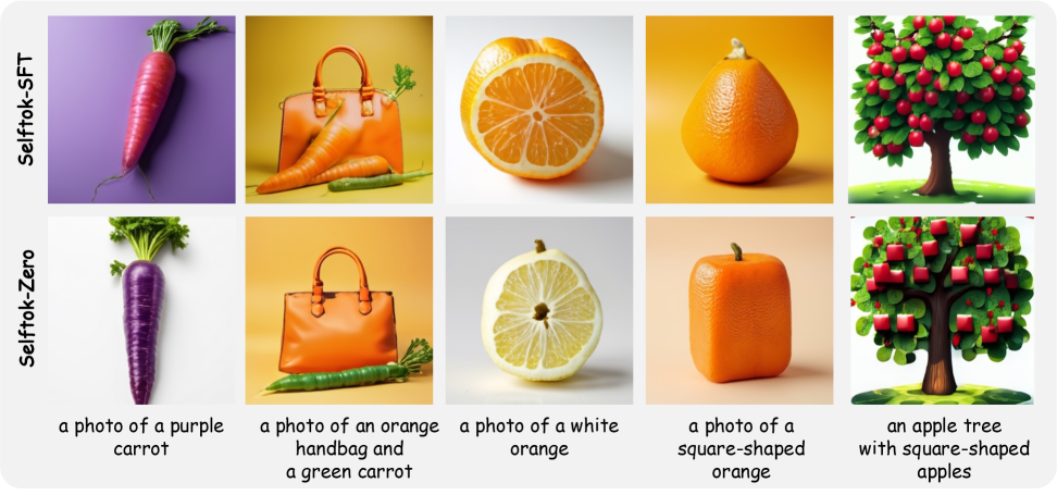
Figure 21: More examples of failures in the Selftok-SFT model due to distributional biases in the training data during vision-language supervised training.

B. Selftok-based Visual RL

Hallucination in Text-to-Image Generation. As discussed in the main text, one of the challenges in text-to-image generation is the “hallucination” issue, where a Vision-Language Model (VLM) tends to generate images that closely follow the training data distribution rather than genuinely reason about the text prompt. This can lead to the model failing to generate certain objects or scenes that are less common or not well-represented in the training set.

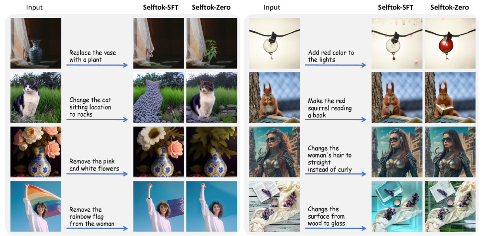
Figure 22: Qualitative experimental results of Selftok-based visual RL on image editing. Compared to the Selftok-SFT, the images generated by Selftok-Zero demonstrate better alignment with the given instructions and better visual fidelity.

In Figure 21, we provide examples where the Selftok-SFT model fails to generate certain objects due to the rarity of these combinations in the training data. However, after applying visual RL (Selftok-Zero), the model is able to generate these previously missing combinations, showing a significant improvement in handling rare or complex prompts. The ability of Selftok-Zero to generate these images after the visual RL phase highlights how reinforcement learning can effectively overcome the hallucination problem, improving the model’s generalization and reasoning capabilities beyond the initial supervised training.

Visual RL for Image Editing. To further unlock the potential of our model, we also incorporate Visual RL into the image editing task, where we utilize a Vision-Language Model (VLM)—specifically, InternVL2.5-78B [14]—as the reward model. This model evaluates whether the generated image strictly follows the instructions and accurately modifies the source image. Inspired by the work of [35, 28], we ask the reward model to return a score between 0 and 5, with 5 indicating the highest level of adherence to the instructions. In a few hundred steps, our Selftok-Zero model shows a significant improvement over the Selftok-SFT model. As shown in Figure 22, our model can correctly correspond to the instructions and generate appropriate edited images.

Unlike text-to-image generation, image editing involves more nuanced transformations, making it significantly more challenging to evaluate automatically. The complexity arises from the need to assess both the fidelity of the edits to the original image and the accuracy of the applied changes according to the given instructions. Therefore, to provide a more general and accurate reward for image editing tasks, we plan to explore more sophisticated reward models that can handle the intricacies of image modification. Additionally, we aim to develop refined evaluation principles that can better capture the subtlety and precision required in image editing. This will be a key focus in our future work, where we hope to improve the reliability of automated assessments and provide more meaningful feedback.

References

- [1] Niket Agarwal, Arslan Ali, Maciej Bala, Yogesh Balaji, Erik Barker, Tiffany Cai, Prithvijit Chattopadhyay, Yongxin Chen, Yin Cui, Yifan Ding, et al. Cosmos world foundation model platform for physical ai. arXiv preprint arXiv:2501.03575, 2025.
- [2] Meta AI. Llama: Open and efficient foundation language models. https://www.llama.com/. Accessed: 2025-04-07.
- [3] Zhipu AI. Cogview4: Next-generation image creation. https://cogview4.net/, 2025.
- [4] Roman Bachmann, Jesse Allardice, David Mizrahi, Enrico Fini, Oğuzhan Fatih Kar, Elmira Amirloo, Alaaeldin El-Nouby, Amir Zamir, and Afshin Dehghan. Flextok: Resampling images into 1d token sequences of flexible length. arXiv preprint arXiv:2502.13967, 2025.
- [5] Jinze Bai, Shuai Bai, Shusheng Yang, Shijie Wang, Sinan Tan, Peng Wang, Junyang Lin, Chang Zhou, and Jingren Zhou. Qwen-vl: A versatile vision-language model for understanding, localization, text reading, and beyond. arXiv preprint arXiv:2308.12966, 2023.
- [6] Tim Brooks, Aleksander Holynski, and Alexei A Efros. Instructpix2pix: Learning to follow image editing instructions. In Proceedings of the IEEE/CVF conference on computer vision and pattern recognition, pages 18392–18402, 2023.
- [7] Minwoo Byeon, Beomhee Park, Haecheon Kim, Sungjun Lee, Woonhyuk Baek, and Saehoon Kim. Coyo-700m: Image-text pair dataset. https://github.com/kakaobrain/coyo-dataset, 2022.
- [8] Mingdeng Cao, Xintao Wang, Zhongang Qi, Ying Shan, Xiaohu Qie, and Yinqiang Zheng. Masactrl: Tuning-free mutual self-attention control for consistent image synthesis and editing. In Proceedings of the IEEE/CVF international conference on computer vision, pages 22560–22570, 2023.
- [9] Huiwen Chang, Han Zhang, Jarred Barber, AJ Maschinot, Jose Lezama, Lu Jiang, Ming-Hsuan Yang, Kevin Murphy, William T Freeman, Michael Rubinstein, et al. Muse: Text-to-image generation via masked generative transformers. arXiv preprint arXiv:2301.00704, 2023.
- [10] Junsong Chen, Jincheng Yu, Chongjian Ge, Lewei Yao, Enze Xie, Yue Wu, Zhongdao Wang, James Kwok, Ping Luo, Huchuan Lu, et al. Pixart-: Fast training of diffusion transformer for photorealistic text-to-image synthesis. arXiv preprint arXiv:2310.00426, 2023.
- [11] Kai Chen, Jiaqi Wang, Jiangmiao Pang, Yuhang Cao, Yu Xiong, Xiaoxiao Li, Shuyang Sun, Wansen Feng, Ziwei Liu, Jiarui Xu, et al. Mmdetection: Open mmlab detection toolbox and benchmark. arXiv preprint arXiv:1906.07155, 2019.
- [12] Liang Chen, Zekun Wang, Shuhuai Ren, Lei Li, Haozhe Zhao, Yunshui Li, Zefan Cai, Hongcheng Guo, Lei Zhang, Yizhe Xiong, et al. Next token prediction towards multimodal intelligence: A comprehensive survey. arXiv preprint arXiv:2412.18619, 2024.
- [13] Xiaokang Chen, Zhiyu Wu, Xingchao Liu, Zizheng Pan, Wen Liu, Zhenda Xie, Xingkai Yu, and Chong Ruan. Janus-pro: Unified multimodal understanding and generation with data and model scaling. arXiv preprint arXiv:2501.17811, 2025.
- [14] Zhe Chen, Weiyun Wang, Yue Cao, Yangzhou Liu, Zhangwei Gao, Erfei Cui, Jinguo Zhu, Shenglong Ye, Hao Tian, Zhaoyang Liu, et al. Expanding performance boundaries of open-source multimodal models with model, data, and test-time scaling, 2024.
- [15] Zhe Chen, Jiannan Wu, Wenhai Wang, Weijie Su, Guo Chen, Sen Xing, Muyan Zhong, Qinglong Zhang, Xizhou Zhu, Lewei Lu, et al. Internvl: Scaling up vision foundation models and aligning for generic visual-linguistic tasks. In Proceedings of the IEEE/CVF conference on computer vision and pattern recognition, pages 24185–24198, 2024.
- [16] Jaemin Cho, Yushi Hu, Roopal Garg, Peter Anderson, Ranjay Krishna, Jason Baldridge, Mohit Bansal, Jordi Pont-Tuset, and Su Wang. Davidsonian scene graph: Improving reliability in fine-grained evaluation for text-to-image generation. arXiv preprint arXiv:2310.18235, 2023.
- [17] Wenliang Dai, Junnan Li, DONGXU LI, Anthony Tiong, Junqi Zhao, Weisheng Wang, Boyang Li, Pascale N Fung, and Steven Hoi. Instructblip: Towards general-purpose vision-language models with instruction tuning. Advances in Neural Information Processing Systems, 36:49250–49267, 2023.
- [18] Matt Deitke, Christopher Clark, Sangho Lee, Rohun Tripathi, Yue Yang, Jae Sung Park, Mohammadreza Salehi, Niklas Muennighoff, Kyle Lo, Luca Soldaini, et al. Molmo and pixmo: Open weights and open data for state-of-the-art multimodal models. arXiv preprint arXiv:2409.17146, 2024.
- [19] Jia Deng, Wei Dong, Richard Socher, Li-Jia Li, Kai Li, and Li Fei-Fei. Imagenet: A large-scale hierarchical image database. In Proceedings of the IEEE Conference on Computer Vision and Pattern Recognition (CVPR), pages 248–255, 2009.
- [20] Prafulla Dhariwal and Alexander Nichol. Diffusion models beat gans on image synthesis. Advances in neural information processing systems, 34:8780–8794, 2021.
- [21] Xiaoyi Dong, Pan Zhang, Yuhang Zang, Yuhang Cao, Bin Wang, Linke Ouyang, Xilin Wei, Songyang Zhang, Haodong Duan, Maosong Cao, Wenwei Zhang, Yining Li, Hang Yan, Yang Gao, Xinyue Zhang, Wei Li, Jingwen Li, Kai Chen, Conghui He, Xingcheng Zhang, Yu Qiao, Dahua Lin, and Jiaqi Wang. Internlm-xcomposer2: Mastering free-form text-image composition and comprehension in vision-language large model. arXiv preprint arXiv:2401.16420, 2024.
- [22] Alexey Dosovitskiy, Lucas Beyer, Alexander Kolesnikov, Dirk Weissenborn, Xiaohua Zhai, Thomas Unterthiner, Mostafa Dehghani, Matthias Minderer, G Heigold, S Gelly, et al. An image is worth 16x16 words: Transformers for image recognition at scale. In International Conference on Learning Representations, 2020.
- [23] Shivam Duggal, Phillip Isola, Antonio Torralba, and William T Freeman. Adaptive length image tokenization via recurrent allocation. In First Workshop on Scalable Optimization for Efficient and Adaptive Foundation Models, 2024.
- [24] Patrick Esser, Sumith Kulal, Andreas Blattmann, Rahim Entezari, Jonas Müller, Harry Saini, Yam Levi, Dominik Lorenz, Axel Sauer, Frederic Boesel, et al. Scaling rectified flow transformers for high-resolution image synthesis. In Forty-first international conference on machine learning, 2024.
- [25] Patrick Esser, Robin Rombach, and Bjorn Ommer. Taming transformers for high-resolution image synthesis. In Proceedings of the IEEE/CVF conference on computer vision and pattern recognition, pages 12873–12883, 2021.
- [26] Tsu-Jui Fu, Wenze Hu, Xianzhi Du, William Yang Wang, Yinfei Yang, and Zhe Gan. Guiding instruction-based image editing via multimodal large language models. arXiv preprint arXiv:2309.17102, 2023.
- [27] Samir Yitzhak Gadre, Gabriel Ilharco, Alex Fang, Jonathan Hayase, Georgios Smyrnis, Thao Nguyen, Ryan Marten, Mitchell Wortsman, Dhruba Ghosh, Jieyu Zhang, Eyal Orgad, Rahim Entezari, Giannis Daras, Sarah Pratt, Vivek Ramanujan, Yonatan Bitton, Kalyani Marathe, Stephen Mussmann, Richard Vencu, Mehdi Cherti, Ranjay Krishna, Pang Wei Koh, Olga Saukh, Alexander Ratner, Shuran Song, Hannaneh Hajishirzi, Ali Farhadi, Romain Beaumont, Sewoong Oh, Alex Dimakis, Jenia Jitsev, Yair Carmon, Vaishaal Shankar, and Ludwig Schmidt. Datacomp: In search of the next generation of multimodal datasets. arXiv preprint arXiv:2304.14108, 2023.
- [28] Yu Gao, Lixue Gong, Qiushan Guo, Xiaoxia Hou, Zhichao Lai, Fanshi Li, Liang Li, Xiaochen Lian, Chao Liao, Liyang Liu, Wei Liu, Yichun Shi, Shiqi Sun, Yu Tian, Zhi Tian, Peng Wang, Rui Wang, Xuanda Wang, Xun Wang, Ye Wang, Guofeng Wu, Jie Wu, Xin Xia, Xuefeng Xiao, Zhonghua Zhai, Xinyu Zhang, Qi Zhang, Yuwei Zhang, Shijia Zhao, Jianchao Yang, and Weilin Huang. Seedream 3.0 technical report, 2025.
- [29] Yuying Ge, Sijie Zhao, Jinguo Zhu, Yixiao Ge, Kun Yi, Lin Song, Chen Li, Xiaohan Ding, and Ying Shan. Seed-x: Multimodal models with unified multi-granularity comprehension and generation. arXiv preprint arXiv:2404.14396, 2024.
- [30] Zigang Geng, Binxin Yang, Tiankai Hang, Chen Li, Shuyang Gu, Ting Zhang, Jianmin Bao, Zheng Zhang, Houqiang Li, Han Hu, et al. Instructdiffusion: A generalist modeling interface for vision tasks. In Proceedings of the IEEE/CVF Conference on computer vision and pattern recognition, pages 12709–12720, 2024.
- [31] Dhruba Ghosh, Hannaneh Hajishirzi, and Ludwig Schmidt. Geneval: An object-focused framework for evaluating text-to-image alignment. Advances in Neural Information Processing Systems, 36:52132–52152, 2023.
- [32] Fabian Gloeckle, Badr Youbi Idrissi, Baptiste Rozière, David Lopez-Paz, and Gabriel Synnaeve. Better & faster large language models via multi-token prediction. arXiv preprint arXiv:2404.19737, 2024.
- [33] Ian Goodfellow, Jean Pouget-Abadie, Mehdi Mirza, Bing Xu, David Warde-Farley, Sherjil Ozair, Aaron Courville, and Yoshua Bengio. Generative adversarial networks. Communications of the ACM, 63(11):139–144, 2020.
- [34] Yash Goyal, Tejas Khot, Douglas Summers-Stay, Dhruv Batra, and Devi Parikh. Making the v in vqa matter: Elevating the role of image understanding in visual question answering. In CVPR, pages 6904–6913, 2017.
- [35] Xin Gu, Ming Li, Libo Zhang, Fan Chen, Longyin Wen, Tiejian Luo, and Sijie Zhu. Multi-reward as condition for instruction-based image editing, 2024.
- [36] Daya Guo, Dejian Yang, Haowei Zhang, Junxiao Song, Ruoyu Zhang, Runxin Xu, Qihao Zhu, Shirong Ma, Peiyi Wang, Xiao Bi, et al. Deepseek-r1: Incentivizing reasoning capability in llms via reinforcement learning. arXiv preprint arXiv:2501.12948, 2025.
- [37] Danna Gurari, Qing Li, Abigale J Stangl, Anhong Guo, Chi Lin, Kristen Grauman, Jiebo Luo, and Jeffrey P Bigham. Vizwiz grand challenge: Answering visual questions from blind people. In Proceedings of the IEEE conference on computer vision and pattern recognition, pages 3608–3617, 2018.
- [38] Jian Han, Jinlai Liu, Yi Jiang, Bin Yan, Yuqi Zhang, Zehuan Yuan, Bingyue Peng, and Xiaobing Liu. Infinity: Scaling bitwise autoregressive modeling for high-resolution image synthesis, 2024.
- [39] Amir Hertz, Ron Mokady, Jay Tenenbaum, Kfir Aberman, Yael Pritch, and Daniel Cohen-Or. Prompt-to-prompt image editing with cross attention control. arXiv preprint arXiv:2208.01626, 2022.
- [40] Martin Heusel, Hubert Ramsauer, Thomas Unterthiner, Bernhard Nessler, and Sepp Hochreiter. Gans trained by a two time-scale update rule converge to a local nash equilibrium. Advances in neural information processing systems, 30, 2017.
- [41] HiDream-ai. Hidream-i1. https://hidreamai.com, 2025.
- [42] Irina Higgins, David Amos, David Pfau, Sebastien Racaniere, Loic Matthey, Danilo Rezende, and Alexander Lerchner. Towards a definition of disentangled representations. arXiv preprint arXiv:1812.02230, 2018.
- [43] Jonathan Ho and Tim Salimans. Classifier-free diffusion guidance. arXiv preprint arXiv:2207.12598, 2022.
- [44] Kyle Hsu, William Dorrell, James Whittington, Jiajun Wu, and Chelsea Finn. Disentanglement via latent quantization. Advances in Neural Information Processing Systems, 36:45463–45488, 2023.
- [45] Shengding Hu, Yuge Tu, Xu Han, Chaoqun He, Ganqu Cui, Xiang Long, Zhi Zheng, Yewei Fang, Yuxiang Huang, Weilin Zhao, et al. Minicpm: Unveiling the potential of small language models with scalable training strategies. arXiv preprint arXiv:2404.06395, 2024.
- [46] Tianyang Hu, Jun Wang, Wenjia Wang, and Zhenguo Li. Understanding square loss in training overparametrized neural network classifiers. Advances in Neural Information Processing Systems, 35:16495–16508, 2022.
- [47] Xiwei Hu, Rui Wang, Yixiao Fang, Bin Fu, Pei Cheng, and Gang Yu. Ella: Equip diffusion models with llm for enhanced semantic alignment, 2024.
- [48] Xiwei Hu, Rui Wang, Yixiao Fang, Bin Fu, Pei Cheng, and Gang Yu. Ella: Equip diffusion models with llm for enhanced semantic alignment. arXiv preprint arXiv:2403.05135, 2024.
- [49] Runhui Huang, Chunwei Wang, Junwei Yang, Guansong Lu, Yunlong Yuan, Jianhua Han, Lu Hou, Wei Zhang, Lanqing Hong, Hengshuang Zhao, and Hang Xu. Illume+: Illuminating unified mllm with dual visual tokenization and diffusion refinement. arXiv preprint arXiv:2504.01934, 2025.
- [50] Wenxuan Huang, Bohan Jia, Zijie Zhai, Shaosheng Cao, Zheyu Ye, Fei Zhao, Yao Hu, and Shaohui Lin. Vision-r1: Incentivizing reasoning capability in multimodal large language models. arXiv preprint arXiv:2503.06749, 2025.
- [51] Drew A Hudson and Christopher D Manning. Gqa: A new dataset for real-world visual reasoning and compositional question answering. In CVPR, pages 6700–6709, 2019.
- [52] Aaron Hurst, Adam Lerer, Adam P Goucher, Adam Perelman, Aditya Ramesh, Aidan Clark, AJ Ostrow, Akila Welihinda, Alan Hayes, Alec Radford, et al. Gpt-4o system card. arXiv preprint arXiv:2410.21276, 2024.
- [53] Xuan Ju, Ailing Zeng, Yuxuan Bian, Shaoteng Liu, and Qiang Xu. Direct inversion: Boosting diffusion-based editing with 3 lines of code. arXiv preprint arXiv:2310.01506, 2023.
- [54] Bingyi Kang, Yang Yue, Rui Lu, Zhijie Lin, Yang Zhao, Kaixin Wang, Gao Huang, and Jiashi Feng. How far is video generation from world model: A physical law perspective. arXiv preprint arXiv:2411.02385, 2024.
- [55] Tero Karras, Samuli Laine, and Timo Aila. A style-based generator architecture for generative adversarial networks. In Proceedings of the IEEE/CVF conference on computer vision and pattern recognition, pages 4401–4410, 2019.
- [56] Dan Kondratyuk, Lijun Yu, Xiuye Gu, José Lezama, Jonathan Huang, Grant Schindler, Rachel Hornung, Vighnesh Birodkar, Jimmy Yan, Ming-Chang Chiu, et al. Videopoet: A large language model for zero-shot video generation. arXiv preprint arXiv:2312.14125, 2023.
- [57] Black Forest Labs. Flux. https://github.com/black-forest-labs/flux, 2024.
- [58] Bo Li, Yuanhan Zhang, Dong Guo, Renrui Zhang, Feng Li, Hao Zhang, Kaichen Zhang, Peiyuan Zhang, Yanwei Li, Ziwei Liu, et al. Llava-onevision: Easy visual task transfer. arXiv preprint arXiv:2408.03326, 2024.
- [59] Chenliang Li, Haiyang Xu, Junfeng Tian, Wei Wang, Ming Yan, Bin Bi, Jiabo Ye, Hehong Chen, Guohai Xu, Zheng Cao, et al. mplug: Effective and efficient vision-language learning by cross-modal skip-connections. arXiv preprint arXiv:2205.12005, 2022.
- [60] Daiqing Li, Aleks Kamko, Ehsan Akhgari, Ali Sabet, Linmiao Xu, and Suhail Doshi. Playground v2. 5: Three insights towards enhancing aesthetic quality in text-to-image generation. arXiv preprint arXiv:2402.17245, 2024.
- [61] Li Li, Jiashu Qu, Yuxiao Zhou, Yuehan Qin, Tiankai Yang, and Yue Zhao. Treble counterfactual vlms: A causal approach to hallucination. arXiv preprint arXiv:2503.06169, 2025.
- [62] Tianhong Li, Yonglong Tian, He Li, Mingyang Deng, and Kaiming He. Autoregressive image generation without vector quantization. Advances in Neural Information Processing Systems, 37:56424–56445, 2024.
- [63] Xiang Li, Kai Qiu, Hao Chen, Jason Kuen, Jiuxiang Gu, Bhiksha Raj, and Zhe Lin. Imagefolder: Autoregressive image generation with folded tokens. arXiv preprint arXiv:2410.01756, 2024.
- [64] Zijie Li, Henry Li, Yichun Shi, Amir Barati Farimani, Yuval Kluger, Linjie Yang, and Peng Wang. Dual diffusion for unified image generation and understanding. arXiv preprint arXiv:2501.00289, 2024.
- [65] Wang Lin, Liyu Jia, Wentao Hu, Kaihang Pan, Zhongqi Yue, Wei Zhao, Jingyuan Chen, Fei Wu, and Hanwang Zhang. Reasoning physical video generation with diffusion timestep tokens via reinforcement learning. In submission, 2025.
- [66] Haotian Liu, Chunyuan Li, Yuheng Li, and Yong Jae Lee. Improved baselines with visual instruction tuning. In Proceedings of the IEEE/CVF Conference on Computer Vision and Pattern Recognition, pages 26296–26306, 2024.
- [67] Hao Liu, Wilson Yan, Matei Zaharia, and Pieter Abbeel. World model on million-length video and language with blockwise ringattention. arXiv preprint arXiv:2402.08268, 2024.
- [68] Xingchao Liu, Chengyue Gong, et al. Flow straight and fast: Learning to generate and transfer data with rectified flow. In The Eleventh International Conference on Learning Representations, 2023.
- [69] Francesco Locatello, Stefan Bauer, Mario Lucic, Gunnar Raetsch, Sylvain Gelly, Bernhard Schölkopf, and Olivier Bachem. Challenging common assumptions in the unsupervised learning of disentangled representations. In international conference on machine learning, pages 4114–4124. PMLR, 2019.
- [70] Pan Lu, Liang Qiu, Jiaqi Chen, Tony Xia, Yizhou Zhao, Wei Zhang, Zhou Yu, Xiaodan Liang, and Song-Chun Zhu. Iconqa: A new benchmark for abstract diagram understanding and visual language reasoning. arXiv preprint arXiv:2110.13214, 2021.
- [71] Rui Lu, Runzhe Wang, Kaifeng Lyu, Xitai Jiang, Gao Huang, and Mengdi Wang. Towards understanding text hallucination of diffusion models via local generation bias. arXiv preprint arXiv:2503.03595, 2025.
- [72] Zhuoyan Luo, Fengyuan Shi, Yixiao Ge, Yujiu Yang, Limin Wang, and Ying Shan. Open-magvit2: An open-source project toward democratizing auto-regressive visual generation. arXiv preprint arXiv:2409.04410, 2024.
- [73] Yiyang Ma, Xingchao Liu, Xiaokang Chen, Wen Liu, Chengyue Wu, Zhiyu Wu, Zizheng Pan, Zhenda Xie, Haowei Zhang, Liang Zhao, et al. Janusflow: Harmonizing autoregression and rectified flow for unified multimodal understanding and generation. arXiv preprint arXiv:2411.07975, 2024.
- [74] Kenneth Marino, Mohammad Rastegari, Ali Farhadi, and Roozbeh Mottaghi. Ok-vqa: A visual question answering benchmark requiring external knowledge. In CVPR, pages 3195–3204, 2019.
- [75] Edan Meyer, Adam White, and Marlos C Machado. Harnessing discrete representations for continual reinforcement learning. arXiv preprint arXiv:2312.01203, 2023.
- [76] Anand Mishra, Shashank Shekhar, Ajeet Kumar Singh, and Anirban Chakraborty. Ocr-vqa: Visual question answering by reading text in images. In ICDAR, pages 947–952. IEEE, 2019.
- [77] Keita Miwa, Kento Sasaki, Hidehisa Arai, Tsubasa Takahashi, and Yu Yamaguchi. One-d-piece: Image tokenizer meets quality-controllable compression. arXiv preprint arXiv:2501.10064, 2025.
- [78] Ron Mokady, Amir Hertz, Kfir Aberman, Yael Pritch, and Daniel Cohen-Or. Null-text inversion for editing real images using guided diffusion models. In Proceedings of the IEEE/CVF conference on computer vision and pattern recognition, pages 6038–6047, 2023.
- [79] Jiteng Mu, Nuno Vasconcelos, and Xiaolong Wang. Editar: Unified conditional generation with autoregressive models. arXiv preprint arXiv:2501.04699, 2025.
- [80] Yulei Niu and Hanwang Zhang. Introspective distillation for robust question answering. Advances in Neural Information Processing Systems, 34:16292–16304, 2021.
- [81] OpenAI. Introducing 4o image generation. https://openai.com/index/introducing-4o-image-generation/, 2025. Accessed: 2025-04-22.
- [82] Jiachun Pan, Xingyu Xie, Hanwang Zhang, and Shuicheng YAN. Vr-sampling: Accelerating flow generative model training with variance reduction sampling. 2024.
- [83] Kaihang Pan, Wang Lin, Zhongqi Yue, Tenglong Ao, Liyu Jia, Wei Zhao, Juncheng Li, Siliang Tang, and Hanwang Zhang. Generative mutimodal pretraining with discrete diffusion timestep tokens. In Proceedings of the IEEE/CVF Conference on Computer Vision and Pattern Recognition, 2025.
- [84] Kaihang Pan, Siliang Tang, Juncheng Li, Zhaoyu Fan, Wei Chow, Shuicheng Yan, Tat-Seng Chua, Yueting Zhuang, and Hanwang Zhang. Auto-encoding morph-tokens for multimodal llm. In Proceedings of the 41st International Conference on Machine Learning, pages 39308–39323, 2024.
- [85] Gaurav Parmar, Krishna Kumar Singh, Richard Zhang, Yijun Li, Jingwan Lu, and Jun-Yan Zhu. Zero-shot image-to-image translation. In ACM SIGGRAPH 2023 conference proceedings, pages 1–11, 2023.
- [86] Judea Pearl. Causality: Models, Reasoning, and Inference. Cambridge University Press, New York, NY, USA, 2nd edition, 2009.
- [87] Yi Peng, Xiaokun Wang, Yichen Wei, Jiangbo Pei, Weijie Qiu, Ai Jian, Yunzhuo Hao, Jiachun Pan, Tianyidan Xie, Li Ge, et al. Skywork r1v: Pioneering multimodal reasoning with chain-of-thought. arXiv preprint arXiv:2504.05599, 2025.
- [88] Dustin Podell, Zion English, Kyle Lacey, Andreas Blattmann, Tim Dockhorn, Jonas Müller, Joe Penna, and Robin Rombach. Sdxl: Improving latent diffusion models for high-resolution image synthesis. arXiv preprint arXiv:2307.01952, 2023.
- [89] Liao Qu, Huichao Zhang, Yiheng Liu, Xu Wang, Yi Jiang, Yiming Gao, Hu Ye, Daniel K Du, Zehuan Yuan, and Xinglong Wu. Tokenflow: Unified image tokenizer for multimodal understanding and generation. arXiv preprint arXiv:2412.03069, 2024.
- [90] Alec Radford, Jong Wook Kim, Chris Hallacy, Aditya Ramesh, Gabriel Goh, Sandhini Agarwal, Girish Sastry, Amanda Askell, Pamela Mishkin, Jack Clark, et al. Learning transferable visual models from natural language supervision. In International conference on machine learning, pages 8748–8763. PmLR, 2021.
- [91] Alec Radford, Karthik Narasimhan, Tim Salimans, and Ilya Sutskever. Improving language understanding by generative pre-training. OpenAI Blog, 1(8), 2018.
- [92] Rafael Rafailov, Archit Sharma, Eric Mitchell, Christopher D Manning, Stefano Ermon, and Chelsea Finn. Direct preference optimization: Your language model is secretly a reward model. Advances in Neural Information Processing Systems, 36:53728–53741, 2023.
- [93] Kyle Sargent, Kyle Hsu, Justin Johnson, Li Fei-Fei, and Jiajun Wu. Flow to the mode: Mode-seeking diffusion autoencoders for state-of-the-art image tokenization. arXiv preprint arXiv:2503.11056, 2025.
- [94] Christoph Schuhmann, Romain Beaumont, Richard Vencu, Cade Gordon, Ross Wightman, Mehdi Cherti, Theo Coombes, Aarush Katta, Clayton Mullis, Mitchell Wortsman, et al. Laion-5b: An open large-scale dataset for training next generation image-text models. Advances in neural information processing systems, 35:25278–25294, 2022.
- [95] Dustin Schwenk, Apoorv Khandelwal, Christopher Clark, Kenneth Marino, and Roozbeh Mottaghi. A-okvqa: A benchmark for visual question answering using world knowledge. In ECCV, pages 146–162, 2022.
- [96] Rico Sennrich, Barry Haddow, and Alexandra Birch. Neural machine translation of rare words with subword units. In Proceedings of the 54th Annual Meeting of the Association for Computational Linguistics (Volume 1: Long Papers), pages 1715–1725, Berlin, Germany, 2016. Association for Computational Linguistics.
- [97] Zhihong Shao, Peiyi Wang, Qihao Zhu, Runxin Xu, Junxiao Song, Xiao Bi, Haowei Zhang, Mingchuan Zhang, YK Li, Y Wu, et al. Deepseekmath: Pushing the limits of mathematical reasoning in open language models. arXiv preprint arXiv:2402.03300, 2024.
- [98] Haozhan Shen, Peng Liu, Jingcheng Li, Chunxin Fang, Yibo Ma, Jiajia Liao, Qiaoli Shen, Zilun Zhang, Kangjia Zhao, Qianqian Zhang, et al. Vlm-r1: A stable and generalizable r1-style large vision-language model. arXiv preprint arXiv:2504.07615, 2025.
- [99] Yichun Shi, Peng Wang, and Weilin Huang. Seededit: Align image re-generation to image editing. arXiv preprint arXiv:2411.06686, 2024.
- [100] Zhan Shi, Xu Zhou, Xipeng Qiu, and Xiaodan Zhu. Improving image captioning with better use of captions. arXiv preprint arXiv:2006.11807, 2020.
- [101] Amanpreet Singh, Vivek Natarajan, Meet Shah, Yu Jiang, Xinlei Chen, Dhruv Batra, Devi Parikh, and Marcus Rohrbach. Towards vqa models that can read. In Proceedings of the IEEE/CVF conference on computer vision and pattern recognition, pages 8317–8326, 2019.
- [102] Yang Song, Prafulla Dhariwal, Mark Chen, and Ilya Sutskever. Consistency models. In International Conference on Machine Learning, pages 32211–32252. PMLR, 2023.
- [103] Yang Song, Jascha Sohl-Dickstein, Diederik P Kingma, Abhishek Kumar, Stefano Ermon, and Ben Poole. Score-based generative modeling through stochastic differential equations. In International Conference on Learning Representations, 2021.
- [104] Peize Sun, Yi Jiang, Shoufa Chen, Shilong Zhang, Bingyue Peng, Ping Luo, and Zehuan Yuan. Autoregressive model beats diffusion: Llama for scalable image generation. arXiv preprint arXiv:2406.06525, 2024.
- [105] Ilya Sutskever. What ilya sutskever sees in the future of ai. https://www.theverge.com/2024/12/13/24320811/what-ilya-sutskever-sees-openai-model-data-training, 2024. Accessed: 2025-04-06.
- [106] Richard S Sutton, Andrew G Barto, et al. Reinforcement learning: An introduction, volume 1. MIT press Cambridge, 1998.
- [107] Haotian Tang, Yecheng Wu, Shang Yang, Enze Xie, Junsong Chen, Junyu Chen, Zhuoyang Zhang, Han Cai, Yao Lu, and Song Han. Hart: Efficient visual generation with hybrid autoregressive transformer. In The Thirteenth International Conference on Learning Representations, 2025.
- [108] Chameleon Team. Chameleon: Mixed-modal early-fusion foundation models. arXiv preprint arXiv:2405.09818, 2024.
- [109] Keyu Tian, Yi Jiang, Zehuan Yuan, Bingyue Peng, and Liwei Wang. Visual autoregressive modeling: Scalable image generation via next-scale prediction. Advances in neural information processing systems, 37:84839–84865, 2024.
- [110] Aaron Van Den Oord, Oriol Vinyals, et al. Neural discrete representation learning. Advances in neural information processing systems, 30, 2017.
- [111] Jordan Vice, Naveed Akhtar, Richard Hartley, and Ajmal Mian. Exploring bias in over 100 text-to-image generative models. arXiv preprint arXiv:2503.08012, 2025.
- [112] Bram Wallace, Meihua Dang, Rafael Rafailov, Linqi Zhou, Aaron Lou, Senthil Purushwalkam, Stefano Ermon, Caiming Xiong, Shafiq Joty, and Nikhil Naik. Diffusion model alignment using direct preference optimization. In Proceedings of the IEEE/CVF Conference on Computer Vision and Pattern Recognition, pages 8228–8238, 2024.
- [113] Kai Wang, Mingjia Shi, Yukun Zhou, Zekai Li, Zhihang Yuan, Yuzhang Shang, Xiaojiang Peng, Hanwang Zhang, and Yang You. A closer look at time steps is worthy of triple speed-up for diffusion model training. arXiv preprint arXiv:2405.17403, 2024.
- [114] Peng Wang, Shuai Bai, Sinan Tan, Shijie Wang, Zhihao Fan, Jinze Bai, Keqin Chen, Xuejing Liu, Jialin Wang, Wenbin Ge, Yang Fan, Kai Dang, Mengfei Du, Xuancheng Ren, Rui Men, Dayiheng Liu, Chang Zhou, Jingren Zhou, and Junyang Lin. Qwen2-vl: Enhancing vision-language model’s perception of the world at any resolution. arXiv preprint arXiv:2409.12191, 2024.
- [115] Tan Wang, Zhongqi Yue, Jianqiang Huang, Qianru Sun, and Hanwang Zhang. Self-supervised learning disentangled group representation as feature. Advances in Neural Information Processing Systems, 34:18225–18240, 2021.
- [116] Xinlong Wang, Xiaosong Zhang, Zhengxiong Luo, Quan Sun, Yufeng Cui, Jinsheng Wang, Fan Zhang, Yueze Wang, Zhen Li, Qiying Yu, et al. Emu3: Next-token prediction is all you need. arXiv preprint arXiv:2409.18869, 2024.
- [117] Zhou Wang, Alan C Bovik, Hamid R Sheikh, and Eero P Simoncelli. Image quality assessment: from error visibility to structural similarity. IEEE transactions on image processing, 13(4):600–612, 2004.
- [118] Navve Wasserman, Noam Rotstein, Roy Ganz, and Ron Kimmel. Paint by inpaint: Learning to add image objects by removing them first. arXiv preprint arXiv:2404.18212, 2024.
- [119] Mark Weber, Lijun Yu, Qihang Yu, Xueqing Deng, Xiaohui Shen, Daniel Cremers, and Liang-Chieh Chen. Maskbit: Embedding-free image generation via bit tokens. Transactions on Machine Learning Research, 2024.
- [120] Cong Wei, Zheyang Xiong, Weiming Ren, Xeron Du, Ge Zhang, and Wenhu Chen. Omniedit: Building image editing generalist models through specialist supervision. In The Thirteenth International Conference on Learning Representations, 2024.
- [121] Chengyue Wu, Xiaokang Chen, Zhiyu Wu, Yiyang Ma, Xingchao Liu, Zizheng Pan, Wen Liu, Zhenda Xie, Xingkai Yu, Chong Ruan, et al. Janus: Decoupling visual encoding for unified multimodal understanding and generation. arXiv preprint arXiv:2410.13848, 2024.
- [122] Junfeng Wu, Yi Jiang, Chuofan Ma, Yuliang Liu, Hengshuang Zhao, Zehuan Yuan, Song Bai, and Xiang Bai. Liquid: Language models are scalable and unified multi-modal generators, 2025.
- [123] Yecheng Wu, Zhuoyang Zhang, Junyu Chen, Haotian Tang, Dacheng Li, Yunhao Fang, Ligeng Zhu, Enze Xie, Hongxu Yin, Li Yi, et al. Vila-u: a unified foundation model integrating visual understanding and generation. arXiv preprint arXiv:2409.04429, 2024.
- [124] Jinheng Xie, Weijia Mao, Zechen Bai, David Junhao Zhang, Weihao Wang, Kevin Qinghong Lin, Yuchao Gu, Zhijie Chen, Zhenheng Yang, and Mike Zheng Shou. Show-o: One single transformer to unify multimodal understanding and generation. arXiv preprint arXiv:2408.12528, 2024.
- [125] Yibo Yang, Stephan Mandt, Lucas Theis, et al. An introduction to neural data compression. Foundations and Trends® in Computer Graphics and Vision, 15(2):113–200, 2023.
- [126] Jiahui Yu, Xin Li, Jing Yu Koh, Han Zhang, Ruoming Pang, James Qin, Alexander Ku, Yuanzhong Xu, Jason Baldridge, and Yonghui Wu. Vector-quantized image modeling with improved vqgan. In International Conference on Learning Representations, 2022.
- [127] Qihang Yu, Ju He, Xueqing Deng, Xiaohui Shen, and Liang-Chieh Chen. Randomized autoregressive visual generation. arXiv preprint arXiv:2411.00776, 2024.
- [128] Qihang Yu, Mark Weber, Xueqing Deng, Xiaohui Shen, Daniel Cremers, and Liang-Chieh Chen. An image is worth 32 tokens for reconstruction and generation. Advances in Neural Information Processing Systems, 37:128940–128966, 2024.
- [129] Zhongqi Yue, Jiankun Wang, Qianru Sun, Lei Ji, Eric I Chang, Hanwang Zhang, et al. Exploring diffusion time-steps for unsupervised representation learning. International Conference on Learning Representations, 2024.
- [130] Kai Zhang, Lingbo Mo, Wenhu Chen, Huan Sun, and Yu Su. Magicbrush: A manually annotated dataset for instruction-guided image editing. Advances in Neural Information Processing Systems, 36:31428–31449, 2023.
- [131] Richard Zhang, Phillip Isola, Alexei A Efros, Eli Shechtman, and Oliver Wang. The unreasonable effectiveness of deep features as a perceptual metric. In Proceedings of the IEEE conference on computer vision and pattern recognition, pages 586–595, 2018.
- [132] Haozhe Zhao, Xiaojian Shawn Ma, Liang Chen, Shuzheng Si, Rujie Wu, Kaikai An, Peiyu Yu, Minjia Zhang, Qing Li, and Baobao Chang. Ultraedit: Instruction-based fine-grained image editing at scale. Advances in Neural Information Processing Systems, 37:3058–3093, 2024.
- [133] Chunting Zhou, Lili Yu, Arun Babu, Kushal Tirumala, Michihiro Yasunaga, Leonid Shamis, Jacob Kahn, Xuezhe Ma, Luke Zettlemoyer, and Omer Levy. Transfusion: Predict the next token and diffuse images with one multi-modal model. arXiv preprint arXiv:2408.11039, 2024.
- [134] Lei Zhu, Fangyun Wei, Yanye Lu, and Dong Chen. Scaling the codebook size of vq-gan to 100,000 with a utilization rate of 99%. In The Thirty-eighth Annual Conference on Neural Information Processing Systems, 2024.
- [135] Zheng Zhu, Xiaofeng Wang, Wangbo Zhao, Chen Min, Nianchen Deng, Min Dou, Yuqi Wang, Botian Shi, Kai Wang, Chi Zhang, et al. Is sora a world simulator? a comprehensive survey on general world models and beyond. arXiv preprint arXiv:2405.03520, 2024.